Hausdorff and Gromov-Hausdorff stable subsets of the medial axis

Abstract.

In this paper we introduce a pruning of the medial axis called the $(\lambda,\alpha)$-medial axis ($\operatorname{{ax}}_{\lambda}^{\alpha}$). We prove that the $(\lambda,\alpha)$-medial axis of a set $K$ is stable in a Gromov-Hausdorff sense under weak assumptions. More formally we prove that if $K$ and $K^{\prime}$ are close in the Hausdorff ($d_{H}$) sense then the $(\lambda,\alpha)$-medial axes of $K$ and $K^{\prime}$ are close as metric spaces, that is the Gromov-Hausdorff distance ($d_{GH}$) between the two is $\frac{1}{4}$-Hölder in the sense that $d_{GH}(\operatorname{{ax}}_{\lambda}^{\alpha}(K),\operatorname{{ax}}_{\lambda}^{\alpha}(K^{\prime}))\lesssim d_{H}(K,K^{\prime})^{1/4}$. The Hausdorff distance between the two medial axes is also bounded, by $d_{H}(\operatorname{{ax}}_{\lambda}^{\alpha}(K),\operatorname{{ax}}_{\lambda}^{\alpha}(K^{\prime}))\lesssim d_{H}(K,K^{\prime})^{1/2}$. These quantified stability results provide guarantees for practical computations of medial axes from approximations. Moreover, they provide key ingredients for studying the computability of the medial axis in the context of computable analysis.

This is the full version of the paper accepted at STOC’23. Part I is almost identical to the STOC paper, while Part II is not contained in the conference paper.

Part I: Introduction, motivation and non-technical overview of the results

1. Introduction

Given a closed subset $K$ of Euclidean space $\mathbb{R}^{n}$, its medial axis, denoted $\operatorname{{ax}}(K)$, is the set of points in the complement $K^{c}$ of $K$ for which there are at least two closest points in $K$, or, equivalently, on its boundary $\partial K$. Note that the definitions of the medial axis used in preceding papers on the same topic (Lieutier, 2004; Chazal and Lieutier, 2005a) considered an open subset $\mathcal{O}\subset\mathbb{R}^{n}$ instead. Because the medial axis was then defined as the set of points in $\mathcal{O}$ with at least two closest points on the complement $\mathcal{O}^{c}$ we see that the difference is only cosmetic by setting $K=\mathcal{O}^{c}$. The properties of the medial axis and its computation have been intensively studied, both in theory and in particular applications contexts, see (Attali et al., 2009) for an overview, or (Tagliasacchi et al., 2016) for an application oriented review of general notions of shapes skeletons and computation methods.

One obvious motivation for studying the stability of the medial axis is to be able to guarantee the (approximate) correctness of the information that can be extracted from the medial $\operatorname{{ax}}(K^{\prime})$ axis of an approximated shape $K^{\prime}$ of an exact, or ideal, shape $K$. Here the approximation error could be the unavoidable finite accuracy of physical measurements or some small perturbations induced by rounding or geometric data conversions.

Another, more formal, motivation for studying the stability is related to its formal computation. Indeed, among the significant amount of practical proposed algorithms for the map $K\mapsto\operatorname{{ax}}(K)$, the model of computation is usually implicit, which we find problematic in the case of this particularly unstable object. We refer to Section 4.1 for a more extensive discussion of this issue.

The idea of pruning, or filtering, the medial axis, in order to improve its stability, has been, sometime implicitly, a key ingredient in realistic algorithms. For example, in (Foskey et al., 2003), the $\theta$-simplified medial axis of $K$ is defined as the set of points $x$ on the medial axis of $K$ for which $x$ has at least $2$ closest points $p,q\in K$ such that the angle $\angle pxq$ is greater than $\theta$. Since the medial axis of a finite discrete set $S\subset\mathbb{R}^{d}$ is the $(d-1)$-skeleton of the Voronoi diagram of $S$, following some pioneering works such as (Attali and Montanvert, 1997; Amenta et al., 1998), in (Dey and Zhao, 2004), the Voronoi cells of a point sample are pruned along some parametrized criterion, namely a angle condition or a ratio condition on the circumradius of the set of closest points and the distance between the point on the medial axis and its closest projection.

This paper pursues the quest for provably stable filtrations of the medial axis for general closed subset of Euclidean space, in the spirit of (Chazal and Lieutier, 2005a). Other prunings of the medial axis have been suggested in e.g. (Attali and Montanvert, 1996; Dey and Sun, 2006; Blanc-Beyne et al., 2018; Yan et al., 2016; Liu et al., 2011; Yan et al., 2015; Shaked and Bruckstein, 1998; Giesen et al., 2009). Each pruning method comes with some drawbacks (as well as strong points). We refer to (Chambers et al., 2022) for a discussion of the particular deficiencies of a number of these methods in more detail.

2. The critical function and the $\lambda$-medial axis

In this section we review a number of results from (Chazal et al., 2009; Chazal and Lieutier, 2005a) on the critical function of a compact set and some related notions. These results are both key ingredients in our proofs and a source of inspiration for some of the statements. The reach of a set $K$ is the minimal distance between a set and its medial axis. It was introduced by Federer (Federer, 1959) in order to extend curvature measures to more general sets. The reach is also the lowest upper bound over the set of the local feature size (Federer, 1959; Amenta et al., 2001), that is the distance of a point to the medial axis. The critical function $\chi_{K}:(0,\infty)\rightarrow[0,1]$ ((Chazal et al., 2009) and (Boissonnat et al., 2018, Section 9)) of a compact set $K$ has been introduced in order to quantify how the topology of a set can be determined from a Hausdorff approximation of it, in particular when the reach is $0$, which is common for non-smooth sets.

For a point $x\in\mathbb{R}^{n}$, we denote by $R_{K}(x)$ its distance to $K$ and by $\operatorname{\mathcal{F}}_{K}(x)$ the radius of the smallest ball enclosing the points in $K$ closest to $x$, see Section 8.2 for details. The critical function $\chi_{K}$ of $K$ is then defined as:

(1) $$\chi_{K}(t)\underset{\text{def.}}{=}\>\inf_{R_{K}(x)=t}\sqrt{1-\left(\frac{\operatorname{\mathcal{F}}_{K}(x)}{R_{K}(x)}\right)^{2}}.$$

The medial axis $\operatorname{{ax}}(K)$ can be defined as the set of points $x$ in $\mathbb{R}^{n}$ such that $\operatorname{\mathcal{F}}_{K}(x)>0$. It follows that, when $K$ has positive reach, $\chi_{K}(t)=1$ for $t$ smaller than the reach.

We write

$$K^{\oplus t}\underset{\text{def.}}{=}\>\{x\in\mathbb{R}^{n},d(x,K)\leq t\}$$

for the $t$-offset of $K$. For $t>0$, the topology of this offset can only change at critical values of the distance function, that is values for which $\chi_{K}$ vanishes. For a given $\mu\in(0,1]$, the $\mu$-Reach ($r_{\mu}$) is defined as

$$r_{\mu}(K) \underset{\text{def.}}{=}\>\inf\{t\mid\chi_{K}(t)<\mu\}.$$

If $K$ has positive $\mu$-reach for some $\mu>0$, then $K^{\oplus r_{\mu}}$ deforms retract on $K$, see (Kim et al., 2020, Theorem 12). Notices that $r_{1}(K)$ is the reach of $K$.

In (Chazal and Lieutier, 2005a) the $\lambda$-medial axis of $K$, denoted here $\operatorname{{ax}}_{\lambda}(K)$, was introduced. Where the medial axis is the set of points in $\mathbb{R}^{n}$ such that $\operatorname{\mathcal{F}}_{K}(x)>0$, the $\lambda$-medial axis of $K$ is a filtered version of it, defined as the set of points in $\mathbb{R}^{n}$ such that $\operatorname{\mathcal{F}}_{K}(x)\geq\lambda$. Since $\operatorname{\mathcal{F}}_{K}$ is upper semi-continuous (Lieutier, 2004, Corollary 4.7), $\operatorname{{ax}}_{\lambda}(K)$ is a closed set. For a given value of the filtering (pruning) parameter $\lambda$, $\operatorname{{ax}}_{\lambda}(K)$ enjoys some geometrical and topological stability, see (Chazal and Lieutier, 2005a) and the overview in Section 5 for details.

The medial axis is the limit of $\lambda$-medial axes in the sense that: $\lambda^{\prime}\leq\lambda\Rightarrow\operatorname{{ax}}_{\lambda^{\prime}}(K)\supset\operatorname{{ax}}_{\lambda}(K)$ and

(2) $$\bigcup_{\lambda>0}\operatorname{{ax}}_{\lambda}(K)=\operatorname{{ax}}(K).$$

3. Overview of results

In this paper, we show that a simple variant of the previous filtering $\lambda\mapsto\operatorname{{ax}}_{\lambda}(K)$, enables significantly stronger stability statements.

The $(\lambda,\alpha)$-medial axis  of a closed set $K\subset\mathbb{R}^{n}$, denoted here $\operatorname{{ax}}_{\lambda}^{\alpha}(K)$, is the $\lambda$-medial axis of the $\alpha$-offset of $K$:

$$\operatorname{{ax}}_{\lambda}^{\alpha}(K)\underset{\text{def.}}{=}\>\operatorname{{ax}}_{\lambda}(K^{\oplus\alpha}).$$

It is just another similar way of filtering the medial axis, where (2) is replaced by

(35) $$\bigcup_{\lambda>0}\>\bigcup_{0<\alpha<\lambda}\operatorname{{ax}}_{\lambda}^{\alpha}(K)=\operatorname{{ax}}(K).$$

The stability properties are then improved in two different ways:
First, for $\lambda,\alpha>0$, if $\chi_{K}$ does not vanish on some interval $[a,b]$ such that $a<\alpha$ and $\alpha+\lambda<b$, then the map $(\lambda,\alpha,K)\mapsto\operatorname{{ax}}_{\lambda}^{\alpha}(K)$ is continuous for the (two-sided) Hausdorff distance on both the input $K$ and the output $\operatorname{{ax}}_{\lambda}^{\alpha}(K)$. Moreover, we give an explicit Hölder exponent in terms of $\lambda$, $\alpha$: For $K:(\lambda,\alpha,K)\mapsto\operatorname{{ax}}_{\lambda}^{\alpha}(K)$ the Hölder exponent is $1$ with respect to $\lambda$ and $\alpha$, i.e. it is locally Lipschitz with respect to $\lambda$ and $\alpha$ (Lemma 9.4 and Lemma 9.5). The map is $\frac{1}{2}$-Hölder with respect to $K$ (Lemma 10.7).

Secondly, we extend the stability results to the Gromov-Hausdorff distance, see Section 8.4 for a formal definition. We show here that connected $(\lambda,\alpha)$-medial axes are compact subsets of Euclidean space and have finite geodesic diameter (Theorem 9.12). Therefore $(\lambda,\alpha)$-medial axes equipped with intrinsic geodesic distances on $\operatorname{{ax}}_{\lambda}^{\alpha}(K)$) give meaningful metric spaces. We show that $\operatorname{{ax}}_{\lambda}^{\alpha}(K)$ seen as metric spaces is Gromov-Hausdorff stable under Hausdorff distance perturbation of $K$, which can be expressed as the continuity of the map $(\lambda,\alpha,K)\mapsto\operatorname{{ax}}_{\lambda}^{\alpha}(K)$ under the associated metrics. Moreover we again establish bounds on the Hölder exponent in this new metric context: this map is locally Lipschitz with respect to $\lambda$ and $\alpha$ (Lemmas 9.14 and 9.15) and $\frac{1}{4}$-Hölder with respect to $K$ (Theorem 11.1).

This Gromov-Hausdorff stability gives metric stability which complements the homotopy type preservation and Hausdorff distance stability. It is the strongest form of stability we can hope for because the stronger property of bounded Fréchet distance is impossible to achieve because of topological instability. In particular small smooth changes in a set can create changes in the topology of the medial axis.

Figure 1 illustrates three situations where the two shapes, the red and the blue, share the same homotopy type, as they all deform retract to a circle, and are close to each other with respect to the Hausdorff distance: any point in the red shape is near the blue shape and the reverse holds as well. On the first example, both distances, Fréchet ($d_{F}$) and Gromov-Hausdorff ($d_{GH}$) are large, because the distances in the ‘tail’ differ significantly thanks to the zigzag. Because of our bound on the Gromov-Hausdorff distance (Theorem 11.1), this situation cannot occur if the red and blue sets are the medial axis of two sets with small Hausdorff distance between them.

On the two next examples of Figure 1 the red and the blue shapes do correspond to medial axes of two sets close to each other in Hausdorff distance (in dotted lines). On the middle, the medial axes are similar but not homeomorphic, so that the Frechet distance is infinite. In the last case they are homeomorphic but the Fréchet distance would still be large (you would need to rotate one of them by $90^{\circ}$ for the homeomorphism). In contrast, as asserted by Theorem 11.1, the Gromov-Hausdorff distance between them is small.

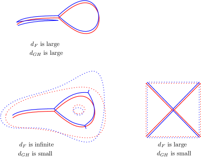
Figure 1. Comparison between Fréchet ($d_{F}$) and Gromov-Hausdorff ($d_{GH}$) stability. On the two examples below, the shapes are ($\lambda,\alpha$)-filtered medial axes of nearby sets (in dotted lines), and as asserted by Theorem 11.1, the Gromov-Hausdorff distance between them is small.

[Figures with pairs of spaces with the Fréchet and Gromov-Hausdorff distance]On the top one sees a figure with a zigzag in blue and one without in red. This makes both the Fréchet and Gromov-Hausdorff distance large. On the bottom left one sees two medial axis that are close, but not homeomorphic (due to some small Y-branching). In this case the Fréchet is infinite, while the Gromov-Hausdorff distance in very small. In the final panel one sees two medial axis that are perturbations of a cross (X) where in one case the crossing point is perturbed into a small horizontal line segment and in the other case in a small vertical line segment. The homeomorphism that maps the two perturbed crosses onto each other has to rotate the shape 90 degrees, so that the Fréchet distance is large. The Gromov-Hausdorff in the other hand is small.

Gromov-Hausdorff stability can be seen informally as a weakening of Frechet distance that ignores small scale features.

4. Motivation

4.1. Medial axis computation algorithms and models of computation

The medial axis is known to be unstable in theory (Attali et al., 2009), and, as a consequence, its computation is often problematic in practice. A typical illustration of this instability is when $K^{c}$ is an open disk in the plane: its medial axis is a point, but a $C^{\infty}$ perturbation, arbitrary small, in the $C^{0}$ sense of differential topology (Hirsch, 1976), of its boundary, may produce an arbitrary large perturbation (measured in the Hausdorff distance) of the resulting medial axis.

Computing the medial axis consists in, given as input some representation of the closed set $K$, to compute as output some representation of $\operatorname{{ax}}(K)$. Let us recall two possible computation models under which what it means to “compute” $K\mapsto\operatorname{{ax}}(K)$.

In computational geometry, the implicit computation model (sometimes called exact computation paradigm in order to distinguish it from the unrealistic “Real RAM” computation model) assumes that both input and output can be exactly represented by finite data in the computer. This implies that input and output have to belong to countable sets, such as, for example, integer, rational or algebraic numbers, or polynomials built on top of them. Given a set of rational or algebraic points, or given a polyhedron with rational or algebraic vertices coordinates, for example, we now that the medial axis is a finite algebraic complex and, as such, belongs to a countable set, therefore exactly presentable on a computer. These are situations where it makes sense to compute the medial axis in this exact computation model, even if it may be difficult.

Computable analysis, pioneered with the notion of computable real numbers introduced by Turing in his 1936 undecidability paper (Turing, 1937, 2004), is studied in the logic and theoretical computer science literature (Grzegorczyk, 1955; Lacombe, 1955a, b, c, d; Ko, 1991; Weihrauch, 2000; Brattka et al., 2008; Battenfeld, 2008), but its formalism is most often ignored in applications.

However, it is actually implicit in many practical computations involving real numbers and real functions, for example in numerical analysis, where a typical example would be the finite element method. In this context, one considers that input and output can belong to topological spaces with countable bases of neighbourhoods, typically metric spaces with dense countable subsets, called separable metric spaces, who, as a consequence, have at most the cardinality of real numbers. Examples of such metric spaces are:

• Real numbers with their natural topology (rational numbers are dense).

• Continuous functions on a compact set with the sup norm (polynomials with rational coefficients are dense, by the Stone-Weierstrass Theorem).

• $L^{p}$ (classes of) functions with their associated $L^{p}$ norms (rational step functions are dense).

• Compacts subsets of Euclidean spaces endowed with the Hausdorff distance (finite points sets in $\mathbb{Q}^{n}$ are dense).

In the context of these separable metric spaces, an algorithm, in this model of computation, takes as input a sequence belonging to the dense subset, so that each element of the sequence, belonging to a countable space, admits a finite representation. It then computes, for each element of the input sequence, an element of the output sequence in such a way that the output sequence converges to the image of the limit of the input sequence. This mere definition assumes that the (theoretical) output of the limit of the input sequence, is the limit of the sequence of (actual) outputs of items of the input sequence. This is the reason why, in the context of computable analysis, only continuous functions, that commute with limits, can be computable. For example, integer part function is computable, in this model, only at non-integer numbers. In decimal representation, if, after the dot, an infinite sequence of $9$s appears, the algorithm would read the input forever.

Recall that a continuous function $\omega:{\mathbb{R}_{\geq 0}\rightarrow\mathbb{R}_{\geq 0}}$, with $\omega(0)=0$, is a modulus of continuity of a map $f:X\rightarrow Y$ between metric spaces if for all $x_{1},x_{2}\in X$,

$$d_{Y}(f(x_{1}),f(x_{2})) \leq\omega(d_{X}(x_{1},x_{2})).$$

If one wishes to control some form of theoretical algorithmic efficiency in the context of computable analysis, a modulus of continuity of the operator, that associates to some uncertainty on the input an upper bound on the induced uncertainty on the output, needs to be estimated.

We do not need to enter here in the technicalities of computable analysis. Our contribution consists in stating some explicit modulus of continuity, which, on the theoretical side, would be a crucial ingredient in the proofs of computability and complexity in the context of computable analysis, but is also, on the application side, a way to guarantee some accuracy in practical computations. Indeed, practical implementations of the computation of the medial axis apply some kind of approximation during the computation process. In a practical situation, this approximation process is already inherent to the data collection process, as any physical numerical measure is meant at some, finite, accuracy. Second, the actual input of an algorithm is often the output of a preceding algorithm which cannot, reasonably, be assumed recursively to compute exact output from exact inputs: recursion on algebraic numbers representations are possible along a finite depth of computation only. When, along the process, some form of rounding, pixelization, small features collapses or filtering, is performed, being able to upper bound the impact on the output seems sensible, and in fact necessary for provably correct algorithms.

Since $K\mapsto\operatorname{{ax}}(K)$ is not continuous in general when the topology of both inputs and outputs are defined by the Hausdorff distance, we see two ways of stating a continuity, or stability, property, for the operator $K\mapsto\operatorname{{ax}}(K)$. One possibility is to consider a stronger topology on the input, a form of Fréchet, or ambient diffeomorphism based, $C^{k}$ distance, which would apply to smooth objects and representations.

Another possibility is to consider a weaker topology on the output, by considering filtered medial axes. In this model, the input sequence encodes $K$ in the form of approximations $\big{(}\tilde{K}_{i}\big{)}_{i\in\mathbb{N}}$ that converge to $K$ in Hausdorff distance. For the $\tilde{K}_{i}$ one would typically choose finite point sets or (geometric) simplicial complexes (meshes/triangulations). As $i$ would increase in one would not only add more points or simplices to $K_{i}$, but also make the coordinates of the points/vertices more precise by adding digits to their coordinates.

The output sequence encodes $\operatorname{{ax}}(K)$, in the form of progressive approximations of the map $(\lambda,\mu)\mapsto\operatorname{{ax}}_{\lambda}^{\alpha}(K)$, for decreasing values of $\lambda,\alpha$. These approximations (effectively) converge, where a basis of neighbourhoods (in the space of functions) of $(\lambda,\alpha)\mapsto\operatorname{{ax}}_{\lambda}^{\alpha}(K)$ is given by the sets of maps $(\lambda,\alpha)\mapsto f(\lambda,\alpha)$ satisfying $\lambda,\alpha>t\Rightarrow d_{\star}(f(\lambda,\alpha),\operatorname{{ax}}_{\lambda}^{\alpha}(K))<\epsilon$ for some $\epsilon,t>0$.

This approach does not require any smoothness assumption on $K$. The present paper focuses on this filtered approach, where the considered distance $d_{\star}$ between sets is either the Hausdorff distance, either the Gromov-Hausdorff distance on geodesic metric spaces.

Describing formally effective types and algorithms for the computation of the medial axis is beyond the scope of this paper. However, let us make some suggestions for further work in this direction. Probably the simplest model would consider the space of finite set of points with rational coordinates as inputs. These inputs together form a countable, and recursively enumerable set which is naturally equipped with the Hausdorff distance. The topological completion of the set of inputs gives all compact subsets of Euclidean space. The corresponding output space would consist of the filtered Voronoi Diagrams for which the coordinates of the Voronoi vertices are rational numbers. The Hölder modulii of continuity proven in this paper would allow to formally state the effectivity of the model.

The model could also be formalized in the context of Scott domains (Abramsky and Jung, 1994; Edalat and Heckmann, 1998), (Amadio and Curien, 1998, Chapter 1) and their associated information orders. In this context, our results answer the following question: If the only information we have about some compact set $K$ is its Hausdorff approximation $K^{\prime}$, what information can we infer about its medial axis $\operatorname{{ax}}(K)$?

4.2. Motivation from mathematics: the stability of the cut locus.

The medial axis is closely related to the cut locus. We recall

Definition 4.1.

Let $\mathcal{M}$ be a smooth (closed) Riemannian manifold and let $p\in\mathcal{M}$. For every $v\in T_{p}\mathcal{M}$, with $|v|=1$, we can consider the geodesic $\gamma_{v}(t)=\exp_{p}(tv)$ emanating from $p$ in the direction $v$. Let $\gamma_{v}(\tau)$ be the first point along $\gamma_{v}$ such that the geodesic $\{\gamma_{v}(t)\mid t\in[0,\pi]\}$ is no longer the unique minimizing geodesic to $p$. The cut locus of $p$ is the union of these points for all unit length $v$ in $T_{p}\mathcal{M}$.

The cut locus is therefore more general in the sense that it is defined for general Riemannian manifolds, while more restrictive in the sense that it only considers a single point.

The stability and structure of the singularities of the cut locus has been a studied intensely. Buchner (Buchner, 1977) derived the following result:

Theorem 4.2.

Let $G$ be the space of metrics on a smooth manifold, endowed with the Whitney topology. Each metric $g\in G$ and $p\in\mathcal{M}$ yield a cut locus $C_{p,g}$. The cut locus $C_{p,g}$ is called stable if there is a neighbourhood $W\subset G$ of $g$ such that for any $g^{\prime}\in W$ there exists a diffeomorphism $\Phi:\mathcal{M}\to\mathcal{M}$ such that $\Phi(C_{p,g^{\prime}})=C_{p,g}$. If the dimension of $\mathcal{M}$ is low ($\leq 6$) then $C_{p,g}$ is stable for an open and dense subset of $G$.

Wall (Wall, 1977) extended this result to arbitrary dimensions at the cost of weakening the diffeomorphism to a homeomorphism. The structure of the singularities of the cut locus were also described by Buchner in (Buchner, 1978). A similar description for the singularities of medial axis of a smooth manifold can be found in (Yomdin, 1981), see also (Mather, 1983), as well as (van Manen, 2007).

This paper follows the tradition of these investigations of the stability of cut locus and the medial axis. However, there are also some significant differences. First and foremost we take a metric viewpoint instead of analytical. This viewpoint does not require us to make a distinction between low dimensional and high dimensional spaces. We made the constants explicit in view of the applications in computer science, in particular computational geometry and topology, shape recognition, shape segmentation, and manifold learning.

The authors are currently working on the stability of the cut locus and medial axis of smooth sets, using the tools which we develop in this paper.

5. Overview of the stability of the $\lambda$-medial axis

Under mild conditions, the $\lambda$-medial axis enjoys some nice stability properties, assuming that $K^{c}$ is bounded. Informally:

1. When $\chi_{K}$ does not vanish on $(0,\lambda]$, the $\lambda$-medial axis preserves the homotopy type of the complement $K^{c}$ of $K$ (Chazal and Lieutier, 2005a, Theorem 2),

2. Taking the Hausdorff distance on the input $K$ and the one sided Hausdorff distance on the output $\operatorname{{ax}}_{\lambda}(K)$ we get a kind of modulus of continuity. If $d_{h}(K,K^{\prime})$ is small, the points in $\operatorname{{ax}}_{\lambda}(K)$ are “near”, in a quantified way, $\operatorname{{ax}}_{\lambda^{\prime}}(K^{\prime})$, for some $\lambda^{\prime}<\lambda$ close to $\lambda$ (Chazal and Lieutier, 2005a, Theorem 3).

3. For “regular values of $\lambda$” the map $K\mapsto\operatorname{{ax}}_{\lambda}(K)$ is continuous for the Hausfdorff distance (Chazal and Lieutier, 2005a, Theorem 5). However, the modulus of continuity can be arbitrarily large in general.

Property 1 gives some stability on the homotopy type with respect to Hausdorff perturbation of $K$, since, under similar conditions on the critical function of $K$, when $d_{h}(K,K^{\prime})$ is small, the offsets of $K^{\prime}$ may share the homotopy type of $K$ (Chazal and Lieutier, 2005b; Chazal et al., 2009). Properties 2 and 3 give precise, quantified, stability results, much stronger than the mere half-continuity of the medial axis itself, see e.g. (Attali et al., 2009).

6. Contributions: the improved stability of the $(\lambda,\alpha)$-medial axis

Before entering into the formal proofs, let us give some intuition about the $(\lambda,\alpha)$-medial axis stability.

This improved stability can be illustrated in the case of a finite set $K$. Figure 2 illustrates the $(\lambda,\alpha)$-medial axis in the simplest non-trivial case, where $K$ consists of two points in the plane. In this case the $\lambda$-medial axis would be empty as long as $\lambda$ is strictly greater than the half distance between the two points and it would become the whole bisector line as soon as $\lambda$ is smaller or equal to this value.

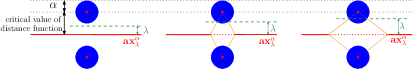
Figure 2. Comparison between $\lambda$-medial axis and $(\lambda$,$\alpha)$-medial axis evolutions for increasing $\lambda$, in the particular case where $K$ consists of two points in the plane. The $\lambda$-medial axis would be either the whole bisector line of the two points, for $\lambda$ smaller or equal to half the distance between the points, either the empty set for larger value of $\lambda$. By contrast, the evolution, for increasing $\lambda$, of the $(\lambda,\alpha)$-medial axis, which is also the $\lambda$-medial axis of the union of two disks of radius $\alpha$, evolves continuously, in Hausdorff distance, as $\lambda$ increases.

The $\lambda$-medial axis and $(\lambda$,$\alpha)$-medial axis of two points in the plane.

By contrast, the $(\lambda,\alpha)$-medial axis, for a fixed value of $\alpha>0$, here the radius of the two disks of the $\alpha$-offset of $K$, is Hausdorff continuous with respect to $\lambda$. Indeed, as $\lambda$ increases, when $\alpha+\lambda$ equals the half distance between the two points, $\operatorname{{ax}}_{\lambda}^{\alpha}(K)$, which until then is the whole bisector line, starts to be disconnected, creating a hole. But, since the hole grows continuously, its birth is not a discontinuity for the Hausdorff distance. However, in the neighborhood of this event, the hole size grows quadratically with $\lambda$: This does not contradict the claim that the map $\lambda\mapsto\operatorname{{ax}}_{\lambda}^{\alpha}(K)$ is Lipschitz, as the precise conditions of the claim require us to avoid situations where $\alpha+\lambda$ is a zero of $\chi_{K}$.

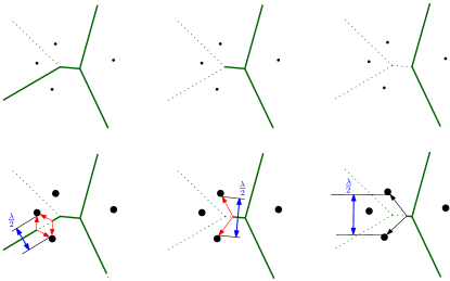
Figure 3. Comparison between $\lambda$-medial axis and $(\lambda$,$\alpha)$-medial axis evolutions for increasing $\lambda$, in the particular case where $K$ is a finite subset of the plane. In this case both filtered medial axes are subsets of the union of the edges of the Voronoi diagram. On the second row, the points have been replaced by disks of radius $\alpha$, offset of the points. The evolution of the $(\lambda$,$\alpha)$-medial axis is Hausdorff continuous whenever $\alpha+\lambda$ is not a critical value of the distance function. On the other hand, as seen on first row, the $\lambda$-medial axis contains precisely the whole Voronoi edges or vertices whose dual simplex lies in a ball of radius $\lambda$. The $\lambda$-medial axis is therefore Hausdorff discontinuous for each value of $\lambda$ which is the radius of the smallest ball enclosing some Delaunay simplex.

[The $\lambda$-medial axis and $(\lambda$,$\alpha)$-medial axis of four points in the plane.]The $\lambda$-medial axis and $(\lambda$,$\alpha)$-medial axis of four points in general position in the plane (for various values of $\lambda$). The points are arranged as follows: Three on the left and one on the right. The three points on the left form an obtuse triangle arranged in such a way that its circumcentre, one point on the left and the point on the right lie very close to a horizontal line. The two other points on the left lie on either side of the horizontal line and nearly above/below each other.

Figure 3 shows a situation where $K$ is made of four points in the plane. The $\lambda$-medial axis is made of these edges and vertices whose dual Delaunay simplex has smallest enclosing radius greater or equal to $\lambda$. As a function of $\lambda$, it is therefore Hausdorff distance discontinuous for each value of $\lambda$ that is equal to a such radius.

In contrast, the $(\lambda,\alpha)$-medial axis, as a function of $\lambda$ for fixed $\alpha>0$, can be Hausdorff discontinuous only when $\alpha+\lambda$ is a zero of the critical function $\chi_{K}$. We have depicted such a transition in Figure 4: Here we increase $\lambda$ further until $\alpha+\lambda=\rho$, where $\rho$ is the circumradius of the unique acute triangle in the Delaunay diagram, and therefore the unique value of the distance to $K$ corresponding to a local maximum. Until $\alpha+\lambda=\rho$ the $(\lambda,\alpha)$-medial axis would contain the Voronoi vertex dual to this acute triangle (for $\alpha+\lambda=\rho$ the Voronoi vertex would be an isolated point). Since this points would disappear from the $(\lambda,\alpha)$-medial axis for $\alpha+\lambda>\rho$, it results a Hausdorff distance discontinuity of $\lambda\mapsto\operatorname{{ax}}_{\lambda}^{\alpha}(K)$.

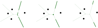
Figure 4. Further evolution of the ($\lambda$,$\alpha$)-medial axis, after the steps of the bottom row of figure 3. For some small interval of values of $\lambda$, the Voronoi vertex is an isolated point on $\operatorname{{ax}}_{\lambda}^{\alpha}(K)$, as illustrated on the middle, When $\alpha+\lambda$ equals the Delaunay triangle circumradius, this points disappears from $\operatorname{{ax}}_{\lambda}^{\alpha}(K)$, which corresponds to a discontinuity of $\lambda\rightarrow\operatorname{{ax}}_{\lambda}^{\alpha}(K)$ for the Hausdorff distance.

The same configuration of points in the plane as in the previous figure (Figure 3).

In general, Hausdorff distance discontinuities of $\lambda\mapsto\operatorname{{ax}}_{\lambda}(K)$ may appear anywhere, at some “non regular values”, as mentioned in item 3 of Section 5 and illustrated on top row of Figure 3 (where $\lambda$ is a zero of $\chi_{K}$) and in Figure 9 (where $\lambda$ is not a zero of $\chi_{K}$). By contrast, the map $\lambda\mapsto\operatorname{{ax}}_{\lambda}^{\alpha}(K)$, for $\alpha>0$, is continuous (locally Lipschitz) when $\chi_{K}(\alpha+\lambda)$ does not vanish, in other words the interval on which the homotopy type of $\operatorname{{ax}}_{\lambda}^{\alpha}(K)$ remains stable.

6.1. The case of a set $K\subset\mathbb{R}^{n}$ with positive $\mu$-reach and its Hausdorff approximation $K^{\prime}$

In Part II: The technical statements and proofs we consider the general situation of sets whose $\alpha$-offsets have positive $\mu$-reach. In particular, Lemma 10.7 and Theorem 11.1 use a symmetrical formulations on the pair of sets $K$ and $K^{\prime}$ in order to state a modulus of continuity for the map $K\mapsto\operatorname{{ax}}_{\lambda}^{\alpha}(K)$, where the metric on $K$ is the Hausdorff distance and the metric on the medial axis can be either the Hausdorff distance or the Gromov-Hausdorff distance.

In this section we consider the simpler setting, where we don’t need to offset for $K$ to achieve positive $\mu$ reach, that is $r_{\mu}(K)>0$ and we are given a set $K^{\prime}$ that is close to $K$ in terms of the Hausdorff distance. This allows a concise formal expression of our main results in a simpler setting, while illustrating a typical application.

Overall this section, we make the following assumption:

Assumption 6.1 (Assumption for Section 6.1).

We assume $K,K^{\prime}$ to be closed sets such that, for some $\epsilon>0$, $d_{H}(K^{\prime},K)<\epsilon$, $r_{\mu}(K)>0$ and, the complements $K^{c}$ and $K^{\prime c}$ to be bounded: denoting $\operatorname{\mathbb{B}}(0,R)\subset\mathbb{R}^{n}$ the ball of radius $R>0$, one has $K\cup\operatorname{\mathbb{B}}(0,R)=K^{\prime}\cup\operatorname{\mathbb{B}}(0,R)=\mathbb{R}^{n}$. We assume moreover $0<\alpha<\alpha_{\max}$ and $0<\lambda<\lambda_{\max}$, for $\alpha_{\max}+\lambda_{\max}<r_{\mu}(K)/2$ and we denote $\tilde{\mu}=\min(\mu,\sqrt{3}/2)$.

In particular, assuming $\alpha_{\max}+\lambda_{\max}<r_{\mu}(K)/2$ allows a simple expression for $\tilde{\mu}$.

6.1.1. Hausdorff stability

As a consequence of Lemma 9.4 and Lemma 9.5 we have that:

Proposition 6.2.

For any $\lambda_{\min}>0$, the map $\lambda\mapsto\operatorname{{ax}}_{\lambda}^{\alpha}(K)$ is $\left(\frac{R^{2}}{\alpha\lambda_{\min}\tilde{\mu}^{2}}\right)$-Lipschitz in the interval $[\lambda_{\min},\lambda_{\max}]$ for Hausdorff distance.

Similarly, for $\alpha_{\min}>0$, the map $\alpha\mapsto\operatorname{{ax}}_{\lambda}^{\alpha}(K)$ is $\left(\frac{R^{2}}{\alpha_{\min}\lambda\tilde{\mu}^{2}}\right)$-Lipschitz in the interval $[\alpha_{\min},\alpha_{\max}]$ for Hausdorff distance.

We will now combine this with a result from (Chazal et al., 2009, Theorem 3.4). Let $\mu^{\prime}<\mu$ and $\alpha>0$. By definition of $r_{\mu}(K)$, the critical function of $K$ is above $\mu$ on the interval $(0,r_{\mu}(K))$. Theorem 3.4 of (Chazal et al., 2009) now says that if $K^{\prime}$ is sufficiently close to $K$ in Hausdorff distance, then the critical function of $K^{\prime}$ will also be above $\mu^{\prime}$ on the interval $(\alpha,r_{\mu}(K)-\alpha)$, see Figure 7. In other words, there is $\epsilon>0$ such that:

(3) $$d_{H}(K^{\prime},K)<\epsilon\Rightarrow r_{\mu^{\prime}}^{\alpha}(K^{\prime})>r_{\mu}(K)-\alpha.$$

Then, Lemma 10.7 gives us that:

Proposition 6.3.

Denoting $\tilde{\mu}^{\prime}=\min(\mu^{\prime},\sqrt{3}/2)$, there is $\epsilon_{\max}>0$ depending only on $K$, such that, for, $\epsilon<\epsilon_{\max}$, one has:

(4) $$d_{H}\left(\operatorname{{ax}}_{\lambda}^{\alpha}(K^{\prime}),\operatorname{{ax}}_{\lambda}^{\alpha}(K)\right)<\frac{22}{3}\frac{R^{2}}{\alpha^{\frac{1}{2}}\tilde{\mu}^{\prime\frac{3}{2}}\lambda}\>\epsilon^{\frac{1}{2}}.$$

Note that, thanks to (Chazal et al., 2009), under the conditions of the proposition, that is for sufficiently small $\epsilon$, $\operatorname{{ax}}_{\lambda}^{\alpha}(K^{\prime})$, $\operatorname{{ax}}(K)$ and $K^{c}$ have same homotopy type (Theorem 9.7 below).

6.1.2. Gromov-Hausdorff stability

Lemma 9.11 and Theorem 9.12 give an explicit upper bound in the geodesic diameter of $\operatorname{{ax}}_{\lambda}^{\alpha}(K)$, assuming $K^{c}$ to be connected, as:

(5) $${\operatorname{GeoDiameter}}(\operatorname{{ax}}_{\lambda}^{\alpha}(K))\leq 2\frac{R}{\tilde{\mu}^{2}}+2\alpha\left(\left(\frac{4R}{\alpha}\right)^{n}+1+\frac{2}{\mu}\right)e^{\frac{1}{\mu}+\frac{R}{\alpha\tilde{\mu}^{2}}}$$

Thanks to (3), a similar bound holds for ${\operatorname{GeoDiameter}}(\operatorname{{ax}}_{\lambda}^{\alpha}(K^{\prime}))$, for sufficiently small $\epsilon$.

This bound is exponential in $\frac{2R}{\alpha\tilde{\mu}^{2}}$ and therefore increases quickly as $\alpha\rightarrow 0$. We do not know if this bound is close to be tight.

Lemmas 9.14 and 9.15 give:

Proposition 6.4.

For any $\lambda_{\min}>0$, the map $\lambda\mapsto\operatorname{{ax}}_{\lambda}^{\alpha}(K)$ is $\left(\frac{R^{2}(2\alpha_{\min}\lambda_{\min}+D}{\alpha_{\min}^{2}\tilde{\mu}^{2}}\right)$-Lipschitz in the interval $[\lambda_{\min},\lambda_{\max}]$ for Gromov-Hausdorff distance, where

$$D=\max_{\lambda\in[\lambda_{\min},\lambda_{\max}]}{\operatorname{GeoDiameter}}(\operatorname{{ax}}_{\lambda}^{\alpha}(K)).$$

Similarly, for $\alpha_{\min}>0$, the map $\alpha\mapsto\operatorname{{ax}}_{\lambda}^{\alpha}(K)$ is $\left(\frac{R(2\alpha_{\min}+D}{\alpha_{\min}^{2}\tilde{\mu}^{2}}\right)$-Lipschitz in the interval $[\alpha_{\min},\alpha_{\max}]$ for Gromov-Hausdorff distance, where $D=\max_{\lambda\in[\alpha_{\min},\alpha_{\max}]}{\operatorname{GeoDiameter}}(\operatorname{{ax}}_{\lambda}^{\alpha}(K))$.

Note that the geodesic diameter enters as a factor in the Lipschitz constant. This is due to the fact that the Gromov-Hausdorff distance is defined as a global upper bound on differences of lengths, while, here, the metrics differ mainly by a multiplicative factor. In a sense, the metric discrepancy would be more tightly bounded by a mix of additive and multiplicative bounds, where Gromov-Hausdorff distances consider additive discrepancy only. Replacing $D$ by its universal upper bound (5) is likely, in general, to give an overestimated Lipschitz constant with respect to the one using the actual diameter $D=\max_{\lambda\in[\alpha_{\min},\alpha_{\max}]}{\operatorname{GeoDiameter}}(\operatorname{{ax}}_{\lambda}^{\alpha}(K))$.

Also, Theorem 11.1 gives us:

Proposition 6.5.

Denoting $\tilde{\mu}^{\prime}=\min(\mu^{\prime},\sqrt{3}/2)$, there is $\epsilon_{\max}>0$ depending only on $K$, such that, for, $\epsilon<\epsilon_{\max}$, one has:

(6) $$d_{GH}\left(\operatorname{{ax}}_{\lambda}^{\alpha}(K^{\prime}),\operatorname{{ax}}_{\lambda}^{\alpha}(K)\right)<2\left(\frac{22}{3}\right)^{\frac{3}{2}}\frac{R^{3}(2\alpha_{\min}+D)}{\alpha_{\min}^{\frac{7}{4}}\tilde{\mu}^{\prime\frac{9}{4}}\lambda^{\frac{3}{2}}}\>\epsilon^{\frac{1}{4}},$$

where $D=\max({\operatorname{GeoDiameter}}(\operatorname{{ax}}_{\lambda}^{\alpha}(K)),{\operatorname{GeoDiameter}}(\operatorname{{ax}}_{\lambda}^{\alpha}(K^{\prime})))$.

Again, taking for $D$ the upper bound (5) allows a uniform bound which is enough in theory.

For a more practical bound on $d_{GH}\left(\operatorname{{ax}}_{\lambda}^{\alpha}(K^{\prime}),\operatorname{{ax}}_{\lambda}^{\alpha}(K)\right)$ it would be easier to calculate a bound on the geodesic diameter of $\operatorname{{ax}}_{\lambda}^{\alpha}(K^{\prime})$. For example, if $K^{\prime}$ is finite (in fact the union of the complement of $\operatorname{\mathbb{B}}^{\circ}(0,R)$ with a finite set) one could determine a bound on the geodesic diameter of the subset of the $(n-1)$-skeleton of part of the Voronoi diagram corresponding to $\operatorname{{ax}}_{\lambda}^{\alpha}(K^{\prime})$.

6.2. Method

All proofs in the paper are based on the flow of the (generalized) gradient of the distance function from a point $x$ to $K$, see Section 8.2 for a formal definition. The flow has been used before, among others to establish the following results:

• The medial axis has the same homotopy type as the set (Lieutier, 2004).

• The topologically guaranteed reconstruction for non-smooth sets (Chazal et al., 2009).

The flow also plays a central role in the work on the $\lambda$-medial axis (Chazal and Lieutier, 2005a). These tools were developed for non-smooth objects, and rely on the weak regularity properties based on the $\mu$-reach and the critical function (Section 8.2). Our stability results rely on the stability of the flow and its gradient under Hausdorff perturbation of $K$, and by quantifying how quickly we enter the $(\lambda,\alpha)$-medial axis following the flow of the gradient, assuming that we start not too far from the $(\lambda,\alpha)$-medial axis.

7. Future work

Beyond the stability properties presented in this paper, several questions remain open. We do not know if our moduli of continuity are optimal, or if other filtrations could offer better Hölder exponents for the stability. More precisely, because the dependence of the ($\lambda$,$\alpha$)-medial axis on $\lambda$ and $\alpha$ is Lipschitz, it is only the Lipschitz constant that can be improved. This contrasts with the Hölder exponents for the map $K\mapsto\operatorname{{ax}}_{\lambda}^{\alpha}$, namely $\frac{1}{2}$ for the Hausdorff distance and $\frac{1}{4}$ the Gromov-Hausdorff distance, which may not be optimal.

Our stability property expressed in term of Gromov-Hausdorff distance hides a stronger statement. Indeed the Gromov-Hausdorff distance applies to two independent metric spaces, while our two metric spaces are also subset of a same Euclidean space. While this has not been made explicit in the statement of Theorem 11.1, when $d_{H}(K,K^{\prime})<\epsilon$, (82) gives a $\mathcal{O}(\epsilon^{\frac{1}{2}})$ bound on the ambient Euclidean distance between points pairs in relation that upper bounds the $\mathcal{O}(\epsilon^{\frac{1}{4}})$ Gromov-Hausdorff distance. For example, in Figure 1 on the right, a simple rotation could define a relation giving a zero Gromov-Hausdorff distance (an isometry), while in fact our construction defines another relation for which points in relation are much closer in ambient space. In order to fully express our stability properties induced by the flow, we should introduce in a future work a sharpening of the Gromov-Hausdorff distance, where the relation realizes not only a small geodesic metric distortion, but also a small ambient displacement.

Part II: The technical statements and proofs

8. Definitions and previous work

In this section, we recall some definitions and results, mainly introduced in (Lieutier, 2004; Chazal and Lieutier, 2005a; Chazal et al., 2009), in order to make the paper self-contained.

Throughout the paper, $K$ will be a closed subset of $\mathbb{R}^{n}$, whose complement $K^{c}$ is bounded and connected.The fact that $K^{c}$ is connected is essential for the medial axis to be patch connected and thus is needed for a bound on the geodesic diameter. The geodesic diameter in turn is needed for the bound on the Gromov-Hausdorff distance (our bound is proportional to the geodesic diameter). We stress that the connectedness assumption is not required for our results on the Hausdorff distance.

8.1. Homotopy equivalence and weak deformation retraction

A homotopy equivalence between topological spaces $X$ and $Y$ where $Y\subset X$ and the map from $Y$ to $X$ is the inclusion map, is called weak deformation retract, more formally:

Definition 8.1 (weak deformation retract).

If $Y\subset X$ and there exists a continuous map $H:[0,1]\times X\rightarrow X$ such that:

• $\forall x\in X,\>H(0,x)=x$,

• $\forall x\in X,\>H(1,x)\in Y$,

• $\forall y\in Y,\forall t\in[0,1],\>H(t,y)\in Y$,

then we say that $H$ is a weak deformation retract of $X$ on $Y$. In particular $X$ and $Y$ have same homotopy type.

8.2. The medial axis and associated flow

We define the following functions on $\mathbb{R}^{n}$ associated to $K$:

(7) $$x\mapsto R_{K}(x) \underset{\text{def.}}{=}\>d(x,K)=\min_{y\in K}d(x,y)$$

(8) $$x\mapsto\Theta_{K}(x) \underset{\text{def.}}{=}\>\left\{y\in K\mid d(x,y)=R_{K}(x)\right\}.$$

For a bounded set $S$ we denote the center of the smallest ball enclosing $S$ by $\operatorname{center}(S)$, we write $\operatorname{radius}(S)$ for the radius of this ball.

We further define,

(9) $$\operatorname{\mathcal{F}}_{K}(x)\underset{\text{def.}}{=}\>\operatorname{radius}(\Theta_{K}(x))$$

and for $x\notin K$:

(10) $$\nabla_{K}(x)\underset{\text{def.}}{=}\>\frac{x-\operatorname{center}(\Theta_{K}(x))}{R_{K}(x)}$$

The medial axis $\operatorname{{ax}}(K)$ of $K$ is defined as:

(11) $$\operatorname{{ax}}(K)\underset{\text{def.}}{=}\>\{x\in\mathbb{R}^{n}\mid\operatorname{\mathcal{F}}_{K}(x)>0\}=\{x\in\mathbb{R}^{n}\mid\sharp\left(\Theta_{K}(x)\right)\geq 2\}$$

where $\sharp X$ denotes the cardinality of the set $X$.

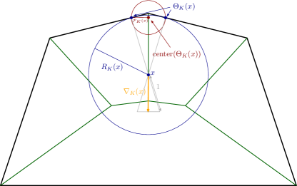
Figure 5. Pictorial overview of the definitions and notation. The set $K$ is indicated in black and the medial axis in green.

A pentagon and its medial axis with the notation indicated.

When $x\in K$, one has $\Theta_{K}(x)=\{x\}$ and $\operatorname{\mathcal{F}}_{K}(x)=0$. It follows that $\operatorname{{ax}}(K)\subset K^{c}$.

When $x\notin K\cup\operatorname{{ax}}(K)$, $\nabla_{K}(x)$ coincides with the gradient of the Lipschitz function $x\mapsto R_{K}(x)$.

For any $x\in K^{c}$, including when $x\in\operatorname{{ax}}(K)$, $\nabla_{K}(x)$ could have been equivalently defined as the projection of $0$ on the Clarke gradient, see (Clarke, 1990), of $x\mapsto R_{K}(x)$. However the definition (10) is more convenient in our context and does not require the formal introduction of Clarke gradient, which is technical. For this reason, we call $\nabla_{K}(x)$ the generalized gradient of $x\mapsto R_{K}(x)$. Thanks to the definition of $\nabla_{K}(x)$, and Pythagoras, see that for $x\notin K$ one has:

(12) $$\forall x\in K^{c},\quad\left\|\nabla_{K}(x)\right\|^{2}=1-\left(\frac{\operatorname{\mathcal{F}}_{K}(x)}{R_{K}(x)}\right)^{2}.$$

In (Lieutier, 2004) we have seen that there exists a locally Lipschitz, and therefore continuous, flow $\Phi_{K}:{\mathbb{R}_{\geq 0}}\times K^{c}\rightarrow K^{c}$ such that:

$$\forall x \in K^{c}, \Phi_{K}(0,x) =x$$

(13) $$\forall x \in K^{c}\>,\forall t\geq 0, \frac{d}{dt^{+}}\Phi_{K}(t,x) =\nabla_{K}\left(\Phi_{K}(t,x)\right)$$

(14) $$\forall x \in K^{c},\>\forall t_{1},t_{2}\geq 0, \Phi_{K}\left(t_{1},\Phi_{K}(t_{2},\,x)\right) =\Phi_{K}(t_{1}+t_{2},\,x).$$

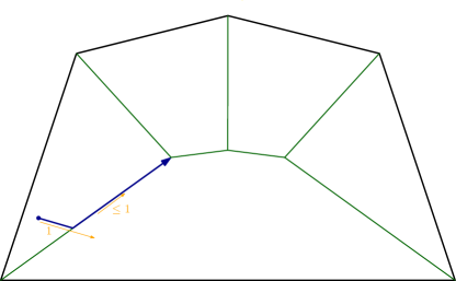
Figure 6. The blue path follows the flow. The orange vectors indicate the vectors ($\nabla_{K}(x)$) whose flow $\Phi_{K}$ follows. They have been shifted slightly for visibility and lengths have been indicated.

The same pentagon and medial axis as before with the flow of $\nabla_{K}(x)$.

It was established in (Lieutier, 2004) that $\operatorname{{ax}}(K)$ has same homotopy type as $K^{c}$. This result is based on the fact that the flow $\Phi_{K}$ realizes the homotopy equivalence $K^{c}\rightarrow\operatorname{{ax}}(K)$ for a finite $t$ (see Definition 8.1). In the particular case when $K$ is a finite set, the flow $\Phi_{K}$ is equivalent to the flow that induces the flow complex (Giesen and John, 2008) of $K$.

We further recall the following:

Lemma 8.2 (Lemma 4.16 of (Lieutier, 2004)).

(15) $$\forall t \geq 0,\forall x\in K^{c}, \frac{d}{dt^{+}}R_{K}(\Phi_{K}(t,x)) =\left\|\nabla_{K}\left(\Phi_{K}(t,x)\right)\right\|^{2}.$$

Lemma 8.3 (Corollary 4.7 of (Lieutier, 2004)).

The map $\operatorname{\mathcal{F}}_{K}$ is upper semi-continuous.

Lemma 8.4 (Lemma 4.17 of (Lieutier, 2004)).

The map $t\mapsto\operatorname{\mathcal{F}}_{K}(\Phi_{K}(t,x))$ is non-decreasing (i.e. increasing but not necessarily strictly increasing) and therefore, by Lemma 8.3 right-continuous.

Lemma 4.13 of (Lieutier, 2004) immediately yields:

Corollary 8.5.

(16) $$R_{K}(x_{1}),R_{K}(x_{2})\geq\alpha\Rightarrow\|\Phi_{K}(t,x_{2})-\Phi_{K}(t,x_{1})\|\leq\|x_{2}-x_{1}\|\,e^{\frac{t}{\alpha}}.$$

8.3. Critical function, $\mu$-reach and Weak Feature Size

As we have seen in Section 2, the critical function $\chi_{K}:(0,\infty)\to[0,1]$, is defined as

(1) $$\chi_{K}(t)\underset{\text{def.}}{=}\>\inf_{R_{K}(x)=t}\sqrt{1-\left(\frac{\operatorname{\mathcal{F}}_{K}(x)}{R_{K}(x)}\right)^{2}}.$$

In this setting we say that the infimum over the empty set yields $1$.We’ll now discuss the intuition behind this function. The critical function provides us in a certain sense with some lower bound on the norm of the vector field $\nabla_{K}(x)$ whose flow ($\Phi_{K}$) we follow. Figure 7 illustrates the critical function when $K$ is a (hollow) square in $\mathbb{R}^{3}$. The medial axis of the square is an infinite prism, which is the product of the squares’s diagonals and the line orthogonal to the square supporting plane. The infimum in (1) is first attained along the square diagonals, where $\chi_{K}(t)=1/\sqrt{2}$ since there $\operatorname{\mathcal{F}}_{K}(x)=\frac{R_{K}(x)}{\sqrt{2}}$. Then when the offset reaches the square center we get $\operatorname{\mathcal{F}}_{K}(x)=R_{K}(x)$ and therefore $\chi_{K}(t)=0$. The topology of the offset then changes and, after this critical value, the $\inf$ is then reached on the line through the square center and orthogonal to the square supporting plane.

The critical function enjoys some stability properties with respect to Hausdorff distance perturbation (Chazal et al., 2009, Theorem 4.2), illustrated in Figure 7. If two sets $K$ and $K^{\prime}$ are close enough in Hausdorff distance, their critical functions $t\mapsto\chi_{K}(t)$ and $t\mapsto\chi_{K^{\prime}}(t)$ are close to each other, for $t$ large enough.

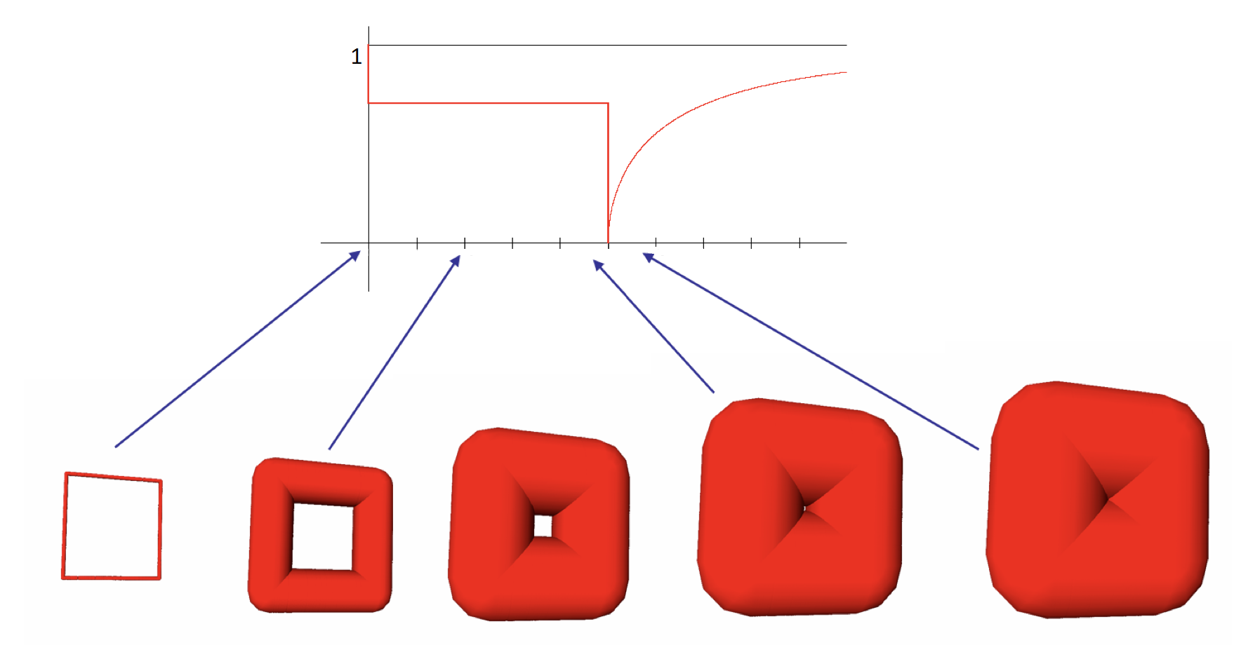
Figure 7. (Adapted from (Boissonnat et al., 2018))). On the top, the critical function $\chi_{K}$ of a square $K$ in $\mathbb{R}^{3}$ together with the corresponding level sets $R_{K}^{-1}(t)$ of the distance to $K$, on which the $\inf$ is taken in equation (1). The topology of offsets changes only when $\chi_{K}(t)=0$, that is when $t=t_{crit.}$ which is the half of the square side. For $t\in(0,t_{crit.})$, $\chi_{K}(t)=1/\sqrt{2}$ since, for $0<t<t_{crit.}$, the $\inf$ in (1) is For $t\in(0,t_{crit.})$ we have that $\chi_{K}(t)=1/\sqrt{2}$. This can be seen as follows: For $0<t<t_{crit.}$ the $\inf$ in (1) is attained on the intersection of $R_{K}^{-1}(t)$, the supporting plane of the square, and the medial axis. This intersection equals the diagonals of the square. It follows immediately from Pythagoras that $\operatorname{\mathcal{F}}_{K}(x)=\frac{R_{K}(x)}{\sqrt{2}}$. This value is indeed strictly smaller than $1$ as the reach of the square is $0$.
At the bottom, the critical function of a set $K^{\prime}$ (here a finite set), close, in Hausdorff distance, to $K$. For large enough offset $t$, $\chi_{K^{\prime}}$ is close to $\chi_{K}$. In particular, if $d_{H}(K^{\prime},K)$ is small enough with respect to $t_{crit.}$, Theorem (Chazal et al., 2009, Theorem 4.2) provides a lower bound on the critical function of $K^{\prime}$, which is then guaranteed to not vanish on some interval subset of $(0,t_{crit.})$.

The offset of a square (not filled in) and the critical function $\chi_{K}$.

The critical function has been introduced in Section 2 and illustrated in Figure 7. In (Chazal et al., 2009) the critical function $\chi_{K}:(0,\infty)\rightarrow[0,1]$ was defined for a compact set $K$. We adapt it to a closed set $K$ with bounded complement.

On a closed set $K$ with bounded complement the function $R_{K}$ attains a maximum:

(17) $$R_{\max}(K)\underset{\text{def.}}{=}\>\sup_{{x\in K^{c}}} R_{K}(x)=\max_{x\in K^{c}} R_{K}(x).$$

The critical function of $K$ is the function $\chi_{K}:(0,R_{\max}(K)]\rightarrow[0,1]$ defined as:

$$\chi_{K}(t)\underset{\text{def.}}{=}\>\inf_{R_{K}(x)=t}\|\nabla_{K}(x)\|.$$

As a consequence of (15), one has $\chi_{K}(R_{\max})=0$. For $\mu\in(0,1]$, the $\mu$-reach of $K$, denoted $r_{\mu}(K)$ is defined as:

$$r_{\mu}(K) \underset{\text{def.}}{=}\>\inf\{t\mid\chi_{K}(t)<\mu\}$$

$$=\,\sup\left\{r\mid R_{K}(x)<r\Rightarrow\|\nabla_{K}(x)\|\geq\mu\right\}.$$

For $\mu=1$, $r_{1}(K)$ is also known as the reach of $K$. The Weak Feature Size of $K$, denoted $\operatorname{wfs}(K)$ is defined as the first critical value of the distance function, that is the first value at which $\chi_{K}$ vanishes

(18) $$\operatorname{wfs}(K)\underset{\text{def.}}{=}\>\inf\{t\mid\chi_{K}(t)=0\}.$$

Since $x\mapsto\operatorname{\mathcal{F}}_{K}(x)$ is upper semi-continuous, see Corollary 4.7 of (Lieutier, 2004), $\chi_{K}$ is lower semi-continuous. The lower semi-continuity of $\chi_{K}$ has a number of consequences:

• If $0<\operatorname{wfs}(K)$, then we have $\chi_{K}(\operatorname{wfs}(K))=0$, so that

  $$\operatorname{wfs}(K)>0\Rightarrow\operatorname{wfs}(K)=\min\{t\mid\chi_{K}(t)=0\}.$$

  This follows by combining the lower semi-continuity with the definition of the weak feature size (18).

• By definition of $r_{\mu}(K)$ (and lower semi-continuity of $\chi_{K}$) we have that, for any $\mu>0$, $r_{\mu}(K)<\operatorname{wfs}(K)$.

• If $0<\sup\{r_{\mu}(K)\mid\mu>0\}<\infty$, then $\chi_{K}(\sup\{r_{\mu}(K)\mid\mu>0\})=0$. Because $\operatorname{wfs}(K)>0\Rightarrow\sup\{r_{\mu}(K)\mid\mu>0\}>0$, it follows that:

  (19) $$\operatorname{wfs}(K)>0\Rightarrow\operatorname{wfs}(K)=\sup\{r_{\mu}(K)\mid\mu>0\}.$$

8.4. Gromov-Hausdorff distance

For $\alpha\geq 0$, the $\alpha$-offset of $K$ denoted $K^{\oplus\alpha}$ is the set of points lying at distance at most $\alpha$ from $K$:

(20) $$K^{\oplus\alpha}\underset{\text{def.}}{=}\>\{x\in\mathbb{R}^{n}\mid d(x,K)\geq\alpha\},$$

where $d(x,K)\underset{\text{def.}}{=}\>\inf_{y\in K}d(x,y)=\min_{y\in K}d(x,y)$. Alternatively, $K^{\oplus\alpha}$ can be defined as the Minkowski sum of $K$ with a ball of radius $\alpha$ centered at $0$, which motivates the $\oplus$ notation.

The Hausdorff distance between two compact subsets $A,B$ of the Euclidean space is defined as ((Bridson and Haefliger, 2013, Section 5.30)):

Definition 8.6 (Hausdorff distance).

The Hausdorff distance between closed sets $A$ and $B$ is defined as

(21) $$d_{H}(A,B)=\inf\left\{\varepsilon,\>A\subset B^{\oplus\varepsilon}\>\mathrm{and}\>B\subset A^{\oplus\varepsilon}\right\}.$$

One trivially has,

(22) $$A\subset B\quad\mathrm{and}\quad B\subset A^{\oplus\varepsilon}\quad\Rightarrow\quad d_{H}(A,B)\leq\varepsilon.$$

We now define the Gromov-Hausdorff distance between two metric spaces $X_{1}$ and $X_{2}$. We follow (Bridson and Haefliger, 2013, Section 5.33), with minor modifications in the formulation for compatibility.

Definition 8.7 (Gromov-Hausdorff distance).

An $\varepsilon$-relation between two metric spaces $X_{1}$ and and $X_{2}$ is a subset $\mathcal{R}\subset X_{1}\times X_{2}$ such that:

1. For $i=1,2$, the projection of $\mathcal{R}$ to $X_{i}$ is surjective.

2. If $(x_{1},x_{2}),(x_{1}^{\prime},x_{2}^{\prime})\in\mathcal{R}$ then,

   $$\left|d_{X_{1}}(x_{1},x_{1}^{\prime})-d_{X_{2}}(x_{2},x_{2}^{\prime})\right|<\varepsilon.$$

If there exists an $\varepsilon$-relation between $X_{1}$ and and $X_{2}$ then we write $X_{1}\simeq_{\varepsilon}X_{2}$. We define the Gromov-Hausdorff distance between $X_{1}$ and $X_{2}$ to be

(23) $$d_{\textrm{GH}}(X_{1},X_{2})=\inf\left\{\varepsilon,\>X_{1}\simeq_{\varepsilon}X_{2}\right\}.$$

8.5. The topology of the $\lambda$-medial axis

In (Chazal and Lieutier, 2005a) the $\lambda$-medial axis was introduced for $\lambda>0$ as:

$$\operatorname{{ax}}_{\lambda}(K)\underset{\text{def.}}{=}\>\{x\in\mathbb{R}^{n}\mid\operatorname{\mathcal{F}}_{K}(x)\geq\lambda\}.$$

By definition the $\lambda$-medial axis has the following properties:

$$\lambda_{1}\geq\lambda_{2}\Rightarrow\operatorname{{ax}}_{\lambda_{1}}(K)\subset\operatorname{{ax}}_{\lambda_{2}}(K),$$

and

$$\bigcup_{\lambda>0}\operatorname{{ax}}_{\lambda}(K)=\operatorname{{ax}}(K).$$

It follows from Lemma 8.3 that:

Lemma 8.8.

$\operatorname{{ax}}_{\lambda}(K)$ is closed and therefore, since $K^{c}$ is bounded, it is compact.

As a consequence of Lemma 8.4, using Definition 8.1, the flow $\Phi_{K}$ can be used to show that:

Theorem 8.9 (Theorem 2 of (Chazal and Lieutier, 2005a)).

If $\lambda<\operatorname{wfs}(K)$, then $\operatorname{{ax}}_{\lambda}(K)$ has the homotopy type of $K^{c}$.

8.6. Fundamental Theorem of calculus for Lipschitz functions

As in (Lieutier, 2004; Chazal and Lieutier, 2005a) we apply the fundamental theorem of calculus to Lipschitz functions while it is usually stated in the context of differentiable functions.

We recall that it follows trivially from the definitions that Lipschitz functions are in particular absolutely continuous and:

Theorem 8.10 (Adapted from Theorem 6.4.2 in (Heil, 2019)).

If $f:[a,b]\rightarrow\mathbb{R}$, then the following two statements are equivalent.

• $f$ is absolutely continuous.

• $f$ is differentiable almost everywhere on $[a,b]$, $f^{\prime}\in L^{1}[a,b]$, and

  $$f(x)-f(a)=\int_{a}^{x}f^{\prime}(t)dt$$

8.7. Volterra integral inequalities

Apart from a generalized fundamental theorem of calculus we’ll also need a estimates on Volterra integrals. These are related to the solution of differential equations of Čaplygin type. The simplest version of the result we recall first, see for example (Mitrinovic et al., 1991, Theorem 2, Section 2, Chapter XI),

Theorem 8.11 (Čaplygin).

Let $F(x,t)$ be a Lipschitz function and $x=x(t)$ a differentiable function such that $x(0)=x_{0}$, and

$$\frac{d}{dt}x(t)\leq F(t,x(t)),$$

then $x(t)\leq y(t)$, where $y(t)$ is the solution of the initial value problem $y(0)=x_{0}$ and $\frac{d}{dt}y(t)=F(t,y(t))$.

We note that even though this result is ascribed to Čaplygin the result was already known to Peano, we refer to (Mitrinovic et al., 1991, page 316) and the reference mentioned there for more information.

However because we deal with functions that are not differentiable we need an integral version of the statement. For this we’ll adapt a number of definitions and results on Volterra integral inequalities from (Walter, 1970, Chapter I), see also (Alekseev, 1970; Perov, 1957). We first make the following definitions: Integral equations of the form

$$x(t)=g(t)+\int_{0}^{t}k(x(\tau))\mathrm{d}\tau$$

are called Volterra integral equations and $k(x)$ its kernel. In general these kernels are allowed to depend on $t$, but we don’t need this in our context. The class $Z_{c}(k)$ of admissible function for the kernel $k$ are the functions $\phi(\tau)$ such that $k(\phi(\tau))$ exists and is integrable. We say that the kernel is monotone increasing if $k(x)\leq k(\bar{x})$ for all $x\leq\bar{x}$ in its domain, and strictly monotone if this still holds when both bounds are replaced by strict inequalities. We have,

Theorem 8.12.

Suppose that $k(x)$ is a monotone increasing kernel, $x(t),y(t)\in Z_{c}(K)$, and $C_{1}$ a constant. Further assume that

$$y(t) =C_{1}+\int_{0}^{t}k(y(\tau))\mathrm{d}\tau$$

$$x(t) \geq C_{1}+\int_{0}^{t}k(x(\tau))\mathrm{d}\tau,$$

for all $t$ in the domain, where equality in the second equation only occurs for $t=0$. Moreover assume that there exists a $\delta^{\prime}>0$ such that for all $t^{\prime}\in(0,\delta^{\prime})$, we have $y(t^{\prime})<x(t^{\prime})$. Then for all $t$ in the domain,

$$y(t)\leq x(t),$$

where equality occurs only for $t=0$.

Proof.

For any $t^{\prime}\in(0,\delta^{\prime})$, the result follows from the hypothesis. If the assertion would be false, there would be a $t_{0}>0$ such that $x(t_{0})=y(t_{0})$. However because $k$ is assumed to be monotone,

$$y(t_{0}) =C_{1}+\int_{0}^{t_{0}}k(y(\tau))\mathrm{d}\tau\leq C_{1}+\int_{0}^{t_{0}}k(x(\tau))\mathrm{d}\tau<x(t_{0}).$$

The result now follows. ∎

9. The $(\lambda,\alpha)$-medial axis

In this section, we define the $(\lambda,\alpha)$-medial axis and prove its stability with respect to both $\lambda$ and $\alpha$.

9.1. The definition

It is easy to check that the subset of $\operatorname{{ax}}(K)$ that lies  at distance greater than $\alpha$ from $K$ coincides with the medial axis $\operatorname{{ax}}(K^{\oplus\alpha})$ of the $\alpha$-offset of $K$,

$$\operatorname{{ax}}(K^{\oplus\alpha})=\{x\in\operatorname{{ax}}(K)\mid R_{K}(x)>\alpha\}.$$

Moreover, we observe that

(24) $$R_{K}(x)>\alpha\Rightarrow R_{K^{\oplus\alpha}}(x)=d\left(x,K^{\oplus\alpha}\right)=d(x,K)-\alpha=R_{K}(x)-\alpha.$$

We further note that when $y\in\Theta_{K}(x)$ one has ${\|y-x\|}=R_{K}(x)$, by definition of $\Theta_{K}$, see (8). Using these two observation and the definition of $\Theta_{K}$ we see that $\Theta_{K}(x)$ and $\Theta_{K^{\oplus\alpha}}$ are related as follows,

$$y\in\Theta_{K}(x)\iff x+R_{K^{\oplus\alpha}}(x)\frac{y-x}{R_{K}(x)}\in\Theta_{K^{\oplus\alpha}}(x),$$

assuming that $R_{K}(x)>\alpha$. So that, under the same condition,

(25) $$\left(\Theta_{K^{\oplus\alpha}}(x)-x\right)=\frac{R_{K^{\oplus\alpha}}(x)}{R_{K}(x)}\left(\Theta_{K}(x)-x\right),$$

which yields

(26) $$\operatorname{\mathcal{F}}_{K^{\oplus\alpha}}(x)=\operatorname{radius}\left(\Theta_{K^{\oplus\alpha}}(x)\right)=\frac{R_{K^{\oplus\alpha}}(x)}{R_{K}(x)}\operatorname{radius}\left(\Theta_{K}(x)\right),$$

and thus

$$\operatorname{center}\left(\Theta_{K^{\oplus\alpha}}(x)\right)-x=\frac{R_{K^{\oplus\alpha}}(x)}{R_{K}(x)}\left(\operatorname{center}\left(\Theta_{K}\right)-x\right).$$

Thanks to the definitions (9) and (10), we find that

$$R_{K}(x)>\alpha\Rightarrow\nabla_{K^{\oplus\alpha}}(x)=\nabla_{K}(x),$$

which in turn implies that the flows $\Phi_{K}$ and $\Phi_{K^{\oplus\alpha}}$ coincide in $\left(K^{\oplus\alpha}\right)^{c}$.

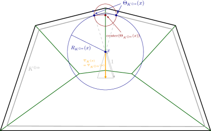
Figure 8. Pictorial overview of the definitions and notation. The set $K^{\oplus\alpha}$ is indicated in grey.

The same pentagon and medial axis as in Figures 5 and 6 with an $\alpha$-offset and with notation indicated.

We introduce the map $\operatorname{\mathcal{F}}_{K}^{\alpha}:\left(K^{\oplus\alpha}\right)^{c}\rightarrow{\mathbb{R}_{\geq 0}}$ as

(27) $$\operatorname{\mathcal{F}}_{K}^{\alpha}\underset{\text{def.}}{=}\>\operatorname{\mathcal{F}}_{K^{\oplus\alpha}}.$$

Therefore (9), (24) , (25) and (26) give us that for $x\in\left(K^{\oplus\alpha}\right)^{c}$, that is $R_{K}(x)>\alpha$, one has,

(28) $$\operatorname{\mathcal{F}}_{K}^{\alpha}(x)=\frac{R_{K}(x)-\alpha}{R_{K}(x)}\operatorname{\mathcal{F}}_{K}(x).$$

The $(\lambda,\alpha)$-medial axis of $K$, denoted $\operatorname{{ax}}_{\lambda}^{\alpha}(K)$ is the $\lambda$-medial axis of the $\alpha$-offset of $K$

$$\operatorname{{ax}}_{\lambda}^{\alpha}(K) \underset{\text{def.}}{=}\>\operatorname{{ax}}_{\lambda}(K^{\oplus\alpha})$$

(29) $$\,=\{x\in\mathbb{R}^{n}\mid\operatorname{\mathcal{F}}_{K}^{\alpha}(x)\geq\lambda\}.$$ (by (27))

We note that Lemma 8.8 extends to $(\lambda,\alpha)$-medial axis of $K$ which is therefore compact as well.

Since, for $r\geq\alpha$, the map $r\mapsto\frac{r-\alpha}{r}$ is increasing, we get from (15), Lemma 8.4, and (28) that

(30) $$t\mapsto\operatorname{\mathcal{F}}_{K}^{\alpha}(\Phi_{K}(t,x))\>\text{ is not decreasing.}$$

In fact, when $\alpha>0$, $t\mapsto R_{K}(\Phi_{K}(t,x))$ is strictly increasing as long as $\|\nabla_{K}(\Phi_{K}(t,x))\|>0$, moreover the map $t\mapsto\operatorname{\mathcal{F}}_{K}^{\alpha}(\Phi_{K}(t,x))$ is strictly increasing, which will be quantified in (LABEL:equation:FAlphaIncreaseRate) below.

The monotonicity in (30), together with the definition of $\operatorname{{ax}}_{\lambda}^{\alpha}(K)$, implies that $\operatorname{{ax}}_{\lambda}^{\alpha}(K)$ is mapped to itself under the action of the flow:

(31) $$\forall t\geq 0,\>\Phi_{K}(t,\operatorname{{ax}}_{\lambda}^{\alpha}(K))\subset\operatorname{{ax}}_{\lambda}^{\alpha}(K).$$

Observe that for $\lambda>\alpha$ one has

(32) $$x\in\operatorname{{ax}}_{\lambda}(K)\Rightarrow R_{K}(x)\geq\operatorname{\mathcal{F}}_{K}(x)\geq\lambda.$$

So if $x\in\operatorname{{ax}}_{\lambda}(K)$, we get from (28) that

$$\operatorname{\mathcal{F}}_{K}^{\alpha}(x)=\frac{R_{K}(x)-\alpha}{R_{K}(x)}\operatorname{\mathcal{F}}_{K}(x)\geq\frac{\lambda-\alpha}{\lambda}\operatorname{\mathcal{F}}_{K}(x).$$

So that,

$$x\in\operatorname{{ax}}_{\lambda}(K) \Rightarrow\operatorname{\mathcal{F}}_{K}(x)\geq\lambda\Rightarrow\operatorname{\mathcal{F}}_{K}^{\alpha}(x)\geq\frac{\lambda-\alpha}{\lambda}\lambda=\lambda-\alpha$$

$$\Rightarrow x\in\operatorname{{ax}}_{\lambda-\alpha}^{\alpha}(K).$$

This in turn implies that if $\lambda>\alpha$, one has,

(33) $$\operatorname{{ax}}_{\lambda}(K)\subset \operatorname{{ax}}_{\lambda-\alpha}^{\alpha}(K)\subset\operatorname{{ax}}_{\lambda-\alpha}(K)$$

(34) $$\operatorname{{ax}}_{\lambda}^{\alpha}(K)\subset \operatorname{{ax}}_{\lambda}(K)\subset\operatorname{{ax}}_{\lambda-\alpha}^{\alpha}(K),$$

and for any $c$ such that $0<c<1$ one has:

(35) $$\bigcup_{\lambda>0}\>\bigcup_{0<\alpha<\lambda}\operatorname{{ax}}_{\lambda}^{\alpha}(K)=\bigcup_{\lambda>0}\operatorname{{ax}}_{\lambda}^{c\lambda}(K)=\operatorname{{ax}}(K).$$

It follows from (28) and (29) that $(\lambda,\alpha)\mapsto\operatorname{{ax}}_{\lambda}^{\alpha}(K)$ is decreasing for inclusion order:

(36) $$\lambda_{1}\leq\lambda_{2},\alpha_{1}\leq\alpha_{2}\Rightarrow\operatorname{{ax}}_{\lambda_{2}}^{\alpha_{2}}(K)\subset\operatorname{{ax}}_{\lambda_{1}}^{\alpha_{1}}(K).$$

9.2. The $(\lambda,\alpha)$-medial axis is Hausdorff-stable under $\lambda$ perturbation

The purpose of this section is to show that the $(\lambda,\alpha)$-medial axis does not suffer much from instabilities. In this subsection we treat the stability with respect to $\lambda$ (Lemma 9.4 ), the following subsection is dedicated to the stability with respect to $\alpha$ (Lemma 9.5).

We start with introducing the $(\alpha,\mu)$-reach.

Definition 9.1.

For $\mu\in(0,1]$ and $\alpha\geq 0$, the $(\alpha,\mu)$-reach of $K$, denoted by $r_{\mu}^{\alpha}(K)$, is defined as:

$$r_{\mu}^{\alpha}(K)\underset{\text{def.}}{=}\>\inf\{t>\alpha,\>\chi_{K}(t)<\mu\}=\alpha+r_{\mu}(K^{\oplus\alpha}).$$

We need an easy lemma that gives a lower bound on the norm of $\|\nabla_{K}(x)\|$ for $x\in\left(K^{\oplus\alpha^{\prime}}\right)^{c}\setminus\operatorname{{ax}}_{\lambda}^{\alpha}$, for $0<\alpha^{\prime}\leq\alpha$. To be able to state the result we define,

(37) $$\tilde{\mu}_{\mu,\lambda}^{\alpha,\alpha^{\prime}}(K)\underset{\text{def.}}{=}\>\min\left(\mu,\sqrt{1-\left(\frac{\lambda}{r_{\mu}^{\alpha^{\prime}}(K)-\alpha}\right)^{2}}\right).$$

Lemma 9.2.

Let $K\subset\mathbb{R}^{n}$ be the complement of a bounded open set $K^{c}$ and $\alpha,\lambda>0$, $\mu\in(0,1]$ and $\alpha^{\prime}$ such that $0<\alpha^{\prime}\leq\alpha$ and $r_{\mu}^{\alpha^{\prime}}(K)>\alpha+\lambda$.
For any $x\in\left(K^{\oplus\alpha^{\prime}}\right)^{c}\setminus\operatorname{{ax}}_{\lambda}^{\alpha}$, one has

$$\|\nabla_{K}(x)\|\geq\tilde{\mu},$$

where

$$\tilde{\mu}=\tilde{\mu}_{\mu,\lambda}^{\alpha,\alpha^{\prime}}(K)>0.$$

Proof.

Because the lower bound $\tilde{\mu}$ is defined as a minimum over two values we distinguish two cases:

• If $R_{K}\left(x\right)<r_{\mu}^{\alpha^{\prime}}(K)$ then by definition of $r_{\mu}^{\alpha^{\prime}}$ one has
  $\|\nabla_{K}\left(x\right)\|\geq\mu$.

• If $R_{K}\left(x\right)\geq r_{\mu}^{\alpha^{\prime}}(K)$ then $R_{K^{\oplus\alpha}}(x)\geq r_{\mu}^{\alpha^{\prime}}(K)-\alpha$. Since $x\notin\operatorname{{ax}}_{\lambda}^{\alpha}$, one has $\operatorname{\mathcal{F}}_{K^{\oplus\alpha}}(x)=\operatorname{\mathcal{F}}_{\lambda}^{\alpha}(x)<\lambda$. Combining this with (12) we get,

  $$\|\nabla_{K}\left(x\right)\| =\|\nabla_{K^{\oplus\alpha}}\left(x\right)\|$$

  $$=\sqrt{1-\left(\frac{\operatorname{\mathcal{F}}_{K^{\oplus\alpha}}(x)}{R_{K^{\oplus\alpha}}(x)}\right)^{2}}$$

  $$>\sqrt{1-\left(\frac{\lambda}{r_{\mu}^{\alpha^{\prime}}(K)-\alpha}\right)^{2}}>0.$$

So that in both cases, we get:

(38) $$\|\nabla_{K}\left(x\right)\|\geq\tilde{\mu}_{\mu,\lambda}^{\alpha,\alpha^{\prime}}(K)>0.$$

∎

As observed in (Chazal and Lieutier, 2005a), the $\lambda$-medial axis seen as a function $\lambda\mapsto\operatorname{{ax}}_{\lambda}(K)$ is not continuous: $\operatorname{{ax}}_{\lambda}(K)$ may “increase” abruptly at some “singular” values of $\lambda$, even when $\lambda$ is small with respect to $\operatorname{wfs}(K)$. This is illustrated in Figures 9 and 10. This is related to the fact that, for $x\in\operatorname{{ax}}_{\lambda}(K)$, the map $t\mapsto\operatorname{\mathcal{F}}_{K}(\Phi_{K}(t,x))$ may remain constant on some intervals.

Figure 9. $\lambda\mapsto\operatorname{{ax}}_{\lambda}(K)$ is not continuous, because $K$ is non-smooth at the points $a$ and $b$.

[A curve that is smooth with the exception of two points.]A curve that is smooth with the exception of two points, $a$ and $b$, that lie directly above each other and a distance $2\tilde{\lambda}$ apart. This gives that the $\lambda$-medial axis is not continuous at $\tilde{\lambda}$.

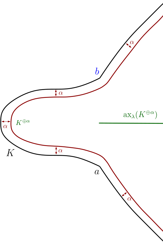
Figure 10. $\lambda\mapsto\operatorname{{ax}}_{\lambda}^{\alpha}(K)$ is continuous.

[The same curve as in the previous figure (Figure 9), but with an $\alpha$ offset. ]The same curve as in the previous figure (Figure 9), but with an $\alpha$ offset. Taking the offset removes the discontinuity.

In contrast, for $\alpha>0$, the map $\lambda\mapsto\operatorname{{ax}}^{\alpha}_{\lambda}(K)$ is continuous with respect to the Hausdorff distance, as long as $\alpha+\lambda<\operatorname{wfs}(K)$, or, more generally, as long as $\alpha+\lambda<r_{\mu}^{\alpha}(K)$ for some $\mu>0$. The continuity follows from the fact that the rate of increase of the map $t\mapsto\operatorname{\mathcal{F}}^{\alpha}_{K}(\Phi_{K}(t,x))$ is lower bounded as soon as $\operatorname{\mathcal{F}}^{\alpha}_{K}(x)>0$. More precisely, we have:

Lemma 9.3.

Let $K\subset\mathbb{R}^{n}$ be the complement of a bounded open set $K^{c}$ and $\alpha,\delta,\lambda>0$, $\mu\in(0,1]$ such that $r_{\mu}^{\alpha}(K)>\alpha+\lambda+\delta$. One has:

(39) $$\Phi_{K}\left(T,\operatorname{{ax}}_{\lambda}^{\alpha}(K)\right)\subset\operatorname{{ax}}_{\lambda+\delta}^{\alpha}(K),$$

with

$$T=\frac{R_{\max}^{2}}{\alpha\lambda\tilde{\mu}^{2}}\delta,$$

where $R_{\max}=R_{\max}(K)<\infty$ has been defined in (17). For any $x\in\operatorname{{ax}}_{\lambda}^{\alpha}(K)$, the path

$$[0,T]\ni t\rightarrow\Phi_{K}(t,x)\in\operatorname{{ax}}_{\lambda}^{\alpha}(K),$$

has length $S$ upper bounded by

$$S\leq\frac{R_{\max}^{2}}{\alpha\lambda\tilde{\mu}^{2}}\delta,$$

where $\tilde{\mu}=\tilde{\mu}_{\mu,\lambda+\delta}^{\alpha,\alpha}(K)>0$, and

(40) $$\operatorname{{ax}}_{\lambda}^{\alpha}(K)\subset\left(\operatorname{{ax}}_{\lambda+\delta}^{\alpha}(K)\right)^{\oplus S}.$$

Proof.

For $r\geq\alpha$ the map $t\mapsto\frac{r-\alpha}{r}$ is increasing, this together with (15), Lemma 8.4 and (28) yields

(41) $$\operatorname{\mathcal{F}}^{\alpha}_{K}\left(\Phi_{K}(t,x)\right)\geq\frac{R_{K}\left(\Phi_{K}(t,x)\right)-\alpha}{R_{K}\left(\Phi_{K}(t,x)\right)}\operatorname{\mathcal{F}}_{K}(x).$$

Observe that, using (15) again,

(42) $$\frac{d}{dt^{+}}\frac{R_{K}\left(\Phi_{K}(t,x)\right)-\alpha}{R_{K}\left(\Phi_{K}(t,x)\right)}=\frac{\alpha}{R_{K}\left(\Phi_{K}(t,x)\right)^{2}}\nabla_{K}\left(\Phi_{K}(t,x)\right)^{2}.$$

Consider now $T$ such that $\Phi_{K}(T,x)\notin\operatorname{{ax}}_{\lambda+\delta}^{\alpha}(K)$, and then $\operatorname{\mathcal{F}}^{\alpha}_{K}\left(\Phi_{K}(T,x)\right)<\lambda+\delta$. From (30) this gives:

$$\forall t\in[0,T],\>\operatorname{\mathcal{F}}^{\alpha}_{K}\left(\Phi_{K}(t,x)\right)<\lambda+\delta.$$

Lemma 9.2 gives a lower bound on $\|\nabla_{K}(\Phi_{K}(t,x))\|$, that is,

$$\|\nabla_{K}(\Phi_{K}(t,x))\|\geq\tilde{\mu}=\tilde{\mu}_{\mu,\lambda+\delta}^{\alpha,\alpha}(K)>0$$

and (42) then gives,

(43) $$t\in[0,T]\Rightarrow\frac{d}{dt^{+}}\frac{R_{K}\left(\Phi_{K}(t,x)\right)-\alpha}{R_{K}\left(\Phi_{K}(t,x)\right)}>\frac{\alpha\tilde{\mu}^{2}}{R_{\max}^{2}}.$$

This, thanks to Theorem 8.10, leads us to the following bound,

$$\operatorname{\mathcal{F}}^{\alpha}_{K} \left(\Phi_{K}(T,x)\right)-\operatorname{\mathcal{F}}^{\alpha}_{K}(x)$$

(by (41)) $$\geq\operatorname{\mathcal{F}}_{K}(x)\left(\frac{R_{K}\left(\Phi_{K}(T,x)\right)-\alpha}{R_{K}\left(\Phi_{K}(T,x)\right)}-\frac{R_{K}(x)-\alpha}{R_{K}(x)}\right)$$

$$=\operatorname{\mathcal{F}}_{K}(x)\int_{0}^{T}\left(\frac{d}{dt^{+}}\frac{R_{K}\left(\Phi_{K}(t,x)\right)-\alpha}{R_{K}\left(\Phi_{K}(t,x)\right)}\right)dt$$

(by (43)) $$>\operatorname{\mathcal{F}}_{K}(x)T\frac{\alpha\tilde{\mu}^{2}}{R_{\max}^{2}}.$$

Because $x\in\operatorname{{ax}}_{\lambda}^{\alpha}(K)$, $\operatorname{\mathcal{F}}^{\alpha}_{K}(x)\geq\lambda$, and (34) we find that $x\in\operatorname{{ax}}_{\lambda}(K)$. The fact that $x\in\operatorname{{ax}}_{\lambda}(K)$ in turn implies that $\operatorname{\mathcal{F}}_{K}(x)\geq\lambda$. This then yields,

$$\operatorname{\mathcal{F}}^{\alpha}_{K}\left(\Phi_{K}(T,x)\right)>\lambda+\frac{\lambda\alpha\tilde{\mu}^{2}}{R_{\max}^{2}}T.$$

We have shown that:

$$x\in\operatorname{{ax}}_{\lambda}^{\alpha}(K)\> \>\Phi_{K}(T,x)\notin\operatorname{{ax}}_{\lambda+\delta}^{\alpha}(K)$$ and

$$\Rightarrow \>\lambda+\frac{\lambda\alpha\tilde{\mu}^{2}}{R_{\max}^{2}}T<\lambda+\delta\Rightarrow T<\frac{\delta R_{\max}^{2}}{\lambda\alpha\tilde{\mu}^{2}}.$$

By contraposition we have:

$$x\in\operatorname{{ax}}_{\lambda}^{\alpha}(K)\>\text{and}\>T\geq\frac{\delta R_{\max}^{2}}{\lambda\alpha\tilde{\mu}^{2}}\Rightarrow\Phi_{K}(T,x)\in\operatorname{{ax}}_{\lambda+\delta}^{\alpha}(K).$$

Since $\forall y,\,\|\nabla_{K}(y)\|\leq 1$, one has

$$S=\operatorname{length}\left(\Phi_{K}([0,T],x\right)=\int_{0}^{T}\|\nabla_{K}\left(\Phi_{K}(t,x)\right)\|dt\leq T\leq\frac{\delta R_{\max}^{2}}{\lambda\alpha\tilde{\mu}^{2}}.$$

Since the Euclidean distance between $x\in\operatorname{{ax}}_{\lambda}^{\alpha}(K)$ and $\Phi_{K}\left(T,x\right)\in\operatorname{{ax}}_{\lambda+\delta}^{\alpha}(K)$ cannot be larger than the length of the path connecting them we get (40).

∎

Since for $\delta\geq 0$ one has $\operatorname{{ax}}_{\lambda+\delta}^{\alpha}(K)\subset\operatorname{{ax}}_{\lambda}^{\alpha}(K)$, (40) and the upper bound (22) immediately give us:

Lemma 9.4.

Let $K\subset\mathbb{R}^{n}$ be the complement of a bounded open set $K^{c}$ and $\alpha,\lambda_{\max}>0$, $\mu\in(0,1]$ such that $r_{\mu}^{\alpha}(K)>\alpha+\lambda_{\max}$. The map

$$\lambda\mapsto\operatorname{{ax}}_{\lambda}^{\alpha}(K)$$

is $\left(\frac{R_{\max}^{2}}{\alpha\lambda_{\min}\tilde{\mu}^{2}}\right)$-Lipschitz in the interval $[\lambda_{\min},\lambda_{\max}]$ for Hausdorff distance, where $R_{\max}=R_{\max}(K)<\infty$ and $\tilde{\mu}=\tilde{\mu}_{\mu,\lambda_{\max}}^{\alpha,\alpha}>0$.

9.3. The $(\lambda,\alpha)$-medial axis is Hausdorff-stable under $\alpha$ perturbation

In this subsection we complete the proof of the stability of the $(\lambda,\alpha)$-medial axis under perturbations of $\lambda$ and $\alpha$. It is not difficult to see that $\operatorname{{ax}}_{\lambda}^{\alpha+\delta}(K)\subset\operatorname{{ax}}_{\lambda}^{\alpha}(K)$ for $\delta\geq 0$. We establish that $\operatorname{{ax}}_{\lambda}^{\alpha}(K)$ is not very far from $\operatorname{{ax}}_{\lambda}^{\alpha+\delta}(K)$ by proving that $\operatorname{{ax}}_{\lambda}^{\alpha}(K)$ flows (fast enough) into $\operatorname{{ax}}_{\lambda}^{\alpha+\delta}(K)$. This is done by determining that the radius of the enclosing ball of the closest points on $K$ increases sufficiently fast.

Lemma 9.5.

Let $K\subset\mathbb{R}^{n}$ be the complement of a bounded open set $K^{c}$ and $\alpha,\lambda>0$, $\mu\in(0,1]$ if $r_{\mu}^{\alpha_{\min}}(K)>\alpha_{\max}+\lambda$. The map

$$\alpha\mapsto\operatorname{{ax}}_{\lambda}^{\alpha}(K)$$

is $\left(\frac{R_{\max}}{\alpha_{\min}\tilde{\mu}^{2}}\right)$-Lipschitz in the interval $[\alpha_{\min},\alpha_{\max}]$ for Hausdorff distance, where $\tilde{\mu}=\tilde{\mu}_{\mu,\lambda}^{\alpha_{\max},\alpha_{\min}}>0$.

Proof.

From (28) we conclude that,

$$\delta\geq 0\Rightarrow\forall x\in\left(K^{\oplus\alpha+\delta}\right)^{c},\,\operatorname{\mathcal{F}}_{K}^{\alpha}(x)\geq\operatorname{\mathcal{F}}_{K}^{\alpha+\delta}(x).$$

It follows that

(45) $$\delta\geq 0\Rightarrow\operatorname{{ax}}_{\lambda}^{\alpha+\delta}(K)\subset\operatorname{{ax}}_{\lambda}^{\alpha}(K).$$

Let us assume that for some $\mu>0$ one has $r_{\mu}^{\alpha}(K)>\alpha+\delta+\lambda$ and take $x\in\operatorname{{ax}}_{\lambda}^{\alpha}(K)$. Using Lemma 9.2, we see that

(46) $$\Phi_{K}(t,x)\notin\operatorname{{ax}}_{\lambda}^{\alpha+\delta}(K)\Rightarrow\|\nabla_{K}\left(\Phi_{K}(t,x)\right)\|>\tilde{\mu}>0,$$

where $\tilde{\mu}=\tilde{\mu}_{\mu,\lambda}^{\alpha+\delta,\alpha}(K)>0$.

It then follows from (15) that,

$$R_{K}\left(\Phi_{K}\left(\frac{R_{\max}}{\alpha\tilde{\mu}^{2}}\delta,x\right)\right) =\int_{0}^{\frac{R_{\max}}{\alpha\tilde{\mu}^{2}}\delta}\frac{d}{dt^{\prime+}}R_{K}(\Phi_{K}(t^{\prime},x))\mathrm{d}t^{\prime}+R_{K}(x)$$

$$=\int_{0}^{\frac{R_{\max}}{\alpha\tilde{\mu}^{2}}\delta}\left\|\nabla_{K}\left(\Phi_{K}(t^{\prime},x)\right)\right\|^{2}\mathrm{d}t^{\prime}+R_{K}(x)$$

(by (46)) $$>R_{K}(x)+\frac{R_{\max}}{\alpha}\delta$$

$$\geq R_{K}(x)\frac{\alpha+\delta}{\alpha}.$$

Using (28), we see

$$\operatorname{\mathcal{F}}_{K}^{\alpha+\delta} \left(\Phi_{K}\left(\frac{R_{\max}}{\alpha\tilde{\mu}^{2}}\delta,x\right)\right)$$

$$=\frac{R_{K}\left(\Phi_{K}\left(\frac{R_{\max}}{\alpha\tilde{\mu}^{2}}\delta,x\right)\right)-(\alpha+\delta)}{R_{K}\left(\Phi_{K}\left(\frac{R_{\max}}{\alpha\tilde{\mu}^{2}}\delta,x\right)\right)}\operatorname{\mathcal{F}}_{K}\left(\Phi_{K}\left(\frac{R_{\max}}{\alpha\tilde{\mu}^{2}}\delta,x\right)\right)$$

$$>\frac{R_{K}(x)\frac{\alpha+\delta}{\alpha}-(\alpha+\delta)}{R_{K}(x)\frac{\alpha+\delta}{\alpha}}\operatorname{\mathcal{F}}_{K}(x)$$

$$=\frac{R_{K}(x)-\alpha}{R_{K}(x)}\operatorname{\mathcal{F}}_{K}(x)$$

(by definition) $$=\operatorname{\mathcal{F}}_{K}^{\alpha}(x)$$

(because $$x\in\operatorname{{ax}}_{\lambda}^{\alpha} \geq\lambda,$$)

where in the second line we used that for $r\geq\alpha+\delta$, the map $r\mapsto\frac{r-(\alpha+\delta)}{r}$ is increasing, as well as the previous bound and Lemma 8.4.

With this we have shown that

(47) $$r_{\mu}^{\alpha}(K)>\alpha+\delta+\lambda\Rightarrow\Phi_{K}\left(\frac{R_{\max}}{\alpha\tilde{\mu}^{2}}\delta,\operatorname{{ax}}_{\lambda}^{\alpha}\right)\subset\operatorname{{ax}}_{\lambda}^{\alpha+\delta}(K).$$

As for Lemma 9.4, this together with (31) and (45) completes the proof of the lemma. ∎

9.4. The $(\lambda,\alpha)$-medial axis has the right homotopy type and a finite geodesic diameter

In this section, we recover that the $(\lambda,\alpha)$-medial axis preserves the homotopy type, as for the usual medial axis (Lieutier, 2004). We then prove that there exists a path of finite length between any two points in the $(\lambda,\alpha)$-medial axis, that is it has a finite geodesic diameter. Both results are again based on manipulations of the flow $\Phi_{K}$.

The next lemma gives an upper bound on the time needed for the flow $\Phi_{K}$ to map $K^{c}$ inside $\operatorname{{ax}}_{\lambda}^{\alpha}(K)$. It is instrumental for characterizing the homotopy type of $\operatorname{{ax}}_{\lambda}^{\alpha}(K)$ (Theorem 9.7) and establishing that it has finite geodesic diameter (Theorem 9.12).

Lemma 9.6.

Let $K\subset\mathbb{R}^{n}$ be the complement of a bounded open set $K^{c}$ and $\alpha\geq 0$, $\lambda>0$, $\mu\in(0,1]$ and $\alpha^{\prime}$ such that $0<\alpha^{\prime}\leq\alpha$ and $r_{\mu}^{\alpha^{\prime}}(K)>\alpha+\lambda$. Then, $\Phi_{K}\left(\frac{R_{\max}}{\tilde{\mu}^{2}},\left(K^{\oplus\alpha^{\prime}}\right)^{c}\right)\subset\operatorname{{ax}}_{\lambda}^{\alpha}(K),$ where $R_{\max}=R_{\max}(K)<\infty$ and $\tilde{\mu}=\tilde{\mu}_{\mu,\lambda}^{\alpha,\alpha^{\prime}}>0$.

Proof.

Consider $x\in\left(K^{\oplus\alpha^{\prime}}\right)^{c}$. Using (31) and Lemma 9.2 again, one finds,

$$\Phi_{K}(T,x)\notin\operatorname{{ax}}_{\lambda}^{\alpha}\Rightarrow\forall t\in[0,T],\|\nabla_{K}\left(\Phi_{K}(t,x)\right)\|>\tilde{\mu}.$$

Applying (15) as before yields,

$$\Phi_{K}(T,x)\notin\operatorname{{ax}}_{\lambda}^{\alpha}(K)$$

$$\Rightarrow R_{K}(\Phi_{K}(T,x))=\int_{0}^{T}\frac{d}{dt^{+}}R_{K}(\Phi_{K}(t,x))\mathrm{d}t+R_{K}(\Phi_{K}(0,x))>T\tilde{\mu}^{2}.$$

Since $R_{K}(\Phi_{K}(T,x))\leq R_{\max}$ one gets,

$$\Phi_{K}(T,x)\notin\operatorname{{ax}}_{\lambda}^{\alpha}(K)\Rightarrow T\tilde{\mu}^{2}<R_{\max}\Rightarrow T<\frac{R_{\max}}{\tilde{\mu}^{2}}.$$

The contraposition gives,

$$\Phi_{K}\left(\frac{R_{\max}}{\tilde{\mu}^{2}},x\right)\in\operatorname{{ax}}_{\lambda}^{\alpha}(K).$$

∎

We now define the map

$$H:[0,1]\times\left(K^{\oplus\alpha^{\prime}}\right)^{c} \rightarrow\left(K^{\oplus\alpha^{\prime}}\right)^{c}$$

$$(t,x) \mapsto\Phi_{K}\left(\frac{R_{\max}}{\tilde{\mu}^{2}}t,x\right)=H(t,x).$$

Lemma 9.6, (31), and the natural inclusion $\operatorname{{ax}}_{\lambda}^{\alpha}(K)\subset\left(K^{\oplus\alpha^{\prime}}\right)^{c}$ together imply that $H$ gives a homotopy equivalence between $\left(K^{\oplus\alpha^{\prime}}\right)^{c}$ and $\operatorname{{ax}}_{\lambda}^{\alpha}(K)$, as it satisfies Definition 8.1. Since, by (19),

$$r<\operatorname{wfs}(K)\Rightarrow\exists\mu>0,\,\textrm{such that }r_{\mu}^{\alpha}(K)\geq r,$$

one sees that:

Theorem 9.7.

Let $K\subset\mathbb{R}^{n}$ be the complement of a bounded open set $K^{c}$, $\alpha\geq 0$, $\lambda>0$ and $\alpha^{\prime}$ such that $0<\alpha^{\prime}\leq\alpha$ and $r_{\mu}^{\alpha^{\prime}}(K)>\alpha+\lambda$ then $\operatorname{{ax}}_{\lambda}^{\alpha}(K)$ has the same homotopy type as $\left(K^{\oplus\alpha^{\prime}}\right)^{c}$.

Pushing a path $\gamma$ along the flow $\Phi$, while keeping its endpoints fixed, will be instrumental in several subsequent proofs. We introduce therefore a specific notation for such pushed paths.

Definition 9.8 (Pushed paths).

Let $K\subset\mathbb{R}^{n}$ be a closed set, $\gamma:[0,1]\rightarrow K^{c}$ a rectifiable path and $T\geq 0$. The path $\gamma$ pushed along a time $T$ by the flow $\Phi_{K}$ with fixed end points, denoted ${\gamma}^{\left[T\right]_{K}}$ is the path ${\gamma}^{\left[T\right]_{K}}:[0,1]\rightarrow K^{c}$ from $\gamma(0)$ to $\gamma(1)$ defined by:

$${\gamma}^{\left[T\right]_{K}}(t)=\begin{cases}\Phi_{K}(3tT,\gamma(0))&\textrm{if}\quad t\in[0,1/3]\\ \Phi_{K}(T,\gamma(3t-1))&\textrm{if}\quad t\in[1/3,2/3]\\ \Phi_{K}((3(1-t)T,\gamma(1))&\textrm{if}\quad t\in[2/3,1].\end{cases}$$

The next simple lemma says that ${\gamma}^{\left[T\right]_{K}}(t)$ is rectifiable and allows to upper bound path lengths in several subsequent proofs (Theorems 9.12 and 11.1, Lemmas 9.14 and 9.15 ).

Lemma 9.9.

Let $K\subset\mathbb{R}^{n}$ be a closed set and $\alpha>0$. Let $\gamma:[0,1]\rightarrow\left(K^{\oplus\alpha}\right)^{c}$ be a rectifiable path with length $L(\gamma)$ and $T\geq 0$. ${\gamma}^{\left[T\right]_{K}}$ is rectifiable and has length $L\left({\gamma}^{\left[T\right]_{K}}\right)$ upper bounded by:

$$L\left({\gamma}^{\left[T\right]_{K}}\right)\leq 2\,T+L(\gamma)e^{\frac{T}{\alpha}}.$$

Proof.

Since the norm of $\nabla_{K}(x)$ is upper bounded by $1$, ${\gamma}^{\left[T\right]_{K}}$ is $3$-Lipschitz on the first and third intervals $[0,1/3]$ and $[2/3,1]$ so that the length of each of these parts is upper bounded by $T$.

Because $\mathrm{im}(\gamma)$ is included in $\left(K^{\oplus\alpha}\right)^{c}$, the length of ${\gamma}^{\left[T\right]_{K}}\left([1/3,2/3]\right)$ is bounded by

$$L(\gamma)e^{\frac{T}{\alpha}}.$$

This follows, because (16) can be applied to arbitrary small subdivisions of $\mathbf{\gamma}$, the bound on the expansion factor extends to the length of the curve through the definition of the length of rectifiable curves. ∎

The next theorem shows that connected components of $(\lambda,\alpha)$-medial axes have finite geodesic diameter. In particular, geodesic distances inside connected components of $(\lambda,\alpha)$-medial axes are finite, and are realized by minimal paths.

Before we can go into the precise statement we need to introduce some notation. For a Borel set $X\subset\mathbb{R}^{n}$ we denote by $\operatorname{Vol}(X)$ its $n$-Lebesgue measure, or volume. We write $V_{n}=\operatorname{Vol}(\operatorname{\mathbb{B}}^{n}(0,1))$ for the volume of the unit $n$-ball, $V_{n}=\frac{\pi^{\frac{n}{2}}}{\Gamma\left(\frac{n}{2}+1\right)},$ where $\Gamma$ is the Euler Gamma function, see for example (Duistermaat and Kolk, 2004, page 622).

Remark 9.10.

Thanks to Theorem 9.7, connected components of $\operatorname{{ax}}_{\lambda}^{\alpha}(K)$ are in one to one correspondance with connected components of $\left(K^{\oplus\alpha}\right)^{c}$. For this reason, the next statements related to geodesic diameters and Gromov-Hausdorff distance assumes $\left(K^{\oplus\alpha}\right)^{c}$ connected without real loss of generality.

While any connected open subset of $\mathbb{R}^{n}$ is path-wise connected (Sutherland, 2009, Proposition 12.25), some connected open bounded subset may not have a finite geodesic diameter. We’ll illustrate this in the following example. Let

$$S=\left\{(x,y)\in\mathbb{R}^{2}\big{|}\>0<x<1,\>-\frac{1}{2}+\sin\frac{1}{x}<y<\frac{1}{2}+\sin\frac{1}{x}\right\}$$

Observe that $S$ is indeed a connected, bounded, open subset of $\mathbb{R}^{2}$ with infinite geodesic diameter. Moreover, for some $\alpha>1$, taking

$$K=\Big{\{}(x,y,z)\in\mathbb{R}^{3}\big{|}\>(x,y)\notin S\>\>\>\text{and}\>\>\>d\big{(}(x,y,z),\>S\times\{0\}\big{)}\geq\alpha\Big{\}},$$

we get that the open bounded set $\left(K^{\oplus\alpha}\right)^{c}$ deform retracts by vertical projection on $S\times\{0\}$ along trajectories of small length $h<1$. Thanks to this vertical deformation retract we have that $d_{GH}(\left(K^{\oplus\alpha}\right)^{c},S)\leq 2h$. More precisely the argument goes as follows: We have that

$$\left(K^{\oplus\alpha}\right)^{c}=\left\{(x,y,z)\middle|(x,y)\in S\textrm{ and }|z|<\bar{h}(x,y)\right\},$$

with $\bar{h}(x,y)\leq h\leq 1$. It follows by concatenating a geodesic $S$ with vertical line segments, that

$$d((x_{1},y_{1},z_{1}),(x_{2},y_{2},z_{2}))\leq d((x_{1},y_{1}),(x_{2},y_{2}))+2h.$$

Here we wrote $(x_{1},y_{1},z_{1}),(x_{2},y_{2},z_{2})$ for elements of $\left(K^{\oplus\alpha}\right)^{c}$ and $(x_{1},y_{1}),(x_{2},y_{2})$ for the elements of $S$ with the same first two coordinates. Conversely, $d((x_{1},y_{1}),(x_{2},y_{2}))\leq d((x_{1},y_{1},z_{1}),(x_{2},y_{2},z_{2}))$ because for any rectifiable curve $\gamma(t)\subset\mathbb{R}^{3}$ we have $L(\pi_{\mathbb{R}^{2}}(\gamma(t)))\leq L(\gamma(t))$, where $\pi_{\mathbb{R}^{2}}$ denotes the projection onto $\mathbb{R}^{2}$. It follows from the bound $d_{GH}(\left(K^{\oplus\alpha}\right)^{c},S)\leq 2h$ that $\left(K^{\oplus\alpha}\right)^{c}$ also has infinite geodesic diameter. So to be the complement of an offset does not imply finite geodesic diameter either.

However, we have the following:

Lemma 9.11.

Let $K\subset\mathbb{R}^{n}$ be the complement of a bounded, open set $K^{c}$. Assume there are $\mu>0$ and $\alpha>\alpha^{\prime}>0$ such that $r_{\mu}^{\alpha^{\prime}}(K)>\alpha$.

Then, if $\left(K^{\oplus\alpha}\right)^{c}$ is connected it has finite geodesic diameter. In particular, if for some $z\in\mathbb{R}^{n}$ and $R_{\operatorname{bound}}>0$, one has $K^{c}\subset\operatorname{\mathbb{B}}(z,R_{\operatorname{bound}})$, then:

$${\operatorname{GeoDiameter}}\left(\left(K^{\oplus\alpha}\right)^{c}\right)\leq 2\frac{\alpha-\alpha^{\prime}}{\mu}$$

$$+2\left(\left(\frac{4R_{\operatorname{bound}}}{\alpha-\alpha^{\prime}}\right)^{n}+1\right)(\alpha-\alpha^{\prime})e^{\frac{\alpha-\alpha^{\prime}}{\alpha\mu}}.$$

This diameter is bounded by constructing a very dense graph inside the set $\left(K^{\oplus\alpha^{\prime}}\right)^{c}$ and bounding the distance between any two points in the graph. The result then follows by pushing this path inside $\left(K^{\oplus\alpha}\right)^{c}$.

of Lemma 9.11.

Since $\left(K^{\oplus\alpha}\right)^{c}$ is compact, we can cover it by a finite number of open balls $\left(\operatorname{\mathbb{B}}^{\circ}(y_{i},\frac{\alpha-\alpha^{\prime}}{2})\right)_{i\in I_{0}}$, where $I_{0}$ is a finite set and $y_{i}\in\left(K^{\oplus\alpha}\right)^{c}$. It is possible to extract an $\varepsilon$-net $\{y_{i},i\in I\}$ from $\{y_{i},i\in I_{0}\}$, that is $I\subset I_{0}$ and

(48) $$\left(K^{\oplus\alpha}\right)^{c}\subset\bigcup_{i\in I}\operatorname{\mathbb{B}}^{\circ}\left(y_{i},\alpha-\alpha^{\prime}\right)\subset\left(K^{\oplus\alpha^{\prime}}\right)^{c},$$

with

(49) $$i,j\in I\>\text{and}\>i\neq j\Rightarrow\operatorname{\mathbb{B}}\left(y_{i},\frac{\alpha-\alpha^{\prime}}{4}\right)\cap\operatorname{\mathbb{B}}\left(y_{i},\frac{\alpha-\alpha^{\prime}}{4}\right)=\emptyset.$$

Let us denote the cardinality of $I$ by $N$. Since by (49) the balls $\operatorname{\mathbb{B}}\left(y_{i},\frac{\alpha-\alpha^{\prime}}{4}\right)$ are disjoint and $\cup_{i\in I}\operatorname{\mathbb{B}}\left(y_{i},\frac{\alpha-\alpha^{\prime}}{4}\right)\subset K^{c}\subset\operatorname{\mathbb{B}}(z,R_{\operatorname{bound}})$ one has

(50) $$N\leq\frac{\operatorname{Vol}(\operatorname{\mathbb{B}}(z,R_{\operatorname{bound}}))}{\operatorname{Vol}\left(\operatorname{\mathbb{B}}\left(0,\frac{\alpha-\alpha^{\prime}}{4}\right)\right)}\leq\left(\frac{4R_{\operatorname{bound}}}{\alpha-\alpha^{\prime}}\right)^{n}.$$

Let $G$ be the graph with one vertex for each $y_{i}\in\{1,\ldots,N\}$ and one edge for each pair $(i,j)$ such that $\operatorname{\mathbb{B}}^{\circ}(y_{i},\alpha-\alpha^{\prime})\cap\operatorname{\mathbb{B}}^{\circ}(y_{j},\alpha-\alpha^{\prime})\neq\emptyset$. This graph is connected as otherwise, from (48), $\left(K^{\oplus\alpha}\right)^{c}$ would be the disjoint union of two non-empty disjoint open sets, which would contradict its connectedness.

Consider $x,x^{\prime}\in\left(K^{\oplus\alpha}\right)^{c}$ and let $k,k^{\prime}$ be such that $x\in\operatorname{\mathbb{B}}^{\circ}(y_{k},\alpha-\alpha^{\prime})$ and $x^{\prime}\in\operatorname{\mathbb{B}}^{\circ}(y_{k^{\prime}},\alpha-\alpha^{\prime})$. We define a piecewise linear path $\mathbf{P}$ from $x$ to $x^{\prime}$ as follows. First let $y_{k}=y_{i_{0}}\ldots y_{i_{M}}=y_{k^{\prime}}$ a shortest path between $y_{k}$ and $y_{k^{\prime}}$ in the graph $G$. We define the piecewise linear path $\mathbf{P}$ in $\left(K^{\oplus\alpha^{\prime}}\right)^{c}$ as the concatenation of the segments

$$[xy_{i_{0}}],[y_{i_{0}}y_{i_{1}}],\ldots,[y_{i_{M-1}}y_{i_{M}}],[y_{i_{M}},x^{\prime}].$$

The length of $P$ is then lower bounded: $L(\mathbf{P})\leq 2(N+1)(\alpha-\alpha^{\prime})$. By definition of $r_{\mu}^{\alpha^{\prime}}(K)$, since $r_{\mu}^{\alpha^{\prime}}(K)>\alpha$ we have that $\|\nabla_{K}(x)\|\geq\mu$ for $x\in\left(K^{\oplus\alpha^{\prime}}\right)^{c}\setminus\left(K^{\oplus\alpha}\right)^{c}$, so that ${P}^{\left[\frac{\alpha-\alpha^{\prime}}{\mu}\right]_{K}}\subset\left(K^{\oplus\alpha}\right)^{c}$. Applying Lemma 9.9 we get:

$$L\left({P}^{\left[\frac{\alpha-\alpha^{\prime}}{\mu}\right]_{K}}\right)\leq 2\frac{\alpha-\alpha^{\prime}}{\mu}+L(P)e^{\frac{\alpha-\alpha^{\prime}}{\alpha\mu}}.$$

∎

Theorem 9.12.

Let $K\subset\mathbb{R}^{n}$ be the complement of a bounded, open set $K^{c}$ and $\alpha,\lambda>0$ such that $r_{\mu}^{\alpha}(K)>\alpha+\lambda$ and assume $\left(K^{\oplus\alpha}\right)^{c}$ to be connected with finite geodesic diameter:

$${\operatorname{GeoDiameter}}\left(\left(K^{\oplus\alpha}\right)^{c}\right)<\infty.$$

Then $\operatorname{{ax}}_{\lambda}^{\alpha}(K)$ is a geodesic space with finite geodesic diameter given by (51) below. More precisely, if $x,x^{\prime}\in\operatorname{{ax}}_{\lambda}^{\alpha}(K)$, then there exists a path $\gamma:[0,1]\rightarrow\operatorname{{ax}}_{\lambda}^{\alpha}(K)$ of minimal length such that $\gamma(0)=x$ and $\gamma(1)=x^{\prime}$. This path satisfies,

$$\operatorname{length}(\gamma) \leq{\operatorname{GeoDiameter}}(\operatorname{{ax}}_{\lambda}^{\alpha}(K))$$

(51) $$\leq 2\frac{R_{\max}}{\tilde{\mu}^{2}}+{\operatorname{GeoDiameter}}\left(\left(K^{\oplus\alpha}\right)^{c}\right)e^{\frac{R_{\max}}{\alpha\tilde{\mu}^{2}}},$$

where $R_{\max}=R_{\max}(K)$, $\tilde{\mu}=\tilde{\mu}_{\mu,\lambda}^{\alpha,\frac{\alpha}{2}}$. The length $\operatorname{length}(\gamma)$ is the geodesic distance between $x$ and $x^{\prime}$ in $\operatorname{{ax}}_{\lambda}^{\alpha}(K)$.

The proof follows by pushing paths into the medial axis, using Lemma 9.9.

Proof.

Consider $x,x^{\prime}\in\operatorname{{ax}}_{\lambda}^{\alpha}(K)\subset\left(K^{\oplus\alpha}\right)^{c}$ and $\Gamma$ a path in $\left(K^{\oplus\alpha}\right)^{c}$ from $x$ to $x^{\prime}$ with length upper bounded by
${\operatorname{GeoDiameter}}\left(\left(K^{\oplus\alpha}\right)^{c}\right)$.

As in Lemma 9.3 we set $\tilde{\mu}=\tilde{\mu}_{\mu,\lambda}^{\alpha,\alpha}$. Using Definition 9.8 we consider now the path ${\Gamma}^{\left[\frac{R_{\max}}{\tilde{\mu}^{2}}\right]_{K}}$ with end points $x$ and $x^{\prime}$. Because $\Gamma$ is included in $\left(K^{\oplus\alpha}\right)^{c}$, Lemma 9.9 gives:

(52) $$L\left({\Gamma}^{\left[\frac{R_{\max}}{\tilde{\mu}^{2}}\right]_{K}}\right)\leq 2\frac{R_{\max}}{\tilde{\mu}^{2}}+L(\Gamma)e^{\frac{R_{\max}}{\alpha\tilde{\mu}^{2}}}$$

Due to (31), ${\Gamma}^{\left[\frac{R_{\max}}{\tilde{\mu}^{2}}\right]_{K}}\left([0,1/3]\right)$ and ${\Gamma}^{\left[\frac{R_{\max}}{\tilde{\mu}^{2}}\right]_{K}}\left([2/3,1]\right)$ are inside $\operatorname{{ax}}_{\lambda}^{\alpha}(K)$. As a consequence of Lemma 9.6, ${\Gamma}^{\left[\frac{R_{\max}}{\tilde{\mu}^{2}}\right]_{K}}\left([1/3,2/3]\right)$ also lies in $\operatorname{{ax}}_{\lambda}^{\alpha}(K)$.

This upper bound (52) on the length is independent of $x,x^{\prime}\in\operatorname{{ax}}_{\lambda}^{\alpha}(K)$ and it therefore gives an upper bound on the geodesic diameter of $\operatorname{{ax}}_{\lambda}^{\alpha}(K)$.

It is known that if a finite length path exists between two points in a compact subset of Euclidean space, then there exists a path of minimal length, see the second paragraph of Part III, Section 1: Die Existenz geodätischer Bogen in metrischen Räumen, in (Menger, 1930). ∎

As a consequence of Lemma 9.11 and Theorem 9.12 we get:

Corollary 9.13.

Let $K\subset\mathbb{R}^{n}$ be the complement of a bounded, open set $K^{c}$, $\alpha>\alpha^{\prime}>0$ and $\lambda>0$ such that $r_{\mu}^{\alpha^{\prime}}(K)>\alpha+\lambda$ and assume $\left(K^{\oplus\alpha}\right)^{c}$ to be connected.

Then $\operatorname{{ax}}_{\lambda}^{\alpha}(K)$ is a geodesic space with finite geodesic diameter.

9.5. The $(\lambda,\alpha)$-medial axis is Gromov-Hausdorff-stable under $\lambda$ perturbation

Thanks to Theorem 9.12, $\operatorname{{ax}}_{\lambda}^{\alpha}(K)$ is a geodesic space with finite length inside connected components. Equipped with this geodesic distance $\operatorname{{ax}}_{\lambda}^{\alpha}(K)$ is a metric space which is stable under $\lambda$ perturbation in the following sense:

Lemma 9.14.

Let $K\subset\mathbb{R}^{n}$ be the complement of a bounded, open set $K^{c}$ and $\alpha,\delta,\lambda>0$, $\mu\in(0,1]$ such that, for some $\alpha^{\prime}<\alpha$ one has $r_{\mu}^{\alpha^{\prime}}(K)>\alpha+\lambda+\delta$ and $\left(K^{\oplus\alpha}\right)^{c}$ is connected.

Then, the map $\lambda\mapsto\operatorname{{ax}}_{\lambda}^{\alpha}(K)$ is locally Lipschitz for the Gromov-Hausdorff distance with respect to the intrinsic metric.

More precisely, one has

$$d_{\textrm{GH}}(\operatorname{{ax}}_{\lambda+\delta}^{\alpha}(K),\operatorname{{ax}}_{\lambda}^{\alpha}(K))\leq 2T+D\left(e^{\frac{T}{\alpha}}-1\right)=O\left(\delta\right),$$

with

$$T=\frac{R_{\max}^{2}}{\alpha\lambda\tilde{\mu}^{2}}\delta.$$

and $D<\infty$ is the geodesic diameter of $\operatorname{{ax}}_{\lambda}^{\alpha}(K)$.

The core of the proof consists of pushing the geodesics in $\operatorname{{ax}}_{\lambda}^{\alpha}$ into $\operatorname{{ax}}_{\lambda+\delta}^{\alpha}$, which is again achieved by the flow. The other properties we need to verify to establish a bound on the Gromov-Hausdorff distance are relatively straightforward.

Proof.

The value of the geodesic diameter $D$ is given by Theorem 9.12. In order to upper bound the Gromov-Hausdorff distance between $\operatorname{{ax}}_{\lambda+\delta}^{\alpha}(K)$ and $\operatorname{{ax}}_{\lambda}^{\alpha}(K)$ we use Definition 8.7.

Consider the relation $\mathcal{R}\subset\operatorname{{ax}}_{\lambda}^{\alpha}(K)\times\operatorname{{ax}}_{\lambda+\delta}^{\alpha}(K)$ defined by:

$$\mathcal{R}=\left\{(x_{1},x_{2})\in\operatorname{{ax}}_{\lambda}^{\alpha}(K)\times\operatorname{{ax}}_{\lambda+\delta}^{\alpha}(K),\>\exists t\in[0,T],\,x_{2}=\Phi_{K}(t,x_{1})\right\},$$

where $T=\frac{R_{\max}^{2}}{\alpha\lambda\tilde{\mu}^{2}}\delta$.

We have to check the two conditions of Definition 8.7. Recall that, by Lemma 9.3, one has

$$\Phi_{K}\left(T,\operatorname{{ax}}_{\lambda}^{\alpha}(K)\right)\subset\operatorname{{ax}}_{\lambda+\delta}^{\alpha}(K)\subset\operatorname{{ax}}_{\lambda}^{\alpha}(K).$$

Condition (1): $\mathcal{R}$ is surjective.

This condition follows because, if $x_{1}\in\operatorname{{ax}}_{\lambda}^{\alpha}(K)$ then $\Phi_{K}(T,x_{1})\in\operatorname{{ax}}_{\lambda+\delta}^{\alpha}(K)$, thanks to Lemma 9.3. This is in turn equivalent to $\left(x_{1},\Phi_{K}(T,x_{1})\right)\in\mathcal{R}$. Conversely, if $x_{2}\in\operatorname{{ax}}_{\lambda+\delta}^{\alpha}(K)$, then $x_{2}\in\operatorname{{ax}}_{\lambda}^{\alpha}(K)$ and $(x_{2},x_{2})\in\mathcal{R}$ since $\Phi_{K}(0,x_{2})=x_{2}$.

Condition (2): The bound on the distance distortion.

Consider $(x_{1},x_{2}),(x_{1}^{\prime},x_{2}^{\prime})\in\mathcal{R}$, with $x_{2}=\Phi_{K}(t,x_{1})$ and $x_{2}^{\prime}=\Phi_{K}(t^{\prime},x_{1}^{\prime})$ with $t,t^{\prime}\in[0,T]$. Denote by $d_{1}$ and $d_{2}$ the respective intrinsic distances in $\operatorname{{ax}}_{\lambda}^{\alpha}(K)$ and $\operatorname{{ax}}_{\lambda+\delta}^{\alpha}(K)$. By Theorem 9.7, since $\left(K^{\oplus\alpha}\right)^{c}$ is connected (which is equivalent to be path-wise connected for an open set), $\operatorname{{ax}}_{\lambda}^{\alpha}(K)$ is path-wise connected and $x_{1}$ and $x_{1}^{\prime}$ are in the same connected component of $\operatorname{{ax}}_{\lambda}^{\alpha}(K)$. Thanks to Theorem 9.12, $d_{1}(x_{1},x_{1}^{\prime})<\infty$  and there is a path $\gamma_{1}:[0,1]\rightarrow\operatorname{{ax}}_{\lambda}^{\alpha}(K)$ such that $d_{1}(x_{1},x_{1}^{\prime})=L(\gamma_{1})$. Thanks to Lemma 9.9, the path ${\gamma_{1}}^{\left[T\right]_{K}}$ has length upper bounded by $2\,T+L(\gamma_{1})e^{\frac{T}{\alpha}}$.

By Definition 9.8, one has ${\gamma_{1}}^{\left[T\right]_{K}}\left(\frac{t}{3T}\right)=x_{2}$ and ${\gamma_{1}}^{\left[T\right]_{K}}\left(1-\frac{t^{\prime}}{3T}\right)=x_{2}^{\prime}$. Moreover, (30) and (39) yields

$${\gamma_{1}}^{\left[T\right]_{K}}\left(\left[\frac{t}{3T},1-\frac{t^{\prime}}{3T}\right]\right)\subset\operatorname{{ax}}_{\lambda}^{\alpha}(K),$$

so that ${\gamma_{1}}^{\left[T\right]_{K}}\left(\left[\frac{t}{3T},1-\frac{t^{\prime}}{3T}\right]\right)$ is a path from $x_{2}$ to $x_{2}^{\prime}$ inside $\operatorname{{ax}}_{\lambda+\delta}^{\alpha}(K)$ and its length is therefore lower bounded by $d_{2}(x_{2},x_{2}^{\prime})$. It follows that

$$d_{2}(x_{2},x_{2}^{\prime}) \leq L\left({\gamma_{1}}^{\left[T\right]_{K}}\left(\left[\frac{t}{3T},1-\frac{t^{\prime}}{3T}\right]\right)\right)$$

$$\leq L\left({\gamma_{1}}^{\left[T\right]_{K}}\right)\leq 2\,T+d_{1}(x_{1},x_{1}^{\prime})e^{\frac{T}{\alpha}},$$

so that

(53) $$d_{2}(x_{2},x_{2}^{\prime})-d_{1}(x_{1},x_{1}^{\prime})\leq 2\,T+d_{1}(x_{1},x_{1}^{\prime})\left(e^{\frac{T}{\alpha}}-1\right)\leq 2\,T+D\left(e^{\frac{T}{\alpha}}-1\right).$$

Since $\operatorname{{ax}}_{\lambda+\delta}^{\alpha}(K)$ is connected, there is a path $\gamma_{2}:[0,1]\rightarrow\operatorname{{ax}}_{\lambda+\delta}^{\alpha}(K)$ such that $d_{2}(x_{2},x_{2}^{\prime})=L(\gamma_{2})$.

Consider now the path $\Gamma:[0,1]\rightarrow\operatorname{{ax}}_{\lambda}^{\alpha}(K)$ defined as:

$$\Gamma(u)=\begin{cases}\Phi_{K}(3ut,x_{1})&\textrm{if}\quad u\in[0,1/3]\\ \gamma_{2}(3u-1))&\textrm{if}\quad u\in[1/3,2/3]\\ \Phi_{K}((3(1-u)t^{\prime},x_{1}^{\prime})&\textrm{if}\quad u\in[2/3,1].\end{cases}$$

Here we used that $\operatorname{{ax}}_{\lambda+\delta}^{\alpha}(K)\subset\operatorname{{ax}}_{\lambda}^{\alpha}$ for $u\in[1/3,2/3]$. By (30) $\Gamma$ is a path from $x_{1}$ to $x_{1}^{\prime}$ inside $\operatorname{{ax}}_{\lambda}^{\alpha}(K)$ so that

$$d_{1}(x_{1},x_{1}^{\prime})\leq L\left(\Gamma\right)\leq 2\,T+L\left(\gamma_{2}\right)=2\,T+d_{2}(x_{2},x_{2}^{\prime})$$

and with (53) we get as required

$$\left|d_{2}(x_{2},x_{2}^{\prime})-d_{1}(x_{1},x_{1}^{\prime})\right|\leq 2\,T+D\left(e^{\frac{T}{\alpha}}-1\right).$$

Note that by Corollary 9.13 (using the assumption $r_{\mu}^{\alpha^{\prime}}(K)>\alpha+\lambda+\delta$) the geodesic diameter $D$ of $\operatorname{{ax}}_{\lambda}^{\alpha}(K)$ is finite. ∎

9.6. The $(\lambda,\alpha)$-medial axis is Gromov-Hausdorff-stable under $\alpha$ perturbation

Using almost identical arguments as in the previous section we also get the Gromov-Hausdorff stability with respect the offset $\alpha$.

Lemma 9.15.

Let $K\subset\mathbb{R}^{n}$ be the complement of a bounded open set $K^{c}$ and $\alpha,\delta,\lambda>0$, $\mu\in(0,1]$ such that, for some $\alpha^{\prime}<\alpha$ one has $r_{\mu}^{\alpha^{\prime}}(K)>\alpha+\lambda+\delta$ and $\left(K^{\oplus\alpha}\right)^{c}$ is connected. Then, the map

$$\alpha\mapsto\operatorname{{ax}}_{\lambda}^{\alpha}(K)$$

is locally Lipschitz for the Gromov-Hausdorff distance with respect to the intrinsic metric.

More precisely, one has

$$d_{\textrm{GH}}(\operatorname{{ax}}_{\lambda}^{\alpha+\delta}(K),\operatorname{{ax}}_{\lambda}^{\alpha}(K))\leq 2T+D\left(e^{\frac{T}{\alpha}}-1\right)=O\left(\delta\right),$$

with

$$T=\frac{R_{\max}}{\alpha\tilde{\mu}^{2}}\delta,$$

and $D<\infty$ is the geodesic diameter of $\operatorname{{ax}}_{\lambda}^{\alpha}(K)$.

Proof.

This is similar to Section 9.5 using (47) instead of (39). ∎

10. Hausdorff stability of the $(\lambda,\alpha)$-medial axis under Hausdorff perturbation of $K$

In this section, we prove one of the main stability theorems of this paper, namely stability in the Hausdorff sense of the $(\lambda,\alpha)$-medial axis under Hausdorff perturbations of $K$. This requires some further results on the flow that are proven in the first subsections, while the main result is proven in the final subsection. As in the previous section we use the flow to establish our main result, namely the Hausdorff stability. Intuitively this may seem straightforward, because near the medial axis the flow we follow points towards the medial axis. However, establishing that the flow is fast enough requires a number of technical estimates. Firstly we need that the distance to the closest points ($R_{K}$) increases sufficiently fast as we follow the flow. This is proven in Section 10.1. Based on this result we can prove that

• Points close to $\operatorname{{ax}}_{\lambda}^{\alpha}(K)$ flow inside it after a short amount of time (Section 10.2).

• If you perturb $K$ into $K^{\prime}$ (near in Hausdorff distance) then $\operatorname{{ax}}^{\alpha}_{\lambda}(K^{\prime})$ flows into $\operatorname{{ax}}_{\lambda-\delta}^{\alpha}(K)$ after a short amount of time (Section 10.3).

The bound on the Hausdorff distance is finally established based on this and Lemma 9.3.

10.1. A lower bound on $R_{K}$ along the flow trajectories

The technical result that underpins the lemma in this section is the Volterra integral inequality, as discussed in Section 8.7.

Lemma 10.1.

Let $K\subset\mathbb{R}^{n}$ be the complement of a bounded open set $K^{c}$, $\alpha\geq 0$ and $\lambda>0$. Consider $y\in\left(K^{\oplus\alpha}\right)^{c}\setminus\operatorname{{ax}}_{\lambda}^{\alpha}(K)$ and denote by $s\mapsto y(s)$ the trajectory of $t\mapsto\Phi_{K}\left(t,y\right)$, parametrized by arc length. We stress that $y(0)=y$. Assume that $R_{K}(y)-\alpha>\lambda$ and that for some $S>0$ one has

$$y(S)\notin\operatorname{{ax}}_{\lambda}^{\alpha}(K),$$

then

$$\left(R_{K}(y(S))-\alpha\right)^{2}\geq(S_{0}+S)^{2}+\lambda^{2},$$

where $S_{0}>0$ is defined as

$$S_{0}^{2}=\left(R_{K}(y)-\alpha\right)^{2}-\lambda^{2}.$$

Proof.

We define the map $R_{0}:[0,S]\rightarrow\mathbb{R}$ as

$$R_{0}(s)=\sqrt{(S_{0}+s)^{2}+\lambda^{2}}{+\alpha}.$$

We need to prove that $R_{K}(y(s))\geq R_{0}(s)$, which we’ll do by means of Theorem 8.12. By definition of $S_{0}$, one has $R_{0}(0)=R_{K}(y)$. For $s\in[0,S]$ we get

$$\frac{d}{ds}(R_{0}(s)-\alpha)^{2}=2(S_{0}+s).$$

It follows that

$$\frac{d}{ds}R_{0}(s) =\frac{(S_{0}+s)}{R_{0}(s)-\alpha}$$

$$=\frac{\sqrt{(R_{0}(s)-\alpha)^{2}-\lambda^{2}}}{R_{0}(s)-\alpha}$$

$$=\sqrt{1-\left(\frac{\lambda}{R_{0}(s)-\alpha} \right)^{2}}$$

and thus we have the Volterra integral inequality,

$$R_{0}(s)=R_{0}(0)+\int_{0}^{s}k(R_{0}(\tau))\mathrm{d}\tau,$$

where the kernel $k$ is

$$k(x)=\sqrt{1-\left(\frac{\lambda}{x-\alpha} \right)^{2}}.$$

Combining (13), and (15) gives

$$\frac{d}{ds^{+}}R_{K}(y(s)) =\left\|\nabla_{K}\left(y(s)\right)\right\|$$

$$=\sqrt{1-\left(\frac{\operatorname{\mathcal{F}}^{\alpha}(y(s)) }{R_{K}(y(s))-\alpha} \right)^{2}},$$

see also (Chazal and Lieutier, 2005a, Equation (5)). Because $R_{K}(y(s))$ is Lipschitz, Theorem 8.10 yields that

$$R_{K}(y(s)) =R_{K}(y)+\int_{0}^{s}\sqrt{1-\left(\frac{\operatorname{\mathcal{F}}^{\alpha}(y(\tau)) }{R_{K}(y(\tau))-\alpha} \right)^{2}}\mathrm{d}\tau$$

$$=R_{0}(0)+\int_{0}^{s}\sqrt{1-\left(\frac{\operatorname{\mathcal{F}}^{\alpha}(y(\tau)) }{R_{K}(y(\tau))-\alpha} \right)^{2}}\mathrm{d}\tau.$$

By assumption $y(S)\notin\operatorname{{ax}}_{\lambda}^{\alpha}$, so (30) implies that $s\leq S\Rightarrow\operatorname{\mathcal{F}}^{\alpha}(y(s))<\lambda$. Moreover, for sufficiently small $0<\delta^{\prime}\leq S$ we can assume that $\operatorname{\mathcal{F}}^{\alpha}(y(s))\leq\lambda^{\prime}<\lambda$, for $s\in[0,\delta]$, by Lemma 8.4. This means that $R_{K}(y(s))$ satisfies the following integral inequality of Volterra type,

$$R_{K}(y(s)) \geq R_{0}(0)+\int_{0}^{s}\sqrt{1-\left(\frac{\lambda}{R_{K}(y(\tau))-\alpha} \right)^{2}}\mathrm{d}\tau$$

$$=R_{0}(0)+\int_{0}^{s}k(R_{K}(y(\tau)))\mathrm{d}\tau,$$

where the equality occurs only when $s=0$. We note that, because $R_{K}(y)-\alpha>\lambda>0$ and $R_{K}(y)$ is monotone,

$$\frac{d}{dx}k(x)=\frac{\lambda^{2}}{(x-\alpha)^{3}\sqrt{1-\frac{\lambda^{2}}{(x-\alpha)^{2}}}}\geq 0$$

on the domain and thus the kernel is monotone. Because $R_{K}(y(s))$ is 1-Lipschitz in $s$ and we can assume that there is some $\delta^{\prime}\leq\delta$ such that for all $s\in(0,\delta^{\prime})$, we have $R_{K}(y(s))>R_{0}(s)$. In fact $\delta^{\prime}$ is determined by the condition

$$\sqrt{1-\left(\frac{\lambda^{\prime}}{R_{0}(0)-\delta^{\prime}-\alpha} \right)^{2}} \geq\sqrt{1-\left(\frac{\lambda}{R_{0}(0)+\delta^{\prime}-\alpha} \right)^{2}}$$

$$\frac{\lambda^{\prime}}{R_{0}(0)-\delta^{\prime}-\alpha} \leq\frac{\lambda}{R_{0}(0)+\delta^{\prime}-\alpha}.$$

The result is now a direct consequence of the application of Theorem 8.12. ∎

10.2. Points close to $\operatorname{{ax}}_{\lambda}^{\alpha}(K)$ flow inside it after a short time

Lemma 10.2.

Let $K\subset\mathbb{R}^{n}$ be the complement of a bounded open set $K^{c}$ and $\alpha>0$, $\mu>0$ and $\lambda>0$, such that $r_{\mu}^{\alpha}(K)>\alpha+\lambda$. Then, if $\delta<\lambda$ and $\epsilon<\min\left(2\alpha,\frac{\left(2\lambda-\delta\right)\delta}{8R_{\max}}\right)$ one has

$$\Phi_{K}\left(\frac{8R_{\max}^{2}}{\left(2\lambda-\delta\right)\delta\tilde{\mu}}\>\epsilon\,,\>\operatorname{{ax}}_{\lambda}^{\alpha}(K)^{\oplus\epsilon}\right)\subset\operatorname{{ax}}_{\lambda-\delta}^{\alpha}(K),$$

where $R_{\max}=R_{\max}(K)<\infty$ and $\tilde{\mu}=\tilde{\mu}_{\mu,\lambda}^{\alpha,\alpha}>0$. Moreover, for $y\in\operatorname{{ax}}_{\lambda}^{\alpha}(K)^{\oplus\epsilon}$, the length of the trajectory $\Phi_{K}\left(\left[0,\frac{8R_{\max}^{2}}{\left(2\lambda-\delta\right)\delta\tilde{\mu}}\>\epsilon\right],y\right)$ is upper bounded by

$$\frac{8R_{\max}^{2}}{\left(2\lambda-\delta\right)\delta}\>\epsilon.$$

Proof.

Consider $y\in\operatorname{{ax}}_{\lambda}^{\alpha}(K)^{\oplus\epsilon}$ and $a\in\operatorname{{ax}}_{\lambda}^{\alpha}(K)$ such that $\|y-a\|\leq\epsilon$. Denote by $s\mapsto y(s)$ the trajectory of $t\mapsto\Phi_{K}\left(t,y\right)$, parametrized by arc length, so that $y(0)=y$. Let us now assume that for some $s>0$ one has

$$y(s)\notin\operatorname{{ax}}_{\lambda-\delta}^{\alpha}(K).$$

Since $a\in\operatorname{{ax}}_{\lambda}^{\alpha}(K)$ (34) yields that $a\in\operatorname{{ax}}_{\lambda}(K)$. The bound (32) gives that $R_{K}(a)\geq F_{K}(a)$. This together with (29) and (28) gives

(54) $$R_{K}(a)-\alpha\geq\lambda.$$

By the conditions of the theorem we have $\epsilon<\delta$ and $\|y-a\|\leq\epsilon$, (54) therefore implies

(55) $$R_{K}(y)-\alpha>\lambda-\delta,$$

by the triangle inequality. This means that the condition of Lemma 10.1 are satisfied.

We can then apply Lemma 10.1 with $\lambda$ replaced by $\lambda-\delta$, which gives us

(56) $$\left(R_{K}(y(s))-\alpha\right)^{2}\geq(S_{0}+s)^{2}+(\lambda-\delta)^{2},$$

where

(57) $$S_{0}^{2}=\left(R_{K}(y)-\alpha\right)^{2}-(\lambda-\delta)^{2}.$$

Since $R_{K}(a)-\alpha\geq\lambda$ there is $S_{a}\geq 0$ such that

(58) $$S_{a}^{2}+\lambda^{2}=\left(R_{K}(a)-\alpha\right)^{2}.$$

We recall Lemma 4.15 of (Lieutier, 2004). The correspondence between the notation is the following:

We pick $\mathcal{O}$ to be equal to $\left(K^{\oplus\alpha}\right)^{c}$, $x$ to be $a$ and $y$ to be $y(s)$, then $\mathscr{R}(x)$ is $R_{K}(a)-\alpha$, $\mathscr{R}(y)$ is $R_{K}(y(s))-\alpha$, and $\mathscr{F}(x)$ is $\operatorname{\mathcal{F}}_{K}^{\alpha}(a)$. So that the inequality of Lemma 4.15 of (Lieutier, 2004) reads (using our notation):

$$(R_{K}(y(s))-\alpha)^{2}$$

$$\leq(R_{K}(a)-\alpha)^{2}+2\|y(s)-a\|\sqrt{(R_{K}(a)-\alpha)^{2}-\operatorname{\mathcal{F}}_{K}^{\alpha}(a)^{2}}+\|y(s)-a\|^{2}.$$

Using (58) we have:

$$(R_{K}(y(s))-\alpha)^{2}$$

$$\leq\lambda^{2}+S_{a}^{2}+2\|y(s)-a\|\sqrt{(R_{K}(a)-\alpha)^{2}-\operatorname{\mathcal{F}}_{K}^{\alpha}(a)^{2}}+\|y(s)-a\|^{2}.$$

and since $\operatorname{\mathcal{F}}_{K}^{\alpha}(a)\geq\lambda$ one has, using (58) again,

$$\sqrt{(R_{K}(a)-\alpha)^{2}-\operatorname{\mathcal{F}}_{K}^{\alpha}(a)^{2}}\leq S_{a}$$

and

$$(R_{K}(y(s))-\alpha)^{2}\leq(S_{a}+\|y(s)-a\|)^{2}+\lambda^{2}.$$

Because $\|y(s)-a\|\leq\|y-a\|+\|y(s)-y\|\leq\epsilon+s$, we get

(59) $$(R_{K}(y(s))-\alpha)^{2}\leq(S_{a}+s+\epsilon)^{2}+\lambda^{2}.$$

Combining this with (56) yields,

$$(S_{a}+s+\epsilon)^{2}+\lambda^{2}\geq(S_{0}+s)^{2}+(\lambda-\delta)^{2},$$

which can be rewritten as

(60) $$2(S_{0}-S_{a}-\epsilon)s\leq(2\lambda-\delta)\delta-\left(S_{0}^{2}-S_{a}^{2}\right)+\left(2S_{a}+\epsilon\right)\,\epsilon.$$

To recover an upper bound on $s$ from (60), we need a lower bound on $(S_{0}-S_{a}-\epsilon)$ and an upper bound on the right hand side of the previous inequality, that is an upper bound on $(2\lambda-\delta)\delta-\left(S_{0}^{2}-S_{a}^{2}\right)+\left(2S_{a}+\epsilon\right)\,\epsilon$.

From (57) and (58) we get

$$S_{0}^{2}-S_{a}^{2} = \left(R_{K}(y)-\alpha\right)^{2}-(\lambda-\delta)^{2}-\left(R_{K}(a)-\alpha\right)^{2}+\lambda^{2}$$

$$= \left(R_{K}(y)-\alpha\right)^{2}-\left(R_{K}(a)-\alpha\right)^{2}+(2\lambda-\delta)\delta,$$

so that,

(61) $$S_{0}^{2}-S_{a}^{2}-(2\lambda-\delta)\delta=\left(R_{K}(y)-\alpha\right)^{2}-\left(R_{K}(a)-\alpha\right)^{2}.$$

Since $|R_{K}(y)-R_{K}(a)|<\epsilon$ we get,

$$|\left(R_{K}(y)-\alpha\right)^{2}-\left(R_{K}(a)-\alpha\right)^{2}|<|R_{K}(y)+R_{K}(a)-2\alpha|\,\epsilon\leq 2R_{\max}\,\epsilon,$$

where we used that $R_{K}(y),R_{K}(a)\leq R_{\max}$ by definition of $R_{\max}$ and $\alpha\leq R_{\max}$. Now (61), in turn gives,

(62) $$|(2\lambda-\delta)\delta-(S_{0}^{2}-S_{a}^{2})|<2R_{\max}\,\epsilon$$

or, equivalently

(63) $$(2\lambda-\delta)\delta-2R_{\max}\epsilon<S_{0}^{2}-S_{a}^{2}<(2\lambda-\delta)\delta+2R_{\max}\,\epsilon.$$

With the assumption $\epsilon<\frac{(2\lambda-\delta)\delta}{8R_{\max}}$, which gives $2R_{\max}\,\epsilon<\frac{1}{4}(2\lambda-\delta)\delta$, (63) yields,

(64) $$0<\frac{3}{4}(2\lambda-\delta)\delta<S_{0}^{2}-S_{a}^{2}<\frac{5}{4}(2\lambda-\delta)\delta.$$

This in turn implies that

$$S_{0}-S_{a}=\frac{S_{0}^{2}-S_{a}^{2}}{S_{0}+S_{a}}>\frac{3}{4}\frac{\left(2\lambda-\delta\right)\delta}{S_{0}+S_{a}}.$$

Combining (58) and (57) one has $S_{0}+S_{a}<2R_{\max}$ and using again $\epsilon<\frac{\left(2\lambda-\delta\right)\delta}{8R_{\max}}$ we get

(65) $$S_{0}-S_{a}-\epsilon>\frac{3}{8}\frac{\left(2\lambda-\delta\right)\delta}{R_{\max}}-\epsilon>\frac{\left(2\lambda-\delta\right)\delta}{4R_{\max}}.$$

We have from $\epsilon<2\alpha$ and (58) that $2S_{a}+\epsilon<2(S_{a}+\alpha)\leq 2R_{\max}$. Therefore (60) together with (62) gives us

$$2(S_{0}-S_{a}-\epsilon)s <2R_{\max}\,\epsilon+\left(2S_{a}+\epsilon\right)\,\epsilon$$

(66) $$\leq 4R_{\max}\epsilon.$$

Remark 10.3.

Note that the assumption $\epsilon<2\alpha$ is not really necessary as, here, we could merely upper bound $\epsilon$ by $R_{\max}$, so that $2S_{a}+\epsilon<3R_{\max}$ and we would get $5R_{\max}\epsilon$ instead of $4R_{\max}\epsilon$ as upper bound in (66).

Equations (65) and (66) gives us

$$s<\frac{8R_{\max}^{2}}{\left(2\lambda-\delta\right)\delta}\>\epsilon$$

We have obtained this inequality by assuming $y(s)\notin\operatorname{{ax}}_{\lambda-\delta}^{\alpha}$. By contraposition we get

$$y\left(\frac{8R_{\max}^{2}}{\left(2\lambda-\delta\right)\delta}\>\epsilon\right)\in\operatorname{{ax}}_{\lambda-\delta}^{\alpha}.$$

This proves the last statement of the lemma that upper bounds the length of the trajectory. Since by Lemma 9.2, as long as $y(s)\notin\operatorname{{ax}}_{\lambda-\delta}^{\alpha}$ the modulus of the right derivative of $t\mapsto\Phi_{K}\left(t,y\right)$, which is $\frac{ds}{dt}=\|\nabla_{K}\left(\Phi_{K}\left(t,y\right)\right)\|$, is lower bounded by $\tilde{\mu}$ we get, still using Theorem 8.10, the first statement of the lemma. ∎

Remark 10.4.

While we do not need it in subsequent proofs, thanks to remark 10.3, we could omit the condition $\epsilon<2\alpha$ in Lemma 10.2, so that the lemma holds as well without this condition and then also for $\alpha=0$, that is for the $\lambda$-medial axis, at the mild price of a larger constant, replacing the flow time $\frac{8R_{\max}^{2}}{\left(2\lambda-\delta\right)\delta\tilde{\mu}}\>\epsilon$ by $\frac{10R_{\max}^{2}}{\left(2\lambda-\delta\right)\delta\tilde{\mu}}\>\epsilon$.

10.3. Flow to the medial axis after a perturbation of the set $K$.

We write $d_{H}(C_{1},C_{2})$ for the Hausdorff distance between two compact sets $C_{1},C_{2}\subset\mathbb{R}^{n}$.

Lemma 10.5.

Let $K,K^{\prime}\subset\mathbb{R}^{n}$ be complements of bounded open sets $K^{c}$ and $K^{\prime c}$ and $\alpha\geq 0$ ,$\mu>0$, $\lambda>0$, such that $r_{\mu}^{\alpha}(K)>\alpha+\lambda$.

If $d_{H}(K,K^{\prime})<\epsilon$ then, if $\delta<\lambda$ and $\epsilon<\frac{\left(2\lambda-\delta\right)\delta}{8R_{\max}}$ one has:

$$\Phi_{K}\left(\frac{8R_{\max}^{2}}{\left(2\lambda-\delta\right)\delta\tilde{\mu}}\>\epsilon\,,\>\operatorname{{ax}}_{\lambda}^{\alpha}(K^{\prime})\right)\subset\operatorname{{ax}}_{\lambda-\delta}^{\alpha}(K),$$

where $R_{\max}={\max\{R_{\max}(K),R_{\max}(K^{\prime})\}}<\infty$ and $\tilde{\mu}=\tilde{\mu}_{\mu,\lambda}^{\alpha,\alpha}>0$.

Moreover, for $y\in\operatorname{{ax}}_{\lambda}^{\alpha}(K^{\prime})$, the length of the trajectory
$\Phi_{K}\left(\left[0,\frac{8R_{\max}^{2}}{\left(2\lambda-\delta\right)\delta\tilde{\mu}}\>\epsilon\right],y\right)$ is upper bounded by

$$\frac{8R_{\max}^{2}}{\left(2\lambda-\delta\right)\delta}\>\epsilon.$$

Proof.

The proof is similar to the proof of Lemma 10.2, except that now we start with a point in $\operatorname{{ax}}_{\lambda}^{\alpha}(K^{\prime})$ and flow to $\operatorname{{ax}}_{\lambda-\delta}^{\alpha}(K)$. We consider $y\in\operatorname{{ax}}_{\lambda}^{\alpha}(K^{\prime})$. Denote by $s\mapsto y(s)$ the trajectory of $t\mapsto\Phi_{K}\left(t,y\right)$, parametrized by arc length, so that $y(0)=y$. Assume that for some $s>0$ one has:

$$y(s)\notin\operatorname{{ax}}_{\lambda-\delta}^{\alpha}{(K)}$$

Recall that $d_{H}(K,K^{\prime})<\epsilon$ implies that

(67) $$\left|R_{K^{\prime}}(x)-R_{K}(x)\right|<\epsilon,$$

for all $x$. Similarly to (54), once again has $y\in\operatorname{{ax}}_{\lambda}^{\alpha}(K^{\prime})\Rightarrow R_{K^{\prime}}(y)-\alpha>\lambda\Rightarrow R_{K}(y)-\alpha>\lambda-\epsilon$. Moreover due to the hypothesis of the lemma one has $\epsilon<\delta$, so one sees,

(55) $$R_{K}(y)-\alpha>\lambda-\delta.$$

As in the proof of Lemma 10.2 we can apply Lemma 10.1 with $\lambda$ replaced by $\lambda-\delta$, which gives us,

(68) $$\left(R_{K}(y(s))-\alpha\right)^{2}\geq(S_{0}+s)^{2}+(\lambda-\delta)^{2},$$

where:

(69) $$S_{0}^{2}=\left(R_{K}(y)-\alpha\right)^{2}-(\lambda-\delta)^{2}.$$

Since $y\in\operatorname{{ax}}_{\lambda}^{\alpha}(K^{\prime})$, $R_{K^{\prime}}(y)-\alpha\geq\lambda$ and there is $S_{y}\geq 0$ such that

(70) $$S_{y}^{2}=\left(R_{K^{\prime}}(y)-\alpha\right)^{2}-\lambda^{2}.$$

Again following the same steps as in the proof of Lemma 10.2, we use Lemma 4.15 of (Lieutier, 2004) to see that,

(71) $$\left(R_{K^{\prime}}(y(s))-\alpha\right)^{2}\leq(S_{y}+\|y(s)-y\|)^{2}+\lambda^{2}.$$

Because $y(s)$ is parametrized by arc length, we have $\|y(s)-y\|\leq s$, which together with (67) yields,

(72) $$\left(R_{K}(y(s))-\epsilon-\alpha\right)^{2}\leq(S_{y}+s)^{2}+\lambda^{2}.$$

Subtracting (68) from (72) yields,

$$0\leq (S_{y}+s)^{2}-(S_{0}+s)^{2}+\lambda^{2}-(\lambda-\delta)^{2}+\left(R_{K}(y(s))-\alpha\right)^{2}$$

$$-\left(R_{K}(y(s))-\epsilon-\alpha\right)^{2},$$

which can be rewritten (in two steps) as,

$$0\leq(S_{y}+s)^{2}-(S_{0}+s)^{2}+\left(2\lambda-\delta\right)\delta+\left(2R_{K}(y(s))-2\alpha-\epsilon\right)\,\epsilon$$

(73) $$2\left(S_{0}-S_{y}\right)s\leq\left(2\lambda-\delta\right)\delta-\left(S_{0}^{2}-S_{y}^{2}\right)+2R_{\max}\,\epsilon.$$

Again as in the proof of Lemma 10.2, combining (69) and (70) gives us

$$\left|\left(2\lambda-\delta\right)\delta-\left(S_{0}^{2}-S_{y}^{2}\right)\right| =\left|\left(R_{K^{\prime}}(y)-\alpha\right)^{2}-\left(R_{K}(y)-\alpha\right)^{2}\right|$$

$$=\left(R_{K}(y)+R_{K^{\prime}}(y)-2\alpha\right)|R_{K}(y)-R_{K^{\prime}}(y)|$$

(by (67)) $$\leq\left(R_{K}(y)+R_{K^{\prime}}(y)-2\alpha\right)\,\epsilon$$

(74) $$\leq 2R_{\max}\,\epsilon,$$

and (73) gives

(75) $$\left(S_{0}-S_{y}\right)s\leq 2R_{\max}\,\epsilon.$$

Since $\epsilon<\frac{\left(2\lambda-\delta\right)\delta}{8R_{\max}}$ , (74) yields,

$$\frac{3}{4}\left(2\lambda-\delta\right)\delta<S_{0}^{2}-S_{y}^{2}<\frac{5}{4}\left(2\lambda-\delta\right)\delta$$

and

$$S_{0}-S_{y}=\frac{S_{0}^{2}-S_{y}^{2}}{S_{0}+S_{y}}>\frac{3}{4}\frac{\left(2\lambda-\delta\right)\delta}{S_{0}+S_{y}}>\frac{\left(2\lambda-\delta\right)\delta}{4R_{\max}},$$

where we used that (69) implies that $S_{0}\leq R_{\max}$, and (70) implies $S_{y}\leq R_{\max}$. With (75) we get:

$$s<\frac{8R_{\max}}{\left(2\lambda-\delta\right)\delta}\,\epsilon$$

and we conclude exactly as in the proof of Lemma 10.2 ∎

Remark 10.6.

The previous lemma can be interpreted as a stability result with respect to the one-sided Hausdorff distance. Moreover, the lemma applies when $\alpha=0$, in which case the statement can be compared to Theorem 3 of (Chazal and Lieutier, 2005a). Theorem 3 of (Chazal and Lieutier, 2005a) says that the $\lambda$-medial axis is $\frac{1}{2}$-Hölder stable in the following sense: If $d_{H}(K,K^{\prime})<\epsilon$, then for $x\in\operatorname{{ax}}_{\lambda}(K^{\prime})$ there is $y\in ax_{\lambda-\delta}(K)$ with $\|y-x\|=O(\epsilon^{\frac{1}{2}})$. In other words the one sided Hausdorff distance between $\operatorname{{ax}}_{\lambda}(K^{\prime})$ and $\operatorname{{ax}}_{\lambda}(K)$ is $O(\epsilon^{\frac{1}{2}})$. Lemma 10.5 proves the stronger linear bound $\|y-x\|=O(\epsilon)$. The effect of a translation on $K$ shows that one cannot expect a bound better than linear.

The proofs of Theorem 3 in (Chazal and Lieutier, 2005a) and Lemma 10.5 are based on the same idea. However, here we get a better bound by using the lower bound on $R_{K}(y(S))$ given by Lemma 10.1 which is tighter than the one used in (Chazal and Lieutier, 2005a).

10.4. Hausdorff distance between $\operatorname{{ax}}_{\lambda}^{\alpha}(K^{\prime})$ and $\operatorname{{ax}}_{\lambda}^{\alpha}(K)$

Combining Lemmas 10.5 and 9.3 allows to give a more symmetric statement.

Lemma 10.7.

Let $K,K^{\prime}\subset\mathbb{R}^{n}$ be complements of a bounded open sets $K^{c}$ and $K^{\prime c}$ and $\alpha>0$, $\mu>0$, $\lambda>0$, such that $r_{\mu}^{\alpha}(K)>\alpha+\lambda$. If

$$d_{H}(K,K^{\prime})<\epsilon,$$

and, if $\delta=2\sqrt{\alpha\tilde{\mu}\epsilon}<\lambda$, and $\epsilon<\min\left(\frac{\left(2\lambda-\delta\right)\delta}{8R_{\max}},\frac{\lambda^{2}}{16\alpha\tilde{\mu}}\right)$ then,

$$\Phi_{K}\left(C\epsilon^{\frac{1}{2}}\,,\>\operatorname{{ax}}_{\lambda}^{\alpha}(K^{\prime})\right)\subset\operatorname{{ax}}_{\lambda}^{\alpha}(K),$$

where $R_{\max}=\max\{R_{\max}(K),R_{\max}(K^{\prime})\}<\infty$ , $\tilde{\mu}=\tilde{\mu}_{\mu,\lambda}^{\alpha,\alpha}(K)>0$, and $C$ is defined as

(76) $$C=\frac{22}{3}\frac{R_{\max}^{2}}{\alpha^{\frac{1}{2}}\tilde{\mu}^{\frac{3}{2}}\lambda}.$$

Moreover, if one has also symmetrically $r_{\mu}^{\alpha}(K),r_{\mu}^{\alpha}(K^{\prime})>\alpha+\lambda$ and $R_{\max}=\max\left(R_{\max}(K),R_{\max}(K^{\prime})\right)$, and $\tilde{\mu}=\min\left(\tilde{\mu}_{\mu,\lambda}^{\alpha,\alpha}(K),\tilde{\mu}_{\mu,\lambda}^{\alpha,\alpha}(K^{\prime})\right)$ we have

(77) $$d_{H}\left(\operatorname{{ax}}_{\lambda}^{\alpha}(K),\operatorname{{ax}}_{\lambda}^{\alpha}(K^{\prime})\right)<C\epsilon^{\frac{1}{2}}.$$

Proof.

We first flow $\operatorname{{ax}}_{\lambda}^{\alpha}(K^{\prime})$ into $\operatorname{{ax}}_{\lambda-\delta}^{\alpha}(K)$, and then we flow from $\operatorname{{ax}}_{\lambda-\delta}^{\alpha}(K)$ to $\operatorname{{ax}}_{\lambda}^{\alpha}(K)$. Indeed these Lemmas 10.5 and 9.3 give that if $K,K^{\prime}\subset\mathbb{R}^{n}$ are complements of a bounded open sets $K^{c}$ and $K^{\prime c}$ and $\alpha>0$, $\mu>0$, $\lambda>0$, are such that $r_{\mu}^{\alpha}(K)>\alpha+\lambda$ and $d_{H}(K,K^{\prime})<\epsilon$ then for $0<\delta<\lambda$ and $\epsilon<\frac{\left(2\lambda-\delta\right)\delta}{8R_{\max}}$ one has,

(78) $$\Phi_{K}\left(\frac{R_{\max}^{2}}{\alpha(\lambda-\delta)\tilde{\mu}^{2}}\delta+\frac{8R_{\max}^{2}}{\left(2\lambda-\delta\right)\delta\tilde{\mu}}\>\epsilon\,,\>\operatorname{{ax}}_{\lambda}^{\alpha}(K^{\prime})\right)\subset\operatorname{{ax}}_{\lambda}^{\alpha}(K),$$

where we use (14) and $R_{\max}=R_{\max}(K)<\infty$ and $\tilde{\mu}=\tilde{\mu}_{\mu,\lambda}^{\alpha,\alpha}>0$.

Here we still have to choose a value of $\delta$ that minimizes the first argument of $\Phi_{K}$ in (78), that is,

(79) $$\delta\mapsto\frac{R_{\max}^{2}}{\alpha(\lambda-\delta)\tilde{\mu}^{2}}\delta+\frac{8R_{\max}^{2}}{\left(2\lambda-\delta\right)\delta\tilde{\mu}}\>\epsilon.$$

To this end we first observe that when $\epsilon$ is small, the value of $\delta$ that minimizes, (79) is small. When $\delta$ is small (79) is well approximated by

(80) $$\delta\mapsto\frac{R_{\max}^{2}}{\alpha\lambda\tilde{\mu}^{2}}\delta+\frac{4R_{\max}^{2}}{\lambda\delta\tilde{\mu}}\>\epsilon.$$

The value of $\delta$ that minimizes (80) is

(81) $$\delta=2\sqrt{\alpha\tilde{\mu}\epsilon}.$$

We now substitute (81) in (79). If we also observe that if $\epsilon<\frac{\lambda^{2}}{16\alpha\tilde{\mu}}$, (81) gives $\delta<\lambda/2$ and thus $2\lambda-\delta>3/2\lambda$ and $\lambda-\delta>1/2\lambda$ we find the following upper bound

$$\frac{R_{\max}^{2}}{\alpha(\lambda-\delta)\tilde{\mu}^{2}}\delta+\frac{8R_{\max}^{2}}{\left(2\lambda-\delta\right)\delta\tilde{\mu}}\>\epsilon<\frac{22}{3}\frac{R_{\max}^{2}}{\alpha^{\frac{1}{2}}\tilde{\mu}^{\frac{3}{2}}\lambda}\epsilon^{\frac{1}{2}}.$$

∎

Remark 10.8.

The symmetric condition $r_{\mu}^{\alpha}(K),r_{\mu}^{\alpha}(K^{\prime})>\alpha+\lambda$ can be replaced by a condition on $K$ only. More precisely, in the limit where some $\delta$ tends to zero as $d_{H}(K,K^{\prime})\rightarrow 0$ we have that $r_{\mu}^{\alpha-\delta}(K)>\alpha+\lambda+\delta$ implies $r_{\mu}^{\alpha}(K),r_{\mu}^{\alpha}(K^{\prime})>\alpha+\lambda$ , see (Chazal et al., 2009, Theorem 3.4) where also the dependencies of $\delta$ and $d_{H}(K,K^{\prime})$ are made precise.

Lemma 10.9.

Let $K\subset\mathbb{R}^{n}$ be the complement of a bounded open set $K^{c}$ and $\alpha>0$, $\mu>0$ and $\lambda>0$, such that $r_{\mu}^{\alpha}(K)>\alpha+\lambda$. Then, if $\delta=2\sqrt{\alpha\tilde{\mu}\epsilon}<\lambda$ and $\epsilon<\min\left(2\alpha,\frac{\left(2\lambda-\delta\right)\delta}{8R_{\max}},\frac{\lambda^{2}}{16\alpha\tilde{\mu}}\right)$ one has

$$\Phi_{K}\left(C\epsilon^{\frac{1}{2}}\,,\>\left(\operatorname{{ax}}_{\lambda}^{\alpha}(K)\right)^{\oplus\epsilon}\right)\subset\operatorname{{ax}}_{\lambda}^{\alpha}(K),$$

where $R_{\max}=R_{\max}(K)<\infty$, $\tilde{\mu}=\tilde{\mu}_{\mu,\lambda}^{\alpha,\alpha}(K)>0$, and $C$ is defined by (76).

Proof.

The proof is identical to the proof of Lemma 10.7, however this this time we combine Lemmas 10.2 and 9.3 to achieve the more symmetric statement. We note that we choose the same optimal value for $\delta$ from (81). ∎

11. Gromov-Hausdorff stability of the $(\lambda,\alpha)$-medial axis under Hausdorff perturbation of $K$

Figure 11. Illustration of the proof of Theorem 11.1. The path $\Gamma$, concatenation of $\sigma_{aa^{\prime}}$, $\gamma^{\prime}$ and $\sigma_{b^{\prime}b}$, is pushed through the flow $\Phi_{K}$ into a path ${\Gamma}^{\left[C^{\frac{3}{2}}\epsilon^{\frac{1}{4}}\right]_{K}}$ that realizes a path in $\operatorname{{ax}}_{\lambda}^{\alpha}(K)$ between $a$ and $b$.

The pushing of a path on one $(\lambda,\alpha)$-medial axis onto another $(\lambda,\alpha)$-medial axis.

In this section, we bound the Gromov-Hausdorff distance between the $(\lambda,\alpha)$-medial axis of a set $K$ and the medial axis of perturbation of the set, where the perturbation is small in the Hausdorff sense. Gromov-Hausdorff distance is understood to be with respect to the intrinsic distance on the medial axis, that is the metric on the space $\operatorname{{ax}}_{\lambda}^{\alpha}(K)$ is the metric induced by the geodesic distance on the set. As we have seen in Section 9.4 this metric is well defined.

We assume that we are in the symmetric setting, that is the conditions of Lemma 10.7 are satisfied. We assume moreover that $K^{c}$ and $(K^{\prime})^{c}$ are connected.

Figure 11 illustrates the idea of the proof of Theorem 11.1. Consider the pairs

$$(a,a^{\prime}),(b,b^{\prime})\in\mathcal{R}=\left\{(x,x^{\prime})\in\operatorname{{ax}}_{\lambda}^{\alpha}(K)\times\operatorname{{ax}}_{\lambda}^{\alpha}(K^{\prime}),\|x-x^{\prime}\|<C\epsilon^{\frac{1}{2}}\right\}.$$

In order to compare the length of a geodesic $\gamma$ from $a$ to $b$ to the length of a geodesic $\gamma^{\prime}$ from $a^{\prime}$ to $b^{\prime}$ (left), we first create a path $\Gamma$ (middle), concatenation of $\gamma$ with two straight segments $\sigma_{aa^{\prime}}$ and $\sigma_{b^{\prime}b}$. Then $\Gamma$ is “pushed” (right) along the flow $\Phi_{K}$, which, after a “time” $t=\mathcal{O}\big{(}\epsilon^{\frac{1}{4}}\big{)}$, belongs to $\operatorname{{ax}}_{\lambda}^{\alpha}(K)$. The pushed path can then be shown to be not much longer than the path $\gamma^{\prime}$.

Theorem 11.1.

Let $K,K^{\prime}\subset\mathbb{R}^{n}$ be complements of bounded open sets $K^{c},(K^{\prime})^{c}$, $\alpha>0$, $\mu>0$ and $\lambda>0$, such that, for some $\alpha^{\prime}<\alpha$ one has $r_{\mu}^{\alpha^{\prime}}(K)>\alpha+\lambda$ and $r_{\mu}^{\alpha^{\prime}}(K^{\prime})>\alpha+\lambda$, and $\left(K^{\oplus\alpha}\right)^{c}$ and $\left(K^{\prime\oplus\alpha}\right)^{c}$ are connected. Denote $R_{\max}=\max\left(R_{\max}(K),R_{\max}(K^{\prime})\right)$, and $\tilde{\mu}=\min\left(\tilde{\mu}_{\mu,\lambda}^{\alpha,\alpha}(K),\tilde{\mu}_{\mu,\lambda}^{\alpha,\alpha}(K^{\prime})\right)$.

Assume that $d_{H}(K,K^{\prime})<\epsilon$. If

$$\epsilon<\min\left(\frac{\lambda^{2}\alpha\tilde{\mu}}{16R_{\max}^{2}},\frac{\lambda^{2}}{16\alpha\tilde{\mu}},\frac{9\lambda^{4}\alpha\tilde{\mu}^{3}}{400R_{\max}^{4}},\left(\frac{2\alpha}{C}\right)^{2},\left(\frac{\lambda^{2}\alpha\tilde{\mu}}{16R_{\max}^{2}C}\right)^{2},\left(\frac{\lambda^{2}}{16\alpha\tilde{\mu}C}\right)^{2}\right),$$

then the Gromov-Hausdorff distance between $\operatorname{{ax}}_{\lambda}^{\alpha}(K)$ and $\operatorname{{ax}}_{\lambda}^{\alpha}(K^{\prime})$ with respect to the intrinsic metric is upper bounded by

$$2C^{\frac{3}{2}}\epsilon^{\frac{1}{4}}+2C\epsilon^{\frac{1}{2}}e^{\frac{C^{\frac{3}{2}}\epsilon^{\frac{1}{4}}}{\alpha}}+D\left(e^{\frac{C^{\frac{3}{2}}\epsilon^{\frac{1}{4}}}{\alpha}}-1\right)=O\left(\epsilon^{\frac{1}{4}}\right),$$

where

$$C=\frac{22}{3}\frac{R_{\max}^{2}}{\alpha^{\frac{1}{2}}\tilde{\mu}^{\frac{3}{2}}\lambda}$$

and

$$D =\max\left({\operatorname{GeoDiameter}}(\operatorname{{ax}}_{\lambda}^{\alpha}(K)),{\operatorname{GeoDiameter}}(\operatorname{{ax}}_{\lambda}^{\alpha}(K^{\prime}))\right)<\infty.$$

Proof.

In order to lower bound the Gromov-Hausdorff distance between $\operatorname{{ax}}_{\lambda}^{\alpha}(K)$ and $\operatorname{{ax}}_{\lambda}^{\alpha}(K^{\prime})$ under the assumptions of Lemma 10.7 we use Definition 8.7.

Consider the relation $\mathcal{R}\subset\operatorname{{ax}}_{\lambda}^{\alpha}(K)\times\operatorname{{ax}}_{\lambda}^{\alpha}(K^{\prime})$ defined by:

(82) $$\mathcal{R}=\left\{(x,x^{\prime})\in\operatorname{{ax}}_{\lambda}^{\alpha}(K)\times\operatorname{{ax}}_{\lambda}^{\alpha}(K^{\prime}),\|x-x^{\prime}\|<C\epsilon^{\frac{1}{2}}\right\},$$

where $C$ is defined by (76).

We know from Lemma 10.7 that this relation is surjective, which means that for any $x\in\operatorname{{ax}}_{\lambda}^{\alpha}(K)$ there is $x^{\prime}\in\operatorname{{ax}}_{\lambda}^{\alpha}(K^{\prime})$ such that $(x,x^{\prime})\in\mathcal{R}$ and, reciprocally, if $x^{\prime}\in\operatorname{{ax}}_{\lambda}^{\alpha}(K^{\prime})$ there is $x\in\operatorname{{ax}}_{\lambda}^{\alpha}(K)$ such that $(x,x^{\prime})\in\mathcal{R}$.

Consider $(a,a^{\prime}),(b,b^{\prime})\in\mathcal{R}$. Since $K^{c}$ and $(K^{\prime})^{c}$ are connected, Theorem 9.12 yields that there are paths $\gamma:[0,L]\rightarrow\operatorname{{ax}}_{\lambda}^{\alpha}(K)$ and $\gamma^{\prime}:[0,L^{\prime}]\rightarrow\operatorname{{ax}}_{\lambda}^{\alpha}(K^{\prime})$, parametrized by arc length such that:

$$\gamma(0)=a,\>\gamma(L)=b,\>\gamma^{\prime}(0)=a^{\prime},\>\gamma^{\prime}(L^{\prime})=b^{\prime}$$

and where $L$ and $L^{\prime}$ are the respective geodesic distances in $\operatorname{{ax}}_{\lambda}^{\alpha}(K)$ and $\operatorname{{ax}}_{\lambda}^{\alpha}(K^{\prime})$ between $a,b$ and $a^{\prime},b^{\prime}$, that is,

$$L=d_{\operatorname{{ax}}_{\lambda}^{\alpha}(K)}(a,b)\quad\text{and}\quad L^{\prime}=d_{\operatorname{{ax}}_{\lambda}^{\alpha}(K^{\prime})}(a^{\prime},b^{\prime}).$$

Denote by $\sigma_{aa^{\prime}}$ and $\sigma_{b^{\prime}b}$ the linear path from $a$ to $a^{\prime}$ and from $b^{\prime}$ to $b$, respectively. By definition of the relation $\mathcal{R}$, we have that their lengths are upper bounded by $C\epsilon^{\frac{1}{2}}$ and, since $R_{K}(a),R_{K}(b)\geq\lambda+\alpha$, we have the inclusions $\mathrm{im}(\sigma_{aa^{\prime}}),\mathrm{im}(\sigma_{b^{\prime}b})\subset\left(K^{\oplus\lambda+\alpha-C\epsilon^{\frac{1}{2}}}\right)^{c}$.

From now on we assume:

(83) $$\epsilon<\frac{\lambda^{2}}{C^{2}}=\frac{9\lambda^{4}\alpha\tilde{\mu}^{3}}{400R_{\max}^{4}}$$

then $C\epsilon^{\frac{1}{2}}<\lambda$ and it follows that $\mathrm{im}(\sigma_{aa^{\prime}}),\mathrm{im}(\sigma_{b^{\prime}b})\subset\left(K^{\oplus\alpha}\right)^{c}$. Also $\mathrm{im}(\gamma^{\prime})\subset\operatorname{{ax}}_{\lambda}^{\alpha}(K^{\prime})\subset\left(K^{\prime\oplus\lambda+\alpha}\right)^{c}$. Because $\alpha,\lambda<R_{\max}$ and $\tilde{\mu}\leq 1$, (83) implies $\epsilon<\lambda$, and $d_{H}(K,K^{\prime})<\epsilon$ gives $\left(K^{\prime\oplus\lambda+\alpha}\right)^{c}\subset\left(K^{\oplus\alpha}\right)^{c}$ and we get $\mathrm{im}(\gamma^{\prime})\subset\left(K^{\oplus\alpha}\right)^{c}$.

From (77) one has as well $\mathrm{im}(\gamma^{\prime})\subset\operatorname{{ax}}_{\lambda}^{\alpha}(K^{\prime})\subset\left(\operatorname{{ax}}_{\lambda}^{\alpha}(K)\right)^{\oplus C\epsilon^{\frac{1}{2}}}$ and $a,b\in\operatorname{{ax}}_{\lambda}^{\alpha}(K)$ with $(a,a^{\prime}),(b,b^{\prime})\in\mathcal{R}$ gives as well
$\mathrm{im}(\sigma_{aa^{\prime}}),\mathrm{im}(\sigma_{b^{\prime}b})\subset\operatorname{{ax}}_{\lambda}^{\alpha}\left(K\right)^{\oplus C\epsilon^{\frac{1}{2}}}$.

Now consider the path $\Gamma$ from $a$ to $b$, which we define as the concatenation of $\sigma_{aa^{\prime}}$, $\gamma^{\prime}$ and $\sigma_{b^{\prime}b}$. One has,

(84) $$\operatorname{length}\left(\mathrm{im}(\Gamma)\right)<L^{\prime}+2C\epsilon^{\frac{1}{2}}.$$

$\Gamma$ is included in $\left(K^{\oplus\alpha}\right)^{c}$ and $\left(\operatorname{{ax}}_{\lambda}^{\alpha}(K)\right)^{\oplus C\epsilon^{\frac{1}{2}}}$, that is,

(85) $$\mathrm{im}(\Gamma)\subset\left(K^{\oplus\alpha}\right)^{c}\cap\left(\operatorname{{ax}}_{\lambda}^{\alpha}(K)\right)^{\oplus C\epsilon^{\frac{1}{2}}}.$$

For $T\geq 0$, we consider now the path ${\Gamma}^{\left[T\right]_{K}}$, connecting $a$ to $b$ according to Definition 9.8.

Intuitively, the path ${\Gamma}^{\left[T\right]_{K}}$ can be visualized as the path $\Gamma$ “pushed” during a time $T$ by the flow $\Phi_{K}$ while “holding” the end points $a$ and $b$ as shown in Figure 11.

Using (85), if $\delta^{\prime}=2\sqrt{\alpha\tilde{\mu}C\epsilon^{\frac{1}{2}}}<\lambda$ and

$$C\epsilon^{\frac{1}{2}}<\min\left(2\alpha,\frac{\left(2\lambda-\delta^{\prime}\right)\delta^{\prime}}{8R_{\max}},\frac{\lambda^{2}}{16\alpha\tilde{\mu}}\right)$$

we can apply Lemma 10.9 with $\epsilon$ replaced by $C\epsilon^{\frac{1}{2}}$.

Note that the condition: $\delta^{\prime}=2\sqrt{\alpha\tilde{\mu}C\epsilon^{\frac{1}{2}}}<\lambda$ and
$C\epsilon^{\frac{1}{2}}<\min\left(2\alpha,\frac{\left(2\lambda-\delta^{\prime}\right)\delta^{\prime}}{8R_{\max}},\frac{\lambda^{2}}{16\alpha\tilde{\mu}}\right)$ is implied by

(86) $$\epsilon<\min\left(\left(\frac{2\alpha}{C}\right)^{2},\left(\frac{\lambda^{2}\alpha\tilde{\mu}}{16R_{\max}^{2}C}\right)^{2},\left(\frac{\lambda^{2}}{16\alpha\tilde{\mu}C}\right)^{2}\right),$$

so that Lemma 10.9 gives us:

$$\Phi_{K}\left(C\left(C\epsilon^{\frac{1}{2}}\right)^{\frac{1}{2}},\mathrm{im}(\Gamma)\right)\subset\operatorname{{ax}}_{\lambda}^{\alpha}(K),$$

that is, together with (31),

$$\mathrm{im}\left({\Gamma}^{\left[C^{\frac{3}{2}}\epsilon^{\frac{1}{4}}\right]_{K}}\right)\subset\operatorname{{ax}}_{\lambda}^{\alpha}(K).$$

Since ${\Gamma}^{\left[C^{\frac{3}{2}}\epsilon^{\frac{1}{4}}\right]_{K}}$ is a path from $a\in\operatorname{{ax}}_{\lambda}^{\alpha}(K)$ to $b\in\operatorname{{ax}}_{\lambda}^{\alpha}(K)$ inside $\operatorname{{ax}}_{\lambda}^{\alpha}(K)$, one has

$$\operatorname{length}\left({\Gamma}^{\left[C^{\frac{3}{2}}\epsilon^{\frac{1}{4}}\right]_{K}}\right)\geq L=d_{\operatorname{{ax}}_{\lambda}^{\alpha}(K)}(a,b).$$

Because by (85) $\Gamma$ lies in $\left(K^{\oplus\alpha}\right)^{c}$, Lemma 9.9 can be applied which gives, using (84):

$$\operatorname{length}\left({\Gamma}^{\left[C^{\frac{3}{2}}\epsilon^{\frac{1}{4}}\right]_{K}}\right) \leq 2C^{\frac{3}{2}}\epsilon^{\frac{1}{4}}+\left(L^{\prime}+2C\epsilon^{\frac{1}{2}}\right)e^{\frac{C^{\frac{3}{2}}\epsilon^{\frac{1}{4}}}{\alpha}}$$

$$=L^{\prime}+2C^{\frac{3}{2}}\epsilon^{\frac{1}{4}}+2C\epsilon^{\frac{1}{2}}e^{\frac{C^{\frac{3}{2}}\epsilon^{\frac{1}{4}}}{\alpha}}+L^{\prime}\left(e^{\frac{C^{\frac{3}{2}}\epsilon^{\frac{1}{4}}}{\alpha}}-1\right).$$

Since, by Theorem 9.12, $L^{\prime}\leq{\operatorname{GeoDiameter}}(\operatorname{{ax}}_{\lambda}^{\alpha}(K^{\prime}))<\infty$, one has

$$L\leq L^{\prime}+2C^{\frac{3}{2}}\epsilon^{\frac{1}{4}}+2C\epsilon^{\frac{1}{2}}e^{\frac{C^{\frac{3}{2}}\epsilon^{\frac{1}{4}}}{\alpha}}+{\operatorname{GeoDiameter}}(\operatorname{{ax}}_{\lambda}^{\alpha}(K^{\prime}))\left(e^{\frac{C^{\frac{3}{2}}\epsilon^{\frac{1}{4}}}{\alpha}}-1\right).$$

Because we make, symmetrically, the same assumptions on $K$ and $K^{\prime}$ one has,

$$(a,a^{\prime}),(b,b^{\prime})\in\mathcal{R}\Rightarrow \left|d_{\operatorname{{ax}}_{\lambda}^{\alpha}(K)}(a,b)-d_{\operatorname{{ax}}_{\lambda}^{\alpha}(K^{\prime})}(a^{\prime},b^{\prime})\right|$$

$$\leq 2C^{\frac{3}{2}}\epsilon^{\frac{1}{4}}+2C\epsilon^{\frac{1}{2}}e^{\frac{C^{\frac{3}{2}}\epsilon^{\frac{1}{4}}}{\alpha}}+D\left(e^{\frac{C^{\frac{3}{2}}\epsilon^{\frac{1}{4}}}{\alpha}}-1\right),$$

where

$$D=\max\left({\operatorname{GeoDiameter}}(\operatorname{{ax}}_{\lambda}^{\alpha}(K)),{\operatorname{GeoDiameter}}(\operatorname{{ax}}_{\lambda}^{\alpha}(K^{\prime}))\right).$$

By Corollary 9.13 (using the assumptions $r_{\mu}^{\alpha^{\prime}}(K)>\alpha+\lambda$ and $r_{\mu}^{\alpha^{\prime}}(K^{\prime})>\alpha+\lambda$), we know that $D<\infty$. ∎

- (1)
- Abramsky and Jung (1994) Samson Abramsky and Achim Jung. 1994. Domain theory. In Handbook of logic in computer science (vol. 3) semantic structures, Samson Abramsky, Dov M. Gabbay, and T.S.E. Maibaum (Eds.). Clarendon Press, Oxford, 1–168. http://www.cs.bham.ac.uk/˜axj/papers.html
- Alekseev (1970) V.M. Alekseev. 1970. A theorem on an integral inequality and some of its applications. In Thirteen Papers on Differential Equations, Alekseev et al. (Ed.). American Mathematical Society, 61–88.
- Amadio and Curien (1998) Roberto M Amadio and Pierre-Louis Curien. 1998. Domains and lambda-calculi. Number 46. Cambridge University Press.
- Amenta et al. (1998) Nina Amenta, Marshall Bern, and David Eppstein. 1998. The crust and the -skeleton: Combinatorial curve reconstruction. Graphical Models and Image Processing 60, 2 (1998), 125–135. https://doi.org/10.1006/gmip.1998.0465
- Amenta et al. (2001) Nina Amenta, Sunghee Choi, and Ravi Krishna Kolluri. 2001. The power crust. In Proceedings of the sixth ACM symposium on Solid modeling and applications. 249–266. https://doi.org/10.1145/376957.376986
- Attali et al. (2009) Dominique Attali, Jean-Daniel Boissonnat, and Herbert Edelsbrunner. 2009. Stability and Computation of Medial Axes - a State-of-the-Art Report. In Mathematical Foundations of Scientific Visualization, Computer Graphics, and Massive Data Exploration, Torsten Möller, Bernd Hamann, and Robert D. Russell (Eds.). Springer Berlin Heidelberg, Berlin, Heidelberg, 109–125. https://doi.org/10.1007/b106657_6
- Attali and Montanvert (1996) Dominique Attali and Annick Montanvert. 1996. Modeling noise for a better simplification of skeletons. In Proceedings of 3rd IEEE International Conference on Image Processing, Vol. 3. IEEE, 13–16. https://doi.org/10.1109/ICIP.1996.560357
- Attali and Montanvert (1997) Dominique Attali and Annick Montanvert. 1997. Computing and simplifying 2D and 3D continuous skeletons. Computer vision and image understanding 67, 3 (1997), 261–273. https://doi.org/10.1006/cviu.1997.0536
- Bangert (1982) Victor Bangert. 1982. Sets with positive reach. Archiv der Mathematik 38, 1 (1982), 54–57. https://doi.org/10.1007/BF01304757
- Battenfeld (2008) Ingo Battenfeld. 2008. Topological domain theory. Ph. D. Dissertation. University of Edinburgh.
- Blanc-Beyne et al. (2018) Thibault Blanc-Beyne, Géraldine Morin, Kathryn Leonard, Stefanie Hahmann, and Axel Carlier. 2018. A salience measure for 3D shape decomposition and sub-parts classification. Graphical Models 99 (2018), 22–30. https://doi.org/10.1016/j.gmod.2018.07.003
- Boissonnat et al. (2018) Jean-Daniel Boissonnat, Frédéric Chazal, and Mariette Yvinec. 2018. Geometric and topological inference. Cambridge texts in applied mathematics, Vol. 57. Cambridge University Press.
- Boissonnat and Wintraecken (2023) Jean-Daniel Boissonnat and Mathijs Wintraecken. 2023+. The reach of subsets of manifolds. Applied and Computational Topology (accepted) (2023+).
- Brattka et al. (2008) Vasco Brattka, Peter Hertling, and Klaus Weihrauch. 2008. A Tutorial on Computable Analysis. Springer New York, New York, NY, 425–491. https://doi.org/10.1007/978-0-387-68546-5_18
- Bridson and Haefliger (2013) Martin R Bridson and André Haefliger. 2013. Metric spaces of non-positive curvature. Grundlehren der mathematischen Wissenschaften, Vol. 319. Springer Berlin, Heidelberg. https://doi.org/10.1007/978-3-662-12494-9
- Buchner (1977) Michael A Buchner. 1977. Stability of the cut locus in dimensions less than or equal to 6. Inventiones mathematicae 43, 3 (1977), 199–231. https://doi.org/10.1007/BF01390080
- Buchner (1978) Michael A. Buchner. 1978. The structure of the cut locus in dimension less than or equal to six. Compositio Mathematica 37, 1 (1978), 103–119. http://www.numdam.org/item/CM_1978__37_1_103_0/
- Chambers et al. (2022) Erin Chambers, Christopher Fillmore, Elizabeth Stephenson, and Mathijs Wintraecken. 2022. Video: A Cautionary Tale: Burning the Medial Axis Is Unstable. In 38th International Symposium on Computational Geometry (SoCG 2022) (Leibniz International Proceedings in Informatics (LIPIcs), Vol. 224), Xavier Goaoc and Michael Kerber (Eds.). Schloss Dagstuhl – Leibniz-Zentrum für Informatik, Dagstuhl, Germany, 66:1–66:9. https://doi.org/10.4230/LIPIcs.SoCG.2022.66 https://youtu.be/CFmFP6CHVEk.
- Chazal et al. (2009) F. Chazal, D. Cohen-Steiner, and A. Lieutier. 2009. A sampling theory for compact sets in Euclidean space. Discrete and Computational Geometry 41, 3 (2009), 461–479. https://doi.org/10.1007/s00454-009-9144-8
- Chazal and Lieutier (2005a) F. Chazal and A. Lieutier. 2005a. The -medial axis. Graphical Models 67, 4 (2005), 304–331. https://doi.org/10.1016/j.gmod.2005.01.002
- Chazal and Lieutier (2005b) Frédéric Chazal and André Lieutier. 2005b. Weak feature size and persistent homology: computing homology of solids in from noisy data samples. In Proceedings of the twenty-first annual symposium on Computational geometry. 255–262. https://doi.org/10.1145/1064092.1064132
- Clarke (1990) Frank H. Clarke. 1990. Optimization and Nonsmooth Analysis. Classics in applied mathematics, Vol. 5. SIAM.
- Dey and Sun (2006) Tamal K. Dey and Jian Sun. 2006. Defining and Computing Curve-Skeletons with Medial Geodesic Function. In Proceedings of the Fourth Eurographics Symposium on Geometry Processing (Cagliari, Sardinia, Italy) (SGP ’06). Eurographics Association, Goslar, DEU, 143–152.
- Dey and Zhao (2004) Tamal K Dey and Wulue Zhao. 2004. Approximating the medial axis from the Voronoi diagram with a convergence guarantee. Algorithmica 38, 1 (2004), 179–200. https://doi.org/10.1007/s00453-003-1049-y
- Duistermaat and Kolk (2004) J.J. Duistermaat and J.A.C. Kolk. 2004. Multivariable Real Analysis II: Integration. Cambridge University Press.
- Edalat and Heckmann (1998) Abbas Edalat and Reinhold Heckmann. 1998. A computational model for metric spaces. Theoretical Computer Science 193, 1-2 (1998), 53–73. https://doi.org/10.1016/S0304-3975(96)00243-5
- Federer (1959) H. Federer. 1959. Curvature measures. Trans. Amer. Math. Soc. 93 (1959), 418–491. https://doi.org/10.1090/S0002-9947-1959-0110078-1
- Foskey et al. (2003) Mark Foskey, Ming C Lin, and Dinesh Manocha. 2003. Efficient computation of a simplified medial axis. J. Comput. Inf. Sci. Eng. 3, 4 (2003), 274–284. https://doi.org/10.1145/781606.781623
- Giesen and John (2008) Joachim Giesen and Matthias John. 2008. The flow complex: A data structure for geometric modeling. Computational Geometry 39, 3 (2008), 178–190. https://doi.org/10.1016/j.comgeo.2007.01.002
- Giesen et al. (2009) Joachim Giesen, Balint Miklos, Mark Pauly, and Camille Wormser. 2009. The Scale Axis Transform. In Proceedings of the Twenty-Fifth Annual Symposium on Computational Geometry (Aarhus, Denmark). Association for Computing Machinery, New York, NY, USA, 106–115. https://doi.org/10.1145/1542362.1542388
- Grzegorczyk (1955) Andrzej Grzegorczyk. 1955. Computable functionals. Fundamenta Mathematicae 42, 168-202 (1955), 3.
- Heil (2019) Christopher Heil. 2019. Introduction to Real Analysis. Vol. 280. Springer.
- Hirsch (1976) M.W. Hirsch. 1976. Differential Topology. Springer-Verlag: New York, Heidelberg, Berlin.
- Kim et al. (2020) Jisu Kim, Jaehyeok Shin, Frédéric Chazal, Alessandro Rinaldo, and Larry Wasserman. 2020. Homotopy Reconstruction via the Cech Complex and the Vietoris-Rips Complex. In 36th International Symposium on Computational Geometry (SoCG 2020) (Leibniz International Proceedings in Informatics (LIPIcs), Vol. 164), Sergio Cabello and Danny Z. Chen (Eds.). Schloss Dagstuhl–Leibniz-Zentrum für Informatik, Dagstuhl, Germany, 54:1–54:19. https://doi.org/10.4230/LIPIcs.SoCG.2020.54 Full version: arXiv:1903.06955.
- Kleinjohann (1980) Norbert Kleinjohann. 1980. Convexity and the unique footpoint property in Riemannian geometry. Archiv der Mathematik 35, 1 (1980), 574–582. https://doi.org/10.1007/BF01235383
- Kleinjohann (1981) Norbert Kleinjohann. 1981. Nächste Punkte in der Riemannschen Geometrie. Mathematische Zeitschrift 176, 3 (1981), 327–344. https://doi.org/10.1007/BF01214610
- Ko (1991) Ker-I Ko. 1991. Complexity theory of real functions. Birkhäuser. viii+ 309 pages. https://doi.org/10.1007/978-1-4684-6802-1
- Lacombe (1955a) Daniel Lacombe. 1955a. Extension de la notion de fonction récursive aux fonctions d’une ou plusieurs variables réelles. Comptes rendus hebdomadaires des séances de l’Académie des Sciences 240 (1955), 2478 – 2480.
- Lacombe (1955b) Daniel Lacombe. 1955b. Extension de la notion de fonction récursive aux fonctions d’une ou plusieurs variables réelles II. Comptes rendus hebdomadaires des séances de l’Académie des Sciences 241 (1955), 13 – 14.
- Lacombe (1955c) Daniel Lacombe. 1955c. Extension de la notion de fonction récursive aux fonctions d’une ou plusieurs variables réelles III. Comptes rendus hebdomadaires des séances de l’Académie des Sciences 241 (1955), 151 – 153.
- Lacombe (1955d) Daniel Lacombe. 1955d. Remarques sur les opérateurs récursifs et surles fonctions récursives d’une variable réelle. Comptes rendus hebdomadaires des séances de l’Académie des Sciences 241 (1955), 1250 – 1252.
- Lieutier (2004) André Lieutier. 2004. Any open bounded subset of has the same homotopy type as its medial axis. Computer-Aided Design 36, 11 (2004), 1029 – 1046. https://doi.org/10.1016/j.cad.2004.01.011 Solid Modeling Theory and Applications.
- Liu et al. (2011) Lu Liu, Erin W. Chambers, David Letscher, and Tao Ju. 2011. Extended grassfire transform on medial axes of 2D shapes. Computer-Aided Design 43, 11 (2011), 1496 – 1505. https://doi.org/10.1016/j.cad.2011.09.002 Solid and Physical Modeling 2011.
- Mather (1983) John N Mather. 1983. Distance from a submanifold in Euclidean space. In Proceedings of symposia in pure mathematics, Vol. 40. American Mathematical Society, 199–216.
- Menger (1930) K. Menger. 1930. Untersuchungen uber allgemeine Metrik, Vierte Untersuchungen Zur Metrik Kurven. Math. Ann. 103 (1930), 466–501. https://doi.org/10.1007/978-3-7091-6110-4_22
- Mitrinovic et al. (1991) Dragoslav S Mitrinovic, Josip Pecaric, and Arlington M Fink. 1991. Inequalities involving functions and their integrals and derivatives. Vol. 53. Springer Dordrecht. https://doi.org/10.1007/978-94-011-3562-7
- Perov (1957) A.I. Perov. 1957. On integral inequalities. Voronež Gos. Univ. Trudy Sem. Funkcional. Anal. 5 (1957), 87–97.
- Shaked and Bruckstein (1998) Doron Shaked and Alfred M. Bruckstein. 1998. Pruning Medial Axes. Computer Vision and Image Understanding 69, 2 (1998), 156 – 169. https://doi.org/10.1006/cviu.1997.0598
- Sutherland (2009) Wilson A Sutherland. 2009. Introduction to metric and topological spaces. Oxford University Press.
- Tagliasacchi et al. (2016) Andrea Tagliasacchi, Thomas Delame, Michela Spagnuolo, Nina Amenta, and Alexandru Telea. 2016. 3D Skeletons: A state-of-the-art report. In Computer Graphics Forum, Vol. 35. Wiley Online Library, 573–597. https://doi.org/10.1111/cgf.12865
- Turing (2004) Alan Turing. 2004. On Computable Numbers, with an Application to the Entscheidungs problem, 1936. The essential Turing: seminal writings in computing, logic, philosophy, artificial intelligence, and artificial life, plus the secrets of Enigma (2004), 58.
- Turing (1937) A. M. Turing. 1937. On Computable Numbers, with an Application to the Entscheidungsproblem. Proceedings of the London Mathematical Society s2-42, 1 (1937), 230–265. https://doi.org/10.1112/plms/s2-42.1.230 arXiv:https://londmathsoc.onlinelibrary.wiley.com/doi/pdf/10.1112/plms/s2-42.1.230
- van Manen (2007) Martijn van Manen. 2007. Maxwell strata and caustics. In Singularities In Geometry And Topology. World Scientific, 787–824.
- Wall (1977) C. T. C. Wall. 1977. Geometric properties of generic differentiable manifolds. In Geometry and Topology, Jacob Palis and Manfredo do Carmo (Eds.). Springer Berlin Heidelberg, Berlin, Heidelberg, 707–774.
- Walter (1970) Wolfgang Walter. 1970. Differential and integral inequalities. Ergebnisse der Mathematik und ihrer Grenzgebiete, Vol. 55. Springer-Verlag. https://doi.org/10.1007/978-3-642-86405-6
- Weihrauch (2000) Klaus Weihrauch. 2000. Computable analysis: an introduction. Springer Berlin, Heidelberg. https://doi.org/10.1007/978-3-642-56999-9
- Yan et al. (2015) Yajie Yan, Tao Ju, David Letscher, and Erin Chambers. 2015. Burning the Medial Axis. In ACM SIGGRAPH 2015 Posters (Los Angeles, California) (SIGGRAPH ’15). Association for Computing Machinery, New York, NY, USA, Article 62, 1 pages. https://doi.org/10.1145/2787626.2792658
- Yan et al. (2016) Yajie Yan, Kyle Sykes, Erin Chambers, David Letscher, and Tao Ju. 2016. Erosion Thickness on Medial Axes of 3D Shapes. ACM Transactions on Graphics 35, 4, Article 38 (July 2016), 12 pages. https://doi.org/10.1145/2897824.2925938
- Yomdin (1981) Yosef Yomdin. 1981. On the local structure of a generic central set. Compositio Mathematica 43, 2 (1981), 225–238. http://www.numdam.org/item/CM_1981__43_2_225_0/