On Momentum-Based Gradient Methods for Bilevel Optimization with Nonconvex Lower-Level

Abstract

Bilevel optimization is a popular two-level hierarchical optimization, which has been widely applied to many machine learning tasks such as hyperparameter learning, meta learning and continual learning. Although many bilevel optimization methods recently have been developed, the bilevel methods are not well studied when the lower-level problem is nonconvex. To fill this gap, in the paper, we study a class of nonconvex bilevel optimization problems, where both upper-level and lower-level problems are nonconvex, and the lower-level problem satisfies Polyak-Łojasiewicz (PL) condition. We propose an efficient momentum-based gradient bilevel method (MGBiO) to solve these deterministic problems. Meanwhile, we propose a class of efficient momentum-based stochastic gradient bilevel methods (MSGBiO and VR-MSGBiO) to solve these stochastic problems. Moreover, we provide a useful convergence analysis framework for our methods. Specifically, under some mild conditions, we prove that our MGBiO method has a sample (or gradient) complexity of $O(\epsilon^{-2})$ for finding an $\epsilon$-stationary solution of the deterministic bilevel problems (i.e., $\|\nabla F(x)\|\leq\epsilon$), which improves the existing best results by a factor of $O(\epsilon^{-1})$. Meanwhile, we prove that our MSGBiO and VR-MSGBiO methods have sample complexities of $\tilde{O}(\epsilon^{-4})$ and $\tilde{O}(\epsilon^{-3})$, respectively, in finding an $\epsilon$-stationary solution of the stochastic bilevel problems (i.e., $\mathbb{E}\|\nabla F(x)\|\leq\epsilon$), which improves the existing best results by a factor of $\tilde{O}(\epsilon^{-3})$. Extensive experimental results on bilevel PL game and hyper-representation learning demonstrate the efficiency of our algorithms. This paper commemorates the mathematician Boris Polyak (1935 -2023).

1 Introduction

Bilevel Optimization (BO) (Colson et al., 2007), as an effective two-level hierarchical optimization, can effectively capture the inherent nested structures of optimization problems. Thus, it is useful in a variety of machine learning tasks such as hyperparameter learning (Franceschi et al., 2018), meta learning (Franceschi et al., 2018; Ji et al., 2021), continual learning (Pham et al., 2021; Liu et al., 2022) and reinforcement learning (Hong et al., 2020). In the paper, we consider the following BO problem:

$$\min_{x\in\mathcal{X}} \ F(x)\equiv f\big{(}x,y^{*}(x)\big{)}$$ (Upper-Level) (1)

s.t. $$\ y^{*}(x)\in\arg\min_{y\in\mathbb{R}^{p}}\ g\big{(}x,y\big{)},$$ (Lower-Level)

where $\mathcal{X}\subseteq\mathbb{R}^{d}$ denotes a convex set, and $F(x)\equiv f\big{(}x,y^{*}(x)\big{)}:\mathbb{R}^{d}\rightarrow\mathbb{R}$ is the objective function of the upper-level, which is possibly nonconvex, and $y^{*}(x)$ may be a solution set when the lower level subproblem has multi local minimizers. Here $g(x,y)$ denotes the objective function of the lower-level, which is possibly nonconvex for all $x\in\mathcal{X}$ and satisfies Polyak-Łojasiewicz (PL) condition (Polyak, 1963). The PL condition relaxes the strong convexity and is more appealing than convexity because some modern over-parameterized deep neural networks (Frei and Gu, 2021; Song et al., 2021) have been shown to satisfy the PL-inequality. In fact, Problem (1) is associated to some machine learning applications:

Table 1: Comparison of sample (or gradient) complexity between our algorithms and the existing bilevel algorithms in solving bilevel problems with lower-level non-convexity for finding an $\epsilon$-stationary solution ($\|\nabla F(x)\|\leq\epsilon$ or its equivalent variants). Here $g(x,\cdot)$ denotes the function on the second variable $y$ with fixing variable $x$. The local PL condition implies that $g(x,\cdot)$ has multi local minimizers. Note that the GALET (Xiao et al., 2023) method simultaneously uses the PL condition, its Assumption 2 (i.e., let $\sigma_{g}=\inf_{x,y}\{\sigma_{\min}^{+}(\nabla^{2}_{yy}g(x,y))\}>0$ for all $(x,y)$) and its Assumption 1 (i.e., $\nabla^{2}_{yy}g(x,y)$ is Lipschitz continuous). Clearly, when Hessian matrix $\nabla^{2}_{yy}g(x,y)$ is singular, its Assumption 1 and Assumption 2 imply that the lower bound of the non-zero singular values $\sigma_{g}$ is close to zero (i.e., $\sigma_{g}\rightarrow 0$), under this case, the convergence results of the GALET are meaningless, e.g., the constant $L_{w}=\frac{\ell_{f,1}}{\sigma_{g}}+\frac{\sqrt{2}\ell_{g,2}\ell_{f,0}}{\sigma_{g}^{2}}\rightarrow+\infty$ used in its Lemmas 6 and 9. Under the other case, the PL condition, Lipschitz continuous of Hessian and its Assumption 2 (the singular values of Hessian is bounded away from 0, i.e., $\sigma_{g}>0$) imply that the GALET uses the strongly convex. SC stands for strongly convex.

Problem	Algorithm	Reference	Assumption $g(x,\cdot)$	Non-Asymptotic	Complexity
Deterministic	BVFIM/BVFSM	Liu et al. (2021a, c, b)	Nonconvex	$\times$	$\times$
	BGS-Opt	Arbel and Mairal (2022)	Morse-Bott	$\times$	$\times$
	BOME	Liu et al. (2022)	PL / local-PL	$\surd$	$O(\epsilon^{-3})$ / $O(\epsilon^{-4})$
	V-PBGD	Shen and Chen (2023)	PL / local-PL	$\surd$	$O(\epsilon^{-3})$ / $O(\epsilon^{-3})$
	GALET	Xiao et al. (2023)	SC / PL	$\surd$	$O(\epsilon^{-2})$ / Meaningless
	MGBiO	Ours	PL / local-PL	$\surd$	$O(\epsilon^{-2})$ / $O(\epsilon^{-2})$
Stochastic	V-PBSGD	Shen and Chen (2023)	PL	$\surd$	$\tilde{O}(\epsilon^{-6})$
	MSGBiO	Ours	PL	$\surd$	$\tilde{O}(\epsilon^{-4})$
	VR-MSGBiO	Ours	PL	$\surd$	$\tilde{O}(\epsilon^{-3})$

1). Bilevel Polyak-Łojasiewicz Game. In this task, its goal to find the optimal variables $x$ and $y$ by solving the following bilevel problem:

$$\min_{x\in\mathbb{R}^{d}}\frac{1}{2}x^{T}Px+x^{T}R^{1}y,$$ (2)

$$\mbox{s.t.}\ \min_{y\in\mathbb{R}^{d}}\frac{1}{2}y^{T}Qy+x^{T}R^{2}y,$$

where both matrices $P\in\mathbb{R}^{d\times d}$ and $Q\in\mathbb{R}^{d\times d}$ are rank-deficient, and $R^{1},R^{2}\in\mathbb{R}^{d\times d}$. Since the matrices $P$ and $Q$ are singular, the lower-level and upper-level objective functions may be not convex, while they satisfy the PL condition.

2). Few-Shot Mate Learning. We consider the few-shot meta-learning problem with $k$ tasks $\{\mathcal{T}_{i},i=1,\cdots,k\}$ sampled from a task distribution, where each task $\mathcal{T}_{i}$ has a loss function $\ell(x,y_{i};\xi)$ over data $\xi$, where $x\in\mathbb{R}^{d}$ denotes the parameters of an embedding model shared by all tasks, and $y_{i}\in\mathbb{R}^{p}$ denotes the task-specific parameters. Our goal is to find good parameters $x$ for all tasks, and the optimal task-specific parameters $\{y_{i}\}_{i=1}^{k}$ for each task by minimizing its loss.

Here we take this model training as a bilevel optimization problem. In the lower-level problem, the learner of task $\mathcal{T}_{i}$ is to find an optimal $y_{i}$ as the minimizer of its loss over a training set $\mathcal{D}^{i}_{tr}$. In the upper-level problem, the meta learner to search for a good shared parameter vector $y$ for all tasks over a test set $\mathcal{D}_{te}=\{\mathcal{D}^{1}_{te},\cdots,\mathcal{D}^{k}_{te}\}$ based on the minimizers $\{y_{i}\}_{i=1}^{k}$. For notational simplicity, let $\tilde{y}=(y_{1},\cdots,y_{k})$ denotes all task-specific parameters. Then, this bilevel problem can be represented by

$$\min_{x}\ \ell_{\mathcal{D}_{te}}(x,\tilde{y})=\frac{1}{k}\sum_{i=1}^{k}\sum_{\xi\in\mathcal{D}^{i}_{te}}\ell_{te}(x,y^{*}_{i};\xi)$$ (3)

$$\mbox{s.t.}\ y^{*}=\arg\min_{\tilde{y}}\ell_{\mathcal{D}_{tr}}(x,\tilde{y})=\frac{1}{k}\sum_{i=1}^{k}\sum_{\xi\in\mathcal{D}^{i}_{tr}}\ell_{tr}(x,y_{i};\xi),$$

where $\mathcal{D}^{i}_{tr}$ and $\mathcal{D}^{i}_{te}$ denote the training and test datasets of task $\mathcal{T}_{i}$, respectively. In the lower-level problem, we find each $y_{i}$ by minimizing the task-specific loss $\ell_{tr}(x,y_{i};\xi)$ for $i=1,\cdots,k$. In practice, $y_{i}$ often are the parameters of the last layer of a neural network and $x$ are the parameters of the remaining layers (e.g., some convolutional layers). Here we use the composition of strongly convex functions with the single leaky ReLU neuron $\ell_{tr}(x,y_{i};\xi)=g(\sigma(\phi(x)y_{i});\xi)$ as the last layer, where $g(\cdot)$ is a strongly convex function, and $\sigma(\cdot)$ is a single leaky ReLU neuron, i.e., $\sigma(z)=\max(cz,z)$ with $c\neq 0$, and $\phi(x)$ denotes the output of the second last layer of a neural network. Following Charles and Papailiopoulos (2018), the function $\ell_{tr}(x,y_{i};\xi)$ satisfies the PL condition, while the function $\ell_{te}(x,y^{*}_{i};\xi)$ is generally nonconvex.

The goal of Problem (1) is to minimize an upper-level objective function, whose variables include the solution of lower-level problem. When $g\big{(}x,y\big{)}=0$, Problem (1) will reduce to a standard single-level constrained minimization problem. Compared with these single-level constrained problems, the major difficulty of Problem (1) is that the minimization of the upper and lower-level objectives are intertwined via the mapping $y^{*}(x)$. To alleviate this difficulty, recently many bilevel methods (Ghadimi and Wang, 2018; Hong et al., 2020; Ji et al., 2021; Chen et al., 2022; Huang et al., 2022) for BO have been proposed by imposing the strong convexity assumption on the lower-level objective. The underlying idea of these methods is based on the algorithm of gradient descent

$$x_{t+1}=x_{t}-\eta\nabla F(x_{t}),$$ (4)

where $\eta$ is a step size, and $\nabla F(x_{t})$ is a hyper-gradient of $F(x_{t})$ defined as

$$\nabla F(x_{t})=\nabla_{x}f(x_{t},y^{*}(x_{t}))-\nabla^{2}_{xy}g(x_{t},y^{*}(x_{t}))\nabla^{2}_{yy}g(x_{t},y^{*}(x_{t}))^{-1}\nabla_{y}f(x_{t},y^{*}(x_{t})).$$ (5)

In fact, there are two major difficulties in estimating $\nabla F(x_{t})$. The first obstacle is that we need to estimate the optimal solution $y^{*}(x)$ of the lower problem for every given $x$, which updates the lower variable $y$ multiple times before updating $x$. To tackle this issue, several methods (Ghadimi and Wang, 2018; Hong et al., 2020; Chen et al., 2021; Ji et al., 2021, 2022) have been proposed to effectively track $y^{*}(x)$ without waiting for too many inner iterations before updating $x$. The second obstacle is that we need to compute second-order derivatives of $g(x,y)$. Many existing methods (Chen et al., 2022; Dagréou et al., 2022) require an explicit extraction of second-order information of $g(x,y)$ with a major focus on efficiently estimating its Jacobian and inverse Hessian. Meanwhile, some methods (Likhosherstov et al., 2020; Chen et al., 2022; Li et al., 2022; Dagréou et al., 2022) avoid directly estimating its second-order computation and only use the first-order information of both upper and lower objectives.

The above studies including both algorithmic design and theoretical investigation heavily rely on a restrictive strong convexity condition of lower-level problem. In fact, many machine learning applications such as hyperparameter learning, meta learning and continual learning do not satisfy this condition. For example, when training deep neural networks, the lower-level problems of the continual learning (Pham et al., 2021) are nonconvex. However, the above methods cannot be easily adapted to the setting where the lower-level strong convex condition is absent. More recently, thus, some works (Liu et al., 2020, 2021c; Sow et al., 2022; Arbel and Mairal, 2022; Liu et al., 2022; Chen et al., 2023; Liu et al., 2023; Lu and Mei, 2023; Shen and Chen, 2023) have begun to study the bilevel optimization problems without lower-level strong convexity condition. These works basically can be divided into two categories: The first class mainly focuses on the lower level convexity instead of strongly-convexity. For example, Liu et al. (2020) proposed a bilevel descent aggregation (BDA) algorithmic framework for BO with the lower level convexity, and studied the asymptotic convergence analysis. Subsequently, Sow et al. (2022) proposed a constrained method for bilevel optimization with multiple inner minima, and the non-asymptotic convergence analysis. More recently, Liu et al. (2023) proposed an effective averaged method of multipliers for bilevel optimization with lower-level convexity. Chen et al. (2023) proposed the inexact gradient-free method (IGFM) to solve the bilevel problem based on zeroth order oracle, and provided the convergence properties of the IGFM in finding Goldstein stationary point. Lu and Mei (2023) studied the BO when the lower-level objective is convex and nonsmooth.

The second class mainly focuses on the lower level non-convexity instead of strongly-convexity. For example, Liu et al. (2021c, b, a); Mehra and Hamm (2021) studied the gradient-based method for bilevel optimization when the lower-level objective is nonconvex, and provided the asymptotic convergence analysis. Arbel and Mairal (2022) studied the bilevel optimization with Morse-Bott lower-level objective. Liu et al. (2022) proposed a simple first-order method for BO problems where the lower-level problem is nonconex and satisfies PL inequality. More recently, Shen and Chen (2023) presented a penalty-based bilevel gradient descent (PBGD) algorithm and established its finite-time convergence for the constrained bilevel problem, where the lower-level objectives are non-convexity and satisfy PL condition.

Although these works studied the BO without Lower-Level Strong-Convexity (LLSC) condition, the BO without LLSC still is not well-studied. For example, some methods (Liu et al., 2021c; Arbel and Mairal, 2022) do not provide non-asymptotic analysis, or the existing non-asymptotic analysis shows that these methods still suffer from a high sample complexity (please see Table 1). Thus, there exists a natural question:

In the paper, we provide an affirmative answer to the above question and propose an efficient momentum-based gradient bilevel algorithm (i.e., MGBiO) to solve deterministic Problem (1), where the lower-level problem is nonconvex and satisfies PL condition. Recently, since most of the existing stochastic bilevel methods  (Yang et al., 2021; Guo et al., 2021; Khanduri et al., 2021; Huang et al., 2021; Dagréou et al., 2022; Kwon et al., 2023) still rely on the lower-level strongly-convexity assumption, meanwhile, we propose a class of momentum-based stochastic gradient bilevel methods (MSGBiO and VR-MSGBiO) to solve the stochastic bilevel problem:

$$\min_{x\in\mathcal{X}} \ F(x)=\mathbb{E}_{\xi}\big{[}f(x,y^{*}(x);\xi)\big{]},$$ (Upper-Level) (6)

s.t. $$\ y^{*}(x)\in\arg\min_{y\in\mathbb{R}^{p}}\ \mathbb{E}_{\zeta}\big{[}g(x,y;\zeta)\big{]},$$ (Lower-Level)

where $\xi$ and $\zeta$ are random variables, and $\mathcal{X}\subseteq\mathbb{R}^{d}$ denotes a convex set. Here $F(x)=f(x,y^{*}(x))=\mathbb{E}_{\xi}\big{[}f(x,y^{*}(x);\xi)\big{]}$ is possibly nonconvex, and $g(x,y)=\mathbb{E}_{\zeta}\big{[}g(x,y;\zeta)\big{]}$ is nonconvex on any $x\in\mathcal{X}$ and satisfies PL condition. Our main contributions are four-fold:

• We propose an efficient momentum-based gradient bilevel method (i.e., MGBiO) to solve deterministic Problem (1), where the lower-level problem is nonconvex and satisfies PL condition.

• We propose a class of efficient momentum-based stochastic gradient bilevel methods (i.e., MSGBiO and VR-MSGBiO) to solve the stochastic Problem (6) based on momentum and variance reduced techniques.

• We provide a convergence analysis framework for our algorithms. Specifically, we prove that our MGBiO method has a faster convergence rate $O(\frac{1}{\sqrt{T}})$ (i.e., $\|\nabla F(x)\|\leq O(\frac{1}{\sqrt{T}})$), which improves the best known result by a factor of $O(\frac{1}{T^{1/6}})$. Meanwhile, our MGBiO reaches a lower sample complexity of $O(\epsilon^{-2})$ in finding $\epsilon$-stationary solution of Problem (1) ($\|\nabla F(x)\|\leq\epsilon$).

• We prove that our MSGBiO and VR-MSGBiO methods have sample complexities of $\tilde{O}(\epsilon^{-4})$ and $\tilde{O}(\epsilon^{-3})$, respectively, in finding an $\epsilon$-stationary solution of the stochastic Problem (6) (i.e., $\mathbb{E}\|\nabla F(x)\|\leq\epsilon$).

Notations

$\|\cdot\|$ denotes the $\ell_{2}$ norm for vectors and spectral norm for matrices. $\langle x,y\rangle$ denotes the inner product of two vectors $x$ and $y$. Given function $f(x,y)$, $f(x,\cdot)$ denotes function w.r.t. the second variable with fixing $x$, and $f(\cdot,y)$ denotes function w.r.t. the first variable with fixing $y$. $a_{m}=O(b_{m})$ denotes that $a_{m}\leq cb_{m}$ for some constant $c>0$. The notation $\tilde{O}(\cdot)$ hides logarithmic terms. $\nabla_{x}$ denotes the partial derivative on variable $x$. For notational simplicity, let $\nabla^{2}_{xy}=\nabla_{x}\nabla_{y}$ and $\nabla^{2}_{yy}=\nabla_{y}\nabla_{y}$. $\Pi_{C}[\cdot]$ denotes Euclidean projection onto the set $\{x\in\mathbb{R}^{d}:\|x\|\leq C\}$ for some constant $C>0$. $\hat{\Pi}_{C}[\cdot]$ denotes a projection on the set $\{X\in\mathbb{R}^{d\times p}:\|X\|\leq C\}$ for some constant $C>0$. $\mathcal{S}_{[\mu,L_{g}]}$ denotes a projection on the set $\{X\in\mathbb{R}^{d\times d}:\mu\leq\varrho(X)\leq L_{g}\}$, where $\varrho(\cdot)$ denotes the eigenvalue function. Both $\hat{\Pi}_{C}$ and $\mathcal{S}_{[\mu,L_{g}]}$ can be implemented by using Singular Value Decomposition (SVD) and thresholding the singular values.

2 Preliminaries

In this section, we provide some mild assumptions and useful lemmas on the above bilevel problems (1) and (6).

2.1 Assumptions

In this subsection, we give some mild assumptions on the above problems (1) and (6).

Assumption 1.

The function $g(x,\cdot)$ satisfies the $\mu$-Polyak-Łojasiewicz (PL) condition for some $\mu>0$ if for any given $x\in\mathcal{X}$, it holds that

$$\|\nabla_{y}g(x,y)\|^{2}\geq 2\mu\big{(}g(x,y)-\min_{y}g(x,y)\big{)},\quad\forall y\in\mathbb{R}^{p}.$$ (7)

Assumption 2.

The function $g(x,y)$ satisfies

$${\color[rgb]{0,0,1}{\varrho\big{(}\nabla^{2}_{yy}g\big{(}x,y^{*}(x)\big{)}\big{)}\in[\mu,L_{g}]}},$$ (8)

where $y^{*}(x)\in\arg\min_{y}g(x,y)$, and $\varrho(\cdot)$ denotes the eigenvalue (or singular-value) function and $L_{g}\geq\mu>0$.

Assumption 3.

The functions $f(x,y)$ and $g(x,y)$ satisfy

• $\|\nabla_{y}f(x,y^{*}(x))\|\leq C_{fy}$ and $\|\nabla^{2}_{xy}g(x,y^{*}(x))\|\leq C_{gxy}$ at $y^{*}(x)\in\arg\min_{y}g(x,y)$;

• The partial derivatives $\nabla_{x}f(x,y)$ and $\nabla_{y}f(x,y)$ are $L_{f}$-Lipschitz continuous, i.e., for $x,x_{1},x_{2}\in\mathcal{X}$ and $y,y_{1},y_{2}\in\mathbb{R}^{p}$,

  $$\|\nabla_{x}f(x_{1},y)-\nabla_{x}f(x_{2},y)\|\leq L_{f}\|x_{1}-x_{2}\|,\ \|\nabla_{x}f(x,y_{1})-\nabla_{x}f(x,y_{2})\|\leq L_{f}\|y_{1}-y_{2}\|,$$

  $$\|\nabla_{y}f(x_{1},y)-\nabla_{y}f(x_{2},y)\|\leq L_{f}\|x_{1}-x_{2}\|,\ \|\nabla_{y}f(x,y_{1})-\nabla_{y}f(x,y_{2})\|\leq L_{f}\|y_{1}-y_{2}\|;$$

• The partial derivatives $\nabla_{x}g(x,y)$ and $\nabla_{y}g(x,y)$ are $L_{g}$-Lipschitz continuous.

Assumption 4.

The Jacobian matrix $\nabla^{2}_{xy}g(x,y)$ and Hessian matrix $\nabla^{2}_{yy}g(x,y)$ are $L_{gxy}$-Lipschitz and $L_{gyy}$-Lipschitz continuous, respectively. E.g., for all $x,x_{1},x_{2}\in\mathcal{X}$, $y,y_{1},y_{2}\in\mathbb{R}^{p}$, we have

$$\|\nabla^{2}_{xy}g(x_{1},y)-\nabla^{2}_{xy}g(x_{2},y)\|\leq L_{gxy}\|x_{1}-x_{2}\|,\ \|\nabla^{2}_{xy}g(x,y_{1})-\nabla^{2}_{xy}g(x,y_{2})\|\leq L_{gxy}\|y_{1}-y_{2}\|,$$

$$\|\nabla^{2}_{yy}g(x_{1},y)-\nabla^{2}_{yy}g(x_{2},y)\|\leq L_{gyy}\|x_{1}-x_{2}\|,\ \|\nabla^{2}_{yy}g(x,y_{1})-\nabla^{2}_{yy}g(x,y_{2})\|\leq L_{gyy}\|y_{1}-y_{2}\|.$$

Assumption 5.

The function $F(x)=f(x,y^{*}(x))$ is bounded below in $\mathcal{X}$, i.e., $F^{*}=\inf_{x\in\mathcal{X}}F(x)>-\infty$.

Assumption 1 is commonly used in bilevel optimization without the lower-level strongly-convexity (Liu et al., 2022; Shen and Chen, 2023). Assumption 2 ensures the non-singularity of Hessian matrix $\nabla^{2}_{yy}g(x,y^{*}(x))$. Note that our Assumption 2 requires the non-singularity of $\nabla^{2}_{yy}g(x,y)$ only at the minimized point $y=y^{*}(x)\in\arg\min_{y}g(x,y)$. Since $y^{*}(x)\in\arg\min_{y}g(x,y)$, we can not have negative eigenvalues at the minimizer $y^{*}(x)$, so Assumption 2 assumes that $\varrho\big{(}\nabla^{2}_{yy}g\big{(}x,y^{*}(x)\big{)}\big{)}\in[\mu,L_{g}]$ instead of $\varrho\big{(}\nabla^{2}_{yy}g\big{(}x,y^{*}(x)\big{)}\big{)}\in[-L_{g},-\mu]\cup[\mu,L_{g}]$. Since $\nabla^{2}_{yy}g(x,y)$ is a symmetric matrix, its singular values are the absolute value of eigenvalues. Hence, we also can use $\varrho(\cdot)$ to denote the singular-value function.

Note that the GALET (Xiao et al., 2023) method simultaneously uses the PL condition, its Assumption 2 (i.e., let $\sigma_{g}=\inf_{x,y}\{\sigma_{\min}^{+}(\nabla^{2}_{yy}g(x,y))\}>0$ for all $(x,y)$) and its Assumption 1 (i.e., $\nabla^{2}_{yy}g(x,y)$ is Lipschitz continuous). Clearly, when Hessian matrix $\nabla^{2}_{yy}g(x,y)$ is singular, its Assumption 1 and Assumption 2 imply that the lower bound of the non-zero singular values $\sigma_{g}$ is close to zero (i.e., $\sigma_{g}\rightarrow 0$), under this case, the convergence results of the GALET are meaningless, e.g., the constant $L_{w}=\frac{\ell_{f,1}}{\sigma_{g}}+\frac{\sqrt{2}\ell_{g,2}\ell_{f,0}}{\sigma_{g}^{2}}\rightarrow+\infty$ used in its Lemmas 6 and 9, and $L_{F}=\ell_{f,0}(\ell_{f,1}+\ell_{g,2})/\sigma_{g}\rightarrow+\infty$ used in its Lemma 12. Under the other case, the PL condition, Lipschitz continuous of Hessian and its Assumption 2 (the singular values of Hessian is bounded away from 0, i.e., $\sigma_{g}>0$) imply that the GALET uses the strongly convex. For example, considering a PL function: $g(x,y)=y^{2}+\sin^{2}(y)+x$ on variable $y$, where both $x$ and $y$ are scalar variables, we have $\nabla^{2}_{yy}g(x,y)=2+2\cos^{2}(y)-2\sin^{2}(y)$ and $0=y^{*}=\arg\min_{y}g(x,y)$, and then we get $\nabla^{2}_{yy}g(x,y^{*})=\nabla^{2}_{yy}g(x,0)=4>0$ and $\nabla^{2}_{yy}g(x,\pi/2)=0$. Clearly, Assumption 2 of the GALET (Xiao et al., 2023) can not conform to this PL function, since $\nabla^{2}_{yy}g(x,\pi/2)=0$. Clearly, our Assumption 2 is milder than the Assumption 2 of the GALET. Meanwhile, our Assumption 2 is more reasonable in practice.

Assumption 3 is commonly appeared in bilevel optimization methods (Ghadimi and Wang, 2018; Ji et al., 2021; Liu et al., 2022). Note that our Assumption 3(i) assumes that $\|\nabla_{y}f(x,y)\|$ and $\|\nabla^{2}_{xy}g(x,y)\|$ are bounded only at the minimizer $y^{*}(x)\in\arg\min_{y}g(x,y)$, while (Ghadimi and Wang, 2018; Ji et al., 2021) assume that $\|\nabla_{y}f(x,y)\|$ and $\|\nabla^{2}_{xy}g(x,y)\|$ are bounded at any $y\in\mathbb{R}^{p}$ and $x\in\mathcal{X}$. Meanwhile, the BOME Liu et al. (2022) uses the stricter assumption that $\|\nabla f(x,y)\|$, $\|\nabla g(x,y)\|$, $|f(x,y)|$ and $|g(x,y)|$ are bounded for any $(x,y)$ in its Assumption 3. Assumption 4 is also commonly used in bilevel optimization methods (Ghadimi and Wang, 2018; Ji et al., 2021). Assumption 5 ensures the feasibility of the bilevel Problem (1).

2.2 Useful Lemmas

In this subsection, based on the above assumptions, we give some useful lemmas.

Lemma 1.

Under the above Assumption 2, we have, for any $x\in\mathbb{R}^{d}$,

$$\nabla F(x)=\nabla_{x}f(x,y^{*}(x))-\nabla^{2}_{xy}g(x,y^{*}(x))\Big{[}\nabla^{2}_{yy}g(x,y^{*}(x))\Big{]}^{-1}\nabla_{y}f(x,y^{*}(x)).$$

From the above Lemma 1, we can get the form of hyper-gradient $\nabla F(x)$ is the same as the hyper-gradient given in (5). Since the Hessian matrix $\nabla^{2}_{yy}g(x,y)$ for all $(x,y)$ may be singular in the nonconvex lower-level problems, we define a new and useful hyper-gradient estimator:

$$\hat{\nabla}f(x,y)=\nabla_{x}f(x,y)-{\color[rgb]{0,0,1}{\hat{\Pi}_{C_{gxy}}\big{[}\nabla^{2}_{xy}g(x,y)\big{]}}}\big{(}{\color[rgb]{0,0,1}{\mathcal{S}_{[\mu,L_{g}]}\big{[}\nabla^{2}_{yy}g(x,y)\big{]}}}\big{)}^{-1}{\color[rgb]{0,0,1}{\Pi_{C_{fy}}\big{[}\nabla_{y}f(x,y)\big{]}}},$$ (9)

which replaces the standard hyper-gradient estimator $\breve{\nabla}f(x,y)$ used in  Ghadimi and Wang (2018); Ji et al. (2021) for the strongly-convex lower-level problems:

$$\breve{\nabla}f(x,y)=\nabla_{x}f(x,y)-\nabla^{2}_{xy}g(x,y)\big{(}\nabla^{2}_{yy}g(x,y)\big{)}^{-1}\nabla_{y}f(x,y).$$ (10)

Lemma 2.

Under the above Assumptions 1-3, the functions (or mappings) $F(x)=f(x,y^{*}(x))$, $G(x)=g(x,y^{*}(x))$ and $y^{*}(x)\in\arg\min_{y\in\mathbb{R}^{p}}g(x,y)$ satisfy, for all $x_{1},x_{2}\in\mathbb{R}^{d}$,

$$\|y^{*}(x_{1})-y^{*}(x_{2})\|\leq\kappa\|x_{1}-x_{2}\|,\quad\|\nabla y^{*}(x_{1})-\nabla y^{*}(x_{2})\|\leq L_{y}\|x_{1}-x_{2}\|$$

$$\|\nabla F(x_{1})-\nabla F(x_{2})\|\leq L_{F}\|x_{1}-x_{2}\|,\quad\|\nabla G(x_{1})-\nabla G(x_{2})\|\leq L_{G}\|x_{1}-x_{2}\|$$

where $\kappa=C_{gxy}/\mu$, $L_{y}=\big{(}\frac{C_{gxy}L_{gyy}}{\mu^{2}}+\frac{L_{gxy}}{\mu}\big{)}(1+\frac{C_{gxy}}{\mu})$, $L_{F}=\Big{(}L_{f}+L_{f}\kappa+C_{fy}\big{(}\frac{C_{gxy}L_{gyy}}{\mu^{2}}+\frac{L_{gxy}}{\mu}\big{)}\Big{)}(1+\kappa)$ and $L_{G}=\Big{(}L_{g}+L_{g}\kappa+C_{gy}\big{(}\frac{C_{gxy}L_{gyy}}{\mu^{2}}+\frac{L_{gxy}}{\mu}\big{)}\Big{)}(1+\kappa)$.

Lemma 3.

Let $\hat{\nabla}f(x,y)=\nabla_{x}f(x,y)-{\color[rgb]{0,0,1}{\hat{\Pi}_{C_{gxy}}\big{[}\nabla^{2}_{xy}g(x,y)\big{]}}}\big{(}{\color[rgb]{0,0,1}{\mathcal{S}_{[\mu,L_{g}]}\big{[}\nabla^{2}_{yy}g(x,y)\big{]}}}\big{)}^{-1}{\color[rgb]{0,0,1}{\Pi_{C_{fy}}\big{[}\nabla_{y}f(x,y)\big{]}}}$ and $\nabla F(x_{t})=\nabla f(x_{t},y^{*}(x_{t}))$, we have

$$\|\hat{\nabla}f(x,y)-\nabla F(x)\|^{2}\leq\hat{L}^{2}\|y^{*}(x)-y\|^{2}\leq\frac{2\hat{L}^{2}}{\mu}\big{(}g(x,y)-\min_{y}g(x,y)\big{)},$$ (11)

where $\hat{L}^{2}=4\big{(}L^{2}_{f}+\frac{L^{2}_{gxy}C^{2}_{fy}}{\mu^{2}}+\frac{L^{2}_{gyy}C^{2}_{gxy}C^{2}_{fy}}{\mu^{4}}+\frac{L^{2}_{f}C^{2}_{gxy}}{\mu^{2}}\big{)}$.

Algorithm 1 MGBiO Algorithm

1:  Input: $T$, parameters $\{\gamma,\lambda,\eta_{t}\}$ and initial input $x_{1}\in\mathcal{X}$ and $y_{1}\in\mathbb{R}^{p}$;

2:  for $t=1,2,\ldots,T$ do

3:     $v_{t}=\nabla_{y}g(x_{t},y_{t})$, $u_{t}=\nabla_{x}f(x_{t},y_{t})$, $h_{t}=\Pi_{C_{fy}}\big{[}\nabla_{y}f(x_{t},y_{t})\big{]}$, $G_{t}=\hat{\Pi}_{C_{gxy}}\big{[}\nabla^{2}_{xy}g(x_{t},y_{t})\big{]}$;

4:      $H_{t}=\mathcal{S}_{[\mu,L_{g}]}\big{[}\nabla_{yy}^{2}g(x_{t},y_{t})\big{]}=U_{t}\Theta_{t}U_{t}^{T}$ , where $\theta_{t,i}\in[\mu,L_{g}]$ for all $i=1,\cdots,p$;

5:     $w_{t}=u_{t}-G_{t}(H_{t})^{-1}h_{t}=\nabla_{x}f(x_{t},y_{t})-G_{t}\Big{(}\sum_{i=1}^{p}\big{(}U^{T}_{t,i}h_{t}\big{)}/\theta_{t,i}U_{t,i}\Big{)}$;

6:     $\tilde{x}_{t+1}=\arg\min_{x\in\mathcal{X}}\big{\{}\langle w_{t},x\rangle+\frac{1}{2\gamma}\|x-x_{t}\|^{2}\big{\}}$ and $x_{t+1}=x_{t}+\eta_{t}(\tilde{x}_{t+1}-x_{t})$;

7:     $\tilde{y}_{t+1}=y_{t}-\lambda v_{t}$ and $y_{t+1}=y_{t}+\eta_{t}(\tilde{y}_{t+1}-y_{t})$;

8:  end for

9:  Output: Chosen uniformly random from $\{x_{t}\}_{t=1}^{T}$.

3 Momentum-Based Gradient Bilevel Method

In the section, we propose an efficient momentum-based gradient bilevel (MGBiO) method to solve the deterministic bilevel Problem (1).

3.1 Method

The detailed procedure of our MGBiO method is provided in Algorithm 1. At the line 5 of Algorithm 1, we estimate the gradient $\nabla F(x_{t})$ based on the above Lemma 1:

$$w_{t}=\hat{\nabla}f(x_{t},y_{t})=\nabla_{x}f(x_{t},y_{t})+\hat{\Pi}_{C_{gxy}}\big{[}\nabla^{2}_{xy}g(x_{t},y_{t})\big{]}\big{(}\mathcal{S}_{[\mu,L_{g}]}\big{[}\nabla^{2}_{yy}g(x_{t},y_{t})\big{]}\big{)}^{-1}\Pi_{C_{fy}}\big{[}\nabla_{y}f(x_{t},y_{t})\big{]}.$$ (12)

Since the projection operator $\mathcal{S}_{[\mu,L_{g}]}$ is implemented by using Singular Value Decomposition (SVD) and thresholding the singular values, we have

$$H_{t}=\mathcal{S}_{[\mu,L_{g}]}\big{[}\nabla_{yy}^{2}g(x_{t},y_{t})\big{]}=U_{t}\Theta_{t}U_{t}^{T},$$ (13)

where $U_{t}$ is a real orthogonal matrix, i.e, $U_{t}^{T}U_{t}=U_{t}U_{t}^{T}=I_{p}$, and $\Theta_{t}=\mbox{diag}(\theta_{t})\in\mathbb{R}^{p\times p}$ is a diagonal matrix with $\theta_{t,i}\in[\mu,L_{g}]$ for all $i=1,2,\cdots,p$. Clearly, we can easily obtain

$$H_{t}^{-1}=U_{t}\Theta_{t}^{-1}U_{t}^{T},\quad\Theta_{t}^{-1}=\mbox{diag}(1/\theta_{t}),$$ (14)

where $1/\theta_{t}=(1/\theta_{t,1},\cdots,1/\theta_{t,p})$. Thus, we can get

$$w_{t}=u_{t}-G_{t}(H_{t})^{-1}h_{t} =\nabla_{x}f(x_{t},y_{t})-G_{t}U_{t}\Theta_{t}^{-1}U_{t}^{T}h_{t}$$

$$=\nabla_{x}f(x_{t},y_{t})-G_{t}\Big{(}\sum_{i=1}^{p}\big{(}U^{T}_{t,i}h_{t}\big{)}/\theta_{t,i}U_{t,i}\Big{)},$$ (15)

where $U_{t,i}$ is the $i$-th column of matrix $U_{t}=[U_{t,1},\cdots,U_{t,p}]$. Based on the above equality (3.1), calculations of the gradient $w_{t}$ mainly depends on the above SVD. Recently, the existing many methods (Tzeng et al., 2013) can compute SVD of the large-scale matrices. Thus, our algorithm can also solve the large-scale bilevel problems in high-dimension setting.

At the line 6 of Algorithm 1, when $\mathcal{X}\subset\mathbb{R}^{d}$, we have

$$\tilde{x}_{t+1}=\mathbb{P}_{\mathcal{X}}(x_{t}-\gamma\hat{\nabla}f(x_{t},y_{t}))=\arg\min_{x\in\mathcal{X}}\big{\{}\langle\hat{\nabla}f(x_{t},y_{t}),x-x_{t}\rangle+\frac{1}{2\gamma}\|x-x_{t}\|^{2}\big{\}},$$

and then we can define the gradient mapping $\mathcal{G}(x_{t},\hat{\nabla}f(x_{t},y_{t}),\gamma)=\frac{1}{\gamma}\big{(}x_{t}-\mathbb{P}_{\mathcal{X}}(x_{t}-\gamma\hat{\nabla}f(x_{t},y_{t}))\big{)}$. Meanwhile, we can also define a gradient mapping $\mathcal{G}(x_{t},\nabla F(x_{t}),\gamma)=\frac{1}{\gamma}\big{(}x_{t}-\mathbb{P}_{\mathcal{X}}(x_{t}-\gamma\nabla F(x_{t}))\big{)}$ as a convergence metric also used in (Shen and Chen, 2023), where

$$\mathbb{P}_{\mathcal{X}}(x_{t}-\gamma\nabla F(x_{t}))=\arg\min_{x\in\mathcal{X}}\big{\{}\langle\nabla F(x_{t}),x-x_{t}\rangle+\frac{1}{2\gamma}\|x-x_{t}\|^{2}\big{\}}.$$

At the line 6 of Algorithm 1, we have $\tilde{x}_{t+1}=x_{t}-\gamma w_{t}$ when $\mathcal{X}=\mathbb{R}^{d}$. Meanwhile, we also use the momentum iteration to get $x_{t+1}=x_{t}+\eta_{t}(\tilde{x}_{t+1}-x_{t})$, where $\eta_{t}\in(0,1]$. Since $\eta_{t}\in(0,1]$ and $x_{t},\tilde{x}_{t+1}\in\mathcal{X}$, we have $x_{t+1}=(1-\eta_{t})x_{t}+\eta_{t}\tilde{x}_{t+1}\in\mathcal{X}$. At the line 7 of Algorithm 1, we also simultaneously use the gradient descent and momentum iterations to update the inner variable $y$.

Although our Algorithm 1 requires to compute Hessian matrix, its inverse and its projecting matrix over spectral set, our algorithm can avoid computing inverse of Hessian matrix. In fact, many bilevel optimization methods (Ji et al., 2021; Xiao et al., 2023) still compute Hessian matrix $\nabla^{2}_{yy}g(x,y)$. Note that the GALET (Xiao et al., 2023) method not only calculates Hessian matrices, but also computes the product of Hessian matrices multiple times when updating variable $x$ at each iteration. From the following experimental results, our Algorithm 1 outperforms the GALET (Xiao et al., 2023) method.

3.2 Convergence Results

In this subsection, we provide the convergence results of our MGBiO method under the above mild assumptions.

3.2.1 Convergence with Unimodal $g(x,y)$

We first present the convergence properties of our MGBiO method when $g(x,\cdot)$ has a unique minimizer $y^{*}(x)=\arg\min_{y}f(x,y)$ and satisfies the PL condition for all $x$. We first give a useful lemma.

Lemma 4.

Suppose the sequence $\{x_{t},y_{t}\}_{t=1}^{T}$ be generated from Algorithm 1. Under the above Assumptions 1-2, given $\gamma\leq\frac{\lambda\mu}{8L_{G}}$ and $0<\lambda\leq\frac{1}{2L_{g}\eta_{t}}$ for all $t\geq 1$, we have

$$g(x_{t+1},y_{t+1})-G(x_{t+1}) \leq(1-\frac{\eta_{t}\lambda\mu}{2})\big{(}g(x_{t},y_{t})-G(x_{t})\big{)}+\frac{\eta_{t}}{8\gamma}\|\tilde{x}_{t+1}-x_{t}\|^{2}-\frac{\eta_{t}}{4\lambda}\|\tilde{y}_{t+1}-y_{t}\|^{2}$$

$$\quad+\eta_{t}\lambda\|\nabla_{y}g(x_{t},y_{t})-v_{t}\|^{2},$$ (16)

where $G(x_{t})=g(x_{t},y^{*}(x_{t}))$ with $y^{*}(x_{t})\in\arg\min_{y}g(x_{t},y)$ for all $t\geq 1$.

The above Lemma 4 shows the properties of the residuals $g(x_{t},y_{t})-G(x_{t})\geq 0$ for all $t\geq 1$. In fact, this lemma can also be used in the following Algorithms 2 and 3.

In convergence analysis, we measure the convergence of MGBiO by the following Lyapunov function (i.e., potential function), for any $t\geq 1$

$$\Omega_{t}=F(x_{t})+g(x_{t},y_{t})-G(x_{t}),$$ (17)

where $G(x_{t})=g(x_{t},y^{*}(x_{t}))=\min_{y}g(x,y)$.

Theorem 1.

Under the above Assumptions (1-5), in the Algorithm 1, let $\eta_{t}=\eta$ for all $t\geq 0$, $0<\gamma\leq\min\big{(}\frac{1}{2L_{F}\eta},\frac{\lambda\mu^{2}}{16\hat{L}^{2}}\big{)}$, $0<\lambda\leq\frac{1}{2L_{g}\eta}$. When $\mathcal{X}\subseteq\mathbb{R}^{d}$, we can get

$$\frac{1}{T}\sum_{t=1}^{T}\|\mathcal{G}(x_{t},\nabla F(x_{t}),\gamma)\| \leq\frac{1}{T}\sum_{t=1}^{T}\big{[}\|w_{t}-\nabla F(x_{t})\|+\frac{1}{\gamma}\|\tilde{x}_{t+1}-x_{t}\|\big{]}\leq\frac{4\sqrt{R}}{\sqrt{3T\gamma\eta}},$$ (18)

when $\mathcal{X}=\mathbb{R}^{d}$, we can get

$$\frac{1}{T}\sum_{t=1}^{T}\|\nabla F(x_{t})\| \leq\frac{1}{T}\sum_{t=1}^{T}\big{[}\|w_{t}-\nabla F(x_{t})\|+\frac{1}{\gamma}\|\tilde{x}_{t+1}-x_{t}\|\big{]}\leq\frac{4\sqrt{R}}{\sqrt{3T\gamma\eta}},$$ (19)

where $R=F(x_{1})-F^{*}+g(x_{1},y_{1})-G(x_{1})$.

Remark 1.

Without loss of generality, let $\eta_{t}=\eta\in(0,1)$, i.e., $\eta=O(1)$ and $\gamma=\min\big{(}\frac{1}{2L_{F}\eta},\frac{\lambda\mu^{2}}{16\hat{L}^{2}}\big{)}=O(1)$. Meanwhile, we have $R=F(x_{1})-F^{*}+g(x_{1},y_{1})-G(x_{1})=O(1)$. Then we have
$\frac{1}{T}\sum_{t=1}^{T}\|\mathcal{G}(x_{t},\nabla F(x_{t}),\gamma)\|\leq O(\frac{1}{\sqrt{T}})\leq\epsilon$ or $\frac{1}{T}\sum_{t=1}^{T}\|\nabla F(x_{t})\|\leq O(\frac{1}{\sqrt{T}})\leq\epsilon$. Thus we can get a lower sample (gradient) complexity of $1*T=O(\epsilon^{-2})$ in finding $\epsilon$-stationary solution of Problem (1).

3.2.2 Convergence with multimodal $g(x,y)$

Here, we give the convergence properties of our MGBiO method when $g(x,\cdot)$ has multi local minimizers $y^{\diamond}(x,y)\in\arg\min_{y}f(x,y)$ and satisfies the local PL condition for all $x$. As Liu et al. (2022), we first define the attraction points:

Definition 1.

Given any $(x,y)$, if the sequence $\{y_{t}\}_{t=0}^{\infty}$ generated by gradient descent $y_{t}=y_{t-1}-\lambda\nabla_{y}g(x,y_{t-1})$ starting from $y_{0}=y$ converges to $y^{\diamond}(x,y)$, we say that $y^{\diamond}(x,y)$ is the attraction point of $(x,y)$ with step size $\lambda>0$.

Meanwhile, an attraction basin be formed by the same attraction point in set of $(x,y)$. The following analysis needs to assume the PL condition within the individual attraction basins.

Assumption 6.

(Local PL Condition in Attraction Basins) Assume that for any $(x,y)$, $y^{\diamond}(x,y)$ exists. $g(x,\cdot)$ satisfies the local PL condition in attraction basins, i.e., for any $(x,y)$, there exists a constant $\mu>0$ such that

$$\|\nabla_{y}g(x,y)\|^{2}\geq 2\mu\big{(}g(x,y)-G^{\diamond}(x)\big{)},$$ (20)

where $G^{\diamond}(x)=g(x,y^{\diamond}(x,y))$.

Assumption 7.

The function $g\big{(}x,y^{\diamond}(x,y)\big{)}$ satisfies

$$\varrho\big{(}\nabla^{2}_{yy}g\big{(}x,y^{\diamond}(x,y)\big{)}\big{)}\in[\mu,L_{g}],$$ (21)

where $y^{\diamond}(x,y)$ is the attraction point of $(x,y)$, and $\varrho(\cdot)$ denotes the eigenvalue (or singular-value) function and $L_{g}\geq\mu>0$.

Assumption 8.

The functions $f(x,y)$ and $g(x,y)$ satisfy

• $\|\nabla_{y}f(x,y^{\diamond}(x,y))\|\leq C_{fy}$ and $\|\nabla^{2}_{xy}g(x,y^{\diamond}(x,y))\|\leq C_{gxy}$ at $y^{\diamond}(x,y)\in\arg\min_{y}g(x,y)$;

• The partial derivatives $\nabla_{x}f(x,y)$ and $\nabla_{y}f(x,y)$ are $L_{f}$-Lipschitz continuous;

• The partial derivatives $\nabla_{x}g(x,y)$ and $\nabla_{y}g(x,y)$ are $L_{g}$-Lipschitz continuous.

Assumption 9.

The function $F^{\diamond}(x)=f(x,y^{\diamond}(x,y))$ is bounded below in $\mathcal{X}$, i.e., $F^{\diamond}=\inf_{x\in\mathcal{X}}F^{\diamond}(x)>-\infty$.

Theorem 2.

Under the above Assumptions (4,6,7,8,9), in the Algorithm 1, let $\eta_{t}=\eta$ for all $t\geq 0$, $0<\gamma\leq\min\big{(}\frac{1}{2L_{F}\eta},\frac{\lambda\mu^{2}}{16\hat{L}^{2}}\big{)}$, $0<\lambda\leq\frac{1}{2L_{g}\eta}$. When $\mathcal{X}\subseteq\mathbb{R}^{d}$, we can get

$$\frac{1}{T}\sum_{t=1}^{T}\|\mathcal{G}(x_{t},\nabla F^{\diamond}(x_{t}),\gamma)\| \leq\frac{1}{T}\sum_{t=1}^{T}\big{[}\|w_{t}-\nabla F^{\diamond}(x_{t})\|+\frac{1}{\gamma}\|\tilde{x}_{t+1}-x_{t}\|\big{]}\leq\frac{4\sqrt{R}}{\sqrt{3T\gamma\eta}},$$ (22)

when $\mathcal{X}=\mathbb{R}^{d}$, we can get

$$\frac{1}{T}\sum_{t=1}^{T}\|\nabla F^{\diamond}(x_{t})\| \leq\frac{1}{T}\sum_{t=1}^{T}\big{[}\|w_{t}-\nabla F^{\diamond}(x_{t})\|+\frac{1}{\gamma}\|\tilde{x}_{t+1}-x_{t}\|\big{]}\leq\frac{4\sqrt{R}}{\sqrt{3T\gamma\eta}},$$ (23)

where $R=F(x_{1})-F^{\diamond}+g(x_{1},y_{1})-G^{\diamond}(x_{1})$.

Remark 2.

The proof of Theorem 2 can follow the proof of Theorem 1. Meanwhile, we can also get a lower sample (gradient) complexity of $1*T=O(\epsilon^{-2})$ in finding $\epsilon$-stationary solution of Problem (1) under local PL condition.

Algorithm 2 MSGBiO Algorithm

1:  Input: $T$, parameters $\{\gamma,\lambda,\eta_{t},\alpha_{t},\hat{\alpha}_{t},\tilde{\alpha}_{t},\beta_{t},\hat{\beta}_{t}\}$ and initial input $x_{1}\in\mathcal{X}$ and $y_{1}\in\mathbb{R}^{p}$;

2:  initialize: Draw two independent samples $\xi_{1}$ and $\zeta_{1}$, and then compute $u_{1}=\nabla_{x}f(x_{1},y_{1};\xi_{1})$, $h_{1}=\Pi_{C_{fy}}\big{[}\nabla_{y}f(x_{1},y_{1};\xi_{1})\big{]}$, $v_{1}=\nabla_{y}g(x_{1},y_{1};\zeta_{1})$, $G_{1}=\hat{\Pi}_{C_{gxy}}\big{[}\nabla_{xy}^{2}g(x_{1},y_{1};\zeta_{1})\big{]}$, $H_{1}=\mathcal{S}_{[\mu,L_{g}]}\big{[}\nabla_{yy}^{2}g(x_{1},y_{1};\zeta_{1})\big{]}$ and $w_{1}=u_{1}-G_{1}(H_{1})^{-1}h_{1}$;

3:  for $t=1,2,\ldots,T$ do

4:     $\tilde{x}_{t+1}=\arg\min_{x\in\mathcal{X}}\big{\{}\langle w_{t},x\rangle+\frac{1}{2\gamma}\|x-x_{t}\|^{2}\big{\}}$ and $x_{t+1}=x_{t}+\eta_{t}(\tilde{x}_{t+1}-x_{t})$;

5:     $\tilde{y}_{t+1}=y_{t}-\lambda v_{t}$ and $y_{t+1}=y_{t}+\eta_{t}(\tilde{y}_{t+1}-y_{t})$;

6:     Draw two independent samples $\xi_{t+1}$ and $\zeta_{t+1}$;

7:     $u_{t+1}=\beta_{t+1}\nabla_{x}f(x_{t+1},y_{t+1};\xi_{t+1})+(1-\beta_{t+1})u_{t}$;

8:     $h_{t+1}=\Pi_{C_{fy}}\big{[}\hat{\beta}_{t+1}\nabla_{y}f(x_{t+1},y_{t+1};\xi_{t+1})+(1-\hat{\beta}_{t+1})h_{t}\big{]}$;

9:     $v_{t+1}=\alpha_{t+1}\nabla_{y}g(x_{t+1},y_{t+1};\zeta_{t+1})+(1-\alpha_{t+1})v_{t}$;

10:     $G_{t+1}=\hat{\Pi}_{C_{gxy}}\big{[}\hat{\alpha}_{t+1}\nabla^{2}_{xy}g(x_{t+1},y_{t+1};\zeta_{t+1})+(1-\hat{\alpha}_{t+1})G_{t}\big{]}=W_{t+1}\Sigma_{t+1}V_{t+1}^{T}$;

11:     $H_{t+1}=\mathcal{S}_{[\mu,L_{g}]}\big{[}\tilde{\alpha}_{t+1}\nabla^{2}_{yy}g(x_{t+1},y_{t+1};\zeta_{t+1})+(1-\tilde{\alpha}_{t+1})H_{t}\big{]}=U_{t+1}\Theta_{t+1}U_{t+1}^{T}$ ;

12:     $w_{t+1}=u_{t+1}-G_{t+1}(H_{t+1})^{-1}h_{t+1}=u_{t+1}-W_{t+1}\Sigma_{t+1}V_{t+1}^{T}\Big{(}\sum_{i=1}^{p}\big{(}U^{T}_{t+1,i}h_{t+1}\big{)}/\theta_{t+1,i}U_{t+1,i}\Big{)}$;

13:  end for

14:  Output: Chosen uniformly random from $\{x_{t}\}_{t=1}^{T}$.

Algorithm 3 VR-MSGBiO Algorithm

1:  Input: $T$, parameters $\{\gamma,\lambda,\eta_{t},\alpha_{t},\hat{\alpha}_{t},\tilde{\alpha}_{t},\beta_{t},\hat{\beta}_{t}\}$ and initial input $x_{1}\in\mathcal{X}$ and $y_{1}\in\mathbb{R}^{p}$;

2:  initialize: Draw two independent samples $\xi_{1}$ and $\zeta_{1}$, and then compute $u_{1}=\nabla_{x}f(x_{1},y_{1};\xi_{1})$, $h_{1}=\Pi_{C_{fy}}\big{[}\nabla_{y}f(x_{1},y_{1};\xi_{1})\big{]}$, $v_{1}=\nabla_{y}g(x_{1},y_{1};\zeta_{1})$, $G_{1}=\hat{\Pi}_{C_{gxy}}\big{[}\nabla_{xy}^{2}g(x_{1},y_{1};\zeta_{1})\big{]}$, ${\color[rgb]{0,0,1}{H_{1}=\mathcal{S}_{[\mu,L_{g}]}\big{[}\nabla_{yy}^{2}g(x_{1},y_{1};\zeta_{1})\big{]}}}$ and $w_{1}=u_{1}-G_{1}(H_{1})^{-1}h_{1}$;

3:  for $t=1,2,\ldots,T$ do

4:     $\tilde{x}_{t+1}=\arg\min_{x\in\mathcal{X}}\big{\{}\langle w_{t},x\rangle+\frac{1}{2\gamma}\|x-x_{t}\|^{2}\big{\}}$ and $x_{t+1}=x_{t}+\eta_{t}(\tilde{x}_{t+1}-x_{t})$;

5:     $\tilde{y}_{t+1}=y_{t}-\lambda v_{t}$ and $y_{t+1}=y_{t}+\eta_{t}(\tilde{y}_{t+1}-y_{t})$;

6:     Draw two independent samples $\xi_{t+1}$ and $\zeta_{t+1}$;

7:     $u_{t+1}=\nabla_{x}f(x_{t+1},y_{t+1};\xi_{t+1})+(1-\beta_{t+1})(u_{t}-\nabla_{x}f(x_{t},y_{t};\xi_{t+1}))$;

8:     $h_{t+1}=\Pi_{C_{fy}}\big{[}\nabla_{y}f(x_{t+1},y_{t+1};\xi_{t+1})+(1-\hat{\beta}_{t+1})(h_{t}-\nabla_{y}f(x_{t},y_{t};\xi_{t+1}))\big{]}$;

9:     $v_{t+1}=\nabla_{y}g(x_{t+1},y_{t+1};\zeta_{t+1})+(1-\alpha_{t+1})(v_{t}-\nabla_{y}g(x_{t},y_{t};\zeta_{t+1}))$;

10:     $G_{t+1}=\hat{\Pi}_{C_{gxy}}\big{[}\nabla^{2}_{xy}g(x_{t+1},y_{t+1};\zeta_{t+1})+(1-\hat{\alpha}_{t+1})(G_{t}-\nabla^{2}_{xy}g(x_{t},y_{t};\zeta_{t+1}))\big{]}=W_{t+1}\Sigma_{t+1}V_{t+1}^{T}$;

11:     ${\color[rgb]{0,0,1}{H_{t+1}=\mathcal{S}_{[\mu,L_{g}]}\big{[}\nabla^{2}_{yy}g(x_{t+1},y_{t+1};\zeta_{t+1})+(1-\tilde{\alpha}_{t+1})(H_{t}-\nabla^{2}_{yy}g(x_{t},y_{t};\zeta_{t+1}))\big{]}=U_{t+1}\Theta_{t+1}U_{t+1}^{T}}}$;

12:     $w_{t+1}=u_{t+1}-G_{t+1}(H_{t+1})^{-1}h_{t+1}=u_{t+1}-W_{t+1}\Sigma_{t+1}V_{t+1}^{T}\Big{(}\sum_{i=1}^{p}\big{(}U^{T}_{t+1,i}h_{t+1}\big{)}/\theta_{t+1,i}U_{t+1,i}\Big{)}$;

13:  end for

14:  Output: Chosen uniformly random from $\{x_{t}\}_{t=1}^{T}$.

4 Momentum-Based Stochastic Gradient Bilevel Methods

In this section, we present a class of efficient momentum-based stochastic gradient bilevel methods (i.e., MSGBiO and VR-MSGBiO) to solve the stochastic bilevel problem (6) based on momentum and variance reduced techniques.

4.1 Methods

In the subsection, we first propose a momentum-based stochastic gradient bilevel method (MSGBiO) method by simultaneously using momentum technique to estimate gradient and update variables. The detailed procedure of our MSGBiO is provided in Algorithm 2.

At the lines 4-5 of Algorithm 2, we use the momentum iteration to update variables $x$ and $y$, i.e., $x_{t+1}=x_{t}+\eta_{t}(\tilde{x}_{t+1}-x_{t})$ and $y_{t+1}=y_{t}+\eta_{t}(\tilde{y}_{t+1}-y_{t})$. Note that we use the same tuning parameter $\eta_{t}$ in updating variables $x$ and $y$. At the lines 7-11 of Algorithm 2, we use the standard momentum technique to estimate the stochastic gradients or Jacobian matrices. Here we use the projected operators, e.g., $\mathcal{S}_{[\mu,L_{g}]}[\cdot]$ is a projection on the set $\{X\in\mathbb{R}^{d\times d}:\mu\leq\varrho(X)\leq L_{g}\}$, where $\varrho(\cdot)$ denotes the eigenvalue function.

Since both $\hat{\Pi}_{C}$ and $\mathcal{S}_{[\mu,L_{g}]}$ can be implemented by using Singular Value Decomposition (SVD) and thresholding the singular values, we have for all $t\geq 1$

$$H_{t}=U_{t}\Theta_{t}U_{t}^{T},\quad G_{t}=W_{t}\Sigma_{t}V_{t}^{T},$$ (24)

where $U_{t}$ is a real orthogonal matrix, i.e, $U_{t}^{T}U_{t}=U_{t}U_{t}^{T}=I_{p}$, and $\Theta_{t}=\mbox{diag}(\theta_{t})\in\mathbb{R}^{p\times p}$ is a diagonal matrix with $\theta_{t,i}\in[\mu,L_{g}]$ for all $i=1,2,\cdots,p$, and $W_{t}$ and $V_{t}$ are orthogonal matrices, i.e., $W_{t}W_{t}^{T}=I_{d}$ and $V_{t}V_{t}^{T}=I_{p}$, and $\Sigma_{t}\in\mathbb{R}^{d\times p}$ is a rectangular diagonal matrix with $\max_{1\leq i\leq\max(d,p)}\Sigma_{t,i,i}\leq C_{gxy}$. Then we can get for all $t\geq 1$

$$w_{t}=u_{t}-G_{t}(H_{t})^{-1}h_{t}=u_{t}-W_{t}\Sigma_{t}V_{t}^{T}\Big{(}\sum_{i=1}^{p}\big{(}U^{T}_{t,i}h_{t}\big{)}/\theta_{t,i}U_{t,i}\Big{)},$$ (25)

where $U_{t,i}$ is the $i$-th column of matrix $U_{t}=[U_{t,1},\cdots,U_{t,p}]$.

Next, we propose a variance-reduced stochastic gradient bilevel method (VR-MSGBiO) method by using the variance-reduced momentum-based technique of STORM (Cutkosky and Orabona, 2019)/ProxHSGD (Tran-Dinh et al., 2022) to estimate gradients and Jacobian matrix. Algorithm 3 shows the detailed procedure of our VR-MSGBiO algorithm. Specifically, at the lines 7-11 of Algorithm 3, we use the variance-reduced momentum technique to estimate the gradients or Jacobian matrices. For example, we use the gradient estimator $u_{t+1}$ to estimate gradient $\nabla_{x}f(x_{t+1},y_{t+1})$. At the line 7 of Algorithm 2, we use the basic momentum-based gradient estimator to estimate $\nabla_{x}f(x_{t+1},y_{t+1})$:

$$u_{t+1}=\beta_{t+1}\nabla_{x}f(x_{t+1},y_{t+1};\xi_{t+1})+(1-\beta_{t+1})u_{t},$$ (26)

while at the line 7 of Algorithm 3, we use the variance-reduced momentum-based gradient estimator:

$$u_{t+1} =\nabla_{x}f(x_{t+1},y_{t+1};\xi_{t+1})+(1-\beta_{t+1})(u_{t}-\nabla_{x}f(x_{t},y_{t};\xi_{t+1}))$$

$$=\beta_{t+1}\nabla_{x}f(x_{t+1},y_{t+1};\xi_{t+1})+(1-\beta_{t+1})(u_{t}+{\color[rgb]{0,0,1}{\nabla_{x}f(x_{t+1},y_{t+1};\xi_{t+1})-\nabla_{x}f(x_{t},y_{t};\xi_{t+1})}}).$$ (27)

Compared the above equalities (26) with (27), the additional term $\nabla_{x}f(x_{t+1},y_{t+1};\xi_{t+1})-\nabla_{x}f(x_{t},y_{t};\xi_{t+1})$ is a variance reduced term used in SARAH (Nguyen et al., 2017) and SPIDER (Fang et al., 2018; Wang et al., 2019).

4.2 Convergence Results

In this subsection, we provide the convergence results of our MSGBiO and VR-MSGBiO methods. We first provide some mild assumptions for Problem (6).

Assumption 10.

The functions $f(x,y)=\mathbb{E}_{\xi}[f(x,y;\xi)]$, $g(x,y)=\mathbb{E}_{\zeta}[g(x,y;\zeta)]$, $f(x,y;\xi)$ and $g(x,y;\zeta)$ satisfy

• $\|\nabla_{y}f(x,y^{*}(x))\|\leq C_{fy}$ and $\|\nabla^{2}_{xy}g(x,y^{*}(x))\|\leq C_{gxy}$ at $y^{*}(x)\in\arg\min_{y}g(x,y)$;

• The partial derivatives $\nabla_{x}f(x,y;\xi)$ and $\nabla_{y}f(x,y;\xi)$ are $L_{f}$-Lipschitz continuous, i.e., for $x,x_{1},x_{2}\in\mathcal{X}$ and $y,y_{1},y_{2}\in\mathbb{R}^{p}$,

  $$\|\nabla_{x}f(x_{1},y;\xi)-\nabla_{x}f(x_{2},y;\xi)\|\leq L_{f}\|x_{1}-x_{2}\|,\ \|\nabla_{x}f(x,y_{1};\xi)-\nabla_{x}f(x,y_{2};\xi)\|\leq L_{f}\|y_{1}-y_{2}\|,$$

  $$\|\nabla_{y}f(x_{1},y;\xi)-\nabla_{y}f(x_{2},y;\xi)\|\leq L_{f}\|x_{1}-x_{2}\|,\ \|\nabla_{y}f(x,y_{1};\xi)-\nabla_{y}f(x,y_{2};\xi)\|\leq L_{f}\|y_{1}-y_{2}\|;$$

• The partial derivatives $\nabla_{x}g(x,y;\zeta)$ and $\nabla_{y}g(x,y;\zeta)$ are $L_{g}$-Lipschitz continuous.

Assumption 11.

The partial derivatives $\nabla^{2}_{xy}g(x,y;\zeta)$ and $\nabla^{2}_{yy}g(x,y;\zeta)$ are $L_{gxy}$-Lipschitz and $L_{gyy}$-Lipschitz, e.g., for all $x,x_{1},x_{2}\in\mathcal{X}$ and $y,y_{1},y_{2}\in\mathbb{R}^{p}$

$$\|\nabla^{2}_{xy}g(x_{1},y;\zeta)-\nabla^{2}_{xy}g(x_{2},y;\zeta)\|\leq L_{gxy}\|x_{1}-x_{2}\|,\ \|\nabla^{2}_{xy}g(x,y_{1};\zeta)-\nabla^{2}_{xy}g(x,y_{2};\zeta)\|\leq L_{gxy}\|y_{1}-y_{2}\|.$$

Assumption 12.

Stochastic partial derivatives $\nabla_{x}f(x,y;\xi)$, $\nabla_{y}f(x,y;\xi)$, $\nabla_{x}g(x,y;\zeta)$, $\nabla_{y}g(x,y;\zeta)$, $\nabla^{2}_{xy}g(x,y;\zeta)$ and $\nabla^{2}_{yy}g(x,y;\zeta)$ are unbiased with bounded variance, e.g.,

$$\mathbb{E}[\nabla_{x}f(x,y;\xi)]=\nabla_{x}f(x,y),\ \mathbb{E}\|\nabla_{x}f(x,y;\xi)-\nabla_{x}f(x,y)\|^{2}\leq\sigma^{2}.$$

Assumptions 10-12 are commonly used in the stochastic bilevel optimization problems (Ghadimi and Wang, 2018; Hong et al., 2020; Yang et al., 2021; Khanduri et al., 2021; Huang, 2022). Based on Assumptions 10 and 11, we have $\|\nabla_{x}f(x_{1},y)-\nabla_{x}f(x_{2},y)\|=\|\mathbb{E}[\nabla_{x}f(x_{1},y;\xi)-\nabla_{x}f(x_{2},y;\xi)]\|\leq\mathbb{E}\|\nabla_{x}f(x_{1},y;\xi)-\nabla_{x}f(x_{2},y;\xi)\|\leq L_{f}\|x_{1}-x_{2}\|$, i.e., we can also obtain $\nabla_{x}f(x,y)$ is $L_{f}$-Lipschitz continuous, which is similar for $\nabla_{y}f(x,y)$, $\nabla_{y}g(x,y)$, $\nabla^{2}_{xy}g(x,y)$ and $\nabla^{2}_{yy}g(x,y)$. Clearly, Assumptions 3 and 4 is milder than Assumptions 10 and 11. Next, we provide a useful lemma:

Lemma 5.

When the gradient estimator $w_{t}$ generated from Algorithm 2 or 3, for all $t\geq 1$, we have

$$\|w_{t}-\nabla F(x_{t})\|^{2} \leq 8\|u_{t}-\nabla_{x}f(x_{t},y_{t})\|^{2}+\frac{8C^{2}_{fy}}{\mu^{2}}\|G_{t}-{\color[rgb]{0,0,1}{\hat{\Pi}_{C_{gxy}}\big{[}\nabla^{2}_{xy}g(x_{t},y_{t})\big{]}}}\|^{2}$$

$$\quad+8\kappa^{2}\|h_{t}-{\color[rgb]{0,0,1}{\Pi_{C_{fy}}\big{[}\nabla_{y}f(x_{t},y_{t})\big{]}}}\|^{2}+\frac{8\kappa^{2}C^{2}_{fy}}{\mu^{2}}\|H_{t}-{\color[rgb]{0,0,1}{\mathcal{S}_{[\mu,L_{g}]}\big{[}\nabla^{2}_{yy}g(x_{t},y_{t})\big{]}}}\|^{2}$$

$$\quad+\frac{4\hat{L}^{2}}{\mu}\big{(}g(x_{t},y_{t})-G(x_{t})\big{)},$$ (28)

where $\kappa=\frac{C_{gxy}}{\mu}$.

4.2.1 Convergence Results of MSGBiO

In the convergence analysis, we measure the convergence of MSGBiO by the following Lyapunov function (i.e., potential function), for any $t\geq 1$

$$\Phi_{t} =\mathbb{E}\Big{[}F(x_{t})+g(x_{t},y_{t})-G(x_{t})+\gamma\big{(}\|\nabla_{x}f(x_{t},y_{t})-u_{t}\|^{2}+\|{\color[rgb]{0,0,1}{\Pi_{C_{fy}}\big{[}\nabla_{y}f(x_{t},y_{t})\big{]}}}-h_{t}\|^{2}$$

$$\qquad+\|{\color[rgb]{0,0,1}{\hat{\Pi}_{C_{gxy}}\big{[}\nabla^{2}_{xy}g(x_{t},y_{t})\big{]}}}-G_{t}\|^{2}+\|{\color[rgb]{0,0,1}{\mathcal{S}_{[\mu,L_{g}]}\big{[}\nabla^{2}_{yy}g(x_{t},y_{t})\big{]}}}-H_{t}\|^{2}\big{)}+\lambda\|\nabla_{y}g(x_{t},y_{t})-v_{t}\|^{2}\Big{]}.$$

Theorem 3.

Under the above Assumptions (1-5, 12), in the Algorithm 2, let $\eta_{t}=\frac{k}{(m+t)^{1/2}}$ for all $t\geq 0$, $\beta_{t+1}=c_{1}\eta_{t}$, $\hat{\beta}_{t+1}=c_{2}\eta_{t}$, $\alpha_{t+1}=c_{3}\eta_{t}$, $\hat{\alpha}_{t+1}=c_{4}\eta_{t}$, $\tilde{\alpha}_{t+1}=c_{5}\eta_{t}$, $10\leq c_{1}\leq\frac{m^{1/2}}{k}$, $10\kappa^{2}\leq c_{2}\leq\frac{m^{1/2}}{k}$, $1\leq c_{3}\leq\frac{m^{1/2}}{k}$, $\frac{10C^{2}_{fy}}{\mu^{2}}\leq c_{4}\leq\frac{m^{1/2}}{k}$, $\frac{10C^{2}_{fy}\kappa^{2}}{\mu^{2}}\leq c_{5}\leq\frac{m^{1/2}}{k}$, $m\geq\max\big{(}k^{2},(c_{1}k)^{2},(c_{2}k)^{2},(c_{3}k)^{2},(c_{4}k)^{2},(c_{5}k)^{2}\big{)}$, $k>0$, $0<\gamma\leq\min\big{(}\frac{m^{1/2}}{2L_{F}k},\frac{\lambda\mu^{2}}{16\hat{L}^{2}},\frac{\sqrt{5}}{4\breve{L}},\frac{1}{32L^{2}_{g}\lambda},\frac{5}{8\breve{L}^{2}\lambda}\big{)}$ and $0<\lambda\leq\min\big{(}\frac{m^{1/2}}{2L_{g}k},\frac{1}{4L_{g}}\big{)}$. When $\mathcal{X}\subseteq\mathbb{R}^{d}$, we can get

$$\frac{1}{T}\sum_{t=1}^{T}\mathbb{E}\|\mathcal{G}(x_{t},\nabla F(x_{t}),\gamma)\| \leq\frac{1}{T}\sum_{t=1}^{T}\mathbb{E}\big{[}\|w_{t}-\nabla F(x_{t})\|+\frac{1}{\gamma}\|\tilde{x}_{t+1}-x_{t}\|\big{]}\leq\frac{\sqrt{2M}m^{1/4}}{\sqrt{T}}+\frac{\sqrt{2M}}{T^{1/4}};$$ (29)

When $\mathcal{X}=\mathbb{R}^{d}$, we can get

$$\frac{1}{T}\sum_{t=1}^{T}\mathbb{E}\|\nabla F(x_{t})\| \leq\frac{1}{T}\sum_{t=1}^{T}\mathbb{E}\big{[}\|w_{t}-\nabla F(x_{t})\|+\frac{1}{\gamma}\|\tilde{x}_{t+1}-x_{t}\|\big{]}\leq\frac{\sqrt{2M}m^{1/4}}{\sqrt{T}}+\frac{\sqrt{2M}}{T^{1/4}},$$ (30)

where $M=\frac{4(F(x_{1})-F^{*}+g(x_{1},y_{1})-G(x_{1}))}{k\gamma}+\frac{16\sigma^{2}}{k}+\frac{4\lambda\sigma^{2}}{\gamma k}+\frac{16m\sigma^{2}\ln(m+T)}{k}+\frac{4m\lambda\sigma^{2}\ln(m+T)}{k\gamma}$ and $\breve{L}^{2}=L^{2}_{f}+\frac{L^{2}_{f}}{\kappa^{2}}+\frac{\mu^{2}L^{2}_{gxy}}{C^{2}_{fy}}+\frac{\mu^{2}L^{2}_{gyy}}{C^{2}_{fy}\kappa^{2}}$.

Remark 3.

Without loss of generality, let $k=O(1)$, $m=O(1)$, $c_{1}=O(1)$, $c_{2}=O(1)$, $c_{3}=O(1)$, $c_{4}=O(1)$ and $c_{5}=O(1)$. Then we have $M=\tilde{O}(1)$. Thus we have $\frac{1}{T}\sum_{t=1}^{T}\|\mathcal{G}(x_{t},\nabla F(x_{t}),\gamma)\|\leq\tilde{O}(\frac{1}{T^{1/4}})\leq\epsilon$ or $\frac{1}{T}\sum_{t=1}^{T}\|\nabla F(x_{t})\|\leq\tilde{O}(\frac{1}{T^{1/4}})\leq\epsilon$. Thus we can get a lower sample (gradient) complexity of $1*T=\tilde{O}(\epsilon^{-4})$ in finding $\epsilon$-stationary solution of Problem (6).

4.2.2 Convergence Results of VR-MSGBiO

In the convergence analysis, we measure the convergence of VR-MSGBiO by the following Lyapunov function (i.e., potential function), for any $t\geq 1$

$$\Gamma_{t} =\mathbb{E}\Big{[}F(x_{t})+g(x_{t},y_{t})-G(x_{t})+\frac{\gamma}{\eta_{t-1}}\big{(}\|\nabla_{x}f(x_{t},y_{t})-u_{t}\|^{2}+\|{\color[rgb]{0,0,1}{\Pi_{C_{fy}}\big{[}\nabla_{y}f(x_{t},y_{t})\big{]}}}-h_{t}\|^{2}$$

$$\qquad+\|{\color[rgb]{0,0,1}{\hat{\Pi}_{C_{gxy}}\big{[}\nabla^{2}_{xy}g(x_{t},y_{t})\big{]}}}-G_{t}\|^{2}+\|{\color[rgb]{0,0,1}{\mathcal{S}_{[\mu,L_{g}]}\big{[}\nabla^{2}_{yy}g(x_{t},y_{t})\big{]}}}-H_{t}\|^{2}\big{)}+\frac{\lambda}{\eta_{t-1}}\|\nabla_{y}g(x_{t},y_{t})-v_{t}\|^{2}\Big{]}.$$

Theorem 4.

Under the above Assumptions (1, 2, 5, 10-12), in the Algorithm 3, let $\eta_{t}=\frac{k}{(m+t)^{1/3}}$ for all $t\geq 0$, $\beta_{t+1}=c_{1}\eta_{t}^{2}$, $\hat{\beta}_{t+1}=c_{2}\eta_{t}^{2}$, $\alpha_{t+1}=c_{3}\eta_{t}^{2}$, $\hat{\alpha}_{t+1}=c_{4}\eta_{t}^{2}$, $\tilde{\alpha}_{t+1}=c_{5}\eta_{t}^{2}$, $m\geq\max\big{(}2,k^{3},(c_{1}k)^{3},(c_{2}k)^{3},(c_{3}k)^{3},(c_{4}k)^{3},(c_{5}k)^{3}\big{)}$, $k>0$, $c_{1}\geq\frac{2}{3k^{3}}+10$, $c_{2}\geq\frac{2}{3k^{3}}+10\kappa^{2}$, $c_{3}\geq\frac{2}{3k^{3}}+1$, $c_{4}\geq\frac{2}{3k^{3}}+\frac{10C^{2}_{fy}}{\mu^{2}}$, $c_{5}\geq\frac{2}{3k^{3}}++\frac{10C^{2}_{fy}\kappa^{2}}{\mu^{2}}$, $0<\gamma\leq\min\big{(}\frac{m^{1/3}}{2L_{F}k},\frac{\lambda\mu^{2}}{16\hat{L}^{2}},\frac{1}{8\check{L}},\frac{1}{64L^{2}_{g}\lambda},\frac{1}{32\check{L}^{2}\lambda},\frac{\lambda\mu}{8L_{G}}\big{)}$, $0<\lambda\leq\min\big{(}\frac{1}{4\sqrt{2}L_{g}},\frac{m^{1/3}}{2L_{g}k}\big{)}$. When $\mathcal{X}\subseteq\mathbb{R}^{d}$, we can get

$$\frac{1}{T}\sum_{t=1}^{T}\mathbb{E}\|\mathcal{G}(x_{t},\nabla F(x_{t}),\gamma)\|\leq\frac{1}{T}\sum_{t=1}^{T}\mathbb{E}\big{[}\|w_{t}-\nabla F(x_{t})\|+\frac{1}{\gamma}\|\tilde{x}_{t+1}-x_{t}\|\big{]}\leq\frac{\sqrt{2\breve{M}}m^{1/6}}{\sqrt{T}}+\frac{\sqrt{2\breve{M}}}{T^{1/3}};$$ (31)

When $\mathcal{X}=\mathbb{R}^{d}$, we can get

$$\frac{1}{T}\sum_{t=1}^{T}\mathbb{E}\|\nabla F(x_{t})\|\leq\frac{1}{T}\sum_{t=1}^{T}\mathbb{E}\big{[}\|w_{t}-\nabla F(x_{t})\|+\frac{1}{\gamma}\|\tilde{x}_{t+1}-x_{t}\|\big{]}\leq\frac{\sqrt{2\breve{M}}m^{1/6}}{\sqrt{T}}+\frac{\sqrt{2\breve{M}}}{T^{1/3}},$$ (32)

where $\breve{M}=\frac{4(F(x_{1})-F^{*}+g(x_{1},y_{1})-G(x_{1}))}{k\gamma}+\frac{16\sigma^{2}m^{1/3}}{k^{2}}+\frac{4\lambda\sigma^{2}m^{1/3}}{\gamma k^{2}}+\big{(}2k^{2}\hat{c}^{2}\sigma^{2}+\frac{2k^{2}c^{2}_{3}\lambda\sigma^{2}}{\gamma}\big{)}\ln(m+T)$, $\check{L}^{2}=2L^{2}_{f}+L^{2}_{gxy}+L^{2}_{gyy}$ and $\hat{c}^{2}=c^{2}_{1}+c^{2}_{2}+c^{2}_{4}+c^{2}_{5}$.

Remark 4.

Without loss of generality, let $k=O(1)$, $m=O(1)$, $c_{1}=O(1)$, $c_{2}=O(1)$, $c_{3}=O(1)$, $c_{4}=O(1)$ and $c_{5}=O(1)$. Then we have $\breve{M}=\tilde{O}(1)$. Thus we have $\frac{1}{T}\sum_{t=1}^{T}\|\mathcal{G}(x_{t},\nabla F(x_{t}),\gamma)\|\leq\tilde{O}(\frac{1}{T^{1/3}})\leq\epsilon$ or $\frac{1}{T}\sum_{t=1}^{T}\|\nabla F(x_{t})\|\leq\tilde{O}(\frac{1}{T^{1/3}})\leq\epsilon$. Thus we can get a lower sample (gradient) complexity of $1*T=\tilde{O}(\epsilon^{-3})$ in finding $\epsilon$-stationary solution of Problem (6).

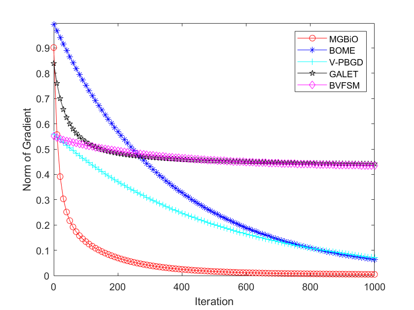
(a)

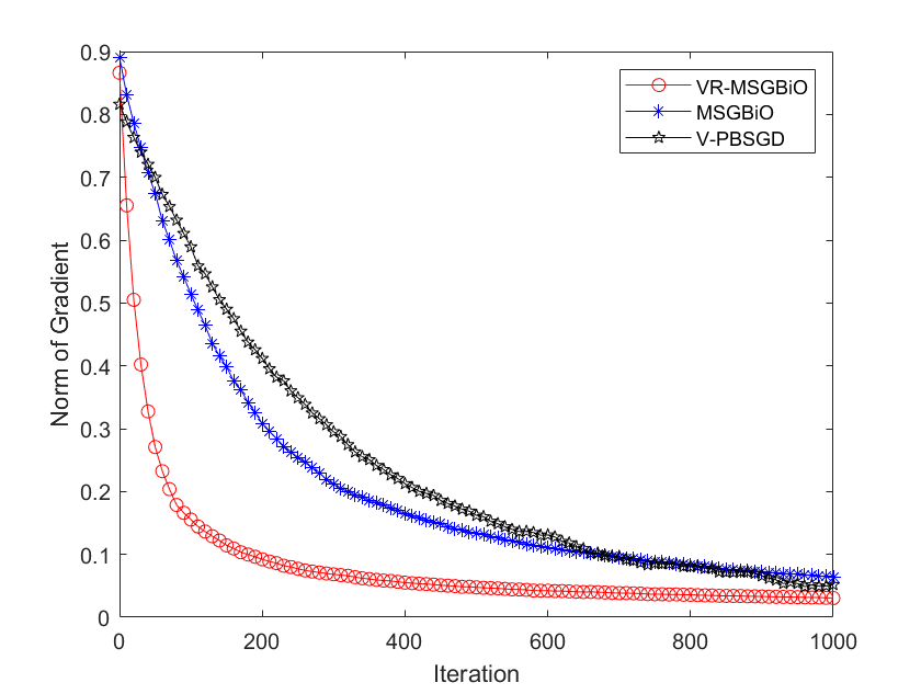
(b)

Figure 1: Norm of gradient against number of iteration: Left: deterministic algorithms, Right: stochastic algorithms.

5 Numerical Experiments

In the section, we conduct numerical experiments on bilevel PL game and hyper-representation learning to demonstrate the efficiency of our algorithms. In the experiments, we compare our algorithms with the baselines in the above Table 1. Meanwhile, we also add two baselines: BVFSM (Liu et al., 2021a) and GALET (Xiao et al., 2023).

(a)

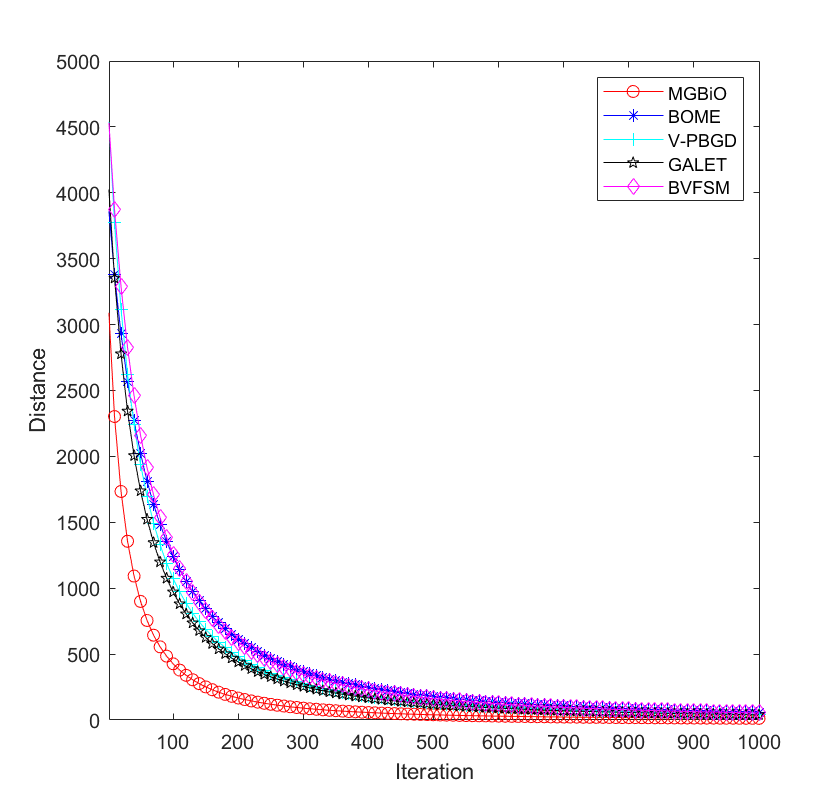
(b)

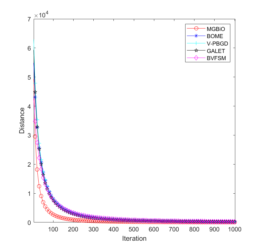
(c)

Figure 2: The ratio of distance $\|UU^{T}-H^{*}\|^{2}_{F}/\|H^{*}\|^{2}_{F}$ of deterministic algorithms under the case of $d=50$ (Left), $d=100$ (Middle) and $d=200$ (Right).

(a)

(b)

(c)

Figure 3: The loss of the deterministic algorithms under the case of $d=50$ (Left), $d=100$ (Middle) and $d=200$ (Right).

5.1 Bilevel Polyak-Łojasiewicz Game

In the subsection, we consider the following bilevel Polyak-Łojasiewicz Game:

$$\min_{x\in\mathbb{R}^{d}}\ \frac{1}{2}x^{T}Px+x^{T}R^{1}y,$$ (33)

$$\mbox{s.t.}\ \min_{y\in\mathbb{R}^{d}}\frac{1}{2}y^{T}Qy+x^{T}R^{2}y,$$

where $P=\frac{1}{n}\sum_{i=1}^{n}p_{i}(p_{i})^{T}$, $Q=\frac{1}{n}\sum_{i=1}^{n}q_{i}(q_{i})^{T}$, $R^{1}=\frac{1}{n}\sum_{i=1}^{n}0.01r^{1}_{i}(r^{1}_{i})^{T}$ and $R^{2}=\frac{1}{n}\sum_{i=1}^{n}0.01r^{2}_{i}(r^{2}_{i})^{T}$. Here the samples $\{p_{i}\}_{i=1}^{n}$, $\{q_{i}\}_{i=1}^{n}$, $\{r^{1}_{i}\}_{i=1}^{n}$ and $\{r^{2}_{i}\}_{i=1}^{n}$ are independently drawn from Gaussian distributions $\mathcal{N}(0,\Sigma_{P})$, $\mathcal{N}(0,\Sigma_{Q})$, $\mathcal{N}(0,\Sigma_{R^{1}})$ and $\mathcal{N}(0,\Sigma_{R^{2}})$, respectively. Meanwhile, we set $\Sigma_{P}=U^{1}D^{1}(U^{1})^{T}$, where $U^{1}\in\mathbb{R}^{d\times l}\ (l<d)$ is column orthogonal, and $D^{1}\in\mathbb{R}^{l\times l}$ is diagonal and its diagonal elements are distributed uniformly in the interval $[\mu,L]$ with $0<\mu<L$. Let $\Sigma_{Q}=U^{2}D^{2}(U^{2})^{T}$, where $U^{2}\in\mathbb{R}^{d\times l}$ is column orthogonal, and $D^{2}\in\mathbb{R}^{l\times l}$ is diagonal and its diagonal elements are distributed uniformly in the interval $[\mu,L]$ with $0<\mu<L$. We also set $\Sigma_{R^{1}}=0.001V^{1}(V^{1})^{T}$ and $\Sigma_{R^{2}}=0.001V^{2}(V^{2})^{T}$, where each element of $V^{1},V^{2}\in\mathbb{R}^{d\times d}$ is independently sampled from normal distribution $\mathcal{N}(0,1)$. Since the covariance matrices $\Sigma_{P}$ and $\Sigma_{Q}$ are rank-deficient, it is ensured that both $P$ and $Q$ are singular. Hence the lower-level and upper-level objective functions may be not convex, while they satisfy the PL condition. In this experiment, we set $d=50$, $l=48$ and $n=2500$. For fair comparison, we set the basic learning rate as $0.01$ for all algorithms. In the stochastic algorithms, we set mini-batch size as 10. From Figure 1, our deterministic MGBiO algorithm outperforms the baselines in Table 1. Meanwhile, our stochastic VR-MSGBiO algorithm outperforms the other algorithms.

(a)

(b)

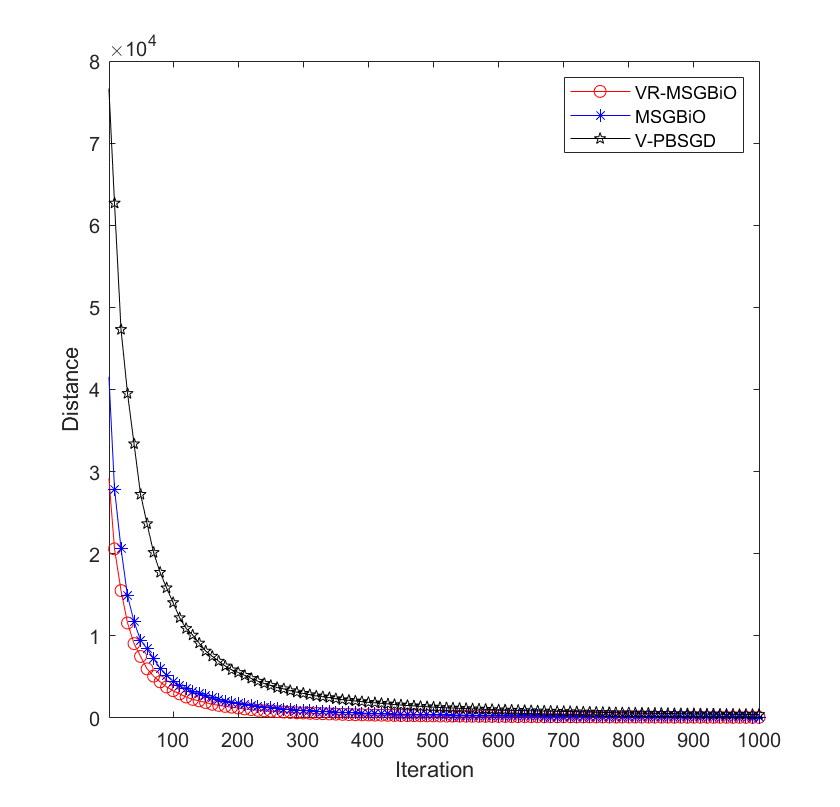
(c)

Figure 4: The ratio of distance $\|UU^{T}-H^{*}\|^{2}_{F}/\|H^{*}\|^{2}_{F}$ of the stochastic algorithms under the case of $d=50$ (Left), $d=100$ (Middle) and $d=200$ (Right).

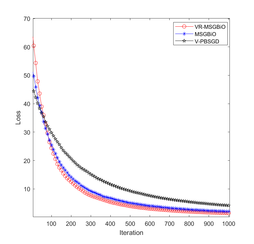
(a)

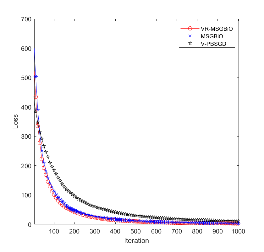
(b)

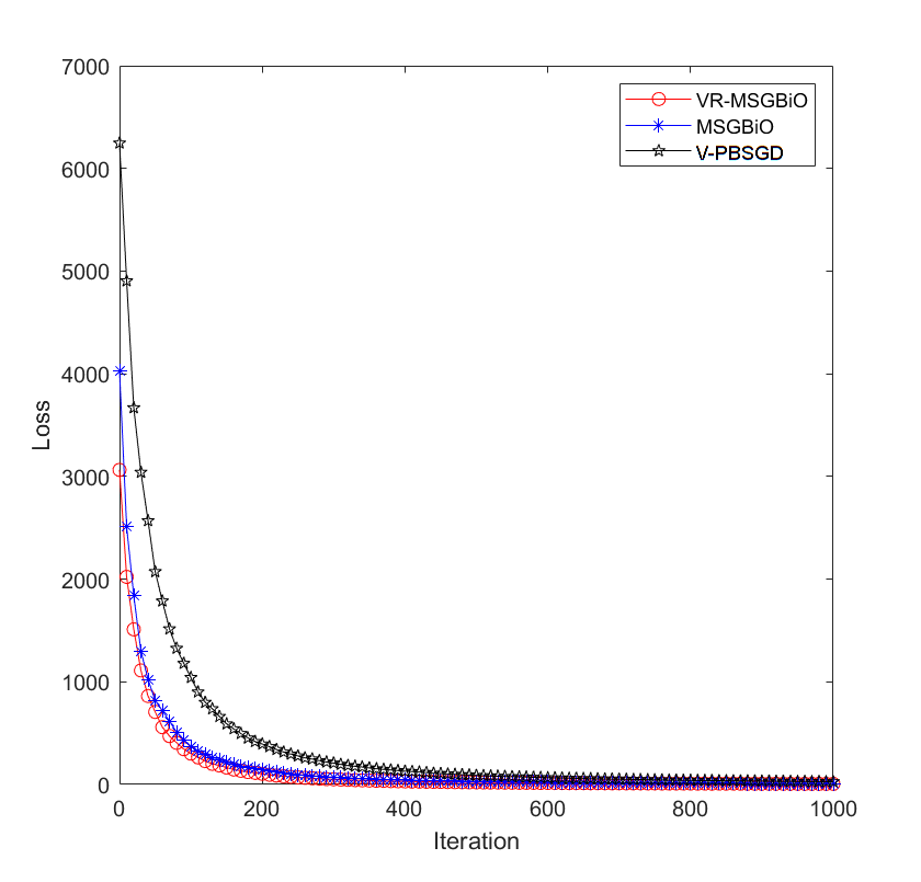
(c)

Figure 5: The loss of the stochastic algorithms under the case of $d=50$ (Left), $d=100$ (Middle) and $d=200$ (Right).

5.2 Hyper-Representation Learning

In the subsection, we conduct the hyper-representation learning task to verify the efficiency of our methods. Learning hyper-representation is one of key points of meta learning, which extract better feature representations to be applied to many different tasks. Here we specifically consider the hyper-representation learning in matrix sensing task. Given $n$ sensing matrices $\{C_{i}\in\mathbb{R}^{d\times d}\}_{i=1}^{n}$ with $n$ observations $e_{i}=\langle C_{i},H^{*}\rangle=\mbox{trace}(C_{i}^{T}H^{*})$, where $H^{*}=U^{*}(U^{*})^{T}$ is a low-rank symmetric matrix with $U^{*}\in\mathbb{R}^{d\times r}$. The goal of matrix sensing task is to find the matrix $U^{*}$, which can be represented the following problem:

$$\min_{U\in\mathbb{R}^{d\times r}}\frac{1}{n}\sum_{i=1}^{n}\ell_{i}(U)=\frac{1}{2}\big{(}\langle C_{i},UU^{T}\rangle-e_{i}\big{)}^{2}.$$ (34)

Then we consider the hyper-representation learning in matrix sensing task, which be rewritten the following bilevel optimization problem:

$$\min_{x\in\mathbb{R}^{d\times r-1}}\frac{1}{|D_{v}|}\sum_{i\in D_{v}}\ell_{i}(x,y^{*}(x)),$$ (35)

$$\mbox{s.t.}\ y^{*}(x)\in\arg\min_{y\in\mathbb{R}^{d}}\frac{1}{|D_{t}|}\sum_{i\in D_{t}}\ell_{i}(x,y),$$

where $U=[y;x]\in\mathbb{R}^{d\times r}$ is a concatenation of $x$ and $y$. Here we define variable $x$ to be the first $r-1$ columns of $U$ and variable $y$ to be the last column. Meanwhile, $D_{t}$ denotes the training dataset, and $D_{v}$ denotes the validation dataset. The ground truth low-rank matrix $H^{*}$ is generated by $H^{*}=U^{*}(U^{*})^{T}$, where each entry of $U^{*}$ is drawn from normal distribution $\mathbb{N}(0,\frac{1}{d})$ independently. We randomly generate $n=20d$ samples of sensing matrices $\{C_{i}\}_{i=1}^{n}$ from standard normal distribution, and then compute the corresponding no-noise labels $e_{i}=\langle C_{i},H^{*}\rangle$. We split all samples into two dataset: a train dataset $D_{t}$ with 40% data and a validation dataset $D_{v}$ with 60% data.

In the experiment, for fair comparison, we set the basic learning rate as $0.008$ for all algorithms. In the stochastic algorithms, we set mini-batch size as 10. Let $\ell(U)=\frac{1}{2n}\sum_{i=1}^{n}\big{(}\langle C_{i},UU^{T}\rangle-e_{i}\big{)}^{2}$ denote the loss. Figures 2-3 show that our deterministic MGBiO algorithm outperforms the baselines in Table 1. Figures 4-5 show that our stochastic VR-MSGBiO algorithm has a better performance than the other algorithms.

6 Conclusions

In the paper, we studied a class of non-convex bilevel optimization problems, where both upper-level and lower-level subproblems are nonconvex, and the lower-level subproblem satisfies PL condition. To solve these deterministic bilevel problems, we proposed an efficient momentum-based gradient bilevel (MGBiO) method, which reaches a lower gradient complexity of $O(\epsilon^{-2})$ in finding an $\epsilon$-stationary solution. Meanwhile, to solve these stochastic bilevel problems, we presented a class of efficient momentum-based stochastic gradient bilevel methods (i.e., MSGBiO, VR-MSGBiO). In particular, our VR-MSGBiO obtains an near-optimal gradient complexity $\tilde{O}(\epsilon^{-3})$ in finding an $\epsilon$-stationary solution. Experimental results on bilevel PL game and hyper-representation learning demonstrate the efficiency of our algorithms.

Appendix A Appendix

In this section, we provide the detailed convergence analysis of our algorithms. We first review some useful lemmas.

Lemma 6.

(Nesterov [2018]) Assume that $f(x)$ is a differentiable convex function and $\mathcal{X}$ is a convex set. $x^{*}\in\mathcal{X}$ is the solution of the constrained problem $\min_{x\in\mathcal{X}}f(x)$, if

$$\langle\nabla f(x^{*}),x-x^{*}\rangle\geq 0,\ \forall x\in\mathcal{X}.$$ (36)

Lemma 7.

(Karimi et al. [2016]) The function $f(x):\mathbb{R}^{d}\rightarrow\mathbb{R}$ is $L$-smooth and satisfies PL condition with constant $\mu$, then it also satisfies error bound (EB) condition with $\mu$, i.e., for all $x\in\mathbb{R}^{d}$

$$\|\nabla f(x)\|\geq\mu\|x^{*}-x\|,$$ (37)

where $x^{*}\in\arg\min_{x}f(x)$. It also satisfies quadratic growth (QG) condition with $\mu$, i.e.,

$$f(x)-\min_{x}f(x)\geq\frac{\mu}{2}\|x^{*}-x\|^{2}.$$ (38)

A.1 Convergence Analysis of MGBiO

In this subsection, we detail the convergence analysis of our MGBiO algorithm. We give some useful lemmas.

Lemma 8.

(Restatement of Lemma 1) Under the above Assumption 2, we have, for any $x\in\mathbb{R}^{d}$,

$$\nabla F(x)=\nabla_{x}f(x,y^{*}(x))-\nabla^{2}_{xy}g(x,y^{*}(x))\Big{[}\nabla^{2}_{yy}g(x,y^{*}(x))\Big{]}^{-1}\nabla_{y}f(x,y^{*}(x)).$$

Proof.

Since $F(x)=f(x,y^{*}(x))$, we have

$$\nabla F(x)=\nabla_{x}f(x,y^{*}(x))+\nabla y^{*}(x)\nabla_{y}f(x,y^{*}(x)).$$ (39)

Meanwhile, according to the optimal condition of the Lower-Level problem in Problem (1), we have

$$\nabla_{y}g(x,y^{*}(x))=0,$$ (40)

then further differentiating the above equality (40) on the variable $x$, we can obtain

$$\nabla_{x}\nabla_{y}g(x,y^{*}(x))+\nabla y^{*}(x)\nabla_{y}\nabla_{y}g(x,y^{*}(x))=0.$$ (41)

According to Assumption 1, the matrix $\nabla_{y}\nabla_{y}g(x,y^{*}(x))$ is reversible. Thus, we have

$$\nabla y^{*}(x)=-\nabla_{x}\nabla_{y}g(x,y^{*}(x))\big{(}\nabla_{y}\nabla_{y}g(x,y^{*}(x))\big{)}^{-1}.$$ (42)

Then we have

$$\nabla F(x) =\nabla_{x}f(x,y^{*}(x))-\nabla_{x}\nabla_{y}g(x,y^{*}(x))\big{(}\nabla_{y}\nabla_{y}g(x,y^{*}(x))\big{)}^{-1}\nabla_{y}f(x,y^{*}(x))$$

$$=\nabla_{x}f(x,y^{*}(x))-\nabla^{2}_{xy}g(x,y^{*}(x))\Big{[}\nabla^{2}_{yy}g(x,y^{*}(x))\Big{]}^{-1}\nabla_{y}f(x,y^{*}(x)).$$ (43)

∎

Lemma 9.

(Restatement of Lemma 2) Under the above Assumptions (1-3), the functions (or mappings) $F(x)=f(x,y^{*}(x))$, $G(x)=g(x,y^{*}(x))$ and $y^{*}(x)\in\arg\min_{y\in\mathbb{R}^{p}}g(x,y)$ satisfy, for all $x_{1},x_{2}\in\mathbb{R}^{d}$,

$$\|y^{*}(x_{1})-y^{*}(x_{2})\|\leq\kappa\|x_{1}-x_{2}\|,\quad\|\nabla y^{*}(x_{1})-\nabla y^{*}(x_{2})\|\leq L_{y}\|x_{1}-x_{2}\|$$

$$\|\nabla F(x_{1})-\nabla F(x_{2})\|\leq L_{F}\|x_{1}-x_{2}\|,\quad\|\nabla G(x_{1})-\nabla G(x_{2})\|\leq L_{G}\|x_{1}-x_{2}\|$$

where $\kappa=C_{gxy}/\mu$, $L_{y}=\big{(}\frac{C_{gxy}L_{gyy}}{\mu^{2}}+\frac{L_{gxy}}{\mu}\big{)}(1+\frac{C_{gxy}}{\mu})$, $L_{F}=\Big{(}L_{f}+L_{f}\kappa+C_{fy}\big{(}\frac{C_{gxy}L_{gyy}}{\mu^{2}}+\frac{L_{gxy}}{\mu}\big{)}\Big{)}(1+\kappa)$ and $L_{G}=\Big{(}L_{g}+L_{g}\kappa+C_{gy}\big{(}\frac{C_{gxy}L_{gyy}}{\mu^{2}}+\frac{L_{gxy}}{\mu}\big{)}\Big{)}(1+\kappa)$.

Proof.

From the above lemma 8, we have

$$\nabla y^{*}(x)=-\nabla^{2}_{xy}g(x,y^{*}(x))\Big{(}\nabla^{2}_{yy}g(x,y^{*}(x))\Big{)}^{-1}.$$ (44)

According to the above Assumptions 2 and 3, we have for any $x\in\mathbb{R}^{d}$,

$$\|\nabla y^{*}(x)\| =\|-\nabla^{2}_{xy}g(x,y^{*}(x))\Big{(}\nabla^{2}_{yy}g(x,y^{*}(x))\Big{)}^{-1}\|$$

$$\leq\|\nabla^{2}_{xy}g(x,y^{*}(x))\|\|\big{(}\nabla^{2}_{yy}g(x,y^{*}(x))\big{)}^{-1}\|\leq\frac{C_{gxy}}{\mu}.$$ (45)

By using the Mean Value Theorem, we have for any $x_{1},x_{2}\in\mathbb{R}^{d}$

$$\|y^{*}(x_{1})-y^{*}(x_{1})\|=\|\nabla y^{*}(z)(x_{1}-x_{2})\|\leq\frac{C_{gxy}}{\mu}\|x_{1}-x_{2}\|,$$ (46)

where $z\in(x_{1},x_{2})$.

For any $x_{1},x_{2}\in\mathbb{R}^{d}$, we have

$$\|\nabla y^{*}(x_{1})-\nabla y^{*}(x_{2})\|$$

$$=\big{\|}\nabla^{2}_{xy}g(x_{1},y^{*}(x_{1}))\Big{(}\nabla^{2}_{yy}g(x_{1},y^{*}(x_{1}))\Big{)}^{-1}-\nabla^{2}_{xy}g(x_{2},y^{*}(x_{2}))\Big{(}\nabla^{2}_{yy}g(x_{2},y^{*}(x_{2}))\Big{)}^{-1}\big{\|}$$

$$\leq\|\nabla^{2}_{xy}g(x_{1},y^{*}(x_{1}))\Big{(}\nabla^{2}_{yy}g(x_{1},y^{*}(x_{1}))\Big{)}^{-1}-\nabla^{2}_{xy}g(x_{1},y^{*}(x_{1}))\Big{(}\nabla^{2}_{yy}g(x_{2},y^{*}(x_{2}))\Big{)}^{-1}\|$$

$$\quad+\|\nabla^{2}_{xy}g(x_{1},y^{*}(x_{1}))\Big{(}\nabla^{2}_{yy}g(x_{2},y^{*}(x_{2}))\Big{)}^{-1}-\nabla^{2}_{xy}g(x_{2},y^{*}(x_{2}))\Big{(}\nabla^{2}_{yy}g(x_{2},y^{*}(x_{2}))\Big{)}^{-1}\|$$

$$\leq C_{gxy}\sum_{m=1}\|\Big{(}\nabla^{2}_{yy}g(x_{1},y^{*}(x_{1}))\Big{)}^{-1}-\Big{(}\nabla^{2}_{yy}g(x_{2},y^{*}(x_{2}))\Big{)}^{-1}\|$$

$$\quad+\frac{1}{\mu}\sum_{m=1}\|\nabla^{2}_{xy}g(x_{1},y^{*}(x_{1}))-\nabla^{2}_{xy}g(x_{2},y^{*}(x_{2}))\|$$

$$\leq C_{gxy}\sum_{m=1}\|\Big{(}\nabla^{2}_{yy}g(x_{2},y^{*}(x_{2}))\Big{)}^{-1}\Big{(}\nabla^{2}_{yy}g(x_{2},y^{*}(x_{2}))-\nabla^{2}_{yy}g(x_{1},y^{*}(x_{1}))\Big{)}$$

$$\quad\cdot\Big{(}\nabla^{2}_{yy}g(x_{1},y^{*}(x_{1}))\Big{)}^{-1}\|+\frac{1}{\mu}\sum_{m=1}\Big{(}L_{gxy}\|x_{1}-x_{2}\|+L_{gxy}\|y^{*}(x_{1})-y^{*}(x_{2})\|\Big{)}$$

$$\leq\frac{C_{gxy}}{\mu^{2}}\sum_{m=1}\|\big{(}\nabla^{2}_{yy}g(x_{2},y^{*}(x_{2}))-\nabla^{2}_{yy}g(x_{1},y^{*}(x_{1}))\big{)}\|+\frac{1}{\mu}\sum_{m=1}\Big{(}L_{gxy}\|x_{1}-x_{2}\|+L_{gxy}\|y^{*}(x_{1})-y^{*}(x_{2})\|\Big{)}$$

$$\leq\frac{C_{gxy}}{\mu^{2}}\sum_{m=1}\big{(}L_{gyy}\|x_{1}-x_{2}\|+L_{gyy}\|y^{*}(x_{1})-y^{*}(x_{2})\|\big{)}+\frac{1}{\mu}\sum_{m=1}\Big{(}L_{gxy}\|x_{1}-x_{2}\|+L_{gxy}\|y^{*}(x_{1})-y^{*}(x_{2})\|\Big{)}$$

$$\leq\big{(}\frac{C_{gxy}L_{gyy}}{\mu^{2}}+\frac{L_{gxy}}{\mu}\big{)}(1+\frac{C_{gxy}}{\mu})\|x_{1}-x_{2}\|,$$ (47)

where the last inequality holds by the above inequality (46).

From the above lemma 1, we have

$$\nabla F(x)=\nabla_{x}f(x,y^{*}(x))+\nabla y^{*}(x)^{T}\nabla_{y}f(x,y^{*}(x)),$$ (48)

then for any $x_{1},x_{2}\in\mathbb{R}^{d}$, we have

$$\|\nabla F(x_{1})-\nabla F(x_{2})\|$$

$$=\|\nabla_{x}f(x_{1},y^{*}(x_{1}))+\nabla y^{*}(x_{1})^{T}\Big{(}\nabla_{y}f(x_{1},y^{*}(x_{1}))\Big{)}$$

$$\qquad-\nabla_{x}f(x_{1},y^{*}(x_{2}))-\nabla y^{*}(x_{2})^{T}\Big{(}\nabla_{y}f(x_{2},y^{*}(x_{2}))\Big{)}\|$$

$$\leq L_{f}\big{(}\|x_{1}-x_{2}\|+\|y^{*}(x_{1})-y^{*}(x_{2})\|\big{)}+\|\nabla y^{*}(x_{1})^{T}\Big{(}\nabla_{y}f(x_{1},y^{*}(x_{1}))\Big{)}$$

$$\quad-\nabla y^{*}(x_{2})^{T}\Big{(}\nabla_{y}f(x_{1},y^{*}(x_{1}))\Big{)}+\nabla y^{*}(x_{2})^{T}\Big{(}\nabla_{y}f(x_{1},y^{*}(x_{1}))\Big{)}$$

$$\quad-\nabla y^{*}(x_{2})^{T}\Big{(}\nabla_{y}f(x_{2},y^{*}(x_{2}))\Big{)}\|$$

$$\leq L_{f}\big{(}\|x_{1}-x_{2}\|+\|y^{*}(x_{1})-y^{*}(x_{2})\|\big{)}+C_{fy}\|\nabla y^{*}(x_{1})-\nabla y^{*}(x_{2})\|$$

$$\quad+\frac{C_{gxy}}{\mu}\|\nabla_{y}f(x_{1},y^{*}(x_{1}))-\nabla_{y}f(x_{2},y^{*}(x_{2}))\|$$

$$\leq L_{f}(1+\frac{C_{gxy}}{\mu})\|x_{1}-x_{2}\|+C_{fy}\|\nabla y^{*}(x_{1})-\nabla y^{*}(x_{2})\|+\frac{C_{gxy}L_{f}}{\mu}(1+\frac{C_{gxy}}{\mu})\|x_{1}-x_{2}\|$$

$$\leq\Big{(}L_{f}+\frac{C_{gxy}L_{f}}{\mu}+C_{fy}\big{(}\frac{C_{gxy}L_{gyy}}{\mu^{2}}+\frac{L_{gxy}}{\mu}\big{)}\Big{)}(1+\frac{C_{gxy}}{\mu})\|x_{1}-x_{2}\|,$$ (49)

where the last inequality holds by (A.1).

Since $\nabla G(x)=\nabla_{x}g(x,y^{*}(x))+\nabla y^{*}(x)^{T}\nabla_{y}g(x,y^{*}(x))$, we have for any $x_{1},x_{2}\in\mathbb{R}^{d}$

$$\|\nabla G(x_{1})-\nabla G(x_{2})\|$$

$$=\|\nabla_{x}g(x_{1},y^{*}(x_{1}))+\nabla y^{*}(x_{1})^{T}\Big{(}\nabla_{y}g(x_{1},y^{*}(x_{1}))\Big{)}$$

$$\qquad-\nabla_{x}g(x_{1},y^{*}(x_{2}))-\nabla y^{*}(x_{2})^{T}\Big{(}\nabla_{y}g(x_{2},y^{*}(x_{2}))\Big{)}\|$$

$$\leq L_{g}\big{(}\|x_{1}-x_{2}\|+\|y^{*}(x_{1})-y^{*}(x_{2})\|\big{)}+\|\nabla y^{*}(x_{1})^{T}\Big{(}\nabla_{y}g(x_{1},y^{*}(x_{1}))\Big{)}$$

$$\quad-\nabla y^{*}(x_{2})^{T}\Big{(}\nabla_{y}g(x_{1},y^{*}(x_{1}))\Big{)}+\nabla y^{*}(x_{2})^{T}\Big{(}\nabla_{y}g(x_{1},y^{*}(x_{1}))\Big{)}$$

$$\quad-\nabla y^{*}(x_{2})^{T}\Big{(}\nabla_{y}g(x_{2},y^{*}(x_{2}))\Big{)}\|$$

$$\leq L_{g}\big{(}\|x_{1}-x_{2}\|+\|y^{*}(x_{1})-y^{*}(x_{2})\|\big{)}+C_{gy}\|\nabla y^{*}(x_{1})-\nabla y^{*}(x_{2})\|$$

$$\quad+\frac{C_{gxy}}{\mu}\|\nabla_{y}g(x_{1},y^{*}(x_{1}))-\nabla_{y}g(x_{2},y^{*}(x_{2}))\|$$

$$\leq L_{g}(1+\frac{C_{gxy}}{\mu})\|x_{1}-x_{2}\|+C_{gy}\|\nabla y^{*}(x_{1})-\nabla y^{*}(x_{2})\|+\frac{C_{gxy}L_{g}}{\mu}(1+\frac{C_{gxy}}{\mu})\|x_{1}-x_{2}\|$$

$$\leq\Big{(}L_{g}+\frac{C_{gxy}L_{g}}{\mu}+C_{gy}\big{(}\frac{C_{gxy}L_{gyy}}{\mu^{2}}+\frac{L_{gxy}}{\mu}\big{)}\Big{)}(1+\frac{C_{gxy}}{\mu})\|x_{1}-x_{2}\|.$$ (50)

∎

Lemma 10.

(Restatement of Lemma 3) Let $\hat{\nabla}f(x,y)=\nabla_{x}f(x,y)-\hat{\Pi}_{C_{gxy}}\big{[}\nabla^{2}_{xy}g(x,y)\big{]}\big{(}\mathcal{S}_{[\mu,L_{g}]}\big{[}\nabla^{2}_{yy}g(x,y)\big{]}\big{)}^{-1}\Pi_{C_{fy}}\big{[}\nabla_{y}f(x,y)\big{]}$ and $\nabla F(x)=\nabla f(x,y^{*}(x))$, we have

$$\|\hat{\nabla}f(x,y)-\nabla F(x)\|^{2}\leq\hat{L}^{2}\|y^{*}(x)-y\|^{2}\leq\frac{2\hat{L}^{2}}{\mu}\big{(}g(x,y)-\min_{y}g(x,y)\big{)},$$ (51)

where $\hat{L}^{2}=4\big{(}L^{2}_{f}+\frac{L^{2}_{gxy}C^{2}_{fy}}{\mu^{2}}+\frac{L^{2}_{gyy}C^{2}_{gxy}C^{2}_{fy}}{\mu^{4}}+\frac{L^{2}_{f}C^{2}_{gxy}}{\mu^{2}}\big{)}$.

Proof.

Since $\nabla F(x)=\nabla f(x,y^{*}(x))$, we have

$$\|\nabla f(x,y^{*}(x))-\hat{\nabla}f(x,y)\|^{2}$$

$$=\|\nabla_{x}f(x,y^{*}(x))-\nabla^{2}_{xy}g(x,y^{*}(x))\big{(}\nabla^{2}_{yy}g(x,y^{*}(x))\big{)}^{-1}\nabla_{y}f(x,y^{*}(x))$$

$$\quad-\nabla_{x}f(x,y)+\hat{\Pi}_{C_{gxy}}\big{[}\nabla^{2}_{xy}g(x,y)\big{]}\big{(}\mathcal{S}_{[\mu,L_{g}]}\big{[}\nabla^{2}_{yy}g(x,y)\big{]}\big{)}^{-1}\Pi_{C_{fy}}\big{[}\nabla_{y}f(x,y)\big{]}\|^{2}$$

$$=\|\nabla_{x}f(x,y^{*}(x))-\nabla_{x}f(x,y)-\nabla^{2}_{xy}g(x,y^{*}(x))\big{(}\nabla^{2}_{yy}g(x,y^{*}(x))\big{)}^{-1}\nabla_{y}f(x,y^{*}(x))$$

$$\quad+\hat{\Pi}_{C_{gxy}}\big{[}\nabla^{2}_{xy}g(x,y)\big{]}\big{(}\nabla^{2}_{yy}g(x,y^{*}(x))\big{)}^{-1}\nabla_{y}f(x,y^{*}(x))-\hat{\Pi}_{C_{gxy}}\big{[}\nabla^{2}_{xy}g(x,y)\big{]}\big{(}\nabla^{2}_{yy}g(x,y^{*}(x))\big{)}^{-1}\nabla_{y}f(x,y^{*}(x))$$

$$\quad+\hat{\Pi}_{C_{gxy}}\big{[}\nabla^{2}_{xy}g(x,y)\big{]}\big{(}\mathcal{S}_{[\mu,L_{g}]}\big{[}\nabla^{2}_{yy}g(x,y)\big{]}\big{)}^{-1}\nabla_{y}f(x,y^{*}(x))-\hat{\Pi}_{C_{gxy}}\big{[}\nabla^{2}_{xy}g(x,y)\big{]}\big{(}\mathcal{S}_{[\mu,L_{g}]}\big{[}\nabla^{2}_{yy}g(x,y)\big{]}\big{)}^{-1}\nabla_{y}f(x,y^{*}(x))$$

$$\quad+\hat{\Pi}_{C_{gxy}}\big{[}\nabla^{2}_{xy}g(x,y)\big{]}\big{(}\mathcal{S}_{[\mu,L_{g}]}\big{[}\nabla^{2}_{yy}g(x,y)\big{]}\big{)}^{-1}\Pi_{C_{fy}}\big{[}\nabla_{y}f(x,y)\big{]}\|^{2}$$

$$\leq 4\|\nabla_{x}f(x,y^{*}(x))-\nabla_{x}f(x,y)\|^{2}+\frac{4C^{2}_{fy}}{\mu^{2}}\|\nabla^{2}_{xy}g(x,y^{*}(x))-\hat{\Pi}_{C_{gxy}}\big{[}\nabla^{2}_{xy}g(x,y)\big{]}\|^{2}$$

$$\quad+\frac{4C^{2}_{gxy}C^{2}_{fy}}{\mu^{4}}\|\nabla^{2}_{yy}g(x,y^{*}(x))-\mathcal{S}_{[\mu,L_{g}]}\big{[}\nabla^{2}_{yy}g(x,y)\big{]}\|^{2}+\frac{4C^{2}_{gxy}}{\mu^{2}}\|\nabla_{y}f(x,y^{*}(x))-\Pi_{C_{fy}}\big{[}\nabla_{y}f(x,y)\big{]}\|^{2}$$

$$\mathop{=}^{(i)}4\|\nabla_{x}f(x,y^{*}(x))-\nabla_{x}f(x,y)\|^{2}+\frac{4C^{2}_{fy}}{\mu^{2}}\|\hat{\Pi}_{C_{gxy}}\big{[}\nabla^{2}_{xy}g(x,y^{*}(x))\big{]}-\hat{\Pi}_{C_{gxy}}\big{[}\nabla^{2}_{xy}g(x,y)\big{]}\|^{2}$$

$$\quad+\frac{4C^{2}_{gxy}C^{2}_{fy}}{\mu^{4}}\|\mathcal{S}_{[\mu,L_{g}]}\big{[}\nabla^{2}_{yy}g(x,y^{*}(x))\big{]}-\mathcal{S}_{[\mu,L_{g}]}\big{[}\nabla^{2}_{yy}g(x,y)\big{]}\|^{2}+\frac{4C^{2}_{gxy}}{\mu^{2}}\|\Pi_{C_{fy}}\big{[}\nabla_{y}f(x,y^{*}(x))\big{]}-\Pi_{C_{fy}}\big{[}\nabla_{y}f(x,y)\big{]}\|^{2}$$

$$\leq 4\|\nabla_{x}f(x,y^{*}(x))-\nabla_{x}f(x,y)\|^{2}+\frac{4C^{2}_{fy}}{\mu^{2}}\|\nabla^{2}_{xy}g(x,y^{*}(x))-\nabla^{2}_{xy}g(x,y)\|^{2}$$

$$\quad+\frac{4C^{2}_{gxy}C^{2}_{fy}}{\mu^{4}}\|\nabla^{2}_{yy}g(x,y^{*}(x))-\nabla^{2}_{yy}g(x,y)\|^{2}+\frac{4C^{2}_{gxy}}{\mu^{2}}\|\nabla_{y}f(x,y^{*}(x))-\nabla_{y}f(x,y)\|^{2}$$

$$\leq 4\big{(}L^{2}_{f}+\frac{L^{2}_{gxy}C^{2}_{fy}}{\mu^{2}}+\frac{L^{2}_{gyy}C^{2}_{gxy}C^{2}_{fy}}{\mu^{4}}+\frac{L^{2}_{f}C^{2}_{gxy}}{\mu^{2}}\big{)}\|y^{*}(x)-y\|^{2}$$

$$=\hat{L}^{2}\|y^{*}(x)-y\|^{2}\leq\frac{2\hat{L}^{2}}{\mu}\big{(}g(x,y)-\min_{y}g(x,y)\big{)},$$ (52)

where the above equality (i) due to Assumption 2, i.e., $\mathcal{S}_{[\mu,L_{g}]}\big{[}\nabla^{2}_{yy}g(x,y^{*}(x))\big{]}=\nabla^{2}_{yy}g(x,y^{*}(x))$ and Assumption 3, i.e., $\hat{\Pi}_{C_{gxy}}\big{[}\nabla^{2}_{xy}g(x,y^{*}(x))\big{]}=\nabla^{2}_{xy}g(x,y^{*}(x))$, $\Pi_{C_{fy}}\big{[}\nabla_{y}f(x,y^{*}(x))\big{]}=\nabla_{y}f(x,y^{*}(x))$, and the second last inequality is due to Assumptions 2-4; the last inequality holds by Lemma 7.

∎

Lemma 11.

(Restatement of Lemma 4) Suppose the sequence $\{x_{t},y_{t}\}_{t=1}^{T}$ be generated from Algorithm 1 or 2 or 3. Under the above Assumptions 1-2, given $\gamma\leq\frac{\lambda\mu}{8L_{G}}$ and $0<\lambda\leq\frac{1}{2L_{g}\eta_{t}}$ for all $t\geq 1$, we have

$$g(x_{t+1},y_{t+1})-G(x_{t+1}) \leq(1-\frac{\eta_{t}\lambda\mu}{2})\big{(}g(x_{t},y_{t})-G(x_{t})\big{)}+\frac{\eta_{t}}{8\gamma}\|\tilde{x}_{t+1}-x_{t}\|^{2}-\frac{\eta_{t}}{4\lambda}\|\tilde{y}_{t+1}-y_{t}\|^{2}$$

$$\quad+\eta_{t}\lambda\|\nabla_{y}g(x_{t},y_{t})-v_{t}\|^{2},$$ (53)

where $G(x_{t})=g(x_{t},y^{*}(x_{t}))$ with $y^{*}(x_{t})\in\arg\min_{y}g(x_{t},y)$ for all $t\geq 1$.

Proof.

By using Assumption 3, i.e., $L_{g}$-smoothness of $g(x,\cdot)$, such that

$$g(x_{t+1},y_{t+1})\leq g(x_{t+1},y_{t})+\langle\nabla_{y}g(x_{t+1},y_{t}),y_{t+1}-y_{t}\rangle+\frac{L_{g}}{2}\|y_{t+1}-y_{t}\|^{2},$$ (54)

then we have

$$g(x_{t+1},y_{t+1})\leq g(x_{t+1},y_{t})+\eta_{t}\langle\nabla_{y}g(x_{t+1},y_{t}),\tilde{y}_{t+1}-y_{t}\rangle+\frac{L_{g}\eta^{2}_{t}}{2}\|\tilde{y}_{t+1}-y_{t}\|^{2}.$$ (55)

Next, we bound the inner product in (55),

$$\eta_{t}\langle\nabla_{y}g(x_{t+1},y_{t}),\tilde{y}_{t+1}-y_{t}\rangle=-\eta_{t}\lambda\langle\nabla_{y}g(x_{t+1},y_{t}),v_{t}\rangle$$

$$=-\frac{\eta_{t}\lambda}{2}\Big{(}\|\nabla_{y}g(x_{t+1},y_{t})\|^{2}+\|v_{t}\|^{2}-\|\nabla_{y}g(x_{t+1},y_{t})-\nabla_{y}g(x_{t},y_{t})+\nabla_{y}g(x_{t},y_{t})-v_{t}\|^{2}\Big{)}$$

$$\leq-\frac{\eta_{t}\lambda}{2}\|\nabla_{y}g(x_{t+1},y_{t})\|^{2}-\frac{\eta_{t}}{2\lambda}\|\tilde{y}_{t+1}-y_{t}\|^{2}+\eta_{t}\lambda L^{2}_{g}\|x_{t+1}-x_{t}\|^{2}+\eta_{t}\lambda\|\nabla_{y}g(x_{t},y_{t})-v_{t}\|^{2}$$

$$\leq-\eta_{t}\lambda\mu\big{(}g(x_{t+1},y_{t})-G(x_{t+1})\big{)}-\frac{\eta_{t}}{2\lambda}\|\tilde{y}_{t+1}-y_{t}\|^{2}+\eta_{t}\lambda L^{2}_{g}\|x_{t+1}-x_{t}\|^{2}+\eta_{t}\lambda\|\nabla_{y}g(x_{t},y_{t})-v_{t}\|^{2},$$ (56)

where the last inequality is due to the quadratic growth condition of $\mu$-PL functions, i.e.,

$$\|\nabla_{y}g(x_{t+1},y_{t})\|^{2}\geq 2\mu\big{(}g(x_{t+1},y_{t})-\min_{y^{\prime}}g(x_{t+1},y^{\prime})\big{)}=2\mu\big{(}g(x_{t+1},y_{t})-G(x_{t+1})\big{)}.$$ (57)

Substituting (A.1) in (55), we have

$$g(x_{t+1},y_{t+1}) \leq g(x_{t+1},y_{t})-\eta_{t}\lambda\mu\big{(}g(x_{t+1},y_{t})-G(x_{t+1})\big{)}-\frac{\eta_{t}}{2\lambda}\|\tilde{y}_{t+1}-y_{t}\|^{2}+\eta_{t}\lambda L^{2}_{g}\|x_{t+1}-x_{t}\|^{2}$$

$$\quad+\eta_{t}\lambda\|\nabla_{y}g(x_{t},y_{t})-v_{t}\|^{2}+\frac{L_{g}\eta^{2}_{t}}{2}\|\tilde{y}_{t+1}-y_{t}\|^{2},$$ (58)

then rearranging the terms, we can obtain

$$g(x_{t+1},y_{t+1})-G(x_{t+1}) \leq(1-\eta_{t}\lambda\mu)\big{(}g(x_{t+1},y_{t})-G(x_{t+1})\big{)}-\frac{\eta_{t}}{2\lambda}\|\tilde{y}_{t+1}-y_{t}\|^{2}+\eta_{t}\lambda L^{2}_{g}\|x_{t+1}-x_{t}\|^{2}$$

$$\quad+\eta_{t}\lambda\|\nabla_{y}g(x_{t},y_{t})-v_{t}\|^{2}+\frac{L_{g}\eta^{2}_{t}}{2}\|\tilde{y}_{t+1}-y_{t}\|^{2}.$$ (59)

Next, using $L_{g}$-smoothness of function $f(\cdot,y_{t})$, such that

$$g(x_{t+1},y_{t})\leq g(x_{t},y_{t})+\langle\nabla_{x}g(x_{t},y_{t}),x_{t+1}-x_{t}\rangle+\frac{L_{g}}{2}\|x_{t+1}-x_{t}\|^{2},$$ (60)

then we have

$$g(x_{t+1},y_{t})-g(x_{t},y_{t})$$

$$\leq\langle\nabla_{x}g(x_{t},y_{t}),x_{t+1}-x_{t}\rangle+\frac{L_{g}}{2}\|x_{t+1}-x_{t}\|^{2}$$

$$=\eta_{t}\langle\nabla_{x}g(x_{t},y_{t})-\nabla G(x_{t}),\tilde{x}_{t+1}-x_{t}\rangle+\eta_{t}\langle\nabla G(x_{t}),\tilde{x}_{t+1}-x_{t}\rangle+\frac{L_{g}\eta^{2}_{t}}{2}\|\tilde{x}_{t+1}-x_{t}\|^{2}$$

$$\leq\frac{\eta_{t}}{8\gamma}\|\tilde{x}_{t+1}-x_{t}\|^{2}+2\eta_{t}\gamma\|\nabla_{x}g(x_{t},y_{t})-\nabla G(x_{t})\|^{2}+\eta_{t}\langle\nabla G(x_{t}),\tilde{x}_{t+1}-x_{t}\rangle+\frac{L_{g}\eta^{2}_{t}}{2}\|\tilde{x}_{t+1}-x_{t}\|^{2}$$

$$\leq\frac{\eta_{t}}{8\gamma}\|\tilde{x}_{t+1}-x_{t}\|^{2}+2L^{2}_{g}\eta_{t}\gamma\|y_{t}-y^{*}(x_{t})\|^{2}+G(x_{t+1})-G(x_{t})$$

$$\quad+\frac{\eta^{2}_{t}L_{G}}{2}\|\tilde{x}_{t+1}-x_{t}\|^{2}+\frac{\eta^{2}_{t}L_{g}}{2}\|\tilde{x}_{t+1}-x_{t}\|^{2}$$

$$\leq\frac{4L^{2}_{g}\eta_{t}\gamma}{\mu}\big{(}g(x_{t},y_{t})-G(x_{t})\big{)}+G(x_{t+1})-G(x_{t})+(\frac{\eta_{t}}{8\gamma}+\eta^{2}_{t}L_{G})\|\tilde{x}_{t+1}-x_{t}\|^{2},$$ (61)

where the second last inequality is due to $L_{G}$-smoothness of function $G(x)$, and the last inequality holds by Lemma 7 and $L_{g}\leq L_{G}$. Then we have

$$g(x_{t+1},y_{t})-G(x_{t+1}) =g(x_{t+1},y_{t})-g(x_{t},y_{t})+g(x_{t},y_{t})-G(x_{t})+G(x_{t})-G(x_{t+1})$$

$$\leq(1+\frac{4L^{2}_{g}\eta_{t}\gamma}{\mu})\big{(}g(x_{t},y_{t})-G(x_{t})\big{)}+(\frac{\eta_{t}}{8\gamma}+\eta^{2}_{t}L_{G})\|\tilde{x}_{t+1}-x_{t}\|^{2}.$$ (62)

Substituting (A.1) in (A.1), we get

$$g(x_{t+1},y_{t+1})-G(x_{t+1})$$

$$\leq(1-\eta_{t}\lambda\mu)(1+\frac{4L^{2}_{g}\eta_{t}\gamma}{\mu})\big{(}g(x_{t},y_{t})-G(x_{t})\big{)}+\eta_{t}(\frac{1}{8\gamma}+\eta_{t}L_{G})(1-\eta_{t}\lambda\mu)\|\tilde{x}_{t+1}-x_{t}\|^{2}$$

$$\quad-\frac{\eta_{t}}{2\lambda}\|\tilde{y}_{t+1}-y_{t}\|^{2}+\eta_{t}\lambda L^{2}_{g}\|x_{t+1}-x_{t}\|^{2}+\eta_{t}\lambda\|\nabla_{y}g(x_{t},y_{t})-v_{t}\|^{2}+\frac{L_{g}\eta^{2}_{t}}{2}\|\tilde{y}_{t+1}-y_{t}\|^{2}$$

$$=(1-\eta_{t}\lambda\mu)(1+\frac{4L^{2}_{g}\eta_{t}\gamma}{\mu})\big{(}g(x_{t},y_{t})-G(x_{t})\big{)}+\eta_{t}\big{(}\frac{1}{8\gamma}+\eta_{t}L_{G}-\frac{\eta_{t}\lambda\mu}{8\gamma}-\eta^{2}_{t}L_{G}\lambda\mu+\eta^{2}_{t}L^{2}_{g}\lambda\big{)}\|\tilde{x}_{t+1}-x_{t}\|^{2}$$

$$\quad-\frac{\eta_{t}}{2}\big{(}\frac{1}{\lambda}-L_{g}\eta_{t}\big{)}\|\tilde{y}_{t+1}-y_{t}\|^{2}+\eta_{t}\lambda\|\nabla_{y}g(x_{t},y_{t})-v_{t}\|^{2}$$

$$\leq(1-\frac{\eta_{t}\lambda\mu}{2})\big{(}g(x_{t},y_{t})-G(x_{t})\big{)}+\frac{\eta_{t}}{8\gamma}\|\tilde{x}_{t+1}-x_{t}\|^{2}-\frac{\eta_{t}}{4\lambda}\|\tilde{y}_{t+1}-y_{t}\|^{2}+\eta_{t}\lambda\|\nabla_{y}g(x_{t},y_{t})-v_{t}\|^{2},$$ (63)

where the last inequality holds by $\gamma\leq\frac{\lambda\mu}{8L_{G}}$, $L_{G}\geq L_{g}(1+\kappa)^{2}$ and $\lambda\leq\frac{1}{2L_{g}\eta_{t}}$ for all $t\geq 1$, i.e.,

$$\gamma\leq\frac{\lambda\mu}{8L_{G}}\Rightarrow\lambda\geq\frac{8L_{G}\gamma}{\mu}\geq\frac{8L_{g}}{\mu}(1+\kappa)^{2}\gamma\geq 8\kappa^{2}\gamma\Rightarrow\frac{\eta_{t}\lambda\mu}{2}\geq\frac{4L^{2}_{f}\eta_{t}\gamma}{\mu}$$

$$L_{G}\geq L_{g}(1+\kappa)^{2}\geq L_{g}(1+\kappa)\Rightarrow\eta^{2}_{t}L_{G}\lambda\mu\geq\eta^{2}_{t}L^{2}_{f}\lambda$$

$$\lambda\leq\frac{1}{2\eta_{t}L_{g}}\Rightarrow\frac{1}{2\lambda}\geq\eta_{t}L_{g},\ \forall t\geq 1.$$ (64)

∎

Theorem 5.

(Restatement of Theorem 1) Under the above Assumptions (1-5), in the Algorithm 1, let $\eta_{t}=\eta$ for all $t\geq 0$, $0<\gamma\leq\min\big{(}\frac{1}{2L_{F}\eta},\frac{\lambda\mu^{2}}{16\hat{L}^{2}}\big{)}$, $0<\lambda\leq\frac{1}{2L_{g}\eta}$. When $\mathcal{X}\subseteq\mathbb{R}^{d}$, we can get

$$\frac{1}{T}\sum_{t=1}^{T}\|\mathcal{G}(x_{t},\nabla F(x_{t}),\gamma)\| \leq\frac{1}{T}\sum_{t=1}^{T}\big{[}\|w_{t}-\nabla F(x_{t})\|+\frac{1}{\gamma}\|\tilde{x}_{t+1}-x_{t}\|\big{]}\leq\frac{4\sqrt{R}}{\sqrt{3T\gamma\eta}},$$ (65)

when $\mathcal{X}=\mathbb{R}^{d}$, we can get

$$\frac{1}{T}\sum_{t=1}^{T}\|\nabla F(x_{t})\| \leq\frac{1}{T}\sum_{t=1}^{T}\big{[}\|w_{t}-\nabla F(x_{t})\|+\frac{1}{\gamma}\|\tilde{x}_{t+1}-x_{t}\|\big{]}\leq\frac{4\sqrt{R}}{\sqrt{3T\gamma\eta}},$$ (66)

where $R=F(x_{1})-F^{*}+g(x_{1},y_{1})-G(x_{1})$.

Proof.

According the line 6 of Algorithm 1, we have

$$\tilde{x}_{t+1}=\arg\min_{x\in\mathcal{X}}\Big{\{}\langle w_{t},x-x_{t}\rangle+\frac{1}{2\gamma}\|x-x_{t}\|^{2}\Big{\}}.$$ (67)

By using the optimal condition of the above subproblem (67), we have

$$\langle w_{t}+\frac{1}{\gamma}(\tilde{x}_{t+1}-x_{t}),x_{t}-\tilde{x}_{t+1}\rangle\geq 0,$$ (68)

and then we have

$$\langle w_{t},\tilde{x}_{t+1}-x_{t}\rangle\leq-\frac{1}{\gamma}\|\tilde{x}_{t+1}-x_{t}\|^{2}.$$ (69)

According to Lemma 9, i.e., the function $F(x)$ has $L_{F}$-Lipschitz continuous gradient, we have

$$F(x_{t+1}) \leq F(x_{t})+\langle\nabla F(x_{t}),x_{t+1}-x_{t}\rangle+\frac{L_{F}}{2}\|x_{t+1}-x_{t}\|^{2}$$

$$=F(x_{t})+\eta_{t}\langle\nabla F(x_{t})-w_{t}+w_{t},\tilde{x}_{t+1}-x_{t}\rangle+\frac{\eta^{2}_{t}L_{F}}{2}\|\tilde{x}_{t+1}-x_{t}\|^{2}$$

$$\leq F(x_{t})+\eta_{t}\langle\nabla F(x_{t})-w_{t},\tilde{x}_{t+1}-x_{t}\rangle-\frac{\eta_{t}}{\gamma}\|\tilde{x}_{t+1}-x_{t}\|^{2}+\frac{\eta^{2}_{t}L_{F}}{2}\|\tilde{x}_{t+1}-x_{t}\|^{2}$$

$$\leq F(x_{t})+\eta_{t}\gamma\|\nabla F(x_{t})-w_{t}\|^{2}+\frac{\eta_{t}}{4\gamma}\|\tilde{x}_{t+1}-x_{t}\|^{2}-\frac{\eta_{t}}{\gamma}\|\tilde{x}_{t+1}-x_{t}\|^{2}+\frac{\eta^{2}_{t}L_{F}}{2}\|\tilde{x}_{t+1}-x_{t}\|^{2}$$

$$\leq F(x_{t})+\eta_{t}\gamma\|\nabla F(x_{t})-w_{t}\|^{2}-\frac{\eta_{t}}{2\gamma}\|\tilde{x}_{t+1}-x_{t}\|^{2},$$ (70)

where the second inequality holds by the above inequality (69), and the last inequality holds by $\gamma\leq\frac{1}{2L_{F}\eta_{t}}$.

Since $w_{t}=\hat{\nabla}f(x_{t},y_{t})$ in Algorithm 1, we have

$$\|w_{t}-\nabla F(x_{t})\|^{2}=\|\hat{\nabla}f(x_{t},y_{t})-\nabla F(x_{t})\|^{2}\leq\frac{2\hat{L}^{2}}{\mu}\big{(}g(x_{t},y_{t})-G(x_{t})\big{)}.$$ (71)

Plugging the above inequalities (71) into (A.1), we have

$$F(x_{t+1})\leq F(x_{t})+\frac{2\eta_{t}\gamma\hat{L}^{2}}{\mu}\big{(}g(x_{t},y_{t})-G(x_{t})\big{)}-\frac{\eta_{t}}{2\gamma}\|\tilde{x}_{t+1}-x_{t}\|^{2},$$ (72)

According to Lemma 11, we have

$$g(x_{t+1},y_{t+1})-G(x_{t+1})-\big{(}g(x_{t},y_{t})-G(x_{t})\big{)}$$

$$\leq-\frac{\eta_{t}\lambda\mu}{2}\big{(}g(x_{t},y_{t})-G(x_{t})\big{)}+\frac{\eta_{t}}{8\gamma}\|\tilde{x}_{t+1}-x_{t}\|^{2}-\frac{\eta_{t}}{4\lambda}\|\tilde{y}_{t+1}-y_{t}\|^{2}+\eta_{t}\lambda\|\nabla_{y}g(x_{t},y_{t})-v_{t}\|^{2}$$

$$\leq-\frac{\eta_{t}\lambda\mu}{2}\big{(}g(x_{t},y_{t})-G(x_{t})\big{)}+\frac{\eta_{t}}{8\gamma}\|\tilde{x}_{t+1}-x_{t}\|^{2},$$ (73)

where the last inequality is due to $\frac{\eta_{t}}{4\lambda}>0$ and $v_{t}=\nabla_{y}g(x_{t},y_{t})$.

Next, we define a useful Lyapunov function (i.e. potential function), for any $t\geq 1$

$$\Omega_{t}=F(x_{t})+g(x_{t},y_{t})-G(x_{t}).$$ (74)

By using the above inequalities (72) and (A.1), we have

$$\Omega_{t+1}-\Omega_{t} =F(x_{t+1})-F(x_{t})+g(x_{t+1},y_{t+1})-G(x_{t+1})-\big{(}g(x_{t},y_{t})-G(x_{t})\big{)}$$

$$\leq\frac{2\eta_{t}\gamma\hat{L}^{2}}{\mu}\big{(}g(x_{t},y_{t})-G(x_{t})\big{)}-\frac{\eta_{t}}{2\gamma}\|\tilde{x}_{t+1}-x_{t}\|^{2}-\frac{\eta_{t}\lambda\mu}{2}\big{(}g(x_{t},y_{t})-G(x_{t})\big{)}+\frac{\eta_{t}}{8\gamma}\|\tilde{x}_{t+1}-x_{t}\|^{2}$$

$$\leq-\frac{3\eta_{t}}{8\gamma}\|\tilde{x}_{t+1}-x_{t}\|^{2}-\frac{3\eta_{t}\lambda\mu}{8}\big{(}g(x_{t},y_{t})-G(x_{t})\big{)},$$ (75)

where the last inequality is due to $\gamma\leq\frac{\lambda\mu^{2}}{16\hat{L}^{2}}$ and $g(x_{t},y_{t})-G(x_{t})\geq 0$. Let $\eta_{t}=\eta$ for all $t\geq 1$, then we can obtain

$$\frac{1}{\gamma}\|\tilde{x}_{t+1}-x_{t}\|^{2}+\lambda\mu\big{(}g(x_{t},y_{t})-G(x_{t})\big{)}\leq\frac{8(\Omega_{t}-\Omega_{t+1})}{3\eta}$$ (76)

Since $\gamma\leq\frac{\lambda\mu^{2}}{16\hat{L}^{2}}$ and $g(x_{t},y_{t})-G(x_{t})\geq 0$, we have

$$\frac{1}{\gamma}\|\tilde{x}_{t+1}-x_{t}\|^{2}+\frac{16\hat{L}^{2}\gamma}{\mu}\big{(}g(x_{t},y_{t})-G(x_{t})\big{)}$$

$$\leq\frac{1}{\gamma}\|\tilde{x}_{t+1}-x_{t}\|^{2}+\lambda\mu\big{(}g(x_{t},y_{t})-G(x_{t})\big{)}\leq\frac{8(\Omega_{t}-\Omega_{t+1})}{3\eta},$$ (77)

then we can get

$$\frac{1}{\gamma^{2}}\|\tilde{x}_{t+1}-x_{t}\|^{2}+\frac{16\hat{L}^{2}}{\mu}\big{(}g(x_{t},y_{t})-G(x_{t})\big{)}\leq\frac{8(\Omega_{t}-\Omega_{t+1})}{3\gamma\eta}.$$ (78)

According to Lemma 10, we can obtain

$$\frac{1}{\gamma^{2}}\|\tilde{x}_{t+1}-x_{t}\|^{2}+8\|\nabla F(x_{t})-\hat{\nabla}f(x_{t},y_{t})\|^{2} \leq\frac{1}{\gamma^{2}}\|\tilde{x}_{t+1}-x_{t}\|^{2}+8\hat{L}^{2}\|y_{t}-y^{*}(x_{t})\|^{2}$$

$$\leq\frac{1}{\gamma^{2}}\|\tilde{x}_{t+1}-x_{t}\|^{2}+\frac{16\hat{L}^{2}}{\mu}\big{(}g(x_{t},y_{t})-G(x_{t})\big{)}$$

$$\leq\frac{8(\Omega_{t}-\Omega_{t+1})}{3\gamma\eta}.$$ (79)

Summing the above inequality (A.1) from $t=1$ to $T$, we have

$$\sum_{t=1}^{T}\big{(}\frac{1}{\gamma^{2}}\|\tilde{x}_{t+1}-x_{t}\|^{2}+\|\nabla F(x_{t})-\hat{\nabla}f(x_{t},y_{t})\|^{2}\big{)} \leq\sum_{t=1}^{T}\big{(}\frac{1}{\gamma^{2}}\|\tilde{x}_{t+1}-x_{t}\|^{2}+8\|\nabla F(x_{t})-\hat{\nabla}f(x_{t},y_{t})\|^{2}\big{)}$$

$$\leq\frac{8(\Omega_{1}-\Omega_{T})}{3\gamma\eta},$$ (80)

then we can get

$$\frac{1}{T}\sum_{t=1}^{T}\big{(}\frac{1}{\gamma}\|\tilde{x}_{t+1}-x_{t}\|+\|\nabla F(x_{t})-\hat{\nabla}f(x_{t},y_{t})\|\big{)}\leq\frac{8(\Omega_{1}-\Omega_{T})}{3T\gamma\eta}$$

$$\leq\frac{8(F(x_{1})-F^{*}+g(x_{1},y_{1})-G(x_{1}))}{3T\gamma\eta}.$$ (81)

According to Jensen’s inequality, we have

$$\frac{1}{T}\sum_{t=1}^{T}\big{(}\frac{1}{\gamma}\|\tilde{x}_{t+1}-x_{t}\|+\|\nabla F(x_{t})-\hat{\nabla}f(x_{t},y_{t})\|\big{)}$$

$$\leq\Big{(}\frac{2}{T}\sum_{t=1}^{T}\big{(}\frac{1}{\gamma^{2}}\|\tilde{x}_{t+1}-x_{t}\|^{2}+\|\nabla F(x_{t})-\hat{\nabla}f(x_{t},y_{t})\|^{2}\big{)}\Big{)}^{1/2}$$

$$\leq\frac{4\sqrt{F(x_{1})-F^{*}+g(x_{1},y_{1})-G(x_{1})}}{\sqrt{3T\gamma\eta}}.$$ (82)

When $\mathcal{X}\subset\mathbb{R}^{d}$ and $\tilde{x}_{t+1}=\mathbb{P}_{\mathcal{X}}(x_{t}-\gamma\hat{\nabla}f(x_{t},y_{t}))=\arg\min_{x\in\mathcal{X}}\big{\{}\langle\hat{\nabla}f(x_{t},y_{t}),x-x_{t}\rangle+\frac{1}{2\gamma}\|x-x_{t}\|^{2}\big{\}}$, we can define the gradient mapping $\mathcal{G}(x_{t},\hat{\nabla}f(x_{t},y_{t}),\gamma)=\frac{1}{\gamma}\big{(}x_{t}-\mathbb{P}_{\mathcal{X}}(x_{t}-\gamma\hat{\nabla}f(x_{t},y_{t}))\big{)}$. Meanwhile, we can also define a gradient mapping $\mathcal{G}(x_{t},\nabla F(x_{t}),\gamma)=\frac{1}{\gamma}\big{(}x_{t}-\mathbb{P}_{\mathcal{X}}(x_{t}-\gamma\nabla F(x_{t}))\big{)}$. Then we have

$$\|\mathcal{G}(x_{t},\nabla F(x_{t}),\gamma)\| \leq\|\mathcal{G}(x_{t},\hat{\nabla}f(x_{t},y_{t}),\gamma)\|+\|\mathcal{G}(x_{t},\nabla F(x_{t}),\gamma)-\mathcal{G}(x_{t},\hat{\nabla}f(x_{t},y_{t}),\gamma)\|$$

$$=\frac{1}{\gamma}\|\tilde{x}_{t+1}-x_{t}\|+\frac{1}{\gamma}\|\mathbb{P}_{\mathcal{X}}(x_{t}-\gamma\hat{\nabla}f(x_{t},y_{t}))-\mathbb{P}_{\mathcal{X}}(x_{t}-\gamma\nabla F(x_{t}))\|$$

$$\leq\frac{1}{\gamma}\|\tilde{x}_{t+1}-x_{t}\|+\|\hat{\nabla}f(x_{t},y_{t})-\nabla F(x_{t})\|.$$ (83)

Putting the above inequalities (A.1) into (A.1), we can obtain

$$\frac{1}{T}\sum_{t=1}^{T}\|\mathcal{G}(x_{t},\nabla F(x_{t}),\gamma)\| \leq\frac{1}{T}\sum_{t=1}^{T}\Big{(}\frac{1}{\gamma}\|\tilde{x}_{t+1}-x_{t}\|+\|\hat{\nabla}f(x_{t},y_{t})-\nabla F(x_{t})\|\Big{)}$$

$$\leq\frac{4\sqrt{F(x_{1})-F^{*}+g(x_{1},y_{1})-G(x_{1})\big{)}}}{\sqrt{3T\gamma\eta}}.$$ (84)

When $\mathcal{X}=\mathbb{R}^{d}$ and $\tilde{x}_{t+1}=x_{t}-\gamma\hat{\nabla}f(x_{t},y_{t})=\arg\min_{x\in\mathbb{R}^{d}}\big{\{}\langle\hat{\nabla}f(x_{t},y_{t}),x-x_{t}\rangle+\frac{1}{2\gamma}\|x-x_{t}\|^{2}\big{\}}$, we have $\hat{\nabla}f(x_{t},y_{t})=\frac{1}{\gamma}(x_{t}-\tilde{x}_{t+1})$, then we can get

$$\|\nabla F(x_{t})\|\leq\|\hat{\nabla}f(x_{t},y_{t})\|+\|\hat{\nabla}f(x_{t},y_{t})-\nabla F(x_{t})\|=\frac{1}{\gamma}\|x_{t}-\tilde{x}_{t+1}\|+\|\hat{\nabla}f(x_{t},y_{t})-\nabla F(x_{t})\|.$$ (85)

Putting the above inequalities (85) into (A.1), we can get

$$\frac{1}{T}\sum_{t=1}^{T}\|\nabla F(x_{t})\| \leq\frac{1}{T}\sum_{t=1}^{T}\Big{(}\frac{1}{\gamma}\|\tilde{x}_{t+1}-x_{t}\|+\|\hat{\nabla}f(x_{t},y_{t})-\nabla F(x_{t})\|\Big{)}$$

$$\leq\frac{4\sqrt{F(x_{1})-F^{*}+g(x_{1},y_{1})-G(x_{1})}}{\sqrt{3T\gamma\eta}}.$$ (86)

∎

A.2 Convergence Analysis of MSGBiO Algorithm

In this subsection, we provide the detailed convergence analysis of MSGBiO algorithm.

Lemma 12.

(Restatement of Lemma 5) When the gradient estimator $w_{t}$ generated from Algorithm 2 or 3, for all $t\geq 1$, we have

$$\|w_{t}-\nabla F(x_{t})\|^{2} \leq 8\|u_{t}-\nabla_{x}f(x_{t},y_{t})\|^{2}+\frac{8C^{2}_{fy}}{\mu^{2}}\|G_{t}-\hat{\Pi}_{C_{gxy}}\big{[}\nabla^{2}_{xy}g(x_{t},y_{t})\big{]}\|^{2}$$

$$\quad+\frac{8\kappa^{2}C^{2}_{fy}}{\mu^{2}}\|H_{t}-\mathcal{S}_{[\mu,L_{g}]}\big{[}\nabla^{2}_{yy}g(x_{t},y_{t})\big{]}\|^{2}+8\kappa^{2}\|h_{t}-\Pi_{C_{fy}}\big{[}\nabla_{y}f(x_{t},y_{t})\big{]}\|^{2}$$

$$\quad+\frac{4\hat{L}^{2}}{\mu}\big{(}g(x_{t},y_{t})-G(x_{t})\big{)},$$ (87)

where $\kappa=\frac{C_{gxy}}{\mu}$.

Proof.

According to Lemmas 7 and 10, we have

$$\|\hat{\nabla}f(x_{t},y_{t})-\nabla F(x_{t})\|^{2}\leq\hat{L}^{2}\|y^{*}(x_{t})-y_{t}\|^{2}\leq\frac{2\hat{L}^{2}}{\mu}\big{(}g(x_{t},y_{t})-G(x_{t})\big{)}.$$ (88)

Then we have

$$\|w_{t}-\nabla F(x_{t})\|^{2} =\|w_{t}-\hat{\nabla}f(x_{t},y_{t})+\hat{\nabla}f(x_{t},y_{t})-\nabla F(x_{t})\|^{2}$$

$$\leq 2\|w_{t}-\hat{\nabla}f(x_{t},y_{t})\|^{2}+2\|\hat{\nabla}f(x_{t},y_{t})-\nabla F(x_{t})\|^{2}$$

$$\leq 2\|w_{t}-\hat{\nabla}f(x_{t},y_{t})\|^{2}+\frac{4\hat{L}^{2}}{\mu}\big{(}g(x_{t},y_{t})-G(x_{t})\big{)}.$$ (89)

Next we consider the term $\|w_{t}-\hat{\nabla}f(x_{t},y_{t})\|^{2}$ when $w_{t}=u_{t}-G_{t}(H_{t})^{-1}h_{t}$ generated from Algorithms 2 or 3,

$$\|w_{t}-\hat{\nabla}f(x_{t},y_{t})\|^{2}$$

$$=\|u_{t}-G_{t}(H_{t})^{-1}h_{t}-\nabla_{x}f(x_{t},y_{t})+\hat{\Pi}_{C_{gxy}}\big{[}\nabla^{2}_{xy}g(x_{t},y_{t})\big{]}\big{(}\mathcal{S}_{[\mu,L_{g}]}\big{[}\nabla^{2}_{yy}g(x_{t},y_{t})\big{]}\big{)}^{-1}\Pi_{C_{fy}}\big{[}\nabla_{y}f(x_{t},y_{t})\big{]}\|^{2}$$

$$=\|u_{t}-\nabla_{x}f(x_{t},y_{t})-G_{t}(H_{t})^{-1}h_{t}+\hat{\Pi}_{C_{gxy}}\big{[}\nabla^{2}_{xy}g(x_{t},y_{t})\big{]}\big{(}H_{t}\big{)}^{-1}h_{t}-\hat{\Pi}_{C_{gxy}}\big{[}\nabla^{2}_{xy}g(x_{t},y_{t})\big{]}\big{(}H_{t}\big{)}^{-1}h_{t}$$

$$\quad+\hat{\Pi}_{C_{gxy}}\big{[}\nabla^{2}_{xy}g(x_{t},y_{t})\big{]}\big{(}\mathcal{S}_{[\mu,L_{g}]}\big{[}\nabla^{2}_{yy}g(x_{t},y_{t})\big{]}\big{)}^{-1}h_{t}-\hat{\Pi}_{C_{gxy}}\big{[}\nabla^{2}_{xy}g(x_{t},y_{t})\big{]}\big{(}\mathcal{S}_{[\mu,L_{g}]}\big{[}\nabla^{2}_{yy}g(x_{t},y_{t})\big{]}\big{)}^{-1}h_{t}$$

$$\quad+\hat{\Pi}_{C_{gxy}}\big{[}\nabla^{2}_{xy}g(x_{t},y_{t})\big{]}\big{(}\mathcal{S}_{[\mu,L_{g}]}\big{[}\nabla^{2}_{yy}g(x_{t},y_{t})\big{]}\big{)}^{-1}\Pi_{C_{fy}}\big{[}\nabla_{y}f(x_{t},y_{t})\big{]}\|^{2}$$

$$\leq 4\|u_{t}-\nabla_{x}f(x_{t},y_{t})\|^{2}+\frac{4C^{2}_{fy}}{\mu^{2}}\|G_{t}-\hat{\Pi}_{C_{gxy}}\big{[}\nabla^{2}_{xy}g(x_{t},y_{t})\big{]}\|^{2}+\frac{4C^{2}_{gxy}C^{2}_{fy}}{\mu^{4}}\|H_{t}-\mathcal{S}_{[\mu,L_{g}]}\big{[}\nabla^{2}_{yy}g(x_{t},y_{t})\big{]}\|^{2}$$

$$\quad+\frac{4C^{2}_{gxy}}{\mu^{2}}\|h_{t}-\Pi_{C_{fy}}\big{[}\nabla_{y}f(x_{t},y_{t})\big{]}\|^{2},$$ (90)

where the last inequality holds by Assumptions 1-4, and the projection operators $\hat{\Pi}_{C_{fy}}[\cdot]$ and $\mathcal{S}_{[\mu,L_{g}]}[\cdot]$ in Algorithms 2 and 3.

By combining the above inequalities (A.2) with (A.2), we have

$$\|w_{t}-\nabla F(x_{t})\|^{2}$$

$$=\|w_{t}-\hat{\nabla}f(x_{t},y_{t})+\hat{\nabla}f(x_{t},y_{t})-\nabla F(x_{t})\|^{2}$$

$$\leq 2\|w_{t}-\hat{\nabla}f(x_{t},y_{t})\|^{2}+2\|\hat{\nabla}f(x_{t},y_{t})-\nabla F(x_{t})\|^{2}$$

$$\leq 8\|u_{t}-\nabla_{x}f(x_{t},y_{t})\|^{2}+\frac{8C^{2}_{fy}}{\mu^{2}}\|G_{t}-\hat{\Pi}_{C_{gxy}}\big{[}\nabla^{2}_{xy}g(x_{t},y_{t})\big{]}\|^{2}+\frac{8C^{2}_{gxy}C^{2}_{fy}}{\mu^{4}}\|H_{t}-\mathcal{S}_{[\mu,L_{g}]}\big{[}\nabla^{2}_{yy}g(x_{t},y_{t})\big{]}\|^{2}$$

$$\quad+\frac{8C^{2}_{gxy}}{\mu^{2}}\|h_{t}-\Pi_{C_{fy}}\big{[}\nabla_{y}f(x_{t},y_{t})\big{]}\|^{2}+\frac{4\hat{L}^{2}}{\mu}\big{(}g(x_{t},y_{t})-G(x_{t})\big{)}.$$ (91)

∎

Lemma 13.

Assume that the stochastic partial derivatives $u_{t+1}$, $h_{t+1}$, $v_{t+1}$, $G_{t+1}$ and $H_{t+1}$ be generated from Algorithm 2, we have

$$\mathbb{E}\|\nabla_{x}f(x_{t+1},y_{t+1})-u_{t+1}\|^{2} \leq(1-\beta_{t+1})\mathbb{E}\|\nabla_{x}f(x_{t},y_{t})-u_{t}\|^{2}+\beta_{t+1}^{2}\sigma^{2}$$ (92)

$$\quad+2L_{f}^{2}\eta_{t}^{2}/\beta_{t+1}\big{(}\mathbb{E}\|\tilde{x}_{t+1}-x_{t}\|^{2}+\mathbb{E}\|\tilde{y}_{t+1}-y_{t}\|^{2}\big{)},$$

$$\mathbb{E}\|\Pi_{C_{fy}}\big{[}\nabla_{y}f(x_{t+1},y_{t+1})\big{]}-h_{t+1}\|^{2} \leq(1-\hat{\beta}_{t+1})\mathbb{E}\|\Pi_{C_{fy}}\big{[}\nabla_{y}f(x_{t},y_{t})\big{]}-h_{t}\|^{2}+\hat{\beta}_{t+1}^{2}\sigma^{2}$$ (93)

$$\quad+2L_{f}^{2}\eta_{t}^{2}/\hat{\beta}_{t+1}\big{(}\mathbb{E}\|\tilde{x}_{t+1}-x_{t}\|^{2}+\mathbb{E}\|\tilde{y}_{t+1}-y_{t}\|^{2}\big{)},$$

$$\mathbb{E}\|\nabla_{y}g(x_{t+1},y_{t+1})-v_{t+1}\|^{2} \leq(1-\alpha_{t+1})\mathbb{E}\|\nabla_{y}g(x_{t},y_{t})-v_{t}\|^{2}+\alpha_{t+1}^{2}\sigma^{2}$$ (94)

$$\quad+2L_{g}^{2}\eta_{t}^{2}/\alpha_{t+1}\big{(}\mathbb{E}\|\tilde{x}_{t+1}-x_{t}\|^{2}+\mathbb{E}\|\tilde{y}_{t+1}-y_{t}\|^{2}\big{)},$$

$$\mathbb{E}\|\hat{\Pi}_{C_{gxy}}\big{[}\nabla^{2}_{xy}g(x_{t+1},y_{t+1})\big{]}-G_{t+1}\|^{2} \leq(1-\hat{\alpha}_{t+1})\mathbb{E}\|\hat{\Pi}_{C_{gxy}}\big{[}\nabla^{2}_{xy}g(x_{t},y_{t})\big{]}-G_{t}\|^{2}+\hat{\alpha}_{t+1}^{2}\sigma^{2}$$ (95)

$$\quad+2L_{gxy}^{2}\eta_{t}^{2}/\hat{\alpha}_{t+1}\big{(}\mathbb{E}\|\tilde{x}_{t+1}-x_{t}\|^{2}+\mathbb{E}\|\tilde{y}_{t+1}-y_{t}\|^{2}\big{)},$$

$$\mathbb{E}\|\mathcal{S}_{[\mu,L_{g}]}\big{[}\nabla^{2}_{yy}g(x_{t+1},y_{t+1})\big{]}-H_{t+1}\|^{2} \leq(1-\tilde{\alpha}_{t+1})\mathbb{E}\|\mathcal{S}_{[\mu,L_{g}]}\big{[}\nabla^{2}_{yy}g(x_{t},y_{t})\big{]}-H_{t}\|^{2}+\tilde{\alpha}_{t+1}^{2}\sigma^{2}$$ (96)

$$\quad+2L_{gyy}^{2}\eta_{t}^{2}/\tilde{\alpha}_{t+1}\big{(}\mathbb{E}\|\tilde{x}_{t+1}-x_{t}\|^{2}+\mathbb{E}\|\tilde{y}_{t+1}-y_{t}\|^{2}\big{)}.$$

Proof.

Without loss of generality, we only consider the term $\mathbb{E}\|\mathcal{S}_{[\mu,L_{g}]}\big{[}\nabla^{2}_{yy}g(x_{t+1},y_{t+1})\big{]}-H_{t+1}\|^{2}$. The other terms are similar for this term. Since $H_{t+1}=\mathcal{S}_{[\mu,L_{g}]}\big{[}\tilde{\alpha}_{t+1}\nabla^{2}_{yy}g(x_{t+1},y_{t+1};\zeta_{t+1})+(1-\tilde{\alpha}_{t+1})H_{t}\big{]}$, we have

$$\mathbb{E}\|\mathcal{S}_{[\mu,L_{g}]}\big{[}\nabla^{2}_{yy}g(x_{t+1},y_{t+1})\big{]}-H_{t+1}\|^{2}$$

$$=\mathbb{E}\|\mathcal{S}_{[\mu,L_{g}]}\big{[}\nabla^{2}_{yy}g(x_{t+1},y_{t+1})\big{]}-\mathcal{S}_{[\mu,L_{g}]}\big{[}\tilde{\alpha}_{t+1}\nabla^{2}_{yy}g(x_{t+1},y_{t+1};\zeta_{t+1})+(1-\tilde{\alpha}_{t+1})H_{t}\big{]}\|^{2}$$

$$\leq\mathbb{E}\|\nabla^{2}_{yy}g(x_{t+1},y_{t+1})-\tilde{\alpha}_{t+1}\nabla^{2}_{yy}g(x_{t+1},y_{t+1};\zeta_{t+1})-(1-\tilde{\alpha}_{t+1})H_{t}\|^{2}$$

$$=\mathbb{E}\|\tilde{\alpha}_{t+1}(\nabla^{2}_{yy}g(x_{t+1},y_{t+1})-\nabla^{2}_{yy}g(x_{t+1},y_{t+1};\zeta_{t+1}))+(1-\tilde{\alpha}_{t+1})(\nabla^{2}_{yy}g(x_{t},y_{t})-H_{t})$$

$$\quad+(1-\tilde{\alpha}_{t+1})\big{(}\nabla^{2}_{yy}g(x_{t+1},y_{t+1})-\nabla^{2}_{yy}g(x_{t},y_{t})\big{)}\|^{2}$$

$$\mathop{=}^{(i)}\mathbb{E}\|(1-\tilde{\alpha}_{t+1})(\nabla^{2}_{yy}g(x_{t},y_{t})-H_{t})+(1-\tilde{\alpha}_{t+1})\big{(}\nabla^{2}_{yy}g(x_{t+1},y_{t+1})-\nabla^{2}_{yy}g(x_{t},y_{t})\big{)}\|^{2}$$

$$\quad+\tilde{\alpha}_{t+1}^{2}\mathbb{E}\|\nabla^{2}_{yy}g(x_{t+1},y_{t+1})-\nabla^{2}_{yy}g(x_{t+1},y_{t+1};\zeta_{t+1})\|^{2}$$

$$\leq(1-\tilde{\alpha}_{t+1})^{2}(1+\tilde{\alpha}_{t+1})\mathbb{E}\|\nabla^{2}_{yy}g(x_{t},y_{t})-H_{t}\|^{2}+(1-\tilde{\alpha}_{t+1})^{2}(1+\frac{1}{\tilde{\alpha}_{t+1}})\mathbb{E}\|\nabla^{2}_{yy}g(x_{t+1},y_{t+1})-\nabla^{2}_{yy}g(x_{t},y_{t})\|^{2}$$

$$\quad+\tilde{\alpha}_{t+1}^{2}\mathbb{E}\|\nabla^{2}_{yy}g(x_{t+1},y_{t+1})-\nabla^{2}_{yy}g(x_{t+1},y_{t+1};\zeta_{t+1})\|^{2}$$

$$\mathop{\leq}^{(ii)}(1-\tilde{\alpha}_{t+1})\mathbb{E}\|\nabla^{2}_{yy}g(x_{t},y_{t})-H_{t}\|^{2}+\frac{1}{\tilde{\alpha}_{t+1}}\mathbb{E}\|\nabla^{2}_{yy}g(x_{t+1},y_{t+1})-\nabla^{2}_{yy}g(x_{t},y_{t})\|^{2}+\tilde{\alpha}_{t+1}^{2}\sigma^{2}$$

$$\mathop{\leq}^{(iii)}(1-\tilde{\alpha}_{t+1})\mathbb{E}\|\nabla^{2}_{yy}g(x_{t},y_{t})-H_{t}\|^{2}+\frac{2L_{gyy}^{2}\eta_{t}^{2}}{\tilde{\alpha}_{t+1}}\big{(}\mathbb{E}\|\tilde{x}_{t+1}-x_{t}\|^{2}+\mathbb{E}\|\tilde{y}_{t+1}-y_{t}\|^{2}\big{)}+\tilde{\alpha}_{t+1}^{2}\sigma^{2},$$

where the equality (i) is due to $\mathbb{E}_{\zeta_{t+1}}[\nabla^{2}_{yy}g(x_{t+1},y_{t+1};\zeta_{t+1})]=\nabla^{2}_{yy}g(x_{t+1},y_{t+1})$; the inequality (ii) holds by $0\leq\tilde{\alpha}_{t+1}\leq 1$ such that $(1-\tilde{\alpha}_{t+1})^{2}(1+\tilde{\alpha}_{t+1})=1-\tilde{\alpha}_{t+1}-\tilde{\alpha}_{t+1}^{2}+\tilde{\alpha}_{t+1}^{3}\leq 1-\tilde{\alpha}_{t+1}$ and $(1-\tilde{\alpha}_{t+1})^{2}(1+\frac{1}{\tilde{\alpha}_{t+1}})\leq(1-\tilde{\alpha}_{t+1})(1+\frac{1}{\tilde{\alpha}_{t+1}})=-\tilde{\alpha}_{t+1}+\frac{1}{\tilde{\alpha}_{t+1}}\leq\frac{1}{\tilde{\alpha}_{t+1}}$, and the inequality (iii) holds by Assumption 4 and $x_{t+1}=x_{t}-\eta_{t}(\tilde{x}_{t+1}-x_{t})$, $y_{t+1}=y_{t}-\eta_{t}(\tilde{y}_{t+1}-y_{t})$. ∎

Theorem 6.

(Restatement of Theorem 2) Under the above Assumptions (1-5, 12), in the Algorithm 2, let $\eta_{t}=\frac{k}{(m+t)^{1/2}}$ for all $t\geq 0$, $\beta_{t+1}=c_{1}\eta_{t}$, $\hat{\beta}_{t+1}=c_{2}\eta_{t}$, $\alpha_{t+1}=c_{3}\eta_{t}$, $\hat{\alpha}_{t+1}=c_{4}\eta_{t}$, $\tilde{\alpha}_{t+1}=c_{5}\eta_{t}$, $10\leq c_{1}\leq\frac{m^{1/2}}{k}$, $10\kappa^{2}\leq c_{2}\leq\frac{m^{1/2}}{k}$, $1\leq c_{3}\leq\frac{m^{1/2}}{k}$, $\frac{10C^{2}_{fy}}{\mu^{2}}\leq c_{4}\leq\frac{m^{1/2}}{k}$, $\frac{10C^{2}_{fy}\kappa^{2}}{\mu^{2}}\leq c_{5}\leq\frac{m^{1/2}}{k}$, $m\geq\max\big{(}k^{2},(c_{1}k)^{2},(c_{2}k)^{2},(c_{3}k)^{2},(c_{4}k)^{2},(c_{5}k)^{2}\big{)}$, $k>0$, $0<\gamma\leq\min\big{(}\frac{m^{1/2}}{2L_{F}k},\frac{\lambda\mu^{2}}{16\hat{L}^{2}},\frac{\sqrt{5}}{4\breve{L}},\frac{1}{32L^{2}_{g}\lambda},\frac{5}{8\breve{L}^{2}\lambda}\big{)}$ and $0<\lambda\leq\min\big{(}\frac{m^{1/2}}{2L_{g}k},\frac{1}{4L_{g}}\big{)}$. When $\mathcal{X}\subseteq\mathbb{R}^{d}$, we can get

$$\frac{1}{T}\sum_{t=1}^{T}\mathbb{E}\|\mathcal{G}(x_{t},\nabla F(x_{t}),\gamma)\| \leq\frac{1}{T}\sum_{t=1}^{T}\mathbb{E}\big{[}\|w_{t}-\nabla F(x_{t})\|+\frac{1}{\gamma}\|\tilde{x}_{t+1}-x_{t}\|\big{]}\leq\frac{\sqrt{2M}m^{1/4}}{\sqrt{T}}+\frac{\sqrt{2M}}{T^{1/4}};$$ (97)

When $\mathcal{X}=\mathbb{R}^{d}$, we can get

$$\frac{1}{T}\sum_{t=1}^{T}\mathbb{E}\|\nabla F(x_{t})\| \leq\frac{1}{T}\sum_{t=1}^{T}\mathbb{E}\big{[}\|w_{t}-\nabla F(x_{t})\|+\frac{1}{\gamma}\|\tilde{x}_{t+1}-x_{t}\|\big{]}\leq\frac{\sqrt{2M}m^{1/4}}{\sqrt{T}}+\frac{\sqrt{2M}}{T^{1/4}},$$ (98)

where $M=\frac{4(F(x_{1})-F^{*}+g(x_{1},y_{1})-G(x_{1}))}{k\gamma}+\frac{16\sigma^{2}}{k}+\frac{4\lambda\sigma^{2}}{\gamma k}+\frac{16m\sigma^{2}\ln(m+T)}{k}+\frac{4m\lambda\sigma^{2}\ln(m+T)}{k\gamma}$ and $\breve{L}^{2}=L^{2}_{f}+\frac{L^{2}_{f}}{\kappa^{2}}+\frac{\mu^{2}L^{2}_{gxy}}{C^{2}_{fy}}+\frac{\mu^{2}L^{2}_{gyy}}{C^{2}_{fy}\kappa^{2}}$.

Proof.

According the line 4 of Algorithm 2, we have

$$\tilde{x}_{t+1}=\arg\min_{x\in\mathcal{X}}\Big{\{}\langle w_{t},x-x_{t}\rangle+\frac{1}{2\gamma}\|x-x_{t}\|^{2}\Big{\}}.$$ (99)

By using the optimal condition of the subproblem (99), we have

$$\langle w_{t}+\frac{1}{\gamma}(\tilde{x}_{t+1}-x_{t}),x_{t}-\tilde{x}_{t+1}\rangle\geq 0,$$ (100)

then we have

$$\langle w_{t},\tilde{x}_{t+1}-x_{t}\rangle\leq-\frac{1}{\gamma}\|\tilde{x}_{t+1}-x_{t}\|^{2}.$$ (101)

According to Lemma 9, i.e., the function $F(x)$ has $L_{F}$-Lipschitz continuous gradient, we have

$$F(x_{t+1}) \leq F(x_{t})+\langle\nabla F(x_{t}),x_{t+1}-x_{t}\rangle+\frac{L_{F}}{2}\|x_{t+1}-x_{t}\|^{2}$$

$$=F(x_{t})+\eta_{t}\langle\nabla F(x_{t})-w_{t}+w_{t},\tilde{x}_{t+1}-x_{t}\rangle+\frac{\eta^{2}_{t}L_{F}}{2}\|\tilde{x}_{t+1}-x_{t}\|^{2}$$

$$\leq F(x_{t})+\eta_{t}\langle\nabla F(x_{t})-w_{t},\tilde{x}_{t+1}-x_{t}\rangle-\frac{\eta_{t}}{\gamma}\|\tilde{x}_{t+1}-x_{t}\|^{2}+\frac{\eta^{2}_{t}L_{F}}{2}\|\tilde{x}_{t+1}-x_{t}\|^{2}$$

$$\leq F(x_{t})+\eta_{t}\gamma\|\nabla F(x_{t})-w_{t}\|^{2}+\frac{\eta_{t}}{4\gamma}\|\tilde{x}_{t+1}-x_{t}\|^{2}-\frac{\eta_{t}}{\gamma}\|\tilde{x}_{t+1}-x_{t}\|^{2}+\frac{\eta^{2}_{t}L_{F}}{2}\|\tilde{x}_{t+1}-x_{t}\|^{2}$$

$$\leq F(x_{t})+\eta_{t}\gamma\|\nabla F(x_{t})-w_{t}\|^{2}-\frac{\eta_{t}}{2\gamma}\|\tilde{x}_{t+1}-x_{t}\|^{2},$$ (102)

where the last inequality holds by the above inequality (99), and the last inequality holds by $\gamma\leq\frac{1}{2L_{F}\eta_{t}}$.

According to the Lemma 12, we have

$$F(x_{t+1}) \leq F(x_{t})+8\eta_{t}\gamma\|u_{t}-\nabla_{x}f(x_{t},y_{t})\|^{2}+\frac{8C^{2}_{fy}\eta_{t}\gamma}{\mu^{2}}\|G_{t}-\hat{\Pi}_{C_{gxy}}\big{[}\nabla^{2}_{xy}g(x_{t},y_{t})\big{]}\|^{2}$$

$$\quad+\frac{8\kappa^{2}C^{2}_{fy}\eta_{t}\gamma}{\mu^{2}}\|H_{t}-\mathcal{S}_{[\mu,L_{g}]}\big{[}\nabla^{2}_{yy}g(x_{t},y_{t})\big{]}\|^{2}+8\kappa^{2}\eta_{t}\gamma\|h_{t}-\Pi_{C_{fy}}\big{[}\nabla_{y}f(x_{t},y_{t})\big{]}\|^{2}$$

$$\quad+\frac{4\hat{L}^{2}\eta_{t}\gamma}{\mu}\big{(}g(x_{t},y_{t})-G(x_{t})\big{)}-\frac{\eta_{t}}{2\gamma}\|\tilde{x}_{t+1}-x_{t}\|^{2}.$$ (103)

According to Lemma 11, we have

$$g(x_{t+1},y_{t+1})-G(x_{t+1})-\big{(}g(x_{t},y_{t})-G(x_{t})\big{)}$$

$$\leq-\frac{\eta_{t}\lambda\mu}{2}\big{(}g(x_{t},y_{t})-G(x_{t})\big{)}+\frac{\eta_{t}}{8\gamma}\|\tilde{x}_{t+1}-x_{t}\|^{2}-\frac{\eta_{t}}{4\lambda}\|\tilde{y}_{t+1}-y_{t}\|^{2}+\eta_{t}\lambda\|\nabla_{y}g(x_{t},y_{t})-v_{t}\|^{2}.$$ (104)

In our Algorithm 2, let $\eta_{t}=\frac{k}{(m+t)^{1/2}}$ for all $t\geq 0$, $\beta_{t+1}=c_{1}\eta_{t}$, $\hat{\beta}_{t+1}=c_{2}\eta_{t}$, $\alpha_{t+1}=c_{3}\eta_{t}$, $\hat{\alpha}_{t+1}=c_{4}\eta_{t}$, $\tilde{\alpha}_{t+1}=c_{5}\eta_{t}$.

Since $\eta_{t}=\frac{k}{(m+t)^{1/2}}$ on $t$ is decreasing and $m\geq k^{2}$, we have $\eta_{t}\leq\eta_{0}=\frac{k}{m^{1/2}}\leq 1$ and $\gamma\leq\frac{m^{1/2}}{2L_{F}k}\leq\frac{1}{2L_{F}\eta_{0}}\leq\frac{1}{2L_{F}\eta_{t}}$ for any $t\geq 0$. Similarly, we can get $\lambda\leq\frac{m^{1/2}}{2L_{g}k}\leq\frac{1}{2L_{g}\eta_{t}}$ for any $t\geq 0$. Due to $0<\eta_{t}\leq 1$ and $m\geq(c_{1}k)^{2}$, we have $\beta_{t+1}=c_{1}\eta_{t}\leq\frac{c_{1}k}{m^{1/2}}\leq 1$. Similarly, due to $m\geq\max\big{(}(c_{2}k)^{2},(c_{3}k)^{2},(c_{4}k)^{2},(c_{5}k)^{2}\big{)}$, we have $\hat{\beta}_{t+1}\leq 1$, $\alpha_{t+1}\leq 1$, $\hat{\alpha}_{t+1}\leq 1$, and $\tilde{\alpha}_{t+1}\leq 1$. At the same time, we have $c_{i}\leq\frac{m^{1/2}}{k}$ for all $i=1,2,\cdots,5$.

According to Lemma 13, we have

$$\mathbb{E}\|\nabla_{x}f(x_{t+1},y_{t+1})-u_{t+1}\|^{2}-\mathbb{E}\|\nabla_{x}f(x_{t},y_{t})-u_{t}\|^{2}$$ (105)

$$\leq-\beta_{t+1}\mathbb{E}\|\nabla_{x}f(x_{t},y_{t})-u_{t}\|^{2}+2L^{2}_{f}\eta^{2}_{t}/\beta_{t+1}\big{(}\|\tilde{x}_{t+1}-x_{t}\|^{2}+\|\tilde{y}_{t+1}-y_{t}\|^{2}\big{)}+\beta_{t+1}^{2}\sigma^{2}$$

$$=-c_{1}\eta_{t}\mathbb{E}\|\nabla_{x}f(x_{t},y_{t})-u_{t}\|^{2}+2L^{2}_{f}\eta_{t}/c_{1}\big{(}\|\tilde{x}_{t+1}-x_{t}\|^{2}+\|\tilde{y}_{t+1}-y_{t}\|^{2}\big{)}+c_{1}^{2}\eta_{t}^{2}\sigma^{2}$$

$$\leq-10\eta_{t}\mathbb{E}\|\nabla_{x}f(x_{t},y_{t})-u_{t}\|^{2}+\frac{L^{2}_{f}\eta_{t}}{5}\big{(}\|\tilde{x}_{t+1}-x_{t}\|^{2}+\|\tilde{y}_{t+1}-y_{t}\|^{2}\big{)}+\frac{m\eta^{2}_{t}\sigma^{2}}{k^{2}},$$

where the above equality holds by $\beta_{t+1}=c_{1}\eta_{t}$, and the last inequality is due to $10\leq c_{1}\leq\frac{m^{1/2}}{k}$. Similarly, given $10\kappa^{2}\leq c_{2}\leq\frac{m^{1/2}}{k}$, we have

$$\mathbb{E}\|\Pi_{C_{fy}}\big{[}\nabla_{y}f(x_{t+1},y_{t+1})\big{]}-h_{t+1}\|^{2}-\mathbb{E}\|\Pi_{C_{fy}}\big{[}\nabla_{y}f(x_{t},y_{t})\big{]}-h_{t}\|^{2}$$ (106)

$$\leq-10\kappa^{2}\eta_{t}\mathbb{E}\|\Pi_{C_{fy}}\big{[}\nabla_{y}f(x_{t},y_{t})\big{]}-h_{t}\|^{2}+\frac{L^{2}_{f}\eta_{t}}{5\kappa^{2}}\big{(}\|\tilde{x}_{t+1}-x_{t}\|^{2}+\|\tilde{y}_{t+1}-y_{t}\|^{2}\big{)}+\frac{m\eta^{2}_{t}\sigma^{2}}{k^{2}}.$$

Given $1\leq c_{3}\leq\frac{m^{1/2}}{k}$, we have

$$\mathbb{E}\|\nabla_{y}g(x_{t+1},y_{t+1})-v_{t+1}\|^{2}-\mathbb{E}\|\nabla_{y}g(x_{t},y_{t})-v_{t}\|^{2}$$ (107)

$$\leq-\eta_{t}\mathbb{E}\|\nabla_{y}g(x_{t},y_{t})-v_{t}\|^{2}+2L^{2}_{g}\eta_{t}\big{(}\|\tilde{x}_{t+1}-x_{t}\|^{2}+\|\tilde{y}_{t+1}-y_{t}\|^{2}\big{)}+\frac{m\eta^{2}_{t}\sigma^{2}}{k^{2}}.$$

Given $\frac{10C^{2}_{fy}}{\mu^{2}}\leq c_{4}\leq\frac{m^{1/2}}{k}$, we have

$$\mathbb{E}\|\hat{\Pi}_{C_{gxy}}\big{[}\nabla^{2}_{xy}g(x_{t+1},y_{t+1})\big{]}-G_{t+1}\|^{2}-\mathbb{E}\|\hat{\Pi}_{C_{gxy}}\big{[}\nabla^{2}_{xy}g(x_{t},y_{t})\big{]}-G_{t}\|^{2}$$ (108)

$$\leq-\frac{10C^{2}_{fy}\eta_{t}}{\mu^{2}}\mathbb{E}\|\hat{\Pi}_{C_{gxy}}\big{[}\nabla^{2}_{xy}g(x_{t},y_{t})\big{]}-G_{t}\|^{2}+\frac{\mu^{2}L^{2}_{gxy}\eta_{t}}{5C^{2}_{fy}}\big{(}\|\tilde{x}_{t+1}-x_{t}\|^{2}+\|\tilde{y}_{t+1}-y_{t}\|^{2}\big{)}+\frac{m\eta^{2}_{t}\sigma^{2}}{k^{2}}.$$

Given $\frac{10\kappa^{2}C^{2}_{fy}}{\mu^{2}}\leq c_{5}\leq\frac{m^{1/2}}{k}$, we have

$$\mathbb{E}\|\mathcal{S}_{[\mu,L_{g}]}\big{[}\nabla^{2}_{yy}g(x_{t+1},y_{t+1})\big{]}-H_{t+1}\|^{2}-\mathbb{E}\|\mathcal{S}_{[\mu,L_{g}]}\big{[}\nabla^{2}_{yy}g(x_{t},y_{t})\big{]}-H_{t}\|^{2}$$ (109)

$$\leq-\frac{10\kappa^{2}C^{2}_{fy}\eta_{t}}{\mu^{2}}\mathbb{E}\|\mathcal{S}_{[\mu,L_{g}]}\big{[}\nabla^{2}_{yy}g(x_{t},y_{t})\big{]}-H_{t}\|^{2}+\frac{\mu^{2}L^{2}_{gyy}\eta_{t}}{5\kappa^{2}C^{2}_{fy}}\big{(}\|\tilde{x}_{t+1}-x_{t}\|^{2}+\|\tilde{y}_{t+1}-y_{t}\|^{2}\big{)}+\frac{m\eta^{2}_{t}\sigma^{2}}{k^{2}}.$$

Next, we define a useful Lyapunov function (i.e., potential function), for any $t\geq 1$

$$\Phi_{t} =\mathbb{E}\Big{[}F(x_{t})+g(x_{t},y_{t})-G(x_{t})+\gamma\big{(}\|\nabla_{x}f(x_{t},y_{t})-u_{t}\|^{2}+\|\Pi_{C_{fy}}\big{[}\nabla_{y}f(x_{t},y_{t})\big{]}-h_{t}\|^{2}$$

$$\qquad+\|\hat{\Pi}_{C_{gxy}}\big{[}\nabla^{2}_{xy}g(x_{t},y_{t})\big{]}-G_{t}\|^{2}+\|\mathcal{S}_{[\mu,L_{g}]}\big{[}\nabla^{2}_{yy}g(x_{t},y_{t})\big{]}-H_{t}\|^{2}\big{)}+\lambda\|\nabla_{y}g(x_{t},y_{t})-v_{t}\|^{2}\Big{]}.$$

Then we have

$$\Phi_{t+1}-\Phi_{t}$$

$$=F(x_{t+1})-F(x_{t})+g(x_{t+1},y_{t+1})-G(x_{t+1})-\big{(}g(x_{t},y_{t})-G(x_{t})\big{)}+\gamma\big{(}\mathbb{E}\|\nabla_{x}f(x_{t+1},y_{t+1})-u_{t+1}\|^{2}$$

$$\quad-\mathbb{E}\|\nabla_{x}f(x_{t},y_{t})-u_{t}\|^{2}+\mathbb{E}\|\Pi_{C_{fy}}\big{[}\nabla_{y}f(x_{t+1},y_{t+1})\big{]}-h_{t+1}\|^{2}-\mathbb{E}\|\Pi_{C_{fy}}\big{[}\nabla_{y}f(x_{t},y_{t})\big{]}-h_{t}\|^{2}$$

$$\quad+\mathbb{E}\|\nabla_{y}g(x_{t+1},y_{t+1})-v_{t+1}\|^{2}-\mathbb{E}\|\nabla_{y}g(x_{t},y_{t})-v_{t}\|^{2}+\mathbb{E}\|\hat{\Pi}_{C_{gxy}}\big{[}\nabla^{2}_{xy}g(x_{t+1},y_{t+1})\big{]}-G_{t+1}\|^{2}$$

$$\quad-\mathbb{E}\|\hat{\Pi}_{C_{gxy}}\big{[}\nabla^{2}_{xy}g(x_{t},y_{t})\big{]}-G_{t}\|^{2}+\mathbb{E}\|\mathcal{S}_{[\mu,L_{g}]}\big{[}\nabla^{2}_{yy}g(x_{t+1},y_{t+1})\big{]}-H_{t+1}\|^{2}-\mathbb{E}\|\mathcal{S}_{[\mu,L_{g}]}\big{[}\nabla^{2}_{yy}g(x_{t},y_{t})\big{]}-H_{t}\|^{2}\big{)}$$

$$\leq 8\eta_{t}\gamma\|u_{t}-\nabla_{x}f(x_{t},y_{t})\|^{2}+\frac{8C^{2}_{fy}\eta_{t}\gamma}{\mu^{2}}\|G_{t}-\hat{\Pi}_{C_{gxy}}\big{[}\nabla^{2}_{xy}g(x_{t},y_{t})\big{]}\|^{2}+\frac{8\kappa^{2}C^{2}_{fy}\eta_{t}\gamma}{\mu^{2}}\|H_{t}-\mathcal{S}_{[\mu,L_{g}]}\big{[}\nabla^{2}_{yy}g(x_{t},y_{t})\big{]}\|^{2}$$

$$\quad+8\kappa^{2}\eta_{t}\gamma\|h_{t}-\Pi_{C_{fy}}\big{[}\nabla_{y}f(x_{t},y_{t})\big{]}\|^{2}+\frac{4\hat{L}^{2}\eta_{t}\gamma}{\mu}\big{(}g(x_{t},y_{t})-G(x_{t})\big{)}-\frac{\eta_{t}}{2\gamma}\|\tilde{x}_{t+1}-x_{t}\|^{2}$$

$$\quad-\frac{\eta_{t}\lambda\mu}{2}\big{(}g(x_{t},y_{t})-G(x_{t})\big{)}+\frac{\eta_{t}}{8\gamma}\|\tilde{x}_{t+1}-x_{t}\|^{2}-\frac{\eta_{t}}{4\lambda}\|\tilde{y}_{t+1}-y_{t}\|^{2}+\eta_{t}\lambda\|\nabla_{y}g(x_{t},y_{t})-v_{t}\|^{2}$$

$$\quad+\gamma\bigg{(}-10\eta_{t}\mathbb{E}\|\nabla_{x}f(x_{t},y_{t})-u_{t}\|^{2}+\frac{L^{2}_{f}\eta_{t}}{5}\big{(}\|\tilde{x}_{t+1}-x_{t}\|^{2}+\|\tilde{y}_{t+1}-y_{t}\|^{2}\big{)}+\frac{m\eta^{2}_{t}\sigma^{2}}{k^{2}}$$

$$\qquad-10\kappa^{2}\eta_{t}\mathbb{E}\|\Pi_{C_{fy}}\big{[}\nabla_{y}f(x_{t},y_{t})\big{]}-h_{t}\|^{2}+\frac{L^{2}_{f}\eta_{t}}{5\kappa^{2}}\big{(}\|\tilde{x}_{t+1}-x_{t}\|^{2}+\|\tilde{y}_{t+1}-y_{t}\|^{2}\big{)}+\frac{m\eta^{2}_{t}\sigma^{2}}{k^{2}}$$

$$\qquad-\frac{10C^{2}_{fy}\eta_{t}}{\mu^{2}}\mathbb{E}\|\hat{\Pi}_{C_{gxy}}\big{[}\nabla^{2}_{xy}g(x_{t},y_{t})\big{]}-G_{t}\|^{2}+\frac{\mu^{2}L^{2}_{gxy}\eta_{t}}{5C^{2}_{fy}}\big{(}\|\tilde{x}_{t+1}-x_{t}\|^{2}+\|\tilde{y}_{t+1}-y_{t}\|^{2}\big{)}+\frac{m\eta^{2}_{t}\sigma^{2}}{k^{2}}$$

$$\qquad-\frac{10\kappa^{2}C^{2}_{fy}\eta_{t}}{\mu^{2}}\mathbb{E}\|\mathcal{S}_{[\mu,L_{g}]}\big{[}\nabla^{2}_{yy}g(x_{t},y_{t})\big{]}-H_{t}\|^{2}+\frac{\mu^{2}L^{2}_{gyy}\eta_{t}}{5\kappa^{2}C^{2}_{fy}}\big{(}\|\tilde{x}_{t+1}-x_{t}\|^{2}+\|\tilde{y}_{t+1}-y_{t}\|^{2}\big{)}+\frac{m\eta^{2}_{t}\sigma^{2}}{k^{2}}\bigg{)}$$

$$\quad+\lambda\Big{(}-\eta_{t}\mathbb{E}\|\nabla_{y}g(x_{t},y_{t})-v_{t}\|^{2}+2L^{2}_{g}\eta_{t}\big{(}\|\tilde{x}_{t+1}-x_{t}\|^{2}+\|\tilde{y}_{t+1}-y_{t}\|^{2}\big{)}+\frac{m\eta^{2}_{t}\sigma^{2}}{k^{2}}\Big{)}$$

$$=-\frac{\gamma\eta_{t}}{4}\bigg{(}8\|u_{t}-\nabla_{x}f(x_{t},y_{t})\|^{2}+\frac{8C^{2}_{fy}}{\mu^{2}}\|G_{t}-\hat{\Pi}_{C_{gxy}}\big{[}\nabla^{2}_{xy}g(x_{t},y_{t})\big{]}\|^{2}+\frac{8\kappa^{2}C^{2}_{fy}}{\mu^{2}}\|H_{t}-\mathcal{S}_{[\mu,L_{g}]}\big{[}\nabla^{2}_{yy}g(x_{t},y_{t})\big{]}\|^{2}$$

$$\qquad+8\kappa^{2}\|h_{t}-\Pi_{C_{fy}}\big{[}\nabla_{y}f(x_{t},y_{t})\big{]}\|^{2}\bigg{)}-\big{(}\frac{\lambda\mu\eta_{t}}{2}-\frac{4\hat{L}^{2}\eta_{t}\gamma}{\mu}\big{)}\big{(}g(x_{t},y_{t})-G(x_{t})\big{)}$$

$$\quad-\big{(}\frac{1}{2\gamma}-\frac{1}{8\gamma}-\frac{\breve{L}^{2}\gamma}{5}-2L^{2}_{g}\lambda\big{)}\eta_{t}\|\tilde{x}_{t+1}-x_{t}\|^{2}-\big{(}\frac{1}{4\lambda}-\frac{\breve{L}^{2}\gamma}{5}-2L^{2}_{g}\lambda\big{)}\eta_{t}\|\tilde{y}_{t+1}-y_{t}\|^{2}+\frac{4m\gamma\sigma^{2}}{k^{2}}\eta^{2}_{t}+\frac{m\lambda\sigma^{2}}{k^{2}}\eta^{2}_{t}$$

$$\leq-\frac{\gamma\eta_{t}}{4}\bigg{(}8\|u_{t}-\nabla_{x}f(x_{t},y_{t})\|^{2}+\frac{8C^{2}_{fy}}{\mu^{2}}\|G_{t}-\hat{\Pi}_{C_{gxy}}\big{[}\nabla^{2}_{xy}g(x_{t},y_{t})\big{]}\|^{2}+\frac{8\kappa^{2}C^{2}_{fy}}{\mu^{2}}\|H_{t}-\mathcal{S}_{[\mu,L_{g}]}\big{[}\nabla^{2}_{yy}g(x_{t},y_{t})\big{]}\|^{2}$$

$$\qquad+8\kappa^{2}\|h_{t}-\Pi_{C_{fy}}\big{[}\nabla_{y}f(x_{t},y_{t})\big{]}\|^{2}\bigg{)}-\frac{\lambda\mu\eta_{t}}{4}\big{(}g(x_{t},y_{t})-G(x_{t})\big{)}$$

$$\quad-\frac{\eta_{t}}{4\gamma}\|\tilde{x}_{t+1}-x_{t}\|^{2}+\frac{4m\gamma\sigma^{2}}{k^{2}}\eta^{2}_{t}+\frac{m\lambda\sigma^{2}}{k^{2}}\eta^{2}_{t},$$ (110)

where $\breve{L}^{2}=L^{2}_{f}+\frac{L^{2}_{f}}{\kappa^{2}}+\frac{\mu^{2}L^{2}_{gxy}}{C^{2}_{fy}}+\frac{\mu^{2}L^{2}_{gyy}}{C^{2}_{fy}\kappa^{2}}$, the first inequality holds by the above inequalities (106)-(109); the last inequality is due to $0<\gamma\leq\min\big{(}\frac{\lambda\mu^{2}}{16\hat{L}^{2}},\frac{\sqrt{5}}{4\breve{L}},\frac{1}{32L^{2}_{g}\lambda},\frac{5}{8\breve{L}^{2}\lambda}\big{)}$ and $0<\lambda\leq\frac{1}{4L_{g}}$.

Since $\gamma\leq\frac{\lambda\mu^{2}}{16\hat{L}^{2}}$, according to the above inequality (A.2), we have

$$\frac{\gamma\eta_{t}}{4}\bigg{(}8\|u_{t}-\nabla_{x}f(x_{t},y_{t})\|^{2}+\frac{8C^{2}_{fy}}{\mu^{2}}\|G_{t}-\hat{\Pi}_{C_{gxy}}\big{[}\nabla^{2}_{xy}g(x_{t},y_{t})\big{]}\|^{2}+\frac{8\kappa^{2}C^{2}_{fy}}{\mu^{2}}\|H_{t}-\mathcal{S}_{[\mu,L_{g}]}\big{[}\nabla^{2}_{yy}g(x_{t},y_{t})\big{]}\|^{2}$$

$$\qquad+8\kappa^{2}\|h_{t}-\Pi_{C_{fy}}\big{[}\nabla_{y}f(x_{t},y_{t})\big{]}\|^{2}+\frac{16\hat{L}^{2}}{\mu}\big{(}g(x_{t},y_{t})-G(x_{t})\big{)}\bigg{)}+\frac{\eta_{t}}{4\gamma}\|\tilde{x}_{t+1}-x_{t}\|^{2}$$

$$\leq\frac{\gamma\eta_{t}}{4}\bigg{(}8\|u_{t}-\nabla_{x}f(x_{t},y_{t})\|^{2}+\frac{8C^{2}_{fy}}{\mu^{2}}\|G_{t}-\hat{\Pi}_{C_{gxy}}\big{[}\nabla^{2}_{xy}g(x_{t},y_{t})\big{]}\|^{2}+\frac{8\kappa^{2}C^{2}_{fy}}{\mu^{2}}\|H_{t}-\mathcal{S}_{[\mu,L_{g}]}\big{[}\nabla^{2}_{yy}g(x_{t},y_{t})\big{]}\|^{2}$$

$$\qquad+8\kappa^{2}\|h_{t}-\Pi_{C_{fy}}\big{[}\nabla_{y}f(x_{t},y_{t})\big{]}\|^{2}\bigg{)}+\frac{\lambda\mu\eta_{t}}{4}\big{(}g(x_{t},y_{t})-G(x_{t})\big{)}+\frac{\eta_{t}}{4\gamma}\|\tilde{x}_{t+1}-x_{t}\|^{2}$$

$$\leq\Phi_{t}-\Phi_{t+1}+\frac{4m\gamma\sigma^{2}}{k^{2}}\eta^{2}_{t}+\frac{m\lambda\sigma^{2}}{k^{2}}\eta^{2}_{t}.$$ (111)

According to Lemma 12, then we have

$$\frac{\gamma\eta_{t}}{4}\|w_{t}-\nabla F(x_{t})\|^{2}+\frac{\eta_{t}}{4\gamma}\|\tilde{x}_{t+1}-x_{t}\|^{2}\leq\Phi_{t}-\Phi_{t+1}+\frac{4m\gamma\sigma^{2}}{k^{2}}\eta^{2}_{t}+\frac{m\lambda\sigma^{2}}{k^{2}}\eta^{2}_{t}.$$ (112)

Taking average over $t=1,2,\cdots,T$ on both sides of (112), we have

$$\frac{1}{T}\sum_{t=1}^{T}\mathbb{E}\big{[}\eta_{t}\|w_{t}-\nabla F(x_{t})\|^{2}+\frac{\eta_{t}}{\gamma^{2}}\|\tilde{x}_{t+1}-x_{t}\|^{2}\big{]}\leq\frac{4(\Phi_{1}-\Phi_{T+1})}{T\gamma}+\frac{1}{T}\sum_{t=1}^{T}\big{(}\frac{16m\sigma^{2}}{k^{2}}+\frac{4m\lambda\sigma^{2}}{\gamma k^{2}}\big{)}\eta^{2}_{t}.$$

Since $\eta_{t}=\frac{k}{(m+t)^{1/2}}$ is decreasing on $t$, i.e., $\eta_{T}^{-1}\geq\eta_{t}^{-1}$ for any $0\leq t\leq T$, we have

$$\frac{1}{T}\sum_{t=1}^{T}\mathbb{E}\big{[}\|w_{t}-\nabla F(x_{t})\|^{2}+\frac{1}{\gamma^{2}}\|\tilde{x}_{t+1}-x_{t}\|^{2}\big{]}$$

$$\leq\frac{4(\Phi_{1}-\Phi_{T+1})}{T\eta_{T}\gamma}+\frac{1}{T}\sum_{t=1}^{T}\big{(}\frac{16m\sigma^{2}}{k^{2}\eta_{T}}+\frac{4m\lambda\sigma^{2}}{\gamma k^{2}\eta_{T}}\big{)}\eta^{2}_{t}$$

$$\leq\frac{4(F(x_{1})-F^{*}+g(x_{1},y_{1})-G(x_{1})+4\gamma\sigma^{2}+\lambda\sigma^{2})}{T\eta_{T}\gamma}+\big{(}\frac{16m\sigma^{2}}{k^{2}\eta_{T}}+\frac{4m\lambda\sigma^{2}}{\gamma k^{2}\eta_{T}}\big{)}\frac{1}{T}\sum_{t=1}^{T}\eta^{2}_{t}$$

$$\leq\frac{4(F(x_{1})-F^{*}+g(x_{1},y_{1})-G(x_{1})+4\gamma\sigma^{2}+\lambda\sigma^{2})}{T\eta_{T}\gamma}+\big{(}\frac{16m\sigma^{2}}{k^{2}\eta_{T}}+\frac{4m\lambda\sigma^{2}}{\gamma k^{2}\eta_{T}}\big{)}\frac{1}{T}\int_{1}^{T}\frac{k^{2}}{m+t}dt$$

$$\leq\frac{4(F(x_{1})-F^{*}+g(x_{1},y_{1})-G(x_{1})+4\gamma\sigma^{2}+\lambda\sigma^{2})}{T\eta_{T}\gamma}+\big{(}\frac{16m\sigma^{2}}{\eta_{T}}+\frac{4m\lambda\sigma^{2}}{\gamma\eta_{T}}\big{)}\frac{\ln(m+T)}{T}$$

$$\leq\Big{(}\frac{4(F(x_{1})-F^{*}+g(x_{1},y_{1})-G(x_{1}))}{k\gamma}+\frac{16\sigma^{2}}{k}+\frac{4\lambda\sigma^{2}}{\gamma k}+\big{(}\frac{16m\sigma^{2}}{\eta_{T}}+\frac{4m\lambda\sigma^{2}}{\gamma\eta_{T}}\big{)}\ln(m+T)\Big{)}\frac{(m+T)^{1/2}}{T}$$ (113)

where the second inequality holds by Assumptions 1-3. Let $M=\frac{4(F(x_{1})-F^{*}+g(x_{1},y_{1})-G(x_{1}))}{k\gamma}+\frac{16\sigma^{2}}{k}+\frac{4\lambda\sigma^{2}}{\gamma k}+\frac{16m\sigma^{2}\ln(m+T)}{k}+\frac{4m\lambda\sigma^{2}\ln(m+T)}{k\gamma}$, we have

$$\frac{1}{T}\sum_{t=1}^{T}\mathbb{E}\big{[}\|w_{t}-\nabla F(x_{t})\|^{2}+\frac{1}{\gamma^{2}}\|\tilde{x}_{t+1}-x_{t}\|^{2}\big{]}\leq\frac{M(m+T)^{1/2}}{T}$$ (114)

According to the Jensen’s inequality, we can get

$$\frac{1}{T}\sum_{t=1}^{T}\mathbb{E}\big{[}\|w_{t}-\nabla F(x_{t})\|+\frac{1}{\gamma}\|\tilde{x}_{t+1}-x_{t}\|\big{]}$$

$$\leq\Big{(}\frac{2}{T}\sum_{t=1}^{T}\mathbb{E}\big{[}\|w_{t}-\nabla F(x_{t})\|^{2}+\frac{1}{\gamma^{2}}\|\tilde{x}_{t+1}-x_{t}\|^{2}\big{]}\Big{)}^{1/2}$$

$$\leq\frac{\sqrt{2M}(m+T)^{1/4}}{\sqrt{T}}\leq\frac{\sqrt{2M}m^{1/4}}{\sqrt{T}}+\frac{\sqrt{2M}}{T^{1/4}}.$$ (115)

When $\mathcal{X}\subset\mathbb{R}^{d}$ and $\tilde{x}_{t+1}=\mathbb{P}_{\mathcal{X}}(x_{t}-\gamma w_{t})=\arg\min_{x\in\mathcal{X}}\big{\{}\langle w_{t},x-x_{t}\rangle+\frac{1}{2\gamma}\|x-x_{t}\|^{2}\big{\}}$, we can define the gradient mapping $\mathcal{G}(x_{t},w_{t},\gamma)=\frac{1}{\gamma}\big{(}x_{t}-\mathbb{P}_{\mathcal{X}}(x_{t}-\gamma w_{t}\big{)}$. Meanwhile, we can also define a gradient mapping $\mathcal{G}(x_{t},\nabla F(x_{t}),\gamma)=\frac{1}{\gamma}\big{(}x_{t}-\mathbb{P}_{\mathcal{X}}(x_{t}-\gamma\nabla F(x_{t}))\big{)}$. Then we have

$$\|\mathcal{G}(x_{t},\nabla F(x_{t}),\gamma)\| \leq\|\mathcal{G}(x_{t},w_{t},\gamma)\|+\|\mathcal{G}(x_{t},\nabla F(x_{t}),\gamma)-\mathcal{G}(x_{t},w_{t},\gamma)\|$$

$$=\frac{1}{\gamma}\|\tilde{x}_{t+1}-x_{t}\|+\frac{1}{\gamma}\|\mathbb{P}_{\mathcal{X}}(x_{t}-\gamma w_{t}-\mathbb{P}_{\mathcal{X}}(x_{t}-\gamma\nabla F(x_{t}))\|$$

$$\leq\frac{1}{\gamma}\|\tilde{x}_{t+1}-x_{t}\|+\|w_{t}-\nabla F(x_{t})\|.$$ (116)

Putting the above inequalities (A.2) into (A.2), we can obtain

$$\frac{1}{T}\sum_{t=1}^{T}\mathbb{E}\|\mathcal{G}(x_{t},\nabla F(x_{t}),\gamma)\| \leq\frac{1}{T}\sum_{t=1}^{T}\mathbb{E}\big{[}\|w_{t}-\nabla F(x_{t})\|+\frac{1}{\gamma}\|\tilde{x}_{t+1}-x_{t}\|\big{]}$$

$$\leq\frac{\sqrt{2M}(m+T)^{1/4}}{\sqrt{T}}\leq\frac{\sqrt{2M}m^{1/4}}{\sqrt{T}}+\frac{\sqrt{2M}}{T^{1/4}}.$$ (117)

When $\mathcal{X}=\mathbb{R}^{d}$ and $\tilde{x}_{t+1}=x_{t}-\gamma w_{t}=\arg\min_{x\in\mathbb{R}^{d}}\big{\{}\langle w_{t},x-x_{t}\rangle+\frac{1}{2\gamma}\|x-x_{t}\|^{2}\big{\}}$, we have $w_{t}=\frac{1}{\gamma}(x_{t}-\tilde{x}_{t+1})$, then we can get

$$\|\nabla F(x_{t})\|\leq\|w_{t}\|+\|w_{t}-\nabla F(x_{t})\|=\frac{1}{\gamma}\|x_{t}-\tilde{x}_{t+1}\|+\|w_{t}-\nabla F(x_{t})\|.$$ (118)

Putting the above inequalities (118) into (A.2), we can get

$$\frac{1}{T}\sum_{t=1}^{T}\mathbb{E}\|\nabla F(x_{t})\| \leq\frac{1}{T}\sum_{t=1}^{T}\mathbb{E}\big{[}\|w_{t}-\nabla F(x_{t})\|+\frac{1}{\gamma}\|\tilde{x}_{t+1}-x_{t}\|\big{]}$$

$$\leq\frac{\sqrt{2M}(m+T)^{1/4}}{\sqrt{T}}\leq\frac{\sqrt{2M}m^{1/4}}{\sqrt{T}}+\frac{\sqrt{2M}}{T^{1/4}}.$$ (119)

∎

A.3 Convergence Analysis of VR-MSGBiO Algorithm

In this subsection, we detail the convergence analysis of VR-MSGBiO algorithm.

Lemma 14.

Assume that the stochastic partial derivatives $u_{t+1}$, $h_{t+1}$, $v_{t+1}$, $G_{t+1}$ and $H_{t+1}$ be generated from Algorithm 3, we have

$$\mathbb{E}\|\nabla_{x}f(x_{t+1},y_{t+1})-u_{t+1}\|^{2} \leq(1-\beta_{t+1})^{2}\mathbb{E}\|\nabla_{x}f(x_{t},y_{t})-u_{t}\|^{2}+2\beta_{t+1}^{2}\sigma^{2}$$ (120)

$$\quad+4(1-\beta_{t+1})^{2}L_{f}^{2}\eta_{t}^{2}\big{(}\mathbb{E}\|\tilde{x}_{t+1}-x_{t}\|^{2}+\mathbb{E}\|\tilde{y}_{t+1}-y_{t}\|^{2}\big{)},$$

$$\mathbb{E}\|\Pi_{C_{fy}}\big{[}\nabla_{y}f(x_{t+1},y_{t+1})\big{]}-h_{t+1}\|^{2} \leq(1-\hat{\beta}_{t+1})^{2}\mathbb{E}\|\Pi_{C_{fy}}\big{[}\nabla_{y}f(x_{t},y_{t})\big{]}-h_{t}\|^{2}+2\hat{\beta}_{t+1}^{2}\sigma^{2}$$ (121)

$$\quad+4(1-\hat{\beta}_{t+1})^{2}L_{f}^{2}\eta_{t}^{2}\big{(}\mathbb{E}\|\tilde{x}_{t+1}-x_{t}\|^{2}+\mathbb{E}\|\tilde{y}_{t+1}-y_{t}\|^{2}\big{)},$$

$$\mathbb{E}\|\nabla_{y}g(x_{t+1},y_{t+1})-v_{t+1}\|^{2} \leq(1-\alpha_{t+1})^{2}\mathbb{E}\|\nabla_{y}g(x_{t},y_{t})-v_{t}\|^{2}+2\alpha_{t+1}^{2}\sigma^{2}$$ (122)

$$\quad+4(1-\alpha_{t+1})^{2}L_{g}^{2}\eta_{t}^{2}\big{(}\mathbb{E}\|\tilde{x}_{t+1}-x_{t}\|^{2}+\mathbb{E}\|\tilde{y}_{t+1}-y_{t}\|^{2}\big{)},$$

$$\mathbb{E}\|\hat{\Pi}_{C_{gxy}}\big{[}\nabla^{2}_{xy}g(x_{t+1},y_{t+1})\big{]}-G_{t+1}\|^{2} \leq(1-\hat{\alpha}_{t+1})^{2}\mathbb{E}\|\hat{\Pi}_{C_{gxy}}\big{[}\nabla^{2}_{xy}g(x_{t},y_{t})\big{]}-G_{t}\|^{2}+2\hat{\alpha}_{t+1}^{2}\sigma^{2}$$ (123)

$$\quad+4(1-\hat{\alpha}_{t+1})^{2}L_{gxy}^{2}\eta_{t}^{2}\big{(}\mathbb{E}\|\tilde{x}_{t+1}-x_{t}\|^{2}+\mathbb{E}\|\tilde{y}_{t+1}-y_{t}\|^{2}\big{)},$$

$$\mathbb{E}\|\mathcal{S}_{[\mu,L_{g}]}\big{[}\nabla^{2}_{yy}g(x_{t+1},y_{t+1})\big{]}-H_{t+1}\|^{2} \leq(1-\tilde{\alpha}_{t+1})^{2}\mathbb{E}\|\mathcal{S}_{[\mu,L_{g}]}\big{[}\nabla^{2}_{yy}g(x_{t},y_{t})\big{]}-H_{t}\|^{2}+2\tilde{\alpha}_{t+1}\sigma^{2}$$ (124)

$$\quad+4(1-\tilde{\alpha}_{t+1})^{2}L_{gyy}^{2}\eta_{t}^{2}\big{(}\mathbb{E}\|\tilde{x}_{t+1}-x_{t}\|^{2}+\mathbb{E}\|\tilde{y}_{t+1}-y_{t}\|^{2}\big{)}.$$

Proof.

Without loss of generality, we only consider the term $\mathbb{E}\|\Pi_{C_{fy}}\big{[}\nabla_{y}f(x_{t+1},y_{t+1})\big{]}-h_{t+1}\|^{2}$. The other terms are similar for this term. Since $h_{t+1}=\Pi_{C_{fy}}\big{[}\nabla_{y}f(x_{t+1},y_{t+1};\xi_{t+1})+(1-\hat{\beta}_{t+1})\big{(}h_{t}-\nabla_{y}f(x_{t},y_{t};\xi_{t+1})\big{)}\big{]}$, we have

$$\mathbb{E}\|\Pi_{C_{fy}}\big{[}\nabla_{y}f(x_{t+1},y_{t+1})\big{]}-h_{t+1}\|^{2}$$

$$=\mathbb{E}\|\Pi_{C_{fy}}\big{[}\nabla_{y}f(x_{t+1},y_{t+1})\big{]}-\Pi_{C_{fy}}\big{[}\nabla_{y}f(x_{t+1},y_{t+1};\xi_{t+1})+(1-\hat{\beta}_{t+1})\big{(}h_{t}-\nabla_{y}f(x_{t},y_{t};\xi_{t+1})\big{)}\big{]}\|^{2}$$

$$\leq\mathbb{E}\|\nabla_{y}f(x_{t+1},y_{t+1})-\nabla_{y}f(x_{t+1},y_{t+1};\xi_{t+1})-(1-\hat{\beta}_{t+1})\big{(}h_{t}-\nabla_{y}f(x_{t},y_{t};\xi_{t+1})\big{)}\|^{2}$$

$$=\mathbb{E}\|(1-\hat{\beta}_{t+1})(\nabla_{y}f(x_{t},y_{t})-h_{t})+\hat{\beta}_{t+1}(\nabla_{y}f(x_{t+1},y_{t+1})-\nabla_{y}f(x_{t+1},y_{t+1};\xi_{t+1}))$$

$$\quad-(1-\hat{\beta}_{t+1})\big{(}\nabla_{y}f(x_{t+1},y_{t+1};\xi_{t+1})-\nabla_{y}f(x_{t},y_{t};\xi_{t+1})-(\nabla_{y}f(x_{t+1},y_{t+1})-\nabla_{y}f(x_{t},y_{t}))\big{)}\|^{2}$$

$$\mathop{=}^{(i)}(1-\hat{\beta}_{t+1})^{2}\mathbb{E}\|\nabla_{y}f(x_{t},y_{t})-h_{t}\|^{2}+\mathbb{E}\big{[}\|\hat{\beta}_{t+1}\big{(}\nabla_{y}f(x_{t+1},y_{t+1})-\nabla_{y}f(x_{t+1},y_{t+1};\xi_{t+1})\big{)}$$

$$\quad-(1-\hat{\beta}_{t+1})\big{(}\nabla_{y}f(x_{t+1},y_{t+1};\xi_{t+1})-\nabla_{y}f(x_{t},y_{t};\xi_{t+1})-(\nabla_{y}f(x_{t+1},y_{t+1})-\nabla_{y}f(x_{t},y_{t}))\big{)}\|^{2}\big{]}$$

$$\leq(1-\hat{\beta}_{t+1})^{2}\mathbb{E}\|\nabla_{y}f(x_{t},y_{t})-h_{t}\|^{2}+2\hat{\beta}_{t+1}^{2}\mathbb{E}\|\big{(}\nabla_{y}f(x_{t+1},y_{t+1})-\nabla f(x_{t+1},y_{t+1};\xi_{t+1})\|^{2}$$

$$\quad+2(1-\hat{\beta}_{t+1})^{2}\|\nabla_{y}f(x_{t+1},y_{t+1};\xi_{t+1})-\nabla_{y}f(x_{t},y_{t};\xi_{t+1})-(\nabla_{y}f(x_{t+1},y_{t+1})-\nabla_{y}f(x_{t},y_{t}))\|^{2}$$

$$\mathop{\leq}^{(ii)}(1-\hat{\beta}_{t+1})^{2}\mathbb{E}\|\nabla_{y}f(x_{t},y_{t})-h_{t}\|^{2}+2\hat{\beta}_{t+1}^{2}\sigma^{2}+2(1-\hat{\beta}_{t+1})^{2}\|\nabla_{y}f(x_{t+1},y_{t+1};\xi_{t+1})-\nabla_{y}f(x_{t},y_{t};\xi_{t+1})\|^{2}$$

$$\mathop{\leq}^{(iii)}(1-\hat{\beta}_{t+1})^{2}\mathbb{E}\|\nabla_{y}f(x_{t},y_{t})-h_{t}\|^{2}+4(1-\hat{\beta}_{t+1})^{2}L_{f}^{2}\eta_{t}^{2}\big{(}\mathbb{E}\|\tilde{x}_{t+1}-x_{t}\|^{2}+\mathbb{E}\|\tilde{y}_{t+1}-y_{t}\|^{2}\big{)}$$

$$\quad+2\hat{\beta}_{t+1}^{2}\sigma^{2},$$

where the above equality (i) is due to $\mathbb{E}_{\xi_{t+1}}[\nabla f(x_{t+1},y_{t+1};\xi_{t+1})]=\nabla f(x_{t+1},y_{t+1})$ and $\mathbb{E}_{\xi_{t+1}}[\nabla f(x_{t+1},y_{t+1};\xi_{t+1})-\nabla f(x_{t},y_{t};\xi_{t+1})]=\nabla f(x_{t+1},y_{t+1})-\nabla f(x_{t},y_{t})$; the inequality (ii) holds by Assumption 12 and the inequality $\mathbb{E}\|\zeta-\mathbb{E}[\zeta]\|^{2}=\mathbb{E}\|\zeta\|^{2}-(\mathbb{E}[\zeta])^{2}\leq\mathbb{E}\|\zeta\|^{2}$, and the inequality (iii) holds by Assumption 10 and $x_{t+1}=x_{t}-\eta_{t}(\tilde{x}_{t+1}-x_{t})$, $y_{t+1}=y_{t}-\eta_{t}(\tilde{y}_{t+1}-y_{t})$.

∎

Theorem 7.

(Restatement of Theorem 3) Under the above Assumptions (1, 2, 5, 10-12), in the Algorithm 3, let $\eta_{t}=\frac{k}{(m+t)^{1/3}}$ for all $t\geq 0$, $\beta_{t+1}=c_{1}\eta_{t}^{2}$, $\hat{\beta}_{t+1}=c_{2}\eta_{t}^{2}$, $\alpha_{t+1}=c_{3}\eta_{t}^{2}$, $\hat{\alpha}_{t+1}=c_{4}\eta_{t}^{2}$, $\tilde{\alpha}_{t+1}=c_{5}\eta_{t}^{2}$, $m\geq\max\big{(}2,k^{3},(c_{1}k)^{3},(c_{2}k)^{3},(c_{3}k)^{3},(c_{4}k)^{3},(c_{5}k)^{3}\big{)}$, $k>0$, $c_{1}\geq\frac{2}{3k^{3}}+10$, $c_{2}\geq\frac{2}{3k^{3}}+10\kappa^{2}$, $c_{3}\geq\frac{2}{3k^{3}}+1$, $c_{4}\geq\frac{2}{3k^{3}}+\frac{10C^{2}_{fy}}{\mu^{2}}$, $c_{5}\geq\frac{2}{3k^{3}}++\frac{10C^{2}_{fy}\kappa^{2}}{\mu^{2}}$, $0<\gamma\leq\min\big{(}\frac{m^{1/3}}{2L_{F}k},\frac{\lambda\mu^{2}}{16\hat{L}^{2}},\frac{1}{8\check{L}},\frac{1}{64L^{2}_{g}\lambda},\frac{1}{32\check{L}^{2}\lambda},\frac{\lambda\mu}{8L_{G}}\big{)}$, $0<\lambda\leq\min\big{(}\frac{1}{4\sqrt{2}L_{g}},\frac{m^{1/3}}{2L_{g}k}\big{)}$. When $\mathcal{X}\subseteq\mathbb{R}^{d}$, we can get

$$\frac{1}{T}\sum_{t=1}^{T}\mathbb{E}\|\mathcal{G}(x_{t},\nabla F(x_{t}),\gamma)\|\leq\frac{1}{T}\sum_{t=1}^{T}\mathbb{E}\big{[}\|w_{t}-\nabla F(x_{t})\|+\frac{1}{\gamma}\|\tilde{x}_{t+1}-x_{t}\|\big{]}\leq\frac{\sqrt{2\breve{M}}m^{1/6}}{\sqrt{T}}+\frac{\sqrt{2\breve{M}}}{T^{1/3}};$$ (125)

When $\mathcal{X}=\mathbb{R}^{d}$, we can get

$$\frac{1}{T}\sum_{t=1}^{T}\mathbb{E}\|\nabla F(x_{t})\|\leq\frac{1}{T}\sum_{t=1}^{T}\mathbb{E}\big{[}\|w_{t}-\nabla F(x_{t})\|+\frac{1}{\gamma}\|\tilde{x}_{t+1}-x_{t}\|\big{]}\leq\frac{\sqrt{2\breve{M}}m^{1/6}}{\sqrt{T}}+\frac{\sqrt{2\breve{M}}}{T^{1/3}},$$ (126)

where $\breve{M}=\frac{4(F(x_{1})-F^{*}+g(x_{1},y_{1})-G(x_{1}))}{k\gamma}+\frac{16\sigma^{2}m^{1/3}}{k^{2}}+\frac{4\lambda\sigma^{2}m^{1/3}}{\gamma k^{2}}+\big{(}2k^{2}\hat{c}^{2}\sigma^{2}+\frac{2k^{2}c^{2}_{3}\lambda\sigma^{2}}{\gamma}\big{)}\ln(m+T)$, $\check{L}^{2}=2L^{2}_{f}+L^{2}_{gxy}+L^{2}_{gyy}$ and $\hat{c}^{2}=c^{2}_{1}+c^{2}_{2}+c^{2}_{4}+c^{2}_{5}$.

Proof.

According the line 4 of Algorithm 3, we have

$$\tilde{x}_{t+1}=\arg\min_{x\in\mathcal{X}}\Big{\{}\langle w_{t},x-x_{t}\rangle+\frac{1}{2\gamma}\|x-x_{t}\|^{2}\Big{\}}.$$ (127)

By using the optimal condition of the subproblem (127), we have

$$\langle w_{t}+\frac{1}{\gamma}(\tilde{x}_{t+1}-x_{t}),x_{t}-\tilde{x}_{t+1}\rangle\geq 0,$$ (128)

then we have

$$\langle w_{t},\tilde{x}_{t+1}-x_{t}\rangle\leq-\frac{1}{\gamma}\|\tilde{x}_{t+1}-x_{t}\|^{2}.$$ (129)

According to Lemma 9, i.e., the function $F(x)$ has $L_{F}$-Lipschitz continuous gradient, we have

$$F(x_{t+1}) \leq F(x_{t})+\langle\nabla F(x_{t}),x_{t+1}-x_{t}\rangle+\frac{L_{F}}{2}\|x_{t+1}-x_{t}\|^{2}$$

$$=F(x_{t})+\eta_{t}\langle\nabla F(x_{t})-w_{t}+w_{t},\tilde{x}_{t+1}-x_{t}\rangle+\frac{\eta^{2}_{t}L_{F}}{2}\|\tilde{x}_{t+1}-x_{t}\|^{2}$$

$$\leq F(x_{t})+\eta_{t}\langle\nabla F(x_{t})-w_{t},\tilde{x}_{t+1}-x_{t}\rangle-\frac{\eta_{t}}{\gamma}\|\tilde{x}_{t+1}-x_{t}\|^{2}+\frac{\eta^{2}_{t}L_{F}}{2}\|\tilde{x}_{t+1}-x_{t}\|^{2}$$

$$\leq F(x_{t})+\eta_{t}\gamma\|\nabla F(x_{t})-w_{t}\|^{2}+\frac{\eta_{t}}{4\gamma}\|\tilde{x}_{t+1}-x_{t}\|^{2}-\frac{\eta_{t}}{\gamma}\|\tilde{x}_{t+1}-x_{t}\|^{2}+\frac{\eta^{2}_{t}L_{F}}{2}\|\tilde{x}_{t+1}-x_{t}\|^{2}$$

$$\leq F(x_{t})+\eta_{t}\gamma\|\nabla F(x_{t})-w_{t}\|^{2}-\frac{\eta_{t}}{2\gamma}\|\tilde{x}_{t+1}-x_{t}\|^{2},$$ (130)

where the second inequality holds by the above inequality (127), and the last inequality holds by $\gamma\leq\frac{1}{2L_{F}\eta_{t}}$.

According to the Lemma 12, we have

$$F(x_{t+1}) \leq F(x_{t})+8\eta_{t}\gamma\|u_{t}-\nabla_{x}f(x_{t},y_{t})\|^{2}+\frac{8C^{2}_{fy}\eta_{t}\gamma}{\mu^{2}}\|G_{t}-\hat{\Pi}_{C_{gxy}}\big{[}\nabla^{2}_{xy}g(x_{t},y_{t})\big{]}\|^{2}$$

$$\quad+\frac{8\kappa^{2}C^{2}_{fy}\eta_{t}\gamma}{\mu^{2}}\|H_{t}-\mathcal{S}_{[\mu,L_{g}]}\big{[}\nabla^{2}_{yy}g(x_{t},y_{t})\big{]}\|^{2}+8\kappa^{2}\eta_{t}\gamma\|h_{t}-\Pi_{C_{fy}}\big{[}\nabla_{y}f(x_{t},y_{t})\big{]}\|^{2}$$

$$\quad+\frac{4\hat{L}^{2}\eta_{t}\gamma}{\mu}\big{(}g(x_{t},y_{t})-G(x_{t})\big{)}-\frac{\eta_{t}}{2\gamma}\|\tilde{x}_{t+1}-x_{t}\|^{2}.$$ (131)

According to Lemma 11, we have

$$g(x_{t+1},y_{t+1})-G(x_{t+1})-\big{(}g(x_{t},y_{t})-G(x_{t})\big{)}$$ (132)

$$\leq-\frac{\eta_{t}\lambda\mu}{2}\big{(}g(x_{t},y_{t})-G(x_{t})\big{)}+\frac{\eta_{t}}{8\gamma}\|\tilde{x}_{t+1}-x_{t}\|^{2}-\frac{\eta_{t}}{4\lambda}\|\tilde{y}_{t+1}-y_{t}\|^{2}+\eta_{t}\lambda\|\nabla_{y}g(x_{t},y_{t})-v_{t}\|^{2}.$$

In our Algorithm 3, we set $\eta_{t}=\frac{k}{(m+t)^{1/3}}$ for all $t\geq 0$, $\beta_{t+1}=c_{1}\eta_{t}^{2}$, $\hat{\beta}_{t+1}=c_{2}\eta_{t}^{2}$, $\alpha_{t+1}=c_{3}\eta_{t}^{2}$, $\hat{\alpha}_{t+1}=c_{4}\eta_{t}^{2}$, $\tilde{\alpha}_{t+1}=c_{5}\eta_{t}^{2}$. Since $\eta_{t}=\frac{k}{(m+t)^{1/3}}$ on $t$ is decreasing and $m\geq k^{3}$, we have $\eta_{t}\leq\eta_{0}=\frac{k}{m^{1/3}}\leq 1$ and $\gamma\leq\frac{m^{1/3}}{2L_{F}k}\leq\frac{1}{2L_{F}\eta_{0}}\leq\frac{1}{2L_{F}\eta_{t}}$ for any $t\geq 0$. Similarly, we can get $\gamma\leq\frac{m^{1/3}}{2L_{g}k}\leq\frac{1}{2L_{g}\eta_{t}}$ for any $t\geq 0$. Due to $0<\eta_{t}\leq 1$ and $m\geq(c_{1}k)^{3}$, we have $0<\beta_{t+1}=c_{1}\eta_{t}^{2}\leq c_{1}\eta_{t}\leq\frac{c_{1}k}{m^{1/3}}\leq 1$. Similarly, due to $m\geq\max\big{(}(c_{2}k)^{3},(c_{3}k)^{3},(c_{4}k)^{3},(c_{5}k)^{3}\big{)}$, we have $0<\hat{\beta}_{t+1}\leq 1$, $0<\alpha_{t+1}\leq 1$, $0<\hat{\alpha}_{t+1}\leq 1$ and $0<\tilde{\alpha}_{t+1}\leq 1$.

According to Lemma 14, we have

$$\frac{1}{\eta_{t}}\mathbb{E}\|\nabla_{x}f(x_{t+1},y_{t+1})-u_{t+1}\|^{2}-\frac{1}{\eta_{t-1}}\mathbb{E}\|\nabla_{x}f(x_{t},y_{t})-u_{t}\|^{2}$$ (133)

$$\leq\big{(}\frac{1}{\eta_{t}}-\frac{1}{\eta_{t-1}}-c_{1}\eta_{t}\big{)}\mathbb{E}\|\nabla_{x}f(x_{t},y_{t})-u_{t}\|^{2}+4L^{2}_{f}\eta_{t}\big{(}\|\tilde{x}_{t+1}-x_{t}\|^{2}+\|\tilde{y}_{t+1}-y_{t}\|^{2}\big{)}+2c_{1}^{2}\eta^{3}_{t}\sigma^{2},$$

where the above inequality is due to $0<\beta_{t+1}=c_{1}\eta^{2}_{t}\leq 1$. Similarly, according to Lemma 14, we can obtain

$$\frac{1}{\eta_{t}}\mathbb{E}\|\Pi_{C_{fy}}\big{[}\nabla_{y}f(x_{t+1},y_{t+1})\big{]}-h_{t+1}\|^{2}-\frac{1}{\eta_{t-1}}\mathbb{E}\|\Pi_{C_{fy}}\big{[}\nabla_{y}f(x_{t},y_{t})\big{]}-h_{t}\|^{2}$$ (134)

$$\leq\big{(}\frac{1}{\eta_{t}}-\frac{1}{\eta_{t-1}}-c_{2}\eta_{t}\big{)}\mathbb{E}\|\Pi_{C_{fy}}\big{[}\nabla_{y}f(x_{t},y_{t})\big{]}-h_{t}\|^{2}+4L^{2}_{f}\eta_{t}\big{(}\|\tilde{x}_{t+1}-x_{t}\|^{2}+\|\tilde{y}_{t+1}-y_{t}\|^{2}\big{)}+2c_{2}^{2}\eta_{t}^{3}\sigma^{2},$$

$$\frac{1}{\eta_{t}}\mathbb{E}\|\nabla_{y}g(x_{t+1},y_{t+1})-v_{t+1}\|^{2}-\frac{1}{\eta_{t-1}}\mathbb{E}\|\nabla_{y}g(x_{t},y_{t})-v_{t}\|^{2}$$ (135)

$$\leq\big{(}\frac{1}{\eta_{t}}-\frac{1}{\eta_{t-1}}-c_{3}\eta_{t}\big{)}\mathbb{E}\|\nabla_{y}g(x_{t},y_{t})-v_{t}\|^{2}+4L^{2}_{g}\eta_{t}\big{(}\|\tilde{x}_{t+1}-x_{t}\|^{2}+\|\tilde{y}_{t+1}-y_{t}\|^{2}\big{)}+2c_{3}^{2}\eta_{t}^{3}\sigma^{2},$$

$$\frac{1}{\eta_{t}}\mathbb{E}\|\hat{\Pi}_{C_{gxy}}\big{[}\nabla^{2}_{xy}g(x_{t+1},y_{t+1})\big{]}-G_{t+1}\|^{2}-\frac{1}{\eta_{t-1}}\mathbb{E}\|\hat{\Pi}_{C_{gxy}}\big{[}\nabla^{2}_{xy}g(x_{t},y_{t})\big{]}-G_{t}\|^{2}$$ (136)

$$\leq\big{(}\frac{1}{\eta_{t}}-\frac{1}{\eta_{t-1}}-c_{4}\eta_{t}\big{)}\mathbb{E}\|\hat{\Pi}_{C_{gxy}}\big{[}\nabla^{2}_{xy}g(x_{t},y_{t})\big{]}-G_{t}\|^{2}+4L^{2}_{gxy}\eta_{t}\big{(}\|\tilde{x}_{t+1}-x_{t}\|^{2}+\|\tilde{y}_{t+1}-y_{t}\|^{2}\big{)}+2c_{4}^{2}\eta_{t}^{3}\sigma^{2},$$

and

$$\frac{1}{\eta_{t}}\mathbb{E}\|\mathcal{S}_{[\mu,L_{g}]}\big{[}\nabla^{2}_{yy}g(x_{t+1},y_{t+1})\big{]}-H_{t+1}\|^{2}-\frac{1}{\eta_{t-1}}\mathbb{E}\|\mathcal{S}_{[\mu,L_{g}]}\big{[}\nabla^{2}_{yy}g(x_{t},y_{t})\big{]}-H_{t}\|^{2}$$ (137)

$$\leq\big{(}\frac{1}{\eta_{t}}-\frac{1}{\eta_{t-1}}-c_{5}\eta_{t}\big{)}\mathbb{E}\|\mathcal{S}_{[\mu,L_{g}]}\big{[}\nabla^{2}_{yy}g(x_{t},y_{t})\big{]}-H_{t}\|^{2}+4L^{2}_{gyy}\eta_{t}\big{(}\|\tilde{x}_{t+1}-x_{t}\|^{2}+\|\tilde{y}_{t+1}-y_{t}\|^{2}\big{)}+2c_{5}^{2}\eta_{t}^{3}\sigma^{2}.$$

By using $\eta_{t}=\frac{k}{(m+t)^{1/3}}$, we have

$$\frac{1}{\eta_{t}}-\frac{1}{\eta_{t-1}} =\frac{1}{k}\big{(}(m+t)^{\frac{1}{3}}-(m+t-1)^{\frac{1}{3}}\big{)}\leq\frac{1}{3k(m+t-1)^{2/3}}\leq\frac{1}{3k\big{(}m/2+t\big{)}^{2/3}}$$

$$\leq\frac{2^{2/3}}{3k(m+t)^{2/3}}=\frac{2^{2/3}}{3k^{3}}\frac{k^{2}}{(m+t)^{2/3}}=\frac{2^{2/3}}{3k^{3}}\eta_{t}^{2}\leq\frac{2}{3k^{3}}\eta_{t},$$ (138)

where the first inequality holds by the concavity of function $f(x)=x^{1/3}$, i.e., $(x+y)^{1/3}\leq x^{1/3}+\frac{y}{3x^{2/3}}$; the second inequality is due to $m\geq 2$, and the last inequality is due to $0<\eta_{t}\leq 1$. Let $c_{1}\geq\frac{2}{3k^{3}}+10$, we have

$$\frac{1}{\eta_{t}}\mathbb{E}\|\nabla_{x}f(x_{t+1},y_{t+1})-u_{t+1}\|^{2}-\frac{1}{\eta_{t-1}}\mathbb{E}\|\nabla_{x}f(x_{t},y_{t})-u_{t}\|^{2}$$ (139)

$$\leq-10\eta_{t}\mathbb{E}\|\nabla_{x}f(x_{t},y_{t})-u_{t}\|^{2}+4L^{2}_{f}\eta_{t}\big{(}\|\tilde{x}_{t+1}-x_{t}\|^{2}+\|\tilde{y}_{t+1}-y_{t}\|^{2}\big{)}+2c_{1}^{2}\eta^{3}_{t}\sigma^{2}.$$

Let $c_{2}\geq\frac{2}{3k^{3}}+10\kappa^{2}$, we have

$$\frac{1}{\eta_{t}}\mathbb{E}\|\Pi_{C_{fy}}\big{[}\nabla_{y}f(x_{t+1},y_{t+1})\big{]}-h_{t+1}\|^{2}-\frac{1}{\eta_{t-1}}\mathbb{E}\|\Pi_{C_{fy}}\big{[}\nabla_{y}f(x_{t},y_{t})\big{]}-h_{t}\|^{2}$$ (140)

$$\leq-10\kappa^{2}\eta_{t}\mathbb{E}\|\Pi_{C_{fy}}\big{[}\nabla_{y}f(x_{t},y_{t})\big{]}-h_{t}\|^{2}+4L^{2}_{f}\eta_{t}\big{(}\|\tilde{x}_{t+1}-x_{t}\|^{2}+\|\tilde{y}_{t+1}-y_{t}\|^{2}\big{)}+2c_{2}^{2}\eta_{t}^{3}\sigma^{2}.$$

Let $c_{3}\geq\frac{2}{3k^{3}}+1$, we have

$$\frac{1}{\eta_{t}}\mathbb{E}\|\nabla_{y}g(x_{t+1},y_{t+1})-v_{t+1}\|^{2}-\frac{1}{\eta_{t-1}}\mathbb{E}\|\nabla_{y}g(x_{t},y_{t})-v_{t}\|^{2}$$ (141)

$$\leq-\eta_{t}\mathbb{E}\|\nabla_{y}g(x_{t},y_{t})-v_{t}\|^{2}+4L^{2}_{g}\eta_{t}\big{(}\|\tilde{x}_{t+1}-x_{t}\|^{2}+\|\tilde{y}_{t+1}-y_{t}\|^{2}\big{)}+2c_{3}^{2}\eta_{t}^{3}\sigma^{2}.$$

Let $c_{4}\geq\frac{2}{3k^{3}}+\frac{10C^{2}_{fy}}{\mu^{2}}$, we have

$$\frac{1}{\eta_{t}}\mathbb{E}\|\hat{\Pi}_{C_{gxy}}\big{[}\nabla^{2}_{xy}g(x_{t+1},y_{t+1})\big{]}-G_{t+1}\|^{2}-\frac{1}{\eta_{t-1}}\mathbb{E}\|\hat{\Pi}_{C_{gxy}}\big{[}\nabla^{2}_{xy}g(x_{t},y_{t})\big{]}-G_{t}\|^{2}$$ (142)

$$\leq-\frac{10C^{2}_{fy}\eta_{t}}{\mu^{2}}\mathbb{E}\|\hat{\Pi}_{C_{gxy}}\big{[}\nabla^{2}_{xy}g(x_{t},y_{t})\big{]}-G_{t}\|^{2}+4L^{2}_{gxy}\eta_{t}\big{(}\|\tilde{x}_{t+1}-x_{t}\|^{2}+\|\tilde{y}_{t+1}-y_{t}\|^{2}\big{)}+2c_{4}^{2}\eta_{t}^{3}\sigma^{2}.$$

Let $c_{5}\geq\frac{2}{3k^{3}}+\frac{10C^{2}_{fy}\kappa^{2}}{\mu^{2}}$, we have

$$\frac{1}{\eta_{t}}\mathbb{E}\|\mathcal{S}_{[\mu,L_{g}]}\big{[}\nabla^{2}_{yy}g(x_{t+1},y_{t+1})\big{]}-H_{t+1}\|^{2}-\frac{1}{\eta_{t-1}}\mathbb{E}\|\mathcal{S}_{[\mu,L_{g}]}\big{[}\nabla^{2}_{yy}g(x_{t},y_{t})\big{]}-H_{t}\|^{2}$$ (143)

$$\leq-\frac{10C^{2}_{fy}\kappa^{2}\eta_{t}}{\mu^{2}}\mathbb{E}\|\mathcal{S}_{[\mu,L_{g}]}\big{[}\nabla^{2}_{yy}g(x_{t},y_{t})\big{]}-H_{t}\|^{2}+4L^{2}_{gyy}\eta_{t}\big{(}\|\tilde{x}_{t+1}-x_{t}\|^{2}+\|\tilde{y}_{t+1}-y_{t}\|^{2}\big{)}+2c_{5}^{2}\eta_{t}^{3}\sigma^{2}.$$

Next, we define a useful Lyapunov function (i.e., potential function), for any $t\geq 1$

$$\Gamma_{t} =\mathbb{E}\Big{[}F(x_{t})+g(x_{t},y_{t})-G(x_{t})+\frac{\gamma}{\eta_{t-1}}\big{(}\|\nabla_{x}f(x_{t},y_{t})-u_{t}\|^{2}+\|\Pi_{C_{fy}}\big{[}\nabla_{y}f(x_{t},y_{t})\big{]}-h_{t}\|^{2}$$

$$\quad+\|\hat{\Pi}_{C_{gxy}}\big{[}\nabla^{2}_{xy}g(x_{t},y_{t})\big{]}-G_{t}\|^{2}+\|\mathcal{S}_{[\mu,L_{g}]}\big{[}\nabla^{2}_{yy}g(x_{t},y_{t})\big{]}-H_{t}\|^{2}\big{)}+\frac{\lambda}{\eta_{t-1}}\|\nabla_{y}g(x_{t},y_{t})-v_{t}\|^{2}\Big{]}.$$

Then we have

$$\Gamma_{t+1}-\Gamma_{t}$$

$$=F(x_{t+1})-F(x_{t})+g(x_{t+1},y_{t+1})-G(x_{t+1})-\big{(}g(x_{t},y_{t})-G(x_{t})\big{)}+\gamma\Big{(}\frac{1}{\eta_{t}}\mathbb{E}\|\nabla_{x}f(x_{t+1},y_{t+1})-u_{t+1}\|^{2}$$

$$\quad-\frac{1}{\eta_{t-1}}\mathbb{E}\|\nabla_{x}f(x_{t},y_{t})-u_{t}\|^{2}+\frac{1}{\eta_{t}}\mathbb{E}\|\Pi_{C_{fy}}\big{[}\nabla_{y}f(x_{t+1},y_{t+1})\big{]}-h_{t+1}\|^{2}-\frac{1}{\eta_{t-1}}\mathbb{E}\|\Pi_{C_{fy}}\big{[}\nabla_{y}f(x_{t},y_{t})\big{]}-h_{t}\|^{2}$$

$$\quad+\frac{1}{\eta_{t}}\mathbb{E}\|\hat{\Pi}_{C_{gxy}}\big{[}\nabla^{2}_{xy}g(x_{t+1},y_{t+1})\big{]}-G_{t+1}\|^{2}-\frac{1}{\eta_{t-1}}\mathbb{E}\|\hat{\Pi}_{C_{gxy}}\big{[}\nabla^{2}_{xy}g(x_{t},y_{t})\big{]}-G_{t}\|^{2}$$

$$\quad+\frac{1}{\eta_{t}}\mathbb{E}\|\mathcal{S}_{[\mu,L_{g}]}\big{[}\nabla^{2}_{yy}g(x_{t+1},y_{t+1})\big{]}-H_{t+1}\|^{2}-\frac{1}{\eta_{t-1}}\mathbb{E}\|\mathcal{S}_{[\mu,L_{g}]}\big{[}\nabla^{2}_{yy}g(x_{t},y_{t})\big{]}-H_{t}\|^{2}\Big{)}$$

$$\quad+\lambda\big{(}\frac{1}{\eta_{t}}\mathbb{E}\|\nabla_{y}g(x_{t+1},y_{t+1})-v_{t+1}\|^{2}-\frac{1}{\eta_{t-1}}\mathbb{E}\|\nabla_{y}g(x_{t},y_{t})-v_{t}\|^{2}\big{)}$$

$$\leq 8\eta_{t}\gamma\|u_{t}-\nabla_{x}f(x_{t},y_{t})\|^{2}+\frac{8C^{2}_{fy}\eta_{t}\gamma}{\mu^{2}}\|G_{t}-\hat{\Pi}_{C_{gxy}}\big{[}\nabla^{2}_{xy}g(x_{t},y_{t})\big{]}\|^{2}+\frac{8\kappa^{2}C^{2}_{fy}\eta_{t}\gamma}{\mu^{2}}\|H_{t}-\mathcal{S}_{[\mu,L_{g}]}\big{[}\nabla^{2}_{yy}g(x_{t},y_{t})\big{]}\|^{2}$$

$$\quad+8\kappa^{2}\eta_{t}\gamma\|h_{t}-\Pi_{C_{fy}}\big{[}\nabla_{y}f(x_{t},y_{t})\big{]}\|^{2}+\frac{4\hat{L}^{2}\eta_{t}\gamma}{\mu}\big{(}g(x_{t},y_{t})-G(x_{t})\big{)}-\frac{\eta_{t}}{2\gamma}\|\tilde{x}_{t+1}-x_{t}\|^{2}$$

$$\quad-\frac{\eta_{t}\lambda\mu}{2}\big{(}g(x_{t},y_{t})-G(x_{t})\big{)}+\frac{\eta_{t}}{8\gamma}\|\tilde{x}_{t+1}-x_{t}\|^{2}-\frac{\eta_{t}}{4\lambda}\|\tilde{y}_{t+1}-y_{t}\|^{2}+\eta_{t}\lambda\|\nabla_{y}g(x_{t},y_{t})-v_{t}\|^{2}$$

$$\quad+\gamma\bigg{(}-10\eta_{t}\mathbb{E}\|\nabla_{x}f(x_{t},y_{t})-u_{t}\|^{2}+4L^{2}_{f}\eta_{t}\big{(}\|\tilde{x}_{t+1}-x_{t}\|^{2}+\|\tilde{y}_{t+1}-y_{t}\|^{2}\big{)}+2c_{1}^{2}\eta^{3}_{t}\sigma^{2}$$

$$\qquad-10\kappa^{2}\eta_{t}\mathbb{E}\|\Pi_{C_{fy}}\big{[}\nabla_{y}f(x_{t},y_{t})\big{]}-h_{t}\|^{2}+4L^{2}_{f}\eta_{t}\big{(}\|\tilde{x}_{t+1}-x_{t}\|^{2}+\|\tilde{y}_{t+1}-y_{t}\|^{2}\big{)}+2c_{2}^{2}\eta_{t}^{3}\sigma^{2}$$

$$\qquad-\frac{10C^{2}_{fy}\eta_{t}}{\mu^{2}}\mathbb{E}\|\hat{\Pi}_{C_{gxy}}\big{[}\nabla^{2}_{xy}g(x_{t},y_{t})\big{]}-G_{t}\|^{2}+4L^{2}_{gxy}\eta_{t}\big{(}\|\tilde{x}_{t+1}-x_{t}\|^{2}+\|\tilde{y}_{t+1}-y_{t}\|^{2}\big{)}+2c_{4}^{2}\eta_{t}^{3}\sigma^{2}$$

$$\qquad-\frac{10C^{2}_{fy}\kappa^{2}\eta_{t}}{\mu^{2}}\mathbb{E}\|\mathcal{S}_{[\mu,L_{g}]}\big{[}\nabla^{2}_{yy}g(x_{t},y_{t})\big{]}-H_{t}\|^{2}+4L^{2}_{gyy}\eta_{t}\big{(}\|\tilde{x}_{t+1}-x_{t}\|^{2}+\|\tilde{y}_{t+1}-y_{t}\|^{2}\big{)}+2c_{5}^{2}\eta_{t}^{3}\sigma^{2}\bigg{)}$$

$$\quad+\lambda\Big{(}-\eta_{t}\mathbb{E}\|\nabla_{y}g(x_{t},y_{t})-v_{t}\|^{2}+4L^{2}_{g}\eta_{t}\big{(}\|\tilde{x}_{t+1}-x_{t}\|^{2}+\|\tilde{y}_{t+1}-y_{t}\|^{2}\big{)}+2c_{3}^{2}\eta_{t}^{3}\sigma^{2}\Big{)}$$

$$=-\frac{\gamma\eta_{t}}{4}\bigg{(}8\eta_{t}\gamma\|u_{t}-\nabla_{x}f(x_{t},y_{t})\|^{2}+\frac{8C^{2}_{fy}\eta_{t}\gamma}{\mu^{2}}\|G_{t}-\hat{\Pi}_{C_{gxy}}\big{[}\nabla^{2}_{xy}g(x_{t},y_{t})\big{]}\|^{2}+\frac{8\kappa^{2}C^{2}_{fy}\eta_{t}\gamma}{\mu^{2}}\|H_{t}-\mathcal{S}_{[\mu,L_{g}]}\big{[}\nabla^{2}_{yy}g(x_{t},y_{t})\big{]}\|^{2}$$

$$\qquad+8\kappa^{2}\eta_{t}\gamma\|h_{t}-\Pi_{C_{fy}}\big{[}\nabla_{y}f(x_{t},y_{t})\big{]}\|^{2}\bigg{)}-\big{(}\frac{\lambda\mu\eta_{t}}{2}-\frac{4\hat{L}^{2}\gamma\eta_{t}}{\mu}\big{)}\big{(}g(x_{t},y_{t})-G(x_{t})\big{)}$$

$$\quad-\big{(}\frac{1}{2\gamma}-\frac{1}{8\gamma}-4\check{L}^{2}\gamma-4L^{2}_{g}\lambda\big{)}\eta_{t}\|\tilde{x}_{t+1}-x_{t}\|^{2}-\big{(}\frac{1}{4\lambda}-4\check{L}^{2}\gamma-4L^{2}_{g}\lambda\big{)}\eta_{t}\|\tilde{y}_{t+1}-y_{t}\|^{2}$$

$$\quad+2\hat{c}^{2}\gamma\sigma^{2}\eta^{3}_{t}+2c^{2}_{3}\lambda\sigma^{2}\eta^{3}_{t}$$

$$\leq-\frac{\gamma\eta_{t}}{4}\bigg{(}8\eta_{t}\gamma\|u_{t}-\nabla_{x}f(x_{t},y_{t})\|^{2}+\frac{8C^{2}_{fy}\eta_{t}\gamma}{\mu^{2}}\|G_{t}-\hat{\Pi}_{C_{gxy}}\big{[}\nabla^{2}_{xy}g(x_{t},y_{t})\big{]}\|^{2}$$

$$\qquad+\frac{8\kappa^{2}C^{2}_{fy}\eta_{t}\gamma}{\mu^{2}}\|H_{t}-\mathcal{S}_{[\mu,L_{g}]}\big{[}\nabla^{2}_{yy}g(x_{t},y_{t})\big{]}\|^{2}+8\kappa^{2}\eta_{t}\gamma\|h_{t}-\Pi_{C_{fy}}\big{[}\nabla_{y}f(x_{t},y_{t})\big{]}\|^{2}\bigg{)}-\frac{\eta_{t}}{4\gamma}\|\tilde{x}_{t+1}-x_{t}\|^{2}$$

$$\quad-\frac{\lambda\mu\eta_{t}}{4}\big{(}g(x_{t},y_{t})-G(x_{t})\big{)}+2\hat{c}^{2}\gamma\sigma^{2}\eta^{3}_{t}+2c^{2}_{3}\lambda\sigma^{2}\eta^{3}_{t},$$ (144)

where $\check{L}^{2}=2L^{2}_{f}+L^{2}_{gxy}+L^{2}_{gyy}$ and $\hat{c}^{2}=c^{2}_{1}+c^{2}_{2}+c^{2}_{4}+c^{2}_{5}$, the first inequality holds by the above inequalities (139)-(143); the last inequality is due to $0<\gamma\leq\min\big{(}\frac{\lambda\mu^{2}}{16\hat{L}^{2}},\frac{1}{8\check{L}},\frac{1}{64L^{2}_{g}\lambda},\frac{1}{32\check{L}^{2}\lambda}\big{)}$, $0<\lambda\leq\frac{1}{4\sqrt{2}L_{g}}$.

Since $\gamma\leq\frac{\lambda\mu^{2}}{16\hat{L}^{2}}$, according to the above inequality (A.3), we have

$$\frac{\gamma\eta_{t}}{4}\bigg{(}8\|u_{t}-\nabla_{x}f(x_{t},y_{t})\|^{2}+\frac{8C^{2}_{fy}}{\mu^{2}}\|G_{t}-\hat{\Pi}_{C_{gxy}}\big{[}\nabla^{2}_{xy}g(x_{t},y_{t})\big{]}\|^{2}+\frac{8\kappa^{2}C^{2}_{fy}}{\mu^{2}}\|H_{t}-\mathcal{S}_{[\mu,L_{g}]}\big{[}\nabla^{2}_{yy}g(x_{t},y_{t})\big{]}\|^{2}$$

$$\qquad+8\kappa^{2}\|h_{t}-\Pi_{C_{fy}}\big{[}\nabla_{y}f(x_{t},y_{t})\big{]}\|^{2}+\frac{16\hat{L}^{2}}{\mu}\big{(}g(x_{t},y_{t})-G(x_{t})\big{)}\bigg{)}+\frac{\eta_{t}}{4\gamma}\|\tilde{x}_{t+1}-x_{t}\|^{2}$$

$$\leq\frac{\gamma\eta_{t}}{4}\bigg{(}8\|u_{t}-\nabla_{x}f(x_{t},y_{t})\|^{2}+\frac{8C^{2}_{fy}}{\mu^{2}}\|G_{t}-\hat{\Pi}_{C_{gxy}}\big{[}\nabla^{2}_{xy}g(x_{t},y_{t})\big{]}\|^{2}+\frac{8\kappa^{2}C^{2}_{fy}}{\mu^{2}}\|H_{t}-\mathcal{S}_{[\mu,L_{g}]}\big{[}\nabla^{2}_{yy}g(x_{t},y_{t})\big{]}\|^{2}$$

$$\qquad+8\kappa^{2}\|h_{t}-\Pi_{C_{fy}}\big{[}\nabla_{y}f(x_{t},y_{t})\big{]}\|^{2}\bigg{)}+\frac{\lambda\mu\eta_{t}}{4}\big{(}g(x_{t},y_{t})-G(x_{t})\big{)}+\frac{\eta_{t}}{4\gamma}\|\tilde{x}_{t+1}-x_{t}\|^{2}$$

$$\leq\Gamma_{t}-\Gamma_{t+1}+2\hat{c}^{2}\gamma\sigma^{2}\eta^{3}_{t}+2c^{2}_{3}\lambda\sigma^{2}\eta^{3}_{t}.$$ (145)

According to Lemma 12, then we have

$$\frac{\gamma\eta_{t}}{4}\|w_{t}-\nabla F(x_{t})\|^{2}+\frac{\eta_{t}}{4\gamma}\|\tilde{x}_{t+1}-x_{t}\|^{2}\leq\Gamma_{t}-\Gamma_{t+1}+2\hat{c}^{2}\gamma\sigma^{2}\eta^{3}_{t}+2c^{2}_{3}\lambda\sigma^{2}\eta^{3}_{t}.$$ (146)

Taking average over $t=1,2,\cdots,T$ on both sides of (146), we have

$$\frac{1}{T}\sum_{t=1}^{T}\mathbb{E}\big{[}\eta_{t}\|w_{t}-\nabla F(x_{t})\|^{2}+\frac{\eta_{t}}{\gamma^{2}}\|\tilde{x}_{t+1}-x_{t}\|^{2}\big{]}\leq\frac{4(\Gamma_{1}-\Gamma_{T+1})}{T\gamma}+\frac{1}{T}\sum_{t=1}^{T}\big{(}2\hat{c}^{2}\sigma^{2}+\frac{2c^{2}_{3}\lambda\sigma^{2}}{\gamma}\big{)}\eta^{3}_{t}.$$

Since $\eta_{t}=\frac{k}{(m+t)^{1/3}}$ is decreasing on $t$, i.e., $\eta_{T}^{-1}\geq\eta_{t}^{-1}$ for any $0\leq t\leq T$, we have

$$\frac{1}{T}\sum_{t=1}^{T}\mathbb{E}\big{[}\|w_{t}-\nabla F(x_{t})\|^{2}+\frac{1}{\gamma^{2}}\|\tilde{x}_{t+1}-x_{t}\|^{2}\big{]}$$

$$\leq\frac{4(\Gamma_{1}-\Gamma_{T+1})}{T\eta_{T}\gamma}+\frac{1}{\eta_{T}T}\sum_{t=1}^{T}\big{(}2\hat{c}^{2}\sigma^{2}+\frac{2c^{2}_{3}\lambda\sigma^{2}}{\gamma}\big{)}\eta^{3}_{t}$$

$$\leq\frac{4(F(x_{1})-F^{*}+g(x_{1},y_{1})-G(x_{1})+4\gamma\sigma^{2}/\eta_{0}+\lambda\sigma^{2}/\eta_{0})}{T\eta_{T}\gamma}+\big{(}2\hat{c}^{2}\sigma^{2}+\frac{2c^{2}_{3}\lambda\sigma^{2}}{\gamma}\big{)}\frac{1}{\eta_{T}T}\sum_{t=1}^{T}\eta^{3}_{t}$$

$$\leq\frac{4(F(x_{1})-F^{*}+g(x_{1},y_{1})-G(x_{1})+4\gamma\sigma^{2}/\eta_{0}+\lambda\sigma^{2}/\eta_{0})}{T\eta_{T}\gamma}+\big{(}2\hat{c}^{2}\sigma^{2}+\frac{2c^{2}_{3}\lambda\sigma^{2}}{\gamma}\big{)}\frac{1}{\eta_{T}T}\int_{1}^{T}\frac{k^{3}}{m+t}dt$$

$$\leq\frac{4(F(x_{1})-F^{*}+g(x_{1},y_{1})-G(x_{1})+4\gamma\sigma^{2}/\eta_{0}+\lambda\sigma^{2}/\eta_{0})}{T\eta_{T}\gamma}+\big{(}2\hat{c}^{2}\sigma^{2}+\frac{2c^{2}_{3}\lambda\sigma^{2}}{\gamma}\big{)}\frac{k^{3}\ln(m+T)}{\eta_{T}T}$$

$$\leq\Big{(}\frac{4(F(x_{1})-F^{*}+g(x_{1},y_{1})-G(x_{1}))}{k\gamma}+\frac{16\sigma^{2}m^{1/3}}{k^{2}}+\frac{4\lambda\sigma^{2}m^{1/3}}{\gamma k^{2}}+\big{(}2k^{2}\hat{c}^{2}\sigma^{2}$$

$$\qquad+\frac{2k^{2}c^{2}_{3}\lambda\sigma^{2}}{\gamma}\big{)}\ln(m+T)\Big{)}\frac{(m+T)^{1/3}}{T}$$ (147)

where the second inequality holds by Assumptions 1-3. Let $\breve{M}=\frac{4(F(x_{1})-F^{*}+g(x_{1},y_{1})-G(x_{1}))}{k\gamma}+\frac{16\sigma^{2}m^{1/3}}{k^{2}}+\frac{4\lambda\sigma^{2}m^{1/3}}{\gamma k^{2}}+\big{(}2k^{2}\hat{c}^{2}\sigma^{2}+\frac{2k^{2}c^{2}_{3}\lambda\sigma^{2}}{\gamma}\big{)}\ln(m+T)$, we have

$$\frac{1}{T}\sum_{t=1}^{T}\mathbb{E}\big{[}\|w_{t}-\nabla F(x_{t})\|^{2}+\frac{1}{\gamma^{2}}\|\tilde{x}_{t+1}-x_{t}\|^{2}\big{]}\leq\frac{\breve{M}(m+T)^{1/3}}{T}.$$ (148)

According to the Jensen’s inequality, we can get

$$\frac{1}{T}\sum_{t=1}^{T}\mathbb{E}\big{[}\|w_{t}-\nabla F(x_{t})\|+\frac{1}{\gamma}\|\tilde{x}_{t+1}-x_{t}\|\big{]}$$

$$\leq\Big{(}\frac{2}{T}\sum_{t=1}^{T}\mathbb{E}\big{[}\|w_{t}-\nabla F(x_{t})\|^{2}+\frac{1}{\gamma^{2}}\|\tilde{x}_{t+1}-x_{t}\|^{2}\big{]}\Big{)}^{1/2}$$

$$\leq\frac{\sqrt{2\breve{M}}(m+T)^{1/6}}{\sqrt{T}}\leq\frac{\sqrt{2\breve{M}}m^{1/6}}{\sqrt{T}}+\frac{\sqrt{2\breve{M}}}{T^{1/3}}.$$ (149)

When $\mathcal{X}\subset\mathbb{R}^{d}$ and $\tilde{x}_{t+1}=\mathbb{P}_{\mathcal{X}}(x_{t}-\gamma w_{t})=\arg\min_{x\in\mathcal{X}}\big{\{}\langle w_{t},x-x_{t}\rangle+\frac{1}{2\gamma}\|x-x_{t}\|^{2}\big{\}}$, we can define the gradient mapping $\mathcal{G}(x_{t},w_{t},\gamma)=\frac{1}{\gamma}\big{(}x_{t}-\mathbb{P}_{\mathcal{X}}(x_{t}-\gamma w_{t}\big{)}$. Meanwhile, we can also define a gradient mapping $\mathcal{G}(x_{t},\nabla F(x_{t}),\gamma)=\frac{1}{\gamma}\big{(}x_{t}-\mathbb{P}_{\mathcal{X}}(x_{t}-\gamma\nabla F(x_{t}))\big{)}$. Then we have

$$\|\mathcal{G}(x_{t},\nabla F(x_{t}),\gamma)\| \leq\|\mathcal{G}(x_{t},w_{t},\gamma)\|+\|\mathcal{G}(x_{t},\nabla F(x_{t}),\gamma)-\mathcal{G}(x_{t},w_{t},\gamma)\|$$

$$=\frac{1}{\gamma}\|\tilde{x}_{t+1}-x_{t}\|+\frac{1}{\gamma}\|\mathbb{P}_{\mathcal{X}}(x_{t}-\gamma w_{t}-\mathbb{P}_{\mathcal{X}}(x_{t}-\gamma\nabla F(x_{t}))\|$$

$$\leq\frac{1}{\gamma}\|\tilde{x}_{t+1}-x_{t}\|+\|w_{t}-\nabla F(x_{t})\|.$$ (150)

Putting the above inequalities (A.3) into (A.3), we can obtain

$$\frac{1}{T}\sum_{t=1}^{T}\mathbb{E}\|\mathcal{G}(x_{t},\nabla F(x_{t}),\gamma)\| \leq\frac{1}{T}\sum_{t=1}^{T}\mathbb{E}\big{[}\|w_{t}-\nabla F(x_{t})\|+\frac{1}{\gamma}\|\tilde{x}_{t+1}-x_{t}\|\big{]}$$

$$\leq\frac{\sqrt{2\breve{M}}(m+T)^{1/6}}{\sqrt{T}}\leq\frac{\sqrt{2\breve{M}}m^{1/6}}{\sqrt{T}}+\frac{\sqrt{2\breve{M}}}{T^{1/3}}.$$ (151)

When $\mathcal{X}=\mathbb{R}^{d}$ and $\tilde{x}_{t+1}=x_{t}-\gamma w_{t}=\arg\min_{x\in\mathbb{R}^{d}}\big{\{}\langle w_{t},x-x_{t}\rangle+\frac{1}{2\gamma}\|x-x_{t}\|^{2}\big{\}}$, we have $w_{t}=\frac{1}{\gamma}(x_{t}-\tilde{x}_{t+1})$, then we can get

$$\|\nabla F(x_{t})\|\leq\|w_{t}\|+\|w_{t}-\nabla F(x_{t})\|=\frac{1}{\gamma}\|x_{t}-\tilde{x}_{t+1}\|+\|w_{t}-\nabla F(x_{t})\|.$$ (152)

Putting the above inequalities (152) into (A.3), we can get

$$\frac{1}{T}\sum_{t=1}^{T}\mathbb{E}\|\nabla F(x_{t})\| \leq\frac{1}{T}\sum_{t=1}^{T}\mathbb{E}\big{[}\|w_{t}-\nabla F(x_{t})\|+\frac{1}{\gamma}\|\tilde{x}_{t+1}-x_{t}\|\big{]}$$

$$\leq\frac{\sqrt{2\breve{M}}(m+T)^{1/6}}{\sqrt{T}}\leq\frac{\sqrt{2\breve{M}}m^{1/6}}{\sqrt{T}}+\frac{\sqrt{2\breve{M}}}{T^{1/3}}.$$ (153)

∎

References

- Arbel and Mairal [2022] Michael Arbel and Julien Mairal. Non-convex bilevel games with critical point selection maps. In Advances in Neural Information Processing Systems, 2022.
- Charles and Papailiopoulos [2018] Zachary Charles and Dimitris Papailiopoulos. Stability and generalization of learning algorithms that converge to global optima. In International conference on machine learning, pages 745–754. PMLR, 2018.
- Chen et al. [2023] Lesi Chen, Jing Xu, and Jingzhao Zhang. On bilevel optimization without lower-level strong convexity. arXiv preprint arXiv:2301.00712, 2023.
- Chen et al. [2021] Tianyi Chen, Yuejiao Sun, and Wotao Yin. Closing the gap: Tighter analysis of alternating stochastic gradient methods for bilevel problems. Advances in Neural Information Processing Systems, 34:25294–25307, 2021.
- Chen et al. [2022] Tianyi Chen, Yuejiao Sun, Quan Xiao, and Wotao Yin. A single-timescale method for stochastic bilevel optimization. In International Conference on Artificial Intelligence and Statistics, pages 2466–2488. PMLR, 2022.
- Colson et al. [2007] Benoît Colson, Patrice Marcotte, and Gilles Savard. An overview of bilevel optimization. Annals of operations research, 153(1):235–256, 2007.
- Cutkosky and Orabona [2019] Ashok Cutkosky and Francesco Orabona. Momentum-based variance reduction in non-convex sgd. Advances in neural information processing systems, 32, 2019.
- Dagréou et al. [2022] Mathieu Dagréou, Pierre Ablin, Samuel Vaiter, and Thomas Moreau. A framework for bilevel optimization that enables stochastic and global variance reduction algorithms. In Advances in Neural Information Processing Systems, 2022.
- Fang et al. [2018] Cong Fang, Chris Junchi Li, Zhouchen Lin, and Tong Zhang. Spider: Near-optimal non-convex optimization via stochastic path-integrated differential estimator. In Advances in Neural Information Processing Systems, pages 689–699, 2018.
- Franceschi et al. [2018] Luca Franceschi, Paolo Frasconi, Saverio Salzo, Riccardo Grazzi, and Massimiliano Pontil. Bilevel programming for hyperparameter optimization and meta-learning. In International Conference on Machine Learning, pages 1568–1577. PMLR, 2018.
- Frei and Gu [2021] Spencer Frei and Quanquan Gu. Proxy convexity: A unified framework for the analysis of neural networks trained by gradient descent. Advances in Neural Information Processing Systems, 34:7937–7949, 2021.
- Ghadimi and Wang [2018] Saeed Ghadimi and Mengdi Wang. Approximation methods for bilevel programming. arXiv preprint arXiv:1802.02246, 2018.
- Guo et al. [2021] Zhishuai Guo, Yi Xu, Wotao Yin, Rong Jin, and Tianbao Yang. On stochastic moving-average estimators for non-convex optimization. arXiv preprint arXiv:2104.14840, 2021.
- Hong et al. [2020] Mingyi Hong, Hoi-To Wai, Zhaoran Wang, and Zhuoran Yang. A two-timescale framework for bilevel optimization: Complexity analysis and application to actor-critic. arXiv preprint arXiv:2007.05170, 2020.
- Huang [2022] Feihu Huang. Fast adaptive federated bilevel optimization. arXiv preprint arXiv:2211.01122, 2022.
- Huang et al. [2021] Feihu Huang, Junyi Ji, and Shangqian Gao. Biadam: Fast adaptive bilevel optimization methods. arXiv preprint arXiv:2106.11396, 2021.
- Huang et al. [2022] Feihu Huang, Junyi Li, Shangqian Gao, and Heng Huang. Enhanced bilevel optimization via bregman distance. Advances in Neural Information Processing Systems, 35:28928–28939, 2022.
- Ji et al. [2021] Kaiyi Ji, Junjie Yang, and Yingbin Liang. Bilevel optimization: Convergence analysis and enhanced design. In International conference on machine learning, pages 4882–4892. PMLR, 2021.
- Ji et al. [2022] Kaiyi Ji, Mingrui Liu, Yingbin Liang, and Lei Ying. Will bilevel optimizers benefit from loops. In Advances in Neural Information Processing Systems, 2022.
- Karimi et al. [2016] Hamed Karimi, Julie Nutini, and Mark Schmidt. Linear convergence of gradient and proximal-gradient methods under the polyak-łojasiewicz condition. In Machine Learning and Knowledge Discovery in Databases: European Conference, ECML PKDD 2016, pages 795–811. Springer, 2016.
- Khanduri et al. [2021] Prashant Khanduri, Siliang Zeng, Mingyi Hong, Hoi-To Wai, Zhaoran Wang, and Zhuoran Yang. A near-optimal algorithm for stochastic bilevel optimization via double-momentum. Advances in Neural Information Processing Systems, 34:30271–30283, 2021.
- Kwon et al. [2023] Jeongyeol Kwon, Dohyun Kwon, Stephen Wright, and Robert Nowak. A fully first-order method for stochastic bilevel optimization. arXiv preprint arXiv:2301.10945, 2023.
- Li et al. [2022] Junyi Li, Bin Gu, and Heng Huang. A fully single loop algorithm for bilevel optimization without hessian inverse. In Proceedings of the AAAI Conference on Artificial Intelligence, volume 36, pages 7426–7434, 2022.
- Likhosherstov et al. [2020] Valerii Likhosherstov, Xingyou Song, Krzysztof Choromanski, Jared Davis, and Adrian Weller. Ufo-blo: Unbiased first-order bilevel optimization. arXiv preprint arXiv:2006.03631, 2020.
- Liu et al. [2022] Bo Liu, Mao Ye, Stephen Wright, Peter Stone, et al. Bome! bilevel optimization made easy: A simple first-order approach. In Advances in Neural Information Processing Systems, 2022.
- Liu et al. [2020] Risheng Liu, Pan Mu, Xiaoming Yuan, Shangzhi Zeng, and Jin Zhang. A generic first-order algorithmic framework for bi-level programming beyond lower-level singleton. In International Conference on Machine Learning, pages 6305–6315. PMLR, 2020.
- Liu et al. [2021a] Risheng Liu, Xuan Liu, Xiaoming Yuan, Shangzhi Zeng, and Jin Zhang. A value-function-based interior-point method for non-convex bi-level optimization. In International Conference on Machine Learning, pages 6882–6892. PMLR, 2021a.
- Liu et al. [2021b] Risheng Liu, Xuan Liu, Shangzhi Zeng, Jin Zhang, and Yixuan Zhang. Value-function-based sequential minimization for bi-level optimization. arXiv preprint arXiv:2110.04974, 2021b.
- Liu et al. [2021c] Risheng Liu, Yaohua Liu, Shangzhi Zeng, and Jin Zhang. Towards gradient-based bilevel optimization with non-convex followers and beyond. Advances in Neural Information Processing Systems, 34:8662–8675, 2021c.
- Liu et al. [2023] Risheng Liu, Yaohua Liu, Wei Yao, Shangzhi Zeng, and Jin Zhang. Averaged method of multipliers for bi-level optimization without lower-level strong convexity. arXiv preprint arXiv:2302.03407, 2023.
- Lu and Mei [2023] Zhaosong Lu and Sanyou Mei. First-order penalty methods for bilevel optimization. arXiv preprint arXiv:2301.01716, 2023.
- Mehra and Hamm [2021] Akshay Mehra and Jihun Hamm. Penalty method for inversion-free deep bilevel optimization. In Asian Conference on Machine Learning, pages 347–362. PMLR, 2021.
- Nesterov [2018] Yurii Nesterov. Lectures on convex optimization, volume 137. Springer, 2018.
- Nguyen et al. [2017] Lam M Nguyen, Jie Liu, Katya Scheinberg, and Martin Takáč. Sarah: A novel method for machine learning problems using stochastic recursive gradient. In International conference on machine learning, pages 2613–2621. PMLR, 2017.
- Pham et al. [2021] Quang Pham, Chenghao Liu, Doyen Sahoo, and HOI Steven. Contextual transformation networks for online continual learning. In International Conference on Learning Representations, 2021.
- Polyak [1963] Boris Polyak. Gradient methods for the minimisation of functionals. USSR Computational Mathematics and Mathematical Physics, 3(4):864–878, 1963.
- Shen and Chen [2023] Han Shen and Tianyi Chen. On penalty-based bilevel gradient descent method. arXiv preprint arXiv:2302.05185, 2023.
- Song et al. [2021] Chaehwan Song, Ali Ramezani-Kebrya, Thomas Pethick, Armin Eftekhari, and Volkan Cevher. Subquadratic overparameterization for shallow neural networks. Advances in Neural Information Processing Systems, 34:11247–11259, 2021.
- Sow et al. [2022] Daouda Sow, Kaiyi Ji, Ziwei Guan, and Yingbin Liang. A constrained optimization approach to bilevel optimization with multiple inner minima. arXiv preprint arXiv:2203.01123, 2022.
- Tran-Dinh et al. [2022] Quoc Tran-Dinh, Nhan H Pham, Dzung T Phan, and Lam M Nguyen. A hybrid stochastic optimization framework for composite nonconvex optimization. Mathematical Programming, 191(2):1005–1071, 2022.
- Tzeng et al. [2013] Jengnan Tzeng et al. Split-and-combine singular value decomposition for large-scale matrix. Journal of Applied Mathematics, 2013, 2013.
- Wang et al. [2019] Zhe Wang, Kaiyi Ji, Yi Zhou, Yingbin Liang, and Vahid Tarokh. Spiderboost and momentum: Faster variance reduction algorithms. Advances in Neural Information Processing Systems, 32, 2019.
- Xiao et al. [2023] Quan Xiao, Songtao Lu, and Tianyi Chen. A generalized alternating method for bilevel optimization under the polyak-L ojasiewicz condition. arXiv preprint arXiv:2306.02422, 2023.
- Yang et al. [2021] Junjie Yang, Kaiyi Ji, and Yingbin Liang. Provably faster algorithms for bilevel optimization. Advances in Neural Information Processing Systems, 34, 2021.