Topological Superconductivity by Engineering Noncollinear Magnetism in Magnet/ Superconductor Heterostructures: A Realistic Prescription for 2D Kitaev Model

Abstract

We report on a realistic and rather general scheme where noncollinear magnetic textures proximitized with the most common $s$-wave superconductor can appear as the alternative to $p$-wave superconductor–the prime proposal to realize two-dimensional (2D) Kitaev model for topological superconductors (TSCs) hosting Majorana flat edge mode (MFEM). A general minimal Hamiltonian suitable for magnet/superconductor heterostructures reveals robust MFEM within the gap of Shiba bands, spatially localized at the edges of a 2D magnetic domain of spin-spiral. We finally verify this concept by considering Mn (Cr) monolayer grown on a $s$-wave superconducting substrate, Nb(110) under strain (Nb(001)). In both 2D cases, the antiferromagnetic spin-spiral solutions exhibit robust MFEM at certain domain edges. This approach, particularly when the MFEM appears in the TSC phase for such heterostructure materials, offers a perspective to extend the realm of the TSC in 2D.

Introduction.— A strong quest for topological superconductors (TSCs) hosting Majorana zero-modes (MZMs) Kitaev (2001); Ivanov (2001); Nayak et al. (2008); Kitaev (2009); Qi and Zhang (2011); Alicea (2012); Leijnse and Flensberg (2012); Beenakker (2013); Aguado (2017) has been accumulating an immense interest (both theoretically and experimentally) based on magnetic adatoms fabricated on top of an $s$-wave superconductor (SC) substrate Pientka et al. (2013); Nadj-Perge et al. (2013); Klinovaja et al. (2013); Braunecker and Simon (2013); Vazifeh and Franz (2013); Sau and Demler (2013); Pientka et al. (2014); Pöyhönen et al. (2014); Reis et al. (2014); Hu et al. (2015); Hui et al. (2015); Hoffman et al. (2016); Christensen et al. (2016); Sharma and Tewari (2016); Andolina and Simon (2017); Theiler et al. (2019); Sticlet and Morari (2019); Mashkoori and Black-Schaffer (2019); Mnard et al. (2019); Mashkoori et al. (2020); Teixeira et al. (2020); Rex et al. (2020); Perrin et al. (2021). These magnetic atoms in the presence of superconductivity create scattering potential for the quasiparticles, leading to the formation of Yu-Shiba-Rusinov (YSR) band (or simply Shiba band) Shiba (1968); Pientka et al. (2013); Nadj-Perge et al. (2013) inside the superconducting gap. The mini gap created within the Shiba band plays a pivotal role in the topological phase transition, exhibiting topological MZMs Pientka et al. (2013); Nadj-Perge et al. (2013); Kaladzhyan et al. (2016); Rontynen and Ojanen (2015); Röntynen and Ojanen (2016); Dai et al. (2022); Ortuzar et al. (2022); Ghazaryan et al. (2022); Schmid et al. (2022); Chatterjee et al. (2023) akin to the one-dimensional (1D) Kitaev model Kitaev (2001, 2009). In general, the corresponding features like the Shiba states and/or the MZMs are experimentally detected Yazdani et al. (1997, 1999); Yazdani (2015); Schneider et al. (2021); Beck et al. (2021); Wang et al. (2021); Schneider et al. (2022) in an 1D spin-chain mimicking a trail of magnetic impurities when grown on an $s$-wave SC substrate. Moving to 2D Kitaev model, the prime proposal turns out to be the $p$-wave SCs and thus, there has been a growing consensus on realizing $p$-wave SCs in materials despite its rarity so far. A distinct signature of such TSCs is non-dispersive Majorana flat edge modes (MFEMs) localized at the edges of a 2D domain which can be probed using scanning tunnelling microscopy (STM) and angle resolved photo emission spectroscopy (ARPES) experiments.

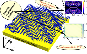
Figure 1: The schematic setup of our model, consisting of a SS state in 2D square lattice, a natural ground state of a magnetic layer grown on the surface of an $s$-wave SC. Two possible experimental schemes to probe MFEM: the momentum space probe (e.g., ARPES), where one obtains the spectral function as a signature of the MFEM, see right top image and the real space probe (e.g., STM), where one obtains spatial distribution of the MFEM at edges, see the right bottom image.

Recently, theoretical proposals for the 2D Kitaev model with topological gapless phase hosting MFEMs has been put forward by employing $(p_{x}$+$p_{y})$-SCs Wang et al. (2017); Zhang et al. (2019). In other existing models, a few schemes using inhomogeneous magnetic fields, various magnetic orders $etc$ were also explored to generate different $p$-wave pairing Sedlmayr et al. (2015); Nakosai et al. (2013); Chen and Schnyder (2015). Although a formal connection between these two schemes involving both model and real materials, manifesting similar behavior has never been proposed. Most importantly, examples with properly designed materials carrying MFEM in the TSC phase have not been explored, neither in theory nor experiment. Moreover, of particular interest is the noncollinear spin-spiral (SS) solutions in 2D, whose presence in the magnet/superconductor heterostructures is highly desirable for the TSC phase. Hence, we can address the following intriguing questions that have not been answered so far to the best of our knowledge: (a) Can we architect and identify magnetic heterostructures where the SS solution in the presence of $s$-wave SC exhibits features of 2D Kitaev model? (b) Is it possible to derive/invoke an effective continuum model consisting of an induced effective spin-orbit coupling (SOC) and Zeeman field to describe such system? (c) Finally and the most importantly, can we identify prototype magnetic heterostructures where the SS ground state exhibits gapless TSC phase hosting MFEM within a lattice model? By stabilizing the SS state in 2D films comprising of 3$d$ transition metal (TM) monolayer and $s$-wave SC substrate may offer the most promising platform for stabilizing the TSC phase in experiments.

In this letter, we first deal with the 2D spin textures in the form of SSs, mimicking spatially varying magnetic impurities placed on the top of a $s$-wave SC substrate. An effective $(p_{x}+p_{y})$-SC pairing is identified for the SS along the [110] direction in a 2D square domain, manifesting a gapless TSC phase. At the end, afterall, the designed TM/SC heterostructure must reveal SS state as the ground state spin texture. We design potential material candidates: one monolayer of Mn and Cr on Nb(110) and Nb(001) $s$-wave SC substrates, respectively. A very recent experiment suggests that the Mn/Nb(110) shows in-gap YSR band, owing to the proximity induced SC state in the antiferromagnetic (AFM) phase. Lo Conte et al. (2022). Indeed, we find the in-gap YSR bands for the AFM phase, obtained within ab initio calculations using optimized lattice constant of Nb. We take advantages of such good agreement with the experimental findings and other aspects of 2D noncollinear magnets Nandy et al. (2016). Under uniform biaxial compressive strain, the AFM-SS state is found to be the ground state for the Mn/Nb(110). The SS texture of Mn/Nb(110) within a lattice model now shows a robust TSC phase hosting MFEM localized at the [110] edges. The TSC phase is also found in the other TM/SC example, Cr/Nb(001). Hence, this real material platform adds significant merit to the problem we are dealing with.

Formulation of 2D Kitaev continuum model.— Within a continuum model, we first propose a general route to design 2D gapless TSC phase via engineering SS textures, proximitized with an $s$-wave SC. Here, the 2D model Hamiltonian in the presence of locally varying magnetic impurities reads in the Nambu spinor form, $\Psi(\boldsymbol{\mathrm{r}})$=$\begin{pmatrix}c_{\boldsymbol{\mathrm{r}},\uparrow},\!&\!c_{\boldsymbol{\mathrm{r}},\downarrow},\!&\!c^{\dagger}_{\boldsymbol{\mathrm{r}},\downarrow},\!&\!\!-c^{\dagger}_{\boldsymbol{\mathrm{r}},\uparrow}\end{pmatrix}^{\rm T}\!$ as $\mathcal{H}_{2{\rm D}}$=$\int\!d\boldsymbol{\mathrm{r}}\Psi^{\dagger}(\boldsymbol{\mathrm{r}})~{}H~{}\Psi(\boldsymbol{\mathrm{r}})$, where $c_{\boldsymbol{\mathrm{r}},\uparrow(\downarrow)}$ represents the quasiparticle annihilation operator for the up (down) spin at $\boldsymbol{\mathrm{r}}$=$(x,y)$ of a 2D SC. The first quantized form of this Hamiltonian reads,

$$H= -\frac{1}{2}\boldsymbol{\mathrm{\nabla}}^{2}\tau_{z}-J\boldsymbol{\mathrm{S}}(\boldsymbol{\mathrm{r}})\cdot\boldsymbol{\sigma}+\Delta_{0}\tau_{x}-\mu\tau_{z}\ .$$ (1)

For simplicity, we consider $\hbar$=$1$ and $m$=$1$. The Pauli matrices $\sigma$ and $\tau$ acts on the spin and particle-hole subspace, respectively. Here, $J$ denotes the local exchange-interaction strength between the magnetic impurity spin and electrons in the SC, $\Delta_{0}$ is the $s$-wave SC order parameter, and $\mu$ is the chemical potential. We assume the impurity spin to be classical with magnitude, $\lvert\boldsymbol{\mathrm{S}}\rvert$=$1$, and confined in the $xy$-plane. Therefore, spin vector $\boldsymbol{\mathrm{S}}(\boldsymbol{\mathrm{r}})$ can be locally described as $\boldsymbol{\mathrm{S}}(\boldsymbol{\mathrm{r}})$=$\lvert\boldsymbol{\mathrm{S}}\rvert\begin{pmatrix}\cos[\phi(\boldsymbol{\mathrm{r}})],\!&\!\sin[\phi(\boldsymbol{\mathrm{r}})],\!&\!0\end{pmatrix}$ with $\phi(\boldsymbol{\mathrm{r}})$, the angle between two adjacent spins. By introducing a unitary transformation $U$=$e^{-\frac{i}{2}\phi(\boldsymbol{\mathrm{r}})\sigma_{z}}$, an effective low-energy Hamiltonian $\tilde{H}$=$U^{\dagger}HU$ in 2D is now,

$$\tilde{H}\!=\! -\frac{1}{2}\!\!\sum_{r_{i}=x,y}\!\!\left[\!\nabla_{r_{i}}^{2}\!-\!\left(\!\partialderivative{\phi}{r_{i}}\!\right)^{\!2}\!\!-\!\left(\!i\partialderivative{\phi}{r_{i}}\nabla_{r_{i}}\!+i\nabla_{r_{i}}\partialderivative{\phi}{r_{i}}\right)\!\sigma_{z}\!\right]\!\tau_{z}$$

$$~{}~{}~{}~{}~{}~{}~{}~{}~{}~{}~{}~{}~{}~{}~{}~{}~{}~{}~{}~{}~{}~{}~{}~{}~{}~{}~{}~{}~{}~{}~{}~{}~{}+\!J\sigma_{x}\!+\!\Delta_{0}\tau_{x}\!-\!\mu\tau_{z}\ .$$ (2)

Note, the similar mapping was reported for 1D spin chain model in case of Majorana bound state solution Hess et al. (2022).

Henceforth, we assume the propagation direction of the SS is along the diagonal of a square domain $i.e.$ along an effective [110] direction as depicted in Fig. 1. The angle, $\phi(\boldsymbol{\mathrm{r}})$=$\boldsymbol{\mathrm{g}}\!\cdot\!\boldsymbol{\mathrm{r}}$=$\left(g_{x}x+g_{y}y\right)$, defines the angle between two adjacent spins along the SS propagation direction where $g_{x}$ and $g_{y}$ can be tuned to control the SS period and propagation direction. A homogeneous SS perfectly moving along either [110] or [1$\bar{1}$0] directions (depending on the sign of $g_{x}$ and $g_{y}$) occurs when the components of $\boldsymbol{\mathrm{g}}$ are equal in magnitude. In general ($|g_{x}\rvert\!\!\neq\!\!|g_{y}\rvert$) cases when the asymmetric spin textures with the SS propagating other than [110], [1$\bar{1}$0] directions, the Hamiltonian $\tilde{H}$ in Eq. (2) can be rewritten in the momentum space as

$$\tilde{H}(\boldsymbol{\mathrm{k}})\!=\! \xi_{\boldsymbol{\mathrm{k}},\boldsymbol{\mathrm{g}}}\tau_{z}\!+\!\frac{1}{2}\boldsymbol{\mathrm{g}}\!\cdot\!\boldsymbol{\mathrm{k}}\ \sigma_{z}\tau_{z}\!+\!J\sigma_{x}\!+\!\Delta_{0}\tau_{x}\ ,$$ (3)

where, $\xi_{\boldsymbol{\mathrm{k}},\boldsymbol{\mathrm{g}}}$=$\frac{1}{2}\left(\boldsymbol{\mathrm{k}}^{2}\!+\!\boldsymbol{\mathrm{g}}^{2}\right)\!-\!\mu$. The second term turns out to be an effective SOC, resulting from the spin texture in our model. Although, the nature of such SOC is quite nontrivial as it originates from the spin texture, it can interestingly give rise to a gapless TSC phase hosting MFEM in the presence of Zeeman like field of strength $J$ along the $x$-direction. We obtain the spectrum for the Hamiltonian $\tilde{H}(\boldsymbol{\mathrm{k}})$ in Eq. (3) as, $E_{r,s}(\boldsymbol{\mathrm{k}},\boldsymbol{\mathrm{g}})$=$r\sqrt{J^{2}\!+\!\Delta_{0}^{2}\!+\!\xi_{\boldsymbol{\mathrm{k}},\boldsymbol{\mathrm{g}}}^{2}\!+\!\frac{1}{4}\boldsymbol{\mathrm{k}}\cdot\boldsymbol{\mathrm{g}}+sF(\boldsymbol{\mathrm{k}},\boldsymbol{\mathrm{g}})}$; where, $r,s$=$\pm$ and $F(\boldsymbol{\mathrm{k}},\boldsymbol{\mathrm{g}})$=$\sqrt{[(\boldsymbol{\mathrm{k}}\cdot\boldsymbol{\mathrm{g}})^{2}\!+\!4J^{2}]^{2}\xi_{k,g}^{2}\!+\!4J^{2}\Delta_{0}^{2}}$. Following the gap closing condition corresponding to the two lowest energy bands, the critical value of the exchange coupling strength $J$ becomes $J_{c}(\boldsymbol{\mathrm{g}})$=$\sqrt{\Delta_{0}^{2}\!+\!\left(\mu\!-\!\boldsymbol{\mathrm{g}}^{2}/2\right)^{2}}$. The period of the SS now can be manifested like $T$=$\pi/|\boldsymbol{\mathrm{g}}\rvert$=$\pi/\!\sqrt{g_{x}^{2}\!+\!g_{y}^{2}}$ Hess et al. (2022). Hence, in case of $|g_{x}\rvert$=$|g_{y}\rvert$=$g$, the period turns out to be $T$=$\pi/\sqrt{2}g$. Naively, the SS solution is governed by the RKKY-type (Ruderman-Kittel-Kasuya-Yosida) exchange frustration in the presence of free electrons and if the period of SS is set by the Fermi momentum $\boldsymbol{\mathrm{k}}_{F}$, then $T$=$\pi/\lvert\boldsymbol{\mathrm{g}}\rvert$=$\pi/\lvert\boldsymbol{\mathrm{k}}_{F}\rvert$ Hess et al. (2022); Klinovaja et al. (2013); Braunecker and Simon (2013); Vazifeh and Franz (2013). In such case, the topological transition occurs at $J_{c}$=$\Delta_{0}$ so that $\mu$=$|\boldsymbol{\mathrm{k}}_{F}\rvert^{2}/2$. However, in real TM/SC films, the SS solution is the outcome of a complex interplay of material dependent parameters like exchange coupling constants, $\mathcal{J}_{ij}$’s; Dzyaloshinskii-Moriya Interactions (DMIs), $\mathcal{D}_{ij}$’s; and uniaxial magnetic anisotropy constant, $\mathcal{K}$ as discussed later in the context of 2D Kitaev lattice model.

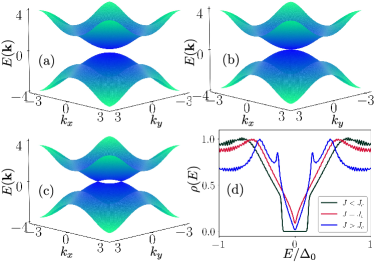
Figure 2: The bulk band structures of the Hamiltonian $\tilde{H}_{\rm L}(\boldsymbol{\mathrm{k}})$ in the $k_{x}$-$k_{y}$ plane is depicted for (a) the trivially gapped SC phase, $J<J_{c}$ (=1.6$\Delta_{0}$), (b) the gap closing transition point, $J=J_{c}$ (=1.77$\Delta_{0}$), and (c) the gapless TSC phase hosting MFEM, $J>J_{c}$ (=2.0$\Delta_{0}$). (d) TDOS, $\rho(E)$, is shown as a function of $E/\Delta_{0}$ for the above mentioned $J$ values in the parenthesis. All remaining parameters take values: $g_{x}$=$g_{y}$=$\pi/2$, $\mu$=$\Delta_{0}=t$.

The band structure of this system has been analyzed using the lattice version of the Hamiltonian $\tilde{H}(\boldsymbol{\mathrm{k}})$ [Eq. (3)] defined as $\tilde{H}_{\rm L}(\boldsymbol{\mathrm{k}})$ (see Eq. (S1) in Section S1 of the supplementary materials (SM) sup ). We depict the bulk band structure of $\tilde{H}_{\rm L}(\boldsymbol{\mathrm{k}})$ and the corresponding total density of states (TDOS) $\rho(E)$ in Fig. 2 for different values of $J$. The topological phase transition occurs between a normal SC phase with a trivial gap as shown in Fig. 2(a) for $J\!\!<\!\!J_{c}$ to the gapless TSC phase in Fig. 2(c) for $J\!\!>\!\!J_{c}$ via a gap closing phase at $J$=$J_{c}$ (=1.77$\Delta_{0}$) as depicted in Fig. 2(b). The topological characterization via appropriate topological invariant ($\nu$) is provided in the SM sup . The change in $\nu$ from $0$ to $1$ occurs when the system makes the transition from a trivial gaped state ($J\!\!<\!\!J_{c}$) to a non-trivial ($J\!\!>\!\!J_{c}$) TSC phase. This gapless phase displays graphene like semimetalic behavior Castro Neto et al. (2009); Wakabayashi et al. (2010) where $\rho(E)$ corresponding to the gapless TSC phase ($J\!\!>\!\!J_{c}$) varies almost linearly with $E$ (see Fig. 2(d)). The band structure illustrated in Fig. 2(c) resembles that of the 2D Kitaev model in the TSC phase, reported recently in Refs. Zhang et al. (2019); Wang et al. (2017). There, the idea of 2D Kitaev model hosting MFEM has been analytically formulated considering ($p_{x}+p_{y}$)-SCs. Thus, we can infer that an effective ($p_{x}+p_{y}$) SC pairing is generated in our system due to a proper domain of SSs propagating along the [110] direction, when proximitized with a $s$-wave SC. These results seemingly ensure that the crucial prerequisite for the TSC phase hosting MFEM is the noncollinear SS state stabilized in TM/SC systems.

In a slab geometry where the system is finite along the $y$-direction and periodic along the $x$-direction, we calculate the spectral function, $\mathcal{A}(k_{x},\omega)$ spe . In Fig. 3, we show the behavior of $\mathcal{A}(k_{x},\omega)$ as a function of energy $\omega/\Delta_{0}$. Indeed, in Fig. 3(c), a clear signature of the MFEM is found in the gapless TSC phase and Fig. 3(a) does not show any signature of MFEM, except a trivial gap. However, $\mathcal{A}(k_{x},\omega)$ in Fig. 3(b) for $J$=$J_{c}$ shows the edge modes which are still infinitesimally gaped. Experimentally, one can probe these signatures of TSC phase using ARPES measurements but such a small gap close to the transition point will be impossible to resolve.

2D Kitaev lattice model for TM/SC heterostructure.— We now focus on the realistic materials framework to rationalize the above described phenomena. We, therefore, design two prototype TM/SC heterostructures where the magnetic layer based on 3$d$-TM elements (Mn and Cr) is proximitized by $s$-wave SC substrates, Nb(110) and Nb(001), respectively. We numerically solve for their ground state magnetic textures within Monte Carlo (MC) simulations Landau and Binder (2000); MC_ ; Bera and Mandal (2019, 2021). The Hamiltonian is comprised of contributions from material-specific parameters, $\mathcal{J}_{ij}$’s, $\mathcal{D}_{ij}$’s and $\mathcal{K}$ Müller et al. (2019); Heo et al. (2016); Flovik et al. (2017), calculated within ab initio electronic structure simulations (see Section S2) in the SM sup ).

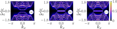
Figure 3: In panels (a)-(c) we show the density plots of the spectral function $\mathcal{A}(k_{x},\omega)$ in the $k_{x}-\omega$ plane. An explicit signature of the MFEM can be seen in panel (c) for $J>J_{c}$ (=2.0$\Delta_{0}$) where the bulk is a gapless TSC. We choose the same set of respective parameters as mentioned in Fig. 2.

The optimized 2D lattice of Mn/Nb(110) opt indeed show a $c(2\times 2)$ AFM order as the ground state which is recently reported by Conte $et~{}al.$ Lo Conte et al. (2022), see the SM, Section S3(A) for detail results sup . Surprisingly, a transition to an AFM-SS state occurs via a uniform biaxial compressive strain within the range, $\sim-1$ to $-4$ %. Considering $a$=3.234 Å and $b$=$\sqrt{a}$=4.574 Å (strain ​ $\sim\!-2.7$ %), Fig. 4(a) illustrates $\mathcal{J}_{ij}$’s and the absolute values of DMI vectors ($\mathcal{D}_{ij}$) as a function of the distance between Mn atoms and here, $\mathcal{K}$ is found to be positive i.e.,  out-of-plane. The inset describes the vector orientations of DMI connecting neighboring atoms that match the symmetry rules for a system with $\mathcal{C}_{2v}$ symmetry Moriya (1960). More details of calculations and results for both planner compression and expansion of Mn/Nb(110) film are provided in the SM, Section S3(B) sup . The AFM-SS is found to be the ground state even without considering DMI, resulting from the strong frustration in $\mathcal{J}_{ij}$’s between magnetic moments on Mn ($\mathcal{M}_{\textrm{Mn}}$= 3.53 $\mu_{\textrm{B}}$). A DMI with weak strength ($<\!0.5~{}meV$) is attributed to the light atom based films (weak SOC) and it determines the handedness of the SS rotation (a right-handed cycloidal AFM-SS) along with an expected small decrease in the SS period ($\lambda_{\textrm{Mn}}$ changes from $\approx$ 2.82 $nm$ to $\approx$ 2.35 $nm$). The SS is propagating along the [010] direction, see Fig. 4(b). In contrast, the AFM-SS earlier reported in Mn/W(110), a non-SC film system, where a strong DMI determines the left-rotating spin cycloid, owing to the strong SOC from the heavy metal element W Bode et al. (2007).

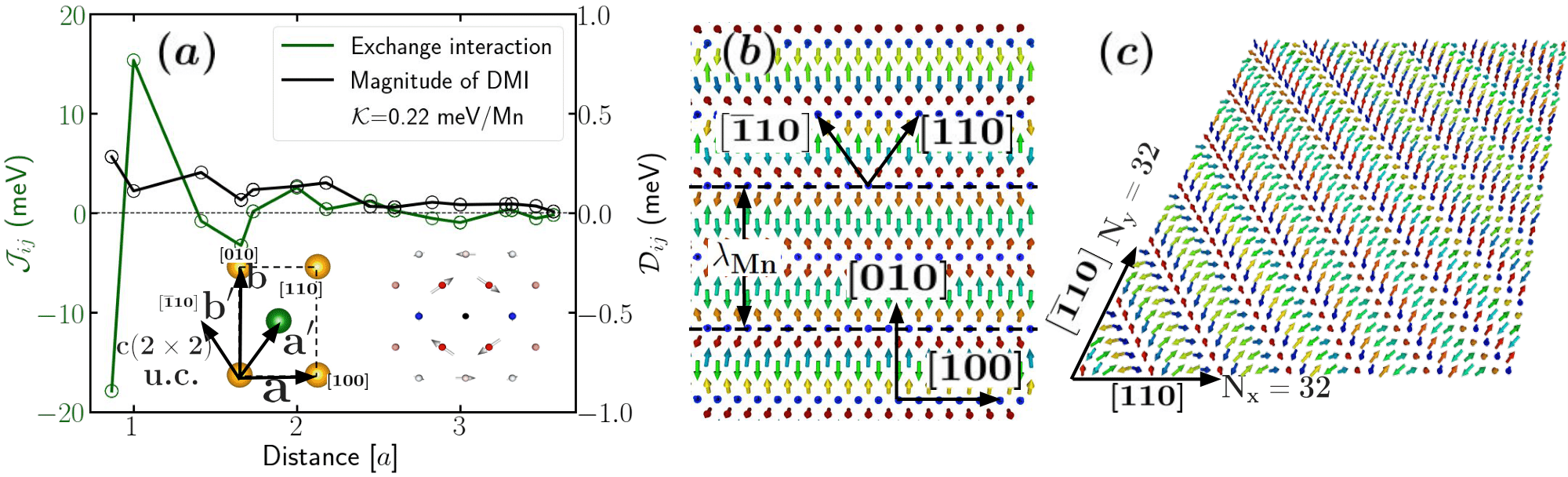
Figure 4: For Mn/Nb(110) with strain $\sim\!\!-2.7$%, (a) $\mathcal{J}_{ij}$’s and $\mathcal{D}_{ij}$’s are plotted as a function of distance measured in units of lattice constant $a$. $\mathcal{K}$ is found to be out-of-plane. Lower left inset shows the $c(2\times 2)$-AFM surface unit cell (which possesses $\mathcal{C}_{2v}$ symmetry) , yellow ball (up-spin) and green ball (down-spin) or vice versa and the lower right inset describe vector-orientations of DMI. (b) The AFM-SS ground state (by MC simulations) propagates along the [010] direction. (c) A $32\times 32$ magnetic lattice domain with AFM-SS is shown where edges are along [110] and [$\bar{1}$10] directions.

Here, we elucidate a minimal electronic model Hamiltonian in real space for a 2D lattice,

$$H = \!-\!\!\sum_{\langle i,j\rangle,\alpha}t_{ij}c_{i,\alpha}^{\dagger}c_{j,\alpha}\!-\!\mu\sum_{i,\alpha}c_{i,\alpha}^{\dagger}c_{j,\alpha}$$ (4)

$$+J\!\!\sum_{i,\alpha,\beta}\!\!c_{i,\alpha}^{\dagger}\!\left(\boldsymbol{\mathrm{\hat{s}}}_{i}\!\cdot\!\boldsymbol{\mathrm{\sigma}}\right)_{\alpha,\beta}c_{i,\beta}\!+\!\Delta_{0}\!\sum_{i}(c_{i,\uparrow}^{\dagger}c_{i,\downarrow}^{\dagger}\!+\!{\rm H.c.})\ ,\quad~{}\$$

where, the indices $i,j$ run over all the lattice sites, $\alpha,\beta$ denote the spin, $\langle\rangle$ represents nearest-neighbor hopping only and $\mu$, $J$, $\Delta_{0}$ represent the chemical potential, exchange coupling strength, $s$-wave SC gap, respectively. Here, $c^{\dagger}$ ($c$) corresponds to the electron creation (annihilation) operator for the superconductor. For simplicity, we assume the hopping amplitude $t_{ij}$=$t_{ji}$=$-t$ and set $t$=1 for the overall energy scale of our system. This minimal Hamiltonian is essentially constructed to ensure the importance of magnetic textures (alternative to the intrinsic SOC) of TM/SC heterostructures in the context of stabilizing TSC phase. All spin textures are actually entered in the third term in the Eq. (4), describing a local interaction between the electron’s spin ($\sigma$) and the moments of Mn or Cr. The unit vector $\boldsymbol{\mathrm{\hat{s}}}_{i}$ denotes $(\sin\theta_{i}\cos\phi_{i},\sin\theta_{i}\sin\phi_{i},\cos\theta_{i})$, mimicking locally varying magnetic impurities in 2D. One can extract these $\theta$ and $\phi$ from the spin textures generated by the MC simulations for TM/SC systems.

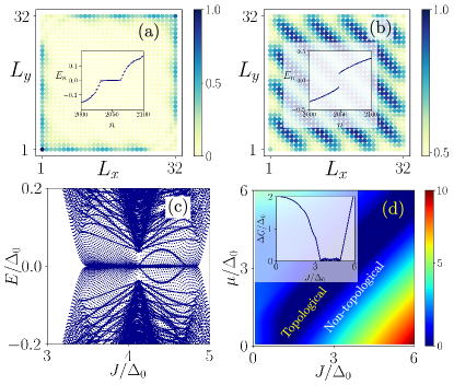
Figure 5: We depict the normalized LDOS for $E$=0 eigenstate, computed within a spin lattice model of size 32$\times$32 spins, $L_{x}\mathchar 45\relax L_{y}$ square plane. Here, lattice points (vectors) are represented in unit of the rotated vectors, $\boldsymbol{\mathrm{a^{\prime}}}$ and $\boldsymbol{\mathrm{b^{\prime}}}$, as shown in the inset of Fig. 4(a). For Mn/Nb(110) with AFM-SS state at $J$= 4.5$\Delta_{0}$, (a) we identify the TSC phase. The LDOS is predominantly localized at the domain edges denoting MFEMs. (b) $J$= 5.0$\Delta_{0}$ identifies the trivial phase where LDOS is delocalized over the entire domain. Insets in (a) and (b) clearly show a zero-energy flat mode and a trivial gap, respectively in the eigenvalue spectrum ($E_{n}$) vs. state ($n$) plots. (c) The plot of energy eigenvalues $E$ of $H$ is shown as a function of $J$ using open boundary condition. (d) The bulk-gap $\Delta G$ profile is depicted in the $J\mathchar 45\relax\mu$ plane employing periodic boundary condition. The dark blue regime represent the TSC phase. The inset demonstrates the $\Delta G$ as a function of $J$ for a fixed $\mu$. We choose $\mu$=4.0$\Delta_{0}$ and $\Delta_{0}$=$t$.

In case of Mn/Nb(110), the $c(2\times 2)$ AFM phase has been assessed first via numerically solving Eq. (4). The Hamiltonian indeed describes the experimental findings where the $s$-wave SC and AFM phases coexist Lo Conte et al. (2022). Results in detail presented in the SM, Section S3(B) sup which reveals the in-gap YSR bands, ensuring qualitative accuracy of our minimal model described in Eq. (4).

We now discuss a few important results obtained from the numerical simulations by considering the 2D AFM-SS domain. For a proper domain of SS texture where the propagation direction is along the diagonal of that domain, the AFM-SS solution has been used to construct a particular domain of size 32$\times$32 (1024 spins) with edges along [110] and [1$\bar{1}$0] directions (see Fig. 4(c)). These directions are parallel to the rotated vectors $\boldsymbol{\mathrm{a^{\prime}}}$ and $\boldsymbol{\mathrm{b^{\prime}}}$ of the 2D lattice and thereby, the AFM-SS propagates along the diagonal direction of the domain, similar as the FM-SS in Fig. 1. The measured $\theta$ and $\phi$ values are used in $\hat{s}$ for the numerical solutions of Eq. (4). Results are summarized in Figs. 5 where, (a) and (b) depict the local density of states (LDOS) for the zero-energy ($E$=0) states using coupling constant, $J$=4.5$\Delta_{0}$ and 5.0$\Delta_{0}$, respectively. The zero-energy states populate along the edges of the considered domain in Fig. 5(a) and hence, the system is in the TSC regime. The MFEM are maximally localized at the two opposite corners of the system and disperse gradually along the edges. Moreover, the signature of the MFEM are more evident from the non-dispersive states at $E_{n}$=0 in the eigenvalue spectrum plotted as a function of the state index $n$ in the inset of Fig. 5(a). Furthermore, the semimetallic behavior of the bulk YSR band at $J$ = 4.5$\Delta_{0}$ (see SM, Section S5 for details) sup in the TSC regime qualitatively matches with the continuum results presented in Fig. 2(d). In the inset of Fig. 5(b), a trivial phase on the other hand appears with a gap in that spectrum around $E_{n}$=0.

Seemingly, it appears that the coupling constant $J$ (rather, $J/\Delta_{0}$) plays a major role in the phase transition between trivial SC and TSC phases. Particularly, $J$ value is often very challenging to determine for such materials. Therefore, in Fig. 5(c), we depict the eigenvalue spectrum $E/\Delta_{0}$ as a function of $J/\Delta_{0}$ by employing open boundary condition. The MFEM appears at zero-energy between $J$=3.5$\Delta_{0}$ and $J$=4.7$\Delta_{0}$, indicating the TSC regime. We thereafter identify the parameter regime where the MFEM appears via calculating the bulk-gap, $\Delta G$=$\lvert E_{2}$-$E_{1}\rvert$, within periodic boundary condition. Here, $E_{1}$ ($E_{2}$) represents the two low energy bands. We depict $\Delta G/\Delta_{0}$ in the $J/\Delta_{0}\mathchar 45\relax\mu/\Delta_{0}$ plane in Fig. 5(d). The gapless TSC regime harboring MFEM is highlighted by the dark blue strip ($\Delta G\simeq 0$), while the regime outside ($\Delta G>0$) represents gapped trivial superconducting phase. In the inset of Fig. 5(d), we illustrate the bulk-gap $\Delta G$ as a function of $J$ for a fixed value of $\mu$, for the transparent visibility of the TSC regime. The bulk-gap $\Delta G$ vanishes in the topological regime and MFEM appears at the boundary. Therefore, our study with a wide variation in noncollinear AFM spin textures firmly establish the non-trivial TSC phase hosting MFEM, allowing a formal connection between noncollinear magnetism in real materials and model studies.

We further construct a new TM/SC magnetic ultrathin film, Cr/Nb(001), where a different type of AFM-SS ground state is observed without strain. For the shake of completeness, we study the surface strain effect and the detail results are presented in the SM, Section S4 sup . In contrast to the Mn/Nb(110) system, two degenerate chiral AFM-SS (left-handed cycloid propagating along [100] and [010] directions) states are found, owing to the symmetry rules followed by the DMI vectors in the $\mathcal{C}_{4v}$ symmetric system Moriya (1960). We solve Eq. (4) again for the square domains as shown in Fig. S5(c) and (e) while the respective LDOSs are shown in Fig. S6(a) and (b). One of the major findings is that the location of MFEM depends on the propagation direction of the SS. So, one can infer that the MFEM can be probed experimentally at any edge of a square domain containing both propagating SSs.

Summary and outlook.— In conclusion, by employing a continuum model, we demonstrate a route to generate a gapless TSC phase hosting MFEMs by engineering noncollinear SS state proximitized with an $s$-wave superconductor. This underlying scheme is later extended within a minimal lattice model which provides a unique way to unveil the TSC phase in prototype real TM/SC ($s$-wave) materials: Mn/Nb(110) under strain and Cr/Nb(001). Even though, the SOC strength in Nb is expected to be very small, the AFM-SS can be stabilized from the exchange frustration, particularly in the Mn/Nb(110) sample and thereby, an effective SOC and Zeeman filed terms due to the spin textures manifest the Hamiltonian obtained in  Eq. (3). Our realistic model Hamiltonian unveils excellent examples where the strain driven modulation of the noncollinear magnetic phases can offer unprecedented control over the TSC phase mimicking 2D Kitaev model. Particularly, various noncollinear AFM order and their control Salemi et al. (2019) in future can become a remarkable way of tuning various TSC phases for e.g., dispersive Majorana edge modes, higher-order topological superconducting phase hosting Majorana corner modes etc. This will also be an important step towards applications in AFM-SC spintronics and topological quantum computation.

Acknowledgments.— The first-principle calculations in this letter is supported by the Swedish National Infrastructure for Computing (SNIC) facility and for that, S.B. and A. K. N. sincerely thank Prof. P. M. Oppeneer. P.C., S.B, A.K.G., A.S. and A. K. N. acknowledge the support from Department of Atomic Energy (DAE), Govt. of India. S B. and A.K.N. acknowledge the KALINGA HPC facility at NISER, Bhubaneswar and P.C., A.K.G. and A.S. acknowledge the SAMKHYA: HPC Facility provided at IOP, Bhubaneswar, for numerical computations.

S1 Topological characterization

In this section of the supplementary material (SM), we discuss the topological characterization of our model. We begin with the continuum Hamiltonian described in the main text [Eq. (3)]. One can obtain the lattice version of the continuum Hamiltonian by replacing $k_{x}\to\sin k_{x}$, $k_{y}\to\sin k_{y}$, $(1-k_{x}^{2}/2)\to\cos k_{x}$, and $(1-k_{y}^{2}/2)\to\cos k_{y}$ as

$$\tilde{H}_{\rm L}(\boldsymbol{\mathrm{k}})= \xi_{\boldsymbol{\mathrm{k}},\boldsymbol{\mathrm{g}}}\tau_{z}+\frac{1}{2}(g_{x}\sin k_{x}+g_{y}\sin k_{y})\sigma_{z}\tau_{z}+J\sigma_{x}+\Delta_{0}\tau_{x}\ ,$$ (S1)

where, $\xi_{\boldsymbol{\mathrm{k}},\boldsymbol{\mathrm{g}}}=(2-\cos k_{x}-\cos k_{y})+\frac{(g_{x}^{2}+g_{y}^{2})}{2}-\mu$. At the high symmetry points $\boldsymbol{\mathrm{\Gamma}}_{l}=[(0,0),(\pi,0),(0,\pi),(\pi,\pi)]$, if we perform the proper basis transformation, then the Hamiltonian in Eq. (S1) can be recast in the block diagonal form as,

$$\tilde{H}_{\rm L}(\boldsymbol{\mathrm{k}}) =\begin{pmatrix}h(\boldsymbol{\mathrm{\Gamma}}_{l})&O_{2\times 2}\\ O_{2\times 2}&-h(\boldsymbol{\mathrm{\Gamma}}_{l})\end{pmatrix}\ .$$ (S2)

where,

$$h(\boldsymbol{\mathrm{\Gamma}}_{l}) =\begin{pmatrix}J+\xi_{\boldsymbol{\mathrm{k}},\boldsymbol{\mathrm{g}}}(\boldsymbol{\mathrm{\Gamma}}_{l})&\Delta_{0}\\ \Delta_{0}&J-\xi_{k,g}(\boldsymbol{\mathrm{\Gamma}}_{l})\end{pmatrix}\ .$$ (S3)

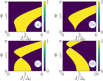
Figure S1: Topological invariant $\nu$ for the symmetric ($g_{x}=g_{y}=\Phi$) spin texture is shown. Panels (a), (b), (c), and (d) correspond to the variation of $\nu$ in the $J\mathchar 45\relax\Phi$ plane for different values of the chemical potential $\mu=\Delta_{0},2.0\Delta_{0},4.0\Delta_{0}$, and $8.0\Delta_{0}$, respectively.

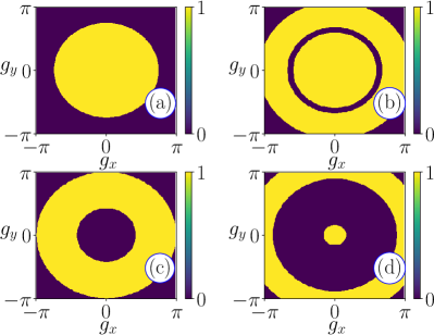
Figure S2: Topological invarient $\nu$ in case of asymmetric spin texture ($g_{x}\neq g_{y}$) is depicted. Panels (a), (b), (c), (d) correspond to the variation of $\nu$ in $g_{x}-g_{y}$ plane, where we choose the other parameter values for panels (a), (b) are $J=2.0\Delta_{0},\mu=\Delta_{0}$ and $J=2.0\Delta_{0},\mu=4.0\Delta_{0}$ respectively. On the other hand, for panels (c), (d) we choose $J=4.0\Delta_{0},\mu=\Delta_{0}$ and $J=4.0\Delta_{0},\mu=4.0\Delta_{0}$ respectively.

The topological invariant reads Sedlmayr et al. (2015),

$$\delta ={\rm sgn}~{}\prod_{l=1}^{4}\det\begin{pmatrix}J+\xi_{\boldsymbol{\mathrm{k}},\boldsymbol{\mathrm{g}}}(\boldsymbol{\mathrm{\Gamma}}_{l})&\Delta_{0}\\ \Delta_{0}&J-\xi_{\boldsymbol{\mathrm{k}},\boldsymbol{\mathrm{g}}}(\boldsymbol{\mathrm{\Gamma}}_{l})\end{pmatrix}\ =(-1)^{\nu}\ ,$$ (S4)

where the quantity $\nu$ is treated as a topological invariant. Therefore, one can identify the topologically trivial and non-trivial regime by considering $\nu=0$ or $\nu=1$ accordingly. In Fig.(S1) and Fig.(S2) we illustrate the topological invariant considering symmetric and asymmetric spin spirals (SS) in different parameter regimes. In each figure (Figs. S1 and S2), the yellow region indicates the gapless topological superconducting (TSC) phase ($\nu=1$) hosting Majorana flat edge modes (MFEM) due to the generation of an effective $(p_{x}+p_{y})$ type of superconducting pairing. On the other hand, in the violet region, the system becomes a topologically trivial gapped superconductor ($\nu=0$), where MFEM disappear due to the destruction of the $(p_{x}+p_{y})$ type pairing.

S2 Methodology

In this section, we discuss the computational details for extracting the material specific parameters within ab initio electronic structure calculations. All these parameters are for various heterostructures made of an atomic-layer-thick magnetic layer of 3$d$ transition metal (TM) elements, Mn and Cr, on the top of normal $s$-wave superconducting substrate. A body-centred-cubic ($bcc$) Nb with different surface cuts, (110) and (001) is used as the substrate. Ultimately, these parameters are used for generating ground state spin texture by solving extended Heisenberg model within Monte Carlo (MC) simulations, which is the essential ingredient for establishing the topological superconducting (TSC) phase.

S2.1 Film geometry relaxation within ab initio electronic structure method

We first begin with the optimized lattice of bulk $bcc$-Nb superconductor. The optimized lattice constant of bulk $bcc$-Nb has been obtained by performing first-principles electronic structure calculations within the density-functional theory and the plane-wave pseudopotential approach as implemented in the Vienna Ab-initio Simulation Package (VASP)Hafner (2008); Kresse and Furthmüller (1996, 1996). Exchange and correlation have been considered within the generalized gradient approximation (GGA) which is parametrized via Perdew, Burke, and Ernzerhof (PBE) functional Perdew et al. (1996). Here, the projector-augmented wave (PAW) method is employed to construct the pseudopotentials with valence wavefunctions which are approximated smooth near ion cores Kresse and Joubert (1999); Blöchl (1994). The plane wave cut-off energy (500 $\rm eV$) and the $k$-point mesh (16$\times$16$\times$16 and $\Gamma$-centred) in the full Brillouin-zone (BZ) are checked carefully for the BZ integration, ensuring the numerical convergence of self-consistently determined quantities. The optimised lattice constant of $bcc$-Nb is found to be $a_{\textrm{opt}}$=3.3232 Å, matching well with the experimental value in the Materials Project database ($a_{\textrm{expt}}$=3.32 Å) Project .

The surface unit cell (u.c.) in the form of two-dimensional (2D) slab geometry is constructed with sufficiently thick vacuum layers. The thickness of vacuum on each side of the slab is taken about 10 Å. Assuming a pseudomorphic layer by layer growth, ultrathin magnetic films are constructed by considering a single layer of Mn and Cr on a well known $s$-wave superconductor (SC) substrates Nb(110) and Nb(001), respectively. In case of Mn/Nb(110) film, each surface layer contains two atoms and the thickness of the substrate is taken 11 monolayers (MLs), see Fig. S3(a). In the Cr based film as depicted in Fig. S5(a), one atom per layer is repeated along $c$-axis with the substrate thickness of about 15 MLs. The surface u.c. parameters using optimized $bcc$-Nb lattice constants are $a$= 3.3232 Å with $b/a$=$\sqrt{2}$ and $a$=$b$=3.3232 Å for Mn/Nb(110) and Cr/Nb(001) magnetic films, respectively. Increasing the layer numbers beyond that doesn’t carry any effect on the properties of the systems. Later, uniform biaxial strain has been calculated with respect to the optimized lattice constant as, strain=$\frac{a-a_{\textrm{opt}}}{a_{\textrm{opt}}}\!\times\!100\%$. Therefore, the sign of strain in case of expansion (compression) is positive (negative). The number of MLs in the substrate and the vacuum thickness for all film structures with both compressive and tensile strains are kept fixed. We have used the same energy cut-off for the plane waves and the 12$\times$8$\times$2 $k$-mesh for the BZ integration. The distances between different layers counting from the top TM layer till the 8^th layer (7 interlayer distances) in all films are relaxed until the Hellmann-Feynman force on each atom is smaller than 0.001 $\rm{eV}$/Å. So, we have applied both positive and negative values of strain ($<5\%$) on both Mn/Nb(110) and Cr/Nb(001) films and relaxed each of them along the growth direction. We find that further relaxation with more layers ($>$ 8) does not change the computed results significantly. In every calculations, the self-consistent energy has been converged with an accuracy of 10${}^{-7}~{}\rm{eV}$.

In Table 1 and 2, we have provided the theoretical relaxed structure for Mn/Nb(110) and Cr/Nb(001) magnetic films, respectively. The top Mn and Cr layers are assigned with the number $n$=0 in Fig. S3(a) and S5(a), respectively and $n$ increases if one moves down across the film. The relaxed interlayer distances till $n$=4 (first four interlayer separations only) are presented in those Tables and in the parentheses, we provide the changes in % with respect to the ideal interlayer spacing. For example, the ideal interlayer distance in case of Nb(110) and Nb(001) films using the optimized $bcc$-Nb lattice are 2.3499 Å and 1.6616 Å, respectively. It is expected that the changes in interlayer distance (in %) will be more with both negative and positive strains. Note, we have carefully checked the optimum numbers (till $n=6$) of relaxed interlayer distances, beyond that the change in the interested parameters is neglizible.

Lattice constant	$d_{01}$ in Å	$d_{12}$ in Å	$d_{23}$ in Å	$d_{34}$ in Å
in Å($a_{\textrm{strain}}$)	(% change)	(% change)	(% change)	(% change)
3.432 ($a_{+3.3}$)	1.97(+18.8%)	2.24(+7.7%)	2.24( +7.7%)	2.24( +7.7%)
3.366 ($a_{+1.3}$)	2.00(+16.0%)	2.31(+3.1%)	2.29(+11.4%)	2.30(+11.1%)
3.3232 ($a_{0.0}$)	2.03(+13.5%)	2.35(+0.2%)	2.34( +0.3%)	2.35( +0.2%)
3.270($a_{-1.6}$)	2.08(+10.0%)	2.40($-$3.8%)	2.42( $-$4.7%)	2.42( $-$4.7%)
3.234 ($a_{-2.7}$)	2.10( +8.2%)	2.44($-$6.6%)	2.45( $-$7.0%)	2.44( $-$6.6%)
3.200($a_{-3.7}$)	2.14( +5.4%)	2.47($-$9.1%)	2.48($-$9.5%)	2.48( $-$9.5%)

List of Supplementary Short Tables 1 Structural relaxation details for Mn/Nb(110) magnetic film. Here, $d_{nm}$ defines the distance between layers after relaxation. The ‘+ve’ (‘$-$ve’) signs in $d$ signifies that relaxed distance is larger (smaller) than the ideal distance in the film, obtained from $a$ in each case.

Lattice constant	$d_{01}$ in Å	$d_{12}$ in Å	$d_{23}$ in Å	$d_{34}$ in Å
in Å($a_{\textrm{strain}}$)	(% change)	(% change)	(% change)	(% change)
3.432 ($a_{+3.3}$)	1.22(+28.9%)	1.65(+3.6%)	1.55(+9.8%)	1.6(+6.7%)
3.366 ($a_{+1.3}$)	1.29(+23.4%)	1.67(+0.9%)	1.6(+5.4%)	3.65(+1%)
3.3232($a_{0.0}$)	1.31(+21.07%)	1.68(-1.3%)	1.61(+3.1%)	1.66(0.0%)
3.300(a-0.7)	1.30(+21.3%)	1.72(-4.2%)	1.63(+0.1%)	1.67(-1.6%)
3.234 ($a_{-2.7}$)	1.36(+15.89%)	1.74(-7.5%)	1.69(-4.6%)	1.71(5.7%)
3.168 ($a_{-4.7}$)	1.38(+12.88%)	1.78(-12.5%)	1.75(-10.6%)	1.73(-9.5%)

List of Supplementary Short Tables 2 Structural relaxation details for Cr/Nb(110) magnetic film. Here, $d_{nm}$ defines the distance between layers after relaxation. The ‘+ve’ (‘$-$ve’) signs in $d$ signifies that relaxed distance is larger (smaller) than the ideal distance in the film, obtained from $a$ in each case.

S2.2 Extraction of material specific parameters: Korringa-Kohn-Rostokar Green-function (KKR-GF) method

After the structural relaxation of each magnetic film, the relaxed structures are now used for ab initio simulations performed within the scalar-relativistic screened KKR-GF method Bauer with exact description of the atomic cells. This method is based on the multiple-scattering theory Zabloudil et al. that consists of dividing the problem in calculating the electronic structure of a solid into two parts: solving a single-site scattering problem for each atom in isolation, then incorporating the structural information of the solid by solving a multiple-scattering problem. Note, all the magnetic films are enclosed by two vacuum regions with a thickness of about 10 Å on both top and bottom sides.

The local spin density approximation (LSDA) has been considered Vosko et al. (1980). The effective potentials and fields are treated within the atomic sphere approximation (ASA) with an angular momentum cut-off, $l_{\textrm{max}}$=3. The energy integrations are performed using a grid of 38 points along a path of the complex-energy contour with a Fermi smearing value of 473 K. For the necessary $k$ integrations in the 2D BZ, we have chosen 1600 (40×40×1) $k$-points in the full surface BZ for the integration of the Matsubara pole closest to the real axis in order to perform the self-consistency. Within KKR-GF method including spin-orbit coupling, we have first converged the potential self-consistently for each film, with confining the magnetic moments along out-of-plane direction ($z$-direction).

By employing the KKR-GF method, we essentially calculate the following important parameters: the symmetric exchange interaction, $\mathcal{J}_{ij}$’s, the antisymmetric Dzyaloshinskii-Moriya interaction (DMI), $\textbf{D}_{ij}$ ($|\textbf{D}_{ij}|$ = $\mathcal{D}_{ij}$), and the single ion magnetocrystalline anisotropy (MCA), $\mathcal{K}_{i}$. These parameters contribute in the following Heisenberg model Hamiltonian described in Eq. (S5) and finally, the numerical solutions within MC simulations describe the magnetic textures in the magnetic layer.

$$\mathcal{H} =-\sum_{i>j}\big{[}\!\mathcal{J}_{ij}\hat{n}_{i}.\hat{n}_{j}+\textbf{D}_{ij}\cdot(\hat{n}_{i}\times\hat{n}_{j})\big{]}-\mathcal{K}\sum_{i}(\hat{n}_{i}\cdot\hat{z})^{2}\ ,$$ (S5)

where $i$ and $j$ denote the site of atoms in a considered domain and the corresponding $\hat{n}_{i}$ and $\hat{n}_{j}$ represent unit vectors along the magnetic moments. In this model, the negative (positive) sign of $\mathcal{J}$ signifies antiferromagnetic (ferromagnetic) pair-wise coupling.

The advantage of KKR-GF method is that one can calculate two-site exchange interactions, both isotropic $\mathcal{J}$ and anisotropic D vector. Here, the non-zero value of DMI with its orientation actually decides the nature of the chiral spin-spiral (SS). Once the converged potential is obtained self-consistently, we perform three single-shot calculations maintaining magnetization along the $x,y$ and $z$ directions and employing the infinitesimal rotations method Liechtenstein et al. (1987) as implemented within a relativistic generalized formalism Udvardi et al. (2003); Ebert and Mankovsky (2009). These allow us to determine all three components of the DMI vector. We took the cutoff radius of seven in unit of the lattice constant (=7$a$ Å) to capture the long-range interactions found in the system. This includes more than 25 intralayer shells for which two-site parameters are extracted. In order to calculate the MCA, the converged potential is further used to calculate the total band energy via one-shot calculations for magnetization oriented along three orthogonal directions ($x,y$ and $z$). Here, a larger $k$-point mesh (80$\times$80$\times$1=6400) is considered. With this consideration, we obtain the MCA as,

$$\mathcal{K}_{x}=E_{x}-E_{z}~{}\textrm{and}~{}\mathcal{K}_{y}=E_{y}-E_{z}\ ,$$ (S6)

where, positive values of $\mathcal{K}_{x}$ and $\mathcal{K}_{y}$ clearly refer to the out-of-plane anisotropy and here, the minimum value between them refers to the single ion MCA constant, $\mathcal{K}$. The negative value of $\mathcal{K}$ on the other hand refers to the in-plane anisotropy.

S2.3 Numerical calculations for finding the magnetic ground state: Atomistic Spin Dynamics simulations

After extracting all magnetic interaction parameters required to solve S5, we have investigated the atomistic description of our magnetic system. To obtain the ground state of Eq. (S5), we have performed a MC simulation as implemented in the Atomistic Spin Dynamics code $Spirit$ Müller et al. (2019). The ground state spin textures are found to be robust by means of no change in the ground state configuration with more interaction shells. We performed the simulated annealing process van Laarhoven and Aarts (1987) to identify the zero-temperature ground state of the system. In such process, we have considered 10⁶ MC steps followed by 10⁴ thermalization steps at each temperature step. We started from a finite temperature in the range between 15K and 30 K and reached the zero-temperature ground state configuration with atleast $\times$10² number of steps. A typical size of the simulation domain in our MC simulations is fixed to 32$\times$32, after carefully checking the ground state configuration in a larger domain of size like 128$\times$128.

S3 Example of Mn/Nb(110) film: optimized and uniformly planar strained structures

S3.1 Mn/Nb(110) film with optimized lattice parameter of $bcc$-Nb

In this subsection of the SM, we first consider a Mn/Nb(110) film in Fig S3(a) constructed with the GGA-optimized lattice parameter of $bcc$-Nb, forming a $c(2\times 2)$ surface unitcell with lattice constants, $a_{\textrm{opt}}$=3.3232 Å and $b_{\textrm{opt}}$=$\sqrt{2}a_{\textrm{opt}}$=4.6997 Å. After relaxation, the calculated exchange parameters, $\mathcal{J}$ and $\mathcal{D}$, are depicted in Fig. S3(b) as a function of the distance measured in the unit of the smallest surface lattice parameter i.e.,  $a_{\textrm{opt}}$. The real distance from an atom at position $\boldsymbol{\mathrm{R_{0}}}$ to the other atom at $l^{\rm{th}}$ neighboring shell can be defined as $|\boldsymbol{\mathrm{R}}_{l}-\boldsymbol{\mathrm{R}}_{0}|$. A strong frustration in $\mathcal{J}$’s is observed in Fig. S3(b) and as a result, we find a $c(2\times 2)$ antiferromagnet (AFM) as the ground state in our MC simulations, see Fig S3(c). The out-of-plane anisotropy constant is found to be small. A significantly weak DMI strength (the ratio between strongest $\mathcal{D}$ and $\mathcal{J}$ is $\approx$ 0.02) cannot support any noncollinearity in the $c(2\times 2)$-AFM structure. The nearest-neighbor (NN) AFM exchange coupling and the next-nearest-neighbor (NNN) ferromagnetic (FM) exchange coupling with an optimal ratio may support such $c(2\times 2)$-AFM phase as the ground state. Indeed, the ground state of Mn/Nb(110) reported in a recent experiment by Conte et al.  Lo Conte et al. (2022) have now been well reproduced within our theoretical model. The simulated spin texture in Fig S3(c) clearly manifests an AFM order along [110] and [$\bar{1}$10] directions and FM order along [100] and [010] directions.

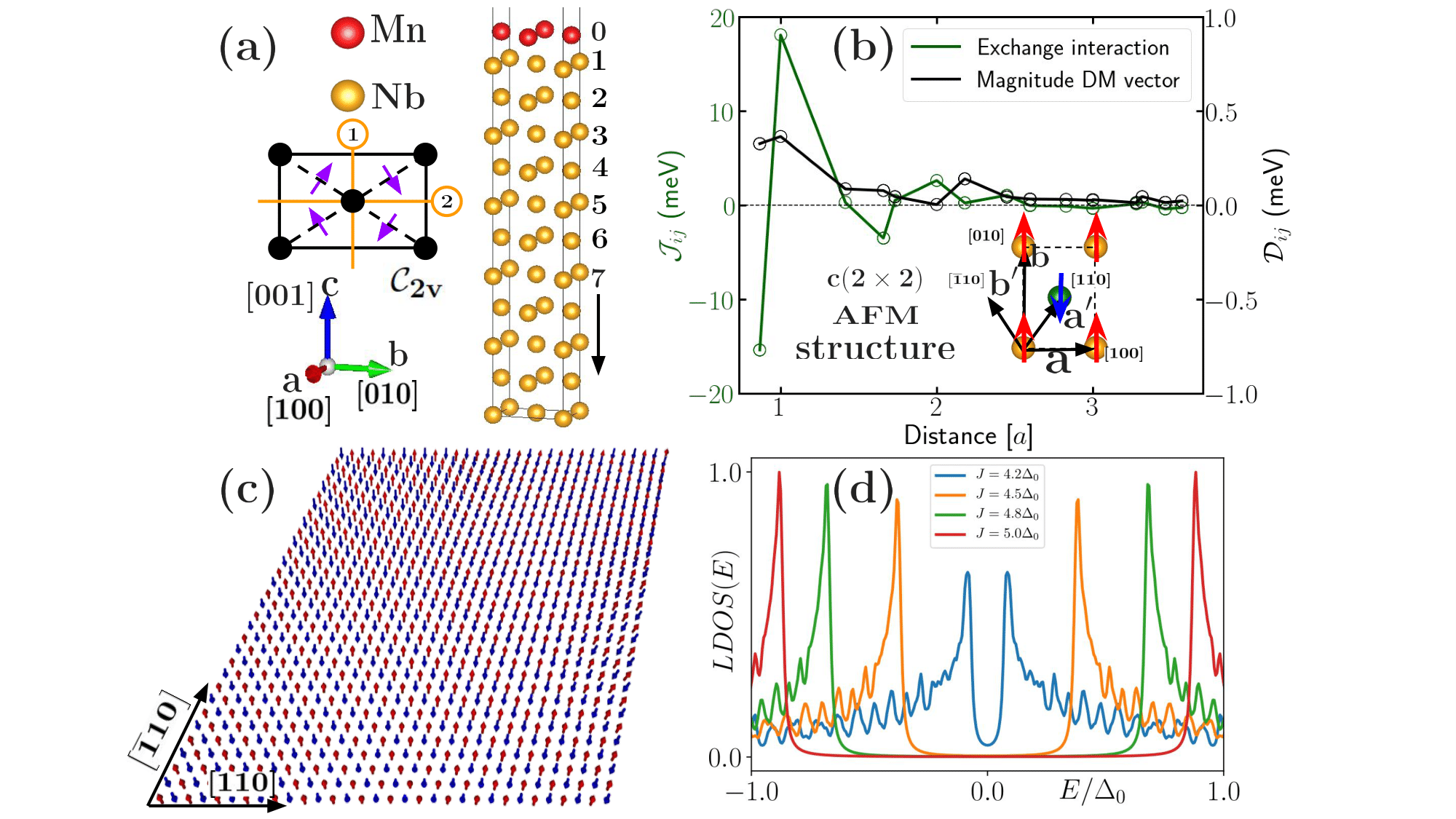
Figure S3: In panel (a), the unit cell of Mn/Nb(110) used for our ab initio calculations. The atoms denoted by red and yellow balls are Mn and Nb atoms, respectively. On the left, the sketch of the rectangular $c(2\times 2)$ surface u.c. has $\mathcal{C}_{2v}$ symmetry with mirror planes ($p$=1, 2) are indicated by yellow lines. The filled black circles represent the surface atoms in the u.c. and the microscopic $\boldsymbol{\mathrm{D}}$ vectors (purple arrows) between NN sites on crystal surface plane are restricted by symmetry to point perpendicular to the bond. Indeed, the calculated vector orientations of all $\boldsymbol{\mathrm{D}}$ vectors in the inset of Fig. 4(a) in the main text follow the $\mathcal{C}_{2v}$ symmetry rules Moriya (1960). In panel (b), we depict the exchange coupling strength, $\mathcal{J}_{ij}$ and DMI strength, $\mathcal{D}_{ij}$ as a function of distance from a reference atom. The interaction parameters, $\mathcal{J}$’s and $\mathcal{D}$’s, till 5^th neighbor cell is also presented in Table 1. We find the expected decay of both $\mathcal{J}$ and $\mathcal{D}$ with distance $|\boldsymbol{\mathrm{R}}_{l}-\boldsymbol{\mathrm{R}}_{0}|$ in units of surface lattice vector $a_{\textrm{opt}}$. In panel (c), we show an AFM spin texture which is found in the Mn layer within the MC simulation. We have used parameters mentioned in (b) and out-of-plane anisotropy, $\mathcal{K}$ = 0.04 $\rm{meV}$ per Mn atom. Panel (d) shows the plot of the local density of states (LDOS) as a function of energy, illustrating the formation of Shiba bands within $\pm\Delta_{0}$ for the $c(2\times 2)$-AFM phase (see the inset of (b)). The exchange field strength $J$ is varied between 4.2$\Delta_{0}$ and 5.0$\Delta_{0}$. We choose $\mu=4.0\Delta_{0},t=\Delta_{0}$.

A domain of size 32$\times$32 has been used for solving Eq. (4) in the main text and the obtained results are summarized in Fig. S3(d), describing the local density of states (LDOS) as a function of energy ($E$). Due to the overlapping of the Yu-Shiba-Rusinov (YSR) in-gap bound states, the Shiba bands are formed within the superconducting gap $\pm\Delta_{0}$. We further vary the coupling constant $J$ between the local magnetization (in the Mn spin texture) and the itinerant spin (free electrons in the SC) to ensure the trivial superconductivity in the system. Precisely, a proximity induced SC sustains in the AFM Mn layer. Based on our results from our model (Eq. (4) in the main text), we can firmly reproduce the experimental findings i.e.,  the coexistence of SC and AFM phases Lo Conte et al. (2022).

S3.2 Role of uniform biaxial surface strain for AFM-SS ground state in Mn/Nb(110) film

Here, we discuss a transition to an AFM-SS state from the $c(2\times 2)$ state in the top Mn layer of Mn/Nb(110) heterostructure by applying an uniform biaxial strain in the 2D film geometry. As the strain changes the in-plane lattice parameters keeping $b$=$\sqrt{a}$ unaltered, the relaxed film is expected to change $\mathcal{J}$’s, $\mathcal{D}$’s and $\mathcal{K}$ value for the magnetic layer. In Table 1, we have presented various quantities calculated within KKR-GF method while the Fig. S4(a) depicts the effect of strains on $\mathcal{J}$’s as a function of distance between Mn atoms. In the second column of the Table 1, the magnetic moment of Mn within KKR-GF calculation is matching well with that of obtained from VASP relaxation calculations. The plot in Fig. S4(a) ensures the strong frustration in $\mathcal{J}$’s even after varying the planar strain from tensile (positive) to compressive (negative). Indeed, the dominating parameters are the Heisenberg exchange parameters and the first two $\mathcal{J}$’s are the strongest in comparison to the rest. In particular, the NN exchange constant (‘$-$ve’ means AFM) is gradually increasing in magnitude with changing strain from tensile to compressive while the trend is opposite in case of NNN (‘$+$ve’ means FM) exchange constant except for $a_{+3.3}$ case, see Table 1.

Interestingly, this strong exchange frustration has adverse effect in the ground state magnetic phase of Mn/Nb(110), where the $c(2\times 2)$-AFM phase remains the lowest energy magnetic configuration under the tensile strain i.e.,  when the 2D surface u.c. is expanded. An AFM-SS state becomes the lowest energy ground state under a small compressive strain of magnitude 1.6 %. It is worth to mention that such AFM-SS ground state is rarely found in film geometry and the number of examples is very limited. Here, this SS state in Fig. S4(c) can be stabilized by the exchange frustration only in the presence of small out-of-plane $\mathcal{K}$. We further increases the compressive strain and the AFM-SS solution is found with a small variation in the period $\lambda_{\textrm{Mn}}$ for strains $-$2.7% and $-$3.7% both. We find that the AFM-SS state exists for a delicate balance between NN AFM and NNN FM $\mathcal{J}$ values. This state is hardly affected by the rest of the isotropic exchange interaction terms. The spin spiral presented in Fig. S4(c) for $-$1.6 % strain has a period of about $\lambda_{\textrm{Mn}}\approx$ 3.52 $\rm nm$ computed using MC simulations. In such cases, the sense of rotation of the SS will have degeneracy which generally breaks in the presence of chiral interactions i.e.,  the DMI. Hence, using the full Hamiltonian in Eq. (S5), we have identified a right-handed cycloidal AFM-SS state, see Fig. S4(b) and also Fig. 4(b) in the main text. Comparing (b) and (c), we find that even relatively weak DMI strength changes the period of the SS to an expected lower value, $\lambda_{\textrm{Mn}}\approx$ 2.35 $\rm nm$, propagating along [010] direction.

The exchange frustration driven AFM-SS is now examined by numerically solving Eq. (4) in the main text. A 32$\times$32 domain as presented in Fig. S4(d) is considered for the spin-lattice model and the corresponding result, particularly the LDOS for the zero-energy ($E=0$) is depicted in Fig. S4(e). The zero-energy states are indeed localized at the edges of the considered magnetic domain while the bulk YSR band is semimetallic. Therefore, this AFM-SS can give rise to MFEM mode (see Fig. S4(e)), even without DMI. Akin to the main text (see inset of Fig. 5(a)), non-dispersive states at the zero-energy is also observed in the eigenvalue spectrum. In general, the antisymmetric DMI term in magnetic films with broken inversion symmetry is the result of an indirect exchange mechanism in the presence of spin-orbit coupling (SOC) present in the substrate elements Dzyaloshinsky (1958); Moriya (1960); Fert and Levy (1980). In many 2D magnetic systems, this plays an important role in stabilizing SS state which otherwise does not appear with the exchange interactions only Lo Conte et al. (2020). This is also true in case of Mn/Nb(110) with optimized lattice constant, see the subsection S3.1. Hence, for Mn/Nb(110) magnetic film, strain is an important controlling parameter to stabilize the AFM-SS state and hence, triggers the TSC phase. Comparing the results presented in the main text Fig. 5(a)-(b) and Fig. S4(e), we have established that the TSC phase transition from a trivial state can occur when the noncollinear spin textures in the form of SS becomes a stable solution in a transition-metal/superconductor (TM/SC) heterostructure even in the absence of DMI, a SOC driven interaction parameter.

Lattice	Magnetic mom.	MCA	DMI magnitude				Isotropic exchange					Ground state
constant in Å	$\mathcal{M}_{\textrm{Mn}}$ in $\mu_{\textrm{B}}$	$\mathcal{K}$ in	in $\rm{meV}$				interaction ($\rm{meV}$)					spin texture
($a_{\textrm{strain}}$)	KKR-GF, (VASP)	${\rm{meV}}$/Mn	$\mathcal{D}_{01}$	$\mathcal{D}_{02}$	$\mathcal{D}_{03}$	$\mathcal{D}_{04}$	$\mathcal{J}_{1}$	$\mathcal{J}_{2}$	$\mathcal{J}_{3}$	$\mathcal{J}_{4}$	$\mathcal{J}_{5}$
3.432 ($a_{+3.3}$)	3.63, (3.51)	0.22	0.53	0.5	0.02	0.05	-12.41	17.96	2.78	-2.6	1.25	AFM
3.366 ($a_{+1.3}$)	3.57, (3.46)	0.17	0.42	0.52	0.04	0.07	-14.44	18.84	1.34	-3.18	0.78	AFM
3.3232 ($a_{0.0}$)	3.56, (3.43)	0.04	0.33	0.37	0.09	0.08	-15.38	18.01	0.03	-3.49	0.5	AFM
3.270 ($a_{-1.6}$)	3.55, (3.43)	0.22	0.28	0.19	0.14	0.07	-16.58	16.16	-0.57	-3.38	0.15	AFM-SS
3.234 ($a_{-2.7}$)	3.53, (3.39)	0.22	0.28	0.11	0.2	0.07	-17.89	15.37	-0.86	-3.26	0.17	AFM-SS
3.200 ($a_{-3.7}$)	3.52, (3.40)	0.29	0.28	0.04	0.27	0.05	-19.61	14.49	-0.67	-2.96	0.3	AFM-SS

List of Supplementary Short Tables 1 The first three columns provide the smallest lattice constants under strain, $\mathcal{M}_{\textrm{Mn}}$ obtained from both KKR-GF and VASP for each Mn atom and single ion MCA constant (all are out-of-plane), respectively. Next, the $\mathcal{D}_{0j}$ and $\mathcal{J}_{i}$ for first few neighboring cells are tabulated. The different lattice constants signify the system is constructed with different uniform biaxial strain values: from top to bottom, tensile 3.3% (a_+3.3), tensile 1.3% (a_+1.3), optimized 0.0% (a_0.0), compressive 1.6% (a_-1.6), compressive 2.7% (a_-2.7), and compressive 3.7% (a_-3.7). The strains are calculated with respect to the optimised lattice constant, $a_{\textrm{opt}}$=3.3232 Å. The last column clearly indicates a transition from a collinear AFM state to a noncollinear AFM-SS state under a small compressive strain.

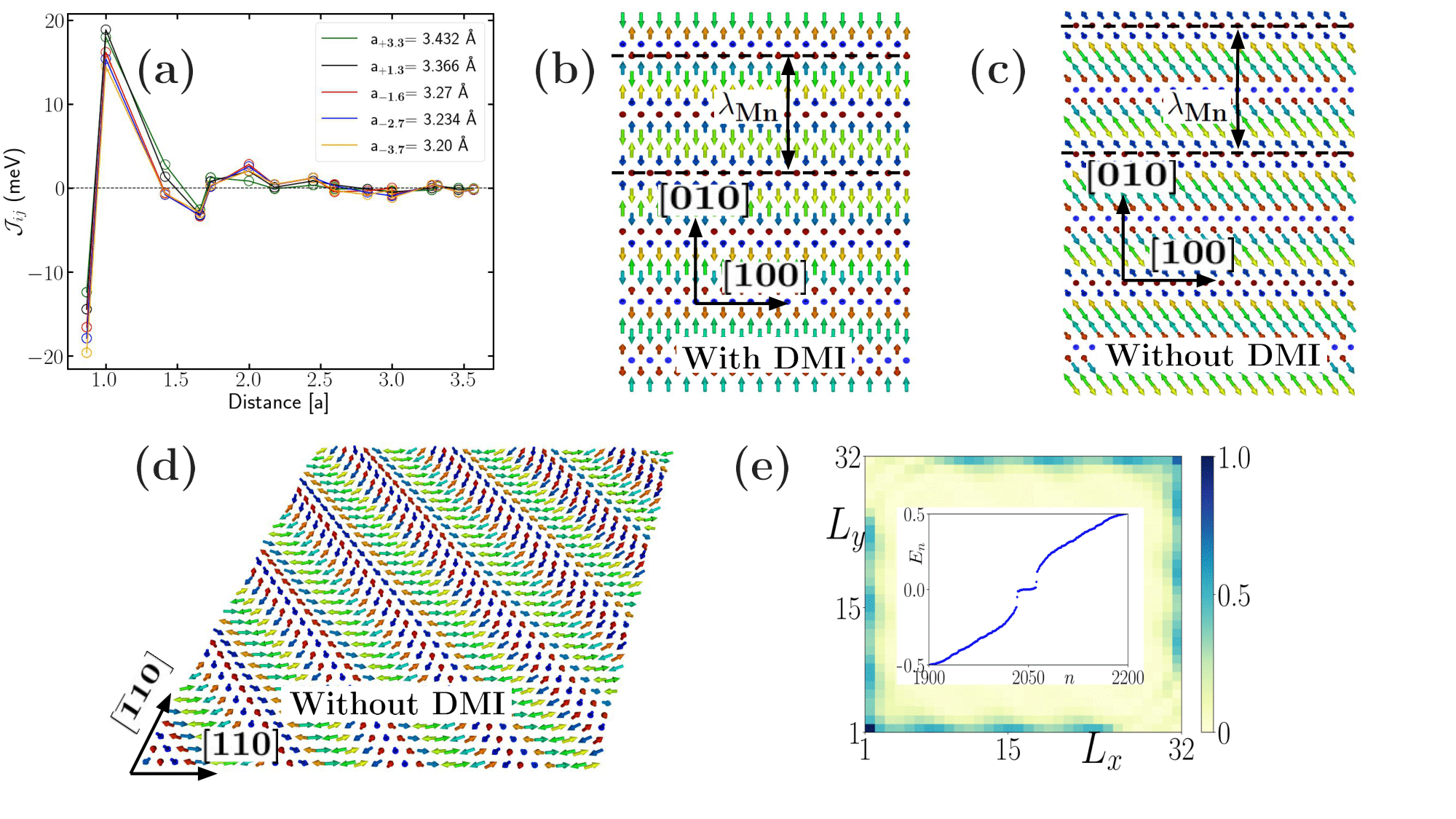
Figure S4: For various strain values, in panel (a) we depict $\mathcal{J}$’s as a function of distance. Spin textures in panels (b) and (c) illustrate the ground state AFM-SS solutions with DMI and without DMI, respectively. The magnitude of the compressive strain is fixed to 1.6. The AFM-SS state becomes an homogeneous right-handed AFM cycloid in the presence of DMI, propagating along [010] direction and the spins are rotated in the $yz$-plane. (d) An AFM-SS domain is constructed from the spin texture shown in panel (c) and hence edges of the domain are [110] and [$\bar{1}$10]. The normalized LDOS corresponding to $E$=0 eigenstate is shown in panel (d) in the $L_{x}\mathchar 45\relax L_{y}$ square plane. The inset depicts the corresponding eigenvalue spectrum $E_{n}$ as a function of the state index $n$. Hence, clearly we obtain TSC phase hosting MFEM in the absence of DMI. Here, we choose $\mu=4.0\Delta_{0},t=\Delta_{0}$ and $J=1.5\Delta_{0}$.

S4 Example of Cr/Nb(110) film: optimized and uniformly planar strained structures

This section deals with another promising prototype candidate, a single layer Cr on Nb(001) substrate, see Fig. S5(a). To the best of our knowledge, no study has been conducted so far on this ultrathin magnetic film sample. The optimized Cr/Mn(001) film exhibits a noncollinear spin texture which is a different type of AFM-SS. Interestingly, the SS ground state is found without any strain. However, we follow the same approach for this system like in Mn/Nb(110) film. In contrast to the Mn/Nb(110) surface u.c., here the surface u.c. possesses square geometry which has $\mathcal{C}_{4v}$ symmetry.

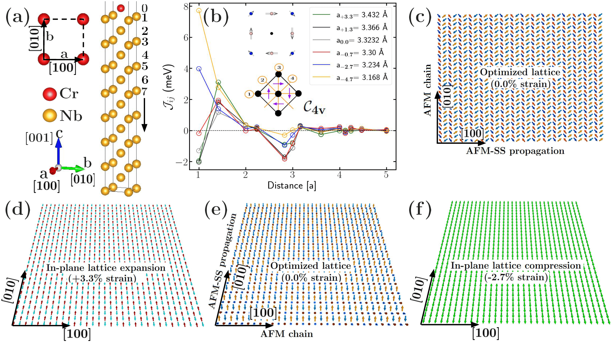
Figure S5: In panel (a), we present the unit cell of Cr/Nb(001). The atoms denoted by red and yellow balls are Cr and Nb atoms, respectively. The usual $\mathcal{J}_{ij}^{\prime}s$ are plotted in panel (b) as a function of distance and the top figure in the inset shows the orientation of NN and NNN DM vectors for the film constructed with optimized lattice constant of Nb. Here, the calculated D vectors are shown on the atoms instead of bonds connection NN and NNN atoms. Below, the sketch of a square surface lattice describing the $\mathcal{C}_{4v}$ symmetry and the mirror planes ($p$=1 to 4) are depicted by yellow lines. The filled black circles represent the surface atoms in the lattice and the microscopic NN $\boldsymbol{\mathrm{D}}$ vectors (purple arrows) on the crystal surface plane respects the symmetry to point perpendicular to the bond. This is indeed matching with the Moriya rules for $\mathcal{C}_{4v}$ symmetric system Moriya (1960). Panel (c) represents the spin texture with interchanging the [100] and [010] directions. In panels (d), (e) and (f), we demonstrate the evolution of the spin textures driven by the strain parameter. They correspond to the in-plane ferromagnetic (with tensile $+3.3$% strain), AFM-SS (with zero strain) and in-plane AFM spin texture (with compressive $-3.7$% strain) respectively.

In Fig. S5(b), we illustrate the behavior of $\mathcal{J}_{ij}$’s under different strain values and the inset describes the orientation of DMI vectors. Note that, following the $\mathcal{C}_{4v}$ symmetry present in the system, the orientation of DMI vectors around a Cr atom are perpendicular to the bond connecting NN and NNN Cr atoms Moriya (1960). As we keep increasing the strain starting from 3.3 % tensile, we observe that the NN exchange interaction changes sign i.e.,  a weak AFM coupling becomes a strong FM coupling, see the exchange interaction part in Table 1. On the other hand, the next dominating exchange constant, the NNN one remains FM for all values of strain. The $\mathcal{D}$ is small here too, owing to the weak SOC strength in Nb. However, compared to Mn/Nb(110) film, the exchange constants are found to be relatively weak. Interestingly, in contrast to Mn/Nb(110), the MCA constants are all in-plane, see the third column in Table 1. A strong variation in $\mathcal{J}$’s under strain makes Cr/Nb(001) film an exciting playground for tailoring magnetism.

Indeed, in Figs. S5(d)-(f), with varying strain, we show that the in-plane AFM ground state for the expanded surface u.c. changes to an in-plane FM ground state under compression. Surprisingly, a noncollinear spin texture (AFM-SS) appears as the ground state with the optimized lattice geometry ($a_{\textrm{opt}}$= 3.3232 Å). This particular AFM-SS in Fig. S5(e) exhibits an AFM chain along [100] direction and spins are rotating in the $yz$-plane. So, the AFM-SS is propagating along [010] direction with the sense of spin rotation left-handed (left-handed cycloid). Here, the period of the spiral is small compared to that of Mn/Nb(110), $\lambda_{\textrm{Cr}}\approx$ 1.33 $\rm{nm}$. This is due to the fast rotation of spins along [010] direction. Here, the interplay between relatively weak, both $\mathcal{J}$’s and $\mathcal{D}$’s stabilizes the SS even in the presence of small in-plane anisotropy. Respecting the $\mathcal{C}_{4v}$ symmetry, the chiral AFM-SS ground state is found to be degenerate in our simulation. The texture in Fig. S5(c) represents another AFM-SS state where the AFM chain along the [010] direction rotates in the $xz$-plane and hence, the propagation direction is [100].

Lattice	Magnetic mom.	MCA	DMI magnitude				Isotropic exchange					Ground state
constant in Å	$\mathcal{M}_{\textrm{Cr}}$ in $\mu_{\textrm{B}}$	$\mathcal{K}$ in	in $\rm{meV}$				interaction ($\rm{meV}$)					spin texture
(a${}_{\textrm{strain}}$)	KKR-GF, (VASP)	$\rm{meV}$/Cr	$\mathcal{D}_{01}$	$\mathcal{D}_{02}$	$\mathcal{D}_{03}$	$\mathcal{D}_{04}$	$\mathcal{J}_{1}$	$\mathcal{J}_{2}$	$\mathcal{J}_{3}$	$\mathcal{J}_{4}$	$\mathcal{J}_{5}$
3.432 (a+3.3)	2.78, (2.83)	-0.40	0.32	0.02	0.02	0.1	-1.96	3.1	0.32	0.07	-0.91	In-plane AFM
3.366 (a+1.3)	2.96, (2.84)	-0.41	0.60	0.29	0.03	0.09	-2.04	1.83	0.34	0.12	-1.72	In-plane AFM
3.3232 (a0.0)	2.69, (2.81)	-0.37	0.85	0.51	0.001	0.05	-1.31	1.16	0.36	0.15	-1.82	AFM-SS
3.300 (a-0.7)	2.69, (2.62)	-0.37	0.89	0.58	0.02	0.05	-0.19	1.93	-0.03	0.08	-1.84	AFM-SS
3.234 (a-2.7)	2.79, (2.55)	-0.28	0.97	0.46	0.15	0.14	3.97	1.39	0.11	0.22	-0.96	In-plane FM
3.168 (a-4.7)	2.38, (2.36)	-0.28	0.7	0.31	0.11	0.15	7.72	2.76	0.33	0.17	-0.31	In-plane FM

List of Supplementary Short Tables 1 The first three columns provide the surface lattice constant under strain, $\mathcal{M}_{\textrm{Cr}}$ obtained from both KKR-GF and VASP in the parenthesis and single ion MCA constant (all are in-plane), respectively. Next, the $\mathcal{D}_{0j}$ and $\mathcal{J}_{i}$ for first few neighboring cells are tabulated. The different lattice constants signify the system is constructed with different uniform biaxial strain values: from top to bottom, tensile 3.3% (a_+3.3), tensile 1.3% (a_+1.3), optimized 0.0% (a_0.0), compressive 1.6% (a_-0.7), compressive 2.7% (a_-2.7), and compressive 4.7% (a_-4.7). The strains are calculated with respect to the optimised lattice constant, $a_{\textrm{opt}}$=3.3232 Å. The last column clearly indicates a transition from an in-plane AFM state to an in-plane FM state via a noncollinear AFM-SS state.

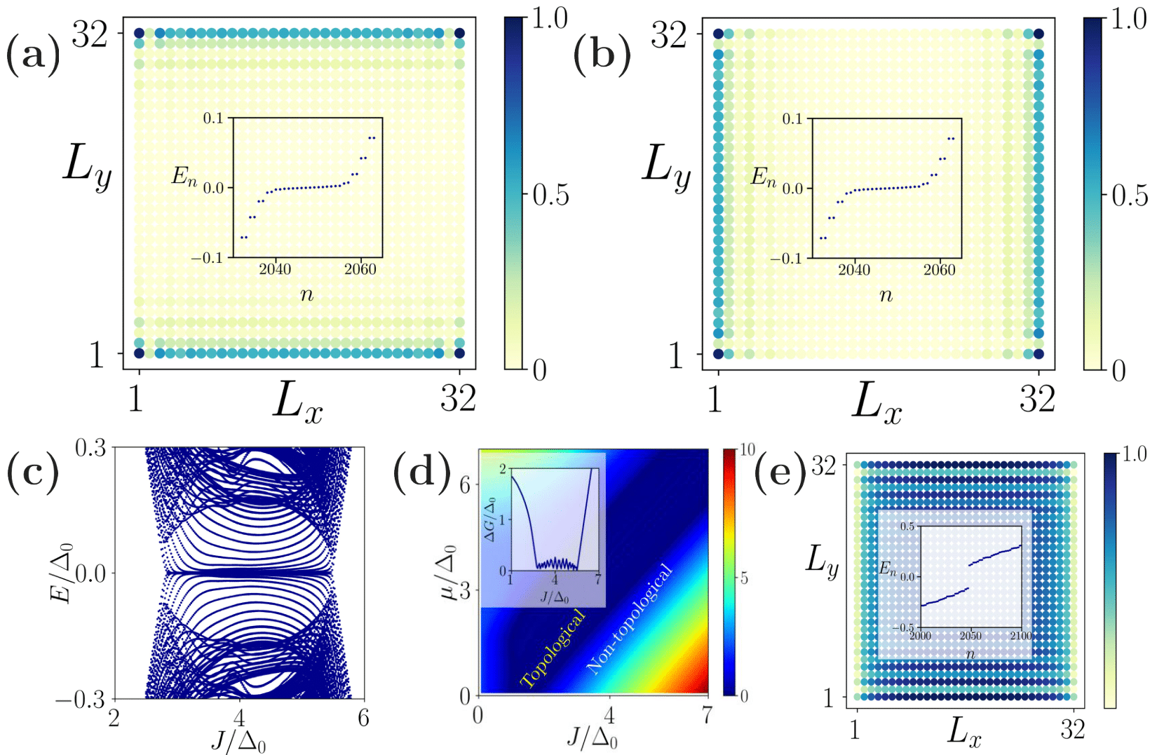
Figure S6: By using a square domain within $L_{x}\mathchar 45\relax L_{y}$ plane, in panels (a) and (b) we depict the normalized LDOS for $E=0$ states at $J=3.5\Delta_{0}$, indicating the MFEM at parallel edges along (100) direction (Fig. S5(c), the corresponding spin texture) and parallel edges along (010) direction (Fig. S5(e), the corresponding spin texture), respectively. Insets show the eigenvalue spectrum $E_{n}$ as a function of the state index $n$. (c) The energy eigenvalues $E$ of the Hamiltonian $H$ (Eq. (4) in the main text) is plotted as a function of the exchange coupling constant $J$ employing open boundary condition. We choose $\mu=4.0\Delta_{0}$ and $\Delta_{0}=t$. (d) The bulk-gap $\Delta G$ profile in the $J\mathchar 45\relax\mu$ plane is shown by employing the periodic boundary condition. The dark (light) blue regime represent the TSC phase (non-TSC phase). In the inset plot, we demonstrate the $\Delta G$ as function of $J$ for a fixed $\mu(=4.0\Delta_{0})$ for more clarity. (e) The trivial phase occurs for $J=5.5\Delta_{0}$ and the eigenvalue spectrum $E_{n}$ as a function of the state index $n$ clearly shows a gap at $E$=0.

Now, based on the solutions obtained from the spin lattice model (Eq. (5) in the main text), Figs. S6(a) and (b) describe the $E=0$ LDOS behavior in the $L_{x}\mathchar 45\relax L_{y}$ plane for domains with spin textures shown in Fig. S5(c) and Fig. S5(e), respectively. Note, here we consider the spin texture in a domain that is the key ingredient in stabilizing the TSC phase. One can clearly find the edges where localization of the $E=0$ state occurs and in both cases the TSC phase is identified. Additionally, the parallel edges where we find the localized non-dispersive MFEM, strongly depend on the nature of the SS. Particularly, in the present case, the degenerate AFM-SS ground states both stabilize the MFEM on the two parallel edges and depending on the propagation direction, edges are orthogonal to each other, compare Fig. S5(c) (corresponding LDOS in Fig. S6(a)) and Fig. S5(e) (corresponding LDOS in Fig. S6(b)). Furthermore, the signature of non-dispersive MFEM is more convincing from the low-lying states (at $E_{n}=0$) in the eigenvalue spectrum, $E_{n}$ as a function of the state index $n$, presented in the insets of Figs. S6(a) and (b). It is worth to mention that in real experiments, such magnetic domain in general possesses both degenerate solutions Ferriani et al. (2008) i.e.,  [100] and [010] propagating SSs together in a single AFM-SS domain and hence, one should expect the MFEM on any edge of a square domain. The calculations are done with exchange coupling strength $J=3.5\Delta_{0}$. On the other hand, in case of $J=5.5\Delta_{0}$ (see Fig. S6(e)), the system becomes topologically trivial. One can identify the disappearance of the MFEM from the LDOS (at $E=0$) distribution in Fig. S6(e) and also, the gapped eigenvalue spectrum in the inset. Thus, the appearance of the MFEM from the real material-based study supports our theoretical proposal, see Fig. 3(c) in the main text.

We depict the energy eigenvalue spectrum ($E/\Delta_{0}$) as a function of $J/\Delta_{0}$ employing open boundary condition in Fig. S6(c). In comparison to that of Mn/Nb(110) (see Fig. 5(c)), the gapless TSC phase hosting MFEM appears in a wider range of $J$, between 3.5$\Delta_{0}$ to 5.3$\Delta_{0}$. To further identify the parameter regime, particularly in the $\mu\mathchar 45\relax J$ plane, in which the MFEM appears, we further investigate the bulk-gap $\Delta G=\lvert E_{2}-E_{1}\rvert$ employing periodic boundary condition. Here, $E_{1}$ and $E_{2}$ represent the two lowest YSR bands. We depict $\Delta G/\Delta_{0}$ in the $J/\Delta_{0}\mathchar 45\relax\mu/\Delta_{0}$ plane in Fig. S6(d), see also Fig. 5(d) in the main text for Mn/Nb(110). Here, the gapless TSC regime is also highlighted by the dark blue strip where $\Delta G\simeq 0$ and the regime outside ($\Delta G>0$) represents the trivial superconducting phase. In the inset of Fig. S6(d), we illustrate the bulk-gap $\Delta G$ as function of $J$ for a fixed value of the chemical potential $\mu$, for further transparent visibility of the TSC regime. The bulk-gap $\Delta G$ vanishes in the topological regime ($\sim$ 3.5$\Delta_{0}$ to 5.3$\Delta_{0}$) and MFEM appears at the boundary (edges of the sample).

S5 YSR/Shiba energy band formation due to the AFM-SS state in the Mn layer on top of Nb (110) surface

In this section of the SM, we discuss about the non-topological Shiba band formed within the energy scale $E=\pm\Delta_{0}$ in the presence of Mn layer as magnetic impurities (AFM-SS) placed on top of an $s$-wave superconductor Nb (110). We obtain the signature of Shiba band when we compute $\rm LDOS$ at the middle of the system. These Shiba bands play the pivotal role during the topological phase transition.

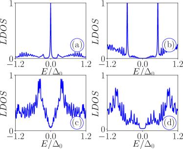
Figure S7: Panels (a), (b) correspond to the behavior of $\rm LDOS$ as a function of $E/\Delta_{0}$ for two different values of exchange coupling strength $J=4.5\Delta_{0}$ and $J=5.0\Delta_{0}$ respectively, when we measure $\rm LDOS$ at the edge of the system. Panels (c), (d) indicate the formation of Shiba bands at the same parameter values when we measure $\rm LDOS$ at the middle of the system.

In Fig. S7(a), we obtain a sharp peak at $E=0$ in the LDOS behavior for $J=4.5\Delta_{0}$. This is a signature of the MFEM (topologically non-trivial) when calculated at the edges of the system. On the other hand, in Fig. S7(c) we depict the corresponding YSR (or simply Shiba) band features in LDOS with the same exchange coupling value $J=4.5\Delta_{0}$, when we compute $\rm LDOS$ at the middle of the system. The semimetallic behavior arising in the LDOS [see Fig. S7 (c)] is the signature of the gaplessness (graphene-like behavior) of the bulk YSR band in the topological regime. This is consistent with the Fig. 2(d) (blue curve) in the main text. On the other hand, Fig. S7(b) and Fig. S7(d) represent $\rm LDOS$ at the edge and middle (YSR/Shiba band) of the system respectively in the non-topological regime (when $J=5.0\Delta_{0}$), where MFEM peak disappears at the edges, see Fig. S7(b). Concomitantly, LDOS in Fig. S7 (d) exhibits a gapped superconductor instead of a semimetallic phase. Similarly, in Fig. S8, panels (a), (b), (c), (d) correspond to the spatial variation of the $\rm{LDOS}$ at finite energy $E=0.1\Delta_{0}$ in the $L_{x}\mathchar 45\relax L_{y}$ plane for four different values of the exchange coupling strength $J=4.0\Delta_{0},4.2\Delta_{0},4.5\Delta_{0},5.0\Delta_{0}$ respectively. One can observe a significant variation of the non-topological Shiba bands for each case due to the presence of the Mn layer as magnetic SS.

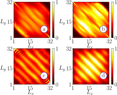
Figure S8: Panels (a), (b), (c), (d) correspond to the vatiation of $\rm LDOS$ at finite energy $E=0.1\Delta_{0}$ in $L_{x}\mathchar 45\relax L_{y}$ plane (highlighting corresponding features of YSR band) with respect to the exchange field strength $J=4.0\Delta_{0},4.2\Delta_{0},4.5\Delta_{0},5.0\Delta_{0}$ respectively.

References

- Kitaev (2001) A Yu Kitaev, “Unpaired majorana fermions in quantum wires,” Physics-Uspekhi 44, 131 (2001).
- Ivanov (2001) D. A. Ivanov, “Non-abelian statistics of half-quantum vortices in -wave superconductors,” Phys. Rev. Lett. 86, 268–271 (2001).
- Nayak et al. (2008) Chetan Nayak, Steven H. Simon, Ady Stern, Michael Freedman, and Sankar Das Sarma, “Non-abelian anyons and topological quantum computation,” Rev. Mod. Phys. 80, 1083–1159 (2008).
- Kitaev (2009) Alexei Kitaev, “Periodic table for topological insulators and superconductors,” AIP Conference Proceedings 1134, 22–30 (2009).
- Qi and Zhang (2011) Xiao-Liang Qi and Shou-Cheng Zhang, “Topological insulators and superconductors,” Rev. Mod. Phys. 83, 1057 (2011).
- Alicea (2012) Jason Alicea, “New directions in the pursuit of majorana fermions in solid state systems,” Reports on Progress in Physics 75, 076501 (2012).
- Leijnse and Flensberg (2012) Martin Leijnse and Karsten Flensberg, “Introduction to topological superconductivity and majorana fermions,” Semiconductor Science and Technology 27, 124003 (2012).
- Beenakker (2013) CWJ Beenakker, “Search for majorana fermions in superconductors,” Annu. Rev. Condens. Matter Phys. 4, 113–136 (2013).
- Aguado (2017) R. Aguado, “Majorana quasiparticles in condensed matter,” Riv. Nuovo Cimento 40, 523 (2017).
- Pientka et al. (2013) Falko Pientka, Leonid I. Glazman, and Felix von Oppen, “Topological superconducting phase in helical shiba chains,” Phys. Rev. B 88, 155420 (2013).
- Nadj-Perge et al. (2013) S. Nadj-Perge, I. K. Drozdov, B. A. Bernevig, and Ali Yazdani, “Proposal for realizing majorana fermions in chains of magnetic atoms on a superconductor,” Phys. Rev. B 88, 020407 (2013).
- Klinovaja et al. (2013) Jelena Klinovaja, Peter Stano, Ali Yazdani, and Daniel Loss, “Topological superconductivity and majorana fermions in rkky systems,” Phys. Rev. Lett. 111, 186805 (2013).
- Braunecker and Simon (2013) Bernd Braunecker and Pascal Simon, “Interplay between classical magnetic moments and superconductivity in quantum one-dimensional conductors: Toward a self-sustained topological majorana phase,” Phys. Rev. Lett. 111, 147202 (2013).
- Vazifeh and Franz (2013) M. M. Vazifeh and M. Franz, “Self-organized topological state with majorana fermions,” Phys. Rev. Lett. 111, 206802 (2013).
- Sau and Demler (2013) Jay D. Sau and Eugene Demler, “Bound states at impurities as a probe of topological superconductivity in nanowires,” Phys. Rev. B 88, 205402 (2013).
- Pientka et al. (2014) Falko Pientka, Leonid I. Glazman, and Felix von Oppen, “Unconventional topological phase transitions in helical shiba chains,” Phys. Rev. B 89, 180505 (2014).
- Pöyhönen et al. (2014) Kim Pöyhönen, Alex Westström, Joel Röntynen, and Teemu Ojanen, “Majorana states in helical shiba chains and ladders,” Phys. Rev. B 89, 115109 (2014).
- Reis et al. (2014) I. Reis, D. J. J. Marchand, and M. Franz, “Self-organized topological state in a magnetic chain on the surface of a superconductor,” Phys. Rev. B 90, 085124 (2014).
- Hu et al. (2015) Wenjian Hu, Richard T. Scalettar, and Rajiv R. P. Singh, “Interplay of magnetic order, pairing, and phase separation in a one-dimensional spin-fermion model,” Phys. Rev. B 92, 115133 (2015).
- Hui et al. (2015) Hoi-Yin Hui, P. M. R. Brydon, Jay D. Sau, S. Tewari, and S. Das Sarma, “Majorana fermions in ferromagnetic chains on the surface of bulk spin-orbit coupled s-wave superconductors,” Scientific Reports 5, 8880 (2015).
- Hoffman et al. (2016) Silas Hoffman, Jelena Klinovaja, and Daniel Loss, “Topological phases of inhomogeneous superconductivity,” Phys. Rev. B 93, 165418 (2016).
- Christensen et al. (2016) Morten H. Christensen, Michael Schecter, Karsten Flensberg, Brian M. Andersen, and Jens Paaske, “Spiral magnetic order and topological superconductivity in a chain of magnetic adatoms on a two-dimensional superconductor,” Phys. Rev. B 94, 144509 (2016).
- Sharma and Tewari (2016) Girish Sharma and Sumanta Tewari, “Yu-shiba-rusinov states and topological superconductivity in ising paired superconductors,” Phys. Rev. B 94, 094515 (2016).
- Andolina and Simon (2017) Gian Marcello Andolina and Pascal Simon, “Topological properties of chains of magnetic impurities on a superconducting substrate: Interplay between the shiba band and ferromagnetic wire limits,” Phys. Rev. B 96, 235411 (2017).
- Theiler et al. (2019) Andreas Theiler, Kristofer Björnson, and Annica M. Black-Schaffer, “Majorana bound state localization and energy oscillations for magnetic impurity chains on conventional superconductors,” Phys. Rev. B 100, 214504 (2019).
- Sticlet and Morari (2019) Doru Sticlet and Cristian Morari, “Topological superconductivity from magnetic impurities on monolayer ,” Phys. Rev. B 100, 075420 (2019).
- Mashkoori and Black-Schaffer (2019) Mahdi Mashkoori and Annica Black-Schaffer, “Majorana bound states in magnetic impurity chains: Effects of -wave pairing,” Phys. Rev. B 99, 024505 (2019).
- Mnard et al. (2019) Gerbold C. Mnard, Christophe Brun, Raphal Leriche, Mircea Trif, Francois Debontridder, Dominique Demaille, Dimitri Roditchev, Pascal Simon, and Tristan Cren, “Yu-shiba-rusinov bound states versus topological edge states in Pb/Si(111),” The European Physical Journal Special Topics 227, 2303–2313 (2019).
- Mashkoori et al. (2020) Mahdi Mashkoori, Saurabh Pradhan, Kristofer Björnson, Jonas Fransson, and Annica M. Black-Schaffer, “Identification of topological superconductivity in magnetic impurity systems using bulk spin polarization,” Phys. Rev. B 102, 104501 (2020).
- Teixeira et al. (2020) Raphael L. R. C. Teixeira, Dushko Kuzmanovski, Annica M. Black-Schaffer, and Luis G. G. V. Dias da Silva, “Enhanced majorana bound states in magnetic chains on superconducting topological insulator edges,” Phys. Rev. B 102, 165312 (2020).
- Rex et al. (2020) Stefan Rex, Igor V. Gornyi, and Alexander D. Mirlin, “Majorana modes in emergent-wire phases of helical and cycloidal magnet-superconductor hybrids,” Phys. Rev. B 102, 224501 (2020).
- Perrin et al. (2021) Vivien Perrin, Marcello Civelli, and Pascal Simon, “Identifying majorana bound states by tunneling shot-noise tomography,” Phys. Rev. B 104, L121406 (2021).
- Shiba (1968) Hiroyuki Shiba, “Classical Spins in Superconductors,” Progress of Theoretical Physics 40, 435–451 (1968).
- Kaladzhyan et al. (2016) V Kaladzhyan, C Bena, and P Simon, “Asymptotic behavior of impurity-induced bound states in low-dimensional topological superconductors,” Journal of Physics: Condensed Matter 28, 485701 (2016).
- Rontynen and Ojanen (2015) Joel Rontynen and Teemu Ojanen, “Topological superconductivity and high chern numbers in 2d ferromagnetic shiba lattices,” Phys. Rev. Lett. 114, 236803 (2015).
- Röntynen and Ojanen (2016) Joel Röntynen and Teemu Ojanen, “Chern mosaic: Topology of chiral superconductivity on ferromagnetic adatom lattices,” Phys. Rev. B 93, 094521 (2016).
- Dai et al. (2022) Ning Dai, Kai Li, Yan-Bin Yang, and Yong Xu, “Topological quantum phase transitions in metallic shiba lattices,” Phys. Rev. B 106, 115409 (2022).
- Ortuzar et al. (2022) Jon Ortuzar, Stefano Trivini, Miguel Alvarado, Mikel Rouco, Javier Zaldivar, Alfredo Levy Yeyati, Jose Ignacio Pascual, and F. Sebastian Bergeret, “Yu-shiba-rusinov states in two-dimensional superconductors with arbitrary fermi contours,” Phys. Rev. B 105, 245403 (2022).
- Ghazaryan et al. (2022) Areg Ghazaryan, Ammar Kirmani, Rafael M. Fernandes, and Pouyan Ghaemi, “Anomalous shiba states in topological iron-based superconductors,” Phys. Rev. B 106, L201107 (2022).
- Schmid et al. (2022) Harald Schmid, Jacob F. Steiner, Katharina J. Franke, and Felix von Oppen, “Quantum yu-shiba-rusinov dimers,” Phys. Rev. B 105, 235406 (2022).
- Chatterjee et al. (2023) Pritam Chatterjee, Saurabh Pradhan, Ashis K. Nandy, and Arijit Saha, “Tailoring the phase transition from topological superconductor to trivial superconductor induced by magnetic textures of a spin chain on a -wave superconductor,” Phys. Rev. B 107, 085423 (2023).
- Yazdani et al. (1997) Ali Yazdani, B. A. Jones, C. P. Lutz, M. F. Crommie, and D. M. Eigler, “Probing the local effects of magnetic impurities on superconductivity,” Science 275, 1767–1770 (1997).
- Yazdani et al. (1999) Ali Yazdani, C. M. Howald, C. P. Lutz, A. Kapitulnik, and D. M. Eigler, “Impurity-induced bound excitations on the surface of ,” Phys. Rev. Lett. 83, 176–179 (1999).
- Yazdani (2015) Ali Yazdani, “Visualizing majorana fermions in a chain of magnetic atoms on a superconductor,” Physica Scripta 2015, 014012 (2015).
- Schneider et al. (2021) Lucas Schneider, Philip Beck, Thore Posske, Daniel Crawford, Eric Mascot, Stephan Rachel, Roland Wiesendanger, and Jens Wiebe, “Topological shiba bands in artificial spin chains on superconductors,” Nature Physics 17, 943–948 (2021).
- Beck et al. (2021) Philip Beck, Lucas Schneider, Levente Rózsa, Krisztián Palotás, András Lászlóffy, László Szunyogh, Jens Wiebe, and Roland Wiesendanger, “Spin-orbit coupling induced splitting of yu-shiba-rusinov states in antiferromagnetic dimers,” Nature Communications 12, 2040 (2021).
- Wang et al. (2021) Dongfei Wang, Jens Wiebe, Ruidan Zhong, Genda Gu, and Roland Wiesendanger, “Spin-polarized yu-shiba-rusinov states in an iron-based superconductor,” Phys. Rev. Lett. 126, 076802 (2021).
- Schneider et al. (2022) Lucas Schneider, Philip Beck, Jannis Neuhaus-Steinmetz, Levente Rózsa, Thore Posske, Jens Wiebe, and Roland Wiesendanger, “Precursors of majorana modes and their length-dependent energy oscillations probed at both ends of atomic shiba chains,” Nature Nanotechnology 17, 384–389 (2022).
- Wang et al. (2017) P. Wang, S. Lin, G. Zhang, and Z. Song, “Topological gapless phase in kitaev model on square lattice,” Scientific Reports 7, 17179 (2017).
- Zhang et al. (2019) K. L. Zhang, P. Wang, and Z. Song, “Majorana flat band edge modes of topological gapless phase in 2d kitaev square lattice,” Scientific Reports 9, 4978 (2019).
- Sedlmayr et al. (2015) N. Sedlmayr, J. M. Aguiar-Hualde, and C. Bena, “Flat majorana bands in two-dimensional lattices with inhomogeneous magnetic fields: Topology and stability,” Phys. Rev. B 91, 115415 (2015).
- Nakosai et al. (2013) Sho Nakosai, Yukio Tanaka, and Naoto Nagaosa, “Two-dimensional -wave superconducting states with magnetic moments on a conventional -wave superconductor,” Phys. Rev. B 88, 180503 (2013).
- Chen and Schnyder (2015) Wei Chen and Andreas P. Schnyder, “Majorana edge states in superconductor-noncollinear magnet interfaces,” Phys. Rev. B 92, 214502 (2015).
- Lo Conte et al. (2022) Roberto Lo Conte, Maciej Bazarnik, Krisztián Palotás, Levente Rózsa, László Szunyogh, André Kubetzka, Kirsten von Bergmann, and Roland Wiesendanger, “Coexistence of antiferromagnetism and superconductivity in Mn/Nb(110),” Phys. Rev. B 105, L100406 (2022).
- Nandy et al. (2016) Ashis Kumar Nandy, Nikolai S. Kiselev, and Stefan Blügel, “Interlayer exchange coupling: A general scheme turning chiral magnets into magnetic multilayers carrying atomic-scale skyrmions,” Phys. Rev. Lett. 116, 177202 (2016).
- Hess et al. (2022) Richard Hess, Henry F. Legg, Daniel Loss, and Jelena Klinovaja, “Prevalence of trivial zero-energy subgap states in nonuniform helical spin chains on the surface of superconductors,” Phys. Rev. B 106, 104503 (2022).
- (57) See the Supplemental Material (SM), which includes Refs Project ; Dzyaloshinsky (1958); Moriya (1960); Müller et al. (2019); Lo Conte et al. (2022); Sedlmayr et al. (2015); Hafner (2008); Kresse and Furthmüller (1996, 1996); Perdew et al. (1996); Kresse and Joubert (1999); Blöchl (1994); Bauer ; Liechtenstein et al. (1987); Zabloudil et al. ; Vosko et al. (1980); Udvardi et al. (2003); Ebert and Mankovsky (2009); van Laarhoven and Aarts (1987); Fert and Levy (1980); Lo Conte et al. (2020); Ferriani et al. (2008), for the details of the topological characterization, methoodology incuding ab initio electronic structure calculations using VASP and KKR-GF and atomistic spin dynamics simulations, results in detail of the strain effect in Mn/Nb(110) example, full details of the new candidate Cr/Nb(001) and the semimetallic behavior detalis.
- Castro Neto et al. (2009) A. H. Castro Neto, F. Guinea, N. M. R. Peres, K. S. Novoselov, and A. K. Geim, “The electronic properties of graphene,” Rev. Mod. Phys. 81, 109–162 (2009).
- Wakabayashi et al. (2010) Katsunori Wakabayashi, Ken ichi Sasaki, Takeshi Nakanishi, and Toshiaki Enoki, “Electronic states of graphene nanoribbons and analytical solutions,” Science and Technology of Advanced Materials 11, 054504 (2010).
- (60) The spectral function has been defined through the zero-temperature Green’s function as =; where =.
- Landau and Binder (2000) P.D. Landau and K. Binder, “A guide to monte carlo methods in statistical physics, cambridge university press, cambridge, england,” (2000).
- (62) “P. j. van laarhoven and e. h. aarts, simulated annealing: Theory and applications, (d. reidel, dordrecht, holland, 1987).” .
- Bera and Mandal (2019) Sandip Bera and Sudhansu S. Mandal, “Theory of the skyrmion, meron, antiskyrmion, and antimeron in chiral magnets,” Phys. Rev. Research 1, 033109 (2019).
- Bera and Mandal (2021) Sandip Bera and Sudhansu S Mandal, “Skyrmions at vanishingly small dzyaloshinskii–moriya interaction or zero magnetic field,” Journal of Physics: Condensed Matter 33, 255801 (2021).
- Müller et al. (2019) Gideon P. Müller, Markus Hoffmann, Constantin Dißelkamp, Daniel Schürhoff, Stefanos Mavros, Moritz Sallermann, Nikolai S. Kiselev, Hannes Jónsson, and Stefan Blügel, “Spirit: Multifunctional framework for atomistic spin simulations,” Phys. Rev. B 99, 224414 (2019).
- Heo et al. (2016) Changhoon Heo, Nikolai S. Kiselev, Ashis Kumar Nandy, Stefan Blügel, and Theo Rasing, “Switching of chiral magnetic skyrmions by picosecond magnetic field pulses via transient topological states,” Scientific Reports 6, 27146 (2016).
- Flovik et al. (2017) Vegard Flovik, Alireza Qaiumzadeh, Ashis K. Nandy, Changhoon Heo, and Theo Rasing, “Generation of single skyrmions by picosecond magnetic field pulses,” Phys. Rev. B 96, 140411 (2017).
- (68) Within generalized gardient apprximation functional, the optimized lattice constant of bulk body-centered-cubic Nb is found to be =3.3232 Å, an excellent agreement with the experimental value of about 3.32 Å Project . The value of is then used to constrauct the optimized film geometry and also strains are measured with respect to .
- Moriya (1960) Tôru Moriya, “Anisotropic superexchange interaction and weak ferromagnetism,” Phys. Rev. 120, 91–98 (1960).
- Bode et al. (2007) M. Bode, M. Heide, K. von Bergmann, P. Ferriani, S. Heinze, G. Bihlmayer, A. Kubetzka, O. Pietzsch, S. Blügel, and R. Wiesendanger, “Chiral magnetic order at surfaces driven by inversion asymmetry,” Nature (London) 447, 190–193 (2007).
- Salemi et al. (2019) Leandro Salemi, Marco Berritta, Ashis K. Nandy, and Peter M. Oppeneer, “Orbitally dominated rashba-edelstein effect in noncentrosymmetric antiferromagnets,” Nature Communications 10, 5381 (2019).
- Hafner (2008) Jürgen Hafner, “Ab-initio simulations of materials using vasp: Density-functional theory and beyond,” Journal of computational chemistry 29, 2044–2078 (2008).
- Kresse and Furthmüller (1996) Georg Kresse and Jürgen Furthmüller, “Efficiency of ab-initio total energy calculations for metals and semiconductors using a plane-wave basis set,” Computational materials science 6, 15–50 (1996).
- Kresse and Furthmüller (1996) G. Kresse and J. Furthmüller, “Efficient iterative schemes for ab initio total-energy calculations using a plane-wave basis set,” Phys. Rev. B 54, 11169–11186 (1996).
- Perdew et al. (1996) John P. Perdew, Kieron Burke, and Matthias Ernzerhof, “Generalized gradient approximation made simple,” Phys. Rev. Lett. 77, 3865–3868 (1996).
- Kresse and Joubert (1999) G. Kresse and D. Joubert, “From ultrasoft pseudopotentials to the projector augmented-wave method,” Phys. Rev. B 59, 1758–1775 (1999).
- Blöchl (1994) P. E. Blöchl, “Projector augmented-wave method,” Phys. Rev. B 50, 17953–17979 (1994).
- (78) The Materials Project, “Materials data on Nb by materials project,” 10.17188/1288516.
- (79) D. S. G. Bauer, “Development of a relativistic full-potential first-principles multiple scattering green function method applied to complex magnetic textures of nano structures at surfaces.” Ph.D. Thesis, RWTH Aachen (2013).
- (80) J. Zabloudil, R. Hammerling, L. Szunyogh, and Weinberger P., “Electron scattering in solid matter: A theoretical and computational treatise (springer, 2005),” .
- Vosko et al. (1980) Seymour H Vosko, Leslie Wilk, and Marwan Nusair, “Accurate spin-dependent electron liquid correlation energies for local spin density calculations: a critical analysis,” Canadian Journal of physics 58, 1200–1211 (1980).
- Liechtenstein et al. (1987) A.I. Liechtenstein, M.I. Katsnelson, V.P. Antropov, and V.A. Gubanov, “Local spin density functional approach to the theory of exchange interactions in ferromagnetic metals and alloys,” Journal of Magnetism and Magnetic Materials 67, 65–74 (1987).
- Udvardi et al. (2003) L. Udvardi, L. Szunyogh, K. Palotás, and P. Weinberger, “First-principles relativistic study of spin waves in thin magnetic films,” Phys. Rev. B 68, 104436 (2003).
- Ebert and Mankovsky (2009) H. Ebert and S. Mankovsky, “Anisotropic exchange coupling in diluted magnetic semiconductors: Ab initio spin-density functional theory,” Phys. Rev. B 79, 045209 (2009).
- van Laarhoven and Aarts (1987) P. J. van Laarhoven and E. H. Aarts, “Simulated annealing: Theory and applications.” (1987), (Dordrecht, Holland: D. Reidel).
- Dzyaloshinsky (1958) I. Dzyaloshinsky, “A thermodynamic theory of “weak” ferromagnetism of antiferromagnetics,” Journal of Physics and Chemistry of Solids 4, 241–255 (1958).
- Fert and Levy (1980) A. Fert and Peter M. Levy, “Role of anisotropic exchange interactions in determining the properties of spin-glasses,” Phys. Rev. Lett. 44, 1538–1541 (1980).
- Lo Conte et al. (2020) Roberto Lo Conte, Ashis K. Nandy, Gong Chen, Andre L. Fernandes Cauduro, Ajanta Maity, Colin Ophus, Zhijie Chen, Alpha T. N’Diaye, Kai Liu, Andreas K. Schmid, and Roland Wiesendanger, “Tuning the properties of zero-field room temperature ferromagnetic skyrmions by interlayer exchange coupling,” Nano Letters 20, 4739–4747 (2020).
- Ferriani et al. (2008) P. Ferriani, K. von Bergmann, E. Y. Vedmedenko, S. Heinze, M. Bode, M. Heide, G. Bihlmayer, S. Blügel, and R. Wiesendanger, “Atomic-scale spin spiral with a unique rotational sense: Mn monolayer on W(001),” Phys. Rev. Lett. 101, 027201 (2008).
Supplemental material for “Topological Superconductivity by Engineering Noncollinear Magnetism in
Magnet/Superconductor Heterostructures: A Realistic Prescription for 2D Kitaev Model”
Pritam Chatterjee
,1,2 Sayan banik
,3 Sandip Bera
,3 Arnob Kumar Ghosh
,1,2 Saurabh Pradhan
,5
Arijit Saha 1,2 and Ashis K. Nandy 3
1Institute of Physics, Sachivalaya Marg, Bhubaneswar-751005, India
2Homi Bhabha National Institute, Training School Complex, Anushakti Nagar, Mumbai 400094, India
3School of Physical Sciences, National Institute of Science Education and Research, An OCC of Homi Bhabha National Institute, Jatni 752050, India
5Lehrstuhl für Theoretische Physik II, Technische Universität Dortmund Otto-Hahn-Str. 4, 44221 Dortmund, Germany