Nonlinear optics from hybrid dispersive orbits

Abstract

In this paper we present an expansion of the technique of characterizing nonlinear optics from off-energy orbits (NOECO) Olsson et al. (2020) to cover harmonic sextupoles in storage rings. The existing NOECO technique has been successfully used to correct the chromatic sextupole errors on the MAX-IV machine, however, it doesn’t account for harmonic sextupoles, which are widely used on many other machines. Through generating vertical dispersion with chromatic skew quadrupoles, a measurable dependency of nonlinear optics on harmonic sextupoles can be observed from hybrid horizontal and vertical dispersive orbits. Proof of concept of our expanded technique was accomplished by simulations and beam measurements on the National Synchrotron Light Source II (NSLS-II) storage ring.

I introduction

Characterizing the nonlinear optics of storage rings is becoming more essential with the introduction of higher order multipole magnets in accelerator design. Errors from the higher order multipoles have been observed to degrade machine performance, such as reduction of dynamic aperture, energy acceptance, etc. Some efforts have been made to identify the nonlinear multipole errors by measuring distorted resonance driving terms Franchi et al. (2014), which requires a complicated Hamiltonian dynamics analysis. A more practical technique for measuring the nonlinear optics from off-energy closed orbits (NOECO) was reported and demonstrated on the MAX-IV ring Olsson et al. (2020). Significant improvements on its dynamic aperture and beam lifetime were observed after correcting sextupole errors. Desired results were obtained while testing the NOECO technique on the ESRF-EBS ring as well Liuzzo et al. (2022). However, the dependency of nonlinear optics on off-energy orbits is only measurable for chromatic sextupoles. The horizontal dispersion seen by chromatic sextupoles are usually quite large, as to effectively correct the chromaticity. This technique, however, doesn’t apply to harmonic sextupoles, which do not see the first order linear dispersion. Harmonic sextupoles are used in almost every third-generation light source ring, and some fourth-generation diffraction-limited machines, such as the ALS-U ring Steier et al. (2019). They are even being used in the design of a future electron-ion collider ring Cai et al. (2022). As such, an expansion of the existing NOECO technique to correct for the harmonic sextupoles would be useful due to their common, integral use in current and future accelerator design. In the National Synchrotron Light Source II (NSLS-II) ring Dierker (2007), the number of harmonic sextupoles are greater than the number of chromatic sextupoles (180:90). Therefore, correcting harmonic sextupole errors is important for improving machine performance due to their greater influence. In this paper, we outline our expansion on the capabilities of existing sextupole correction techniques to accommodate for the harmonic sextupoles.

A straightforward method for calibrating harmonic sextupoles for correction would be to temporarily convert them to chromatic ones. This could be achieved by tuning the quadrupoles inside achromats to generate a commensurate amount of dispersion at the locations of harmonic sextupoles Olsson . However, this method would require a significant modification of the original linear lattice. Implementations during online measurements, such as updating the nonlinear optics dependency for different leaked dispersion bumps would also be complicated. Another method would be to generate local orbit bumps, calibrated through the sextupoles, and then measuring the optics distortion with different bump parameters. This method would not only require sufficient beam position monitors (BPMs) that neighbor the sextupoles, but would also be complicated to implement. In real-world applications, it is time-consuming to form perfectly closed local bumps with orbit correctors, and then to update the optics dependence on these bump settings Choi . While the above methods would be capable of achieving the desired outcome, they are not practical when considering the limitations of routine operations of user facilities.

When a sextupole sees vertical dispersion, the nonlinear optics of the off-energy orbits will also depend on its gradient $K_{2}=\frac{1}{(B\rho)_{0}}\frac{\partial^{2}B_{y}}{\partial x^{2}}$, normalized with the beam rigidity $(B\rho)_{0}$. A vertical dispersive wave can be generated through chromatic skew quadrupoles. In most light source rings, skew quadrupoles are widely equipped to control the residual vertical dispersion and linear coupling. Usually, a considerable amount of vertical dispersion can be generated, but only introduces weak coupling when the Betatron tune has sufficiently diverged from the linear difference/sum resonance. Thus, the nonlinear off-energy optics depends on not only chromatic sextupoles, but also on the original harmonic ones. In other words, horizontal harmonic sextupoles are converted into vertical chromatic ones, which makes their calibration and correction possible on hybrid dispersive orbits. In our studies, the NSLS-II ring double-bend achromat lattice was used to demonstrate these expanded capabilities.

The remainder of this paper is outlined as follows: Sect. II introduces the principle of the technique in conjunction with the NSLS-II lattice. In Sect. III we demonstrate our technique with some simulations. Some beam measurements to calibrate both the chromatic and harmonic sextupole errors are given in Sect. IV, with the caveat that no real sextupole correction can be implemented at this time due to their in-series power supplies. Sect. V discusses the hardware requirements necessary to apply this technique. A brief summary is given in Sect. VI.

II Nonlinear optics on hybrid dispersive orbit

Chromatic skew quadrupoles (located at horizontally dispersive sections) can couple the dispersion function between the horizontal and vertical planes. This property is widely used to minimize the vertical beam size in most light source rings. At the NSLS-II ring, each odd-numbered cell is equipped with one $0.2\;m$ long chromatic skew quadrupole (see Fig. 1). Their maximum gradients are $g_{1}=0.35\;T\cdot m^{-1}$, which is limited by the capacity of their power supplies. Assuming we can double their gradients to $g_{1}=0.70\;T\cdot m^{-1}$, a vertical dispersion wave with a $\sim 0.1\;m$ amplitude can be generated. The necessity for a double gradient will be discussed in Sect. V. Although these gradients are twice as large as the maximum output of their power supplies, they are still quite weak compared to other operational quadrupoles with a maximum gradient of $g_{1,max}=22\;T\cdot m^{-1}$. Under these conditions, the exact coupled optics computed with the Ripken parameterization Borchardt et al. (1988); Willeke and Ripken (1989) indicates that the linear optics remain weakly coupled. In Fig. 1, the non-dominated functions $\beta_{1,y}$ and $\beta_{2,x}$ (dashed lines) are observed as very close to zero, while the dominated $\beta_{1,x}$ and $\beta_{2,y}$ (solid lines) are almost the same as in the uncoupled case. The skew quadrupoles also cause a small amount of horizontal dispersion to be leaked into the straight sections. Although such small residual dispersion could not be solely used to measure the off-energy nonlinear optics, its effect is accounted for in our method because the exact parameterization has been used. In short, when the machine tune is configured to avoid linear coupling resonances, chromatic skew quadrupoles can generate a considerable amount of vertical dispersion, but only introduce relatively small linear coupling. The newly generated vertical dispersion seen by the original harmonic sextupoles can make the nonlinear optics on off-energy orbits (as illustrated in Fig. 2) dependent on their gradients. Therefore, this dependence can be utilized for their calibration and correction.

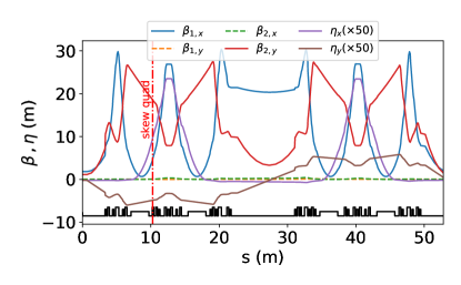
Figure 1: Exact Ripken Twiss functions for a supercell at NSLS-II when a vertical dispersion wave is generated with chromatic skew quadrupoles (with a normalized gradient $K_{1,s}=\frac{1}{(B\rho)_{0}}\frac{\partial B_{y}}{\partial x}=0.070\;m^{-2}$). The location of the skew quadrupole is marked with a red vertical dash-dot line. Two non-dominated $\beta$-functions (dashed lines) indicate that this optics configuration remains weakly coupled.

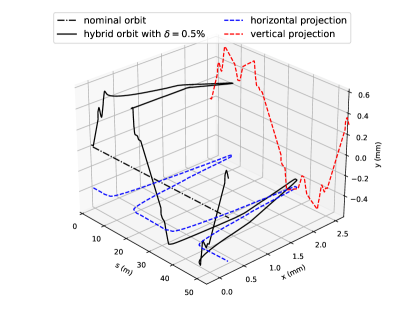
Figure 2: Three-dimensional view of the hybrid dispersive orbit with $\delta=0.5\%$ for one NSLS-II supercell.

When horizontal dispersion is seen by sextupoles in an uncoupled linear optics configuration, the dependence of the $\beta$-function on the beam energy deviation, $\delta=\frac{\Delta P}{P}$, and the normalized sextupole gradient, $K_{2}$, can be formulated Wiedemann (2015). When both horizontal and vertical dispersion can be seen by sextupoles in a weakly coupled optics configuration, no such simple formulae are available. However, it can be numerically computed with the two following methods. Method 1: First, for a given energy offset $\delta$ and skew quadrupole settings $K_{1,s}$, a hybrid dispersive closed orbit can be obtained with iterative tracking. This hybrid dispersive orbit now has both the horizontal and vertical offsets. Then a one-turn matrix $R$ can be obtained along the dispersive orbit with a truncated power series algorithm technique Berz (1988). From the linear components, four coupled Ripken Twiss functions can then be extracted and propagated around the whole ring. By slightly tweaking the settings of an arbitrary sextupole with a $dK_{2}$, and repeating the above procedure, the dependence of $\frac{d\beta}{d\delta}$ on $K_{2}$ can be determined. Method 2: A direct particle tracking can be implemented with the same lattice setting as described in the previous method. When the initial particle coordinates are confined within the linear regime, the linear one-turn matrix $R$ can also be fitted from turn-by-turn trajectories. Then the Ripken Twiss functions can be parameterized. After comparing the results for one sextupole using these two methods, which were yielded respectively with the mad-x PTC analysis Schmidt (2005) and the particle trajectory tracking with the code elegant Borland (2000), the results of both methods were consistent 3.

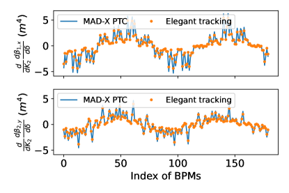
Figure 3: Comparison of the optics dependence on one harmonic sextupole computed with different methods. Top: the response vector in the horizontal plane. Bottom: the response vector in the vertical plane

For demonstration purposes, we choose a harmonic sextupole “SH3” and a chromatic sextupole “SM1” to compute their linear dependence on the off-energy optics, i.e., the so-called response vectors, as seen below. Only two dominated optics functions $\frac{d\beta_{1,x}}{d\delta}$ and $\frac{d\beta_{2,y}}{d\delta}$ observed at their corresponding BPMs were computed. If no skew quadrupoles are used to excite the beam, the optics functions degenerate to the uncoupled $\beta_{x}$ and $\beta_{y}$. The response vectors computed with and without the vertical dispersion are compared in Fig. 4. With horizontal-only dispersive orbits, the dependence of off-energy optics on “SH3(N)” is not measurable in both the horizontal and vertical planes. On the hybrid dispersive orbits, a measurable dependence on “SH3(Y)” can be observed. Note that, for both cases, the dependence of the chromatic “SM1(Y/N)” is always measurable because it sees a large horizontal dispersion. In the meantime, the dependencies are quite similar since the optics are only slightly altered.

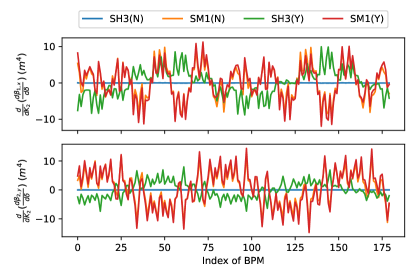
Figure 4: Comparison of the off-energy optics dependence on a chromatic sextupole “SM1” and a harmonic sextupole “SH3”. On horizontal-only dispersive orbits, the optics dependence on the harmonic sextupole (labeled as “SH3(N)”) is too small to measure. On hybrid dispersive orbits, a measurable dependence (labeled as “SH3(Y)”) is observed.

In principle, chromatic and harmonic sextupole errors can be calibrated simultaneously with a sufficiently large vertical dispersion. However, chromatic sextupoles usually have stronger responses than harmonic ones, particularly when the dispersion in the vertical plane is coupled from the horizontal plane. Therefore, for practical purposes, we can uncouple the chromatic and harmonic sextupole correction via a two-stage correction. Stage-1: correcting chromatic sextupoles first with the existing technique Olsson et al. (2020). Stage-2: generating a vertical dispersion wave, then calibrating harmonic sextupoles from hybrid dispersive orbits. In this paper, we only focus on the $2^{nd}$ stage because the $1^{st}$ stage has already been well studied with the linear optics from closed orbits (LOCO) algorithm Safranek (1997) in the ref. Olsson et al. (2020).

The $\beta$-functions and phase advances can be measured directly from turn-by-turn data using the harmonic analysis Borer et al. (1992), or the numerical analysis of fundamental frequencies (NAFF) algorithm Laskar et al. (1992); Zisopoulos et al. (2013). Therefore, instead of the LOCO algorithm, the dependence of $\frac{d\beta}{d\delta}$ on the harmonic sextupole settings $dK_{2}$, which were deliberately mis-set, was used in our simulations. Given a vertical dispersion wave pattern as shown in Fig. 1, the response matrices of $\frac{d\beta_{(1,x),(2,y)}}{d\delta}$ dependence on 180 harmonic sextupoles were computed with the lattice model and illustrated in Fig. 5. Here, we only used two dominated $\beta_{(1,x),(2,y)}$-functions, and the other two non-dominated ones, $\beta_{(1,y),(2,x)}$, were ignored because they are too small to measure accurately.

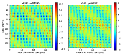
Figure 5: Given a hybrid dispersion wave in Fig. 1, the harmonic sextupole response matrices (RM) observed at the BPMs are obtained by computing the deviation of $\frac{d\beta}{d\delta}$ while slightly changing each individual harmonic sextupole from its nominal setting. Left: the dominated $\beta_{1,x}$ function’s RM in the horizontal plane. Right: the dominated $\beta_{2,y}$ function’s RM in the vertical plane.

III Simulations

Below we simulated two specific cases to study the performance of our expanded sextupole correction technique.

III.1 Case 1: two individual isolated errors

First, we studied a case in which two isolated (far apart from each other) sextupoles errors $\Delta K_{2}=+1.5,\;-1m^{-3}$ were added onto the $32^{th},\;154^{th}$ harmonic sextupoles. The distortions of $\Delta\frac{d\beta}{d\delta}$ observed at the BPMs are shown with the dashed lines in Fig. 6. The needed corrections $\Delta K_{2}$ were obtained by solving the following linear regression problem with the response matrices computed in the previous section,

$$\Delta\frac{d\beta}{d\delta}\approx M_{x,y}\Delta K_{2},$$ (1)

here, $M_{x,y}$ represents a vertically stacked matrix with the horizontal and vertical response matrices.

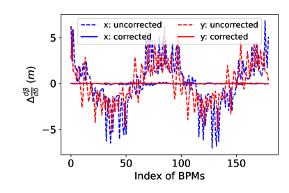
Figure 6: Comparison of nonlinear optics distortions before and after correction in the presence of two isolated sextupole errors. The dashed lines are the uncorrected distortions, and the solid lines represent the corrected ones.

The correction scheme obtained with Eq. (1) for 180 harmonic sextupoles is shown in Fig. 7. Due to the high degeneracy among the neighboring sextupoles, the scheme doesn’t reproduce the original error distributions. Instead, they spread to their neighbors. Nevertheless, the errors were localized, and after applying the correction scheme, the nonlinear optics were recovered as illustrated in Fig. 6.

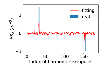
Figure 7: Correction scheme for two isolated sextupole errors obtained by the linear regression algorithm. Despite high degeneracy among sextupoles, two error sources are precisely localized.

III.2 Case 2: normally distributed errors

In this case, random distributed errors on all 180 harmonic sextupoles are introduced and the distortion of off-energy optics are computed. Then the same correction procedure is employed. For comparison, the optics distortions before and after correction, and the real error distributions and computed correction scheme are illustrated in Fig. 8 and Fig. 9), respectively.

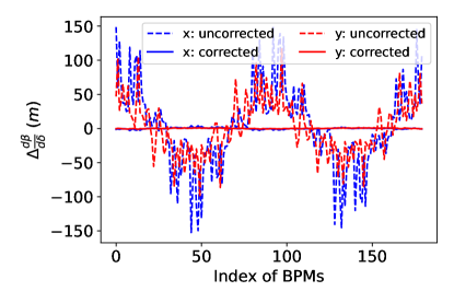
Figure 8: Distortions of the nonlinear optics with 180 randomly added errors. The dashed lines are uncorrected distortions, and the solid lines represent the distortions after correction.

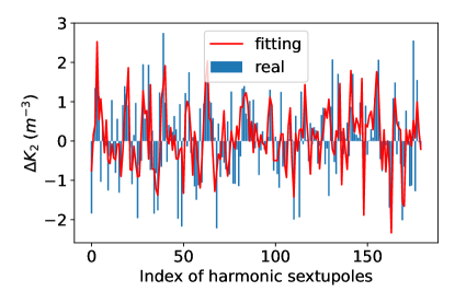
Figure 9: Comparison of the added errors (labeled as “real”) on 180 harmonic sextupoles and the obtained correction scheme (shown with red lines labeled as “fitting”).

In both cases, as seen in Fig. 7 and 9, the obtained correction schemes only approximately follow the real errors that were added in advance. This is due to the strong degeneracy that exists among sextupoles in the NSLS-II lattice. Minor imperfections of the BPMs, and other errors can also result in some degeneracy. However, the distortion of nonlinear optics can still be well corrected in Fig. 6 and 8. It is also worth mentioning that the dependence of nonlinear optics on sextupoles is not purely linear, therefore, an iterative correction might be necessary in online measurements.

III.3 Improvement on dynamic aperture degradation

As observed in the previous simulations, strong degeneracy among sextupoles prevents reproducing the real error distributions accurately. It is because, on the NSLS-II ring, every three harmonic sextupoles on the same girder are closely assembled. In our case, what is actually corrected is the distorted nonlinear optics dependence on beam energy deviations seen by the BPMs. The correction scheme based on the BPM observations, therefore, might only be able to recover the optics distortion rather than the dynamic aperture. To illustrate this, the dynamic apertures of the ideal machine, and uncorrected/corrected nonlinear lattices for the $2^{nd}$ simulation were computed for comparison (Fig. 10). Although the degraded dynamic aperture due to sextupole errors could not be fully recovered through the correction scheme, a significant improvement was achieved. Such improvement is the main purpose of calibrating and correcting the distorted nonlinear optics. If we could distinguish between the degeneracy among the sextupoles, further improvement could be made. This topic is slightly beyond the scope of this paper, however, but worth more study.

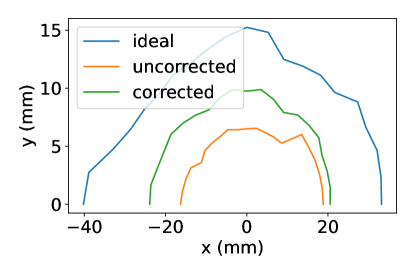
Figure 10: Comparison of the dynamic apertures for the ideal machine, and uncorrected/corrected nonlinear lattices. Although the degraded dynamic aperture (yellow line) could not be well recovered to that of the ideal machine (blue line), significant improvement (green line) was achieved, through correcting the distorted nonlinear optics.

IV Measurements

IV.1 Two-stage measurements

A two-stage proof-of-principle through online calibration of sextupole errors was implemented at the NSLS-II storage ring. As the sextupoles are powered in series, the sextupoles lack individual configurability. Therefore, no actual nonlinear optics correction can be implemented with these limitations. For stage-1, we calibrated 90 chromatic sextupoles with existing techniques. First, spurious vertical dispersion was minimized using 15 chromatic skew quadrupoles, and the global linear coupling was well corrected with another 15 non-dispersive skew quadrupoles. The $\frac{d\beta}{d\delta}$ seen by the BPMs were measured from horizontal dispersive orbits through varying the beam energies. By comparing the measured nonlinear optics against the design model, the chromatic sextupole errors (red bars in Fig. 11) were obtained using the model response matrices, and then incorporated into the lattice model. The updated model would be used as the reference for the stage-2 calibration.

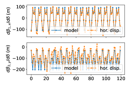
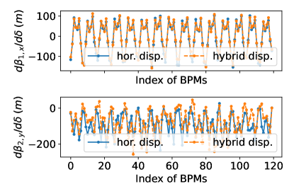
Figure 11: Measured off-energy optics at two stages. Top: off-energy optics based on the ideal model and online measurements from horizontal dispersive orbits which can be used to calibrate chromatic sextupoles. Bottom: online measurements of off-energy optics from horizontal and hybrid dispersive orbits, which can be used to calibrate harmonic sextupoles.

For stage-2, a vertical dispersion wave was generated with 15 dispersive skew quadrupoles to their maximum capacity. Based on the measured dispersion, the 15 skew quadrupole settings and the vertical dispersion at the BPMs were reproduced with the lattice model as illustrated in Fig. 12. To achieve greater accuracy, a large amplitude vertical dispersion wave is preferred. However, it is limited by the capacity of the skew quadrupole power supply. Under the current configuration, $\sim 0.05\;m$ is the maximum amplitude that can be generated. The $\frac{d\beta}{d\delta}$ seen by the BPMs were re-measured, but from hybrid dispersive orbits this time. With the updated lattice model (incorporated with skew quadrupoles and chromatic sextupole errors) as the new reference, 180 harmonic sextupole errors were obtained (blue bars in Fig. 11.

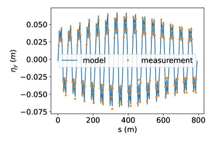
Figure 12: Measured vertical dispersion seen by the BPMs, and its reproduction with the lattice model.

The off-energy optics ($\beta$-functions) were measured with different RF frequencies $f_{0}+\Delta f$, i.e., different energy $\delta=-\frac{1}{\alpha_{c}}\frac{\Delta f}{f_{0}}$, with $\alpha_{c}$ the momentum compaction factor, and $f_{0}$ the nominal RF oscillator frequency for on-momentum electrons. Using Eq. (1), the sextupole errors were calibrated as illustrated in Fig. 13.

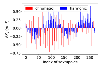
Figure 13: Calibrated sextupole errors from the two-stage measurements. The chromatic sextupoles marked with red bars are from the first stage, while the harmonic ones (blue bars) are from the second stage.

IV.2 Validation of stage-2 measurement

Skew quadrupoles used as correctors are usually operated with dual polarity power supplies. By flipping skew quadrupole polarities, hybrid dispersive orbits are also flipped in the vertical plane. In Appendix Appendix: flipped dispersive orbit in the vertical plane, we prove that the off-energy optics dependence on sextupoles in the flipped orbit remains unchanged when the Ripken parameterization is used. Therefore, we can repeat the stage-2 measurement on the flipped vertical dispersive orbits as a validation. In Fig. 14, two out-of-phase dispersion waves were obtained by flipping all skew quadrupole outputs $K_{1}$ from $-0.035\;m^{-2}$ to $0.035\;m^{-2}$. On the flipped vertical dispersive orbits, stage-2 measurements of off-energy optics changed with respect to stage-1, were repeated as illustrated in Fig. 15. A similar pattern can be recognized in two independently measured optics distortions. This indicates that the dependence of off-energy optics on harmonic sextupoles is measurable on the hybrid dispersive orbit, although the precision is limited by the low capacity of skew quadrupole power supplies.

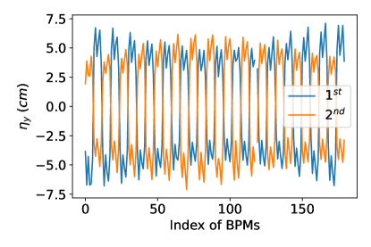
Figure 14: Out-of-phase vertical dispersion waves were generated with flipped skew quadrupole polarities.

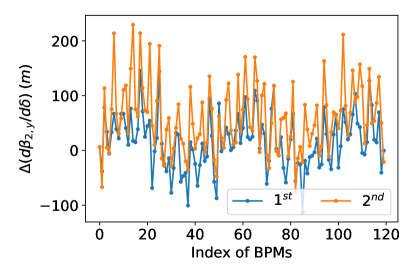
Figure 15: Similar off-energy optics distortions were observed when the hybrid dispersive orbit was flipped in the vertical plane.

V Requirements on power supplies of magnets

In this section, we estimate the requirements of the power supplies for the skew quadrupoles and sextupoles to make this calibration and correction practical, specifically on the NSLS-II ring. First, sextupoles need to be powered independently, or equipped with back-leg windings to allow individual corrections. Second, the skew quadrupoles that generate the vertical dispersion wave should be sufficiently strong for better resolution. Next, we use the NSLS-II lattice to estimate the required skew quadrupole strengths.

The measurement accuracy of $\beta$-functions using turn-by-turn data was found at the level of about $0.03\;m$ on the NSLS-II storage ring. If we adjust the RF frequency by $\pm 1,000\;Hz$, the corresponding energy deviation is $\Delta\delta=-\frac{1}{\alpha_{c}}\frac{\Delta f}{f_{0}}\approx 1.0\%$ with $\alpha_{c}$ momentum compaction factor. To resolve a single harmonic sextupole error to the level of 1 unit $\Delta K_{2}=1\;m^{-3}$, the magnitude of $\frac{d}{dK_{2}}\frac{d\beta}{d\delta}$ needs to be greater than $3\;m^{4}$. To generate such a strong dependence, the amplitude of the vertical dispersion wave is required to be greater than $0.1\;m$. In order to couple $0.1\;m$ dispersion to the vertical plane, $K_{1,sm}\geq 0.07\;m^{-2}$ must be applied to all 15 skew quadrupoles. Therefore, strong skew quadrupoles were chosen to identify two isolated errors in our simulations. Although a $\frac{\partial B_{x}}{\partial x}=0.70\;T\cdot m^{-1}$ quadrupolar gradient is still quite weak, it already exceeds the capacity of our skew quadrupole power supplies $g_{2,max}=0.35\;T\cdot m^{-1}$. In other words, stronger skew quadrupoles are needed to generate larger vertical dispersion for better resolution. As all 270 sextupoles have some associated errors, the accumulated magnitude of $\Delta\frac{d\beta}{d\delta}$ are at the level of 100-200 meters, which allows us to calibrate the approximate error distribution in Sect. IV.

The above estimation doesn’t consider even higher orders of nonlinear optics from off-energy orbits. Once the higher order nonlinearities $\frac{d^{n}\beta}{d\delta^{n}}$ with $n\geq 2$ appear, we couldn’t improve the measurement accuracy by increasing beam energy off-sets. On the other hand, increasing skew quadrupole strengths to generate higher vertical dispersive orbits can significantly improve the sensitivity of off-energy optics to sextupole settings without introducing too much nonlinearity. Therefore, having sufficiently strong skew quadrupoles should be considered a necessary condition for this technique.

VI Summary

We expanded the capability of the technique for measuring nonlinear optics distortions from off-energy orbits to account for the harmonic sextupole contribution. Using hybrid dispersive off-energy nonlinear optics, the errors of the harmonic sextupoles can be measured. The corresponding correction can be more effectively implemented if they are independently configurable. A practical benefit of our expanded method is that a considerable amount of vertical dispersion can be generated with weak skew quadrupoles. Meanwhile, because the original lattice is already weakly coupled, its optics properties can still be well maintained. Thus far, only sextupole calibration was considered in our studies, and higher order nonlinear magnets, such as octupoles, we have not yet investigated. This technique might be applicable if their contributions were sufficiently strong.

Appendix: flipped dispersive orbit in the vertical plane

The hybrid dispersive orbit can be flipped only in the vertical plane by changing the skew quadrupole polarities. Usually skew quadrupoles used for the correction purposes are operated with dual polarity power supplies. In this appendix, we prove that an exact flipping of the vertical dispersive orbit doesn’t change the dependence of off-energy optics on sextupoles which can be used to validate online measurements.

VI.1 Transfer matrix with single skew quadrupole

The $4\times 4$ transfer matrix of a normal quadrupole reads as

$$T_{n}=\left[\begin{matrix}T_{x}&\mathbf{0}\\ \mathbf{0}&T_{y}\end{matrix}\right]$$ (2)

with two $2\times 2$ zero blocks $\mathbf{0}$ as its off-diagonal matrices.

After rotating it by $\frac{\pi}{4}$ around the longitudinal axis, it becomes a skew with a transfer matrix

$$T_{s}=R_{z}\left(\frac{\pi}{4}\right)T_{n}R_{z}\left(-\frac{\pi}{4}\right)=\left[\begin{matrix}\frac{T_{x}+T_{y}}{2}&\frac{-T_{x}+T_{y}}{2}\\ \frac{-T_{x}+T_{y}}{2}&\frac{T_{x}+T_{y}}{2}\end{matrix}\right]$$ (3)

where $R_{z}\left(\theta\right)$ represents the transfer matrix of a pure rotation with an angle of $\theta$.

Assuming there is only one skew quadrupole inside a periodic lattice cell with the layout “normal section 1 – skew quad – normal section 2”, the transfer matrix of the whole section is

$$M_{t}=\left[\begin{matrix}M_{x,2}&\mathbf{0}\\ \mathbf{0}&M_{y,2}\end{matrix}\right]T_{s}\left[\begin{matrix}M_{x,1}&\mathbf{0}\\ \mathbf{0}&M_{y,1}\end{matrix}\right]=\left[\begin{matrix}A&B\\ C&D\end{matrix}\right]$$ (4)

When the skew quadrupole polarity is flipped from $K_{1,s}$ to $-K_{1,s}$, the new transfer matrix can be obtained by swapping $T_{x}$ and $T_{y}$ in Eq. (3),

$$T_{s}^{\prime}=\left[\begin{matrix}\frac{T_{y}+T_{x}}{2}&\frac{-T_{y}+T_{x}}{2}\\ \frac{-T_{y}+T_{x}}{2}&\frac{T_{y}+T_{x}}{2}\end{matrix}\right]=ST_{s}S^{-1}$$ (5)

with

$$S=\left[\begin{matrix}\mathbf{1}&\mathbf{0}\\ \mathbf{0}&-\mathbf{1}\end{matrix}\right]$$ (6)

where $\mathbf{1}$ is the $2\times 2$ identity matrix. The transfer matrix of the whole section then becomes

$$M_{t}^{\prime} =\left[\begin{matrix}M_{x,2}&\mathbf{0}\\ \mathbf{0}&M_{y,2}\end{matrix}\right]T_{s}^{\prime}\left[\begin{matrix}M_{x,1}&\mathbf{0}\\ \mathbf{0}&M_{y,1}\end{matrix}\right]=S\left(S^{-1}\left[\begin{matrix}M_{x,2}&\mathbf{0}\\ \mathbf{0}&M_{y,2}\end{matrix}\right]S\right)T_{s}\left(S^{-1}\left[\begin{matrix}M_{x,1}&\mathbf{0}\\ \mathbf{0}&M_{y,1}\end{matrix}\right]S\right)S^{-1}$$ (7)

$$=S\left[\begin{matrix}A&B\\ C&D\end{matrix}\right]S^{-1}=\left[\begin{matrix}A&-B\\ -C&D\end{matrix}\right]$$

By comparing Eq. (4) and Eq. (7), we can conclude that when a periodic cell contains only one skew quadrupole, only the signs of the off-diagonal blocks $B$ and $C$ flip when the skew quadrupole polarity is flipped.

VI.2 Ripken Twiss functions with single flipped skew

Using the Ripken parameterizationWilleke and Ripken (1989); Lebedev and Bogacz (2010) on $M_{t}$, the transfer matrix is diagonalized respectively as

$$M_{t}=UVU^{-1},$$ (8)

with

$$V=\left[\begin{matrix}\cos\mu_{1}&\sin\mu_{1}&0&0\\ -\sin\mu_{1}&\cos\mu_{1}&0&0\\ 0&0&\cos\mu_{2}&\sin\mu_{2}\\ 0&0&-\sin\mu_{2}&\cos\mu_{2}\end{matrix}\right],U=\left[\begin{matrix}\sqrt{\beta_{1x}}&0&\sqrt{\beta_{2x}}\cos v_{2}&-\sqrt{\beta_{2x}}\sin v_{2}\\ -\frac{\alpha_{1x}}{\sqrt{\beta_{1x}}}&\frac{1-u}{\beta_{1x}}&\frac{-\alpha_{2x}\cos v_{2}+u\sin v_{2}}{\sqrt{\beta_{2x}}}&\frac{\alpha_{2x}\sin v_{2}+u\cos v_{2}}{\sqrt{\beta_{2x}}}\\ \sqrt{\beta_{1y}}\cos v_{1}&-\sqrt{\beta_{1y}}\sin v_{1}&\sqrt{\beta_{2y}}&0\\ \frac{-\alpha_{1y}\cos v_{1}+u\sin v_{1}}{\sqrt{\beta_{1y}}}&\frac{\alpha_{1y}\sin v_{1}+u\cos v_{1}}{\sqrt{\beta_{1y}}}&-\frac{\alpha_{2y}}{\sqrt{\beta_{2y}}}&\frac{1-u}{\sqrt{\beta_{2y}}}\end{matrix}\right]$$ (9)

where $\beta,\alpha,\mu,\nu,u$ are defined in Lebedev and Bogacz (2010).

Now we implement the same parameterization on $M_{t}^{\prime}$ with a flipped skew quadrupole polarity,

$$M_{t}^{\prime} =SM_{t}S^{-1}=SUVU^{-1}S^{-1}$$ (10)

$$=\left(SUS^{-1}\right)\left(SVS^{-1}\right)\left(SUS^{-1}\right)^{-1}$$

$$=U^{\prime}V^{\prime}U^{\prime-1}$$

with

$$V^{\prime}=V$$ (11)

and

$$U^{\prime}=SUS^{-1}=\left[\begin{matrix}\sqrt{\beta_{1x}}&0&-\sqrt{\beta_{2x}}\cos v_{2}&\sqrt{\beta_{2x}}\sin v_{2}\\ -\frac{\alpha_{1x}}{\sqrt{\beta_{1x}}}&\frac{1-u}{\beta_{1x}}&\frac{\alpha_{2x}\cos v_{2}-u\sin v_{2}}{\sqrt{\beta_{2x}}}&-\frac{\alpha_{2x}\sin v_{2}+u\cos v_{2}}{\sqrt{\beta_{2x}}}\\ -\sqrt{\beta_{1y}}\cos v_{1}&\sqrt{\beta_{1y}}\sin v_{1}&\sqrt{\beta_{2y}}&0\\ \frac{\alpha_{1y}\cos v_{1}-u\sin v_{1}}{\sqrt{\beta_{1y}}}&-\frac{\alpha_{1y}\sin v_{1}+u\cos v_{1}}{\sqrt{\beta_{1y}}}&-\frac{\alpha_{2y}}{\sqrt{\beta_{2y}}}&\frac{1-u}{\sqrt{\beta_{2y}}}\end{matrix}\right]$$ (12)

By comparing Eq. (8) and Eq. (12), we get

$$\begin{gathered}\mu_{1}^{\prime}=\mu_{1},\qquad\mu_{2}^{\prime}=\mu_{2},\qquad u^{\prime}=u,\qquad v_{1}^{\prime}=v_{1}+\pi,\qquad v_{2}^{\prime}=v_{2}+\pi\\ \beta_{1x}^{\prime}=\beta_{1x},\qquad\beta_{1y}^{\prime}=\beta_{1y},\qquad\beta_{2x}^{\prime}=\beta_{2x},\qquad\beta_{2y}^{\prime}=\beta_{2y},\\ \alpha_{1x}^{\prime}=\alpha_{1x},\qquad\alpha_{1y}^{\prime}=\alpha_{1y},\qquad\alpha_{2x}^{\prime}=\alpha_{2x},\qquad\alpha_{2y}^{\prime}=\alpha_{2y}\end{gathered}$$ (13)

Therefore, flipping the skew quadrupole polarity doesn’t change the signs or values of $\beta$ and $\alpha$ functions in the Ripken parameterization.

VI.3 Off-energy optics dependence on sextupoles with flipped dispersive orbit

Now we consider the off-energy optics dependence on sextupoles with the flipped dispersive orbit. When an off-energy particle passes through a sextupole with a vertical offset $y_{0}$, it sees a skew quadrupolar component, which is proportional to $K_{2}Ly_{0}=K_{2}L\eta_{y}\delta$ with $K_{2}L$ as the sextupole’s effective field integral, and $\delta$ as the particle momentum offset. On the flipped vertical dispersion orbit, the one-turn transfer matrix, which is composed of a sequence of matrices (each of them has only one sextupole included)

$$M=\left[\begin{matrix}A&B\\ C&D\end{matrix}\right]=\left[\begin{matrix}A_{1}&B_{1}\\ C_{1}&D_{1}\end{matrix}\right]\left[\begin{matrix}A_{2}&B_{2}\\ C_{2}&D_{2}\end{matrix}\right]\cdots\left[\begin{matrix}A_{n}&B_{n}\\ C_{n}&D_{n}\end{matrix}\right]$$ (14)

Here each section’s transfer matrix $\left[\begin{matrix}A_{i}&B_{i}\\ C_{i}&D_{i}\end{matrix}\right]$ includes only one skew quadrupole or sextupole. After flipping vertical dispersion with skew quadrupoles, the one-turn matrix on the closed dispersive orbit with $-y_{0}$ can be obtained by following the same rule as in the presence of one skew quadrupole,

$$M^{\prime} =S\left[\begin{matrix}A_{1}&B_{1}\\ C_{1}&D_{1}\end{matrix}\right]S^{-1}S\left[\begin{matrix}A_{2}&B_{2}\\ C_{2}&D_{2}\end{matrix}\right]S^{-1}\cdots S\left[\begin{matrix}A_{n}&B_{n}\\ C_{n}&D_{n}\end{matrix}\right]S^{-1}$$ (15)

$$=S\left[\begin{matrix}A&B\\ C&D\end{matrix}\right]S^{-1}=\left[\begin{matrix}A&-B\\ -C&D\end{matrix}\right]$$

Therefore, flipping the vertical dispersion doesn’t change the sign or value of coupled Ripken Twiss functions, and neither does the off-energy optics dependence on sextupole strength $\frac{1}{\partial{K_{2}}}\frac{\partial{\beta}}{\partial\delta}$. This property has been numerically confirmed with the mad-x and elegant computations. It can also be used to validate online measurements.

References

- Olsson et al. (2020) D. Olsson, Å. Andersson, and M. Sjöström, “Nonlinear optics from off-energy closed orbits,” Physical Review Accelerators and Beams 23, 102803 (2020).
- Franchi et al. (2014) A. Franchi, L. Farvacque, F. Ewald, G. Le Bec, and K.B. Scheidt, “First simultaneous measurement of sextupolar and octupolar resonance driving terms in a circular accelerator from turn-by-turn beam position monitor data,” Physical Review Special Topics-Accelerators and Beams 17, 074001 (2014).
- Liuzzo et al. (2022) S.M. Liuzzo, N. Carmignani, L.R. Carver, L. Hoummi, T. Perron, B. Roche, and S. White, “Lifetime correction using fast-off-energy response matrix measurements,” in 13th International Particle Accelerator Conference (2022) p. TUPOMS008.
- Steier et al. (2019) C. Steier, P. Amstutz, K. Baptiste, P. Bong, E. Buice, P. Casey, K. Chow, R. Donahue, M. Ehrlichman, J. Harkins, et al., “Design progress of ALS-U, the soft x-ray diffraction limited upgrade of the advanced light source,” in 10th Int. Particle Accelerator Conf.(IPAC’19), Melbourne, Australia (2019).
- Cai et al. (2022) Y. Cai, Y. Nosochkov, S. Berg, J. Kewisch, Y. Li, D. Marx, C. Montag, S. Tepikian, F. Willeke, G. Hoffstaetter, et al., “Optimization of chromatic optics in the electron storage ring of the electron-ion collider,” Physical Review Accelerators and Beams 25, 071001 (2022).
- Dierker (2007) S. Dierker, NSLS-II preliminary design report, Tech. Rep. (Brookhaven National Lab, Upton, NY, USA, 2007).
- (7) D. Olsson, personal communication.
- (8) J. Choi, personal communication.
- Borchardt et al. (1988) I. Borchardt, E. Karantzoulis, H. Mais, and G. Ripken, “Calculation of beam envelopes in storage rings and transport systems in the presence of transverse space charge effects and coupling,” Zeitschrift für Physik C Particles and Fields 39, 339–349 (1988).
- Willeke and Ripken (1989) F. Willeke and G. Ripken, “Methods of beam optics,” in AIP Conference Proceedings, Vol. 184 (American Institute of Physics, 1989) pp. 758–819.
- Wiedemann (2015) H. Wiedemann, Particle accelerator physics (Springer Nature, 2015).
- Berz (1988) A. Berz, “Differential algebraic description of beam dynamics to very high orders,” Part. Accel. 24, 109–124 (1988).
- Schmidt (2005) F. Schmidt, “MAD-X PTC integration,” in Proceedings of the 2005 Particle Accelerator Conference (IEEE, 2005) pp. 1272–1274.
- Borland (2000) M. Borland, “elegant: A flexible SDDS-compliant code for accelerator simulation,” Advanced Photon Source, LS-287 (2000).
- Safranek (1997) J. Safranek, “Experimental determination of storage ring optics using orbit response measurements,” Nuclear Instruments and Methods in Physics Research Section A: Accelerators, Spectrometers, Detectors and Associated Equipment 388, 27–36 (1997).
- Borer et al. (1992) J. Borer, C. Bovet, A. Burns, and G. Morpurgo, “Harmonic analysis of coherent bunch oscillations in lep,” Conf. Proc. C, 3rd European Particle Accelerator Conference (EPAC 92) 920324, 1082–1084 (1992).
- Laskar et al. (1992) J. Laskar, C. Froeschlé, and A. Celletti, “The measure of chaos by the numerical analysis of the fundamental frequencies. application to the standard mapping,” Physica D: Nonlinear Phenomena 56, 253–269 (1992).
- Zisopoulos et al. (2013) P. Zisopoulos, Y. Papaphilippou, A. Streun, and V. Ziemann, “Beam Optics Measurements through Turn by turn Beam Position Data in the SLS,” in 4th International Particle Accelerator Conference (2013) p. WEPEA067.
- Lebedev and Bogacz (2010) V. Lebedev and S. Bogacz, “Betatron motion with coupling of horizontal and vertical degrees of freedom,” Journal of Instrumentation 5, P10010 (2010).