Robust Semi-Supervised Anomaly Detection via
Adversarially Learned Continuous Noise Corruption

Abstract

Anomaly detection is the task of recognising novel samples which deviate significantly from pre-established normality. Abnormal classes are not present during training meaning that models must learn effective representations solely across normal class data samples. Deep Autoencoders (AE) have been widely used for anomaly detection tasks, but suffer from overfitting to a null identity function. To address this problem, we implement a training scheme applied to a Denoising Autoencoder (DAE) which introduces an efficient method of producing Adversarially Learned Continuous Noise (ALCN) to maximally globally corrupt the input prior to denoising. Prior methods have applied similar approaches of adversarial training to increase the robustness of DAE, however they exhibit limitations such as slow inference speed reducing their real-world applicability or producing generalised obfuscation which is more trivial to denoise. We show through rigorous evaluation that our ALCN method of regularisation during training improves AUC performance during inference while remaining efficient over both classical, leave-one-out novelty detection tasks with the variations-: $9$ (normal) vs. $1$ (abnormal) & $1$ (normal) vs. $9$ (abnormal); MNIST - $AUC_{avg}$: $0.890$ & $0.989$, CIFAR-10 - $AUC_{avg}$: $0.670$ & $0.742$, in addition to challenging real-world anomaly detection tasks: industrial inspection (MVTEC-AD - $AUC_{avg}$: $0.780$) and plant disease detection (Plant Village - $AUC$: $0.770$) when compared to prior approaches.

1 Introduction

The task of anomaly detection is challenging due to deviations from normality being continuous and sporadic by nature. Anomalous space is open-set continuous, meaning that strictly supervised classifiers, although performing well across tasks in anomaly detection [Gaus et al., 2019, Bhowmik et al., 2019] are restricted by their limited exposure to abnormal examples during training. It is impossible for datasets to contain every possible deviation in the anomalous data thus supervised (classification-based) approaches cannot generalise to the continuous nature in which anomalous samples may deviate from normality. This means that there will always exist anomalous deviations in anomaly space which present as adversarial examples to supervised methods.

Generative-based anomaly detection methods [Schlegl et al., 2017, Schlegl et al., 2019, Zenati et al., 2018, Akcay et al., 2019b, Akcay et al., 2019a] train solely across normal examples in order to approximate the underlying distribution of normality. They work by learning meaningful features to solely represent normal samples which will cause a relatively small reconstruction error after decoding; conversely, the model will fail to reconstruct anomalous samples fully due to null exposure of the anomalous parts during training. As such, the reconstruction error between input and output provides a sound metric to measure anomalous deviation of presented samples. The benefit of this (semi-supervised) training is that normal (non-anomalous) data is often relatively inexpensive and plentiful to obtain within real-world anomaly detection tasks.

Autoencoders (AE) are well-suited to the approximation of the the underlying data distribution across the normal class. They exhibit stability during training unlike their Generative Adversarial Network (GAN) [Goodfellow et al., 2014] based counterparts which exhibit training difficulties such as mode-collapse or convergence instability [Zhang et al., 2018]. AE do however risk converging to a pass-through identity function ($\mathbbm{1}$) [Bengio et al., 2013] for which the mapping from input $x$ to output $x^{\prime}$ is a null function such that $\lim_{y\rightarrow 0}y=\mathcal{L}(x,x^{\prime})\Rightarrow x\simeq x^{\prime}$ where $\mathcal{L}$ is the reconstruction error. Although this can still learn limited underlying information about the distribution of the training data, this over-fitting allows the reconstruction of anomalous regions within the input which negatively affects performance in the task of semi-supervised anomaly detection. To prevent this, Denoising Autoencoders (DAE) [Bengio et al., 2013] are trained to produce unperturbed reconstructions from purposefully noised input. This applies a level of regularisation to the AE such that convergence to a trivial solution is not straightforward. It allows an AE to learn more robust and meaningful features across normality as well as remain invariant of noise present in the input [Salehi et al., 2021, Jewell et al., 2022].

Adding noise to input images in the task of semi-supervised anomaly detection has been explored previously [Salehi et al., 2021, Jewell et al., 2022, Pathak et al., 2016]. The Adversarially Robust Autoencoder (ARAE) [Salehi et al., 2021] works by forcing perceptually similar samples closer in their latent representations by crafting adversarial examples that are constrained to be 1) perceptually similar to the input, but have 2) maximally distant latent encoding. The adversarial samples are produced by traversing the latent space at each training epoch to find samples which optimally satisfy conditions 1 and 2. This process significantly increases computational overhead of the model due to the demands of satisfying such constraints. As such, the latency of ARAE [Salehi et al., 2021] is slow during training.

The One-Class Learned Encoder-Decoder (OLED) [Jewell et al., 2022] partially obfuscates the input data with a mask produced by an additional autoencoder network called the Mask Module (MM). The MM is optimised to produce masks which maximise the reconstruction error of the DAE module. A limitation of this method is that the produced masks are visually similar across all datasets, becoming, in-essence, a one-size-fits-all type of obfuscation.

In this work, we address the limitations of prior work [Salehi et al., 2021, Jewell et al., 2022] by producing tailored noise to the given task efficiently by extending the notion of optimised adversarial noise for robust training with the Adversarially Learned Continuous Noise (ALCN) method. Our method has two parts which are trained simultaneously: 1) The Noise Generator $G_{noise}$ module which produces maximal and continuous noise which is bespoke to the training data and 2) The Denoising Autoencoder $G_{denoise}$ module which is trained to reconstruct input images corrupted (by weighted sum) by the output of $G_{noise}$.

In this work, we propose the following contributions:

• A novel method of adding continuous adversarially generated noise to input images which are optimised to be maximally challenging for a denoising autoencoder to reverse.

• Exhaustive evaluation of this approach against prior noising methods [Salehi et al., 2021, Jewell et al., 2022, Pathak et al., 2016] as well as against manually defined noise (Random Speckle and Gaussian) across ‘leave-one-out’ anomaly detection tasks formulated via the MNIST [LeCun et al., 2010] and CIFAR-10 [Krizhevsky and Hinton, 2009] benchmark datasets.

• Extended evaluation over real-world anomaly detection tasks including industrial inspection (MVTEC [Bergmann et al., 2019]) and the plant leaf disease detection (Plant Village [Hughes and Salath’e , 2015]) with side-by-side comparison against leading state-of-the-art methods [Akcay et al., 2019b, Akçay et al., 2019, Vu et al., 2019a, Zenati et al., 2018, Schlegl et al., 2017, Ruff et al., 2018a, Perera et al., 2019, Abati et al., 2019, Salehi et al., 2021, Jewell et al., 2022] via the Area Under Receiver Operator Characteristic (AUC) metric.

2 Related Work

Existing anomaly detection methods have gained exceptional success in identifying data instances which deviate significantly from established normality. However, the current methods struggle to address fully the two enduring anomaly detection challenges. Firstly, data availability and coverage is always limited for the anomalous class such that those limited anomaly examples present provide poor coverge of the full sprectrum of possible anomalous deviations. Second, is the challenge of a high-skewed dataset distribution such that normal instances dominate but with anomaly contamination [Pang et al., 2019]. In order to combat these challenges, deep anomaly detection methods operate in a domain of a binary-class, semi-supervised learning paradigm. These are typically trained to solely represent normal class data with varying representations spanning the latent space of Generative Adversarial Networks (GAN) [Schlegl et al., 2017, Akcay et al., 2018, Zenati et al., 2018], distance metric spaces within [Pang et al., 2018, Ruff et al., 2018b] or intermediate representations via autoencoders [Zhou and Paffenroth, 2017]. Subsequently, these learned representations are used to define normality as an anomaly score correlated to reconstruction error [Schlegl et al., 2017, Akcay et al., 2018, Zenati et al., 2018] or distance-based measures [Pang et al., 2018, Ruff et al., 2018b].

Generally, semi-supervised anomaly detection approaches [Schlegl et al., 2017, Akcay et al., 2018, Akçay et al., 2019] are based on learning a close approximation to the true distribution of normal instances by using generative methods, such as [Akcay et al., 2018, Akçay et al., 2019, Barker and Breckon, 2021]. The initial strategy uses autoencoder [LeCun et al., 2015] architectures such as a variational autoencoder (VAE) [Kingma and Welling, 2014], where a latent representation $z$ is learned from the image space $X$ via an encoder mapping via $Pr(z|x)$. Sequentially, a decoder maps from $z$ back to image space via $Pr(i^{\prime}|x)$ to produce $x^{\prime}$. The encoder and decoder is trained to minimise reconstruction error between the original image $x\in X$ and the reconstruction image $x^{\prime}$. However, in general, they do not closely capture the data distribution over $X$ due to the oversimplification of the learned prior probability $p(z|x)$. VAE [Kingma and Welling, 2014] are only capable of learning a uni-modal distribution, which fails to capture complex distributions that are commonplace in real world anomaly detection scenarios [Barker and Breckon, 2021].

AnoGAN [Schlegl et al., 2017] combats this simplification by adopting GAN in the anomaly detection approach. AnoGAN [Schlegl et al., 2017] is the first GAN-based method, where the model is trained to learn the manifold $z$ only on normal data. When anomalous $x_{a}$ is going through the generator network ($G$), it produces an $l_{2}$ reconstruction error which, if large enough from learned normal data distribution will be flagged anomalous. Although effectively proven, the computational performance is prolonged hence limiting real-world applicability. GANomaly [Akcay et al., 2019b] solves this issue by training an encoder-decoder-encoder network with the adversarial scheme to capture the normal distribution within the image and latent space. It is achieved by training a generator network and a secondary encoder in order to map the generated samples into a second latent space $\hat{z}$ which is then used to better learn the original latent priors $z$, mapping between latent values efficiently at the same time as the generator $G$ learns the distribution manifold over data $x$. Efficient GAN Based Anomaly Detection (EGBAD) also addresses the performance issue in AnoGAN by adopting a Bidirectional GAN [Donahue et al., 2019] into its architecture. The primary idea is to solve, during training, the optimisation problem $min_{G,E}max_{D}V(D,G,E)$ where the features of $X$ are learned by the network $E$ to produce the pair of $(x,E(x))$. The main contribution is to allow EGBAD to compute the anomaly score without $\Gamma$ optimisation steps during inference as it happens in AnoGAN [Schlegl et al., 2017].

Although GAN-based methods for anomaly detection have risen to prominence and gained significant results, they suffer from volatile training issues such as mode collapse [Thanh-Tung and Tran, 2020], leading to potential inability for the generator to produce meaningful output. On the other hand, autoencoder [LeCun et al., 2015] based architectures are much more stable than GAN-based approaches, but can overfit to a pass-through identity (null) function as previously discussed. To combat this, regularisation in the form of adding deliberate corruption to the input data often takes place [Adey et al., 2021, Salehi et al., 2021, Jewell et al., 2022].

The work of [Adey et al., 2021] adds purposeful corruption to the normal input data and subsequently forces the autoencoder to reconstruct it, or denoise it. It enables the model to compress anomaly score to zero for normal pixel, resulting clean anomaly segmentation which significantly improve performance. ARAE [Salehi et al., 2021] works by injecting adversarial samples into the training set so that the model can fit the original sample and the adversarial sample at the same time. It is shown that ARAE [Salehi et al., 2021] learns more semantically meaningful features of normal class by training an adversarially robust autoencoder in a latent space, resulting competitive performance with state-of-the-art in novelty detection.

The work of OLED [Jewell et al., 2022] offers another approach in noise perturbation in input data, where instead of being perturbed by noise, input images are subjected to masking through the use of Mask Module (MM). The masks generated by MM are optimized to cover the most important parts of the input image, resulting in a comparable reconstruction score across sample. Through optimal masking, the proposed approach learns semantically richer representations and enhances novelty detection at test time.

Motivated by the idea intention pre-encoding input corruption, we propose a novel approach for adversarially generated noise which, when added to the input data, is very challenging for the denoising autoencoder to reverse. Our approach, Adversarially Learned Continuous Noise (ALCN), it consists of two parts, Noise Generator $G_{noise}$ and Denoising Autoencoder $G_{denoise}$. The former produces maximal and continuous noise which is bespoke to the training data while the latter trained to reconstruct input images perturbed (by weighted sum) with this maximal noise.

3 Proposed Approach

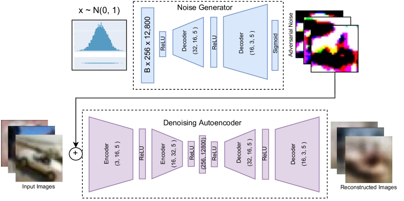
Figure 1: Overview of adversarial noise learning architecture featuring: top-Noise Generator Module $G_{noise}$, bottom- Denoising module $G_{denoise}$.

Our proposed method is outlined in Figure 1. In our approach, we utilise a Denoising Autoencoder Generator ($G_{denoise}$) network together with a GAN-like Noise Generator ($G_{noise}$) network. These are concurrently adversarially trained using the process outlined in Algorithm 1. In a given step, the weights of $G_{noise}$ are updated first with gradient ascent with respect to the reconstruction error so that at any given step, $G_{noise}$ produces differing corruption from the previous step which $G_{denoise}$ then attempts to reverse by optimising the reconstruction error with gradient descent.

Training across dataset $x\in\mathbb{R}^{B\times C\times H\times W}\in X$ where $\{B,C,H,W\}$ represent the batch size, number of channels, height and width, respectively, starts by training the noise generator $G_{noise}$. A linear vector of size $B\times 256$ random variables $\phi$ is sampled from a standard Gaussian normal distribution $\phi\sim N(\mu:0,\sigma:1)$ and fed through $G_{noise}$ to produce noise $n$ of shape $\mathbb{R}^{B\times C\times H\times W}$. The added Sigmoid layer ($\frac{1}{1+e^{-l}}$) on the final layer of $G_{noise}$ binds the noise values continuously between [$0,1$]. We combine the noise $n$ to the input image $x$ using a weighted sum by utilising the linear blending operator $noise(x,n)=\alpha(x)+(1-\alpha)(n)$ where $\alpha$ is randomly sampled on each step within bounds $\alpha\rightarrow[0.2,0.9]\in\mathbb{R}^{+}$. The linear blend operator ensures that the magnitude of the values of $noise(x,n)$ match with the pixel intensities of $x$ and $n$. Values of $x$ are normalised with $0$ mean and unit variance meaning that the values of $noise(x,n)$ are such that $G_{denoise}$ is prevented from discriminating between the noise corrupted pixels and the original image pixels based on differing pixel intensity.

Algorithm 1 Adversarial Noise Training

$\text{W}\{G\}\leftarrow\text{init}$ $\triangleright$ Initialise G randomly

$\text{W}\{N_{G}\}\leftarrow\text{init}$ $\triangleright$ Initialise $N_{G}$ randomly

If alpha is static during training, $G_{noise}$ can theoretically perfectly optimise the generated noise $n$ to destroy all information in image $x\in X$ such that all values in $noise(x,n)$ are set to 1 such that $n=(\frac{1-\alpha\cdot x\in X}{1-\alpha})$. The $noise(x,n)$ cannot converge to all zeros where $n=-(\frac{\alpha\cdot x\in X}{1-\alpha})$ due to the logical argument that the values of noise $n$ produced by $G_{noise}$ are bound to [0,1] $\in\mathbb{R}^{+}$ because of the Sigmoid layer on the output of $G_{noise}$ and $x$ is such that $\forall x_{i}\in x\rightarrow\{0,1\},\exists x_{i}\in x\,|\,x_{i}=1$ implying that if $(x_{i}\in x=1)$ then $n=\frac{-\alpha}{1-\alpha}\Rightarrow n<0\,\,\forall\alpha\therefore n\notin\mathbb{R}^{+}$. To prevent convergence to the trivial solution $n=(\frac{1-\alpha\cdot x\in X}{1-\alpha})$ in our experiments, we: 1) Set the value of $\alpha$ to be randomly continuously sampled for each step during training and 2) The input of $G_{noise}$ is sampled from the Gaussian distribution $N(0,1)$ which applies some level of randomness during sampling.

The $noise(x,n)$ is then used as input to $G_{denoise}$ to reconstruct $x$ from $noise(x,n)$, reversing the corruption caused by $G_{noise}$. The corrupted image $noise_{x,n}$ is encoded to the latent vector $z$ and then subsequently decoded into a synthetic reconstruction $x^{\prime}$.

Adversarial learning is accomplished by the mini-max optimisation between the $G_{denoise}$ and $G_{noise}$ modules. Weights of $G_{denoise}$ are optimised to minimise $\mathcal{L}$, the reconstruction error between $x$ and $x^{\prime}$ whereas the weights of $G_{noise}$ are conversely optimised to maximise $\mathcal{L}$. Loss terms in the overall loss are given scalar regularisation terms $\lambda_{0}$ and $\lambda_{1}$ for losses $\mathcal{L}_{G_{denoise}}$ and $\mathcal{L}_{G_{noise}}$ respectively. The overall optimisation function in this work is:

$$\begin{matrix}argmin&argmax\\ G_{denoise}&G_{noise}\end{matrix}=\mathcal{L}_{G_{denoise}}(x,x^{\prime})\lambda_{0}+\mathcal{L}_{G_{noise}}(x,x^{\prime})\lambda_{1}$$ (1)

This method of training encourages the noise generator to produce masks which optimally corrupt the input. Such optimal noise makes the denoising process more difficult as the denoising module must not only learn meaningful features of the input data, but such learned representations should not carry forward out-of-distribution (anomalous) features to the synthetic reconstruction.

3.1 Loss Function

In our experiments, we find that the use of Focal Frequency Loss (FFL) [Jiang et al., 2021] created higher-fidelity reconstructions and a slight increase in AUC performance. FFL is based on the L2 distance (loss) between the real image $x$ and the generated image $x^{\prime}$ in the Fourier (frequency) domain. Pixel coordinates of $x$ ($x_{i}$) and $x^{\prime}$ ($x^{\prime}_{i}$) are used in conjunction to their respective frequency spectrum coordinates $(x_{i}^{freq}$ & $x^{\prime}$${}_{i}^{freq})$ from the Discrete Fourier Transform (DFT) as follows:

$$F(\vartheta)=(\frac{\vartheta_{i}\cdot\vartheta_{i}^{freq}}{|H|})|\vartheta=\{x,x^{\prime}\}$$ (2)

The loss is defined as the total distance in frequency domain with respect to amplitude and phase in the following formula:

$$\mathcal{L}(x,x^{\prime})=||e^{-i2\pi(F(x))}-e^{-i2\pi(F(x^{\prime}))}||^{2}$$ (3)

Figure 2 shows visually how using an L2 loss loosely approximates the frequency representation of $x$, but fails to capture high-frequency information present in the image. FFL [Jiang et al., 2021] however, can more closely approximate the frequency domain as seen in this figure, the frequency representations of $x$ and $x^{\prime}$ are closely matched. This property makes it highly suitable for use in our reconstruction-driven anomaly detection approach.

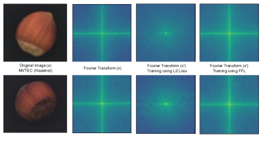
Figure 2: Visualisation of frequency domain after Fourier Transform operation of reconstruction $x^{\prime}$ from input image $x$ both with and without using FFL [Jiang et al., 2021] during training.

4 Experimental Setup

Table 1: Quantitative results (class name indicates AUC, $AUC_{avg}$ of all classes) of models across MNIST [LeCun et al., 2010] (upper) and CIFAR-10 [Krizhevsky and Hinton, 2009] (lower) datasets (Protocol 1).

Model	MNIST
	0	1	2	3	4	5	6	7	8	9	$AUC_{avg}$
VAE [Kingma and Welling, 2014]	0.55	0.10	0.63	0.25	0.35	0.30	0.43	0.18	0.50	0.10	0.34
AnoGAN [Schlegl et al., 2017]	0.61	0.30	0.54	0.44	0.43	0.42	0.48	0.36	0.40	0.34	0.43
EGBAD [Zenati et al., 2018]	0.78	0.29	0.67	0.52	0.45	0.43	0.57	0.40	0.55	0.35	0.50
GANomaly [Akcay et al., 2019b]	0.89	0.65	0.93	0.80	0.82	0.85	0.84	0.69	0.87	0.55	0.79
ADAE [Vu et al., 2019b]	0.95	0.82	0.95	0.89	0.82	0.91	0.89	0.80	0.93	0.63	0.86
DAE	0.84	0.97	0.79	0.64	0.53	0.61	0.66	0.55	0.71	0.57	0.69
DAE+Random Noise	0.84	0.93	0.66	0.66	0.52	0.62	0.72	0.56	0.75	0.53	0.68
DAE+Gaussian Noise $\sim N(0,0.5)$	0.88	0.97	0.77	0.66	0.55	0.62	0.75	0.55	0.71	0.57	0.70
DAE + ALCN	0.97	0.97	0.96	0.89	0.85	0.88	0.92	0.80	0.93	0.76	0.89
Model	CIFAR-10
	Plane	Car	Bird	Cat	Deer	Dog	Frog	Horse	Ship	Truck	$AUC_{avg}$
VAE [Kingma and Welling, 2014]	0.59	0.40	0.52	0.44	0.46	0.50	0.38	0.51	0.64	0.49	0.49
AnoGAN [Schlegl et al., 2017]	0.51	0.49	0.41	0.40	0.34	0.39	0.34	0.41	0.56	0.51	0.44
EGBAD [Zenati et al., 2018]	0.58	0.52	0.39	0.45	0.37	0.49	0.36	0.54	0.42	0.55	0.47
GANomaly [Akcay et al., 2019b]	0.63	0.63	0.51	0.58	0.59	0.62	0.68	0.61	0.62	0.62	0.61
ADAE [Vu et al., 2019a]	0.63	0.73	0.55	0.58	0.50	0.60	0.60	0.61	0.62	0.67	0.61
DAE	0.50	0.68	0.61	0.55	0.69	0.53	0.62	0.60	0.63	0.71	0.61
DAE+Random Noise	0.63	0.53	0.54	0.54	0.65	0.59	0.64	0.55	0.66	0.63	0.60
DAE+Gaussian Noise $\sim N(0,0.5)$	0.57	0.68	0.57	0.54	0.65	0.54	0.55	0.52	0.57	0.53	0.57
DAE + ALCN	0.77	0.71	0.62	0.57	0.72	0.62	0.72	0.60	0.66	0.69	0.67

We present our experimental setup in terms of the benchmark datasets used for evaluation (Section 4.1) and the implementation details of our approach (Section 4.2).

4.1 Datasets

We make use of four established benchmark datasets that are commonplace for evaluation within the anomaly detection domain:

• MNIST [LeCun et al., 2010] : A collection of $69,018$ hand-written single digits from $0$ to $9$ of resolution $28\times 28$. For this dataset we utilise a $80:20$ ($55,209:13,807$) split between training and testing respectively across the data.

• CIFAR-10 [Krizhevsky and Hinton, 2009] : A set of $50,026$ low-resolution ($32\times 32$) images split into ten classes of common objects. A $80:20$ ($40,012:10,012$) split between training and testing sets are utilised across this dataset.

• MVTEC-AD [Bergmann et al., 2019] : Benchmark dataset of $6,809$ images for quality control in industrial visual inspection. The data is composed of fifteen classes of both non-anomalous, defect free objects as well as a set of defective anomalous counter-parts. A $70:30$ split for training and testing respectively is applied for each class.

• Plant Village [Hughes and Salath’e , 2015]: Visual images of the leaves of vital agricultural edible plants together with anomalies containing common visual leaf diseases for each respective plant.

4.2 Implementation Details

Our method is compared across the MNIST [LeCun et al., 2010] and CIFAR-10 [Krizhevsky and Hinton, 2009] datasets due to their inherent simplicity while training as well as giving sufficient bench-marking for the evaluation between the techniques included in this work. Evaluation is conducted in two protocols following from established methods for ‘leave-one-out’ anomaly detection tasks. During protocol 1 (1 vs. rest), one digit is regarded as anomalous and remaining classes are normal as performed by: [Akcay et al., 2018, Akçay et al., 2019, Barker and Breckon, 2021, Zenati et al., 2018, Schlegl et al., 2017, Schlegl et al., 2019]. Protocol 2 (rest vs. 1) as performed by: [Ruff et al., 2018a, Perera et al., 2019, Abati et al., 2019, Salehi et al., 2021, Jewell et al., 2022] is the opposite in that one digit is normal and the nine remaining classes are anomalous.

The split ratio for the data is $80:20$ for training and testing respectively as conducted by [Zenati et al., 2018, Akcay et al., 2019b]. During training, the Adam optimiser is used for both $G_{denoise}$ and $G_{noise}$ with learning rates of $1\times 10^{-5}$ and $8\times 10^{-3}$ respectively. An image resolution of $28\times 28$ is implemented throughout ‘leave-one-out’ anomaly detection tasks [LeCun et al., 2010, Krizhevsky and Hinton, 2009]. We implement a larger resolution of $256\times 256$ across MVTEC [Bergmann et al., 2019] and Plant Village [Hughes and Salath’e , 2015] however. A batch size of 4096 is employed across MNIST and CIFAR-10 and a batch size of 16 is used across MVTEC and plant village during training on an NVidia GTX 1080 TI GPU. We evaluate our method using the Area Under Receiver Operator Characteristic (AUC) metric.

Table 2: Quantitative results ($AUC_{avg}$) of models including ARAE [Salehi et al., 2021] and OLED [Jewell et al., 2022] across MNIST [LeCun et al., 2010] (left) and CIFAR-10 [Krizhevsky and Hinton, 2009] (right) datasets (Protocol 2).

	MNIST	CIFAR-10
Method	AUCavg	AUCavg
DSVDD [Ruff et al., 2018a]	0.948	0.648
OCGAN [Perera et al., 2019]	0.975	0.733
LSA[Abati et al., 2019]	0.975	0.731
ARAE [Salehi et al., 2021]	0.975	0.717
OLED [Jewell et al., 2022]	0.985	0.671
DAE + ALCN	0.989	0.742

5 Results

Table 3: Quantitative results (class name indicates AUC, $AUC_{avg}$ of all classes) of models across MVTEC-AD [Bergmann et al., 2019] dataset.

Model	MVTEC-AD
	Bottle	Cable	Caps.	Carpet	Grid	H’nut	Leath.	M’nut	Pill	Screw	Tile	T’brush	T’sistor	Wood	Zipper	$AUC_{avg}$
VAE [Kingma and Welling, 2014]	0.66	0.63	0.61	0.51	0.52	0.30	0.41	0.66	0.51	1	0.21	0.30	0.65	0.87	0.87	0.58
AnoGAN [Schlegl et al., 2017]	0.80	0.48	0.44	0.34	0.87	0.26	0.45	0.28	0.71	1	0.40	0.44	0.69	0.57	0.72	0.56
EGBAD [Zenati et al., 2018]	0.63	0.68	0.52	0.52	0.54	0.43	0.55	0.47	0.57	0.43	0.79	0.64	0.73	0.91	0.58	0.60
GANomaly [Akcay et al., 2019b]	0.89	0.76	0.73	0.70	0.71	0.79	0.84	0.70	0.74	0.75	0.79	0.65	0.79	0.83	0.75	0.76
Skip-GANomaly [Akçay et al., 2019]	0.93	0.67	0.71	0.79	0.65	0.90	0.90	0.79	0.75	1	0.85	0.68	0.81	0.91	0.66	0.80
DAE+ALCN	0.94	0.84	0.86	0.84	0.97	0.92	0.62	0.86	0.75	1	0.79	0.65	0.73	0.93	0.70	0.83

Extensive comparison of the results of our method compared to prior methods are outlined in Tables 1, 2, 3, 4 and 5. Tables 1 and 2 outline the quantitative results of the DAE+ALCN method across both MNIST [LeCun et al., 2010] and CIFAR-10 [Krizhevsky and Hinton, 2009] ‘leave-one-out tasks’ across both protocol 1 (9 normal/1 anomalous) and protocol 2 (1 normal/9 anomalous). Across the real-world anomaly detection tasks outlined in this paper [Bergmann et al., 2019, Hughes and Salath’e , 2015], Table 3 outlines the quantitative results of our method across the MVTEC-AD [Bergmann et al., 2019] industrial inspection dataset and Table 4 presents the results across the Plant Village dataset [Hughes and Salath’e , 2015].

5.1 Leave One Out Anomaly Detection

5.1.1 Protocol 1

Table 1 outlines the results of each approach across the MNIST and CIFAR-10 datasets. We begin by comparing our vanilla DAE approach without any noise regularisation and this results in an AUC_avg of $0.69$ across MNIST and $0.61$ across CIFAR-10. This is weak compared to other methods in the table. Applying Gaussian noise obtains an AUC_avg of $0.70$ on MNIST and $0.57$ on CIFAR-10. Our DAE+ALCN approach applied to the DAE architecture achieves the best AUC score on 90% of the classes with an average AUC of $0.89$ and produces the best scores on 60% classes of CIFAR-10 with an average AUC score of $0.67$.

5.1.2 Protocol 2

Table 2 presents the results across the protocol 2 variant (1 normal/9 anomalous) across both MNIST and CIFAR-10. Our DAE+ALCN method obtains an AUC_avg of 0.989 across MNIST and an AUC_avg of 0.742 across CIFAR-10, outperforming all prior methods including OLED [Jewell et al., 2022] which uses discrete noise, as previously stated in this work. This gives illumination as to the benefit of using bespoke continuous noise while training.

5.2 Real-world Tasks

Table 4: Quantitative results ($AUC_{avg}$) of models across Plant Village [Hughes and Salath’e , 2015] dataset.

Model	Plant Village
	$AUC_{avg}$
VAE [Kingma and Welling, 2014]	0.65
AnoGAN [Schlegl et al., 2017]	0.65
EGBAD [Zenati et al., 2018]	0.70
GANomaly [Akcay et al., 2019b]	0.73
Skip-GANomaly [Akçay et al., 2019]	0.77
DAE+ALCN	0.77

5.2.1 MVTEC-AD Industrial Inspection Dataset

In this experiment we compare our DAE+ALCN method against prior semi-supervised anomaly detection methods across the MVTEC-AD task [Bergmann et al., 2019] to verify that we can apply our method to a real-world example rather than solely across synthetic and trivial leave-one-out tasks.

The results of this experiment are shown in Table 3. It can be observed that DAE+ALCN obtains the highest average AUC score of $0.83$, outperforming all other methods on $10$ out of the $15$ classes in MVTEC-AD dataset.

Table 5: Comparison of model complexity (number of parameters (millions)) and inference time (milliseconds).

		Model
		DAE	AnoGAN	EGBAD	GANomaly	DAE + ALCN
Parameters (Million)		1.12	233.04	8.65	3.86	9.87
Inference Time/Batch	MNIST	2.36	667	8.02	9.7	4.54
(Millisecond)	CIFAR-10	2.73	611	9.55	10.53	5.23

5.2.2 Plant Village Dataset

The Plant Village dataset [Bergmann et al., 2019] is challenging due to the large intra-class variance present in this dataset. Leaves of a given plant can vary vastly in appearance with respect to shape and colour. As such, it is challenging to map the underlying distribution of the leaves. The quantitative results of methods across this dataset are presented in Table 4. Our DAE+ALCN method obtains an AUC_avg of 0.77 which is the same as that of Skip-GANomaly [Akçay et al., 2019]. Both methods far-outperform prior methods across this dataset.

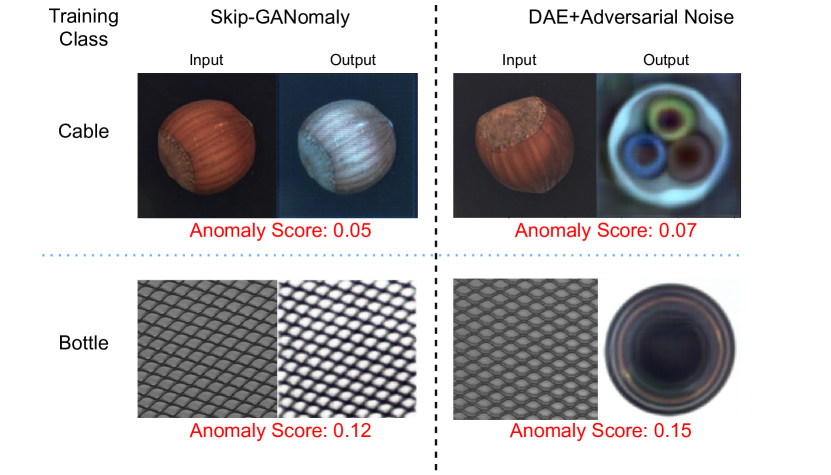
Figure 3: Comparison between Skip-GANomaly[Akcay et al., 2019a] and DAE+Adversarial Noise of feeding vastly out-of-distribution (Hazelnut and Grid) examples through models trained on a different class (Cable and Bottle).

Figure 3 illustrates the results of an input which is an out-of-distribution example through both the Skip-GANomaly [Akçay et al., 2019] and DAE+ALCN into models trained on only another specific class singular (Figure 3, left label). The objective being that Skip-GANomaly [Akçay et al., 2019] and DAE+ALCN should reconstruct out-of-distribution examples within the original class distribution. However, it can be seen in Figure 3 that Skip-GANomaly [Akçay et al., 2019] successfully reconstructs an out-of-distribution example given weight to the conclusion that it has converged to a pass-though identity function and just copies information from input to output (i.e. hazelnut/grid observed in both input + output), despite the fact the model has never been exposed to these class examples in training. For Skip-GANomaly this leads to low anomaly scores of 0.05 and 0.12 for Cable and Bottle respectively. By contrast, our DAE+ALCN architecture, manages to reconstruct such out-of-distribution examples back into the training classes thus resulting in the anomaly scores 0.07 for Cable (0.02 larger than Skip-GANomaly [Akcay et al., 2019a]) and 0.15 for Bottle (0.03 higher than Skip-GANomaly [Akcay et al., 2019a]). This shows that given vastly out-of-distribution examples, the DAE+ALCN network is more robust to misclassification and less prone to a pass-through identity-like reconstruction output.

Overall these experiments show that using our adversarial noise as a regularisation technique can enable even a simple architecture such as the Denoising Autoencoder outlined in Figure 1 to obtain better results than more complex model architectures.

5.3 Model Complexity

An outline of model complexity together with inference time per batch is outlined in Table 5. The DAE+ALCN architecture has $9.87$ Million parameters which is slightly larger than EGBAD [Zenati et al., 2018] which is at $8.65$ Million but still orders of magnitude smaller relative to that of AnoGAN [Schlegl et al., 2017]. The magnitude of our model comes from the noise generation module (ALCN) in addition to the DAE module which is fairly light weight at 1.12 million parameters. This means that during training, the adversarial noising approach outlined in this paper adds a significant memory overhead to the model during training however, has an inference speed of $4$ milliseconds per batch which is significantly faster than the other methods, but generating the noise during inference adds a slight overhead of 2.5ms over the standard DAE architecture.

5.3.1 Qualitative Results

Figure 4 illustrates the qualitative results of DAE+ALCN across different datasets. The first column for each example shows the input images to the model. The second column illustrates the adversarial noise which is added to the input resulting in those images (3rd column). This adversarial noise + input is then fed into DAE and the resulting output after denoising (4th column). Of particular interest are the noise examples across the MNIST [LeCun et al., 2010] and Plant Village [Hughes and Salath’e , 2015] datasets. From Figure 4 we can observe that the adversarial noise tends towards the style/shape of the input data which, when added to the image, adds a large level of input obfuscation (Figure 4 - Input + Noise columns). Despite this, the DAE architecture is able to successfully reconstruct the original input images from this maximally noised version with significant fidelity (Figure 4 - Output columns).

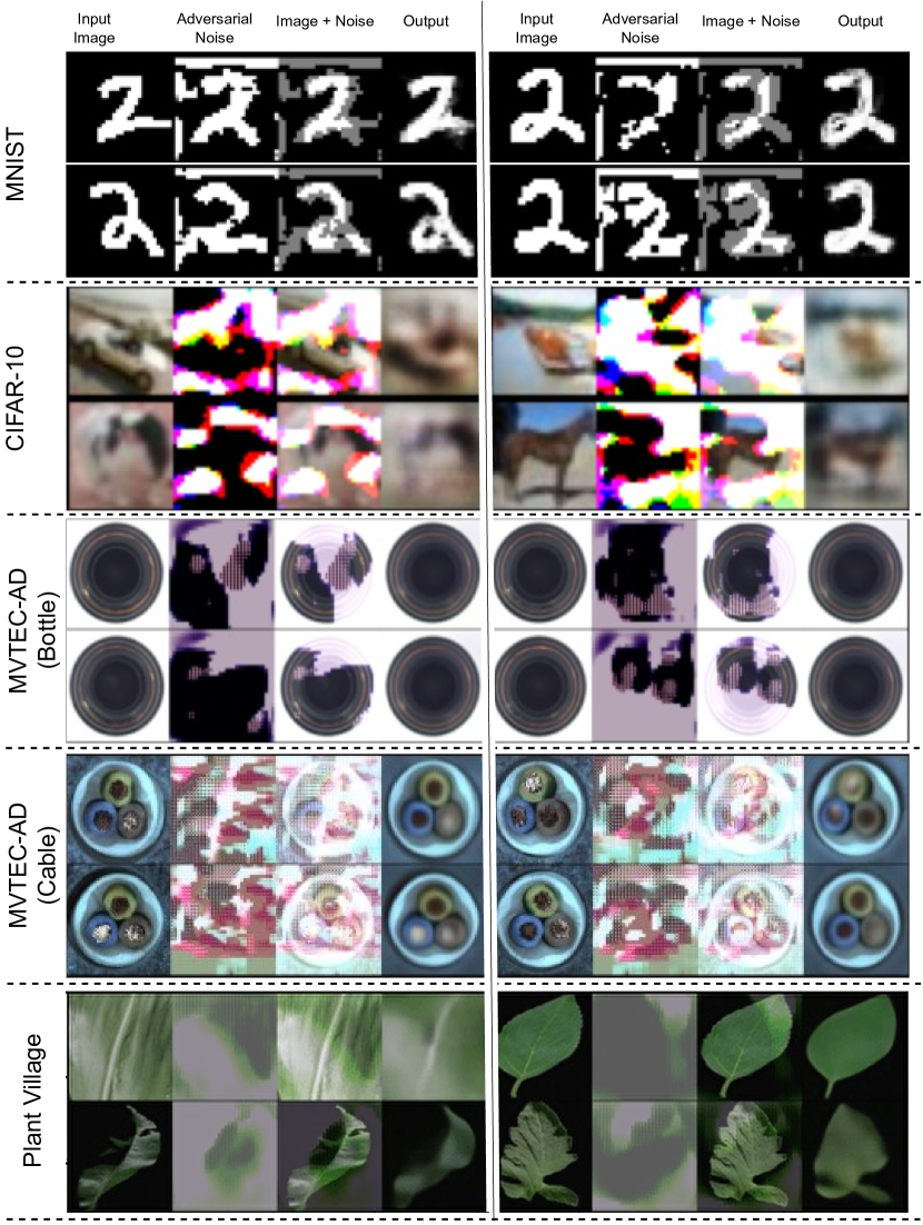
Figure 4: Examples of input image, generated adversarial noise, input + noise addition and resulting reconstructed output (left $\rightarrow$ right).

6 Conclusion

In this work we introduce a novel approach for improved robustness semi-supervised anomaly detection by adversarially training a noise generator to produce maximal continuous noise which is then added to input data. In the same training step, a simple Denoising Autoencoder (DAE) is optimised to reconstruct the denoised, unperturbed input from the noised input. Through this simple approach, we vastly improve performance on semi-supervised anomaly detection tasks across both benchmark ‘leave-one-out’ anomaly and challenging real-world anomaly detection tasks, outperforming prior work in the field. Via ablation, we also show the DAE with adversarial noise approach demonstrates superior performance against prior fixed-parameter noising strategies (random and Gaussian) across the leave-one-out benchmark tasks.

REFERENCES

- Abati et al., 2019 Abati, D., Porrello, A., Calderara, S., and Cucchiara, R. (2019). Latent space autoregression for novelty detection. In Conference on Computer Vision and Pattern Recognition (CVPR), pages 481–490. IEEE Computer Society.
- Adey et al., 2021 Adey, P. A., Akçay, S., Bordewich, M. J., and Breckon, T. P. (2021). Autoencoders without reconstruction for textural anomaly detection. In 2021 International Joint Conference on Neural Networks (IJCNN), pages 1–8. IEEE.
- Akcay et al., 2019a Akcay, S., Atapour-Abarghouei, A., and Breckon, T. (2019a). Skip-ganomaly: Skip connected and adversarially trained encoder-decoder anomaly detection. Proceedings of the International Joint Conference on Neural Networks, July.
- Akcay et al., 2018 Akcay, S., Atapour-Abarghouei, A., and Breckon, T. P. (2018). Ganomaly: Semi-supervised anomaly detection via adversarial training. In Asian conference on computer vision, pages 622–637. Springer.
- Akcay et al., 2019b Akcay, S., Atapour-Abarghouei, A., and Breckon, T. P. (2019b). Ganomaly : semi-supervised anomaly detection via adversarial training. In 14th Asian Conference on Computer Vision, number 11363 in Lecture notes in computer science, pages 622–637. Springer.
- Akçay et al., 2019 Akçay, S., Atapour-Abarghouei, A., and Breckon, T. P. (2019). Skip-ganomaly: Skip connected and adversarially trained encoder-decoder anomaly detection. In 2019 International Joint Conference on Neural Networks (IJCNN), pages 1–8. IEEE.
- Barker and Breckon, 2021 Barker, J. W. and Breckon, T. P. (2021). Panda: Perceptually aware neural detection of anomalies. In International Joint Conference on Neural Networks, IJCNN.
- Bengio et al., 2013 Bengio, Y., Yao, L., Alain, G., and Vincent, P. (2013). Generalized denoising auto-encoders as generative models. arXiv preprint arXiv:1305.6663.
- Bergmann et al., 2019 Bergmann, P., Fauser, M., Sattlegger, D., and Steger, C. (2019). Mvtec ad–a comprehensive real-world dataset for unsupervised anomaly detection. In Proceedings of the IEEE/CVF Conference on Computer Vision and Pattern Recognition, pages 9592–9600.
- Bhowmik et al., 2019 Bhowmik, N., Gaus, Y., Akcay, S., Barker, J. W., and Breckon, T. P. (2019). On the impact of object and sub-component level segmentation strategies for supervised anomaly detection within x-ray security imagery. In 18th IEEE International Conference on Machine Learning and Applications (ICMLA 2019). IEEE.
- Donahue et al., 2019 Donahue, J., Darrell, T., and Philipp, K. (2019). Adversarial feature learning. In 5th International Conference on Learning Representations, ICLR 2017 - Conference Track Proceedings. International Conference on Learning Representations, ICLR.
- Gaus et al., 2019 Gaus, Y. F. A., Bhowmik, N., Akçay, S., Guillén-Garcia, P. M., Barker, J. W., and Breckon, T. P. (2019). Evaluation of a dual convolutional neural network architecture for object-wise anomaly detection in cluttered x-ray security imagery. In 2019 International Joint Conference on Neural Networks (IJCNN), pages 1–8.
- Goodfellow et al., 2014 Goodfellow, I., Pouget-Abadie, J., Mirza, M., Xu, B., Warde-Farley, D., Ozair, S., Courville, A., and Bengio, Y. (2014). Generative adversarial nets. In Ghahramani, Z., Welling, M., Cortes, C., Lawrence, N., and Weinberger, K. Q., editors, Advances in Neural Information Processing Systems, volume 27. Curran Associates, Inc.
- Hughes and Salath’e , 2015 Hughes, D. P. and Salath’e , M. (2015). An open access repository of images on plant health to enable the development of mobile disease diagnostics through machine learning and crowdsourcing. CoRR, abs/1511.08060.
- Jewell et al., 2022 Jewell, J. T., Reza Khazaie, V., and Mohsenzadeh, Y. (2022). One-class learned encoder-decoder network with adversarial context masking for novelty detection. In 2022 IEEE/CVF Winter Conference on Applications of Computer Vision (WACV), pages 2856–2866.
- Jiang et al., 2021 Jiang, L., Dai, B., Wu, W., and Loy, C. C. (2021). Focal frequency loss for image reconstruction and synthesis. In ICCV.
- Kingma and Welling, 2014 Kingma, D. and Welling, M. (2014). Auto-encoding variational bayes. In 2nd International Conference on Learning Representations.
- Krizhevsky and Hinton, 2009 Krizhevsky, A. and Hinton, G. (2009). Learning multiple layers of features from tiny images. Master’s thesis, Department of Computer Science, University of Toronto.
- LeCun et al., 2015 LeCun, Y., Bengio, Y., and Hinton, G. (2015). Deep learning. nature, 521(7553):436–444.
- LeCun et al., 2010 LeCun, Y., Cortes, C., and Burges, C. (2010). Mnist handwritten digit database. ATT Labs [Online]. Available: http://yann.lecun.com/exdb/mnist, 2.
- Pang et al., 2018 Pang, G., Cao, L., Chen, L., and Liu, H. (2018). Learning representations of ultrahigh-dimensional data for random distance-based outlier detection. In Proceedings of the 24th ACM SIGKDD international conference on knowledge discovery & data mining, pages 2041–2050.
- Pang et al., 2019 Pang, G., Shen, C., Jin, H., and Hengel, A. v. d. (2019). Deep weakly-supervised anomaly detection. arXiv preprint arXiv:1910.13601.
- Pathak et al., 2016 Pathak, D., Krahenbuhl, P., Donahue, J., Darrell, T., and Efros, A. A. (2016). Context encoders: Feature learning by inpainting. In Proceedings of the IEEE conference on computer vision and pattern recognition, pages 2536–2544.
- Perera et al., 2019 Perera, P., Nallapati, R., and Xiang, B. (2019). Ocgan: One-class novelty detection using gans with constrained latent representations. In Conference on Computer Vision and Pattern Recognition (CVPR). IEEE Computer Society.
- Ruff et al., 2018a Ruff, L., Vandermeulen, R., Goernitz, N., Deecke, L., Siddiqui, S. A., Binder, A., Müller, E., and Kloft, M. (2018a). Deep one-class classification. In Dy, J. and Krause, A., editors, Proceedings of the 35th International Conference on Machine Learning, volume 80 of Proceedings of Machine Learning Research, pages 4393–4402. PMLR.
- Ruff et al., 2018b Ruff, L., Vandermeulen, R., Goernitz, N., Deecke, L., Siddiqui, S. A., Binder, A., Müller, E., and Kloft, M. (2018b). Deep one-class classification. In International conference on machine learning, pages 4393–4402. PMLR.
- Salehi et al., 2021 Salehi, M., Arya, A., Pajoum, B., Otoofi, M., Shaeiri, A., Rohban, M. H., and Rabiee, H. R. (2021). Arae: Adversarially robust training of autoencoders improves novelty detection. Neural Networks, 144:726–736.
- Schlegl et al., 2019 Schlegl, T., Seeböck, P., Waldstein, S., Langs, G., and Schmidt-Erfurth, U. (2019). f-anogan: Fast unsupervised anomaly detection with generative adversarial networks. Medical Image Analysis, 54:30–44.
- Schlegl et al., 2017 Schlegl, T., Seeböck, P., Waldstein, S. M., Schmidt-Erfurth, U., and Langs, G. (2017). Unsupervised anomaly detection with generative adversarial networks to guide marker discovery. In International conference on information processing in medical imaging, pages 146–157. Springer.
- Thanh-Tung and Tran, 2020 Thanh-Tung, H. and Tran, T. (2020). Catastrophic forgetting and mode collapse in gans. In International Joint Conference on Neural Networks (IJCNN 2020), pages 1–10.
- Vu et al., 2019a Vu, H. S., Ueta, D., Hashimoto, K., Maeno, K., Pranata, S., and Shen, S. (2019a). Anomaly detection with adversarial dual autoencoders.
- Vu et al., 2019b Vu, H. S., Ueta, D., Hashimoto, K., Maeno, K., Pranata, S., and Shen, S. (2019b). Anomaly detection with adversarial dual autoencoders. ArXiv, abs/1902.06924.
- Zenati et al., 2018 Zenati, H., Foo, C., Lecouat, B., Manek, G., and Chandrasekhar, V. (2018). Efficient gan-based anomaly detection. arXiv, abs/1802.06222.
- Zhang et al., 2018 Zhang, Z., Li, M., and Yu, J. (2018). On the convergence and mode collapse of gan. In SIGGRAPH Asia 2018 Technical Briefs, SA ’18, New York, NY, USA. Association for Computing Machinery.
- Zhou and Paffenroth, 2017 Zhou, C. and Paffenroth, R. C. (2017). Anomaly detection with robust deep autoencoders. In Proceedings of the 23rd ACM SIGKDD international conference on knowledge discovery and data mining, pages 665–674.