Jet polarisation in an anisotropic medium

Abstract

We study the evolution of an energetic jet which propagates in an anisotropic quark-gluon plasma, as created in the intermediate stages of ultrarelativistic heavy-ion collisions. We argue that the partons of the jet should acquire a non-zero average polarisation proportional to the medium anisotropy. We first observe that the medium anisotropy introduces a difference between the rates for transverse momentum broadening along the two directions perpendicular to the jet axis. In turn, this difference leads to a polarisation-dependent bias in the BDMPS-Z rates for medium-induced gluon branching. Accordingly, the daughter gluons in a branching process can carry net polarisation even if their parent gluon was unpolarised. Using these splitting rates, we construct kinetic equations which describe the production and transmission of polarisation via multiple branching in an anisotropic medium. The solutions to these equations show that polarisation is efficiently produced via quasi-democratic branchings, but then it is rapidly washed out by the subsequent branchings, due to the inability of soft gluons to keep trace of the polarisation of their parents. Based on that, we conclude that a net polarisation for the jet should survive in the final state if and only if the medium anisotropy is sizeable as the jet escapes the medium.

1 Introduction

The physics of “jet quenching” — a rather general concept which encompasses the ensemble of the modifications suffered by an energetic jet or hadron which propagates through a quark-gluon plasma — represents one of our main sources of information about the properties of the dense QCD medium created in the intermediate stages of ultrarelativistic heavy-ion collisions at RHIC and the LHC Casalderrey-Solana:2007knd ; Qin:2015srf ; Blaizot:2015lma . The theory of jet quenching was originally developed for a limited set of phenomena — collisional transverse momentum broadening and medium-induced radiative energy loss —, for a relatively simple “hard probe” (an energetic parton), and for a weakly-coupled plasma in thermal equilibrium. More recently, the theory and phenomenology of jet quenching have progressively been extended to genuine jets (including vacuum-like and medium-induced parton cascades), to more complex aspects of the jet-medium interactions, like colour decoherence or medium back-reaction, and to a plasma which is far away from thermal equilibrium and might be even strongly coupled. At the same time, the spectrum of associated observables has extended from inclusive quantities like the nuclear suppression of hadron and jet production (largely controlled by the in-medium energy loss), to extremely complex, global, phenomena like the dijet asymmetry (which likely probes all the stages of the in-medium evolution, as well as the fine structure of the medium), and also to fine probes of the jet substructure (which arguably lies within the realm of QCD perturbation theory).

In this paper, we propose another effect that should emerge from the jet interactions in a dense QCD medium: if the medium is anisotropic, then the jet partons should acquire net polarisation. There are several mechanisms for generating such an anisotropy for the quark-gluon plasma created in the intermediate stages of a nucleus-nucleus collision.

The high energy of experiments naturally leads to a rapid longitudinal expansion of the quark-gluon plasma (QGP) medium created in the wake of a collision Bjorken:1982qr . In turn, the expansion of the QGP medium leads to a pronounced anisotropy in the momentum distribution of the medium constituents: their momentum component $p_{z}$ along the collision axis is typically much smaller than the transverse components $p_{x}$ and $p_{y}$ Baier:2000sb . This has interesting consequences for various probes of the medium, such as stronger binding of quarkonia and preferred orientation of the quarks comprising a quarkonium Dumitru:2009ni ; Burnier:2009yu ; Thakur:2012eb ; Dong:2022mbo , angular dependence in energy loss and momentum broadening of heavy quarks Prakash:2021lwt ; Song:2019cqz ; Romatschke:2004au and a modification of the spectrum of dileptons radiated by the plasma Ryblewski:2015hea ; Churchill:2020uvk ; Coquet:2021lca . An anisotropy in the transverse plane is possible as well, especially in not so central collisions where it leads to the elliptic flow of hadrons. This transverse anisotropy will be ignored in our subsequent study.

Another scenario leading to medium anisotropy is inherent in the glasma picture for the early stages Lappi:2006fp . The “glasma” (the precursor of the quark-gluon plasma) is a form of gluonic matter with large occupation numbers, that can be conveniently described in terms of strong, classical, colour fields. The underlying theory (the “colour glass condensate”, or CGC Iancu:2003xm ; Gelis:2010nm ; Gelis:2012ri ; Gelis:2015gza ) predicts that, right after the collision, the distribution of these fields should be strongly anisotropic: their energy density is concentrated within longitudinal (chromo-electric and chromo-magnetic) flux tubes which extend between the recessing nuclei. This anisotropy has been argued to have observable consequences, such as inducing spin polarization of heavy quarks in the glasma Kumar:2022ylt .

In both the case of the QGP medium and of the glasma, the anisotropy is expected to decrease with time. The longitudinal expansion of the QGP medium should compete with elastic collisions among the plasma constituents which redistribute energy and momentum, and thus broaden the originally anisotropic momentum distribution. In the glasma scenario, the longitudinal flux tubes are unstable and should eventually break and transmit their energy to gluons with transverse polarisations. Yet, explicit calculations in both scenarios — lattice calculations for the glasma Berges:2013eia ; Berges:2013fga ; Ipp:2020mjc ; Ipp:2020nfu (that is, classical Yang-Mills theory with initial conditions from the CGC) and, respectively, numerical solutions to kinetic theory for a quark-gluon plasma undergoing boost-invariant longitudinal expansion Kurkela:2015qoa ; Kurkela:2018vqr ; Du:2020dvp and with initial conditions inspired by the “bottom-up” scenario Baier:2000sb — demonstrate that the process of isotropisation proceeds only slowly, so that a sizeable anisotropy persists at all the times that should be relevant for the phenomenology of heavy ion collisions.

Furthermore, both scenarios predict that the medium anisotropy should affect the transverse momentum broadening of an energetic probe (parton or jet) which propagates through the plasma: if the hard probe propagates at central rapidities, say along the $x$ axis, then one should observe an asymmetry between its momentum broadening along the two directions orthogonal to the jet axis, that is, the $y$ and $z$ directions. For the glasma case, lattice calculations of the relevant chromo-electric and chromo-magnetic field correlators (2-point functions of the non-Abelian Lorentz force) have found sizable anisotropy in momentum broadening Ipp:2020mjc ; Ipp:2020nfu . These results are furthermore supported by analytic approximations Carrington:2021dvw ; Carrington:2022bnv .

For a weakly-coupled plasma — the case that we shall focus on in this paper —, the transverse momentum broadening is a consequence of quasi-local elastic collisions and the respective rates — the jet quenching parameters $\widehat{q}_{y}$ and $\widehat{q}_{z}$ — can in principle be computed within perturbation theory. Yet, perturbative calculations for anisotropic plasmas appear to be unstable, due to the non-Abelian analog of the Weibel instabilities (e.g., the polarisation effects introduce a pole at space-like momenta in the retarded propagator) Mrowczynski:1993qm ; Mrowczynski:2016etf ; Hauksson:2020wsm . Whereas for electromagnetic plasma such instabilities are physical and lead to charge filamentation, the fate of instabilities in a non-Abelian plasma is less clear. Classical Yang-Mills simulations on the lattice Berges:2013eia ; Berges:2013fga point to the fact that plasma instabilities do not appear to play a dominant role in the non-equilibrium evolution of the glasma beyond very early times. So, in what follows we shall ignore this problem and assume that the physics of transverse momentum broadening in an anisotropic plasma can be faithfully described in terms of two (generally different) jet quenching parameters, $\widehat{q}_{y}$ and $\widehat{q}_{z}$, even though for the time being we still lack an explicit calculation of these parameters from first principles (see however Arnold:2002zm ; Baier:2008js ; Romatschke:2006bb ; Hauksson:2021okc ).

For simplicity we assume the medium to be homogeneous and static, although it should be possible to incorporate the time-dependence of $\widehat{q}$ due to longitudinal expansion of the medium along the collision axis by following the discussions in Baier:1998yf ; Zakharov:1998wq ; Baier:2000sb ; Arnold:2008iy ; Iancu:2018trm ; Adhya:2019qse ; Caucal:2020uic . Relaxing the assumption of a homogeneous medium introduces new effects in which gradients in temperature and density, as well as net flow of the medium, change the spectrum of radiated partons Barata:2022krd ; Sadofyev:2021ohn ; Andres:2022ndd . These medium inhomogeneities arise naturally in the framework of ideal hydrodynamics where temperature and flow velocity vary in space and time but the medium is everywhere in local thermal equilibrium. Here our goal is to consider genuine non-equilibrium effects and how they modify the spectrum of radiated jet partons. In other words, we consider a QGP medium that is locally out of equilibrium, as e.g. captured by pressure anisotropy and viscous corrections in second order hydrodynamics or non-equilibrium momentum distributions in kinetic theory. Such a non-equilibrium description of the QGP medium is known to be necessary to describe measurements of soft hadrons, see e.g. Romatschke:2007mq . Conveniently, for jet partons at sufficiently high energy where the so-called “harmonic approximation” is valid, the effect of a non-equilibrium medium on the jet is completely captured by the two jet quenching parameters $\widehat{q}_{y}$ and $\widehat{q}_{z}$ such that a detailed microscopic description of the medium is not needed. Our work could be extended to include medium inhomogeneities, in addition to the homogeneous local deviations from equilibrium considered here.

Within this framework, our main observation is that the medium anisotropy should also introduce a polarisation-dependent bias in the rates for medium-induced gluon branching ($g\to gg$). Thus the two daughter gluons can carry non-zero net polarisation even when the parent gluon is unpolarised. We demonstrate this effect within the BDMPS-Z approach, where medium-induced radiation is linked to transverse momentum broadening: parton branching is triggered by multiple soft scattering, leading to a loss of coherence between the daughter partons and their parent. This approach has been originally developed Baier:1996kr ; Baier:1996sk ; Zakharov:1996fv ; Zakharov:1997uu ; Baier:1998kq ; Baier:1998yf ; Zakharov:1998wq ; Wiedemann:1999fq ; Wiedemann:2000za for an isotropic plasma and for the branching of unpolarised partons, but here we shall provide its generalisation to an anisotropic medium and to gluons with definite polarisation states. (We leave the inclusion of quarks to a further study.)

By using the in-medium branching rates for polarised gluons, we construct kinetic equations which describe the evolution of the jet energy and polarisation distributions via multiple branchings. The equation satisfied by the unpolarised distribution is formally the same as for an isotropic medium and its solution is well understood Blaizot:2013hx ; Blaizot:2013vha : it exhibits wave turbulence, that is, the soft gluons rapidly multiply via quasi-democratic branchings, thus allowing for an efficient transfer of energy from the leading parton to low-energy gluons. By using both numerical methods and analytic approximations, we also solve the equation for the polarised distribution which quantifies the degree of polarisation of partons at a given energy. We do this for the case where the leading parton is originally unpolarised. We find that the democratic branchings play an important role for the polarised distribution, with two opposite effects. On one hand, democratic branchings enhance the net polarisation via the branching of unpolarised partons in the presence of the anisotropy. On the other hand, they rapidly randomise the parton polarisation, due to the inability of the soft gluons to keep trace of the polarisation of their parents. The competition between these two tendencies implies that the parton polarisation is created and washed out quasi-locally in energy and time, so that the polarised distribution closely follows the unpolarised one: for sufficiently low energies, these two distributions are simply proportional to each other, with a proportionality coefficient which would vanish for an isotropic medium. In particular, the polarised distribution shows the same characteristic enhancement at low-energies, which is the hallmark of the BDMPS-Z spectrum and also a fixed point of the turbulent parton cascade.

The previous considerations imply that net polarisation of jet partons is only present in the final state if the medium anisotropy survives until the moment when the jet exits the medium. Indeed, at least for the ideal, turbulent cascade that we have studied here, any net polarisation that might be acquired at early stages will be rapidly washed out (via multiple branching) if the medium becomes fully isotropic. Conversely, an experimental observation that indicates a net polarisation of partons in a jet, tells us that the medium anisotropy had persisted until relatively late times. It furthermore gives an indication of the degree of anisotropy as the jet escapes the medium. Measurements of net jet polarisation could be signalled e.g. by a larger-than-expected abundance of non-zero spin hadrons in the jet fragmentation or indirectly through anisotropy in the distribution of hadrons in the jet cone. Thinking further ahead, one could envisage correlating measurements of jet polarisation with jet energy loss, which probes the path length of the jet in medium and thus the time at which a jet escapes the medium. This might give the anisotropy of the medium at different times as the escape time for jets varies between collisions.

So far, we have considered the effect of the medium anisotropy on the polarisation of the partons in a jet, but one could also imagine a scenario where this polarisation is transmitted back to the medium. This is related to the late stage of the bottom-up scenario, which predicts that most of the energy of the medium comes from the quenching of mini-jets in the presence of a highly anisotropic background. The soft gluons created by the decay of the mini-jets are expected to carry net polarisation and thus produce a polarised quark-gluon plasma. It would be interesting to identify observables for such a polarised medium at early stages, like the spin distribution of heavy quarks.

This paper is organised as follows. Sect. 2 presents general considerations about the collisional momentum broadening of an energetic parton propagating through a non-equilibrium, weakly-coupled, quark gluon plasma, which is anisotropic. Our main purpose here is to motivate the relation between the anisotropy in the momentum distributions of the plasma constituents and that in the transverse momentum broadening of the hard probe. Then in Sect. 3 we investigate the consequences of this anisotropy on the branching rates for medium-induced emissions of linearly polarised gluons. After quickly re-deriving the polarised version of the DGLAP splitting functions, we proceed with extending the BDMPS-Z formalism to an anisotropic medium and to polarised gluons. Our main result in that section is a set of polarised in-medium branching rates, shown in Eqs. (54)–(57), whose physical content is briefly discussed in Sect. 3.4. In Sect. 4 we study the evolution of the jet distribution in energy and polarisation via multiple branching. We start by constructing the respective evolution equations — a set of coupled kinetic equations for the polarised and the unpolarised (or total) gluon distributions. The equation for the unpolarised distribution is essentially the same as for an isotropic plasma (it differs only by a rescaling of the time variable), so its solution is well known Blaizot:2013hx . In Sects. 4.2 and 4.3, we also solve the equation for the polarised distribution, via the Green’s function method. Our main results are encoded in Fig. 3 together with the analytic approximation (103), valid for soft gluons. We summarise our conclusions together with some open problems in Sect. 5.

2 Transverse momentum broadening in an anisotropic plasma

For simplicity, we consider a jet made only of gluons. This is a good approximation at large number of colours $N_{c}$. The jet is initiated by a “leading gluon” which propagates along the $x$ axis. The secondary gluons produced via successive gluon branchings are assumed to be quasi-collinear to the leading parton, hence to the $x$ axis. In the BDMPSZ approach, the physics of medium-induced radiation is linked to that of transverse momentum broadening, where by “transverse” we now mean the $(y,z)$ plane, which is perpendicular to the jet direction of motion. Since the jet dynamics is most naturally analysed w.r.t. the jet axis, we shall systematically use this convention from now on: by “transverse” we shall always mean the $(y,z)$ plane, and not the plane $(x,y)$ which is orthogonal to the collision axis. Similarly, the $x$ axis will often be referred to as “longitudinal”.

The “transverse momentum broadening” in this context means that the partons from the jet suffer independent collisions with the plasma constituents, leading to a broadening of their 3-momentum distribution along the $y$ and $z$ directions: the transverse momenta $p_{y}$ and $p_{z}$, as accumulated via collisions, are relatively small ($p_{y}^{2},\,p_{z}^{2}\ll p_{x}^{2}$) and random, with dispersions which grow linearly in time: $\langle p_{y}^{2}\rangle=\widehat{q}_{y}\Delta t$ and $\langle p_{z}^{2}\rangle=\widehat{q}_{z}\Delta t$. The hallmark of an anisotropic plasma is the fact that the rates, $\widehat{q}_{y}$ and $\widehat{q}_{z}$, for transverse momentum broadening along the two transverse directions are not the same:

$$\widehat{q}_{y}\equiv\frac{d\langle p^{2}_{y}\rangle}{dt}\,\neq\,\widehat{q}_{z}\equiv\frac{d\langle p^{2}_{z}\rangle}{dt}\,.$$ (1)

Inspired by recent calculations of momentum broadening in the Glasma Ipp:2020nfu ; Ipp:2020mjc ; Carrington:2021dvw , we shall sometimes assume that $\widehat{q}_{z}>\widehat{q}_{y}$ — the momentum broadening is stronger along the collision axis than perpendicular to it. That said, our subsequent results do not crucially depend upon the sign of the difference $\widehat{q}_{z}-\widehat{q}_{y}$: all that matters is the fact that these quantities are generally different. The limit of an isotropic plasma can be easily obtained from our results by letting $\widehat{q}_{z}=\widehat{q}_{y}\equiv\hat{q}/2$.

Although the physical origin of the anisotropy is not essential for what follows, it is still interesting to understand how the difference between $\widehat{q}_{z}$ and $\widehat{q}_{y}$ may arise in the case of a weakly coupled quark-gluon plasma. To that aim, we shall briefly recall the respective calculation of transverse momentum broadening, with emphasis on the possible sources of anisotropy.

Before that, let us summarise our notations. The Minkowski coordinates of a generic space-time point $x$ will be written as $x^{\mu}=(t,x,y,z)=(t,\vec{x})=(t,x,\bm{x}_{\perp})$, where the 3-vector $\vec{x}\equiv(x,y,z)$ encompasses all the spatial coordinates, while the 2-vector $\bm{x}_{\perp}\equiv(y,z)$ refers to the transverse plane alone. Similarly, for the 4-momentum $p$ we will write $p^{\mu}=(p_{0},p_{x},p_{y},p_{z})=(p_{0},\vec{p})=(p_{0},p_{x},\bm{p}_{\perp})$. To study the interactions between the jet and the medium, it will also be convenient to use light-cone vector notations w.r.t. to the jet ($x$) axis, defined as

$$x^{+}\equiv\frac{t+x}{\sqrt{2}},\quad x^{-}\equiv\frac{t-x}{\sqrt{2}},\quad p^{+}\equiv\frac{p_{0}+p_{x}}{\sqrt{2}},\quad p^{-}\equiv\frac{p_{0}-p_{x}}{\sqrt{2}}\,.$$ (2)

The variable $x^{+}$ plays the role of the LC time, while $p^{+}$ is the LC longitudinal momentum. To simplify wording and notations, we shall generally refer to $x^{+}$ simply as “time” (and use the simpler notation $t\equiv x^{+}$), while $p^{+}$ will be the “energy” (sometimes denoted as $\omega$). Also, we shall ignore the “perp” subscript $\perp$ on transverse vectors whenever there is no possible confusion. In LC notations, the 4-momentum of a parton reads $p^{\mu}=(p^{+},p^{-},\bm{p}_{\perp})$, where $\bm{p}_{\perp}=(p_{y},p_{z})$ is the transverse momentum and $p^{-}=\bm{p}_{\perp}^{2}/2p^{+}$ for an on-shell massless parton.

To study transverse momentum broadening, we consider the propagation of an energetic gluon (the “hard probe”) through a weakly-coupled QGP. The gluon longitudinal momentum $p^{+}$ is assumed to be much larger than both the (longitudinal and transverse) momenta of the plasma constituents and the transverse momentum $\bm{p}_{\perp}$ acquired by the probe via collisions. In this high-energy kinematics, the hard gluon predominantly couples to the light-cone component $A^{-}\equiv(A_{0}-A_{x})/\sqrt{2}$ of the gauge field generated by the plasma constituents. So, for the present purposes, the medium can be described as a random colour field $A^{-}_{a}$ with 2-point correlation function

$$\langle{A}^{-}_{a}(x^{+},x^{-},\bm{x}_{\perp}){A}^{-}_{b}(y^{+},y^{-},\bm{y}_{\perp})\rangle\,=\,\delta_{ab}\delta(x^{+}-y^{+})\,\gamma(\bm{x}_{\perp}-\bm{y}_{\perp}),$$ (3)

where the angular brackets denote the medium average. The restriction to the 2-point function is justified to leading order at weak coupling. The $\delta$–function in colour space, $\delta_{ab}$, follows from gauge invariance, while that in LC time, $\delta(x^{+}-y^{+})$, from Lorentz time dilation (the energetic parton has a poor resolution in $x^{+}$, hence it “sees” the medium correlations as quasi-local in time). The 2-point function is independent of $x^{-}$ and $y^{-}$, since the medium is probed near the trajectory of the energetic parton, at $x^{-}\simeq 0$. This is in agreement with our assumption that the plasma fields $A^{-}_{a}$ carry relatively small longitudinal momenta $k^{+}\ll p^{+}$. In turn, this implies that both the longitudinal momentum $p^{+}$ of the hard gluon and its polarisation are not effected by the medium. Finally, $\gamma(\bm{x}_{\perp}-\bm{y}_{\perp})$ depends only upon the transverse separation $\bm{x}_{\perp}-\bm{y}_{\perp}$ by homogeneity, and is independent of $x^{+}$ because the plasma is assumed to be static. (More general situations, e.g. a plasma which expands along the collisional axis, can be similarly considered.)

In this set-up, the medium anisotropy is encoded in the fact that the 2-point correlation $\gamma(\bm{x}_{\perp}-\bm{y}_{\perp})$ has no rotational symmetry in the transverse plane, that is, it is not just a function of the distance $r\equiv|\bm{x}_{\perp}-\bm{y}_{\perp}|$. When Fourier transformed to transverse momentum space, Eq. (3) becomes (we suppress the irrelevant variables $x^{-}$ and $y^{-}$)

$$\left\langle A^{-}_{a}(x^{+},\bm{k}_{\perp})A^{*-}_{b}(y^{+},\bm{q}_{\perp})\right\rangle=\delta_{ab}\delta(x^{+}-y^{+})(2\pi)^{2}\delta^{(2)}(\bm{k}_{\perp}-\bm{q}_{\perp})\,\tilde{\gamma}(\bm{k}_{\perp})\;.$$ (4)

For an anisotropic case, the function $\tilde{\gamma}(\bm{k}_{\perp})$ (a.k.a. the “collision kernel”) depends upon the orientation of the 2-dimensional vector $\bm{k}_{\perp}=(k_{y},k_{z})$, that is, it separately depends upon its 2 components.

To gain more insight in the structure of $\tilde{\gamma}(\bm{k}_{\perp})$ and thus understand how an anisotropy might be generated, it is instructive to recall the relation between the 2-point function of the field and that of its colour sources (the quarks and gluons from the plasma). Our discussion will be very schematic, since merely intended for illustration purposes. In particular, we shall often ignore the Minkowski and colour indices, and write the gluon correlator simply as $G(x,y)\equiv\langle{A}(x){A}(y)\rangle$. For a plasma which is static and homogeneous, this admits the Fourier representation

$$G(x-y) =\int\frac{{\rm{d}}k^{-}}{2\pi}\,{\rm e}^{-ik^{-}(x^{+}-y^{+})}\int\frac{{\rm{d}}k^{+}}{2\pi}\,{\rm e}^{-ik^{+}(x^{-}-y^{-})}\int\frac{{\rm{d}}^{2}\bm{k}_{\perp}}{(2\pi)^{2}}\,{\rm e}^{i\bm{k}_{\perp}\cdot(\bm{x}_{\perp}-\bm{y}_{\perp})}\,G(k^{+},k^{-},\bm{k}_{\perp})$$

$$\simeq\int\frac{{\rm{d}}k^{-}}{2\pi}\,{\rm e}^{-ik^{-}(x^{+}-y^{+})}\int\frac{{\rm{d}}k^{+}}{2\pi}\int\frac{{\rm{d}}^{2}\bm{k}_{\perp}}{(2\pi)^{2}}\,{\rm e}^{i\bm{k}_{\perp}\cdot(\bm{x}_{\perp}-\bm{y}_{\perp})}\,G(k^{+},k^{-}=0,\bm{k}_{\perp}),$$ (5)

where the second lines was obtained by using $x^{-}\simeq y^{-}\simeq 0$ (more precisely, $x^{-}\sim y^{-}\sim 1/p^{+}$ with $p^{+}\gg k^{+}$) and by approximating $k^{-}\simeq 0$ inside the correlator: this is appropriate since the LC times $x^{+}$ and $y^{+}$ take relatively large values $x^{+}\sim y^{+}\sim 1/p^{-}$, with $p^{-}=\bm{p}_{\perp}^{2}/2p^{+}$ much smaller than the typical values of $k^{-}$. Hence, the integral is controlled by unusually small values of $k^{-}$ (to avoid large oscillations of the phase ${\rm e}^{-ik^{-}(x^{+}-y^{+})}$, so the function $G$ inside the integrand can be evaluated at $k^{-}=0$. This condition $k^{-}=0$, or $k_{0}=k_{x}$, shows that we consider space-like modes of the gluon correlator: $k^{2}=k_{0}^{2}-\vec{k}^{2}=-k_{\perp}^{2}<0$, where $\vec{k}=(k_{x},k_{y},k_{z})=(k_{x},\bm{k}_{\perp})$.

The integral over $k^{-}$ generates the $\delta$–function $\delta(x^{+}-y^{+})$, so the final result in Eq. (2) is indeed consistent with Eq. (4), with the following representation for the collision kernel:

$$\tilde{\gamma}(\bm{k}_{\perp})\simeq\int\frac{{\rm{d}}k^{+}}{2\pi}\,G^{--}(k^{+},k^{-}=0,\bm{k}_{\perp}).$$ (6)

For space-like modes, the statistical 2-point function of the gluon field emitted by the plasma constituents has the general structure

$$G(k)\,=\,|G_{R}(k)|^{2}\,\Pi(k),$$ (7)

where $G_{R}(k)$ is the retarded propagator and $\Pi(k)$ is the gluon polarisation tensor. This structure can be understood as follows: introducing the colour charge density $\rho(k)$ of the plasma constituents, the (event-by-event) gauge field is schematically obtained as $A(k)=G_{R}(k)\rho(k)$, hence its 2-point function has indeed the structure (7) with $\Pi(k)=\langle\rho(k)\rho(-k)\rangle$ (the charge-charge correlator). The retarded propagator too is modified by polarisation effects, via the retarded version of the polarisation tensor: $G_{R}^{-1}=G_{0,R}^{-1}+\Pi_{R}$, with $G_{0,R}$ the free retarded propagator.

Due to the mobility of the colour charges, the polarisation tensor is non-local, i.e $\Pi(k)$ is a non-trivial function of the 4-momentum $k^{\mu}=(k_{0},\vec{k})$. This non-locality reflects the momentum distribution of the plasma constituents: when this distribution happens to be anisotropic, it implies a corresponding anisotropy in the “collision kernel” $\tilde{\gamma}(\bm{k}_{\perp})$. To be more specific, let us remind the reader of the expression of the polarisation tensor in the Hard Thermal Loop (HTL) approximation.

The HTLs describe the response of the medium constituents to long-wavelength excitations, such as the soft gluons exchanged in elastic collisions (see Refs. Blaizot:2001nr ; Kapusta:2006pm for pedagogical discussions). Originally introduced in the context of thermal equilibrium Braaten:1989mz ; Frenkel:1989br ; Blaizot:1993zk , the HTLs have subsequently been extended to more general, non-equilibrium, situations, that can be still described in terms of quasi-particles and their occupation numbers. (See notably Refs. Arnold:2002zm ; Mrowczynski:2000ed ; Romatschke:2003ms ; Mrowczynski:2004kv ; Hauksson:2021okc for HTL studies in the context of anisotropic plasmas.) For a static and homogeneous plasma, we shall denote these occupation numbers as $f_{g}(\vec{p})$ and $f_{q}(\vec{p})$ for (on-shell) gluons and quarks, respectively. In thermal equilibrium, the quasi-particles have typical energies and momenta of the order of the temperature, $p_{0}=p\sim T$ (with $p=|\vec{p}|$), whereas the typical momenta exchanged via (small-angle) elastic collisions are much softer: $k_{0},k\sim gT\ll T$. Out of equilibrium, we shall assume that a similar hierarchy exists, between the “hard” momenta of the medium constituents and the “soft” exchanges. Under these assumptions, the leading-order expression of the polarisation tensor for soft gluons is given by the gluon HTL, which reads (after restoring the Minkowski indices)

$$\Pi^{\mu\nu}(k)\,=4\pi g^{2}\int\frac{{\rm{d}}^{3}\vec{p}}{(2\pi)^{3}}\left[N_{c}f_{g}(\vec{p})(1+f_{g}(\vec{p}))+N_{f}f_{q}(\vec{p})(1-f_{q}(\vec{p}))\right]v^{\mu}v^{\nu}\,\delta(v\cdot k),$$ (8)

where $v^{\mu}\equiv p^{\mu}/p=(1,\vec{v})$ with $\vec{v}=\vec{p}/p$ (the particle velocity). The piece proportional to $N_{c}$ ($N_{f}$) is the gluon (quark) contribution. The support of the $\delta$–function reflects the microscopic origin of the plasma polarisation — the absorption of the soft gluon by a plasma constituent (“Landau damping”): for this process to be kinematically allowed, the soft gluon must be space-like. The argument of the $\delta$–function can be rewritten as $v\cdot k=(p\cdot k)/p$ with

$$p\cdot k=p^{+}k^{-}+p^{-}k^{+}-\bm{p}_{\perp}\cdot\bm{k}_{\perp}\simeq p^{-}k^{+}-\bm{p}_{\perp}\cdot\bm{k}_{\perp},$$ (9)

where the last, approximate, equality, uses $k^{-}=0$, as in Eq. (2). So long as the transverse momentum $\bm{p}_{\perp}$ of the hard parton is kept fixed, the integrand of Eq. (8) is clearly anisotropic in the transverse plane: it depends upon the azimuthal angle $\phi$ between $\bm{k}_{\perp}$ and $\bm{p}_{\perp}$.

In thermal equilibrium, this anisotropy is washed out by the integral over $\bm{p}_{\perp}$, because the thermal distributions — the Bose-Einstein distribution $f_{g}^{\rm eq}(p)$ for gluons and the Fermi-Dirac distribution $f_{q}^{\rm eq}(p)$ for quarks — are themselves isotropic. It is then straightforward to perform the integral over $p$ and find

$$\Pi^{\mu\nu}(k_{0},\vec{k}) \,=2\pi m_{D}^{2}T\int\frac{{\rm{d}}\Omega}{4\pi}\,v^{\mu}v^{\nu}\delta(k_{0}-\vec{v}\cdot\vec{k}),$$ (10)

where the angular integral runs over the directions of the unit vector $\vec{v}$ and

$$m_{D}^{2}=\,(2N_{c}+N_{f})\frac{g^{2}T^{2}}{6}\,,$$ (11)

is the Debye mass. We also used the following integrals for the thermal distributions:

$$\int{\rm{d}}p\,p^{2}f_{q}(p)(1-f_{q}(p))=-T\int{\rm{d}}p\,p^{2}\frac{{\rm{d}}f_{q}}{{\rm{d}}p}=2T\int{\rm{d}}p\,pf_{q}(p)=\frac{\pi^{2}T^{3}}{6}\,,$$

$$\int{\rm{d}}p\,p^{2}f_{g}(p)(1+f_{g}(p))=-T\int{\rm{d}}p\,p^{2}\frac{{\rm{d}}f_{g}}{{\rm{d}}p}=2T\int{\rm{d}}p\,pf_{g}(p)=\frac{\pi^{2}T^{3}}{3}\,.$$ (12)

Still in thermal equilibrium, the statistical self-energy $\Pi$ and the retarded one $\Pi_{R}$ are related via the KMS condition, which implies (for soft gluon modes with $k_{0}\ll T$)

$$\Pi^{\mu\nu}(k)\,=\,-\frac{T}{k_{0}}\,2\,{\rm Im}\,\Pi_{R}^{\mu\nu}(k)\,.$$ (13)

Using this relation together with Eq. (10) one finds the expected result for the imaginary part of the retarded HTL Blaizot:2001nr ; Kapusta:2006pm . The Debye mass $m_{D}^{2}$ acts as a screening mass in the propagator of the longitudinal gluon and also in the collision kernel.

Specifically, in thermal equilibrium and to leading-order in perturbative QCD, the collision kernel (6) has been computed as Aurenche:2002pd ; CaronHuot:2008ni

$$\tilde{\gamma}(k_{\perp})\,=\,\frac{1}{\sqrt{2}}\,\frac{Tm_{D}^{2}}{k_{\perp}^{2}(k_{\perp}^{2}+m_{D}^{2})},$$ (14)

where the first (second) terms inside the parentheses refers to the exchange of a transverse (longitudinal) gluon. For relatively large momenta $k_{\perp}\gg m_{D}$, we recognise the characteristic power tail $\sim 1/k_{\perp}^{4}$ of Rutherford scattering, but the singularity at low momenta $k_{\perp}\to 0$ gets milder ($1/k_{\perp}^{2}$ instead of $1/k_{\perp}^{4}$), due to Debye screening for $k_{\perp}\lesssim m_{D}$.

Out of equilibrium, the momentum distributions can be anisotropic for a variety of reasons. One natural mechanism in that respect is the expansion of the plasma along the collision ($z$) axis: the partons liberated in a heavy-ion collision should follow straight-line trajectories and segregate themselves in $z$ according to their longitudinal velocity $v_{z}=p_{z}/p$. This “free-streaming” scenario, expected to hold at very early stages, leads to an anisotropic momentum distribution, which is strongly oblate: $\langle p_{z}^{2}\rangle\ll\langle p^{2}\rangle$ in the local rest frame. With increasing time, the interactions are expected to become more important (notably, due to the emission of soft gluons) and to reduce the anisotropy via elastic collisions. In this “bottom-up” scenario for thermalisation Baier:2000sb , that is supported by numerical solutions to kinetic theory Kurkela:2015qoa ; Kurkela:2018vqr ; Du:2020dvp , the plasma is predicted to slowly evolve towards isotropisation and eventually reach thermal equilibrium at very large times — much larger than the lifetime of the quark-gluon plasma produced in heavy ion collisions.

During this slow approach to isotropisation at late stages, it seems legitimate to neglect the time-dependence of the anisotropy. In what follows, we shall make the stronger assumption that the medium is static as a whole — that is, we also neglect its longitudinal expansion along the collision axis. This assumption is only intended for simplicity and can be relaxed in further work: the effects of the medium expansion can be included in an adiabatic approximation (e.g. by allowing the jet quenching parameters, $\widehat{q}_{y}$ and $\widehat{q}_{z}$, to be time-dependent), as in previous studies Baier:1998yf ; Zakharov:1998wq ; Baier:2000sb ; Arnold:2008iy ; Salgado:2002cd ; Salgado:2003gb ; Adhya:2019qse ; Iancu:2018trm ; Caucal:2020uic which assumed an isotropic medium. For such a static but anisotropic medium, the momentum distributions of the plasma constituents take the generic form

$$f_{\nu}(\vec{p})\,=\,F\left(\sqrt{p^{2}+\nu p_{z}^{2}}\right),$$ (15)

where the parameter $\nu$ characterises the strength of the anisotropy: a positive value $\nu>0$ implies an oblate distribution with $\langle p_{z}^{2}\rangle<\langle p^{2}_{x}\rangle=\langle p^{2}_{y}\rangle$. The precise form of the function $F$ is unimportant for what follows (in some calculations, this is taken to be the equilibrium distribution Romatschke:2003ms ; Hauksson:2021okc ). Using a momentum distribution such as Eq. (15) in the general expressions in Eqs. (6), (7), (10), one would then expect to obtain an anisotropic collision kernel for momentum broadening $\widetilde{\gamma}(\mathbf{k}_{\perp})$ from first principles. In practice this is hindered by e.g. plasma instabilities which are beyond the scope of this paper, see e.g. Hauksson:2021okc for further discussion.

We now return to our energetic gluon probe and examine the effects of the collisions on its transverse momentum distribution. This problem has been studied at length in the literature and here we shall only focus on the new aspects which emerge when the medium is anisotropic. We would like to compute compute the probability density ${\cal P}(\Delta\bm{p}_{\perp},\Delta t)$ for the gluon to acquire a transverse momentum $\Delta\bm{p}_{\perp}$ after crossing the medium along a distance (or LC time) $\Delta t$. The calculation is most conveniently formulated in the transverse coordinate representation, which allows for an efficient treatment of multiple scattering: the in-medium propagation of the test particle is governed by a 2-dimensional Schrödinger equation describing quantum diffusion in the random field $A^{-}$ (see Appendix A). As well known, this Schrödinger equation admits a formal solution in terms of a path integral. By multiplying two such solutions — for the gluon in the direct amplitude (DA) and in the complex-conjugate amplitude (CCA), respectively – and averaging over the random field $A^{-}$ according to Eq. (4), one effectively builds the $S$-matrix $S(\bm{r},\Delta t)$ for the elastic scattering of a gluon-gluon dipole with transverse size $\bm{r}$. The probability density of interest is finally obtained as the following Fourier transform (see Appendix A for details)

$${\cal P}(\Delta\bm{p}_{\perp},\Delta t)=\int{\rm{d}}^{2}\bm{r}\,{\rm e}^{-i\Delta\bm{p}_{\perp}\cdot\bm{r}}\,S(\bm{r},\Delta t)\,,\qquad S(\bm{r},\Delta t)\,\equiv\,{\rm e}^{-g^{2}{N_{c}}\Delta t[\gamma(0)-\gamma(\bm{r})]}.$$ (16)

The dipole $S$–matrix obeys $S(r\to 0)\to 1$ (“colour transparency”), which ensures the proper normalisation for the probability density:

$$\int\frac{{\rm{d}}^{2}\bm{p}_{\perp}}{(2\pi)^{2}}\,{\cal P}(\bm{p}_{\perp},\Delta t)=1.$$ (17)

We are interested in the multiple-scattering regime where the distance $\Delta t$ travelled by the probe through the medium is much larger than the mean free path $\lambda_{\rm mfp}$ between two successive collisions. Accordingly, the momentum $\Delta p_{\perp}\equiv|\Delta\bm{p}_{\perp}|$ accumulated during $\Delta t$ is typically much larger than the Debye mass $m_{D}$ (the typical momentum transfer in a single collision): $\Delta p_{\perp}\gg m_{D}$. In this regime, the function in the exponent of $S$, that is,

$$\gamma(0)-\gamma(\bm{r})=\int\frac{{\rm{d}}^{2}\bm{k}_{\perp}}{(2\pi)^{2}}\left(1-{\rm e}^{i\bm{k}_{\perp}\cdot\bm{r}}\right)\tilde{\gamma}(\bm{k}_{\perp}),$$ (18)

has a logarithmic domain of integration at $m_{D}\ll k_{\perp}\ll 1/r\sim\Delta p_{\perp}$. Indeed, the polarisation effects (in or out of thermal equilibrium) cannot modify the fact that $\tilde{\gamma}(\bm{k}_{\perp})\propto 1/k_{\perp}^{4}$ for sufficiently large momenta $k_{\perp}\gg m_{D}$. Hence, in the leading-logarithmic approximation which only keeps the contribution enhanced by the large logarithm $\ln\frac{1}{rm_{D}}$, one can evaluate the integral by expanding the exponential ${\rm e}^{i\bm{k}_{\perp}\cdot\bm{r}}$ within the integrand. It is natural to assume reflexion symmetry, e.g. $\tilde{\gamma}(-k_{y},k_{z})=\tilde{\gamma}(k_{y},k_{z})$ — that is, $\tilde{\gamma}(\bm{k}_{\perp})$ is truly a function of $|k_{y}|$ and $|k_{z}|$. Then the linear terms and also the crossed quadratic terms in the expansion cancel after the integration and the leading logarithmic contribution comes from the diagonal quadratic terms:

$$\gamma(0)-\gamma(\bm{r})\simeq\frac{1}{2}\int\frac{{\rm{d}}^{2}\bm{k}_{\perp}}{(2\pi)^{2}}\left(k_{y}^{2}r_{y}^{2}+k_{z}^{2}r_{z}^{2}\right)\tilde{\gamma}(\bm{k}_{\perp}).$$ (19)

This finally implies

$$S(\bm{r},\Delta t)\simeq\exp\left\{-\frac{\Delta t}{2}\left(\widehat{q}_{y}r_{y}^{2}+\widehat{q}_{z}r_{z}^{2}\right)\right\},$$ (20)

where

$$\widehat{q}_{y}\equiv\frac{g^{2}N_{c}}{2}\int\frac{{\rm{d}}^{2}\bm{k}_{\perp}}{(2\pi)^{2}}\,k_{y}^{2}\,\tilde{\gamma}(\bm{k}_{\perp}),$$ (21)

together with a similar expression for $\widehat{q}_{z}$. As already mentioned, the above integral has a logarithmic divergence at large values of $k_{\perp}$ which must be cut off at $k_{\perp}\sim 1/r$. For instance, for a plasma in thermal equilibrium, we can use (14) to deduce $\widehat{q}_{y}=\widehat{q}_{z}=\hat{q}/2$, with

$$\hat{q}\simeq\frac{\alpha_{s}N_{c}Tm_{D}^{2}}{\sqrt{2}}\int^{1/r^{2}}\frac{{\rm{d}}k_{\perp}^{2}}{k_{\perp}^{2}+m_{D}^{2}}\simeq\sqrt{2}\alpha_{s}N_{c}Tm_{D}^{2}\ln\frac{1}{rm_{D}}\,.$$ (22)

Similar logarithmic dependences upon the dipole size $r$ are expected for both $\widehat{q}_{y}$ and $\widehat{q}_{z}$ in the case of an anisotropic plasma. Such dependences complicate the final Fourier transform to transverse momentum space, cf. Eq. (16). A common approximation at this level, known as the “harmonic approximation”, consists in ignoring this residual $r$-dependence Baier:1998yf ; Zakharov:1998wq . This is appropriate for describing the effects of multiple soft scattering. With this approximation, the Fourier transform is easily computed as

$${\cal P}(\Delta\bm{p}_{\perp},\Delta t)=\frac{2\pi}{\sqrt{\widehat{q}_{y}\widehat{q}_{z}}\Delta t}\,\exp\left\{-\frac{(\Delta p_{y})^{2}}{2\widehat{q}_{y}\Delta t}-\frac{(\Delta p_{z})^{2}}{2\widehat{q}_{z}\Delta t}\right\}.$$ (23)

This Gaussian probability distribution immediately implies the expected results for anisotropic momentum broadening, namely $\langle\Delta p_{y}^{2}\rangle=\widehat{q}_{y}\Delta t$ and $\langle\Delta p_{z}^{2}\rangle=\widehat{q}_{z}\Delta t$.

Incidentally, the above discussion shows that Eq. (20) can be rewritten as

$$S(\Delta t,\bm{r})\simeq\exp\left\{-\frac{1}{2}\left(r_{y}^{2}\langle\Delta p_{y}^{2}\rangle+r_{z}^{2}\langle\Delta p_{z}^{2}\rangle\right)\right\}.$$ (24)

This formula is more general than our present considerations at weak coupling: it is also found when non-perturbatively evaluating the Wilson loop which reduces to our gluon-gluon dipole correlator in the LC gauge $A^{+}=0$ (see e.g. Eq. (31) in Ipp:2020mjc ). This formula was used in Ipp:2020mjc to extract $\langle\Delta p_{y}^{2}\rangle$ and $\langle\Delta p_{z}^{2}\rangle$ from real-time lattice simulations of the Glasma. In our perturbative approach, this formula comes together with results like Eq. (21), which relate $\widehat{q}_{y}$ and $\widehat{q}_{z}$ to the microscopic structure of the medium.

3 Polarised gluon splitting in an anisotropic plasma

Besides providing transverse momentum broadening, the transverse “kicks” received by a test parton via collisions in the plasma also have the effect to trigger radiation. The medium-induced radiation in the kinematical range of interest is controlled by the BDMPS-Z mechanism Baier:1996kr ; Baier:1996sk ; Zakharov:1996fv ; Zakharov:1997uu ; Baier:1998kq ; Baier:1998yf ; Zakharov:1998wq ; Wiedemann:1999fq ; Wiedemann:2000za , which takes into account the coherence effects associated with multiple soft scattering during the quantum formation of an emission. This mechanism is effective so long as the characteristic formation time $t_{f}=\sqrt{2\omega/\hat{q}}$, with $\omega$ the energy of the emitted gluon and $\hat{q}$ the jet quenching parameter, is much larger than the parton mean free path $\lambda_{\rm mfp}=m_{D}^{2}/\hat{q}$ between two successive collisions, but smaller than the medium size $L$ available to the parent parton. (Note that we ignore the medium anisotropy for these physical considerations: its effects, to be later discussed, do not modify the general picture.) These conditions imply an energy window $\omega_{\rm BH}\ll\omega\lesssim\omega_{c}$. The lower limit $\omega_{\rm BH}\equiv m_{D}^{4}/2\hat{q}$, corresponding to $t_{f}\simeq\lambda_{\rm mfp}$, separates from the Bethe-Heitler regime, where emissions are triggered by a single, soft, scattering. The upper limit $\omega_{c}\equiv\hat{q}L^{2}/2$ is the maximal energy of a gluon emitted via multiple soft scattering, for which $t_{f}\simeq L$.

In what follows, we shall focus on the typical gluon emissions, those with energies much smaller than $\omega_{c}$, but much larger than $\omega_{\rm BH}$. Such emissions have relatively short formation times, $t_{f}(\omega)\ll L$, hence a large emission probability,

$$\omega\frac{{\rm{d}}\mathcal{P}}{{\rm{d}}\omega}\,\simeq\,\frac{\alpha_{s}C_{R}}{\pi}\,\frac{L}{t_{f}(\omega)}\,=\,\frac{\alpha_{s}C_{R}}{\pi}\,\sqrt{\frac{\omega_{c}}{\omega}}\,,$$ (25)

so for them the effects of multiple branchings are expected to be important Blaizot:2012fh ; Blaizot:2013hx ; Blaizot:2013vha . On the other hand, such emissions occur quasi-instantaneously, hence multiple emissions can be simply resummed by solving appropriate rate equations Blaizot:2013hx ; Blaizot:2013vha . The only non-trivial ingredient of these equations is the emission rate (the emission probability per unit time), which in turn can be inferred from the BDMPS-Z spectrum for a single gluon emission with $\omega\ll\omega_{c}$. So, our main objective in this section is to generalise the BDMPS-Z branching rate to the case of an anisotropic plasma and to gluons with fixed polarisations. As we shall see, this generalisation brings no conceptual difficulties: the treatment of multiple soft scattering in an anisotropic medium has already been discussed in the previous section and the polarisation dependence of the branching rate is fully encoded in the (leading-order) DGLAP splitting functions, which are well known — including for polarised partons (see e.g. Ellis:1996mzs and Sect. 3.1 below).

After this preparation, let us start our study of polarised medium-induced gluon branching ($g\to gg$) in an anisotropic plasma. Consider the branching process $a\to b+c$, where the gluon labels $a,b$ and $c$ encompass all the relevant “quantum numbers” (longitudinal and transverse momenta, polarisation, and colour). Both the parent gluon and the two daughter ones are assumed to be on-shell, yet the branching is kinematically allowed due to the collisions in the medium. As already argued, the parton longitudinal momenta (“energies”) are not significantly changed by the interactions with the medium, so we can assume energy conservation: $p^{+}_{a}=p^{+}_{b}+p^{+}_{c}$. It is then convenient to use the simpler notation $\omega\equiv p^{+}_{a}$ and introduce the splitting fractions $\zeta\equiv p^{+}_{b}/\omega$ and $1-\zeta=p^{+}_{c}/\omega$ of the daughter gluons. The transverse momentum balance is more subtle: this is conserved at the QCD splitting vertex, which is local in time, but not also for the overall branching process, which is non-local. Physically, this non-conservation is associated with the collisional broadening during the formation time, estimated as $\Delta k_{\perp}^{2}\simeq\hat{q}t_{f}$ with $t_{f}=\sqrt{2\zeta(1-\zeta)\omega/\hat{q}}$. Mathematically, this is expressed by the fact that the QCD splitting vertices occur at different times, $t_{1}$ and $t_{2}$, in the DA and, respectively, the CCA, so they generally involve different transverse momenta on their external legs: this difference accounts for the additional momentum broadening during the interval $t_{2}-t_{1}$.

Before we discuss the full process including medium effects, let us consider the QCD splitting vertex for gluons with linear polarisations (this will be an ingredient of the complete calculation).

3.1 DGLAP splitting functions for linearly polarised gluons

As announced, the special geometry of the medium, which distinguishes between momentum broadening along the $y$ and the $z$ directions, makes it useful to work with linearly polarised states which are aligned along these 2 directions. To specify these states, we first need to fix the gauge. The natural gauge for describing quantum evolution in LC time $x^{+}$ is the LC gauge $A^{+}=0$ (with $A^{+}\equiv(A_{0}+A_{x})/\sqrt{2}$ of course). In this gauge and in LC notations, $\epsilon^{\mu}=(\epsilon^{+},\epsilon^{-},\bm{\epsilon}_{\perp})$, the polarisation vectors describing linear polarisations along the two transverse directions $y$ and $z$ read as follows (for a gluon with transverse momentum $\bm{k}_{\perp}$ and longitudinal momentum $k^{+}$):

$$\epsilon^{\mu}(k,\lambda)=\left(0,\,\frac{\bm{\epsilon}_{\lambda}\cdot\bm{k}_{\perp}}{k^{+}}\,,\,\bm{\epsilon}_{\lambda}\right),\quad\bm{\epsilon}_{y}=(1,0),\ \ \bm{\epsilon}_{z}=(0,1)\,,$$ (26)

where $\lambda$ is the polarisation index: $\lambda=y$ or $z$. These vectors obey $k\cdot\epsilon(k,\lambda)=0$.

The QCD vertex for the $g\to gg$ branching process has the familiar structure

$$V_{abc}^{\mu\nu\rho}(p_{a},p_{b},p_{c})=igf^{abc}\left[g^{\mu\nu}(p_{a}+p_{b})^{\rho}+g^{\nu\rho}(-p_{b}+p_{c})^{\mu}+g^{\rho\mu}(-p_{c}-p_{a})^{\nu}\right],$$ (27)

where we use the convention that the momentum $p_{a}$ flows towards the vertex, while $p_{b}$ and $p_{c}$ flow away from the vertex; hence, momentum conservation reads $p_{a}=p_{b}+p_{c}$. Notice that, with a slight abuse of notations, the indices $a,b$ and $c$ are used both as labels for the 3 gluons, and as the respective colour indices in the adjoint representation. When computing the branching amplitude, this vertex is projected onto the polarisation vectors for the three external gluons, that is, $\epsilon^{\mu}_{a}\equiv\epsilon^{\mu}(p_{a},\lambda_{a})$ for the parent gluon and similarly for the two daughter gluons. After using momentum conservation ($p_{a}=p_{b}+p_{c}$) and the fact that $\epsilon_{a}\cdot p_{a}=\epsilon_{b}\cdot p_{b}=\epsilon_{c}\cdot p_{c}=0$, the result of this projection can be written as Ellis:1996mzs

$$\epsilon_{a}^{\mu}\epsilon_{b}^{\nu}\epsilon_{c}^{\rho}\,V^{abc}_{\mu\nu\rho}(p_{a},p_{b},p_{c})=igf^{abc}\Gamma_{a\rightarrow bc}\,,$$ (28)

with the new vertex $\Gamma_{a\rightarrow bc}$ defined as

$$\Gamma_{a\rightarrow bc}\equiv 2\left[\left(\epsilon_{a}\cdot\epsilon_{b}\right)\left(\epsilon_{c}\cdot p_{b}\right)-\left(\epsilon_{b}\cdot\epsilon_{c}\right)\left(\epsilon_{a}\cdot p_{b}\right)-\left(\epsilon_{c}\cdot\epsilon_{a}\right)\left(\epsilon_{b}\cdot p_{c}\right)\right].$$ (29)

Notice that the “minus” components (e.g. $p_{a}^{-}$) of the parton 4-momenta do not contribute to this vertex, due to our use of the LC gauge.

From Eq. (26), one easily finds

$$\epsilon_{a}\cdot\epsilon_{b}=-\bm{\epsilon}_{\lambda_{a}}\cdot\bm{\epsilon}_{\lambda_{b}}=-\delta_{\lambda_{a}\lambda_{b}}\,,$$ (30)

(and similarly for the other pairs of gluons); this is simply the statement that two different polarisation states (e.g., $\lambda_{a}=y$ and $\lambda_{b}=z$) are orthogonal to each other.

To compute dot products like $\epsilon_{a}\cdot p_{b}$, it is useful to introduce the relative transverse momentum between the 2 daughter partons (or between one daughter parton and its parent), defined as

$$\bm{P}\,\equiv\,(1-\zeta)\bm{p}_{b}-\zeta\bm{p}_{c}\,=\,\bm{p}_{b}-\zeta\bm{p}_{a}\,=\,(1-\zeta)\bm{p}_{a}-\bm{p}_{c}\,,$$ (31)

where the second and third equalities follow from transverse momentum conservation ($\bm{p}_{a}=\bm{p}_{b}+\bm{p}_{c}$). One then easily finds

$$\epsilon_{a}\cdot p_{b} \,=\zeta\bm{p}_{a}\cdot\bm{\epsilon}_{\lambda_{a}}-\bm{p}_{b}\cdot\bm{\epsilon}_{\lambda_{a}}=-\bm{P}\cdot\bm{\epsilon}_{\lambda_{a}}\,,$$

$$\epsilon_{c}\cdot p_{b} \,=\frac{\zeta}{1-\zeta}\,\bm{p}_{c}\cdot\bm{\epsilon}_{\lambda_{c}}-\bm{p}_{b}\cdot\bm{\epsilon}_{\lambda_{c}}=-\frac{\bm{P}\cdot\bm{\epsilon}_{\lambda_{c}}}{1-\zeta}\,,$$

$$\epsilon_{b}\cdot p_{c} \,=\frac{1-\zeta}{\zeta}\,\bm{p}_{b}\cdot\bm{\epsilon}_{\lambda_{b}}-\bm{p}_{c}\cdot\bm{\epsilon}_{\lambda_{b}}=\frac{\bm{P}\cdot\bm{\epsilon}_{\lambda_{b}}}{\zeta}\,.$$ (32)

The final result of these manipulations can be compactly written us

$$\Gamma_{a\rightarrow bc}(\bm{P},\zeta)=2\left[\delta_{\lambda_{a}\lambda_{b}}\,\frac{P_{c}}{1-\zeta}-\delta_{\lambda_{b}\lambda_{c}}P_{a}+\delta_{\lambda_{a}\lambda_{c}}\,\frac{P_{b}}{\zeta}\right].$$ (33)

As manifest from this result, the QCD vertex projected onto the gluon polarisation states depends upon the gluon transverse momenta only via the relative transverse momentum $\bm{P}=(P_{y},P_{z})$.

The (medium-induced) branching probability to be presented in the next subsection will involve the product of the vertex (33) in the DA times a similar vertex, but evaluated at a different value, $\overline{\bm{P}}$, of the relative momentum, in the CCA. The polarisation states for the external gluon are identical for the 2 vertices, since polarisations cannot change via soft scattering with the medium constituents. Since the polarisation indices can only take two values, $\lambda_{a,b,c}=y$ or $z$, one can distinguish between 8 possible polarised splitting functions, conveniently grouped in 4 cases (unless otherwise stated, in the equations below, there is no summation over repeated indices):

(i) when all 3 gluons have the same polarisation, $\lambda_{a}=\lambda_{b}=\lambda_{c}$, one finds

$$\Gamma_{a\rightarrow aa}(\bm{P},\zeta)\Gamma_{a\rightarrow aa}(\bar{\bm{P}},\zeta)=\frac{4P_{a}\bar{P}_{a}}{\zeta(1-\zeta)}\left[\frac{1-\zeta}{\zeta}+\frac{\zeta}{1-\zeta}+\zeta(1-\zeta)\right];$$ (34)

(ii) when $\lambda_{a}=\lambda_{b}\neq\lambda_{c}$ (e.g. $\lambda_{a}=\lambda_{b}=y$, whereas $\lambda_{c}=z$), one finds

$$\Gamma_{a\rightarrow ac}(\bm{P},\zeta)\Gamma_{a\rightarrow ac}(\bar{\bm{P}},\zeta)=\frac{4P_{c}\bar{P}_{c}}{(1-\zeta)^{2}}\,;$$ (35)

(iii) when $\lambda_{a}=\lambda_{c}\neq\lambda_{b}$:

$$\Gamma_{a\rightarrow ba}(\bm{P},\zeta)\Gamma_{a\rightarrow ba}(\bar{\bm{P}},\zeta)=\frac{4P_{b}\bar{P}_{b}}{\zeta^{2}}\,;$$ (36)

(iv) when $\lambda_{a}\neq\lambda_{b}=\lambda_{c}$:

$$\Gamma_{a\rightarrow bb}(\bm{P},\zeta)\Gamma_{a\rightarrow bb}(\bar{\bm{P}},\zeta)=4P_{a}\bar{P}_{a}.$$ (37)

As a final check, let us show that, when summing over polarisation states for all gluons, we recover the familiar expression of the DGLAP splitting function for unpolarised gluons:

$$\frac{1}{2}\sum_{\lambda_{a,b,c}=y,z}\Gamma_{a\rightarrow bc}(\bm{P},\zeta)\Gamma_{a\rightarrow bc}(\bar{\bm{P}},\zeta)=\frac{4\bm{P}\cdot\bar{\bm{P}}}{\zeta(1-\zeta)}\left[\frac{1-\zeta}{\zeta}+\frac{\zeta}{1-\zeta}+\zeta(1-\zeta)\right]$$ (38)

where $\bm{P}\cdot\bar{\bm{P}}=P_{y}\bar{P}_{y}+P_{z}\bar{P}_{z}$. This is indeed the expected result in the unpolarised case Ellis:1996mzs ; Blaizot:2012fh .

3.2 BDMPS-Z branching rate in an anisotropic medium

We shall now construct the medium-induced branching rate for polarised gluons propagating through an anisotropic plasma by generalising the corresponding results for unpolarised gluons which split in an isotropic medium. To that aim, we shall use the path-integral formulation of the BDMPS-Z approach (see e.g. the presentations in Casalderrey-Solana:2011ule ; Blaizot:2012fh ). More precisely, we follow the analysis in Ref. Blaizot:2012fh , which includes a detailed discussion of the transverse momentum dependence of the branching rate. This is indeed important for our purposes, since the polarisation effects depend upon the flow of transverse momentum at the splitting vertices, as previously explained.

The medium-induced branching rate for polarised gluons has the same general structure as in the unpolarised case, except for the fact that it includes the polarised splitting vertices introduced in the previous subsection. Specifically (see Eq. (5.1) in Ref. Blaizot:2012fh )

$$\frac{d\mathcal{P}_{a\rightarrow bc}}{d\zeta dt} \,=\frac{g^{2}N_{c}}{8\pi\omega^{2}\zeta(1-\zeta)}\,\mathrm{Re}\,\int_{0}^{L}d\Delta t\int\frac{d^{2}\bm{P}}{(2\pi)^{2}}\int\frac{d^{2}\bar{\bm{P}}}{(2\pi)^{2}}$$

$$\qquad\times\Gamma_{a\rightarrow bc}(\bm{P},\zeta)\,\Gamma_{a\rightarrow bc}(\bar{\bm{P}},\zeta)\,\tilde{S}^{(3)}(\Delta t,\bm{P},\bar{\bm{P}}),$$ (39)

where we recall that $\omega\equiv p_{a}^{+}$ is the LC longitudinal momentum of the parent parton, $\zeta\equiv p_{b}^{+}/\omega$ is the splitting fraction of gluon $b$, $1-\zeta$ is the corresponding fraction for gluon $c$, and the “time” variables like $t$ or $\Delta t$ are truly light-cone times, cf. Eq. (2). The integration variable $\Delta t\equiv t_{2}-t_{1}$ is the difference between the splitting times (the temporal locations of the QCD vertices) in the direct amplitude (DA) and the complex conjugate amplitude (CCA), respectively. In writing Eq. (3.2), we implicitly assumed that both $t_{1}$ and $t_{2}$ lie inside the medium, that is, we ignored the possibility that the parent gluon splits already before entering the medium, or after exiting from it. This is indeed legitimate for the typical emissions, which have relatively low energies $\zeta(1-\zeta)\omega\ll\omega_{c}$ and therefore short formation times $t_{f}\ll L$. In the present context, the formation time $t_{f}$ is the typical value of $\Delta t$, as fixed by the integrations in Eq. (3.2).

The branching rate in Eq. (3.2) keeps trace of the energies and the polarisation states of the participating gluons, but not of their transverse momenta which are integrated over. More precisely, the integrations run over the relative transverse momenta at the splitting vertices, that is, $\bm{P}$ in the DA (cf. Eq. (31)) and $\bar{\bm{P}}$ in the CCA. As already explained, the difference between $\bm{P}$ and $\bar{\bm{P}}$ reflects the momentum transferred by the medium during the formation time $\Delta t$.

The medium effects are encoded in the 3-point function $\tilde{S}^{(3)}(\Delta t,\bm{P},\bar{\bm{P}})$ which describes the dynamics of the branching system during the time interval $\Delta t$. This is a three point function since it refers to the three gluons which “co-exist” during $\Delta t$: the two daughter gluons in the DA (where the splitting occured at $t_{1}$) and the parent gluon in the CCA (which splits only later, at $t_{2}=t_{1}+\Delta t$). This 3-point function controls the values for $\Delta t$, $P_{\perp}$ and $\bar{P}_{\perp}$. It is most conveniently computed via a Fourier transform from the transverse coordinate representation, that is,

$$\tilde{S}^{(3)}(\Delta t,\bm{P},\bar{\bm{P}})=\int d^{2}\bm{u}\int d^{2}\bm{v}\,e^{i\bm{u}\cdot\bm{P}}e^{-i\bm{v}\cdot\bar{\bm{P}}}\,{S}^{(3)}(\Delta t,\bm{u},\bm{v}).$$ (40)

Indeed, as discussed in the previous section and also in Appendix A, the transverse coordinate representation is better suited for a study of the propagation of a test particle which undergoes multiple scattering off the plasma constituents. Each of the three gluons included in $S^{(3)}$ undergoes 2-dimensional quantum diffusion in the presence of the (Gaussian) random potential $A^{-}$. The formal solution to this quantum diffusion problem can be given a path integral representation, shown in Appendix A. The function ${S}^{(3)}(\Delta t,\bm{u},\bm{v})$ is built by multiplying 3 such solutions (for the 3 gluons involved in the branching process) and then averaging over the random potential according to Eq. (4). The ensuing path integral can be explicitly computed in a “harmonic approximation” which consists in ignoring the logarithmic dependence of the jet quenching parameters $\widehat{q}_{y}$ and $\widehat{q}_{z}$ upon the transverse separations between the 3 partons (recall the discussion after Eq. (22)).

The path integral representation for ${S}^{(3)}(\Delta t,\bm{u},\bm{v})$ is well known for the case of an isotropic plasma. In the harmonic approximation, it reads (see e.g. Eq. (B.26) in Ref. Blaizot:2012fh )

$$S^{(3)}(\Delta t,\bm{u},\bm{v})=\int_{\bm{r}(t=0)=\bm{u}}^{\bm{r}(t=\Delta t)=\bm{v}}\mathcal{D}\bm{r}\exp\left\{iM\int_{0}^{\Delta t}dt\;\left[\frac{\dot{\bm{r}}^{2}}{2}+\frac{\Omega^{2}\bm{r}^{2}}{2}\right]\right\},$$ (41)

where $\bm{r}(t)=\big{(}r_{y}(t),r_{z}(t)\big{)}$ is a 2-dimensional path in the $(y,z)$ plane and we denoted

$$M\equiv\zeta(1-\zeta)\omega,\qquad\Omega^{2}\equiv i\,[1-\zeta(1-\zeta)]\frac{\hat{q}}{2M}\,.$$ (42)

As suggested by these notations, the path integral (41) is formally the same as the solution to the Schrödinger equation for a non-relativistic particle with mass $M$ propagating in a harmonic potential with complex frequency $\Omega$. As generally for a harmonic oscillator, the motions along different directions (here, $y$ and $z$) are independent from each other. This makes the generalisation of (41) to an anisotropic plasma quite straightforward: it suffices to replace

$$\hat{q}\bm{r}^{2}=\hat{q}(r_{y}^{2}+r_{z}^{2})\ \to\ \frac{\widehat{q}_{y}}{2}\,r_{y}^{2}+\frac{\widehat{q}_{z}}{2}\,r_{z}^{2}\,$$ (43)

where the factors $1/2$ are related to our normalisation conventions in Eq. (1) (namely, the isotropic limit is obtained as $\widehat{q}_{z}=\widehat{q}_{y}=\hat{q}/2$). Then the original 2-dimensional path integral factorises into two independent 1-dimensional such integrals, which are easily evaluated (since Gaussian), to yield

$$\begin{split}S^{(3)}(\Delta t,\bm{u},\bm{v})&=\sqrt{\frac{(1-i)\widehat{k}_{y}^{2}}{4\pi\sinh\Omega_{y}\Delta t}}\exp\left[\frac{(i-1)\widehat{k}_{y}^{2}}{4\sinh\Omega_{y}\Delta t}\left((u_{y}^{2}+v_{y}^{2})\cosh\Omega_{y}\Delta t-2u_{y}v_{y}\right)\right]\\ &\times\sqrt{\frac{(1-i)\widehat{k}_{z}^{2}}{4\pi\sinh\Omega_{z}\Delta t}}\exp\left[\frac{(i-1)\widehat{k}_{z}^{2}}{4\sinh\Omega_{z}\Delta t}\left((u_{z}^{2}+v_{z}^{2})\cosh\Omega_{z}\Delta t-2u_{z}v_{z}\right)\right]\end{split}$$ (44)

where

$$\begin{split}\Omega_{y}\equiv\frac{1+i}{\sqrt{2}}\sqrt{\frac{\widehat{q}_{y}[1-\zeta(1-\zeta)]}{\zeta(1-\zeta)\omega}}\end{split}$$ (45)

and

$$\widehat{k}_{y}^{2}\equiv\sqrt{2\zeta(1-\zeta)\omega\,\widehat{q}_{y}[1-\zeta(1-\zeta)]},$$ (46)

and similarly for $\Omega_{z}$ and $\widehat{k}_{z}^{2}$. As expected, Eq. (44) reduces to the well-known result in the literature in the isotropic limit (see Eq. (B.27) in Ref. Blaizot:2012fh ).

As anticipated, the correlation function (44) determines the natural values of the time difference $\Delta t$: when $\Delta t$ is large enough for either $|\Omega_{y}|\Delta t>1$, or $|\Omega_{z}|\Delta t>1$, this correlator decreases exponentially, since e.g. $1/(\sinh\Omega_{y}\Delta t)\propto\exp\{-\Delta t/t_{f,y}\}$ for large $\Delta t$; here,

$$t_{f,y}\,\equiv\,\frac{1}{\mathrm{Re}\,\Omega_{y}}\,=\,\sqrt{\frac{2\zeta(1-\zeta)\omega}{\widehat{q}_{y}[1-\zeta(1-\zeta)]}}\,,$$ (47)

together with a similar expression for $t_{f,z}$. In the isotropic case, $t_{f,y}=t_{f,z}\equiv t_{f}$ is naturally interpreted as the formation time for medium-induced gluon branching. For an anisotropic medium, the corresponding role is played by the smallest among $t_{f,y}$ and $t_{f,z}$ (which corresponds to the largest among $\widehat{q}_{y}$ and $\widehat{q}_{z}$). That is, the formation time is controlled by the direction along which the transverse momentum broadening is strongest. After also performing the Fourier transforms in Eq. (40), one can infer the typical values for the (anisotropic) transverse momentum broadening during formation: one thus finds $\langle P_{y}^{2}\rangle=\langle\bar{P}_{y}^{2}\rangle=\widehat{q}_{y}[1-\zeta(1-\zeta)]t_{f}$, with $t_{f}={\rm min}(t_{f,y},\,t_{f,z})$, and similarly for the $z$ components.

3.3 Medium-induced splitting rates for polarised gluons

Even though the Fourier transform in Eq. (40) would be straightforward to compute (in the harmonic approximation), this is actually not needed for computing the branching rate (3.2). Indeed, given the structure of the QCD vertices in Eqs. (34)–(37), it is enough to compute

$$\,\int\frac{d^{2}\bm{P}}{(2\pi)^{2}}\int\frac{d^{2}\bar{\bm{P}}}{(2\pi)^{2}}\,P_{y}\bar{P}_{y}\,\tilde{S}^{(3)}(\Delta t,\bm{P},\bar{\bm{P}})=\partial_{u_{y}}\partial_{v_{y}}S^{(3)}(\Delta t,\bm{u},\bm{v})\Big{|}_{\bm{u}=\bm{v}=0}$$ (48)

$$\quad=2\pi\left[\frac{(1-i)\widehat{k}_{y}^{2}}{4\pi\sinh\Omega_{y}\Delta t}\right]^{3/2}\left[\frac{(1-i)\widehat{k}_{z}^{2}}{4\pi\sinh\Omega_{z}\Delta t}\right]^{1/2}\ \ \mathop{\longrightarrow}\limits_{\Delta t\to 0}\ \ 2\pi\left[\frac{1}{2\pi}\frac{1-i}{1+i}\,\frac{\zeta(1-\zeta)\omega}{\Delta t}\right]^{2}\,,$$

together with a similar double integral with $P_{y}\bar{P}_{y}\to P_{z}\bar{P}_{z}$.

In the second line of Eq. (49), we have also shown the behaviour of the result in the limit $\Delta t\to 0$, to emphasise the fact that the subsequent integration over $\Delta t$ (cf. Eq. (3.2)) would generate a linear divergence $\int d\Delta t/(\Delta t)^{2}$ from the inferior limit of the integral at $\Delta t=0$. To understand the origin of this divergence and also the way to cure it, let us observe that this limit $\Delta t\to 0$ is in fact equivalent to the vacuum limit $\widehat{q}_{a}\to 0$ (with $a=y$ or $z$): indeed, $\Delta t$ enters the previous results only via the products $\Omega_{y}\Delta t$ and $\Omega_{z}\Delta t$, and $\Omega_{a}\propto\sqrt{\widehat{q}_{a}}$. Hence, the divergence observed when $\Delta t\to 0$ is related to the fact that our results also include vacuum-like radiation (bremsstrahlung) and, moreover, they do that in a wrong way: gluon emissions in the vacuum can occur at all times $-\infty<t_{1},\,t_{2}<\infty$, and when all the regions in $t_{1}$ and $t_{2}$ are included, the overall result must vanish (since energy-momentum conservation forbids an on-shell parton to decay into two other on-shell partons). Hence, the fact that our results seem to admit a non-trivial (and even divergent) “vacuum-limit” is unphysical — this is due to the fact that we restricted the time integrations to $0<t_{1},\,t_{2}<L$, which is indeed appropriate for the (relatively soft) medium-induced emissions, but not also for the vacuum-like emissions. The way to cure this is however obvious: we are anyway interested in medium-induced emissions alone, so it is enough the subtract the “vacuum-limit” from our results.

As an example, let us exhibit the calculation of the decay rate for the process $y\to z,z$ — that is, a parent gluon with linear polarisation along the $y$ axis decays into 2 gluons polarised along the $z$ axis. Using the respective splitting function from Eq. (37) together with Eqs. (3.2) and (49), and the subtraction of the vacuum contribution as above discussed, we are left with

$$\frac{d\mathcal{P}_{y\rightarrow zz}}{d\zeta dt} =\frac{g^{2}N_{c}}{2\pi\omega^{2}\zeta(1-\zeta)}\,\mathrm{Re}\int_{0}^{L}d\Delta t\int\frac{d^{2}\bm{P}}{(2\pi)^{2}}\int\frac{d^{2}\bar{\bm{P}}}{(2\pi)^{2}}\,P_{y}\bar{P}_{y}\,\tilde{S}^{(3)}(\Delta t,\bm{P},\bar{\bm{P}})$$ (49)

$$=\frac{g^{2}N_{c}}{\omega^{2}\zeta(1-\zeta)}\,\mathrm{Re}\int_{0}^{L}d\Delta t\left\{\left[\frac{(1-i)\widehat{k}_{y}^{2}}{4\pi\sinh\Omega_{y}\Delta t}\right]^{3/2}\left[\frac{(1-i)\widehat{k}_{z}^{2}}{4\pi\sinh\Omega_{z}\Delta t}\right]^{1/2}-\left[\frac{1}{2\pi}\frac{1-i}{1+i}\,\frac{M}{\Delta t}\right]^{2}\right\},$$

where we recall that $M=\zeta(1-\zeta)\omega$. The remaining integral over $\Delta t$ is now well defined. Since the integrand is exponentially suppressed when $\Delta t\gg t_{f}$ with $t_{f}\ll L$ (recall our assumption that $M\ll\omega_{c}$), one can extend the upper limit to infinity without loss of accuracy. Then the above integral is conveniently rewritten as

$$\mathrm{Re}\int_{0}^{\infty}d\Delta t\left\{\cdots\right\}=\,\frac{[\zeta(1-\zeta)\omega]^{3/2}}{2(2\pi)^{2}}\,\sqrt{2[1-\zeta(1-\zeta)]}\,\big{(}\widehat{q}_{y}\widehat{q}_{z}\big{)}^{1/4}f\left(\sqrt{\widehat{q}_{z}/\widehat{q}_{y}}\right),$$ (50)

where we defined

$$f(a)\equiv\int_{0}^{\infty}dx\;\left[\frac{1}{a^{1/2}x^{2}}-\frac{1}{\sinh^{1/2}ax\,\sinh^{3/2}x}\right].$$ (51)

The isotropic limit $\widehat{q}_{z}=\widehat{q}_{y}=\hat{q}/2$ corresponds to $a=1$ and then one finds $f(1)=1$. For a medium which is only weakly anisotropic, $\Delta\widehat{q}\ll\hat{q}$, with $\Delta\widehat{q}\equiv\widehat{q}_{z}-\widehat{q}_{y}$ and $\hat{q}\equiv\widehat{q}_{z}+\widehat{q}_{y}$, $a\simeq 1+\Delta\widehat{q}/\hat{q}$ is close to one, and

$$f(a)\simeq 1-\frac{a-1}{4}\,\simeq\,1-\frac{\Delta\widehat{q}}{4\hat{q}}=1-\frac{1}{4}\,\frac{\widehat{q}_{z}-\widehat{q}_{y}}{\widehat{q}_{z}+\widehat{q}_{y}}\qquad\mbox{when}\qquad\Delta\widehat{q}\ll\hat{q}\,.$$ (52)

In the second part of this paper, we shall study the energy distribution of polarised partons, as produced via multiple medium-induced branchings. To that aim, we will need the inclusive rate for the transition $a\to b$ between 2 given polarisation states $a$ and $b$. We shall compute this inclusive rate starting with the exclusive rate for the process $a\to b,c$ and summing over the two possible polarisation states for the gluon $c$. That is, the daughter gluon that we will explicitly follow is that with splitting fraction $\zeta$. (So long as the energy of the measured daughter gluon is specified as well, the two daughter gluons cannot be confused with each other.) We are thus led to define

$$\frac{d\mathcal{P}_{a\rightarrow b}}{d\zeta dt}\,\equiv\,\sum_{\lambda_{c}=y,z}\frac{d\mathcal{P}_{a\rightarrow bc}}{d\zeta dt}\,,$$ (53)

where it is understood that the parent gluon has energy $\omega$ and polarisation state $\lambda_{a}$, whereas the measured daughter gluon has energy $\zeta\omega$ and polarisation state $\lambda_{b}$.

It is straightforward although a bit tedious to derive the analog of Eqs. (49)–(50) for all the relevant $a\to b$ transition channels. The results are suggestively written as follows

$$\begin{split}\frac{d\mathcal{P}_{z\rightarrow z}}{d\zeta dt}={\bar{\alpha}_{s}}\frac{(\widehat{q}_{y}\widehat{q}_{z})^{1/4}}{\sqrt{2\omega}}A(\widehat{q}_{z}/\widehat{q}_{y})\,\gamma(\zeta)\left[\mathcal{F}^{0}_{z\rightarrow z}(\zeta)+G(\widehat{q}_{z}/\widehat{q}_{y})\mathcal{F}^{1}_{z\rightarrow z}(\zeta)\right].\end{split}$$ (54)

$$\begin{split}\frac{d\mathcal{P}_{z\rightarrow y}}{d\zeta dt}={\bar{\alpha}_{s}}\frac{(\widehat{q}_{y}\widehat{q}_{z})^{1/4}}{\sqrt{2\omega}}A(\widehat{q}_{z}/\widehat{q}_{y})\,\gamma(\zeta)\left[\mathcal{F}^{0}_{z\rightarrow y}(\zeta)-G(\widehat{q}_{z}/\widehat{q}_{y})\,\mathcal{F}^{1}_{z\rightarrow y}(\zeta)\right]\end{split}$$ (55)

$$\begin{split}\frac{d\mathcal{P}_{y\rightarrow z}}{d\zeta dt}={\bar{\alpha}_{s}}\frac{(\widehat{q}_{y}\widehat{q}_{z})^{1/4}}{\sqrt{2\omega}}A(\widehat{q}_{z}/\widehat{q}_{y})\,\gamma(\zeta)\left[\mathcal{F}^{0}_{y\rightarrow z}(\zeta)+G(\widehat{q}_{z}/\widehat{q}_{y})\,\mathcal{F}^{1}_{y\rightarrow z}(\zeta)\right]\end{split}$$ (56)

$$\begin{split}\frac{d\mathcal{P}_{y\rightarrow y}}{d\zeta dt}={\bar{\alpha}_{s}}\frac{(\widehat{q}_{y}\widehat{q}_{z})^{1/4}}{\sqrt{2\omega}}A(\widehat{q}_{z}/\widehat{q}_{y})\,\gamma(\zeta)\left[\mathcal{F}^{0}_{y\rightarrow y}(\zeta)-G(\widehat{q}_{z}/\widehat{q}_{y})\,\mathcal{F}^{1}_{y\rightarrow y}(\zeta)\right]\end{split}$$ (57)

where $\bar{\alpha}_{s}\equiv\alpha_{s}N_{c}/\pi$, $\gamma(\zeta)$ is a splitting kernel which summarises the $\zeta$–dependence of the medium-induced radiation,

$$\gamma(\zeta)=\frac{\left[1-\zeta(1-\zeta)\right]^{1/2}}{\zeta^{1/2}(1-\zeta)^{1/2}},$$ (58)

and the new functions $A(\widehat{q}_{z}/\widehat{q}_{y})$ and $G(\widehat{q}_{z}/\widehat{q}_{y})$ are defined as

$$A(\widehat{q}_{z}/\widehat{q}_{y})\equiv\frac{1}{2}\left[f(a)+f(1/a)\right]\,,\qquad G(\widehat{q}_{z}/\widehat{q}_{y})\equiv\frac{f(1/a)-f(a)}{f(a)+f(1/a)}\,,$$ (59)

with $a=\sqrt{\widehat{q}_{z}/\widehat{q}_{y}}$ and the function $f(a)$ introduced in Eq. (51). In the isotropic limit ($a\to 1$), one has $A\to 1$ and $G\to 0$. For an anisotropic medium, $G(a)$ is positive when $a>1$ and negative when $a<1$. In particular, in the limit of a small anisotropy, $\Delta\widehat{q}\ll\hat{q}$, one finds $G(\widehat{q}_{z}/\widehat{q}_{y})\simeq\Delta\widehat{q}/4\hat{q}$. In Fig. 1, we plot $G$, as well as

$$\widetilde{A}(\widehat{q}_{z}/\widehat{q}_{y})\equiv\left[\frac{4\widehat{q}_{y}\widehat{q}_{z}}{\widehat{q}^{\,2}}\right]^{1/4}A(\widehat{q}_{z}/\widehat{q}_{y})=\left(1-\left(\Delta\widehat{q}/{\widehat{q}}\right)^{2}\right)^{1/4}A(\widehat{q}_{z}/\widehat{q}_{y})$$ (60)

which measures the overall change in the splitting rates in Eqs. (54)–(57) due to medium anisotropy. These functions are plotted in terms of the dimensionless ratio $\Delta\widehat{q}/\hat{q}$, which is the most direct measure of the medium anisotropy. Interestingly, the function $\widetilde{A}$ remains very close to one up to very large asymmetries $|\Delta\widehat{q}|/\hat{q}\leq 1$, which demonstrates that the anisotropy has only a tiny effect on the total branching rate. On the contrary, the function $G$ has a rather pronounced dependence upon the anisotropy, which is quasi-linear in $\Delta\widehat{q}$. The quantity $\Delta\widehat{q}/\widehat{q}$ runs between $-1$ when $\widehat{q}_{z}=0$ and $1$ when $\widehat{q}_{y}=0$ such that in a maximally anisotropic plasma $G$ takes the value $G(\pm 1)=\pm 0.29.$

 

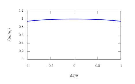
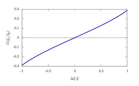
Figure 1: The functions $\widetilde{A}(\widehat{q}_{z}/\widehat{q}_{y})$ and $G(\widehat{q}_{z}/\widehat{q}_{y})$ which control the medium-induced branching rates in an anisotropic plasma are plotted as functions of the medium anisotropy $\Delta\widehat{q}/\hat{q}$, where $\Delta\widehat{q}=\widehat{q}_{z}-\widehat{q}_{y}$ and $\hat{q}=\widehat{q}_{z}+\widehat{q}_{y}$.

The splitting functions which carry an upper label 0 are the only ones to matter in the case of an isotropic medium. They have the following expressions:

$$\mathcal{F}^{0}_{z\rightarrow z}(\zeta) \,=\mathcal{F}^{0}_{y\rightarrow y}(\zeta)=\frac{1}{2}\left(\frac{1-\zeta}{\zeta}+\frac{2\zeta}{1-\zeta}+\zeta(1-\zeta),\right)$$

$$\mathcal{F}^{0}_{z\rightarrow y}(\zeta) \,=\mathcal{F}^{0}_{y\rightarrow z}(\zeta)=\frac{1}{2}\left(\zeta(1-\zeta)+\frac{1-\zeta}{\zeta}\right).$$ (61)

For an anisotropic medium, there are additional contributions which involve the splitting functions carrying the upper index 1; these read

$$\mathcal{F}^{1}_{z\rightarrow z}(\zeta) \,=\mathcal{F}^{1}_{y\rightarrow y}(\zeta)=\frac{1}{2}\left(\frac{1-\zeta}{\zeta}+\zeta(1-\zeta)\right)$$

$$\mathcal{F}^{1}_{z\rightarrow y}(\zeta) \,=\mathcal{F}^{1}_{y\rightarrow z}(\zeta)=\frac{1}{2}\left(\frac{1-\zeta}{\zeta}-\zeta(1-\zeta)\right).$$ (62)

Using the above expressions, it is easily to check that the total branching rate, averaged over the polarisations and summed over the final ones, takes the form

$$\frac{d\mathcal{P}}{d\zeta dt}\,\equiv\,\frac{1}{2}\sum_{\lambda_{a,b}=y,z}\frac{d\mathcal{P}_{a\rightarrow b}}{d\zeta dt}={\bar{\alpha}_{s}}\frac{(\widehat{q}_{y}\widehat{q}_{z})^{1/4}}{\sqrt{2\omega}}A(\widehat{q}_{z}/\widehat{q}_{y})\,\gamma(\zeta)\mathcal{F}(\zeta),$$ (63)

were $\mathcal{F}(\zeta)$ is the unpolarised DGLAP splitting function:

$$\mathcal{F}(\zeta)\,=\,\frac{1-\zeta}{\zeta}+\frac{\zeta}{1-\zeta}+\zeta(1-\zeta).$$ (64)

Notice that the function $A(\widehat{q}_{z}/\widehat{q}_{y})$ characterises the strength of the total branching rate, whereas the function $G(\widehat{q}_{z}/\widehat{q}_{y})$ has disappeared after summing over polarisations — this function only matters for the polarisation flip at the splitting vertices.

As a check, let us verify that, using the above, we recover the well-known result for the BDMPS-Z branching rate for an unpolarised parton propagating through an isotropic medium: when $\widehat{q}_{z}=\widehat{q}_{y}=\hat{q}/2$ (and hence $A=1$ and $G=0$), one indeed finds the expected result

$$\frac{1}{2}\,\frac{d\mathcal{P}_{z\rightarrow z}+d\mathcal{P}_{y\rightarrow z}}{d\zeta dt}\,=\,\frac{1}{2}\,\frac{d\mathcal{P}_{y\rightarrow y}+d\mathcal{P}_{z\rightarrow y}}{d\zeta dt}\,=\,\frac{\bar{\alpha}_{s}}{4}\,\sqrt{\frac{\hat{q}}{\omega}}\,\gamma(\zeta)\mathcal{F}(\zeta),$$ (65)

which in particular is independent of the polarisation of the (measured) daughter gluon.

One important aspect of the splitting rates in Eqs. (54)–(57) is the fact that, unlike the familiar law for bremsstrahlung in the vacuum, they depend not only upon the splitting fraction $\zeta$, but also upon the energy $\omega$ of the parent parton: the medium-induced branching probability increases like $1/\sqrt{\omega}$ with decreasing $\omega$. This feature is of course well known for the case of an isotropic medium, where it has important consequences (notably, in relation with multiple branching; see e.g. Baier:2000sb ; Blaizot:2012fh ; Blaizot:2013hx ; Blaizot:2013vha ; Kurkela:2014tla ), that we briefly recall now. Its additional implications for the case where the plasma is anisotropic will be thoroughly discussed in the remaining part of the paper.

So, let us consider the branching rate for an unpolarised parent parton in an isotropic medium, cf. Eqs. (63) and (65). After integrating this rate over all times $0<t<L$, with $L$ the medium size available to the parent parton, one finds

$$\frac{d\mathcal{P}}{d\zeta}\,=\,\bar{\alpha}_{s}\frac{L}{t_{f}(\omega,\zeta)}\,\mathcal{F}(\zeta)\qquad\mbox{with}\qquad t_{f}(\omega,\zeta)\equiv\sqrt{\frac{4\zeta(1-\zeta)\omega}{\hat{q}[1-\zeta(1-\zeta)]}}\,.$$ (66)

The quantity $\zeta(d\mathcal{P}/d\zeta)$ can be interpreted as the probability for having a single branching with splitting fraction $\zeta<1/2$. When this quantity becomes of order one or larger, the effects of multiple branching become important and our formalism must be extended to account for them. According to Eq. (66), this happens when $\zeta(1-\zeta)\omega\lesssim\omega_{\textrm{br}}\equiv\bar{\alpha}_{s}^{2}\omega_{c}$, where we recall that $\omega_{c}=\hat{q}L^{2}/2$. This condition is satisfied by two types of emissions: (i) very asymmetric emissions with $\zeta\ll 1$ by a parent parton with generic energy $\omega$, or (ii) quasi-democratic emissions with generic values of $\zeta$ (say, $\zeta\sim 1/2$), but such that the parent parton itself is sufficiently soft: $\omega\lesssim\omega_{\textrm{br}}$. Case (i) typically applies to the successive emissions of “primary” gluons by the leading parton (whose initial energy $E$ can be very large, even larger than $\omega_{c}$). These primary gluons have typical energies $\omega\lesssim\omega_{\textrm{br}}$, since for such energies, their emission probability is of order one.

After being emitted, the primary gluons are bound to split further, mostly via democratic branchings, and thus transmit their energy to a myriad of even softer gluons. The typical interval $\Delta t$ between two such branchings can be estimated by replacing $L\to\Delta t$ in Eq. (66): the probability $\zeta(d\mathcal{P}/d\zeta)$ becomes $\sim\mathcal{O}{(1)}$ when $\Delta t\sim t_{f}(\omega)/\bar{\alpha}_{s}$, which is much smaller than $L$ for low enough $\omega\ll\omega_{\textrm{br}}$. These “democratic cascades” are expected to stop when the gluon energies become as small as the typical energies of the plasma constituents (say, their temperature $T$ for a medium in thermal equilibrium) or as the Bethe-Heitler energy $\omega_{\rm BH}$, which corresponds to emissions with formation times of the order of the mean free path.

In Sect. 4, this picture of jet evolution via multiple branching will be generalised to include anisotropy effects and to keep trace of the parton polarisations.

3.4 Polarisation distribution after one splitting: a qualitative discussion

To get more intuition for the formalism developed so far, let us compute the transmission of polarisation via a single gluon branching. Specifically, we shall assume that the parent gluon has probability $p$ of being polarized in the $z$ direction and hence probability $1-p$ of being polarized in the $y$ direction. We are interested in the probility $p^{\prime}$ for an emitted daughter parton with splitting fraction $\zeta$ to be polarized in the $z$ direction. This is given by

$$p^{\prime}=\frac{p\,\mathcal{P}_{z\rightarrow z}+(1-p)\mathcal{P}_{y\rightarrow z}}{p\left(\mathcal{P}_{z\rightarrow z}+\mathcal{P}_{z\rightarrow y}\right)+(1-p)\left(\mathcal{P}_{y\rightarrow z}+\mathcal{P}_{y\rightarrow y}\right)}$$ (67)

where $\mathcal{P}_{z\rightarrow z}=d\mathcal{P}_{z\rightarrow z}/d\zeta dt$ etc is a shorthand for the splitting rates introduced in Eqs. (54)–(57). Notice that the dependence upon the energy $\omega$ of the parent parton disappears in the ratio. Hence, the r.h.s. of Eq. (67) merely depends upon the splitting fraction $\zeta$.

For more clarity, we first analyze the case of an isotropic medium with $\widehat{q}_{z}=\widehat{q}_{y}=\hat{q}/2$. In that case, the dependence upon $\hat{q}$ drops out in the ratio and we are left with

$$p^{\prime}-\frac{1}{2}=h(\zeta)\left(p-\frac{1}{2}\right)$$ (68)

where

$$\begin{split}h(\zeta)\equiv\frac{\zeta^{2}}{(1-\zeta)^{2}+\zeta^{2}+\zeta^{2}(1-\zeta)^{2}}\end{split}$$ (69)

We immediately see that for $p=1/2$, i.e. an unpolarised initial gluon, the emitted gluon is also unpolarised, $p^{\prime}=1/2.$ Importantly, $0\leq h(\zeta)\leq 1$ for all $0\leq\zeta\leq 1$. Therefore, in an isotropic medium, the net polarisation reduces with each splitting. After multiple splitting we therefore expect the net polarisation of the initial gluon to have gone away. Furthermore, $h(\zeta=1)=1$, so when the daughter parton carries all of the energy fraction of the mother parton, we have $p^{\prime}=p$. Similarly, $h(\zeta=0)=0$ so that a soft parton has no knowledge of the polarisation of the mother parton and is unpolarised in an isotropic medium.

We now turn to the case of an anisotropic medium, for which we find

$$p^{\prime}-\frac{1}{2}=\frac{\zeta^{2}(p-1/2)+\frac{1}{2}\,G(\widehat{q}_{z}/\widehat{q}_{y})(1-\zeta)^{2}}{(1-\zeta)^{2}+\zeta^{2}+\zeta^{2}(1-\zeta)^{2}+2\,G(\widehat{q}_{z}/\widehat{q}_{y})\,(p-1/2)\zeta^{2}(1-\zeta^{2})}$$ (70)

This equation becomes more intuitive if we assume that the net initial polarization is small, $p-1/2\ll 1$, and/or the medium is only slightly anisotropic, $\Delta\widehat{q}\ll\hat{q}$, so that we can drop the term proportional to $(p-1/2)G$ in the denominator. Then

$$p^{\prime}-\frac{1}{2}=h(\zeta)\left(p-\frac{1}{2}\right)+g(\zeta)\,\frac{1}{2}\,G(\widehat{q}_{z}/\widehat{q}_{y}).$$ (71)

where

$$g(\zeta)\equiv\frac{(1-\zeta)^{2}}{(1-\zeta)^{2}+\zeta^{2}(1-\zeta)^{2}+\zeta^{2}}=h(1-\zeta).$$ (72)

The second term on the right hand side of Eq. (71) is a source term that increases polarisation in the $z$ direction (assuming that $G>0$). It is independent of the polarisation of the mother parton.

In Eq. (71) we have two competing effects. The term $h(\zeta)\left(p-\frac{1}{2}\right)$, which is also present in an isotropic medium, tends to reduce the net polarisation. The other term proportional to $G(\widehat{q}_{z}/\widehat{q}_{y})$ tends to align the polarisation of the daughter gluon with the $z$ direction. When the daughter parton carries nearly all of the energy of its parent, $\zeta\rightarrow 1$, we find

$$p^{\prime}-\frac{1}{2}\simeq p-\frac{1}{2}+(1-\zeta)^{2}\frac{1}{2}\,G(\widehat{q}_{z}/\widehat{q}_{y}),$$ (73)

where the source term $\propto(1-\zeta)^{2}G$ is very small and should strictly speaking be discarded. Thus the daughter parton nearly retains the polarisation of the mother parton. In the opposite situation where the measured daughter parton is soft $\zeta\rightarrow 0$, we obtain

$$p^{\prime}-\frac{1}{2}\simeq\zeta^{2}\left(p-\frac{1}{2}\right)+\frac{1}{2}\,G(\widehat{q}_{z}/\widehat{q}_{y}).$$ (74)

This time, it is the first term $\propto\zeta^{2}$ which can be discarded, hence the polarisation of the soft daughter gluon is nearly independent of that of its parent and it is fully driven by the anisotropy of the medium: when $G>0$, its polarisation is aligned with the $z$ axis.

4 Jet evolution in an anisotropic medium

So far we have considered a single splitting in an anisotropic medium. Yet, our focus is on the relatively soft emissions with formation times $t_{f}\ll L$, for which the effects of multiple branching are expected to be important. Hence, in order to understand what a jet looks like after traversing an anisotropic plasma, we need to allow for multiple splittings. We will do this by solving evolution equations for the jet. These are rate equations — i.e. kinetic equations involving gain and loss terms — with the rates given by the probabilities for one splitting per unit time, as shown in Eqs. (54)–(57).

We want to track how the polarisation of jet partons at energy fraction $\xi=\omega/E$ changes with time. Here $\omega$ is the energy of a parton and $E$ is the energy of the initial parton that seeds the jet. As before, we assume that the leading parton moves along the $x$ axis (so, it is orthogonal to the collision axis $z$), that the jet involves only gluons, and that $\widehat{q}_{y}$ and $\widehat{q}_{z}$ are constant throughout the plasma — albeit generally different from each other. As discussed at the beginning of Sect. 3, our approach is strictly valid for parton energies within the range $\omega_{\rm BH}\ll\omega\ll\omega_{c}$, so we shall not track the very soft gluons with $\omega\lesssim\omega_{\rm BH}$, which propagate at large angles.

A crucial assumption here is that all jet partons move roughly collinearly. This is needed in order for the plane transverse to the direction of motion to be the same for all jet partons, including the softest ones. That allows us to describe the polarisation of all partons using fixed directions $y$ and $z$. This assumption is justified so long as the energies of the jet partons are much larger than the transverse momenta they acquire via collisions in the medium. Roughly speaking, the condition reads $\omega\gg\sqrt{\hat{q}L}$ with $\hat{q}\equiv\widehat{q}_{y}+\widehat{q}_{z}$, but this condition gets modified for the sufficiently soft gluons, whose lifetime (between successive splittings) is smaller than $L$ (see below).

4.1 Rate equations for medium-induced emissions of polarised gluons

Given the structure of Eqs. (54)–(57), it is convenient to define a rescaled time variable, which is dimensionless:

$$\tau\equiv\bar{\alpha}_{s}\frac{(\widehat{q}_{z}\widehat{q}_{y})^{1/4}}{\sqrt{2E}}A(\widehat{q}_{z}/\widehat{q}_{y})\,t$$ (75)

We shall use the notation $\tau_{L}$ for the maximum value of this variable, corresponding to $t=L$. To gain more intuition for the maximum value, let us notice that, in the case of an isotropic plasma ($\widehat{q}_{z}=\widehat{q}_{y}\equiv\hat{q}/2$),

$$\tau_{L}\,=\bar{\alpha}_{s}\sqrt{\frac{\hat{q}}{4E}}\,L=\sqrt{\frac{\omega_{\textrm{br}}}{2E}}\qquad\mbox{and}\qquad\frac{\tau_{L}}{\sqrt{\xi}}=\sqrt{\frac{\omega_{\textrm{br}}}{2\omega}}\,,$$ (76)

where $\omega=\xi E$ and we recall that $\omega_{\textrm{br}}=\bar{\alpha}_{s}^{2}\omega_{c}=\bar{\alpha}_{s}^{2}\hat{q}L^{2}/2$. From the discussion following Eq. (66), we recall that multiple branchings become important when $\omega\lesssim\omega_{\textrm{br}}$. Therefore the most interesting physical regime for us here corresponds to the case where $1\gg\tau_{L}\gtrsim\sqrt{\xi}\gg\xi$. The condition $\tau_{L}\ll 1$ ensures that $E\gg\omega_{\textrm{br}}$, so the leading parton survives in the final jet, after crossing the medium (it does not suffer a democratic branching itself). The condition $\tau_{L}\gtrsim\sqrt{\xi}$ means that we concentrate on gluon emissions which are sufficiently soft ($\omega=\xi E\lesssim\omega_{\textrm{br}}$) to be sensitive to multiple branching. They can be either soft ($\zeta\ll 1$) primary emissions by the leading parton, or quasi-democratic branchings ($\zeta\sim 1/2$) of the primary gluons.

In terms of this new time variable, the medium-induced branching rates take a more compact form, e.g.

$$\begin{split}\frac{d\mathcal{P}_{z\rightarrow z}}{d\zeta d\tau}=\frac{\gamma(\zeta)}{\sqrt{\xi}}\left[\mathcal{F}^{0}_{z\rightarrow z}(\zeta)+G(\widehat{q}_{z}/\widehat{q}_{y})\mathcal{F}^{1}_{z\rightarrow z}(\zeta)\right].\end{split}$$ (77)

We observe once again that the branching rate depends not only upon the splitting fraction $\zeta$ but also upon the energy fraction $\xi$ of the parent gluon.

These branching rates are the main ingredients of the equations describing the time evolution of the energy distributions of gluons with a given polarisation state, $\lambda=y$ or $\lambda=z$. These evolution equations (a.k.a. rate equations) are conveniently written for the respective spectra,

$$D_{y}\equiv\xi\frac{dN_{y}}{d\xi}\,,\qquad D_{z}\equiv\xi\frac{dN_{z}}{d\xi}\,,$$ (78)

where $N_{\lambda}(\xi)$ is the number of jet constituents with polarisation $\lambda$ and energy fraction $\xi$. By following standard techniques (e.g. the method of the generating functional described in Blaizot:2013vha ), one deduces the two following coupled equations for $D_{y}$ and $D_{z}$:

$$\begin{split}\frac{dD_{y}(\xi,\tau)}{d\tau}&=\int_{\xi}^{1}d\zeta\;\mathcal{K}_{z\rightarrow y}(\zeta)\,\sqrt{\frac{\zeta}{\xi}}\,D_{z}\left(\frac{\xi}{\zeta},\tau\right)+\int_{\xi}^{1}d\zeta\;\mathcal{K}_{y\rightarrow y}(\zeta)\,\sqrt{\frac{\zeta}{\xi}}\,D_{y}\left(\frac{\xi}{\zeta},\tau\right)\\ &-\frac{1}{2}\int_{0}^{1}d\zeta\;\Big{[}\mathcal{K}_{y\rightarrow z}(\zeta)+\mathcal{K}_{y\rightarrow y}(\zeta)\Big{]}\,\frac{1}{\sqrt{\xi}}\,D_{y}(\xi,\tau),\end{split}$$ (79)

and

$$\begin{split}\frac{dD_{z}(\xi,\tau)}{d\tau}&=\int_{\xi}^{1}d\zeta\;\mathcal{K}_{z\rightarrow z}(\zeta)\,\sqrt{\frac{\zeta}{\xi}}\,D_{z}\left(\frac{\xi}{\zeta},\tau\right)+\int_{\xi}^{1}d\zeta\;\mathcal{K}_{y\rightarrow z}(\zeta)\,\sqrt{\frac{\zeta}{\xi}}\,D_{y}\left(\frac{\xi}{\zeta},\tau\right)\\ &-\frac{1}{2}\int_{0}^{1}d\zeta\;\Big{[}\mathcal{K}_{z\rightarrow z}(\zeta)+\mathcal{K}_{z\rightarrow y}(\zeta)\Big{]}\,\frac{1}{\sqrt{\xi}}\,D_{z}(\xi,\tau).\end{split}$$ (80)

The splitting kernels $\mathcal{K}_{z\rightarrow z}(\zeta)$ etc. contain the $\zeta$–dependence of the branching rates like Eq. (77); they are defined as, e.g.

$$\mathcal{K}_{z\rightarrow z}(\zeta)\equiv\,\sqrt{\xi}\,\frac{d\mathcal{P}_{z\rightarrow z}}{d\zeta d\tau}\,={\gamma(\zeta)}\left[\mathcal{F}^{0}_{z\rightarrow z}(\zeta)+G(\widehat{q}_{z}/\widehat{q}_{y})\mathcal{F}^{1}_{z\rightarrow z}(\zeta)\right].$$ (81)

These equations have a familiar structure, with “gain terms” and “loss terms”. The “gain terms”, as shown in the first line of each of the two equations, represent the rate for producing a gluon $(\xi,\,\lambda)$ via the branching of a parent gluon with energy fraction $\xi^{\prime}=\xi/\zeta>\xi$ and any polarisation state $\lambda^{\prime}=y$ or $z$. The “loss terms”, as shown in the second line, describe the decay of a gluon $(\xi,\,\lambda)$ into two softer gluons with energy fractions $\zeta\xi$ and $(1-\zeta)\xi$ and arbitrary polarisation states. The integrals for the gain terms are restricted to $\zeta>\xi$ because of the constraint ${\xi}/{\zeta}\leq 1$ on the energy fraction of the parent gluon. The factor $1/2$ in front of the loss terms is needed to avoid double counting. Its origin is a bit subtle, so it is worth showing a more detailed argument.

Recall that a branching rate like $\mathcal{K}_{z\rightarrow z}$ refers to the process where, for a parent gluon with $\lambda=z$, the daughter gluon with splitting fraction $\zeta$ has polarisation $z$ independently of the polarisation state of the other daughter gluon, with splitting fraction $1-\zeta$. Hence, $\mathcal{K}_{z\rightarrow z}(\zeta)=\mathcal{K}_{z\rightarrow zz}(\zeta)+\mathcal{K}_{z\rightarrow zy}(\zeta)$ in obvious notations. Similarly, $\mathcal{K}_{z\rightarrow y}(\zeta)=\mathcal{K}_{z\rightarrow yz}(\zeta)+\mathcal{K}_{z\rightarrow yy}(\zeta)$. Now, in the loss term in Eq. (80), $\zeta$ is a dummy variable which can take any value between 0 and 1. The decays where both daughter partons are in a same polarisation state, i.e. $\mathcal{K}_{z\rightarrow zz}(\zeta)$ and $\mathcal{K}_{z\rightarrow yy}(\zeta)$, are symmetric under the exchange of the daughter gluons, since the respective rates are symmetric under $\zeta\to 1-\zeta$ (recall Eqs. (34) and (37)). Clearly, such processes would be counted twice when integrating over all values of $\zeta$. As for the remaining processes where the daughter gluons have different polarisation states, their rates get interchanged when $\zeta\to 1-\zeta$; that is, $\mathcal{K}_{z\rightarrow zy}(1-\zeta)=\mathcal{K}_{z\rightarrow yz}(\zeta)$, cf. Eqs. (35) and (36). So, these processes too would be counted twice after integrating over $\zeta$.

In order to make contact with the known equations for the case of an isotropic plasma and for unpolarised gluons, it is convenient to use the following linear combinations of $D_{y}$ and $D_{z}$:

$$D_{\mathrm{tot}}\equiv D_{y}+D_{z},\qquad\mbox{and}\qquad\widetilde{D}\equiv D_{z}-D_{y}.$$ (82)

$D_{\mathrm{tot}}$ is the total spectrum for gluons and $\widetilde{D}$ is the jet polarisation. Using Eqs. (79) and (80), it is straightforward to deduce the corresponding equations for $D_{\mathrm{tot}}$ and $\widetilde{D}$. The general equations are not very illuminating (we include them in Appendix B, where we also check their isotropic limit), but they become more transparent — and also better suited for constructing (analytic and numerical) solutions — in the limit in which we keep only the singular behaviour of the branching rates near $\zeta=0$ and $\zeta=1$. That is, we neglect the contributions proportional to $\zeta(1-\zeta)$ in Eqs. (3.3)–(3.3) and also in the structure (58) of the splitting kernel $\gamma(\zeta)$. This approximation, which is similar to that performed in Blaizot:2013hx for the case of an isotropic medium, keeps all the salient features of the branching process, which is indeed driven by its singular points at $\zeta=0$ and $\zeta=1$. For an isotropic medium, this has been explicitly checked by comparing the solutions numerically obtained with the two types of kernel (exact and approximate) Fister:2014zxa ; Blaizot:2015jea . With this simplification, the equations obeyed by $D_{\mathrm{tot}}$ and $\tilde{D}$ take particularly suggestive forms:

$$\frac{dD_{\mathrm{tot}}(\xi,\tau)}{d\tau}=\int_{\xi}^{1}d\zeta\;\mathcal{K}_{0}(\zeta)\sqrt{\frac{\zeta}{\xi}}\,D_{\mathrm{tot}}\left(\frac{\xi}{\zeta},\tau\right)-\int_{0}^{1}d\zeta\;\mathcal{K}_{0}(\zeta)\,\frac{\zeta}{\sqrt{\xi}}\,D_{\mathrm{tot}}(\xi,\tau)$$ (83)

and

$$\begin{split}\frac{d\widetilde{D}(\xi,\tau)}{d\tau}&=\int_{\xi}^{1}d\zeta\;\mathcal{M}_{0}(\zeta)\,\sqrt{\frac{\zeta}{\xi}}\,\widetilde{D}\left(\frac{\xi}{\zeta},\tau\right)-\int_{0}^{1}d\zeta\;\mathcal{K}_{0}(\zeta)\,\frac{\zeta}{\sqrt{\xi}}\,\widetilde{D}(\xi,\tau)\\ &+\int_{\xi}^{1}d\zeta\;\mathcal{L}_{0}(\zeta)\,\sqrt{\frac{\zeta}{\xi}}\,D_{\mathrm{tot}}\left(\frac{\xi}{\zeta},\tau\right).\end{split}$$ (84)

with the new kernels (see Appendix B for details)

$$\mathcal{K}_{0}(\zeta)\equiv\frac{1}{\zeta^{3/2}(1-\zeta)^{3/2}},\qquad\mathcal{L}_{0}(\zeta)\equiv\frac{(1-\zeta)^{1/2}}{\zeta^{3/2}}\,G(\widehat{q}_{z}/\widehat{q}_{y}),\qquad\mathcal{M}_{0}(\zeta)\equiv\frac{\zeta^{1/2}}{(1-\zeta)^{3/2}}.$$ (85)

These equations have an intuitive interpretation. The evolution equation for the total number of partons $D_{\mathrm{tot}}$ takes exactly the same form as for an isotropic medium Blaizot:2013hx ; Blaizot:2013vha . This “coincidence” is not an exact property — it only holds within our present approximations, which neglected the non-singular contributions to the splitting functions. (The general equation, as shown in Eq. (112), is more complicated and involves contributions proportional to $\widetilde{D}$.) The exact solution to this equation is known in analytic form Blaizot:2013hx and this will be useful for what follows.

The equation (84) obeyed by the polarised distribution $\widetilde{D}$ is new and has an interesting structure: besides a gain term and a loss term, with kernels $\mathcal{M}_{0}(\zeta)$ and $\mathcal{K}_{0}(\zeta)$, respectively, it also features a source term, proportional to the total parton distribution $D_{\mathrm{tot}}$, which is non-zero only in the presence of anisotropy. Indeed, its kernel $\mathcal{L}_{0}(\zeta)$ is proportional to the function $G(\widehat{q}_{z}/\widehat{q}_{y})$ which would vanish for an isotropic plasma, cf. Eq. (59). This demonstrates that, in an anisotropic medium, non-trivial polarisation can be generated via medium-induced gluon branchings, independently of the polarisation of the parent gluons.

This is in agreement with our previous discussion of a single splitting in Sect. 3.4: the source term in Eq. (84) is analogous to the second piece, proportional to $G(\widehat{q}_{z}/\widehat{q}_{y})$, in the r.h.s. of Eq. (71). In fact, one can recognise similar properties in both cases. The kernel $g(\zeta)$ in Eq. (71) vanishes like $(1-\zeta)^{2}$ as $\zeta\rightarrow 1$, whereas the corresponding kernel $\mathcal{L}_{0}(\zeta)$ in Eq. (84) is suppressed by $(1-\zeta)^{2}$ relative to the isotropic functions $\mathcal{K}_{0}(\zeta)$ and $\mathcal{M}_{0}(\zeta)$. This reflects the fact that a daughter parton carrying nearly all of the energy of its parent parton does not “feel” the anisotropy of the medium — rather, it retains the polarisation of the parent.

Furthermore, the gain term on the r.h.s. of Eq. (84), with kernel $\mathcal{M}_{0}(\zeta)$, show how polarisation gets transmitted from the parent parton to the daughter parton with splitting fraction $\zeta$. It is analogous to the first term on the right hand side in Eq. (71) for a single splitting. Like in that case, the respective kernel is suppressed by $\zeta^{2}$ in the soft limit $\zeta\rightarrow 0$ (soft gluons do not “know” about the polarisation of their parents). Finally, the loss term on the r.h.s of Eq. (84) describes the decay of partons carrying polarisation. As their total decay rate is (to our order of approximation) independent of their polarisation, the respective kernel is the unpolarised function $\mathcal{K}_{0}(\zeta)$ — the same as in Eq. (83).

4.2 A Green’s function for the polarised gluon distribution

In what follows, we shall solve the rate equations (83) and (84) with the initial condition that, at time $\tau=0$, the jet consists of a single gluon (the “leading parton”) which is unpolarised:

$$D_{\mathrm{tot}}(\xi,\tau=0)=\delta(1-\xi)\qquad\mbox{and}\qquad\widetilde{D}(\xi,\tau=0)=0.$$ (86)

The corresponding solution for $D_{\mathrm{tot}}$ is known in analytic form and reads Blaizot:2013hx ; Blaizot:2015jea

$$D_{\mathrm{tot}}(\xi,\tau)=\frac{\tau}{\sqrt{\xi}(1-\xi)^{3/2}}\,e^{-\pi\tau^{2}/(1-\xi)}\,.$$ (87)

For small $\tau$ and $\xi$ close to 1, this exhibits a pronounced peak at $1-\xi\lesssim\tau^{2}$ which describes the leading parton. The width of this peak reflects the fact that the energy loss by the leading parton, namely $E(1-\xi)\sim E\tau^{2}\sim\bar{\alpha}_{s}^{2}\hat{q}t^{2}$, is associated with the radiation of soft gluons. For $\xi\ll 1$, the full spectrum in presence of multiple branching, $D_{\mathrm{tot}}\simeq{\tau}/{\sqrt{\xi}}$, is formally the same as the spectrum that would be created via a single emission by the leading parton, cf. Eq. (66). This reflects the turbulent nature of the democratic gluon cascades Blaizot:2013hx . In particular, the power-law spectrum $1/\sqrt{\xi}$ is a fixed point of the rate equation (83): the gain and loss terms in its r.h.s. exactly cancel each other for this particular spectrum.

The knowledge of the exact solution (87) for the total spectrum allows us to deduce the corresponding solution $D_{\mathrm{tot}}$ for the polarised distribution $\widetilde{D}$ without too much effort. To that aim, it is convenient to first consider the homogeneous version of Eq. (84), that is, the equation obtained after removing the source term in the second line of (84). For more clarity, we denote the respective solution as $\widetilde{D}_{0}(\xi,\tau)$; this obeys the homogeneous equation

$$\begin{split}\frac{d\widetilde{D}_{0}(\xi,\tau)}{d\tau}=\int_{\xi}^{1}d\zeta\;\mathcal{M}_{0}(\zeta)\,\sqrt{\frac{\zeta}{\xi}}\,\widetilde{D}_{0}\left(\frac{\xi}{\zeta},\tau\right)-\int_{0}^{1}d\zeta\;\mathcal{K}_{0}(\zeta)\,\frac{\zeta}{\sqrt{\xi}}\,\widetilde{D}_{0}(\xi,\tau),\end{split}$$ (88)

with the initial condition $\widetilde{D}_{0}(\xi,\tau=0)=\delta(1-\xi)$. The only difference w.r.t. Eq. (83) for $D_{\mathrm{tot}}$ refers to the kernel $\mathcal{M}_{0}(\zeta)$ for the gain term, which satisfies $\mathcal{M}_{0}(\zeta)=\zeta^{2}\mathcal{K}_{0}(\zeta)$ (cf. Eq. (85)). It is then easy to check that the respective solutions are related in the same way, that is,

$$\widetilde{D}_{0}(\xi,\tau)\,=\,\xi^{2}D_{\mathrm{tot}}(\xi,\tau)\,=\,\frac{\xi^{3/2}\,\tau}{(1-\xi)^{3/2}}\,e^{-\pi\tau^{2}/(1-\xi)}\,.$$ (89)

This can be demonstrated by inserting $\widetilde{D}_{0}\equiv\xi^{2}\widetilde{D}_{1}$ within Eq. (88); one then finds that $\widetilde{D}_{1}$ obeys the same equation as $D_{\mathrm{tot}}$, i.e. Eq. (83), with the initial condition $\widetilde{D}_{1}(\xi,\tau=0)=\delta(1-\xi)$.

Here, we merely use Eq. (88) as an auxiliary equation, but in fact, this equation has an interesting interpretation, which is more transparent in the case of an isotropic plasma. In that case, Eq. (88) describes the transmission of polarisation from the leading parton to the partons in the cascade via successive branchings. Its solution (89) represents the polarised gluon distribution created by a leading gluon with initial polarisation along the $z$ axis ($D_{z}(\xi,\tau=0)=\delta(1-\xi)$ and $D_{y}(\xi,\tau=0)=0$). For $\xi\simeq 1$, Eq. (89) is very similar to the unpolarised distribution (87); this shows that the leading parton essentially preserves its initial polarisation so long as it survives in the medium (i.e. for $\tau\ll 1$). On the other hand, for the much softer modes with $\xi\ll 1$, $\widetilde{D}_{0}(\xi,\tau)$ is suppressed by $\xi^{2}$ compared to $D_{\mathrm{tot}}(\xi,\tau)$, meaning that the net polarisation is negligible. This is of course consistent with the fact that soft gluons cannot inherit the polarisation of their parents. These considerations are illustrated in the left panel of Fig. 2, where we have plotted the two functions $D_{\mathrm{tot}}(\xi,\tau)$ and $\widetilde{D}_{0}(\xi,\tau)$.

The above discussion shows that the only way to generate a net polarisation for the soft gluons is through the effects of anisotropy, as encoded in the source term in Eq. (84). Using the above solution for $\widetilde{D}_{0}(\xi,\tau)$, one can construct the Green’s function $G(\xi,\xi_{1},\tau)$ which permits to solve the inhomogeneous equation (84) for an arbitrary source term. This Green’s function obeys the sourceless equation, that is,

$$\begin{split}\frac{dG(\xi,\xi_{1},\tau)}{d\tau}=\int_{\xi}^{1}d\zeta\;\mathcal{M}_{0}(\zeta)\,\sqrt{\frac{\zeta}{\xi}}\,G\left(\frac{\xi}{\zeta},\xi_{1},\tau\right)-\int_{0}^{1}d\zeta\;\mathcal{K}_{0}(\zeta)\,\frac{\zeta}{\sqrt{\xi}}\,G(\xi,\xi_{1},\tau),\end{split}$$ (90)

with the initial condition

$$G(\xi,\xi_{1},\tau=0)\,=\,\delta(\xi-\xi_{1})\,.$$ (91)

Comparing Eqs. (90) and (88), one immediately sees that

$$G(\xi,\xi_{1},\tau)\,=\,\frac{\theta(\xi_{1}-\xi)}{\xi_{1}}\,\widetilde{D}_{0}\left(\frac{\xi}{\xi_{1}},\frac{\tau}{\sqrt{\xi_{1}}}\right).$$ (92)

Notice the $\theta$–function in the structure of $G(\xi,\xi_{1},\tau)$: it shows that the integral over $\zeta$ in the gain term in Eq. (90) is truly restricted to $\zeta>\xi/\xi_{1}$. After also using (89) and(87), one finds

$$G(\xi,\xi_{1},\tau) \,=\,\frac{\theta(\xi_{1}-\xi)}{\xi_{1}}\left(\frac{\xi}{\xi_{1}}\right)^{2}D_{\mathrm{tot}}\left(\frac{\xi}{\xi_{1}},\frac{\tau}{\sqrt{\xi_{1}}}\right)$$

$$\,=\,\theta(\xi_{1}-\xi)\left(\frac{\xi}{\xi_{1}(\xi_{1}-\xi)}\right)^{3/2}\tau\,e^{-\pi\tau^{2}/(\xi_{1}-\xi)}\,.$$ (93)

We are finally in a position to solve the inhomogeneous Eq. (84) with vanishing initial condition. The solution can be expressed via the Green’s function as

$$\widetilde{D}(\xi,\tau)=\int_{\xi}^{1}d\xi_{1}\;\int_{0}^{\tau}d\tau_{1}\,G(\xi,\xi_{1},\tau-\tau_{1})I(\xi_{1},\tau_{1}),$$ (94)

with $I(\xi_{1},\tau_{1})$ the source term in the r.h.s. of Eq. (84), that is,

$$I(\xi_{1},\tau_{1})=\int_{\xi_{1}}^{1}d\zeta\;\mathcal{L}_{0}(\zeta)\,\sqrt{\frac{\zeta}{\xi_{1}}}\,D_{\mathrm{tot}}\left(\frac{\xi_{1}}{\zeta},\tau_{1}\right).$$ (95)

This source term is non-local in energy, since associated with radiation — polarised gluons with energy fraction $\xi_{1}$ are produced via the decay of gluons with any polarisation and with larger energy fractions ${\xi_{1}}/{\zeta}$, for any $1>\zeta>\xi_{1}$ —, but is local in time, because of our assumption that medium-induced emissions are quasi-instantaneous. The ensuing convolution with the Green’s function in Eq. (94) shows how the net polarisation of gluons with energy fraction $\xi_{1}$ created at time $\tau_{1}$ propagates (via successive branchings) into the measured bin at $\xi$ at the measurement time $\tau>\tau_{1}$.

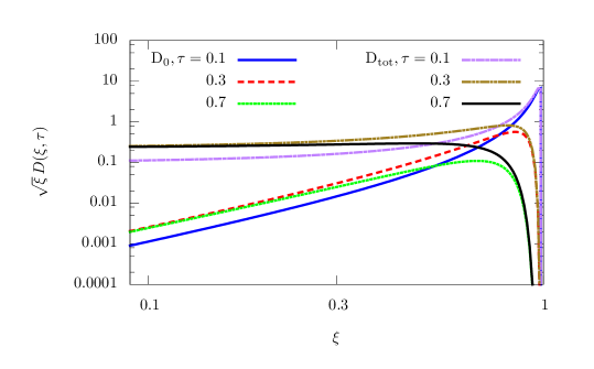
Figure 2: Left: The total (unpolarised) gluon distribution $D_{\mathrm{tot}}(\xi,\tau)$ (cf. Eq. (87)) and the polarised distribution $\widetilde{D}_{0}(\xi,\tau)$ that would be created in an isotropic medium by a polarised leading gluon (cf. Eq. (89)). Both functions are multiplied by $\sqrt{\xi}$, to emphasise the emergence of the turbulent spectrum $D_{\mathrm{tot}}\propto 1/\sqrt{\xi}$ at small $\xi\lesssim\tau^{2}$. Right: The source term $I(\xi,\tau)$ responsible for inducing polarisation in an anisotropic medium, numerically computed from Eq. (96) with $G(\widehat{q}_{z}/\widehat{q}_{y})=0.3$. The solutions are shown down to very small values of $\xi$, to check the quality of the analytic approximation (97).

4.3 The polarised jet distribution

Eq. (94) with the source term (95) represents an exact but formal solution to the equation obeyed by the polarised jet distribution $\widetilde{D}(\xi,\tau)$. In order to render this solution more explicit and uncover its physical consequences, one needs to (at least, approximately) perform the remaining convolutions over $\xi_{1}$ and $\tau_{1}$, and also the integral over $\zeta$ in the expression (95) for the source term. As previously explained, we are mainly interested in the production of soft gluons with $\xi\ll 1$ at relatively small times $\tau\ll 1$, so we shall adapt our approximations to these conditions.

Let us start by simplifying the source term. Using the expression in Eq. (85) for the kernel $\mathcal{L}_{0}$ together with Eq. (87) for $D_{\mathrm{tot}}$, one finds

$$I(\xi_{1},\tau_{1})=G(\widehat{q}_{z}/\widehat{q}_{y})\int_{\xi_{1}}^{1}d\zeta\;(1-\zeta)^{1/2}\,\frac{\zeta}{\xi_{1}}\frac{\tau_{1}}{(\zeta-\xi_{1})^{3/2}}\,e^{-\pi\tau_{1}^{2}\zeta/(\zeta-\xi_{1})}\,.$$ (96)

We shall later check that, when $\xi\ll 1$, the convolution in Eq. (94) is controlled by $\xi_{1}\ll 1$ as well. On the other hand, the integral in Eq. (96) is convergent at its upper limit and hence is dominated by relatively large values $\zeta\sim 1$. Indeed the would-be pole of the integrand at $\zeta=\xi_{1}$ is regulated by the exponential, which effectively restricts the support of the integration to $\zeta-\xi_{1}\gtrsim\zeta\tau_{1}^{2}$. We can therefore neglect $\xi_{1}$ next to $\zeta$ inside the integrand, to deduce

$$\begin{split}I[\xi_{1},\tau_{1}]&\simeq G(\widehat{q}_{z}/\widehat{q}_{y})\,\frac{\tau_{1}e^{-\pi\tau_{1}^{2}}}{\xi_{1}}\int_{0}^{1}d\zeta\,\sqrt{\frac{1-\zeta}{\zeta}}=\,G(\widehat{q}_{z}/\widehat{q}_{y})\,\frac{\pi\tau_{1}e^{-\pi\tau_{1}^{2}}}{2\xi_{1}}.\end{split}$$ (97)

The final integral is indeed controlled by values of $\zeta$ in the bulk, say $\zeta\sim 1/2$, in agreement with our previous discussion. This argument also shows that the polarisation source at $\xi_{1}\ll 1$ is generated via the democratic branching of an unpolarised parent gluon which is itself soft, with energy fraction $\xi^{\prime}=\xi_{1}/\zeta\sim 2\xi_{1}$. This dominance of the democratic branchings within the source term is not a consequence of the polarised splitting function — by itself, the kernel $\mathcal{L}_{0}(\zeta)$ in Eq. (85) would rather favour very asymmetric splittings with $\zeta\ll 1$ —, but rather of the fact that the number of sources $D_{\mathrm{tot}}(\xi^{\prime},\tau_{1})$ is rapidly increasing with decreasing $\xi^{\prime}=\xi_{1}/\zeta$. Since $\xi_{1}$ itself is small, this property favours relatively large values of $\zeta$, albeit not too large — since the kernel $\mathcal{L}_{0}(\zeta)$ vanishes when $\zeta\to 1$. This competition ultimately selects intermediate values $\zeta\sim 1/2$.

In the right panel of Fig. 2, we display the results for the source term obtained via numerical integration in Eq. (96). Besides confirming the power-law increase $\propto 1/\xi_{1}$ at small $\xi_{1}\ll 1$ as analytically found in Eq. (97), these numerical results also show an interesting behaviour at larger values $\xi_{1}>0.1$: the source term is rather abruptly generated when decreasing $\xi_{1}$ below 1. This region at large $\xi_{1}$ is not covered by our previous approximation (97), yet it can be analytically understood as follows: so long as $\tau_{1}\ll 1$, a polarised distribution at $\xi_{1}\sim\mathcal{O}{(1)}$ can be generated via primary emissions by the leading parton. This direct contribution to the source term can be estimated by replacing $D_{\mathrm{tot}}\left({\xi_{1}}/{\zeta},\tau_{1}\right)\simeq\delta({\xi_{1}}/{\zeta}-1)$ within the integrand of (95), which yields

$$I(\xi_{1},\tau_{1})\,\simeq\,\xi_{1}\mathcal{L}_{0}(\xi_{1})\,=\,\sqrt{\frac{1-\xi_{1}}{\xi_{1}}}\,G(\widehat{q}_{z}/\widehat{q}_{y}).$$ (98)

This result is independent of time but truly holds only for very small times $\tau_{1}\ll 1$. Its dependence upon $\xi_{1}$ explains the shape of the curves in Fig. 2 (right) near $\xi_{1}=1$. As expected, the leading parton contribution (98) to the source term dominates at $\xi_{1}>\tau_{1}^{2}$, whereas the respective contribution (97) from democratic branchings becomes dominant at small $\xi_{1}\lesssim\tau_{1}^{2}$.

Substituting the approximate expression (97) for the source together with Eq. (4.2) for the Green’s function into Eq. (94), one finds

$$\widetilde{D}(\xi,\tau)\simeq\frac{\pi}{2}\,G(\widehat{q}_{z}/\widehat{q}_{y})\int_{\xi}^{1}d\xi_{1}\int_{0}^{\tau}d\tau_{1}\;\left(\frac{\xi}{\xi_{1}(\xi_{1}-\xi)}\right)^{3/2}(\tau-\tau_{1})\;e^{-\pi\frac{(\tau-\tau_{1})^{2}}{\xi_{1}-\xi}}\;\frac{\tau_{1}}{\xi_{1}}\,e^{-\pi\tau_{1}^{2}}\,.$$ (99)

The integrand involves a competition between the power laws $\xi_{1}^{-5/2}(\xi_{1}-\xi)^{-3/2}$, which strongly enhance the contribution from values of $\xi_{1}$ as small as possible, meaning $\xi_{1}\sim\xi$, and the exponential $\exp{\big{\{}-\pi(\tau-\tau_{1})^{2}/(\xi_{1}-\xi)\big{\}}}$, which limits the difference $\xi_{1}-\xi$ to non-zero values $\xi_{1}-\xi\gtrsim\Delta\tau^{2}$, with $\Delta\tau\equiv\tau-\tau_{1}$. Since however both $\xi_{1}$ and $\Delta\tau$ are integration variables, it seems quite clear that the maximal contribution to the integral should come from their minimal values allowed by these two constraints, namely $\Delta\tau^{2}\sim\xi_{1}-\xi\sim\xi$. Indeed, with these choices, $\xi_{1}\sim 2\xi$ is parametrically of order $\xi$, yet the exponent remains of order one, so there is no exponential suppression. These values for $\xi_{1}$ and $\Delta\tau$ are in fact correlated with each other: $\xi_{1}\sim 2\xi$ corresponds to a democratic branching and $\Delta\tau\sim\sqrt{\xi}$ is indeed the typical lifetime of a gluon with energy fraction $\xi_{1}\sim\xi$ before it undergoes such a democratic branching, as discussed after Eq. (66).

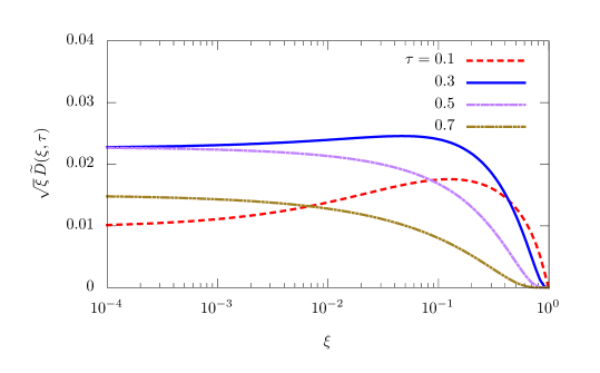
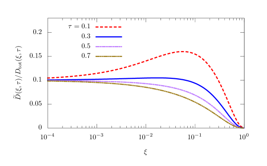
Figure 3: The polarised gluon distribution $\widetilde{D}(\xi,\tau)$ created in an anisotropic medium with $G(\widehat{q}_{z}/\widehat{q}_{y})=0.29$ by an unpolarised leading gluon. The results are obtained via numerical integration in Eq. (94) with the source term from (95) and the Green’s function (4.2). Left: $\widetilde{D}(\xi,\tau)$ is multiplied by $\sqrt{\xi}$ to emphasise the turbulent spectrum at small $\xi\ll\tau^{2}$ (cf. Eq. (4.3)). Right: The ratio between the polarised and unpolarised distributions; one observes their proportionality at small $\xi$, in agreement with (103).

The dominance of democratic branchings in the case of Eq. (99) has two well-identified physical origins: (i) the fact that the source term in Eq. (97) increases with decreasing $\xi_{1}$, and (ii) the fact that the Green’s function (4.2) is strongly suppressed for very asymmetric splittings with $\zeta\equiv\xi/\xi_{1}\ll 1$ (which in turn reflects the fact that soft splittings lose memory of the polarisation of the parent parton).

Although physically appealing, the above argument calls for an explicit mathematical proof, that we now present. To that aim, it is convenient to perform a change of integration variables, from $\tau_{1}$ and $\xi_{1}$, to $\Delta\tau=\tau-\tau_{1}$ and $v\equiv\sqrt{\xi/(\xi_{1}-\xi)}$. Then Eq. (99) becomes

$$\widetilde{D}(\xi,\tau)\simeq\frac{\pi}{\xi^{3/2}}\,G(\widehat{q}_{z}/\widehat{q}_{y})\int\limits_{\sqrt{\xi/(1-\xi)}}^{\infty}dv\left[\frac{v^{2}}{1+v^{2}}\right]^{5/2}\int_{0}^{\tau}d\Delta\tau\,\Delta\tau\,\big{(}\tau-\Delta\tau\big{)}\;e^{-\pi\frac{v^{2}\Delta\tau^{2}}{\xi}}\,e^{-\pi(\tau-\Delta\tau)^{2}}\,.$$ (100)

Since $\xi\ll 1$, one can replace ${\sqrt{\xi/(1-\xi)}}\simeq\sqrt{\xi}$ in the lower limit of the integral over $v$.

We will shortly check that this double integral is controlled by values $v\sim 1$ and $\Delta\tau\sim\sqrt{\xi}$. In order to analytically perform the integrations, it is convenient to assume that $\tau$ is even larger, namely $1\gg\tau\gg\sqrt{\xi}$. Physically, this means that we focus on polarised gluons with very low energies $\omega=\xi E\ll\omega_{\textrm{br}}$ (recall that ${\xi}\sim\tau^{2}$ corresponds to $\omega\sim\omega_{\textrm{br}}$).

Since $\tau\gg\sqrt{\xi}\sim\Delta\tau$, we can neglect $\Delta\tau$ next to $\tau$ in the above integrand and then the integral over $\Delta\tau$ becomes trivial:

$$\int_{0}^{\tau}d\Delta\tau\,\Delta\tau\,\big{(}\tau-\Delta\tau\big{)}\;e^{-\pi\frac{v^{2}\Delta\tau^{2}}{\xi}}\,e^{-\pi(\tau-\Delta\tau)^{2}}\, \simeq\,\tau\,e^{-\pi\tau^{2}}\int_{0}^{\tau}d\Delta\tau\,\Delta\tau\,e^{-\pi\frac{v^{2}\Delta\tau^{2}}{\xi}}$$

$$\,=\,\tau e^{-\pi\tau^{2}}\frac{\xi}{2\pi v^{2}}\left(1-e^{-\pi\frac{v^{2}\tau^{2}}{\xi}}\right)$$ (101)

By inserting this result into Eq. (100), one finds

$$\widetilde{D}(\xi,\tau) \,\simeq\,G(\widehat{q}_{z}/\widehat{q}_{y})\,\frac{\tau e^{-\pi\tau^{2}}}{2\sqrt{\xi}}\int\limits_{\sqrt{\xi}}^{\infty}dv\frac{v^{3}}{(1+v^{2})^{5/2}}\left(1-e^{-\pi\frac{v^{2}\tau^{2}}{\xi}}\right)$$

$$\,\simeq\,G(\widehat{q}_{z}/\widehat{q}_{y})\,\frac{\tau e^{-\pi\tau^{2}}}{2\sqrt{\xi}}\int\limits_{\sqrt{\xi}/\tau}^{\infty}dv\frac{v^{3}}{(1+v^{2})^{5/2}}\,=\,\frac{G(\widehat{q}_{z}/\widehat{q}_{y})}{3}\,\frac{\tau e^{-\pi\tau^{2}}}{\sqrt{\xi}}\Big{[}1\,+\,\mathcal{O}{(\sqrt{\xi}/\tau)}\Big{]}\,.$$ (102)

Notice that the final integral is controlled by values $v\sim 1$, as anticipated. Hence, neither the exponential within the integrand in the first line, nor the lower limit $\sqrt{\xi}/\tau$ on the integral over $v$ in the second line (that was precisely introduced by the exponential) were important for the final result. Indeed, when $\tau\gg\sqrt{\xi}$ and $v\sim 1$, the exponent $v^{2}\tau^{2}/\xi$ is large and the exponential is strongly suppressed. When $v\sim 1$, it is easy to check that the previous integral in Eq. (4.3) is indeed controlled by $\Delta\tau\sim\sqrt{\xi}$.

Remarkably, $\widetilde{D}(\xi,\tau)$ is simply proportional to $D_{\mathrm{tot}}(\xi,\tau)$ for such small values of $\xi$:

$$\frac{\widetilde{D}(\xi,\tau)}{D_{\mathrm{tot}}(\xi,\tau)}\,\simeq\,\frac{G(\widehat{q}_{z}/\widehat{q}_{y})}{3}\qquad\mbox{for}\qquad{\xi}\ll\tau^{2}.$$ (103)

Although derived here for very small energies $\omega\ll\omega_{\textrm{br}}$, we expect this relation between the polarised and the total distributions to remain qualitatively true for all the gluons affected by multiple branching — those with energies $\omega\lesssim\omega_{\textrm{br}}$, or $\xi\lesssim\tau^{2}$ (so long as $\tau\ll 1$, of course). This is confirmed by a numerical calculation of $\widetilde{D}(\xi,\tau)$ based on Eqs. (94)–(95) (that is, the numerical evaluation of a series of three convolutions), with the results displayed in Fig. 3. In this calculation, we have assumed the maximum value $G(\widehat{q}_{z}/\widehat{q}_{y})=0.29$ for the quantity which measures the effects of the anisotropy on the branching rates. (As visible in Fig. 1, this value $G=0.29$ corresponds to $\Delta\widehat{q}/\hat{q}=1$, i.e. to maximum anisotropy.) Changing the value of $G$ does not change the trends visible in Fig. 3, but only the normalisation of the curves. The proportionality relation (103) is seen to be numerically verified so long as ${\xi}\ll\tau^{2}$, while small deviations are observed when increasing $\xi$ towards $\tau^{2}$.

To summarise, we have found that, even for a jet initiated by an unpolarised leading parton, the soft gluon distribution generated via multiple branching in an anisotropic medium exhibits a net polarisation, which is proportional to the medium anisotropy (via the function $G(\widehat{q}_{z}/\widehat{q}_{y})$) and also to the total (unpolarised) distribution — in particular, it exhibits the same power-law enhancement at small $\xi\ll 1$: $\widetilde{D}\propto 1/\sqrt{\xi}$. As our calculation also shows, these remarkable features are the consequence of the fact that the polarisation is essentially built in the last few splittings — one or two quasi-democratic branchings, which are close in time and also in energy to the measurement time and the energy bin.

Said differently, the polarisation is continuously created and then washed out at each step of the democratic cascade: unlike the energy (which is a conserved quantity), it does not propagate between gluons from very different generations. Accordingly, the only reason why the polarised distribution appears to increase with time and with $1/\xi$ is because the number of its sources — the unpolarised distribution $D_{\mathrm{tot}}(\xi,\tau)$ — keeps rising so long as $\tau\ll 1$, i.e. so long as the leading parton is still “alive” and acts as a source of soft primary gluons, which regenerate the cascade.

5 Conclusions and perspectives

In this paper, we have studied the evolution of a jet propagating through an anisotropic quark-gluon plasma, with emphasis on the consequences of the anisotropy for the polarisation of the jet constituents. The physical problem we had in mind is the production of jets at central rapidities in ultrarelativistic heavy ion collisions, at RHIC and the LHC. In that context, the anisotropy is naturally generated by the rapid expansion of the medium along the collision axis, leading to a squeezed momentum distribution for the partons from the plasma. Our first observation is that the medium anisotropy leads to a difference between the jet quenching parameters — the rates for transverse momentum broadening — along the two directions transverse to the jet axis: the collision axis and a direction in the plane orthogonal to it. Within the BDMPS-Z mechanism for medium-induced gluon emissions, such an asymmetry in the transverse momentum broadening naturally leads to a modification in the parton branching rates. This modification depends upon the partons’ polarisation and thus has the potential to dynamically generate net polarisation.

In order to study this, we considered a somewhat simplified scenario, in which the plasma is weakly coupled and stationary, and the anisotropy is enforced by merely assuming different values for the relevant jet quenching parameters. Also, we considered a jet which is made only of gluons. Within this set-up, we have generalised the BDMPS-Z mechanism to the anisotropic plasma and to the branchings of gluons with definite (linear) polarisation states. Our results for the splitting rates, as shown in Eqs. (54)–(57), confirm that, due to the anisotropy, the daughter gluons can carry net polarisation even when their parent gluon was unpolarised. This effect is particularly remarkable for the emissions of soft gluons which cannot inherit the polarisation of their parent: in the absence of the anisotropy, such gluons would always be unpolarised, irrespective of the polarisation state of their parent (cf. the discussion in Sect. 3.4).

Using the polarised splitting rates in Eqs. (54)–(57), we have constructed kinetic equations which determine the time evolution of the energy and polarisation distributions among the jet constituents, Eqs. (83) and (84). They represent natural generalisations of the respective equations for an isotropic medium and unpolarised gluons Blaizot:2013vha . Like the latter, the polarized kinetic equations exhibit turbulent dynamics: the soft gluons multiply via quasi-democratic branchings, which now control both the creation of net polarisation (via the decay of unpolarised partons) and its transmission from one parton generation to the next one. This transmission however is not very efficient: it is hindered by the fact that, as alluded to above, soft gluons lose memory of the polarisation of their parents. As a result, the polarisation is both created (by the anisotropy) and washed out (via the subsequent emissions of soft gluons) quasi-locally in energy and time — that is, within just a few, successive democratic branchings. Accordingly, the net polarisation of soft gluons closely follows the evolution of the unpolarised gluon distribution: the two distributions are simply proportional to each other, with a proportionality coefficient that would vanish for an isotropic plasma, cf. Eq. (103).

These considerations also suggest that for a more realistic scenario, where the plasma anisotropy decreases with time — the momentum distributions of the plasma constituents are expected to evolve towards isotropy, as a result of elastic collisions which compete with, and eventually take over, the medium expansion Baier:2000sb —, this mechanism for generating polarisation should become less and less effective with increasing time. That said, the numerical solutions to both kinetic theory Kurkela:2015qoa ; Kurkela:2018vqr ; Du:2020dvp and (viscous) relativistic hydrodynamics Heinz:2013th ; Gale:2013da ; Luzum:2013yya ; Alqahtani:2017mhy demonstrate that, even for relatively large values of the QCD coupling, the approach towards (local) thermal equilibrium is very slow. So, it is quite plausible that, during the late stages of the jet propagation through the medium — the most important ones for its evolution via medium-induced parton branchings — the anisotropy is still sizeable and only slowly varying with time. In such a case, our general conclusions in this paper should remain valid (at least qualitatively).

Our present analysis could be improved at several levels, referring both to the description of the medium and to the treatment of the jet-medium interactions. First, it should be straightforward to include the effects of the longitudinal expansion of the medium, by promoting the jet quenching parameters to time-dependent quantities, like in Refs. Baier:1998yf ; Zakharov:1998wq ; Baier:2000sb ; Arnold:2008iy ; Iancu:2018trm ; Adhya:2019qse ; Caucal:2020uic : $\widehat{q}_{z}(t)=\widehat{q}_{z0}t_{0}/t$ and $\widehat{q}_{y}(t)=\widehat{q}_{y0}t_{0}/t$. A more ambitious approach would involve the microscopic calculation of $\widehat{q}_{z}(t)$ and $\widehat{q}_{y}(t)$ for an anisotropic medium, following the lines in Sect. 2. This would require a theory, or at least a model, for the non-equilibrium (quark and gluon) occupation numbers, which enter the gluon polarisation tensor (8).

Alternatively, the occupation numbers could be taken from numerical solutions to kinetic theory Kurkela:2015qoa ; Kurkela:2018vqr ; Du:2020dvp , or (at late stages) from hydrodynamical simulations, the results of which can be at least approximately matched onto parton occupation numbers Heinz:2013th ; Gale:2013da ; Luzum:2013yya ; Alqahtani:2017mhy . In such a case, it could be more convenient to use numerical solutions also for the rate equations describing the (polarised) parton distributions inside the jet. Alternatively, and perhaps more efficiently, one could use the Monte-Carlo formulation of the in-medium partonic cascades, as developed in Caucal:2018dla ; Caucal:2019uvr ; Caucal:2020xad ; Caucal:2020uic ; that would also permit to include the vacuum-like parton branchings (those resulting from parton virtualities). Yet another approach would be to solve the linearized kinetic equations describing the evolution of the jet partonic distributions via both elastic and inelastic collisions Mehtar-Tani:2022zwf . In such an approach, the jet quenching parameters are dynamically generated. Yet, for the present purposes, the equations in Mehtar-Tani:2022zwf must be extended to a non-equilibrium background distribution, which is anisotropic.

Our present conclusions may also have interesting implications for the late stages of the “bottom-up” equilibration scenario Baier:2000sb — more precisely, for its third stage, where the (semi)hard partons are “quenched” via gluon radiation induced by their rescattering off a thermal plasma made with softer gluons. As a result of this radiation, the “hard” partons disappear in the medium, while leaving behind “mini-jets” which eventually thermalise. At those early stages, the surrounding plasma is still highly anisotropic, hence the gluons from the mini-jets should carry significant (net) polarisation. In turn this implies that the plasma created by this early evolution is itself polarised. That should be the stage at which the hydrodynamics starts to be applicable. It would be therefore interesting to consider hydrodynamical simulations of a polarised medium.

Having shown that gluons in jets become polarised in an anisotropic medium, a natural question is how this effect could be measured in experiments. A natural proposal would be to measure the polarisation of jet hadrons, as angular momentum conservation suggests that polarisation of gluons in the jet is transmitted to polarisation of the final-state hadrons. This proposal is complicated by at least two factors: firstly, polarisation of hadrons is difficult to measure, and secondly, the fragmentation functions specifying the polarisation states for both the initial parton and the final hadron are presently not known.

Yet another strategy to uncover the polarisation of the partons in a jet is based on the fact that, via the hadronisation process, the polarisation of the initial parton can be correlated with the direction of motion of the outgoing hadron. As an example, a quark travelling in the $x$-direction with spin aligned along the $z$-axis is more likely to emit a hadron with momentum component in the $y$-direction than in the $z$-direction. For quarks this correlation is captured by the Collins function Collins:1992kk ; Amrath:2005gv which has been measured in experiments, see e.g. BaBar:2013jdt ; Anselmino:2007fs . In principle, one could therefore measure the anisotropic distribution of hadrons inside the jet cone and extract from it the net polarisation of quarks before hadronisation. Our present study only deals with gluons for which the analogue of the Collins function is not known. However, it should be straightforward to generalise our work to include quarks. Another complication is the fact that jet parton polarisation is not the only source of final-state anisotropy of the hadrons inside the jet cone. Another obvious source is the anisotropic momentum broadening of the partons prior to hadronisation, which can be computed and included in a complete phenomenological study.

Last but not least, we hope that the methodology and the formalism that we have developed on this occasion — especially, the generalisation of the BDMPS-Z approach to an anisotropic plasma and to gluons with definite polarisation states — will turn out to be useful for other problems as well and will inspire further developments.

Appendix A Gluon propagation and transverse momentum broadening

In this Appendix we shall briefly review the calculation of the transverse momentum broadening for an energetic gluon propagating through a weakly-coupled quark-gluon plasma. Our purpose is to justify Eq. (16) for the relevant probability density. The main ingredient of the calculation is the amplitude, $\mathcal{M}^{a}_{\lambda}(p^{+},\bm{p}_{\perp},t)$ for finding the gluon with longitudinal momentum $p^{+}$, transverse momentum $\bm{p}_{\perp}$, polarisation $\lambda$ and colour $a$ at “time” $t\equiv x^{+}$. This amplitude must be computed for a given configuration of the random gauge field $A^{-}$ representing the medium. The average over $A^{-}$, cf. Eq. (3), should be done after squaring the amplitude.

The time evolution of this amplitude is encompassed in the following recurrence relation

$$\mathcal{M}^{a}_{\lambda}(p^{+},\bm{p}_{\perp},t)=\int\frac{d^{2}\bm{p}_{0}}{(2\pi)^{2}}\,\mathcal{G}_{ab}(t,\bm{p}_{\perp};t_{0},\bm{p}_{0};p^{+})\,\mathcal{M}^{b}_{\lambda}(p^{+},\bm{p}_{0},t_{0})$$ (104)

where $t_{0}<t$ (we assume that the gluon is inside the medium at both $t_{0}$ and $t$) and $\mathcal{G}_{ab}(t,\bm{p}_{\perp};t_{0},\bm{p}_{0};p^{+})$ is the (relevant component of the) gluon propagator in the background field $A^{-}$. This propagator is diagonal in $p^{+}$ and $\lambda$ (since these quantities are not modified by the medium) and also independent of $\lambda$ (since both transverse polarisations propagate in the same way). On the other hand, it describes a non-trivial change $\Delta\bm{p}_{\perp}=\bm{p}_{\perp}-\bm{p}_{0}$ in transverse momentum, associated with multiple scattering in the plasma. To describe this scattering, it is preferable to work in transverse coordinate space, e.g.

$$\mathcal{M}^{a}_{\lambda}(p^{+},\bm{p}_{\perp},t)=\int{\rm{d}}^{2}\bm{x}_{\perp}\,{\rm e}^{i\bm{p}_{\perp}\cdot\bm{x}_{\perp}}\,\mathcal{M}^{a}_{\lambda}(p^{+},\bm{x}_{\perp},t)\,.$$ (105)

The background-field propagator in mixed Fourier representation $\mathcal{G}_{ab}(t,\bm{x}_{\perp};t_{0},\bm{\xi}_{0};p^{+})$ obeys

$$\left[i\partial_{t}+\frac{\nabla_{\bm{x}_{\perp}}^{2}}{2p^{+}}+gA^{-}(t,\bm{x}_{\perp})\right]_{ac}\,\mathcal{G}_{ac}(t,\bm{x}_{\perp};t_{0},\bm{\xi}_{0};p^{+})=i\delta_{ab}\delta(t-t_{0})\delta(\bm{x}_{\perp}-\bm{\xi}_{0}),$$ (106)

which is formally the same as the Schrödinger equation in two dimensions (the transverse plane $\bm{x}_{\perp}=(y,z)$) for a non relativistic particle of mass $p^{+}$ moving in a time dependent potential $A^{-}(t,\bm{x}_{\perp})$. As well known, the solution can be written as a path integral,

$$\mathcal{G}_{ab}(t,\bm{x}_{\perp};t_{0},\bm{\xi}_{0};p^{+})=\int_{\bm{u}(t_{0})=\bm{\xi}_{0}}^{\bm{u}(t)=\bm{x}_{\perp}}{\cal D}\bm{u}\,\exp\left\{i\frac{p^{+}}{2}\int_{t_{0}}^{t}{\rm{d}}t^{\prime}\,\dot{\bm{u}}^{2}\right\}\,U_{ab}(t,t_{0};\bm{u})$$ (107)

where $\bm{u}(t^{\prime})$ is a 2-dimensional path with the indicated end points and $U$ is a Wilson line in the adjoint representation, evaluated along this path:

$$U(t,t_{0};\bm{u})={\rm T}\exp\left\{ig\int_{t_{0}}^{t}{\rm{d}}t^{\prime}\,A^{-}_{a}(t,\bm{u}(t^{\prime}))\,T^{a}\right\}.$$ (108)

To compute the transverse momentum distribution at time $t$, one must take the modulus squared of the amplitude $\mathcal{M}^{a}_{\lambda}(p^{+},\bm{p}_{\perp},t)$ and average over $A^{-}$. This operation involves the average of the colour trace of a product of two Wilson lines, one from the direct amplitude (DA), the other one from the complex conjugate amplitude (CCA). The colour trace appears because the final colour state $a$ must be the same in both the DA and the CCA (since we measure the gluon at time $t$), and then the same must be true for the initial colour state $b$ at time $t_{0}$, by gauge invariance:

$$\left\langle U_{ab}(t,t_{0};\bm{u})U^{*}_{ac}(t,t_{0};\bm{v})\right\rangle \,=\,\delta_{bc}S(t,t_{0};\bm{u},\bm{v}),$$

$$S(t,t_{0};\bm{u},\bm{v}) \,\equiv\,\frac{1}{N_{c}^{2}-1}\left\langle{\rm Tr}\,U(t,t_{0};\bm{u})U^{\dagger}(t,t_{0};\bm{v})\right\rangle\,.$$ (109)

Here, $\bm{v}(t^{\prime})$ is the two dimensional path in the CCA, with end points $\bm{v}(t_{0})=\bm{y}_{0}$ and $\bm{v}(t)=\bm{y}_{\perp}$. Mathematically, the quantity $S(t,t_{0};\bm{u},\bm{v})$ is the $S$-matrix for the elastic scattering between a gluon-gluon colour dipole — a pair of gluons in an overall colour singlet state — and the medium. A priori, this is a functional of the paths, $\bm{u}(t^{\prime})$ and $\bm{v}(t^{\prime})$, of the two gluons. Yet, due to the fact that the field-field correlator (3) is local in time and homogeneous in the transverse plane, the medium average in Eq. (A) yields a result which only depends upon the difference path $\bm{r}(t)\equiv\bm{u}(t)-\bm{v}(t)$:

$$S(t,t_{0};\bm{u},\bm{v})=\exp\left\{-g^{2}{N_{c}}\int_{t_{0}}^{t}{\rm{d}}t^{\prime}\,[\gamma(0)-\gamma(\bm{r}(t^{\prime}))]\right\}\equiv S(t,t_{0};\bm{r})\,.$$ (110)

Then the ensuing path integrals over $\bm{u}(t^{\prime})$ and $\bm{v}(t^{\prime})$ greatly simplify: they select only paths which are such that their difference $\bm{r}(t^{\prime})$ is a linear function of time, fully determined by its endpoints:

$$\bm{r}(t^{\prime})=\bm{r}(t_{0})+[\bm{r}(t)-\bm{r}(t_{0})]\,\frac{t^{\prime}-t_{0}}{t-t_{0}}\,.$$ (111)

When evaluated along this path, the function $S(t,t_{0};\bm{r})$ factorises out from the path integrals over $\bm{u}(t^{\prime})$ and $\bm{v}(t^{\prime})$, which become trivial and provide the respective free propagators.

To return to momentum space, one must perform Fourier transforms from the end points $\bm{x}_{\perp}$ and $\bm{y}_{\perp}$ to $\bm{p}_{\perp}$ (since the momentum $\bm{p}_{\perp}$ of the measured gluon is the same in the DA and in the CCA). These two Fourier transforms together with transverse homogeneity enforce $\bm{x}_{\perp}-\bm{y}_{\perp}=\bm{\xi}_{0}-\bm{y}_{0}$, that is, $\bm{r}(t)=\bm{r}(t_{0})$, so the difference path (111) becomes independent of time: $\bm{r}(t^{\prime})=\bm{x}_{\perp}-\bm{y}_{\perp}\equiv\bm{r}$ for any $t^{\prime}$. Accordingly, the final momentum distribution is obtained via a Fourier transform from $\bm{r}$ to $\bm{p}_{\perp}$, as shown in Eq. (16).

Appendix B Rate equations for $D_{\mathrm{tot}}$ and $\tilde{D}$

Starting with Eqs. (79) and (80) for $D_{y}$ and $D_{z}$, it is straightforward to deduce the following equations for $D_{\mathrm{tot}}$ and $\tilde{D}$, as defined in Eq. (82):

$$\begin{split}\frac{dD_{\mathrm{tot}}(\xi,\tau)}{d\tau}&=\int_{\xi}^{1}d\zeta\;\frac{1}{2}\Big{[}\mathcal{K}_{z\rightarrow z}(\zeta)+\mathcal{K}_{z\rightarrow y}(\zeta)+\mathcal{K}_{y\rightarrow z}(\zeta)+\mathcal{K}_{y\rightarrow y}(\zeta)\Big{]}\,\sqrt{\frac{\zeta}{\xi}}\,D_{\mathrm{tot}}\left(\frac{\xi}{\zeta},\tau\right)\\ &+\int_{\xi}^{1}d\zeta\;\frac{1}{2}\Big{[}\mathcal{K}_{z\rightarrow z}(\zeta)+\mathcal{K}_{z\rightarrow y}(\zeta)-\mathcal{K}_{y\rightarrow z}(\zeta)-\mathcal{K}_{y\rightarrow y}(\zeta)\Big{]}\,\sqrt{\frac{\zeta}{\xi}}\,\widetilde{D}\left(\frac{\xi}{\zeta},\tau\right)\\ &-\frac{1}{2}\int_{0}^{1}d\zeta\;\frac{1}{2}\Big{[}\mathcal{K}_{z\rightarrow z}(\zeta)+\mathcal{K}_{z\rightarrow y}(\zeta)+\mathcal{K}_{y\rightarrow z}(\zeta)+\mathcal{K}_{y\rightarrow y}(\zeta)\Big{]}\,\frac{1}{\sqrt{\xi}}\,D_{\mathrm{tot}}(\xi,\tau)\\ &-\frac{1}{2}\int_{0}^{1}d\zeta\;\frac{1}{2}\Big{[}\mathcal{K}_{z\rightarrow z}(\zeta)+\mathcal{K}_{z\rightarrow y}(\zeta)-\mathcal{K}_{y\rightarrow z}(\zeta)-\mathcal{K}_{y\rightarrow y}(\zeta)\Big{]}\,\frac{1}{\sqrt{\xi}}\,\widetilde{D}(\xi,\tau)\end{split}$$ (112)

and

$$\begin{split}\frac{d\widetilde{D}(\xi,\tau)}{d\tau}&=\int_{\xi}^{1}d\zeta\;\frac{1}{2}\Big{[}\mathcal{K}_{z\rightarrow z}(\zeta)-\mathcal{K}_{z\rightarrow y}(\zeta)+\mathcal{K}_{y\rightarrow z}(\zeta)-\mathcal{K}_{y\rightarrow y}(\zeta)\Big{]}\,\sqrt{\frac{\zeta}{\xi}}\,D_{\mathrm{tot}}\left(\frac{\xi}{\zeta},\tau\right)\\ &+\int_{\xi}^{1}d\zeta\;\frac{1}{2}\Big{[}\mathcal{K}_{z\rightarrow z}(\zeta)-\mathcal{K}_{z\rightarrow y}(\zeta)-\mathcal{K}_{y\rightarrow z}(\zeta)+\mathcal{K}_{y\rightarrow y}(\zeta)\Big{]}\,\sqrt{\frac{\zeta}{\xi}}\,\widetilde{D}\left(\frac{\xi}{\zeta},\tau\right)\\ &-\frac{1}{2}\int_{0}^{1}d\zeta\;\frac{1}{2}\Big{[}\mathcal{K}_{z\rightarrow z}(\zeta)+\mathcal{K}_{z\rightarrow y}(\zeta)-\mathcal{K}_{y\rightarrow z}(\zeta)-\mathcal{K}_{y\rightarrow y}(\zeta)\Big{]}\,\frac{1}{\sqrt{\xi}}\,D_{\mathrm{tot}}(\xi,\tau)\\ &-\frac{1}{2}\int_{0}^{1}d\zeta\;\frac{1}{2}\Big{[}\mathcal{K}_{z\rightarrow z}(\zeta)+\mathcal{K}_{z\rightarrow y}(\zeta)+\mathcal{K}_{y\rightarrow z}(\zeta)+\mathcal{K}_{y\rightarrow y}(\zeta)\Big{]}\,\frac{1}{\sqrt{\xi}}\,\widetilde{D}(\xi,\tau)\end{split}$$ (113)

The new kernels which enter these equations are defined as:

$$\begin{split}\mathcal{K}_{0}(\zeta)&\equiv\frac{1}{2}\Big{[}\mathcal{K}_{z\rightarrow z}(\zeta)+\mathcal{K}_{z\rightarrow y}(\zeta)+\mathcal{K}_{y\rightarrow z}(\zeta)+\mathcal{K}_{y\rightarrow y}(\zeta)\Big{]}\\ &=\gamma(\zeta)\left[\frac{1-\zeta}{\zeta}+\frac{\zeta}{1-\zeta}+\zeta(1-\zeta)\right]\simeq\frac{1}{\zeta^{3/2}(1-\zeta)^{3/2}},\end{split}$$ (114)

$$\begin{split}\mathcal{L}_{0}(\zeta)&\equiv\frac{1}{2}\Big{[}\mathcal{K}_{z\rightarrow z}(\zeta)-\mathcal{K}_{z\rightarrow y}(\zeta)+\mathcal{K}_{y\rightarrow z}(\zeta)-\mathcal{K}_{y\rightarrow y}(\zeta)\Big{]}\\ &=\gamma(\zeta)\frac{1-\zeta}{\zeta}\,G(\widehat{q}_{z}/\widehat{q}_{y})\simeq\frac{(1-\zeta)^{1/2}}{\zeta^{3/2}}\,G(\widehat{q}_{z}/\widehat{q}_{y}),\end{split}$$ (115)

and

$$\begin{split}\mathcal{M}_{0}(\zeta)&\equiv\frac{1}{2}\Big{[}\mathcal{K}_{z\rightarrow z}(\zeta)-\mathcal{K}_{z\rightarrow y}(\zeta)-\mathcal{K}_{y\rightarrow z}(\zeta)+\mathcal{K}_{y\rightarrow y}(\zeta)\Big{]}\\ &=\gamma(\zeta)\,\frac{\zeta}{1-\zeta}\simeq\frac{\zeta^{1/2}}{(1-\zeta)^{3/2}}.\end{split}$$ (116)

The final approximations have been obtained by ignoring the non-singular contributions multiplied by $\zeta(1-\zeta)$. In particular, the function in Eq. (58) has been approximated as

$$\gamma(\zeta)\simeq\frac{1}{\zeta^{1/2}(1-\zeta)^{1/2}}.$$ (117)

We have furthermore used that the combination

$$\begin{split}&\frac{1}{2}\Big{[}\mathcal{K}_{z\rightarrow z}(\zeta)+\mathcal{K}_{z\rightarrow y}(\zeta)-\mathcal{K}_{y\rightarrow z}(\zeta)-\mathcal{K}_{y\rightarrow y}(\zeta)\Big{]}\\ =&\gamma(\zeta)\zeta(1-\zeta)\,G(\widehat{q}_{x}/\widehat{q}_{y})\simeq\sqrt{\zeta(1-\zeta)}\,G(\widehat{q}_{x}/\widehat{q}_{y})\simeq 0\end{split}$$ (118)

can be ignored in the same limit. Our approximations are chosen so that they reproduce the first term in a Laurent expansion in $\zeta$ of the full function, as well as the first term in a Laurent expansion in $1-\zeta$ of the full function. As an example $\mathcal{M}_{0}(\zeta)=\zeta^{-1/2}+\mathcal{O}(\zeta^{1/2})$ and $\mathcal{M}_{0}(\zeta)=(1-\zeta)^{-3/2}+\mathcal{O}((1-\zeta)^{1/2})$, both of which are captured by our approximation.

We also used the fact that, since $\mathcal{K}_{0}(\zeta)$ is symmetric under $\zeta\rightarrow 1-\zeta$, we can write

$$\int_{0}^{1}d\zeta\;\mathcal{K}_{0}(\zeta)=\int_{0}^{1}d\zeta\;\mathcal{K}_{0}(\zeta)\left[\zeta+(1-\zeta)\right]=2\int_{0}^{1}d\zeta\;\mathcal{K}_{0}(\zeta)\,\zeta.$$ (119)

References

- (1) J. Casalderrey-Solana and C.A. Salgado, Introductory lectures on jet quenching in heavy ion collisions, Acta Phys. Polon. B 38 (2007) 3731 [0712.3443].
- (2) G.-Y. Qin and X.-N. Wang, Jet quenching in high-energy heavy-ion collisions, Int. J. Mod. Phys. E24 (2015) 1530014 [1511.00790].
- (3) J.-P. Blaizot and Y. Mehtar-Tani, Jet Structure in Heavy Ion Collisions, Int. J. Mod. Phys. E24 (2015) 1530012 [1503.05958].
- (4) J.D. Bjorken, Highly Relativistic Nucleus-Nucleus Collisions: The Central Rapidity Region, Phys. Rev. D27 (1983) 140.
- (5) R. Baier, A.H. Mueller, D. Schiff and D. Son, ’Bottom up’ thermalization in heavy ion collisions, Phys.Lett. B502 (2001) 51 [hep-ph/0009237].
- (6) A. Dumitru, Y. Guo, A. Mocsy and M. Strickland, Quarkonium states in an anisotropic QCD plasma, Phys. Rev. D 79 (2009) 054019 [0901.1998].
- (7) Y. Burnier, M. Laine and M. Vepsalainen, Quarkonium dissociation in the presence of a small momentum space anisotropy, Phys. Lett. B 678 (2009) 86 [0903.3467].
- (8) L. Thakur, N. Haque, U. Kakade and B.K. Patra, Dissociation of quarkonium in an anisotropic hot QCD medium, Phys. Rev. D 88 (2013) 054022 [1212.2803].
- (9) L. Dong, Y. Guo, A. Islam, A. Rothkopf and M. Strickland, The complex heavy-quark potential in an anisotropic quark-gluon plasma — Statics and dynamics, JHEP 09 (2022) 200 [2205.10349].
- (10) J. Prakash, M. Kurian, S.K. Das and V. Chandra, Heavy quark transport in an anisotropic hot QCD medium: Collisional and Radiative processes, Phys. Rev. D 103 (2021) 094009 [2102.07082].
- (11) T. Song, P. Moreau, J. Aichelin and E. Bratkovskaya, Exploring non-equilibrium quark-gluon plasma effects on charm transport coefficients, Phys. Rev. C 101 (2020) 044901 [1910.09889].
- (12) P. Romatschke and M. Strickland, Collisional energy loss of a heavy quark in an anisotropic quark-gluon plasma, Phys. Rev. D 71 (2005) 125008 [hep-ph/0408275].
- (13) R. Ryblewski and M. Strickland, Dilepton production from the quark-gluon plasma using (3+1)-dimensional anisotropic dissipative hydrodynamics, Phys. Rev. D 92 (2015) 025026 [1501.03418].
- (14) J. Churchill, L. Yan, S. Jeon and C. Gale, Emission of electromagnetic radiation from the early stages of relativistic heavy-ion collisions, Phys. Rev. C 103 (2021) 024904 [2008.02902].
- (15) M. Coquet, X. Du, J.-Y. Ollitrault, S. Schlichting and M. Winn, Intermediate mass dileptons as pre-equilibrium probes in heavy ion collisions, Phys. Lett. B 821 (2021) 136626 [2104.07622].
- (16) T. Lappi and L. McLerran, Some features of the glasma, Nucl. Phys. A 772 (2006) 200 [hep-ph/0602189].
- (17) E. Iancu and R. Venugopalan, The color glass condensate and high energy scattering in QCD, hep-ph/0303204.
- (18) F. Gelis, E. Iancu, J. Jalilian-Marian and R. Venugopalan, The Color Glass Condensate, Ann.Rev.Nucl.Part.Sci. 60 (2010) 463 [1002.0333].
- (19) F. Gelis, Color Glass Condensate and Glasma, Int. J. Mod. Phys. A 28 (2013) 1330001 [1211.3327].
- (20) F. Gelis, Initial state and thermalization in the Color Glass Condensate framework, Int. J. Mod. Phys. E 24 (2015) 1530008 [1508.07974].
- (21) A. Kumar, B. Müller and D.-L. Yang, Spin polarization and correlation of quarks from glasma, 2212.13354.
- (22) J. Berges, K. Boguslavski, S. Schlichting and R. Venugopalan, Turbulent thermalization process in heavy-ion collisions at ultrarelativistic energies, Phys.Rev. D89 (2014) 074011 [1303.5650].
- (23) J. Berges, K. Boguslavski, S. Schlichting and R. Venugopalan, Universal attractor in a highly occupied non-Abelian plasma, 1311.3005.
- (24) A. Ipp, D.I. Müller and D. Schuh, Anisotropic momentum broadening in the 2+1D Glasma: analytic weak field approximation and lattice simulations, Phys. Rev. D 102 (2020) 074001 [2001.10001].
- (25) A. Ipp, D.I. Müller and D. Schuh, Jet momentum broadening in the pre-equilibrium Glasma, Phys. Lett. B 810 (2020) 135810 [2009.14206].
- (26) A. Kurkela and Y. Zhu, Isotropization and hydrodynamization in weakly coupled heavy-ion collisions, 1506.06647.
- (27) A. Kurkela, A. Mazeliauskas, J.-F. Paquet, S. Schlichting and D. Teaney, Effective kinetic description of event-by-event pre-equilibrium dynamics in high-energy heavy-ion collisions, Phys. Rev. C 99 (2019) 034910 [1805.00961].
- (28) X. Du and S. Schlichting, Equilibration of weakly coupled QCD plasmas, Phys. Rev. D 104 (2021) 054011 [2012.09079].
- (29) M.E. Carrington, A. Czajka and S. Mrowczynski, Jet quenching in glasma, Phys. Lett. B 834 (2022) 137464 [2112.06812].
- (30) M.E. Carrington, A. Czajka and S. Mrowczynski, Transport of hard probes through glasma, Phys. Rev. C 105 (2022) 064910 [2202.00357].
- (31) S. Mrowczynski, Plasma instability at the initial stage of ultrarelativistic heavy ion collisions, Phys. Lett. B 314 (1993) 118.
- (32) S. Mrowczynski, B. Schenke and M. Strickland, Color instabilities in the quark–gluon plasma, Phys. Rept. 682 (2017) 1 [1603.08946].
- (33) S. Hauksson, S. Jeon and C. Gale, Probes of the quark-gluon plasma and plasma instabilities, Phys. Rev. C 103 (2021) 064904 [2012.03640].
- (34) P.B. Arnold, G.D. Moore and L.G. Yaffe, Effective kinetic theory for high temperature gauge theories, JHEP 0301 (2003) 030 [hep-ph/0209353].
- (35) R. Baier and Y. Mehtar-Tani, Jet quenching and broadening: The Transport coefficient q-hat in an anisotropic plasma, Phys. Rev. C 78 (2008) 064906 [0806.0954].
- (36) P. Romatschke, Momentum broadening in an anisotropic plasma, Phys. Rev. C 75 (2007) 014901 [hep-ph/0607327].
- (37) S. Hauksson, S. Jeon and C. Gale, Momentum broadening of energetic partons in an anisotropic plasma, Phys. Rev. C 105 (2022) 014914 [2109.04575].
- (38) R. Baier, Y.L. Dokshitzer, A.H. Mueller and D. Schiff, Radiative Energy Loss of High Energy Partons Traversing an Expanding QCD Plasma, Phys. Rev. C58 (1998) 1706 [hep-ph/9803473].
- (39) B.G. Zakharov, Quark energy loss in an expanding quark gluon plasma, in QCD and high energy hadronic interactions. Proceedings, 33rd Rencontres de Moriond, Les Arcs, France, March 21-28, 1998, pp. 533–538, 1998 [hep-ph/9807396].
- (40) P.B. Arnold, Simple Formula for High-Energy Gluon Bremsstrahlung in a Finite, Expanding Medium, Phys. Rev. D79 (2009) 065025 [0808.2767].
- (41) E. Iancu, P. Taels and B. Wu, Jet quenching parameter in an expanding QCD plasma, Phys. Lett. B786 (2018) 288 [1806.07177].
- (42) S.P. Adhya, C.A. Salgado, M. Spousta and K. Tywoniuk, Medium-induced cascade in expanding media, JHEP 07 (2020) 150 [1911.12193].
- (43) P. Caucal, E. Iancu and G. Soyez, Jet radiation in a longitudinally expanding medium, JHEP 04 (2021) 209 [2012.01457].
- (44) J.a. Barata, A.V. Sadofyev and C.A. Salgado, Jet broadening in dense inhomogeneous matter, Phys. Rev. D 105 (2022) 114010 [2202.08847].
- (45) A.V. Sadofyev, M.D. Sievert and I. Vitev, Ab initio coupling of jets to collective flow in the opacity expansion approach, Phys. Rev. D 104 (2021) 094044 [2104.09513].
- (46) C. Andres, F. Dominguez, A.V. Sadofyev and C.A. Salgado, Jet broadening in flowing matter: Resummation, Phys. Rev. D 106 (2022) 074023 [2207.07141].
- (47) P. Romatschke and U. Romatschke, Viscosity Information from Relativistic Nuclear Collisions: How Perfect is the Fluid Observed at RHIC?, Phys. Rev. Lett. 99 (2007) 172301 [0706.1522].
- (48) R. Baier, Y.L. Dokshitzer, A.H. Mueller, S. Peigne and D. Schiff, Radiative Energy Loss of High Energy Quarks and Gluons in a Finite-Volume Quark-Gluon Plasma, Nucl. Phys. B483 (1997) 291 [hep-ph/9607355].
- (49) R. Baier, Y.L. Dokshitzer, A.H. Mueller, S. Peigne and D. Schiff, Radiative Energy Loss and P(T)-Broadening of High Energy Partons in Nuclei, Nucl. Phys. B484 (1997) 265 [hep-ph/9608322].
- (50) B.G. Zakharov, Fully Quantum Treatment of the Landau-Pomeranchuk-Migdal Effect in QED and QCD, JETP Lett. 63 (1996) 952 [hep-ph/9607440].
- (51) B.G. Zakharov, Radiative Energy Loss of High Energy Quarks in Finite-Size Nuclear Matter and Quark-Gluon Plasma, JETP Lett. 65 (1997) 615 [hep-ph/9704255].
- (52) R. Baier, Y.L. Dokshitzer, A.H. Mueller and D. Schiff, Medium-Induced Radiative Energy Loss: Equivalence Between the Bdmps and Zakharov Formalisms, Nucl. Phys. B531 (1998) 403 [hep-ph/9804212].
- (53) U.A. Wiedemann and M. Gyulassy, Transverse Momentum Dependence of the Landau-Pomeranchuk- Migdal Effect, Nucl. Phys. B560 (1999) 345 [hep-ph/9906257].
- (54) U.A. Wiedemann, Gluon Radiation Off Hard Quarks in a Nuclear Environment: Opacity Expansion, Nucl. Phys. B588 (2000) 303 [hep-ph/0005129].
- (55) J.-P. Blaizot, E. Iancu and Y. Mehtar-Tani, Medium-induced QCD cascade: democratic branching and wave turbulence, Phys.Rev.Lett. 111 (2013) 052001 [1301.6102].
- (56) J.-P. Blaizot, F. Dominguez, E. Iancu and Y. Mehtar-Tani, Probabilistic picture for medium-induced jet evolution, JHEP 1406 (2014) 075 [1311.5823].
- (57) J.-P. Blaizot and E. Iancu, The Quark gluon plasma: Collective dynamics and hard thermal loops, Phys.Rept. 359 (2002) 355 [hep-ph/0101103].
- (58) J.I. Kapusta and C. Gale, Finite-temperature field theory: Principles and applications, Cambridge Monographs on Mathematical Physics, Cambridge University Press (2011), 10.1017/CBO9780511535130.
- (59) E. Braaten and R.D. Pisarski, Soft Amplitudes in Hot Gauge Theories: A General Analysis, Nucl. Phys. B 337 (1990) 569.
- (60) J. Frenkel and J.C. Taylor, High Temperature Limit of Thermal QCD, Nucl. Phys. B 334 (1990) 199.
- (61) J.P. Blaizot and E. Iancu, Kinetic equations for long wavelength excitations of the quark - gluon plasma, Phys. Rev. Lett. 70 (1993) 3376 [hep-ph/9301236].
- (62) S. Mrowczynski and M.H. Thoma, Hard loop approach to anisotropic systems, Phys. Rev. D 62 (2000) 036011 [hep-ph/0001164].
- (63) P. Romatschke and M. Strickland, Collective modes of an anisotropic quark gluon plasma, Phys. Rev. D 68 (2003) 036004 [hep-ph/0304092].
- (64) S. Mrowczynski, A. Rebhan and M. Strickland, Hard loop effective action for anisotropic plasmas, Phys. Rev. D 70 (2004) 025004 [hep-ph/0403256].
- (65) S. Caron-Huot, O(g) plasma effects in jet quenching, Phys.Rev. D79 (2009) 065039 [0811.1603].
- (66) P. Aurenche, F. Gelis and H. Zaraket, A Simple sum rule for the thermal gluon spectral function and applications, JHEP 05 (2002) 043 [hep-ph/0204146].
- (67) C.A. Salgado and U.A. Wiedemann, A Dynamical scaling law for jet tomography, Phys. Rev. Lett. 89 (2002) 092303 [hep-ph/0204221].
- (68) C.A. Salgado and U.A. Wiedemann, Calculating quenching weights, Phys.Rev. D68 (2003) 014008 [hep-ph/0302184].
- (69) J.-P. Blaizot, F. Dominguez, E. Iancu and Y. Mehtar-Tani, Medium-induced gluon branching, JHEP 1301 (2013) 143 [1209.4585].
- (70) R.K. Ellis, W.J. Stirling and B.R. Webber, QCD and collider physics, vol. 8, Cambridge University Press (2, 2011), 10.1017/CBO9780511628788.
- (71) J. Casalderrey-Solana and E. Iancu, Interference effects in medium-induced gluon radiation, JHEP 08 (2011) 015 [1105.1760].
- (72) A. Kurkela and U.A. Wiedemann, Picturing perturbative parton cascades in QCD matter, Phys.Lett. B740 (2015) 172 [1407.0293].
- (73) L. Fister and E. Iancu, Medium-induced jet evolution: wave turbulence and energy loss, JHEP 03 (2015) 082 [1409.2010].
- (74) J.-P. Blaizot and Y. Mehtar-Tani, Energy flow along the medium-induced parton cascade, 1501.03443.
- (75) U. Heinz and R. Snellings, Collective flow and viscosity in relativistic heavy-ion collisions, Ann. Rev. Nucl. Part. Sci. 63 (2013) 123 [1301.2826].
- (76) C. Gale, S. Jeon and B. Schenke, Hydrodynamic Modeling of Heavy-Ion Collisions, Int. J. Mod. Phys. A 28 (2013) 1340011 [1301.5893].
- (77) M. Luzum and H. Petersen, Initial State Fluctuations and Final State Correlations in Relativistic Heavy-Ion Collisions, J. Phys. G 41 (2014) 063102 [1312.5503].
- (78) M. Alqahtani, M. Nopoush and M. Strickland, Relativistic anisotropic hydrodynamics, Prog. Part. Nucl. Phys. 101 (2018) 204 [1712.03282].
- (79) P. Caucal, E. Iancu, A.H. Mueller and G. Soyez, Vacuum-like jet fragmentation in a dense QCD medium, Phys. Rev. Lett. 120 (2018) 232001 [1801.09703].
- (80) P. Caucal, E. Iancu and G. Soyez, Deciphering the distribution in ultrarelativistic heavy ion collisions, JHEP 10 (2019) 273 [1907.04866].
- (81) P. Caucal, E. Iancu, A. Mueller and G. Soyez, Nuclear modification factors for jet fragmentation, JHEP 10 (2020) 204 [2005.05852].
- (82) Y. Mehtar-Tani, S. Schlichting and I. Soudi, Jet thermalization in QCD kinetic theory, 2209.10569.
- (83) J.C. Collins, Fragmentation of transversely polarized quarks probed in transverse momentum distributions, Nucl. Phys. B 396 (1993) 161 [hep-ph/9208213].
- (84) D. Amrath, A. Bacchetta and A. Metz, Reviewing model calculations of the Collins fragmentation function, Phys. Rev. D 71 (2005) 114018 [hep-ph/0504124].
- (85) BaBar collaboration, Measurement of Collins asymmetries in inclusive production of charged pion pairs in annihilation at BABAR, Phys. Rev. D 90 (2014) 052003 [1309.5278].
- (86) M. Anselmino, M. Boglione, U. D’Alesio, A. Kotzinian, F. Murgia, A. Prokudin et al., Transversity and Collins functions from SIDIS and e+ e- data, Phys. Rev. D 75 (2007) 054032 [hep-ph/0701006].