A convergence analysis of a structure-preserving gradient flow method for the all–electron Kohn-Sham model

Abstract

In [Dai et al, Multi. Model. Simul., 2020], a structure-preserving gradient flow method was proposed for the ground state calculation in Kohn–Sham density functional theory, based on which a linearized method was developed in [Hu, et al, EAJAM, accepted] for further improving the numerical efficiency. In this paper, a complete convergence analysis is delivered for such a linearized method for the all-electron Kohn–Sham model. Temporally, the convergence, the asymptotic stability, as well as the structure-preserving property of the linearized numerical scheme in the method is discussed following previous works, while spatially, the convergence of the $h$-adaptive mesh method is demonstrated following [Chen et al, Multi. Model. Simul., 2014], with a key study on the boundedness of the Kohn–Sham potential for the all-electron Kohn–Sham model. Numerical examples confirm the theoretical results very well.

Key words: Kohn–Sham density functional theory; Gradient flow model; Structure–preserving; Linear scheme; Convergence analysis;

1 Introduction

The Kohn–Sham density functional theory (KSDFT) proposed in 1965 is one of the most successful approximation models towards the computational quantum chemistry, condensed matter physics, etc., for many-body electronic structure calculations [14, 32]. Due to the nonlinearity of the governing equation and the complexity of the given electronic structure system, obtaining a high-quality numerical solution has been becoming an important issue in the simulation.

For the ground state calculation, concerned with the nonlinearity of the Kohn–Sham equation caused by the Hamiltonian operator, the self consistent field (SCF) iteration is a classical choice [21, 19]. Several types of numerical methods are employed in the simulation of Kohn–Sham equation, such as finite element methods [2, 3, 11], finite difference methods [28], spectral methods [22, 17], discontinuous Galerkin methods [20], finite volume methods [8], plane–wave methods [16], etc. Besides directly solving the Kohn–Sham equation, minimizing the total energy is also a popular way to obtain the ground state of the quantum system. The ground state of the system can be obtained by solving the following minimization model with orthogonality constraints [23],

$$\left\{\begin{array}[]{l}\displaystyle\min_{U}E_{KS}(U),\\ \displaystyle\\ \displaystyle\langle U,U\rangle=I_{p}.\end{array}\right.$$ (1)

There have been several types of optimization methods proposed for the Kohn–Sham energy minimization model such as the quasi-Newton methods [25], the constrained minimization methods [10, 30], the conjugate gradient methods [9, 23]. A main advantage of this approach is that the solution of nonlinear eigenvalue problems can be avoided, based on which the main cost becomes the assembling of the total energy functional and operations on the manifold. It should be pointed out that the orthonormalization has to be invoked explicitly or implicitly by using most of the existing optimization methods. However, implementing such orthogonality-preserving strategies would occupied a large part of the CPU time, which makes it a tough task for the ground state calculation of a large scale quantum system. Thus, concerned with the efficiency and the parallel scalability, an orthogonalization-free model is needed towards the simulation of large scale system. It is worth mentioning that in [15], an infeasible approach has been proposed based on the finite element method for calculating the ground state, which successfully removed the orthogonalization operation in the simulation.

Towards the same purpose, another approximation to avoid the orthogonalization is the gradient flow method. Recently, in [11], Dai, etc., have introduced and analyzed a Kohn–Sham gradient flow based model for electronic structure calculations, in which an extended gradient flow has been proposed. It has shown that the orthonormalization relation among those wavefunctions can be automatically preserved during the simulation on a Stiefel manifold. Concerned with the numerical scheme in [11], an implicit midpoint scheme has been employed for temporal discretization, based on which the effectiveness of the algorithm has been demonstrated successfully. Motivated by [11], a linear scheme which is designed to improve the computational efficiency is proposed in [18], in which several adaptive strategies also haven been adopted to accelerate the simulations in order to handle the nonlinearity of the governing equation and the singularity generated by the external potential. It is noted that, although structure-preserving properties and attractive numerical performance of the proposed gradient flow methods in [18] have been successfully demonstrated, a theoretical study of the numerical convergence of the class of the methods is still missing.

In this paper, concerned with the above issue, first and foremost, a complete analysis for the algorithm in [18] is delivered, of which the convergence has been verified both temporally and spatially in an unified framework. Spatially, motivated by [3], the convergence of the adaptive finite element approximation (AFE) of the gradient flow model is demonstrated in this paper. By contrast, the convergence analysis is demonstrated for the all-electron Kohn–Sham gradient flow model in this paper, in which the boundedness of the Kohn–Sham total energy [27] plays an important role. Temporally, following [11], the convergence of the proposed numerical scheme has been verified theoretically, in which the asymptotically stability is shown to be valid for our linearized structure-preserving numerical scheme as well. Finally, the convergence of the proposed numerical method is demonstrated by some numerical examples, which validate our theoretical results. Furthermore, towards improving the efficiency of the simulation, the adaptive finite element methods [6] could be employed to efficiently achieve the ground state of the Kohn–Sham system as well. The adaption methods in the electronic structure calculations mainly include the r-adaptive methods [1], $h$-adaptive methods [3, 27], hp-adaptive methods [29]. In this paper, the $h$-adaptive finite element method has been adopted, which would be discussed in details in the following contents.

The rest of this paper is organized as follows: In Section 2, the KSDFT model and some necessary notations are introduced. In Section 3, the Kohn–Sham gradient flow model with a fully discretization are described in details, and an algorithm with adaptive strategies is proposed. In Section 4, the convergence of our linearized numerical scheme for the gradient flow model is verified both temporally and spatially. In Section 5, some numerical experiments are presented to verify the convergence of our method. The conclusion is given in Section 6 finally.

2 Preliminaries

2.1 Some notations

For convenience, some notations used in the following discussions will be introduced firstly in this subsection. The standard $L^{2}$-inner product $(\cdot,\cdot)$ is applied in this paper, which is denoted by

$$(u,v)=\int_{\Omega}u(x)v(x)dx,$$ (2)

with associated $L^{2}$ norm defined as $\lVert u\rVert=(u,u)^{\frac{1}{2}}$, additionally, the $H^{1}-$norm is defined as follows

$$\lVert u\rVert_{1}=\sqrt{\lVert u\rVert^{2}+\lVert\nabla u\rVert^{2}},$$ (3)

where $H^{1}(\Omega)$ is the standard Sobolev space, and $H_{0}^{1}(\Omega)=\{u\in H^{1}(\Omega):u|_{\partial\Omega}=0\}$.

By means of the above notations, we define $\mathcal{H}=(H_{0}^{1}(\Omega))^{N}$, and $U=(u_{1},u_{2},\cdots,u_{N})$, $\Phi=(\phi_{1},\phi_{2},\cdots,\phi_{N})\in\mathcal{H}$. Then the inner product matrix takes the following expression,

$$\langle U^{T}\phi\rangle=(u_{i},\phi_{j})_{i,j=1}^{N}\in\mathbb{R}^{N\times N},$$ (4)

where the norm of $U$ is defined by

$$\lvert\lvert\lvert U\rvert\rvert\rvert=(U,U)^{\frac{1}{2}},$$ (5)

where $(U,U)=tr\langle U^{T}\Psi\rangle$, and the notation $tr$ means the trace of a matrix.

Finally, we introduce the Stiefel manifold , which takes the following form

$$\mathcal{M}^{N}=\{U\in\mathcal{H}:\langle U^{T}U\rangle=I_{N}\},$$ (6)

where $I_{N}$ is an identity matrix of size $N$. Moreover, as mentioned in [11], For $U\in(H^{1}(\mathbb{R}^{3}))^{N}$ and any matrix $P\in\mathbb{R}^{N\times N}$, there holds

$$UP=\Big{(}\sum_{j=1}^{N}p_{j1}u_{j},\sum_{j=1}^{N}p_{j2}u_{j},\cdots,\sum_{j=1}^{N}p_{jN}u_{j}\Big{)},$$ (7)

where

$$U\in\mathcal{M}^{N}\Leftrightarrow UP\in\mathcal{M}^{N},~{}~{}\forall~{}P\in\mathcal{O}^{N},$$ (8)

with $\mathcal{O}^{N}=\{P\in\mathbb{R}^{N\times N}:P^{T}P=I_{N}\}$.

Meanwhile, an equivalent relation $"\sim"$ is defined on $\mathcal{M}^{N}$ as

$$U\sim\hat{U}\Leftrightarrow\exists~{}P\in\mathcal{O}^{N},~{}\hat{U}=UP,$$ (9)

and get a Grassmann manifold, which is a quotient of $\mathcal{M}^{N}$:

$$G^{N}=\mathcal{M}^{N}/\sim.$$ (10)

Furthermore, the equivalent class of $U\in\mathcal{M}^{N}$ is denoted as follows,

$$[U]=\{UP:P\in\mathcal{O}^{N}\}.$$ (11)

2.2 KSDFT model

Aiming at obtaining the ground state of a given molecular system in all-electron calculation, the Kohn–Sham density functional theory (KSDFT) model has been introduced to achieve this goal, which can be stated as: Find $(\lambda_{i},u_{i})\in\mathbb{R}^{-}\times H_{0}^{1}(\Omega)$ , $i=1,\cdots,N$, such that

$$\left\{\begin{array}[]{l}\displaystyle\hat{H}u_{i}=\lambda_{i}u_{i},\\ \displaystyle\\ \displaystyle(u_{i},u_{j})=\delta_{ij},\\ \end{array}\right.$$ (12)

where $\hat{H}$ is the Hamiltonian operator consisting of two parts, the kinetic potential part $-\nabla^{2}/2$ and the effective potential part $V_{eff}([\rho];\bm{r})$ which takes the following expression,

$$V_{eff}([\rho];\bm{r})=V_{ext}(\bm{r})+V_{Har}([\rho];\bm{r})+V_{xc}([\rho];\bm{r}),$$ (13)

where $\rho$ is the electronic density.

The total energy of the given KSDFT system consists of several parts:

$$E_{KS}=E_{kinetic}+E_{ext}+E_{Har}+E_{xc}+E_{nuc},$$ (14)

where $E_{kinetic}$ is the kinetic energy, and $E_{ext}$, $E_{Har}$, $E_{xc}$, and $E_{nuc}$ denote the external energy, Hartree energy, exchange-correlation energy, and the nucleus-nucleus energy, respectively, of which the formulation are given as follows,

$$E_{kinetic} =\frac{1}{2}\sum_{l=1}^{p}\int_{\mathbb{R}^{3}}\lvert\nabla u_{l}\rvert^{2}d\bm{r}, E_{ext} =\int_{\mathbb{R}^{3}}V_{ext}\rho(\bm{r})d\bm{r}, E_{Har} =\frac{1}{2}\int_{\mathbb{R}^{3}}V_{Har}\rho(\bm{r})d\bm{r},$$

$$E_{xc} =\int_{\mathbb{R}^{3}}\epsilon_{xc}\rho(\bm{r})d\bm{r}, E_{nuc} =\sum_{j=1}^{M}\sum_{k=j+1}^{M}\frac{Z_{j}Z_{k}}{\lvert\bm{R}_{j}-\bm{R}_{k}\rvert}.$$

Other than solving the solving the Kohn–Sham equation, the ground state solution can be obtained by minimizing the total energy with orthogonality constraints [23]:

$$\min_{U}E(U)$$ (15)

$$\mbox{s.t.}\langle U,U\rangle=I_{p}.$$

Towards the minimization of the Kohn–Sham total energy, a class of optimization methods can be applied. One of them is the gradient type method, which are employed in [9, 33], etc., with several orthogonalization technologies. However, the orthogonalization process invoked in these methods may cause high complexity and low parallel scalability when solving large quantum systems. To breakthrough this bottleneck, an orthogonality preserving scheme defined on the Stiefel manifold has been proposed in [11], which solves the following minimization problem,

$$\inf_{U\in\mathcal{M}^{N}}E(U),$$ (16)

in which an orthonormalization free method is described and the excellent results are obtained.

Motivated by their idea, a linearized orthogonal-preserving numerical scheme for the Kohn–Sham gradient flow model would be employed in this paper, of which the convergence will be demonstrated both temporally and spatially in a unified scheme in the following contents.

3 The gradient flow based KSDFT model

3.1 Gradient flow model for ground state calculation

To avoid the orthogonalization operation in the algorithm, several types of methods has been employed towards obtaining the ground state in KSDFT, one of them is the gradient flow model proposed in [11], which is described as follows:

The idea of gradient flow method is to find a function $U(t)$, such that the critical point $U^{*}$ for the minimization problem can be reached when $t\rightarrow\infty$. Therefore, the curve $U=U(t)$ should satisfy the following initial value problem,

$$\left\{\begin{array}[]{l}\displaystyle\frac{dU}{dt}=-\nabla E(U),~{}~{}0<t<\infty,\\ \displaystyle\\ \displaystyle U(0)=U_{0}(x),\end{array}\right.$$ (17)

with the constraint $U(t)\in\mathcal{M}^{N}$. The detailed process of gradient flow is : starting from the initial value $U_{0}$, the solution goes along with some curve $U=U(t)\in\mathcal{M}^{N}$ and finally, the critical point $U^{*}$ can be reached. Naturally, it is required that the value of the functional decreases most fastly along the curve $U=U(t)$.

It should be mentioned that a non-trivial challenge for solving the above problem is to guarantee that the solution $U(t)$ always keeps on the $\mathcal{M}^{N}$ during the whole simulation. Fortunately, the extended gradient flow model proposed in [11] has been introduced to resolve this issue.

Firstly, the standard gradient of $E(U)$ is expressed as

$$\nabla E(U)=(E_{u_{1}},E_{u_{2}},\cdots,E_{u_{N}})\in(H^{-1}(\Omega))^{N},$$ (18)

where $E_{u_{i}}\in H^{-1}(\Omega)$ is defined by

$$E_{u_{i}}=\frac{\delta E(U)}{\delta u_{i}}.$$ (19)

Define the gradient flow on the Grassmann manifold $G^{N}$ of $E(U)$ [13],

$$\tilde{\nabla}_{G}E(U)=\nabla E(U)-U\langle\nabla E(U),U\rangle^{T},~{}~{}\forall~{}U\in\mathcal{M}^{N}.$$ (20)

To preserve the orthonormality property, the domain of $\tilde{\nabla}_{G}E(U)$ from $\mathcal{M}^{N}$ to $(H_{0}^{1}(\Omega))^{N}$ need to be extended, i.e.,

$$\nabla_{G}E(U)=\nabla E(U)\langle U^{T}U\rangle-U\langle\nabla E(U),U\rangle^{T},~{}~{}\forall~{}U\in(H_{0}^{1}(\Omega))^{N}.$$ (21)

Based on the extended gradient $\nabla_{G}$, the gradient flow model based on DFT can be written as

$$\left\{\begin{array}[]{l}\displaystyle\frac{dU}{dt}=-\nabla_{G}E(U),~{}~{}0<t<\infty,\\ \displaystyle\\ \displaystyle U(0)=U_{0}(x),\end{array}\right.$$ (22)

where the initial condition $U_{0}(x)\in\mathcal{M}^{N}$. Meanwhile, the inner product of $U$ takes the following expression

$$(U,\hat{U})=tr(\langle U^{T}\hat{U}\rangle),$$ (23)

with the associated norm

$$\lvert\lvert\lvert U\rvert\rvert\rvert=(U,U)^{1/2},~{}~{}~{}~{}~{}~{}\lvert\lvert\lvert U\rvert\rvert\rvert\in(H_{0}^{1}(\Omega))^{N}.$$ (24)

The set of ground state for the Kohn–Sham gradient flow system are defined as

$$\Theta=\Big{\{}\Phi\in\mathcal{M}^{N}:E(\Phi)=\min_{U\in\mathcal{M}^{N}}E(U)~{}\mbox{and}~{}\Phi~{}\mbox{solves}~{}(\ref{GF})\Big{\}},$$ (25)

3.2 The fully discretized scheme

In this subsection, the temporal discretization of the gradient flow model is introduced firstly, including some properties of the temporal scheme, and the discription of the spatial discretization is given following.

3.2.1 Temporal discretization

Following the model proposed in [11], a fully discretized scheme will be given in this section, in which a linear numerical scheme will be adopted for the temporal discretization. it is worth mentioning that with this linear solver, the properties such as orthonormality preserving among the wave functions and the decay of the total energy hold well.

First of all, the gradient flow model is given as follows:

$$\left\{\begin{array}[]{l}\displaystyle\frac{dU}{dt}=-\nabla_{G}E(U),~{}~{}0<t<\infty,\\ \displaystyle\\ \displaystyle U(0)=U_{0}(x),\end{array}\right.$$ (26)

where the initial condition $U_{0}(x)\in\mathcal{M}^{N}$. The linear temporal scheme given in [18] is proposed as follows.

Let $\{t_{n}:n=1,2,3,\cdots\}\subset[0,\infty)$ be discrete points such that

$$0=t_{0}<t_{1}<t_{2}<\cdots<t_{n}<\cdots.$$ (27)

Denote

$$U^{n+\frac{1}{2}}=\frac{U^{n}+U^{n+1}}{2},$$ (28)

then the linear temporal scheme is expressed as

$$\frac{U^{n+1}-U^{n}}{\Delta t_{n}}=-\mathcal{A}_{U^{n}}U^{n+\frac{1}{2}},$$ (29)

where $\mathcal{A}_{U^{n}}$ is given by $\mathcal{A}_{U^{n}}=\{\nabla E(U^{n}),U^{n}\}:=\nabla E(U^{n})(U^{n})^{T}-U^{n}\nabla E(U^{n})^{T}$.

It has been verified in [18] that the orthonomalization among the wavefunctions can be preserved well under this linear scheme, which is guaranteed by the following proposition.

Proposition 1.

If $U^{0}\in\mathcal{M}^{N}$, and $U^{n}$ is produced from (29) then we obtain $U^{n}\in\mathcal{M}^{N}$.

Proposition 2.

If $U^{0}\in\mathcal{M}^{N}$, and $U^{n}$ is obtained from (29). Given $\Delta t_{n}$ is extremely small, and assume $\nabla E(U)$ is Lipschitz continuous in the $\mathcal{M}^{N}$, i.e.,

$$\lvert\lvert\lvert\nabla E(U)-\nabla E(\Phi)\rvert\rvert\rvert\leq L\lvert\lvert\lvert U-\Phi\rvert\rvert\rvert,~{}~{}\forall~{}U,\Phi\in\mathcal{M}^{N},$$ (30)

then the sequence $\{U^{n}\}$ satisfies

$$E(U^{n+1})\leq E(U^{n}).$$ (31)

This proposition is related to the decay behavior of the total energy, which is also an important property to guarantee the convergence of the solution towards the ground state of a given system.

3.2.2 Spatial discretization

In order to propose a fully discretized scheme, the classical finite element method is employed fort the spatial discretization, which is introduced in this subsection.

To derive the finite element discretization for the gradient flow system, we firstly introduce the following notations for description. First of all, $\Omega\subset\mathbb{R}^{3}$ is used to denote the computational domain , and $\partial\Omega$ is its boundary. For this domain $\Omega$, we have a tetrahedron mesh $\mathcal{T}$ which completely covers the domain $\Omega$. The mesh $\mathcal{T}$ consists of a set of nonoverlapped tetrahedron elements, i.e., $\mathcal{T}=\{T_{k}\}_{k=1}^{N_{tet}}$, where $N_{tet}$ is the total number of the tetrahedron elements in the mesh $\mathcal{T}$. Then following the definition introduced by Ciarlet, on tetrahedron elements $T_{k},k=1,\cdots,N_{tet}$, we define the finite element $(T_{k},P_{r},\mathbb{N})$, where $P_{r}$ is the set of all polynomial with degree no larger than r in three variables, and $\mathcal{N}$ is the set of nodal variables. With the above notations, the standard Sobolev space in a given bounded domain $\Omega\subset\mathbb{R}^{3}$ is defined by $H^{1}:=W_{2}^{1}(\Omega)$, and the standard Lagrange finite element space takes the form

$$S_{h}:=\{\phi_{h}\in C(\Omega)~{}:\phi_{h}|_{\tau}\in P_{\tau},~{}\forall\tau\in\mathcal{T}_{h},~{}\phi_{h}|_{\partial\Omega}=0\}.$$ (32)

The set of finite dimensional Kohn–Sham gradient flow ground state solutions is denoted as follows,

$$\Theta_{h}=\Big{\{}\Phi_{h}\in S_{h}\cap\mathcal{M}^{N}:E(\Phi_{h})=\min_{U\in\mathcal{M}^{N}\cap V_{h}}E(U)~{}\mbox{and}~{}\Phi_{h}~{}\mbox{solves}~{}\mbox{the weak form of (\ref{GF})}\Big{\}}.$$ (33)

Together with the temporal discretized scheme, the full-discrete problem of (29) can be formulated as: Find $U_{h}^{n+1}\in(S_{h})^{N}$ such that

$$(U_{h}^{n+1},\Phi_{h})-\frac{\Delta t_{n}}{2}a_{n}(U_{h}^{n+1},\Phi_{h})=\frac{\Delta t_{n}}{2}a_{n}(U_{h}^{n},\Phi_{h})+(U_{h}^{n},\Phi_{h}),~{}~{}\forall~{}\Phi_{h}\in(S_{h})^{N},$$ (34)

where $U_{h}^{n}$ is given and

$$a_{n}(U,\Phi)=(\nabla E(U_{h}^{n})\langle U_{h}^{n},U\rangle,\Phi)-(U_{h}^{n}\langle\nabla E(U_{h}^{n}),U\rangle,\Phi).$$ (35)

Additionally, the following assumptions are proposed in [3], which would be used in the analysis of the spatial convergence in this paper.

Given an initial mesh $\mathcal{T}_{0}$, based on the refined strategy of the adaptive finite element method, we can get a series of finite element subspaces and its corresponding meshes defined as follows:

$$S_{0}^{h_{0}}(\Omega)\subseteq S_{0}^{h_{1}}(\Omega)\subseteq\cdots\subseteq S_{0}^{h_{k}}(\Omega)\subseteq S_{0}^{h_{k+1}}(\Omega)\subseteq\cdots\subseteq S_{\infty}(\Omega)\subseteq H^{1}_{0}(\Omega),$$ (36)

where $S_{\infty}(\Omega)=\overline{\cup_{k=0}^{\infty}S_{0}^{h_{k}}(\Omega)}^{H_{0}^{1}(\Omega)}$, with a sequence of meshes $\mathcal{T}_{1},\mathcal{T}_{2},\cdots$.

For the partition $\mathcal{T}_{k}$, it can be divided into two subsets $\mathcal{T}_{k}^{+}$ and $\mathcal{T}_{k}^{0}$, such that

$$\mathcal{T}_{k}^{+}=\{\tau\in\mathcal{T}_{k}:\tau\in\mathcal{T}_{l},~{}~{}\forall~{}l\geq k\}~{}~{}\mbox{and}~{}~{}\mathcal{T}_{k}^{0}=\mathcal{T}_{k}\backslash\mathcal{T}_{k}^{+},$$ (37)

where the set $\mathcal{T}_{k}^{+}$ contains the elements which are not refined anymore, and the elements in set $\mathcal{T}_{k}^{0}$ will eventually be refined. So the computational domain $\Omega$ can be denoted in a similar way,

$$\Omega_{k}^{+}=\mathop{\cup}\limits_{\tau\in\mathcal{T}_{k}^{+}}\omega_{k}(\tau)~{}~{}\mbox{and}~{}~{}\Omega_{k}^{0}=\mathop{\cup}\limits_{\tau\in\mathcal{T}_{k}^{0}}\omega_{k}(\tau).$$ (38)

Suppose that $V_{\infty}$ is a Hilbert space which is denoted by $V_{\infty}=(S_{\infty}(\Omega))^{N}$ with the inner product inherited from $\mathcal{H}$ and assume for any $\Psi_{\infty}\in V_{\infty}$, there holds

$$\lim_{k\rightarrow\infty}\inf_{U_{k}\in V_{h_{k}}}\lVert U_{k}-U_{\infty}\rVert_{1,\Omega}=0,$$ (39)

Using a direct calculation, it follows

$$\inf_{\tilde{U}_{k}\in V_{h_{k}}\cap\mathcal{O}^{N}}\lVert\tilde{U}_{k}-U_{\infty}\rVert_{1,\Omega}\lesssim\inf_{U_{k}\in V_{h_{k}}}\lVert U_{k}-U_{\infty}\rVert_{1,\Omega},~{}~{}\forall~{}U_{\infty}\in V_{\infty}\cap\mathcal{O}^{N},~{}~{}\forall~{}k\in\mathbb{N}_{0},$$ (40)

thus, there holds

$$\lim_{k\rightarrow\infty}\inf_{\tilde{U}_{k}\in V_{h_{k}}\cap\mathcal{O}^{N}}\lVert\tilde{U}_{k}-U_{\infty}\rVert_{1,\Omega}=0,~{}~{}\forall~{}U_{\infty}\in V_{\infty}\cap\mathcal{O}^{N}.$$ (41)

3.3 Algorithm

In this subsection, focusing on the proposed method for the gradient flow model, an adaption scheme is given in order to improve the efficiency of implementation. The algorithm below shows how the adaptive strategies work on our numerical scheme, and the corresponding experiment results will be shown in Section 5.

1

2Set $k=0,n=0$, given an adaptive initial grid $\mathcal{T}_{0}$ and initial value $U_{0}^{0}\in(S_{0})^{N}\cap\mathcal{M}^{N}$. Choose a positive integer maxrefine based on the computer memory.

3Choose $\Delta t=\min(h_{\tau_{i}})^{2}$, $\tau_{i}$ is the $i$th element of current mesh $\mathcal{T}_{k}$.

4Find $U_{k}^{n+1}\in(S_{k})^{N}$ such that

$$(U_{k}^{n+1},\Phi_{k})-\frac{\Delta t}{2}a_{n}(U_{k}^{n+1},\Phi_{k})=\frac{\Delta t}{2}a_{n}(U_{k}^{n},\Phi_{k})+(U_{k}^{n},\Phi_{k}),~{}~{}\forall~{}\Phi_{k}\in(S_{k})^{N}.$$ (42)

5If $E(U_{k}^{n+1}\geq E(U_{k}^{n}))$, set $\Delta t=\frac{\Delta t}{2}$ and go back to line 3.

6If $(mod(n,200)==0)$, set $\Delta t=2\Delta t$.

7If $(\frac{E(U_{k}^{n})-E(U_{k}^{n+1})}{\Delta t}<\epsilon)$, $U_{k}^{end}=U_{k}^{n+1}$, goto line 7 ; else set $n=n+1$ and go back to line 3.

8If $(K<maxrefine)$ goto line 8 ; else stop the whole simulation.

9Estimate. Compute an a posteriori error estimator $\eta_{k,\tau}$ on $\mathcal{T}_{k}$ ;

10

11Mark. Select the minimal elements set $M_{k}\subset\mathcal{T}_{k}$ such that

$$\sum_{\tau\in M_{k}}\eta_{k,\tau}^{2}\geq\theta\sum_{\tau\in M_{k}}\eta_{k,\tau}^{2},~{}~{}for~{}some~{}\theta\in(0,1).$$ (43)

12Refine. Bisect the marked element $M_{k}$ and get the mesh $\mathcal{T}_{k+1}$;

13

Set $U_{k+1}^{0}=U_{k}^{end}$, and orthogonalize $U_{k+1}^{n}$, $n=0,k=k+1$, go back to line 2.

Algorithm 1 Adaptive computing

An $h$-adaptive finite element method is employed for efficiency in this paper. A classical process of using the adaptive mesh methods consists of the following steps,

$$\cdots\mbox{solve}\cdots\mbox{estimate}\cdots\mbox{mark}\cdots\mbox{refine}\cdots$$ (44)

The above whole process means that the gradient flow model is solved firstly on the current finite element space, then the distribution of the numerical error on the current mesh is estimated, next, by the means of the a posteriori error estimator, the tetrahedron elements of the current mesh are marked. Finally, a new finite element space is built on the new mesh by locally refining or coarsening the current mesh, and the new solutions are obtained by the interpolation. In this paper, a recovery type a posteriori error estimation is used, this ostensibly rather crude approach can result in astonishingly good estimates for the true error, which is given as follows,

$$\eta_{h,\tau}=h_{\tau}\int_{\tau}\lvert\nabla R(\nabla\rho)\rvert^{2}dx,$$ (45)

in which $R$ stands for the recovery operator [31].

Moreover, besides the adaptive mesh method, the adaptive time step strategy is also employed in our paper. Theoretically, the exact solution of the gradient flow problem can be reached when time $t$ tends to infinity, which means a quite large size of time step is preferred to accelerate the simulation. The details of the temporal adaption is depicted as follows: firstly, we set $\Delta t=\min h_{\tau_{i}}^{2}$, where $\tau_{i}$ is the $i$-th element of the current mesh, then if $\Delta t$ is too large, i.e., $E(U^{n})-E(U^{n+1})<0$, we adjust the time step to $\Delta t=\Delta t/2$. Furthermore, the time step $\Delta t$ would be enlarged to $2\Delta t$ every 200 steps in order to accelerating the simulation.

Based on the above linearized numerical scheme, we try to deliver a complete convergence analysis on it for the all-electron gradient flow based Kohn–Sham model both temporally and spatially. The details are demonstrated in the next section.

4 Convergence analysis of the numerical scheme

The gradient flow method has been an attractive approach obtaining the ground state of the KSDFT. By an in-depth analysis of the model problem, the convergence of our numerical scheme for the gradient flow based KSDFT model will be analyzed in this section. Actually, we want to show the convergence of our numerical scheme theoretically under some proper assumptions, i.e.,

$$E(U_{k}^{n})\rightarrow E(U),~{}~{}k,n\rightarrow\infty,$$ (46)

where $U$ is the exact solution of the model problem. The proof of (46) can be divided into two steps:

$$E(U_{k}^{n})\rightarrow E(U_{k}^{*}),~{}~{}~{}n\rightarrow\infty,$$ (47)

$$E(U_{k}^{*})\rightarrow E(U),~{}~{}~{}~{}k\rightarrow\infty.$$ (48)

The first step shows the temporal convergence, and the second step indicates the spatial convergence. The details of the proof will be demonstrated in the following two subsections.

4.1 Temporal convergence

The convergence of the linearized temporal scheme has been investigated in this subsection. Before given the convergence analysis, the Lyapunov stability should be introduced firstly, which lays a solid foundation for the convergent analysis of the linear solver.

Various type of stability may be discussed for the solutions of differential equations describing dynamical systems, and the most important type is concerning the stability of solutions near to an equilibrium point, which is the so-called Lyapunov stability. Additionally, the equilibrium of a system is said to be asymptotically stable if it is Lyapunov stable, and there exists $\delta>0$ such that if $\lVert U(0)-U^{*}\rVert<\delta$, then as is demonstrated in [11] for the gradient flow model,

$$\left\{\begin{array}[]{l}\displaystyle\lim_{t\rightarrow\infty}\lvert\lvert\lvert\nabla_{G}E\big{(}U(t)\big{)}\rvert\rvert\rvert=0,\\ \displaystyle\\ \displaystyle\lim_{t\rightarrow\infty}E\big{(}U(t)\big{)}=E(U^{*}).\end{array}\right.$$ (49)

The above relation (49) describes the behaviour of asymptotic stability which is more strongly than the Lyapunov stability. Concerning the asymptotic stability for the Kohn–Sham system, as $t\rightarrow\infty$, the energy $E\big{(}U(t)\big{)}$ tends to $E(U^{*})$, which hints the equilibrium point $U^{*}$ is a local minimizer of the Kohn–Sham energy functional.

Additionally, the Lemma 1 come up in [11] will be employed in the demonstration, which depicts the Lipschitz continuity of the gradient flow,

Lemma 1.

There holds

$$\lvert\lvert\lvert\nabla_{G}E(U_{i})-\nabla_{G}E(U_{j})\rvert\rvert\rvert\leq L_{1}\lvert\lvert\lvert E(U_{i})-E(U_{j})\rvert\rvert\rvert,~{}~{}\forall~{}U_{i},U_{j}\in B(U^{*},\mbox{max}\{\delta_{a},\delta_{b}\})$$ (50)

where $L_{1}=2\alpha(2\lvert\lvert\lvert\nabla E(U^{*})\rvert\rvert\rvert)+2Lmax\{\delta_{a},\delta_{b}\}+\alpha L$. Moreover, there exists an upper bound $\delta s$ of s such that

$$E(U)-E(g(U,s))\geq\frac{s}{4N}\Big{\lvert}\Big{\lvert}\Big{\lvert}\nabla_{G}E\Big{(}\frac{g(U,s)+U}{2}\Big{)}\Big{\rvert}\Big{\rvert}\Big{\rvert},~{}~{}\forall~{}U\in B(U^{*},\delta_{a})\cap\mathcal{M}^{N},~{}~{}\forall~{}s\in[0,\delta_{s}],$$ (51)

where $\delta_{a},\delta_{b}$ is related to the function $g(U,s)$.

$B(U^{*},\mbox{max}\{\delta_{a},\delta_{b}\})$, and $B(U^{*},\delta_{a})$ in Lemma 1 are some type of closed $\delta-$neighbor of U. The Lemma 1 verifies the local Lipschitz continuous in the neighborhood of a local minimizer $U^{*}\subset(S_{h})^{N}\cap\mathcal{M}^{N}$.

Based on the above description of the asymptotic stability for the gradient flow system and in order to go further, we try to demonstrate that the asymptotic stability also suit for the linear solver employed in this paper. For simplicity, hereafter we denote the wavefunction $U_{k}^{n}$ as $U^{n}$ in the following proof. The demonstration is shown as follows.

Theorem 1.

If $U_{k}^{0}\in B(U_{k}^{*},\delta)$, and $\Delta t$ is small enough, then the sequence $U_{k}^{n}$ produced by algorithm 1 satisfy

$$\lim\limits_{n\rightarrow\infty}\lvert\lvert\lvert\nabla_{G}E(U_{k}^{n})\rvert\rvert\rvert=0,$$ (52)

$$\lim\limits_{n\rightarrow\infty}E(U_{k}^{n})=E(U_{k}^{*}).$$ (53)

Proof.

Before approaching the proof, it should be mentioned that all the $\delta(\delta_{T},\delta_{e},\cdots.)$ involved in the analysis are assumed to be small enough concerned with the setting of the Lyapunov stability.

Using the Proposition 2 mentioned before, we can easily find that the sequence of the approximations of total energy $\{E[U^{n}]\}_{n=0}^{\infty}$ decreases monotonically, moreover, $\{E[U^{n}]\}_{n=0}^{\infty}$ is assumed to be bounded below, thus, $\lim\limits_{n\rightarrow\infty}E([U^{n}])$ exists.

Employing the lower bound for the gap between $E(U^{n})$ and $E(U^{n+1})$, which is come up in Lemma 1,

$$\sum_{n=0}^{\infty}\frac{\Delta t_{n}}{4N}\lvert\lvert\lvert\nabla_{G}E(U^{n+1/2})\rvert\rvert\rvert^{2} \leq \lim_{n\rightarrow\infty}\Big{(}E(U^{0})-E(U^{1})+E(U^{1})-E(U^{2})+\cdots$$

$$+E(U^{n})-E(U^{n+1})\Big{)}$$ (54)

$$\leq E(U^{0})-\lim_{n\rightarrow\infty}E(U^{n})<\infty,$$

as a result of $\sum\limits_{n=1}^{\infty}\Delta t_{n}\rightarrow\infty$, the gradient flow term $\lvert\lvert\lvert\nabla_{G}E(U^{n+1/2})\rvert\rvert\rvert$ yields

$$\lim_{n\rightarrow\infty}\inf\lvert\lvert\lvert\nabla_{G}E(U^{n+1/2})\rvert\rvert\rvert=0.$$ (55)

Based on the definition of limit inferior, assume that $\{U^{n_{k+1/2}}\}_{k=0}^{\infty}$ is a subsequence of $\{U^{n+1/2}\}_{n=1}^{\infty}$, then there holds

$$\lim_{k\rightarrow\infty}\lvert\lvert\lvert U^{n_{k+1}}-U^{n_{k}}\rvert\rvert\rvert\leq\delta_{T}\lim_{k\rightarrow\infty}\lvert\lvert\lvert\nabla_{G}E(U^{n_{k+1/2}})\rvert\rvert\rvert=0,$$ (56)

which is obtained based on our linearized temporal scheme.

It has been mentioned that $\hat{S}\equiv\Big{\{}U\in(S_{h})^{N}:[U]\in B([U^{*}],\delta_{e})\cap\mathcal{L}_{e}\Big{\}}$ [11] is a compact set, and every sequence in a compact set has a convergent subsequence, thus without loss of generality, the subsequence $\{U^{n_{k}}\}_{k=1}^{\infty}$ satisfies

$$\lim_{k\rightarrow\infty}U^{n_{k}}=\tilde{U},~{}~{}~{}~{}\mbox{for some}~{}\tilde{U}\in\hat{S}.$$ (57)

Thus, motivated by the Lipchitz continuity of $\nabla_{G}$, the formulation of the linear solver, as well as the monotonically decreasing property of total energy, we can obtain

$$\nabla_{G}E(\tilde{U})=0,$$ (58)

which hints

$$\lim_{n\rightarrow\infty}\inf\lvert\lvert\lvert\nabla_{G}E(U^{n})\rvert\rvert\rvert=0.$$ (59)

Since the sequence $\big{\{}\nabla_{G}E(U^{n})\big{\}}$ is Lipschitz continuous, which is defined in a small neighborhood of a local minimizer $U^{*}$, i.e., $B(U^{*},max\{\delta_{a},\delta_{b}\})$, where $\delta_{a}$, $\delta_{b}$ are assumed to be small enough, hence we have

$$\lim_{n\rightarrow\infty}\lvert\lvert\lvert\nabla_{G}E(U^{n})\rvert\rvert\rvert=0.$$ (60)

Recalling the Lemma 2 proposed in [11],

Lemma 2.

There holds

$$\hat{g}\Big{(}B([U^{*}],\delta_{e})\bigcap\mathcal{L}_{E_{e}}\times[0,\delta_{T}]\Big{)}\subset B([U^{*}],\delta_{e})\bigcap\mathcal{L}_{E_{e}},$$ (61)

for some $\delta_{e}>0$, $E_{e}\in\mathbb{R}$, $\delta_{T}\in[0,\delta_{s}]$, where $\delta_{s}$ is defined as in Lemma 1.

It can tell us the following relation,

$$[\tilde{U}]\in B([U]^{*},\delta_{e})\cap\mathcal{L}_{e}\subset B([U]^{*},\delta_{c}),$$ (62)

which is an important step in this proof. However, this relation can not be used directly owing to our linearized temporal scheme. In order to realize it, we have the following analysis.

Firstly, we concerned with the notation $g(t)=tU^{n-1}+(1-t)U^{n}$, suppose $E(g(t))$ is differential in $(0,1)$, which implies that there exists a number $\xi\in(0,1)$ such that

$$E(U^{n+1})-E(U^{n}) = E(g(1))-E(g(0))$$

$$= \frac{d(E(g(t)))}{dt}\lvert_{t=\xi}\cdot(1-0)$$

$$= tr\big{\langle}\nabla E(g(\xi))^{T}\cdot g^{\prime}(\xi)\big{\rangle}$$

$$= tr\big{\langle}\nabla E(g(\xi))^{T}\cdot(U^{n+1}-U^{n})\big{\rangle}$$

$$= -\Delta t_{n}tr\big{\langle}\nabla E(g(\xi))^{T}\cdot A_{U^{n}}U^{n+\frac{1}{2}}\big{\rangle}.$$

From the temporal discretization, the following expression can be reached,

$$U^{n+\frac{1}{2}}=(I+\frac{\Delta t_{n}}{2}A_{U^{n}})^{-1}U^{n}.$$ (64)

Take this expression into (4.1), we can get

$$tr\big{\langle}\nabla E(g(\xi))^{T}\cdot A_{U^{n}}U^{n+\frac{1}{2}}\big{\rangle}$$

$$= tr\big{\langle}\nabla E(g(\xi))^{T}\cdot A_{U^{n}}\cdot(I+\frac{\Delta t_{n}}{2}A_{U^{n}})^{-1}U^{n}\big{\rangle}$$

$$= tr\big{\langle}\nabla E(g(\xi))^{T}\cdot A_{U^{n}}U^{n}\big{\rangle}-\frac{\Delta t_{n}}{2}tr\big{\langle}\nabla E(g(\xi))^{T}\cdot A_{U^{n}}A_{U^{n}}U^{n}\big{\rangle}+o(\Delta t_{n}).$$

Since the second term is higher order than the first term, we only need to estimate the first term $tr\big{\langle}\nabla E(g(\xi))^{T}\cdot A_{U^{n}}U^{n}\big{\rangle}$.

Now that the temporal scheme is different from [11], it follows that the inequality given below need to be verified,

$$\lvert\lvert\lvert A_{U^{n}}U^{n+\frac{1}{2}}-A_{U^{*}}U^{*}\rvert\rvert\rvert\leq L_{1}\lvert\lvert\lvert U^{n}-U^{*}\rvert\rvert\rvert,$$ (66)

which is concerned with the Lemma 4.9 in [11].

We begin with the following expression,

$$\lvert\lvert\lvert A_{U^{n}}U^{n+\frac{1}{2}}\rvert\rvert\lvert^{2} = tr\big{\langle}(A_{U^{n}}U^{n+\frac{1}{2}})^{T}\cdot A_{U^{n}}U^{n+\frac{1}{2}}\big{\rangle}$$ (67)

$$= -tr\big{\langle}(A_{U^{n}}U^{n+\frac{1}{2}})\cdot A_{U^{n}}U^{n+\frac{1}{2}}\big{\rangle}$$

$$= -tr\big{\langle}(A_{U^{n}}\cdot(I+\frac{\Delta t_{n}}{2}A_{U^{n}})^{-1}U^{n})\cdot(A_{U^{n}}\cdot(I+\frac{\Delta t_{n}}{2}A_{U^{n}})^{-1}U^{n})\big{\rangle}$$

$$= -tr\big{\langle}(A_{U^{n}}\cdot U^{n})^{T}\cdot(A_{U^{n}}\cdot U^{n})\big{\rangle}+\mbox{high order terms}$$

$$= \lvert\lvert\lvert A_{U^{n}}U^{n}\rvert\rvert\rvert^{2}+\mbox{high order terms}.$$

Since the following relations

$$\lVert\nabla_{G}E(U_{i})-\nabla_{G}E(U_{j})\rVert \leq L_{1}\lVert U_{i}-U_{j}\rVert,$$ (68)

$$\nabla_{G}E(U)=A_{U}U,$$ (69)

hold, thus the Lipschitz continuity is also satisfied for $A_{U}$, i.e.,

$$\lvert\lvert\lvert A_{U^{n}}U^{n+\frac{1}{2}}\rvert\rvert\rvert\leq\lvert\lvert\lvert A_{U^{n}}U^{n}\rvert\rvert\rvert,$$ (70)

which hints

$$\lvert\lvert\lvert A_{U^{n}}U^{n+\frac{1}{2}}-A_{U^{*}}U^{*}\rvert\rvert\rvert \leq \lvert\lvert\lvert A_{U^{n}}U^{n}-A_{U^{*}}U^{*}\rvert\rvert\rvert$$

$$\leq L_{1}\lvert\lvert\lvert U^{n}-U^{*}\rvert\rvert\rvert$$

$$\leq L_{1}\mbox{max}\{\delta a,\delta b\}.$$

Additionally, the high order terms involved in (67) should be estimated, which is organized as:

$$-\Delta t_{n}tr\big{\langle}A_{U^{n}}U^{n}\big{\rangle}\cdot tr\big{\langle}A_{U^{n}}A_{U^{n}}U^{n}\big{\rangle}+o(\Delta t_{n}).$$ (72)

The assumption of the time step in the convergence of temporal scheme for gradient flow model is given as

$$\sup\{\Delta t_{n}:n\in\mathbb{N}\}\leq\delta_{T}.$$ (73)

Concerned with the assumption that $\delta_{T}$ involved in this analysis should be small enough. It follows that the high order terms mentioned above can be organized as follows:

$$-\Delta t_{n}tr\big{\langle}A_{U^{n}}U^{n}\big{\rangle}\cdot tr\big{\langle}A_{U^{n}}A_{U^{n}}U^{n}\big{\rangle}+o(\Delta t_{n}),$$ (74)

Based on the assumption that

$$\sup\{\Delta t_{n}:n\in\mathbb{N}\}\leq\delta_{T},$$ (75)

we can assume $\lim\limits_{n\rightarrow\infty}\Delta t_{n}=0$. In addition, the boundedness of $tr\big{\langle}A_{U^{n}}U^{n}\big{\rangle}$ and $tr\big{\langle}A_{U^{n}}A_{U^{n}}U^{n}\big{\rangle}$ can be easily reached by employing the local Lipschitz continuity of $\nabla_{G}E$.

Based on the above analysis, the high order terms can be neglected asymptotically concerning with the definition of the closed $\delta-$neighborhood $B([U^{*}],\delta)$. In such a case, we can employ the Lemma 2, and obtain the relation (62).

Consequently, it is trivial to get $[\tilde{U}]=[U^{*}]$, and

$$\lim_{n\rightarrow\infty}E(U^{n})=\lim_{k\rightarrow\infty}E(U^{n_{k}})=E(U^{*}),$$ (76)

which completes the proof. ∎

4.2 Spatial convergence

Motivated by the work [3], in which Chen and co-authors have proved the convergence of AFE approximations under the pseudopotential framework. In this paper, the convergence of the AFE approximations is studied for the all-electron Kohn–Sham gradient flow model. Several assumptions and Lemmas will be introduced firstly before demonstrating the convergence of the AFE approximations.

It is noted that $V_{xc}=d\varepsilon_{xc}/d\rho$, where $\varepsilon_{xc}$ is the exchange-correlation energy per unit volume. The following assumptions [4] give the boundedness of $V_{xc}$ directly,

• : $\lvert\varepsilon_{xc}^{\prime}(t)\lvert+\lvert t\varepsilon_{xc}^{\prime\prime}(t)\lvert\in\mathbb{P}(p_{1},(c_{1},c_{2}))$ for some $p_{1}\in[0,2]$, where $\mathbb{P}$ is a functional space defined as

  $$\begin{array}[]{l}\mathbb{P}(p_{1},(c_{1},c_{2}))=\\ \\ \hfill\quad\quad\{f:\exists\ a_{1},a_{2}\in\mathcal{R}\ \mbox{such that}\ c_{1}t^{p_{1}}+a_{1}\leq f(t)\leq c_{2}t^{{\color[rgb]{0,0,0}p_{1}}}+a_{2},\forall t\geq 0\}.\end{array}$$ (77)

• : There exists a constant $\alpha\in(0,1]$ such that

  $$\lvert\varepsilon_{xc}^{\prime\prime}(t)\lvert+\lvert t\varepsilon_{xc}^{\prime\prime\prime}(t)\lvert\lesssim 1+t^{\alpha-1}\quad\forall t>0.$$ (78)

Furthermore, the following lemma which has been demonstrated in our previous work [27] gives the boundedness of the external energy.

Lemma 3.

Let $R_{k}$ be the location of the k-th nuclei with the nuclear charge $Z_{k}$, $u_{i}$ is the i-th wavefunction, then there exists a constant c such that

$$\int_{\mathbb{R}^{3}}\frac{Z_{k}}{\lvert\bm{r}-R_{k}\rvert}\lvert u_{i}\rvert^{2}d\bm{r}\leq c\int_{\mathbb{R}^{3}}\lvert\bm{r}-R_{k}\rvert\lvert\nabla u_{i}\rvert^{2}d\bm{r}.$$ (79)

By employing the above lemmas and some analysis, we can get the boundedness of the total energy of the all-electron Kohn–Sham system, and also get an a posteriori error estimator for the total energy, i.e., $\eta_{loc}$ [27], which takes the following expression,

$$\eta_{loc}=\sum_{i=1}^{N}\lVert u_{i}^{h}-\tilde{u}_{h,i}^{H}\rVert_{1,\mathcal{T}_{k}^{h}}^{2}+\lVert\tilde{\phi}_{h}^{H}-\phi^{h}\rVert_{1,\mathcal{T}_{k}^{h}}^{2}+\frac{1}{8\pi}\lvert\tilde{\phi}_{h}^{H}-\phi^{h}\rvert_{1,\mathcal{T}_{k}^{h}}^{2}$$ (80)

Moreover, based on some classical results proposed in finite element methods [7], an upper bound for $\eta_{loc}$ has been obtained, which yields,

$$\eta_{loc}\leq C(h_{K})^{2k}\lvert u^{h}\rvert_{k+1,\mathcal{T}_{K}^{h}}^{2},$$ (81)

where $k$ stands for the order of the approximate polynomials. Without loss of generality, we take $k=1$ in the following analysis. By using the Sobolev imbedding theorem, we can reach

$$\eta_{loc} \leq C(h_{K})^{2}\lvert u^{h}\rvert_{2,\mathcal{T}_{K}^{h}}^{2}$$ (82)

$$\leq \tilde{C}\lVert u^{h}\rVert^{2}_{2,6,\omega_{h}(\tau)},$$

where $\omega_{h}(\tau)$ stands for an element defined in the spatial partition mentioned before. To unify the expression, we denote $U^{h}$ by $U_{k}$ in the following content.

Before proceeding further, we need to verify the following Lemma proposed in [3] holds for the all-electron Kohn–Sham gradient flow model as well.

Lemma 4.

Let $\{\Phi_{k}\}_{k\in\mathbb{N}}$ be the sequence produced by the Algorithm 1. If Assumption A1 is satisfied, then

$$\lim_{k\rightarrow\infty}\max_{\tau\in\mathcal{M}_{k}}\eta_{loc}(U_{k},\tau)=0,$$ (83)

$$\lim_{k\rightarrow\infty}\langle\bm{R}_{k}(U_{k}),\Gamma\rangle=0,~{}~{}\forall~{}\Gamma\in\mathcal{H}.$$ (84)

Proof.

According to the construction of the finite element subspaces and the definition of the dense set, we can find for any subsequences of $\{U_{k}\}$, there exists a convergent subsequence $\{U_{k_{m}}\}$ and $U_{\infty}$, $(\Lambda_{\infty},U_{\infty})\in\Theta_{\infty}$ such that

$$U_{k_{m}}\rightarrow U_{\infty},~{}~{}\mbox{in}~{}\mathcal{H},$$ (85)

for simplicity, hereafter we denote $U_{k_{m}}$ as $U_{k}$ in this proof. Based on the (82), the following result can be reached,

$$\eta_{loc}(U_{k},\tau_{k})\lesssim\lVert U_{k}\rVert_{2,6,\omega_{k}(\tau_{k})},$$ (86)

where $\mathcal{M}_{k}$ is constructed by using the Maximum Strategy in the simulation, and $\tau_{k}\in\mathcal{M}_{k}$, such that

$$\eta_{loc}(U_{k},\tau_{k})=\max_{\tau\in\mathcal{M}_{k}}\eta_{loc}(U_{k},\tau).$$ (87)

Based on the construction of the mesh size functions $\{h_{k}\}_{k\in\mathbb{N}}$ in [3], there holds

$$\lvert\omega_{k}(\tau_{k})\rvert\lesssim h_{\tau_{k}}^{3}\lesssim\lVert h_{k}\chi_{\Omega_{k}^{0}}\rVert^{3}_{0,\infty,\Omega}\rightarrow 0,~{}~{}\mbox{as}~{}k\rightarrow\infty,$$ (88)

which hints that the right-hand side of inequality (86) goes to zero, which means that

$$\lim_{k\rightarrow\infty}\max_{\tau\in\mathcal{M}_{k}}\eta(U_{k},\tau)=0.$$ (89)

Moreover, a theorem given in [12] has established a basic relationship between the error estimate of finite element eigenvalue approximations and the associated finite element boundary value solutions. Thus, concerned with the classical residual-based a posteriori error estimate for the boundary value problems, there exists an equivalent relationship between the residuals, i,e., the element residual and the boundary residual and the error. According to the theorem [12], this equivalence holds for eigenvalue problems as well. Since the Kohn–Sham equation can be regarded as a generalized eigenvalue problem, there should be an equivalence between the residuals and the error of wavefunctions, moreover, recalling the formulation of the a posteriori error indicator $\eta_{loc}$ mentioned above and employing the Poincar$\acute{e}$-Friedrichs inequality, there holds

$$\lvert\langle\bm{R}_{k}(U_{k}),\Gamma\rangle\rvert\lesssim\sum_{\tau\in\mathcal{T}_{k}}\lVert U-U_{k}\rVert_{1,\omega_{k}(\tau)}\lVert\Gamma\rVert_{1,\omega_{k}(\tau)}\lesssim\sum_{\tau\in\mathcal{T}_{k}}\eta_{loc}(U_{k},\tau)\lVert\Gamma\rVert_{1,\omega_{k}(\tau)},~{}~{}\forall~{}\Gamma\in\mathcal{H},$$ (90)

which means

$$\lim_{k\rightarrow\infty}\langle\bm{R}_{k}(U_{k}),\Gamma\rangle=0,~{}~{}\forall~{}\Gamma\in\mathcal{H},$$ (91)

which completes the proof. ∎

Consequently, based on the above analysis, we are ready to state and prove our main result: showing that the following Theorem 2 holds for the all-electron Kohn–Sham gradient flow model.

Theorem 2.

Let $\{\Theta_{k}\}_{k\in\mathbb{N}}$ be the sequence generated by the Algorithm 1. If the initial mesh $\mathcal{T}_{0}$ is sufficiently fine and Assumption $\bm{A1}$ is satisfied, then

$$\lim_{k\rightarrow\infty}E_{k}=\min_{U\in\mathcal{O}^{N}}E(U).$$ (92)

Proof.

In the first step, we need to show that

$$\lim_{k\rightarrow\infty}E_{k}=\min_{U\in V_{\infty}\cap\mathcal{O}^{N}}E(U).$$ (93)

If we want to prove this limitation holds, we need to find a sequence converges to $\Phi_{\infty}\in V_{\infty}$ and satisfying

$$E(\Phi_{\infty})=\min_{U\in V_{\infty}\cap\mathcal{O}^{N}}E(U).$$ (94)

Due to the boundedness of the finite dimensional approximations and the Eberlein-Smulian theorem, for a given $\Phi_{\infty}\in V_{\infty}$, there exists a weakly convergent subsequence $\{\Phi_{k_{mj}}\}_{j\in N_{0}}$ such that

$$\Phi_{k_{mj}}\rightharpoonup\Phi_{\infty}~{}~{}\mbox{in}~{}\mathcal{H}.$$ (95)

Since $H_{0}^{1}(\Omega)$ is compactly embedded in $L^{p}(\Omega)$ for $p\in[2,6)$, every sequence in $H_{0}^{1}(\Omega)$ has a subsequence that is Cauchy in the norm $\lVert\cdot\rVert_{L^{p}(\Omega)}$, i.e., $\Phi_{k_{mj}}\rightarrow\Phi_{\infty}$ in $\lVert\cdot\rVert_{L^{p}(\Omega)}$ norm as $j\rightarrow\infty$.
Then there yields,

$$\left\{\begin{array}[]{l}\displaystyle\lim_{j\rightarrow\infty}\int_{\Omega}V_{ext}(x)\rho_{\Phi_{k_{mj}}}dx=\int_{\Omega}V_{ext}(x)\rho_{\Phi_{\infty}}dx\\ \displaystyle\\ \displaystyle\lim_{j\rightarrow\infty}\int_{\Omega}v_{xc}(\rho_{\Phi_{k_{mj}}})dx=\int_{\Omega}v_{xc}(\rho_{\Phi_{\infty}})dx\\ \displaystyle\\ \displaystyle\lim_{j\rightarrow\infty}\int_{\Omega}V_{Har}(\rho_{\Phi_{k_{mj}}})\rho_{\Phi_{k_{mj}}}dx=\int_{\Omega}V_{Har}(\rho_{\Phi_{\infty}})\rho_{\Phi_{\infty}}dx.\end{array}\right.$$ (96)

Moreover, considering the norm is weakly lower-semicontinuous, there holds

$$\lim_{j\rightarrow\infty}\inf\lVert\nabla\Phi_{k_{mj}}\rVert_{0,\Omega}\geq\lVert\nabla\Phi_{\infty}\rVert_{0,\Omega}.$$ (97)

Based on the above deduction, we can reach the following result:

$$\lim_{j\rightarrow\infty}\inf E(\Phi_{k_{mj}})\geq E(\Phi_{\infty}).$$ (98)

Suppose $U_{\infty}$ is a minimizer of the energy functional in $V_{\infty}\cap\mathcal{O}^{N}$. (41) implies that there exists a sequence $\{U_{j}\}_{j\in\mathbb{N}_{0}}$ such that $U_{j}\in V_{k_{mj}}\cap\mathcal{O}^{N}$ and $U_{j}\rightarrow U_{\infty}$ in $\mathcal{H}$. Therefore,

$$E(U_{\infty})=\lim_{j\rightarrow\infty}E(U_{j}).$$ (99)

Since $U_{\infty}$ is a minimizer of the energy functional in $V_{\infty}\cap\mathcal{O}^{N}$ and $\Phi_{k_{mj}}$ is also a minimizer of the energy functional in $V_{k_{mj}}\cap\mathcal{O}^{N}$, we have

$$\left\{\begin{array}[]{l}\displaystyle E(\Phi_{\infty})\geq E(U_{\infty})\\ \displaystyle\\ \displaystyle E(U_{j})\geq E(\Phi_{k_{mj}}),\end{array}\right.$$ (100)

which leads to

$$\lim_{j\rightarrow\infty}\inf E(\Phi_{k_{mj}})\geq E(\Phi_{\infty})\geq E(U_{\infty})=\lim_{j\rightarrow\infty}E(U_{j})\geq\lim_{j\rightarrow\infty}\inf E(\Phi_{k_{mj}}).$$ (101)

The above relation implies (93),

$$\lim_{j\rightarrow\infty}E(\Phi_{k_{mj}})=E(\Phi_{\infty})=\min_{U\in V_{\infty}\cap\mathcal{O}^{N}}E(U).$$ (102)

For the second step, we want to prove all AFE approximations for the Kohn–Sham gradient flow model converge to Kohn–Sham ground-state solutions, i.e.,

$$\lim_{k\rightarrow\infty}E_{k}=\min_{U\in\mathcal{O}^{N}}E(U).$$ (103)

Before approaching the above equality, we first prove the eigenpair $(\Lambda_{\infty},\Phi_{\infty})$ solves the weak form of (12).

$\forall~{}\Gamma\in\mathcal{H}$, there holds

$$\langle H_{\Phi_{\infty}}\Phi_{\infty}-H_{\Phi_{\infty}}\Phi_{\infty},\Gamma\rangle = \langle H_{\Phi_{\infty}}\Phi_{\infty}-H_{\Phi_{k}}\Phi_{k},\Gamma\rangle-\langle R_{k}(\Phi_{k}),\Gamma\rangle+\langle R_{k}(\Phi_{k}),\Gamma\rangle$$

$$= \langle H_{\Phi_{\infty}}\Phi_{\infty}-H_{\Phi_{k}}\Phi_{k},\Gamma\rangle-\langle\Lambda_{\infty}\Phi_{\infty}-\Lambda_{k}\Phi_{k},\Gamma\rangle+\langle R_{k}(\Phi_{k}),\Gamma\rangle.$$

For the first term, using the continuity property, we obtain

$$\langle H_{\Phi_{\infty}}\Phi_{\infty}-H_{\Phi_{k}}\Phi_{k},\Gamma\rangle \lesssim \lVert H_{\Phi_{\infty}}\Phi_{\infty}-H_{\Phi_{k}}\Phi_{k}\rVert_{1,\Omega}\cdot\lVert\Gamma\rVert_{1,\Omega}$$ (105)

$$\lesssim \Lambda_{k}\lVert\Phi_{\infty}-\Phi_{k}\rVert_{1,\Omega}\cdot\lVert\Gamma\rVert_{1,\Omega}$$

$$\lesssim \lVert\Phi_{\infty}-\Phi_{k}\rVert_{1,\Omega}\cdot\lVert\Gamma\rVert_{1,\Omega},$$

Combine together with (4.2), we arrive at

$$\langle H_{\Phi_{\infty}}\Phi_{\infty}-H_{\Phi_{\infty}}\Phi_{\infty},\Gamma\rangle\lesssim\lVert\Phi_{\infty}-\Phi_{k}\rVert_{1,\Omega}\cdot\lVert\Gamma\rVert_{1,\Omega}+\langle R_{k}(\Phi_{k}).\Gamma\rangle.$$ (106)

Since $\Phi_{k}\rightarrow\Phi_{\infty},$ when $k\rightarrow\infty$, and $\lim\limits_{k\rightarrow\infty}\langle R_{k}(\Phi_{k}),\Gamma\rangle=0$ by employing the Lemma 4. Thus, the above inequality turns to be zero, i.e.,

$$\langle H_{\Phi_{\infty}}\Phi_{\infty},\Gamma\rangle=\langle\Lambda_{\infty}\Phi_{\infty},\Gamma\rangle,$$ (107)

which means this limiting eigenpair solves the weak form of (12). On account of the fact that the gradient flow model is derived to obtain the ground state of the Kohn–Sham system, i.e., the wavefunction $\Phi_{\infty}$ solves the variational form of the Kohn–Sham gradient flow model as well. Based on the above consideration, we now turn to demonstrate $\Phi_{\infty}\in\Theta$.

From the construction of the finite element subspaces $S_{0}^{h_{k}}(\Omega)$, $k=0,\cdots,\infty$, we can easily get the following result: $\forall~{}\Phi\in\mathcal{H}$, there exists a sequence $\{U_{h_{k}}\}_{k=0}^{\infty}$ such that

$$\lim_{k\rightarrow\infty}\inf\lVert U_{h_{k}}-\Phi\rVert_{1,\Omega}=0,~{}~{}\forall~{}\Phi\in\mathcal{H},$$ (108)

which is equivalent to

$$\lim_{h\rightarrow 0}\inf_{U\in V_{h}}\lVert U-\Phi\rVert_{1,\Omega}=0,~{}~{}\forall~{}\Phi\in\mathcal{H}.$$ (109)

Choosing an initial mesh $\mathcal{T}_{0}$, such that

$$E_{0}\equiv\min_{\Phi_{h_{0}}\in V_{h_{0}}\cap\mathcal{O}^{N}}E(\Phi_{h_{0}})<\min_{(\Lambda,U)\in\mathcal{W}\backslash\Theta}E(U),$$ (110)

where $\mathcal{W}$ is the set of solutions of the weak form of the Kohn–Sham gradient flow system.

Due to $E_{k}\leq E_{0}$, it yields

$$\lim_{k\rightarrow\infty}E(\Phi_{h_{k}})<\min_{(\Lambda,U)\in\mathcal{W}\backslash\Theta}E(U),$$ (111)

that is,

$$E(\Phi_{\infty})=\min_{\Phi\in V_{\infty}\cap\mathcal{O}^{N}}E(\Phi)<\min_{(\Lambda,U)\in\mathcal{W}\backslash\Theta}E(U).$$ (112)

Suppose $\tilde{U}$ is a minimizer of the energy functional in $\mathcal{O}^{N}$, then there holds

$$E(\tilde{U})=\min_{U\in\mathcal{O}^{N}}E(U)\leq E(\Phi_{\infty})<\min_{(\Lambda,U)\in\mathcal{W}\backslash\Theta}E(U).$$ (113)

Furthermore, using the fact that

$$\lim_{h\rightarrow 0}\inf_{U\in V_{h}}\lVert U-\bar{U}\rVert_{1,\Omega}=0,~{}~{}\forall~{}\bar{U}\in\mathcal{H}.$$ (114)

That is to say, for $\tilde{U}\in\mathcal{O}^{N}$, we can find $U_{\infty}\in V_{\infty}$ such that

$$\lVert U_{\infty}-\tilde{U}\rVert_{1,\Omega}=0.$$ (115)

It can easily be checked that

$$E(U_{\infty})=E(\tilde{U}).$$ (116)

As $\Phi_{\infty}$ is the minimizer of the energy functional in $V_{\infty}\cap\mathcal{O}^{N}$, it follows that

$$E(\tilde{U})=\min_{U\in\mathcal{O}^{N}}E(U)\leq E(\Phi_{\infty})\leq E(U_{\infty})=E(\tilde{U})=\min_{U\in\mathcal{O}^{N}}E(U)<\min_{(\Lambda,U)\in\mathcal{W}\backslash\Theta}E(U),$$ (117)

thus,

$$E(\Phi_{\infty})=\min_{U\in\mathcal{O}^{N}}E(U),$$ (118)

which hints $\Phi_{\infty}\in\Theta$, i.e., the equality (103) holds. This completes the proof. ∎

So far, we have finished the analysis for spatial and temporal convergence, respectively. Now, we have arrived at the main conclusion that under some proper conditions,

$$E(U_{k}^{n})\rightarrow E(U),~{}k,n\rightarrow\infty.$$ (119)

We can guarantee from the initial guess that our algorithm can converge to the ground state of a given molecular system from all-electron calculations.

5 Numerical experiments

In this section, focusing on the proposed method for the gradient flow model, we verify the stability of the numerical scheme. The performance of the proposed numerical method will be shown by some numerical experiments, which would verify the convergence of our numerical scheme both spatially and temporally.

The hardware for the simulations is a Dell OptiPlex 7060 workstation with Inter(R) Core(TM) i7–8700 CPU @3.20 GHz and 8.00 GB of memory, while the code for the simulations is developed based on the iFEM package [5].

Before introducing the numerical examples, it is noted that the ground state for each given atom or molecule is calculated accurately with our $h$-adaptive finite element method. In our method, the GMRES solver is employed for solving the model problem. The time step $\Delta t_{n}$ always be small in the simulation, ranging from $1.0\times 10^{-6}$ to $1.0\times 10^{-3}$.

It should be mentioned that the adaptive stopping criterion strategy is adopted to accelerate the simulations. There is a phenomenon that the total energy will decrease dramatically only with several steps, and then it will take a such long time to correct to the lowest energy, which has been verified in [18]. Based on this consideration, some standard is needed to judge the decrease rate of the total energy, that is,

$$\frac{E(U^{n})-E(U^{n+1})}{\Delta t_{n}}<\epsilon,$$ (120)

when satisfies this criterion, we stop the computing on the current mesh and call for the $h$-adaptive algorithm to prepare the new mesh for the next round computing. Additionally, it should be pointed out that the criterion could not be too small.

The following three examples are given to validate our theoretical results.

Example 1.

A He atom

We consider the gradient flow model for a helium atom with orbit $N=1$ on $\Omega_{1}=(-20,20)^{3}$. We set external potential $V_{ext}(x)=-2|x|^{-1}$ and electron density $\rho=2|u|^{2}$. The position of the nucleus is the origin. The Hartree potential is obtained by solving the Poisson equation $-\nabla^{2}V_{Har}(x)=4\pi\rho(x)$ with zero Dirichlet boundary conditions. The exchange-correlation energy is obtained by LDA [24].

The energy convergence curve with time and the contour plot of the electron density of helium atom are given in Fig.1. Fig.1 (left) shows the energy approximations converge monotonically, and the numerical convergence curve is showed to agree with the theoretical result, which is very close to the referenced value -2.887688 au from CCCBDB [26].

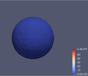
Figure 1: Left: Convergence of the algorithm with time; Right: The contour plot of the electron density of helium atom.

Example 2.

A $H_{2}$ molecule

We consider the gradient flow model for a $H_{2}$ molecule with orbits number N = 2 on $\Omega_{2}=(-20,20)^{3}$. In this example, we set external potential $V_{ext}(x)=-|x-r_{1}|^{-1}-|x-r_{2}|^{-1}$ and electron density $\rho=2(|u_{1}|^{2}+|u_{2}|^{2})$.The positions of nuclei are as follows: one hydrogen atom $r_{1}=(-0.7414,0,0)$ and another atom $r_{2}=(0.7414,0,0)$, respectively. The Hartree potential is obtained by solving the same Poisson equation in which its boundary conditions are given by multipole expansion [1]. The evaluation of exchange-correlation energy is the same as that in Example 1. Similar to the helium atom, the energy convergence curve with time and the contour plot of the electron density of $H_{2}$ molecule are given in Fig.2, which converge well and agree with our theoretical analysis.

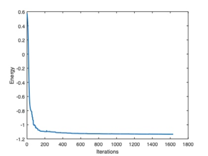
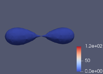
Figure 2: Left: The contour plot of the electron density of $H_{2}$ molecule; Right: Convergence of the algorithm with mesh refining.

Example 3.

A LiH molecule

We consider the gradient flow model for a lithium hydride (LiH) molecule with 2 electron orbitals. The positions of nuclei are as follows: lithium atom $R_{1}=(-1.0075,0,0)$ and hydrogen atom $R_{2}=(2.0075,0,0)$, respectively. In this example, we set external potential $V_{ext}(x)=-3\lvert x-R_{1}\rvert^{-1}-\lvert x-R_{2}\rvert^{-1}$ and electron density $\rho(x)=2(\lvert u_{1}(x)\rvert^{2}+\lvert u_{2}(x)\rvert^{2})$. The Hartree potential is obtained by solving the same Poisson equation in which its boundary conditions are given by multipole expansion [1]. The evaluation of exchange-correlation potential is the same as in Example 1. We set the computational domain $\Omega_{2}=(-10,10)^{3}$.

Fig.3 shows the results from the ground state simulation for LiH molecule. The contour of the electron density of $LiH$ molecule is shown in Fig.3 (top left), and it shows the global convergence of the total energy of LiH with the adaption refinement of the mesh as well (top right). Additionally, the mesh grids around the molecule with different number of iteration steps increasing from left to right are also shown in Fig.3 (bottom), from which we can observe that the regions with large variation of density are resolved well by mesh grids.

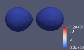
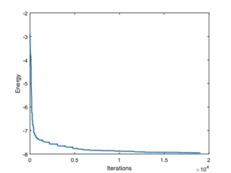
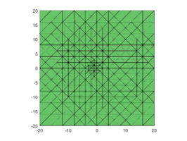
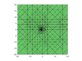
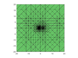
Figure 3: The results for LiH. Top left: the contour of the electron density. Top right: the global convergence history of LiH. Bottom: the mesh grids around the LiH molecule, of which the number of iteration steps increase from left to right.

6 Conclusion

This paper is devoted to show the convergence of the proposed numerical scheme for the Kohn–Sham gradient flow problem both spatially and temporally in a unified framework. Spatially, the convergence of the AFE approximation of the gradient flow model has been demonstrated by means of the boundedness of the total energy in the all-electron calculation. Temporally, motivated by [11], a linearized numerical scheme for the gradient flow model is employed in this paper, which is orthonormality preserving and has been proved to be convergent as well. Concerned with the efficiency issue, an $h$-adaptive mesh method is developed and a recovery type a posteriori error estimation technique is employed in the $h$-adaption scheme. Numerical examples successfully show the convergence of the proposed numerical scheme and confirm our theoretical results very well.

References

- [1] G. Bao, G. Hu, and D. Liu. Numerical solution of the kohn-sham equation by finite element methods with an adaptive mesh redistribution technique. Journal of Scientific Computing, 55(2):372–391, 2013.
- [2] G. Bao, G. Hu, and D. Liu. Real-time adaptive finite element solution of time-dependent Kohn–Sham equation. Journal of Computational Physics, 281:743–758, 2015.
- [3] H. Chen, X. Dai, X. Gong, L. He, and A. Zhou. Adaptive finite element approximations for Kohn–Sham models. Multiscale Modeling & Simulation, 12(4):1828–1869, 2014.
- [4] H. Chen, X. Gong, L. He, Z. Yang, and A. Zhou. Numerical analysis of finite dimensional approximations of Kohn–Sham models. Advances in Computational Mathematics, 38(2):225–256, 2013.
- [5] L. Chen. An integrated finite element method package in MATLAB. University of California at Irvine, California, 2009.
- [6] Yaoyao Chen, Yunqing Huang, and Nianyu Yi. A decoupled energy stable adaptive finite element method for cahn–hilliard–navier–stokes equations. Communications in Computational Physics, 29(4):1186–1212, 2021.
- [7] P. G. Ciarlet. The finite element method for elliptic problems. SIAM, 2002.
- [8] X. Dai, X. Gong, Z. Yang, D. Zhang, and A. Zhou. Finite volume discretizations for eigenvalue problems with applications to electronic structure calculations. Multiscale Modeling & Simulation, 9(1):208–240, 2011.
- [9] X. Dai, Z. Liu, L. Zhang, and A. Zhou. A conjugate gradient method for electronic structure calculations. SIAM Journal on Scientific Computing, 39(6):A2702–A2740, 2017.
- [10] X. Dai, Z. Liu, X. Zhang, and A. Zhou. A parallel orbital-updating based optimization method for electronic structure calculations. Journal of Computational Physics, 445:110622, 2021.
- [11] X. Dai, Q. Wang, and A. Zhou. Gradient flow based Kohn–Sham Density Functional Theory Model. Multiscale Modeling & Simulation, 18(4):1621–1663, 2020.
- [12] X. Dai, J. Xu, and A. Zhou. Convergence and optimal complexity of adaptive finite element eigenvalue computations. Numerische Mathematik, 110(3):313–355, 2008.
- [13] A. Edelman, T. A. Arias, and S. T. Smith. The geometry of algorithms with orthogonality constraints. SIAM journal on Matrix Analysis and Applications, 20(2):303–353, 1998.
- [14] C. Fiolhais, F. Nogueira, and M. A. L. Marques. A Primer in Density Functional Theory, volume 620. Springer Science & Business Media, 2003.
- [15] B. Gao, G. Hu, Y. Kuang, and X. Liu. An orthogonalization-free parallelizable framework for all-electron calculations in density functional theory. SIAM Journal on Scientific Computing, 44(3):B723–B745, 2022.
- [16] L. Genovese, B. Videau, M. Ospici, T. Deutsch, S. Goedecker, and J.-F. Méhaut. Daubechies wavelets for high performance electronic structure calculations: The bigdft project. Comptes Rendus Mécanique, 339(2-3):149–164, 2011.
- [17] Yichen Guo, Lueling Jia, Huajie Chen, Huiyuan Li, and Zhimin Zhang. A mortar spectral element method for full-potential electronic structure calculations. Communications in Computational Physics, 29(5):1541–1569, 2021.
- [18] G. Hu, T. Wang, and J. Zhou. A linearized, structure-preserving numerical scheme for the gradient flow model of Kohn–Sham density functional theory. East Asian Journal on Applied Mathematics, in press.
- [19] Y. Kuang and G. Hu. On stabilizing and accelerating SCF using ITP in solving Kohn–Sham equation. Communications in Computational Physics, 28(3):999–1018, 2020.
- [20] L. Lin, J. Lu, L. Ying, and E. Weinan. Adaptive local basis set for Kohn–Sham density functional theory in a discontinuous Galerkin framework I: Total energy calculation. Journal of Computational Physics, 231(4):2140–2154, 2012.
- [21] L. Lin and C. Yang. Elliptic preconditioner for accelerating the self-consistent field iteration in Kohn–Sham density functional theory. SIAM Journal on Scientific Computing, 35(5):S277–S298, 2013.
- [22] P. Motamarri and V. Gavini. Subquadratic-scaling subspace projection method for large-scale Kohn-Sham density functional theory calculations using spectral finite-element discretization. Physical Review B, 90(11):115127, 2014.
- [23] M. C. Payne, M. P. Teter, D. C. Allan, T. A. Arias, and J. D. Joannopoulos. Iterative minimization techniques for ab initio total-energy calculations: molecular dynamics and conjugate gradients. Reviews of modern physics, 64(4):1045, 1992.
- [24] J. P. Perdew and A. Zunger. Self-interaction correction to density-functional approximations for many-electron systems. Physical Review B, 23(10):5048, 1981.
- [25] B. G. Pfrommer, M. Côté, S. G. Louie, and M. L. Cohen. Relaxation of crystals with the quasi-newton method. Journal of Computational Physics, 131(1):233–240, 1997.
- [26] D. Russell and III. Johnson. Nist computational chemistry comparison and benchmark database. http://cccbdb.nist.gov/energy2x.asp, 2022.
- [27] Y. Shen, Y. Kuang, and G. Hu. An asymptotics-based adaptive finite element method for Kohn–Sham equation. Journal of Scientific Computing, 79(1):464–492, 2019.
- [28] N. Tancogne-Dejean, M. J. T. Oliveira, X. Andrade, H. Appel, C. H. Borca, G. Le Breton, F. Buchholz, A. Castro, S. Corni, A. A. Correa, et al. Octopus, a computational framework for exploring light-driven phenomena and quantum dynamics in extended and finite systems. The Journal of chemical physics, 152(12):124119, 2020.
- [29] T. Torsti, T. Eirola, J. Enkovaara, T. Hakala, P. Havu, V. Havu, T. Höynälänmaa, J. Ignatius, M. Lyly, I. Makkonen, et al. Three real-space discretization techniques in electronic structure calculations. physica status solidi (b), 243(5):1016–1053, 2006.
- [30] Q. Wu and T. Van Voorhis. Direct optimization method to study constrained systems within density-functional theory. Physical Review A, 72(2):024502, 2005.
- [31] J. Xu and Z. Zhang. Analysis of recovery type a posteriori error estimators for mildly structured grids. Mathematics of Computation, 73(247):1139–1152, 2004.
- [32] G. Zhang, L. Lin, W. Hu, C. Yang, and J. E. Pask. Adaptive local basis set for Kohn–Sham Density Functional Theory in a discontinuous Galerkin framework II: Force, vibration, and molecular dynamics calculations. Journal of Computational Physics, 335:426–443, 2017.
- [33] X. Zhang, J. Zhu, Z. Wen, and A. Zhou. Gradient type optimization methods for electronic structure calculations. SIAM Journal on Scientific Computing, 36(3):C265–C289, 2014.