Key observable for linear thermalization

Abstract

For studies on thermalization of an isolated quantum many-body system, the fundamental issue is to determine whether a given system thermalizes or not. However, most studies tested only a small number of observables, and it was unclear whether other observables thermalize. Here, we study whether ‘linear thermalization’ occurs for all additive observables: We consider a quantum many-body system prepared in an equilibrium state and its unitary time evolution induced by a small change $\Delta f$ of a physical parameter $f$ of the Hamiltonian, and examine whether all additive observables relax to the equilibrium values in a manner fully consistent with thermodynamics up to the linear order in $\Delta f$. We find that the additive observable conjugate to $f$ is key for linear thermalization in that its linear thermalization guarantees, under physically reasonable conditions, linear thermalization of all additive observables. Such a linear thermalization occurs in the timescale of $\mathcal{O}(|\Delta f|^{0})$, and lasts at least for a period of $o(1/\sqrt{|\Delta f|})$. We also consider linear thermalization against the change of other parameters, and find that linear thermalization of the key observable against $\Delta f$ guarantees its linear thermalization against small changes of any other parameters. Furthermore, we discuss the generalized susceptibilities for cross responses and their consistency between quantum mechanics and thermodynamics. We demonstrate our main result by performing numerical calculations for spin models. The present paper offers an efficient way of judging linear thermalization because it guarantees that examination of the single key observable is sufficient.

I Introduction

Thermalization of isolated quantum many-body systems has long been studied as the question of how the thermal equilibrium state arises from the quantum unitary dynamics [1, 2, 3, 4, 5, 6, 7, 8, 9, 10, 11, 12, 13, 14, 15, 16, 17, 18, 19, 20, 21, 22, 23, 24, 25, 26, 27, 28, 29, 30, 31, 32, 33, 34, 35, 36, 37, 38, 39, 40, 41, 42, 43, 44, 45, 46, 47, 48, 49, 50, 51, 52, 53, 54, 55, 56, 57, 58, 59, 60, 61].

As in classical systems, the relation of thermalization with chaos has been attracting much attention. It has brought a wealth of findings [7, 16, 17, 59], such as the relations to the scrambling [62, 63, 64], which was originally discussed in quantum information theory [65, 66, 67], and to the out-of-time-ordered correlations [68, 69, 70, 71, 72], which characterize the dynamical feature of quantum chaos [72, 73, 74].

Many studies have also been devoted to the eigenstate thermalization hypothesis (ETH) [1, 4, 5], which states that every energy eigenstate represents an equilibrium state. This hypothesis leads to thermalization, and is expected to hold in quantum chaotic systems [11, 12, 13, 14, 23, 16, 17]. However, since there also exist many systems that do not satisfy the ETH, how universally it holds and when it fails are still the subjects of active research [24, 25, 26, 27, 28, 29, 30, 31, 32, 33]. Furthermore, while the ETH is a sufficient condition for thermalization, whether it is also a necessary condition seems to be controversial because the answer depends on the choices of the initial state and observables that are employed to check thermalization [22, 24, 25].

Researches in the opposite directions, i.e., mechanisms for absence of thermalization and related problems in nonthermalizing systems, are also attracting much attention. They include integrable systems [75, 76, 77, 78, 79, 80, 81, 82, 83, 84, 85, 86, 87], many-body localization [88, 89, 90, 91, 92, 93, 94, 95, 96, 97, 98, 99, 100, 101, 51, 102, 103, 104, 105], many-body scars [106, 5, 46, 107, 108, 109, 110, 111, 112, 113, 114, 115, 116, 117], and Hilbert space fragmentation [118, 119, 120, 121, 122, 123, 124], which lead to absence of thermalization and failure of the ETH.

In such nonthermalizing systems, the entanglement entropy of energy eigenstate often behaves anomalously [125, 126, 108, 118, 119], and hence is sometimes employed to discriminate between thermal and nonthermal eigenstates [108, 127, 128, 129, 130]. However, even if the entanglement entropy agrees with thermodynamic entropy, it does not necessarily imply that the eigenstate represents the equilibrium state because there exist many quantum states with the same entanglement entropy. For this reason, many studies examined the expectation values of observables to discriminate between thermal and nonthermal states [42, 47, 131, 132, 133, 18, 134].

When testing thermalization using observables, most of previous studies examined only a small number of observables [42, 47, 131, 11, 132, 133, 18, 12, 13, 14, 134, 22, 16]. However, thermalization of such observables does not necessarily guarantee thermalization of other observables. For example, the authors showed in Fig. 2(b) and (c) of Ref. [135] that, in the XXZ and the XY spin chains, the magnetization of any nonzero wavenumber (such as the staggered magnetization) thermalizes while the uniform (zero wavenumber) magnetization does not. A simpler example is the case where thermalization trivially occurs by symmetry. For instance, when both the Hamiltonian and the initial state are symmetric under spin rotation by $\pi$ around the $z$ axis, the $x$ component of magnetization is kept $0$ under the unitary time evolution (because of the symmetry) and hence thermalizes trivially. Nevertheless, if this system is integrable many other observables such as interactions between nearest neighbor spins do not thermalize, as in the case of Model III of this paper. Another example, which seems nontrivial and most interesting, is the possibility that all one-body observables thermalize whereas two- and more-body observables do not. All these examples show that thermalization of some observables does not necessarily imply thermalization of all observables.

These issues have also been long-standing questions even in the linear nonequilibrium regime. For example, Kubo stated in his famous paper on the ‘Kubo formula’ [136] that if the system has an ‘ergodic property’ then his formula would give the isothermal response. However, his discussion turned out wrong [137, 138, 139]: Later studies proved that the Kubo formula gives the adiabatic response under certain conditions [137, 138, 139, 135], and it can also give the isothermal response under another condition by taking the limit of vanishing wavenumber [135]. However, the conditions given by these studies were for individual observables, which do not guarantee the conditions for all observables. In other words, the above-mentioned fundamental issue of thermalization has left unsolved even in the linear nonequilibrium regime.

In this paper, we study the unitary time evolution induced by a small change (quench) $\Delta f$ of a physical parameter $f$, and examine whether the quantum state relaxes to an equilibrium state that is fully consistent with thermodynamics up to $\mathcal{O}(\Delta f)$. We call the relaxation in this sense linear thermalization, which is obviously necessary for thermalization against an arbitrary magnitude of $\Delta f$. We place a particular emphasis on the full consistency. That is, when comparing the quantum state with a thermal equilibrium state we examine all additive observables because thermodynamics assumes that all additive observables take macroscopically definite values in an equilibrium state [140, 141, 142], although the state is specified by only a small number of variables (such as temperature). Furthermore, we consider the case where the initial state is an equilibrium state because thermodynamics basically treats transitions between equilibrium states.

We find that the additive observable $\hat{B}$ which is conjugate to $f$ is the key observable in linear thermalization. We show rigorously that, if its expectation value relaxes to the value predicted by thermodynamics, so do the expectation values of all additive observables. Even when $\hat{B}$ is a simple one-body observable, its relaxation guarantees relaxation of all other additive observables including two- and more-body ones. In addition to this theorem, we prove two propositions which state that, under reasonable conditions, the time fluctuations of the expectation values and the variances of all additive observables are sufficiently small. These results mean that linear thermalization of the single observable $\hat{B}$ guarantees linear thermalization of all additive observables. This linear thermalization occurs in timescale of $\mathcal{O}(|\Delta f|^{0})$. We prove that it lasts at least for a period of $o(1/\sqrt{|\Delta f|})$. Furthermore, we show that linear thermalization of $\hat{B}$ against the quench of $\Delta f$ implies linear thermalization of $\hat{B}$ against the quench of any other parameters. Moreover, for the generalized susceptibilities (crossed susceptibilities) our theorem gives a necessary and sufficient condition for the consistency between quantum mechanics and thermodynamics. As demonstrations of the theorem, we present numerical results for three models of spin systems.

These results dramatically reduce the costs of experiments because a single quench experiment on the key observable in a timescale of $\mathcal{O}(|\Delta f|^{0})$ gives rich information about all additive observables, a longer time scale $o(1/\sqrt{|\Delta f|})$, and the quench of other parameters.

The paper is organized as follows. Section II explains the setup. Section III defines linear thermalization by introducing three criteria. The theorem (main result) and two propositions are summarized in Sec. IV. We discuss the timescale of linear thermalization in Sec. V, and prove the third proposition about a longer timescale. Generalized susceptibilities are analyzed in Sec. VI, where two corollaries are presented. Numerical demonstrations are given in Sec. VII. We prove the theorem and propositions in Sec. VIII. In Sec. IX, we show that our results are also applicable to the case of continuous change of $f$, and explain a relation between our main result and the ETH. Section X summarizes the paper.

II Setup

We study an isolated quantum many-body system that is defined on a lattice with $N$ sites and described by a finite dimensional Hilbert space . The system obeys the unitary time evolution generated by the Hamiltonian $\hat{H}(f)$, which depends on a physical parameter $f$  such as an external magnetic field. We use units where the reduced Planck constant $\hbar$ and the Boltzmann constant $k_{\text{B}}$ are unity.

We investigate the system prepared in an equilibrium state and its time evolution induced by a change of $f$. We specifically consider a quench process, in which $f$ is changed discontinuously. This does not mean any loss of generality because the same results can also be obtained for continuous change of $f$, as shown in Sec. IX.2.

Since we are interested in the consistency with thermodynamics, we consider the case where each equilibrium state of the system is uniquely specified macroscopically by an appropriate set of variables. Here, the number of the variables in the set is finite and independent of $N$. (This is one of the basic assumptions of thermodynamics .) To be specific, we here assume that $f$, $N$, and the inverse temperature $\beta$ is such a set of variables. Then, equilibrium states can be represented by the canonical Gibbs state

$$\hat{\rho}^{\text{can}}(\beta,f):=e^{-\beta\hat{H}(f)}/Z(\beta,f),$$ (1)

where $Z(\beta,f)$ is the partition function.

For time $t<0$, $f$ takes a constant value $f_{0}$, which defines the initial Hamiltonian,

$$\hat{H}_{0}:=\hat{H}(f_{0}),$$ (2)

and the system is in an equilibrium state at a finite inverse temperature $\beta_{0}$, represented by

$$\hat{\rho}^{\text{eq}}_{0}:=\hat{\rho}^{\text{can}}(\beta_{0},f_{0}).$$ (3)

At $t=0$, $f$ is changed from $f_{0}$ to another constant value $f_{0}+\Delta f$ discontinuously, as shown in Fig. 1(a). Due to this quench of $f$, the state for $t>0$ evolves according to the Schrödinger equation described by the postquench Hamiltonian

$$\hat{H}_{\Delta f}:=\hat{H}(f_{0}+\Delta f).$$ (4)

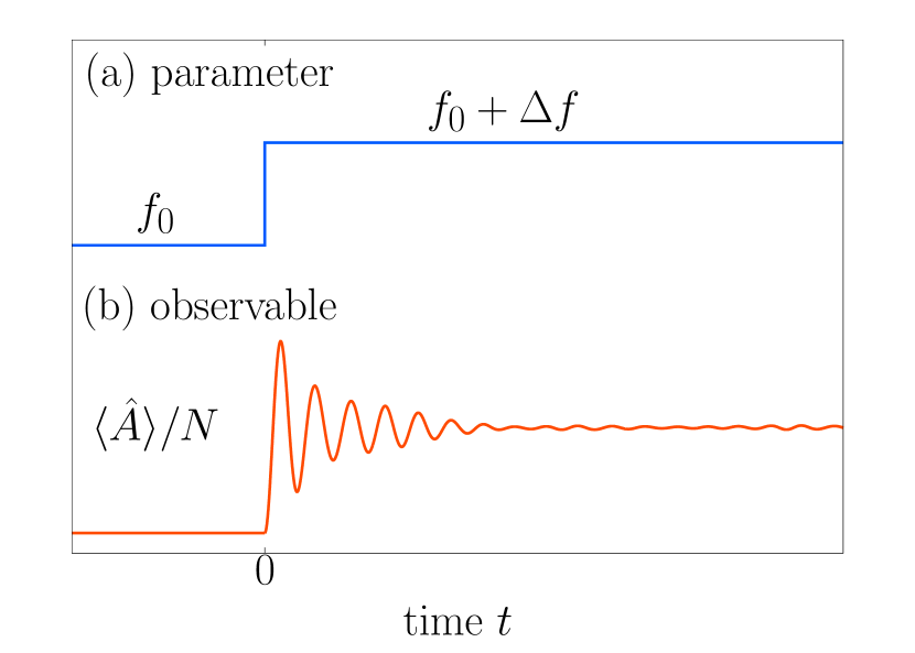
Figure 1: (a) The quench process considered in this paper. See Sec. II for details. (b) A schematic plot of typical time evolution of the expectation value of an additive observable per site after the quench at $t=0$.

Consequently the expectation values of additive observables evolve in time, as shown in Fig. 1(b). Here, we say an observable $\hat{A}$ is additive when it is the sum of local observables $\hat{a}_{{\bf\it r}}$ over the whole system,

$$\hat{A}=\sum_{{\bf\it r}}\hat{a}_{{\bf\it r}},$$ (5)

where we say an observable $\hat{a}_{{\bf\it r}}$ is local when its support consists of sites within a distance of at most $\mathcal{O}(N^{0})$ from the site ${\bf\it r}$.

Note that a local observable $\hat{a}_{{\bf\it r}}$ is not necessarily a one-body observable. It can be, say, a two-spin observable such as the one given by Eq. (41) below. Note also that the additive observable $\hat{A}$ can be noninvariant under a spatial translation. For example, for a magnetic field of a wavenumber ${\bf\it k}$ with magnitude $f$,

$$h({{\bf\it r}})=f\sin({{\bf\it k}}\cdot{{\bf\it r}}),$$ (6)

its interaction with spins,

$$-\sum_{{\bf\it r}}h({{\bf\it r}})\hat{\sigma}^{z}_{{\bf\it r}}=-f\sum_{{\bf\it r}}\sin({{\bf\it k}}\cdot{{\bf\it r}})\hat{\sigma}^{z}_{{\bf\it r}},$$ (7)

is an additive observable with $\hat{a}_{{\bf\it r}}=-h({{\bf\it r}})\hat{\sigma}^{z}_{{\bf\it r}}$. This example also shows that our theory is applicable to the case where a spatially-varying external field is applied. Since we allow such an ${\bf\it r}$-dependent coefficient in $\hat{a}_{{\bf\it r}}$, we exclude strange cases where the operator norm $\|\hat{a}_{{\bf\it r}}\|_{\infty}$ diverges as $|{\bf\it r}|\to\infty$ by imposing

$$\|\hat{a}_{{\bf\it r}}\|_{\infty}\leq C_{A}\quad\text{for all }{\bf\it r},$$ (8)

where $C_{A}$ is a constant independent of $N$ and ${\bf\it r}$. From this restriction, any additive observable $\hat{A}$ satisfies

$$\|\hat{A}\|_{\infty}=\mathcal{O}(N).$$ (9)

We also make a natural assumption that $\hat{H}(f)$ and its derivative,

$$\hat{B}:=-\frac{\partial\hat{H}}{\partial f}(f_{0}),$$ (10)

are additive observables. Indeed this assumption is satisfied for the above example of $\hat{H}(f)$ [see also Eq. (32) below]. We say that the observable $\hat{B}$ is conjugate to the parameter $f$, and vice versa.

We examine whether the system relaxes to the equilibrium state for small $|\Delta f|$. For this purpose, we consider the case where an equilibrium state exists not only for $f=f_{0}$ but also for $f=f_{0}+\Delta f$. That is, we exclude, for instance, electric conductors in a uniform electric field. Furthermore, to exclude uninteresting divergences, we also limit ourselves to the case where no phase transition occurs in the neighborhood of the initial equilibrium state. This implies that the initial equilibrium state is stable against the changes of parameters conjugate to any additive observables. (This condition is precisely expressed by Eq. (53) in Sec. VIII.1.)

III Criteria for linear thermalization

Since we consider the case of small $|\Delta f|$, we examine the consistency with thermodynamics up to the linear order in $\Delta f$: We say linear thermalization occurs for an additive observable $\hat{A}$ if the following three criteria are satisfied up to $\mathcal{O}(\Delta f)$.

Criterion (i) (consistency of expectation value): The long time average of the expectation value of $\hat{A}$ after the quench is sufficiently close to the equilibrium value. More precisely,

$$\overline{\langle\hat{A}^{\Delta f}(t)\rangle^{\text{eq}}_{0}}^{\mathcal{T}}-\langle\hat{A}\rangle^{\text{eq}}_{\Delta f}=o(N)$$ (11)

for sufficiently long time $\mathcal{T}$. (See Sec. V for detailed discussions on $\mathcal{T}$.) Here

$$\hat{A}^{\Delta f}(t):=e^{i\hat{H}_{\Delta f}t}\hat{A}e^{-i\hat{H}_{\Delta f}t}$$ (12)

is the Heisenberg operator of $\hat{A}$ evolved by $\hat{H}_{\Delta f}$, and, for any $t$-dependent quantity $g(t)$,

$$\overline{g(t)}^{\mathcal{T}}:=\frac{1}{\mathcal{T}}\int_{0}^{\mathcal{T}}\differential{t}g(t).$$ (13)

Furthermore, $\langle\bullet\rangle^{\text{eq}}_{0}:=\Tr[\hat{\rho}^{\text{eq}}_{0}\bullet\bigr{]}$ is the expectation value in the initial state $\hat{\rho}^{\text{eq}}_{0}$, while $\langle\bullet\rangle^{\text{eq}}_{\Delta f}:=\Tr[\hat{\rho}^{\text{eq}}_{\Delta f}\bullet\bigr{]}$ is the expectation value in

$$\hat{\rho}^{\text{eq}}_{\Delta f}:=\hat{\rho}^{\text{can}}(\beta_{\Delta f},f_{0}+\Delta f).$$ (14)

The latter state $\hat{\rho}^{\text{eq}}_{\Delta f}$ represents the final equilibrium state predicted by thermodynamics. Its inverse temperature $\beta_{\Delta f}$ is determined from energy conservation

$$\langle\hat{H}_{\Delta f}\rangle_{\Delta f}^{\text{eq}}=\langle\hat{H}_{\Delta f}\rangle_{0}^{\text{eq}}.$$ (15)

Note that $\beta_{\Delta f}\neq\beta_{0}$ even in $\mathcal{O}(\Delta f)$, as explicitly given by Eq. (82) in Appendix A.1.

Criterion (ii) (equilibration): At almost all $t>0$, the expectation value of $\hat{A}$ is sufficiently close to its long time average. That is, their difference is macroscopically negligible in the sense that

$$\overline{\Bigl{|}\langle\hat{A}^{\Delta f}(t)\rangle^{\text{eq}}_{0}-\overline{\langle\hat{A}^{\Delta f}(t)\rangle^{\text{eq}}_{0}}^{\mathcal{T}}\Bigr{|}^{2}}^{\mathcal{T}}=o(N^{2})$$ (16)

for sufficiently long time $\mathcal{T}$.

Criterion (iii) (smallness of variance): At almost all $t>0$, the variance of $\hat{A}$ is macroscopically negligible such that

$$\overline{\text{Var}_{0}[\hat{A}^{\Delta f}(t)]}^{\mathcal{T}}=o(N^{2})$$ (17)

for sufficiently long time $\mathcal{T}$. Here $\text{Var}_{0}[\hat{\bullet}]:=\langle(\hat{\bullet})^{2}\rangle^{\text{eq}}_{0}-(\langle\hat{\bullet}\rangle^{\text{eq}}_{0})^{2}$.

Thermodynamics assumes that all additive observables take macroscopically definite values in an equilibrium state [140, 141, 142]. Since we are interested in full consistency with thermodynamics, we examine whether linear thermalization occurs, i.e., whether these criteria are satisfied, for all additive observables.

IV Summary of results

Among three criteria of the previous section, Criterion (i) has been studied most intensively because in many cases it discriminates thermalizing systems from nonthermalizing ones. For instance, it was observed in many integrable systems that relaxation to some steady states occurs, indicating that Criteria (ii) and (iii) are satisfied, whereas they are nonthermal states, which do not satisfy Criterion (i) [75, 78, 76, 77, 41, 43, 44].

Therefore we place a theorem about Criterion (i) as our main result. We also obtain additional results which show that Criteria (ii) and (iii) are easily satisfied in our setting, under conditions weaker than those of previous studies [146, 147, 7]. These results are summarized in this section. We will extend them slightly in Sec. V, and thereby discuss the timescale of the linear thermalization.

IV.1 Theorem for Criterion (i)

Our main result is that if the additive observable $\hat{B}$ conjugate to $f$, given by Eq. (10), satisfies Criterion (i) of Sec. II up to $\mathcal{O}(\Delta f)$, then so do all additive observables. To be precise, we obtain
Theorem (main result):

$$\lim_{\mathcal{T}\to\infty}\lim_{\Delta f\to 0}\frac{\overline{\langle\hat{A}^{\Delta f}(t)\rangle^{\text{eq}}_{0}}^{\mathcal{T}}-\langle\hat{A}\rangle^{\text{eq}}_{\Delta f}}{\Delta f}=o(N)$$ (18)

holds for every additive observable $\hat{A}$ if and only if it holds for $\hat{A}=\hat{B}$,

$$\lim_{\mathcal{T}\to\infty}\lim_{\Delta f\to 0}\frac{\overline{\langle\hat{B}^{\Delta f}(t)\rangle^{\text{eq}}_{0}}^{\mathcal{T}}-\langle\hat{B}\rangle^{\text{eq}}_{\Delta f}}{\Delta f}=o(N).$$ (19)

This theorem identifies $\hat{B}$, which is conjugate to $f$, as the key observable for linear thermalization of all additive observables. That is, one can judge whether the long time average of the expectation value of every additive observable $\hat{A}$ is consistent with thermodynamics by examining the single observable $\hat{B}$. This striking result has the following significant features.

Firstly, it is in sharp contrast with the existing approaches to Criterion (i) [11, 12, 13, 14, 148, 15], such as the ETH. In fact, previous studies clarified that the ETH for an observable implies Criterion (i) for that observable. However, it did not guarantee either the ETH or Criterion (i) for other observables. By contrast, our Theorem does guarantee that Criterion (i) is satisfied by all additive observables up to $\mathcal{O}(\Delta f)$ if it is satisfied by $\hat{B}$. (We will demonstrate this point numerically in Sec. VII.) This result may be most surprising in the case where $\hat{B}$ is a one-body observable: If Eq. (19) holds for that one-body observable, then it also holds for all other additive observables including two- and more-body ($\mathcal{O}(N^{0})$-body) ones.

Secondly, the ETH for $\hat{B}$ implies condition (19) but the converse is not necessarily true, as will be discussed in Sec. IX.3.

Thirdly, our Theorem has significant meanings about the generalized susceptibilities for cross responses, as will be discussed in Sec. VI.

Fourthly, we can extend the result such that $\hat{A}$ and $\hat{B}$ in Eqs. (18) and (19) are not restricted to additive observables, as will be discussed in Sec. IX.1.

IV.2 Proposition for Criterion (ii)

Under the reasonable condition that $\hat{H}_{0}$ does not have exponentially many resonances, all additive observables satisfy Criterion (ii) up to $\mathcal{O}(\Delta f)$. That is, we obtain
Proposition $1$: If the maximum number of resonances $D_{\text{res}}$ [defined by Eq. (54) in Sec. VIII.2] satisfies

$$D_{\text{res}}\Tr[(\hat{\rho}^{\text{eq}}_{0})^{2}\bigr{]}=o(1/N^{2}),$$ (20)

then

$$\lim_{\mathcal{T}\to\infty}\lim_{\Delta f\to 0}\overline{\biggl{|}\frac{\langle\hat{A}^{\Delta f}(t)\rangle^{\text{eq}}_{0}-\overline{\langle\hat{A}^{\Delta f}(t)\rangle^{\text{eq}}_{0}}^{\mathcal{T}}}{\Delta f}\biggr{|}^{2}}^{\mathcal{T}}=o(N^{2})$$ (21)

for every additive observable $\hat{A}$. [A detailed expression of the right-hand side (r.h.s) will be given in Sec. VIII.2.]

This proposition is obtained by adapting the argument of Short and Farrelly [146] to our setting. While their result contains the effective dimension of the initial state, our condition (20) instead contains its purity $\Tr[(\hat{\rho}^{\text{eq}}_{0})^{2}\bigr{]}$. Since the postquench Hamiltonian $\hat{H}_{\Delta f}$ is different from the initial Hamiltonian $\hat{H}_{0}$, evaluation of the effective dimension of the initial state $\hat{\rho}^{\text{eq}}_{0}$ in terms of $\hat{H}_{\Delta f}$ is not an easy task. By contrast, its purity can be evaluated easily as shown in Appendix A.2.

Note that our condition is weaker than the “nonresonance condition,” $D_{\text{res}}=1$, of the previous studies [6, 149, 150]. The nonresonance condition often fails even in nonintegrable systems, e.g., when energy eigenvalues have degeneracies due to symmetries. By contrast, condition (20) is expected to hold not only in such systems but also in wider classes of systems, including interacting integrable systems (such as Model III of Sec. VII), because

$$\Tr[(\hat{\rho}^{\text{eq}}_{0})^{2}\bigr{]}=e^{-\Theta(N)}$$ (22)

at any nonzero temperature $1/\beta_{0}$ as shown in Appendix A.2.

IV.3 Proposition for Criterion (iii)

Under the reasonable condition that the fluctuation of every additive observable in the initial equilibrium state is sufficiently small, the variances of all additive observables after the quench remain small enough such that Criterion (iii) is satisfied up to $\mathcal{O}(\Delta f)$. To be precise, we find
Proposition $2$: If the fourth order central moment of every additive observable $\hat{A}$ in the initial state satisfies

$$\langle(\hat{A}-\langle\hat{A}\rangle^{\text{eq}}_{0})^{4}\rangle^{\text{eq}}_{0}=\mathcal{O}(N^{2}),$$ (23)

then

$$\lim_{\mathcal{T}\to\infty}\lim_{\Delta f\to 0}\left|\frac{\overline{\text{Var}_{0}[\hat{A}^{\Delta f}(t)]}^{\mathcal{T}}-\text{Var}_{0}[\hat{A}]}{\Delta f}\right|=\mathcal{O}\bigl{(}N^{\frac{3}{2}}\bigr{)}$$ (24)

for every additive observable $\hat{A}$. [A detailed expression of the r.h.s will be given as Eq. (62) in Sec. VIII.3.]

Note that condition (23) also bounds the variance in the initial state as

$$\text{Var}_{0}[\hat{A}]\leq\sqrt{\langle(\hat{A}-\langle\hat{A}\rangle^{\text{eq}}_{0})^{4}\rangle^{\text{eq}}_{0}}=\mathcal{O}(N),$$ (25)

which follows from the Cauchy-Schwarz inequality. By inserting this into Eq. (24), we have 

$$\overline{\text{Var}_{0}[\hat{A}^{\Delta f}(t)]}^{\mathcal{T}}=\mathcal{O}(N)+\Delta f\times\mathcal{O}\bigl{(}N^{\frac{3}{2}}\bigr{)}+o(\Delta f),$$ (26)

which shows that Criterion (iii) is satisfied up to $\mathcal{O}(\Delta f)$.

Since we exclude phase transition points, our condition (23) seems plausible. By contrast, previous results on Criterion (iii) [147, 59] required a condition that is stronger than the ETH. The above proposition shows that the criterion is satisfied under a much weaker condition in our setting.

To sum up these theorem and propositions, linear thermalization of the single key observable $\hat{B}$ guarantees linear thermalization of all additive observables, under physically reasonable conditions.

V Timescale of linear thermalization

When studying thermalization theoretically, it is customary to take the limit $\mathcal{T}\to\infty$ [59, 61], as we did above. However, more detailed information about the timescale is necessary because in experiments thermalization occurs in reasonably short timescales [42, 47]. The timescale is particularly nontrivial when “prethermalization” [152, 153, 154, 155, 156, 61, 157] occurs, i.e., when the system first relaxes to a nonthermal quasi-steady state, and at some time stage after that, it relaxes to a true thermal equilibrium state. In nearly integrable systems, the timescale for the relaxation to a true thermal equilibrium state crucially depends on the magnitude of $\Delta f$ and is typically of $\Theta(1/|\Delta f|^{2})$ [158, 159, 160, 161]. Thus the $\Delta f$ dependence of the timescale is very important. In this section, we investigate it for linear thermalization.

V.1 Timescale of linear thermalization in Theorem and Propositions $1$ and $2$

Our results of Sec. IV, namely Theorem and Propositions $1$ and $2$, take the two limits $\mathcal{T}\to\infty$ and $\Delta f\to 0$ in the following order :

$$\lim_{\mathcal{T}\to\infty}\lim_{\Delta f\to 0}[\mbox{function of $\mathcal{T}$ and $\Delta f$]}.$$ (27)

In this order of limits, $\mathcal{T}$ is smaller than any timescale that grows as $\Delta f\to 0$ . That is, it extracts the behavior of the system in the time interval $[0,\mathcal{T}]$ such that $\mathcal{T}=\Theta(|\Delta f|^{0})$. This leads to the following observations:
Timescale in Theorem and Propositions $1$ and $2$: ($1$) If linear thermalization occurs in the limit (27), as in Theorem and Propositions $1$ and $2$, then it occurs in some $t=\mathcal{O}(|\Delta f|^{0})$, as illustrated in Fig. 2(a). ($2$) On the other hand, if linear thermalization does not occur in the limit (27), then it does not occur in any timescale of $\mathcal{O}(|\Delta f|^{0})$, as in Fig. 2(b).

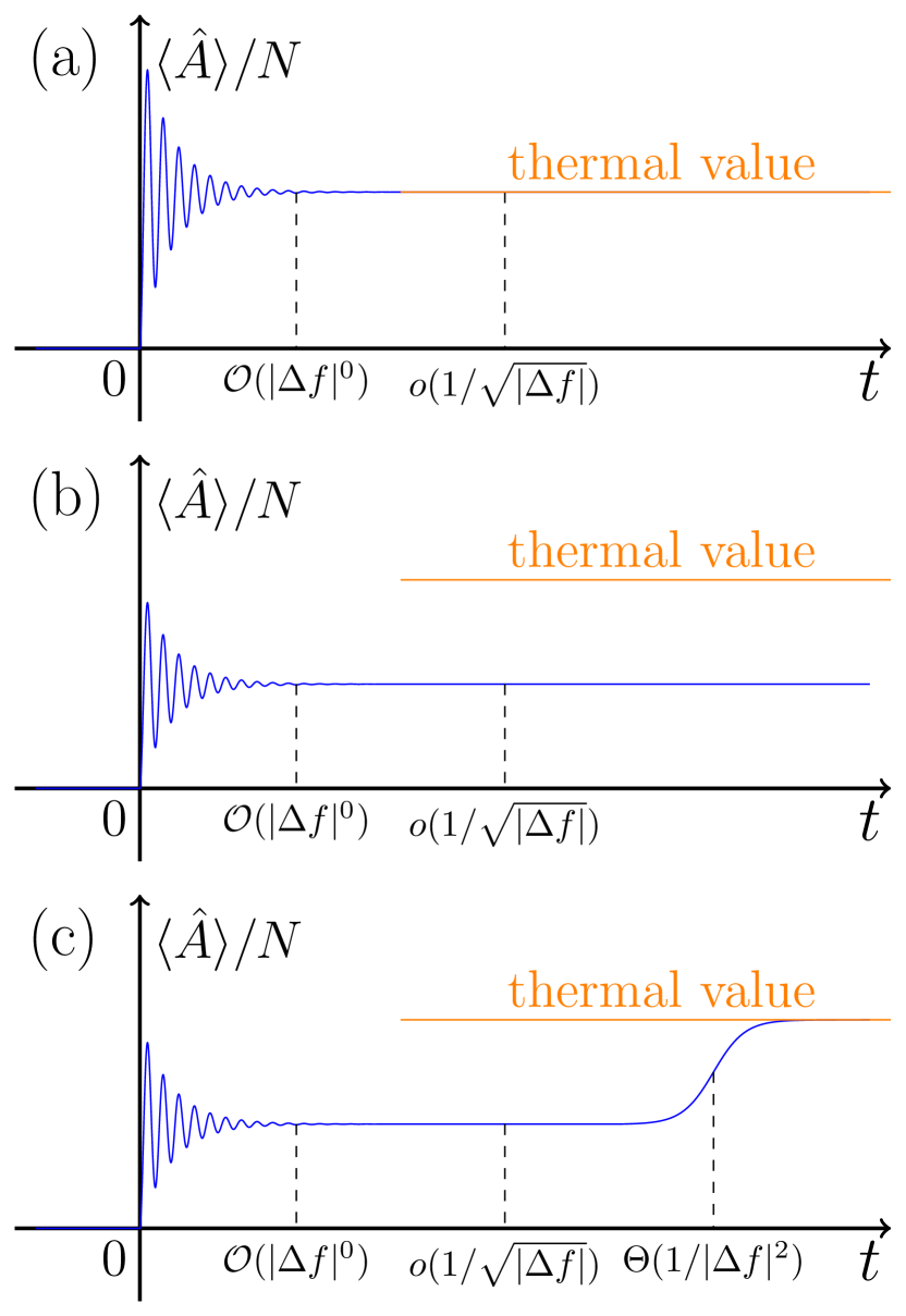
Figure 2: Schematic plots of the time evolution of $\langle\hat{A}^{\Delta f}(t)\rangle^{\text{eq}}_{0}/N$ in three typical cases. (a) Linear thermalization occurs, corresponding to cases ($1$) of Sec. V.1 and ($1^{\prime}$) of V.2. (b) Linear thermalization does not occur, corresponding to cases ($2$) of Sec. V.1 and ($2^{\prime}$) of V.2. (c) Prethermalization occurs, which is discussed in Sec. V.3.

That is, the timescale of thermalization is independent of the magnitude of $\Delta f$. Behaviors in longer timescales will be discussed in the following two subsections.

V.2 Extension to a longer timescale

We now extend our results to a longer timescale $o(1/\sqrt{|\Delta f|})$, and explain its implications for linear thermalization.

Let $\mathcal{T}_{\Delta f}$ be a timescale that grows as $\Delta f\to 0$ satisfying $\mathcal{T}_{\Delta f}=o(1/\sqrt{|\Delta f|})$. As will be shown in Sec. VIII.4, we find that the values of the left-hand sides of Eqs. (18), (21) and (24) do not change when the limit (27) is replaced with

$$\lim_{\Delta f\to 0}[\mbox{function of $\mathcal{T}$ and $\Delta f$ with $\mathcal{T}$ replaced by $\mathcal{T}_{\Delta f}$]}.$$ (28)

That is, we obtain the following proposition .
Proposition 3: For any $\mathcal{T}_{\Delta f}=o(1/\sqrt{|\Delta f|})$ and for any additive observable $\hat{A}$,

$$\lim_{\Delta f\to 0}\frac{\overline{\langle\hat{A}^{\Delta f}(t)\rangle^{\text{eq}}_{0}}^{\mathcal{T}_{\Delta f}}-\langle\hat{A}\rangle^{\text{eq}}_{\Delta f}}{\Delta f}$$

$$=\lim_{\mathcal{T}\to\infty}\lim_{\Delta f\to 0}\frac{\overline{\langle\hat{A}^{\Delta f}(t)\rangle^{\text{eq}}_{0}}^{\mathcal{T}}-\langle\hat{A}\rangle^{\text{eq}}_{\Delta f}}{\Delta f},$$ (29)

$$\lim_{\Delta f\to 0}\overline{\biggl{|}\frac{\langle\hat{A}^{\Delta f}(t)\rangle^{\text{eq}}_{0}-\overline{\langle\hat{A}^{\Delta f}(t)\rangle^{\text{eq}}_{0}}^{\mathcal{T}_{\Delta f}}}{\Delta f}\biggr{|}^{2}}^{\mathcal{T}_{\Delta f}}$$

$$=\lim_{\mathcal{T}\to\infty}\lim_{\Delta f\to 0}\overline{\biggl{|}\frac{\langle\hat{A}^{\Delta f}(t)\rangle^{\text{eq}}_{0}-\overline{\langle\hat{A}^{\Delta f}(t)\rangle^{\text{eq}}_{0}}^{\mathcal{T}}}{\Delta f}\biggr{|}^{2}}^{\mathcal{T}},$$ (30)

$$\lim_{\Delta f\to 0}\frac{\overline{\text{Var}_{0}[\hat{A}^{\Delta f}(t)]}^{\mathcal{T}_{\Delta f}}-\text{Var}_{0}[\hat{A}]}{\Delta f}$$

$$=\lim_{\mathcal{T}\to\infty}\lim_{\Delta f\to 0}\frac{\overline{\text{Var}_{0}[\hat{A}^{\Delta f}(t)]}^{\mathcal{T}}-\text{Var}_{0}[\hat{A}]}{\Delta f}.$$ (31)

This proposition shows that Theorem, Propositions 1 and 2 hold even when $\mathcal{T}$ is replaced with a longer timescale $\mathcal{T}_{\Delta f}$, and leads to the following observations:
Timescale of linear thermalization: ($1^{\prime}$) If linear thermalization occurs in some $t=\mathcal{O}(|\Delta f|^{0})$, it lasts at least for a period of $o(1/\sqrt{|\Delta f|})$. Conversely, if linear thermalization occurs at some $o(1/\sqrt{|\Delta f|})$, it already occurs at some $t=\mathcal{O}(|\Delta f|^{0})$. See Fig. 2(a). ($2^{\prime}$) On the other hand, absence of linear thermalization in a shorter timescale of $\mathcal{O}(|\Delta f|^{0})$ guarantees its absence in a longer timescale of $o(1/\sqrt{|\Delta f|})$, and vice versa. See Fig. 2(b).

This result, together with the results of Secs. IV and V.1, implies, in particular, that linear thermalization of the single key observable $\hat{B}$ in the timescale of $\mathcal{O}(|\Delta f|^{0})$ guarantees linear thermalization of all additive observables not only in the same timescale but also in a longer timescale of $o(1/\sqrt{|\Delta f|})$.

V.3 Stationarity and implications for prethermalization

We here discuss stationarity of the system and its implication for prethermalization.

From Eqs. (29)–(31), we obtain the following observations:
Stationarity throughout a certain time region: Suppose that conditions (20) and (23) for Propositions 1 and 2 are fulfilled. Then, throughout a time region from $\mathcal{O}(|\Delta f|^{0})$ to $o(1/\sqrt{|\Delta f|})$, all additive observables take macroscopically definite and stationary values, up to $\mathcal{O}(\Delta f)$. In other words, the system relaxes to a macroscopic state and stays in the same macroscopic state throughout this time region, up to $\mathcal{O}(\Delta f)$.

Note that this stationary state can be either thermal or nonthermal, depending on whether condition (19) of our Theorem is satisfied or not. If the state is thermal as illustrated in Fig. 2(a), it means that linear thermalization occurs. On the other hand, if the state is nonthermal [i.e., if condition (19) is not satisfied] as in Fig. 2(b), it is a nonthermal stationary state.

The latter case includes systems which exhibit prethermalization [152, 153, 154, 155, 156, 61, 157]. The prethermalization often occurs when $\Delta f$ switches the system from integrable to nonintegrable. (Shiraishi proved the existence of a system in which such switching is possible by an arbitrary nonvanishing value of $\Delta f$ [165].) In a typical case of such prethermalization, the system first relaxes to a nonthermal stationary state in some timescale of $\mathcal{O}(|\Delta f|^{0})$, and then relaxes to the true thermal equilibrium state at some timescale of $\Theta(1/|\Delta f|^{2})$ [61], as illustrated in Fig. 2(c). For such a system, our results detect the nonthermal stationary state in the time region from $\mathcal{O}(|\Delta f|^{0})$ to $o(1/\sqrt{|\Delta f|})$ and the absence of linear thermalization in this time region.

VI Generalized Susceptibilities for Cross Responses

Our Theorem has significant meanings about the generalized susceptibilities for cross responses.

In response to the change of a parameter (such as an external field), not only its conjugate observable $\hat{B}$ but also other observables often change their values. The magnetoelectric effect and the piezoelectric effect are well-known examples. Such responses of observables $\hat{A}$ that are not conjugate to the changed parameter are called cross responses, and have been attracting much attention [166, 167, 168, 169, 170]. They are characterized by the generalized susceptibilities (crossed susceptibilities), which we denote by $\chi(A|B)$.

For example, when a magnetic field of an arbitrary wavenumber ${\bf\it k}$, Eq. (6), is applied to a spin system, Eq. (7) yields the additive observable conjugate to $f$ as

$$\hat{B}=\sum_{{\bf\it r}}\sin({{\bf\it k}}\cdot{{\bf\it r}})\hat{\sigma}^{z}_{{\bf\it r}},$$ (32)

which is the total magnetization $\hat{M}_{{\bf\it k}}$ of wavenumber ${\bf\it k}$. Then, if we take $\hat{A}$ to be the total electric polarization $\hat{P}_{{\bf\it k}}$ of wavenumber ${\bf\it k}$ the generalized susceptibility $\chi(A|B)$ is the magnetoelectric susceptibility at wavenumber ${\bf\it k}$ , whereas if we take $\hat{A}=\hat{B}=\hat{M}_{{\bf\it k}}$ the corresponding susceptibility $\chi(B|B)$ is just the ordinary magnetic susceptibility at wavenumber ${\bf\it k}$.

We here compare two types of generalized susceptibilities. One is $\chi(A|B)$ obtained in quantum mechanics,

$$\chi^{\text{QM}}_{N}(A|B) :=\lim_{\mathcal{T}\to\infty}\lim_{\Delta f\to 0}\frac{\overline{\langle\hat{A}^{\Delta f}(t)\rangle^{\text{eq}}_{0}}^{\mathcal{T}}-\langle\hat{A}\rangle^{\text{eq}}_{0}}{\Delta fN},$$ (33)

which is defined by the Schrödinger dynamics. The other is $\chi(A|B)$ predicted by thermodynamics ,

$$\chi^{\text{TD}}_{N}(A|B) :=\lim_{\Delta f\to 0}\frac{\langle\hat{A}\rangle^{\text{eq}}_{\Delta f}-\langle\hat{A}\rangle^{\text{eq}}_{0}}{\Delta fN},$$ (34)

where the final state $\hat{\rho}^{\text{eq}}_{\Delta f}$ is determined by thermodynamics and equilibrium statistical mechanics using the energy conservation, Eq. (15).

From these definitions, Eqs. (18) and (19) are equivalent to

$$\lim_{N\to\infty}\chi^{\text{QM}}_{N}(A|B) =\lim_{N\to\infty}\chi^{\text{TD}}_{N}(A|B),$$ (35)

$$\lim_{N\to\infty}\chi^{\text{QM}}_{N}(B|B) =\lim_{N\to\infty}\chi^{\text{TD}}_{N}(B|B),$$ (36)

respectively. Therefore, our Theorem can be rephrased as follows.
Consistency of cross responses: Equation (35) holds for every additive observable $\hat{A}$ if it holds for $\hat{B}$.

Furthermore, the following symmetries follow from Eqs. (81) and (84) in Appendix A.2:

$$\chi^{\text{QM}}_{N}(A|B) =\chi^{\text{QM}}_{N}(B|A),$$ (37)

$$\chi^{\text{TD}}_{N}(A|B) =\chi^{\text{TD}}_{N}(B|A).$$ (38)

(The latter is just a Maxwell relation of thermodynamics.) From these relations, Eq. (35) can be rewritten as

$$\lim_{N\to\infty}\chi^{\text{QM}}_{N}(B|A) =\lim_{N\to\infty}\chi^{\text{TD}}_{N}(B|A).$$ (39)

Therefore, we obtain the following result.
Corollary 1 (consistency of responses to other parameters): Equation (39) holds for every additive observable $\hat{A}$ if Eq. (36) holds for $\hat{B}$.

That is, the quantum-mechanical response of an additive observable $\hat{B}$ to the parameter $f_{A}$ conjugate to an arbitrary additive observable $\hat{A}$ is consistent with thermodynamics if the quantum-mechanical response of $\hat{B}$ to its own conjugate parameter $f$ is consistent with thermodynamics.

Moreover, this corollary has the following implication for linear thermalization.
Corollary 2: Under the conditions (20) and (23) for Propositions 1 and 2, linear thermalization of $\hat{B}$ against the quench of its conjugate parameter $f$ implies linear thermalization of the same observable $\hat{B}$ against the quench of any other parameter $f_{A}$ that is conjugate to an arbitrary additive observable $\hat{A}$.

These corollaries dramatically reduce the costs of experiments and theoretical calculations of linear thermalization and cross responses. For example, suppose that one wants to examine the cross response of the magnetization $\hat{M}$ of a spin system against the quench of an interaction parameter $J$, whose quench is, however, technically difficult. In such a case, one can perform an alternative experiment in which an external magnetic field that is conjugate to $\hat{M}$ is quenched. If the quantum-mechanical response of $\hat{M}$ is consistent with thermodynamical one in the latter experiment, then Corollary $1$ guarantees their consistency in the former experiment.

VII Examples

In this section, we demonstrate our Theorem using one-dimensional spin systems. For a nonintegrable model, we first show linear thermalization of $\hat{B}$, which implies, according to our Theorem, linear thermalization of all other $\hat{A}$’s. We demonstrate it for typical $\hat{A}$’s. We also present integrable models in which linear thermalization does not occur neither for $\hat{B}$ nor for typical $\hat{A}$’s.

VII.1 Models

If a system had many symmetries, one would have to investigate thermalization separately in individual symmetry sectors not to overlook the degeneracy of energy eigenvalues. To avoid such complicated procedures, we construct our model Hamiltonian by adding two extra terms to the one-dimensional XYZ model in a magnetic field [165] as

$$\hat{H} =-\sum_{r=1}^{N}\Bigl{(}J_{xx}\hat{\sigma}_{r}^{x}\hat{\sigma}_{r+1}^{x}+J_{yy}\hat{\sigma}_{r}^{y}\hat{\sigma}_{r+1}^{y}+J_{zz}\hat{\sigma}_{r}^{z}\hat{\sigma}_{r+1}^{z}+h_{z}\hat{\sigma}^{z}_{r}$$

$$\hskip 48.0pt+J_{yz}\hat{\sigma}_{r}^{y}\hat{\sigma}_{r+1}^{z}+h_{x}\hat{\sigma}_{r}^{x}\Bigr{)},$$ (40)

where $\hat{\sigma}_{N+1}^{\mu}=\hat{\sigma}_{1}^{\mu}$ ($\mu=x,y,z$). The last two terms are the extra terms that break all known symmetries, except for the translation symmetry, of the conventional XYZ model in a magnetic field. Indeed, the $J_{yz}$ term breaks the lattice inversion symmetry and the spin $\pi$ rotation symmetry around $z$ axis. Furthermore, the $J_{yz}$ and the $h_{x}$ terms break the complex conjugate symmetry.

We believe this model, when all parameters are nonzero and $J_{xx}\neq J_{yy}$, is nonintegrable in the sense that it has no local conserved quantities other than the Hamiltonian, because so is the conventional model with $J_{yz}=h_{x}=0$ [165]. As a support of this belief, we have confirmed in Appendix B.3 that the energy level statistics in each momentum sector is described by the Gaussian unitary ensemble (GUE) of the random matrix theory [173, 88, 174].

We tabulate the values of the parameters used in the numerical calculations as Model I in Table 1. The values are taken in such a way that the ratio of every two of them is irrational in order to avoid a possible accidental symmetry.

Table 1: Values of the parameters in the Hamiltonian, Eq. (40), for the three models.

Model	$J_{xx}$	$J_{yy}$	$J_{zz}\ (=f)$	$h_{z}$	$J_{yz}$	$h_{x}$
	fixed	fixed	initial value $f_{0}$	fixed	fixed	fixed
I (nonintegrable)	$\cos 1$	$1$	$e$	$\ln 5$	$\ln 3$	$\pi$
II (integrable)	$0$	$1$	$e$	$0$	$\ln 3$	$\pi$
III (integrable)	$1$	$1$	$e$	$\ln 5$	$0$	$0$

For comparison, we also study Model II in which $J_{xx}=h_{z}=0$ (see Table 1). Although this model is slightly different from known models [175], we find it integrable in the sense that it can be mapped to a noninteracting fermionic system by the Jordan-Wigner transformation. We give its analytic solutions in Appendix C.

In addition, Model III in which $J_{xx}=J_{yy}$ and $J_{yz}=h_{x}=0$ (see Table 1) is studied. It is just the XXZ model, whose energy eigenstates and additive conserved quantities are constructed by using the Bethe ansatz [176, 177, 178, 179, 180, 181, 182, 183, 184].

These models cover three typical types of systems: the nonintegrable systems, the “noninteracting integrable systems,” and the “interacting integrable systems” that are solvable by the Bethe ansatz.

In all these models, we choose $J_{zz}$ as the quench parameter $f$ in order to demonstrate that our additive observables are not restricted to one-body observables. In fact, the additive observable conjugate to $f=J_{zz}$ is the two-spin operator,

$$\hat{B}=\sum_{r=1}^{N}\hat{\sigma}_{r}^{z}\hat{\sigma}_{r+1}^{z}=:\hat{M}^{zz}.$$ (41)

We write $\hat{H}$ of Eq. (40) as $\hat{H}(f)$, and $\hat{H}_{0}=\hat{H}(f_{0})$, where the initial value $f_{0}$ of $f=J_{zz}$ is given in Table 1. Taking the initial state as the canonical Gibbs state $\hat{\rho}^{\text{eq}}_{0}$ of $\hat{H}_{0}$ with the inverse temperature $\beta_{0}=0.15$, we study the quench process in which $f=J_{zz}$ is changed suddenly.

We calculate $\chi^{\text{QM}}_{N}(A|B)$ and $\chi^{\text{TD}}_{N}(A|B)$ for several choices of $\hat{A}$ including the case of $\hat{A}=\hat{B}$. For this purpose, we express the susceptibilities as Eqs. (81) and (84) of Appendix A.1, and calculate them by performing the exact diagonalization of $\hat{H}_{0}$ from $N=6$ to $19$.

We here present the results for Models I and II, whereas those for Model III are presented in Appendix B.2.

VII.2 Susceptibilities of $\hat{B}$

First we calculate the two susceptibilities of $\hat{B}$, $\chi^{\text{QM}}_{N}(B|B)$ and $\chi^{\text{TD}}_{N}(B|B)$, and examine whether condition (36), which is equivalent to condition (19), is satisfied.

The two susceptibilities of Model I are plotted against the system size $N$ in Fig. 3(a). They approach the same value as $N$ is increased. The inset of Fig. 3(a) shows the $N$ dependence of their difference, $\chi^{\text{TD}}_{N}(B|B)-\chi^{\text{QM}}_{N}(B|B)$, in a log-log plot, indicating a power-law decay. From these results we conclude that Model I satisfies condition (36) and, equivalently, condition (19).

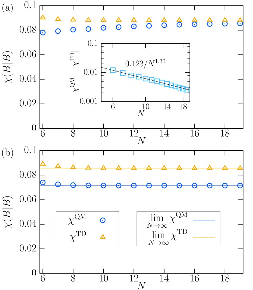
Figure 3: $\chi^{\text{QM}}_{N}(B|B)$ (blue circle) and $\chi^{\text{TD}}_{N}(B|B)$ (orange triangle) against the system size $N$ in (a) Model I (nonintegrable) and in (b) Model II (integrable). The solid lines in (b) show the thermodynamic limits of these susceptibilities. Inset of (a): A log-log plot of $N$ dependence of $|\chi^{\text{QM}}_{N}(B|B)-\chi^{\text{TD}}_{N}(B|B)|$ in Model I, which can be fitted by a function $a/N^{b}$ with constants $a=0.123(5)$, $b=1.30(2)$, and the solid line shows the fitting function $0.123/N^{1.30}$.

For comparison, we plot the two susceptibilities of Model II against $N$ in Fig. 3(b). The solid lines depict their thermodynamic limits, which are calculated from the analytic solutions (148) and (149) given in Appendix C. These results clearly show that Model II violates condition (36) and hence condition (19).

VII.3 Susceptibilities of $\hat{A}$

Next we calculate the susceptibilities of additive observables $\hat{A}$ that are not conjugate to the quench parameter $f=J_{zz}$ in order to demonstrate our Theorem (in the form rephrased in Sec. VI). That is, we demonstrate that Eq. (35) is satisfied for such $\hat{A}$’s in Model I while it is violated in Model II.

As typical $\hat{A}$’s, we choose the following observables for the demonstration. The first one is the sum of single-site observables,

$$\hat{M}^{x} :=\sum_{r=1}^{N}\hat{\sigma}_{r}^{x}.$$ (42)

The second one is the sum of two-spin observables,

$$\hat{M}^{xx} :=\sum_{r=1}^{N}\hat{\sigma}_{r}^{x}\hat{\sigma}_{r+1}^{x}.$$ (43)

The third one is also the sum of two-spin observables, but the two spins are the next nearest to each other,

$$\hat{M}^{z1z} :=\sum_{r=1}^{N}\hat{\sigma}_{r}^{z}\hat{\sigma}_{r+2}^{z},$$ (44)

where $\hat{\sigma}_{N+2}^{z}=\hat{\sigma}_{2}^{z}$.

The susceptibilities of $\hat{A}=\hat{M}^{x}$ of Model I are plotted against the system size $N$ in Fig. 4(a), and those of $\hat{A}=\hat{M}^{xx}$ and $\hat{M}^{z1z}$ are plotted in Figs. 5(a) and 6(a) of Appendix B, respectively. In each figure, $\chi^{\text{QM}}_{N}(A|B)$ and $\chi^{\text{TD}}_{N}(A|B)$ approach the same value with increasing $N$. The insets of these figures show the difference of the susceptibilities in a log-log plot. They indicate power law decays, as in the case of Fig. 3(a). From these results, we confirm that Eq. (35) is satisfied for all the three additive observables.

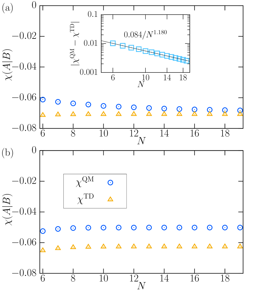
Figure 4: $\chi^{\text{QM}}_{N}(A|B)$ (blue circle) and $\chi^{\text{TD}}_{N}(A|B)$ (orange triangle) for $\hat{A}=\hat{M}^{x}$ against the system size $N$ in (a) Model I (nonintegrable) and in (b) Model II (integrable). Inset of (a): A log-log plot of $N$ dependence of $|\chi^{\text{QM}}_{N}(A|B)-\chi^{\text{TD}}_{N}(A|B)|$ in Model I, which can be fitted by a function $a/N^{b}$ with constants $a=0.084(2)$, $b=1.180(9)$, and the solid line shows the fitting function $0.084/N^{1.180}$.

For comparison, the susceptibilities of $\hat{A}=\hat{M}^{x}$, $\hat{M}^{xx}$, and $\hat{M}^{z1z}$ of Model II are plotted in Figs. 4(b), 5(b), and 6(b), respectively. In all these figures, $\chi^{\text{QM}}_{N}(A|B)$ and $\chi^{\text{TD}}_{N}(A|B)$ deviate from each other. Therefore we conclude that, in Model II, Eq. (35) is not satisfied for the three additive observables . This is consistent with our Theorem because this integrable model violates condition (36).

VIII Outlines of the proofs

In this section, we describe outlines of proofs of Theorem and Propositions of Secs. IV and V. A combination of these outlines and the detailed discussions in Appendix A gives the complete proofs.

VIII.1 Outline of the proof of Theorem

Since our Theorem in Sec. IV can be rephrased as the Consistency of cross responses of Sec. VI, we prove the latter.

It is known that the generalized susceptibilities can be expressed in terms of the canonical correlation [136, 186, 187], which is defined for arbitrary operators $\hat{X}$ and $\hat{Y}$ by

$$\langle\hat{X};\hat{Y}\rangle^{\text{eq}}_{0}:=\int_{0}^{1}\differential{\lambda}\Tr[(\hat{\rho}^{\text{eq}}_{0})^{1-\lambda}\hat{X}^{\dagger}(\hat{\rho}^{\text{eq}}_{0})^{\lambda}\hat{Y}\bigr{]}.$$ (45)

We start from such expressions. We then introduce an projection superoperator. We finally make use of the fact that the canonical correlation defines an inner product, i.e., it satisfies all of the axioms of an inner product (hence is called the Kubo-Mori-Bogoliubov inner product).

In Appendix A.1, we have expressed $\chi_{N}^{\text{QM}}(A|B)$ and $\chi^{\text{TD}}_{N}(A|B)$ using the canonical correlations as Eqs. (81) and  (84), respectively. These expressions yield

$$\chi^{\text{TD}}_{N}(A|B)-\chi^{\text{QM}}_{N}(A|B)$$

$$=\frac{1}{N}\langle\beta_{0}\delta\hat{B};\delta\overline{\hat{A}^{0}}\rangle^{\text{eq}}_{0}-\frac{\langle\beta_{0}\delta\hat{B}\delta\hat{H}_{0}\rangle^{\text{eq}}_{0}\langle\delta\hat{H}_{0}\delta\hat{A}\rangle^{\text{eq}}_{0}}{N\langle(\delta\hat{H}_{0})^{2}\rangle^{\text{eq}}_{0}},$$ (46)

where $\delta\hat{\bullet}:=\hat{\bullet}-\langle\hat{\bullet}\rangle^{\text{eq}}_{0}$ is the deviation from the initial equilibrium value, and we have introduced the Heisenberg operator,

$$\hat{X}^{0}(t):=e^{i\hat{H}_{0}t}\hat{X}e^{-i\hat{H}_{0}t},$$ (47)

and its long time average,

$$\overline{\hat{X}^{0}}:=\lim_{\mathcal{T}\to\infty}\overline{\hat{X}^{0}(t)}^{\mathcal{T}}.$$ (48)

Here, we have put the superscript $0$ because $\hat{X}^{0}(t)$ evolves by the initial Hamiltonian $\hat{H}_{0}$. Since $[\overline{\hat{X}^{0}},\hat{H}_{0}]=0$ holds for any operator $\hat{X}$, we can rewrite the first term of Eq. (46) as

$$\langle\delta\hat{B};\delta\overline{\hat{A}^{0}}\rangle^{\text{eq}}_{0}=\langle\delta\hat{B}\delta\overline{\hat{A}^{0}}\rangle^{\text{eq}}_{0}=\langle\delta\hat{B}^{0}(t)\delta\overline{\hat{A}^{0}}\rangle^{\text{eq}}_{0}$$

$$\quad=\langle\delta\overline{\hat{B}^{0}}\delta\overline{\hat{A}^{0}}\rangle^{\text{eq}}_{0}.$$ (49)

Now we introduce the following projection superoperator,

$$\mathcal{P}[\hat{X}]:=\delta\overline{\hat{X}^{0}}-\frac{\langle\delta\hat{H}_{0}\delta\overline{\hat{X}^{0}}\rangle^{\text{eq}}_{0}}{\langle(\delta\hat{H}_{0})^{2}\rangle^{\text{eq}}_{0}}\delta\hat{H}_{0}.$$ (50)

It projects an operator $\hat{X}$ onto the operator subspace whose elements (operators) commute with $\hat{H}_{0}$ and are orthogonal to $\hat{1}$ and $\hat{H}_{0}$ (under the Kubo-Mori-Bogoliubov inner product). By using this superoperator, Eq. (46) can be written as

$$\chi^{\text{TD}}_{N}(A|B)-\chi^{\text{QM}}_{N}(A|B) =\frac{\beta_{0}}{N}\langle\mathcal{P}[\hat{B}];\mathcal{P}[\hat{A}]\rangle^{\text{eq}}_{0}.$$ (51)

Since the r.h.s. is an inner product, we apply the Cauchy-Schwarz inequality, and obtain

$$|\chi^{\text{TD}}_{N}(A|B)-\chi^{\text{QM}}_{N}(A|B)|^{2}$$

$$\leq\frac{(\beta_{0})^{2}}{N^{2}}\langle\mathcal{P}[\hat{A}];\mathcal{P}[\hat{A}]\rangle^{\text{eq}}_{0}\langle\mathcal{P}[\hat{B}];\mathcal{P}[\hat{B}]\rangle^{\text{eq}}_{0}$$

$$=\Bigl{(}\chi^{\text{TD}}_{N}(A|A)-\chi^{\text{QM}}_{N}(A|A)\Bigr{)}\Bigl{(}\chi^{\text{TD}}_{N}(B|B)-\chi^{\text{QM}}_{N}(B|B)\Bigr{)}$$

$$\leq\chi^{\text{TD}}_{N}(A|A)\Bigl{(}\chi^{\text{TD}}_{N}(B|B)-\chi^{\text{QM}}_{N}(B|B)\Bigr{)},$$ (52)

where we have used $\chi^{\text{QM}}_{N}(A|A)\geq 0$, which follows from Eq. (81), and $\chi^{\text{TD}}_{N}(B|B)\geq\chi^{\text{QM}}_{N}(B|B)$ [137, 139], which is obvious from Eq. (51). Since we exclude phase transition points as stated in Sec. II, it is required that

$$\chi^{\text{TD}}_{N}(A|A)=\mathcal{O}(N^{0})\qquad\text{for any }\hat{A}$$ (53)

from thermodynamics and equilibrium statistical mechanics . Therefore, Eq. (52) yields the Consistency of cross responses of Sec. VI, and hence our Theorem in Sec. IV.

VIII.2 Outline of the proof of Proposition $1$

Let $|\nu\rangle$ be an eigenstate of $\hat{H}_{0}$ with an energy eigenvalue $E_{\nu}$. We take these eigenstates such that they form an orthonormal basis even if the eigenvalues are degenerate. The maximum number of resonances in condition (20) is defined by

$$D_{\text{res}}:=\max_{\nu_{1},\nu_{2}\ (E_{\nu_{1}}\neq E_{\nu_{2}})}\,\sum_{\nu_{3},\nu_{4}\ (E_{\nu_{3}}\neq E_{\nu_{4}})}\delta_{E_{\nu_{1}}-E_{\nu_{2}},E_{\nu_{3}}-E_{\nu_{4}}}.$$ (54)

As shown in Appendix A.2, the left hand side of Eq. (21) can be rewritten as

$$\lim_{\mathcal{T}\to\infty}\lim_{\Delta f\to 0}\overline{\biggl{|}\frac{\langle\hat{A}^{\Delta f}(t)\rangle^{\text{eq}}_{0}-\overline{\langle\hat{A}^{\Delta f}(t)\rangle^{\text{eq}}_{0}}^{\mathcal{T}}}{\Delta fN}\biggr{|}^{2}}^{\mathcal{T}}$$

$$\quad=\lim_{\mathcal{T}\to\infty}\overline{\bigl{(}\chi_{N}^{\text{QM}}(A|B;t)-\chi^{\text{QM}}_{N}(A|B)\bigr{)}^{2}}^{\mathcal{T}}.$$ (55)

Here $\chi_{N}^{\text{QM}}(A|B;t)$ is the time-dependent susceptibility,

$$\chi_{N}^{\text{QM}}(A|B;t) :=\lim_{\Delta f\to 0}\frac{\langle\hat{A}^{\Delta f}(t)\rangle^{\text{eq}}_{0}-\langle\hat{A}\rangle^{\text{eq}}_{0}}{N\Delta f},$$ (56)

which is related to $\chi^{\text{QM}}_{N}(A|B)$ via

$$\chi^{\text{QM}}_{N}(A|B)=\lim_{\mathcal{T}\to\infty}\overline{\chi_{N}^{\text{QM}}(A|B;t)}^{\mathcal{T}}.$$ (57)

The r.h.s. of Eq. (55) is bounded from above by

$$\lim_{\mathcal{T}\to\infty}\overline{\bigl{(}\chi_{N}^{\text{QM}}(A|B;t)-\chi^{\text{QM}}_{N}(A|B)\bigr{)}^{2}}^{\mathcal{T}}$$

$$\quad\leq\frac{(\beta_{0})^{2}\|\hat{A}\|_{\infty}^{2}\|\hat{B}\|_{\infty}^{2}}{N^{2}}D_{\text{res}}\Tr[(\hat{\rho}^{\text{eq}}_{0})^{2}\bigr{]}.$$ (58)

The proof of this inequality, shown in Appendix A.2, is similar to that by Short and Farrelly [146]. Combining Eqs. (55) and (58) with the condition (20), we prove Eq. (21) for every additive observable $\hat{A}$.

We remark that Eq. (58) can be extended to finite $\mathcal{T}$, as in Ref. [146].

VIII.3 Outline of the proof of Proposition 2

As explained in Appendix A.3, we can show that

$$\lim_{\Delta f\to 0}\frac{\text{Var}_{0}[\hat{A}^{\Delta f}(t)]-\text{Var}_{0}[\hat{A}]}{\Delta f}$$

$$\quad=\langle\beta_{0}\delta\hat{B};(\delta\hat{A})^{2}\rangle^{\text{eq}}_{0}-\langle\beta_{0}\delta\hat{B};\bigl{(}\delta\hat{A}^{0}(t)\bigr{)}^{2}\rangle^{\text{eq}}_{0},$$ (59)

where $\delta\hat{A}^{0}(t)=\hat{A}^{0}(t)-\langle\hat{A}^{0}(t)\rangle^{\text{eq}}_{0}=\hat{A}^{0}(t)-\langle\hat{A}\rangle^{\text{eq}}_{0}$. An upper bound of the last term is obtained by the Cauchy-Schwarz inequality as

$$\bigl{|}\langle\delta\hat{B};\bigl{(}\delta\hat{A}^{0}(t)\bigr{)}^{2}\rangle^{\text{eq}}_{0}\bigr{|}^{2}$$

$$\quad\leq\langle\delta\hat{B};\delta\hat{B}\rangle^{\text{eq}}_{0}\langle\bigl{(}\delta\hat{A}^{0}(t)\bigr{)}^{2};\bigl{(}\delta\hat{A}^{0}(t)\bigr{)}^{2}\rangle^{\text{eq}}_{0}$$

$$\quad=\langle\delta\hat{B};\delta\hat{B}\rangle^{\text{eq}}_{0}\langle(\delta\hat{A})^{2};(\delta\hat{A})^{2}\rangle^{\text{eq}}_{0}$$

$$\quad\leq\langle(\delta\hat{B})^{2}\rangle^{\text{eq}}_{0}\langle(\delta\hat{A})^{4}\rangle^{\text{eq}}_{0}.$$ (60)

Here the last line follows from Eq. (105) of Appendix A.3. By using this inequality, we have

$$\lim_{\Delta f\to 0} \left|\frac{\text{Var}_{0}[\hat{A}^{\Delta f}(t)]-\text{Var}_{0}[\hat{A}]}{\Delta f}\right|$$

$$\leq 2\beta_{0}\sqrt{\langle(\delta\hat{B})^{2}\rangle^{\text{eq}}_{0}\langle(\delta\hat{A})^{4}\rangle^{\text{eq}}_{0}}.$$ (61)

Since the time average of the left-hand side (l.h.s.) of this inequality can also be bounded from above by the same quantity, we have

$$\lim_{\mathcal{T}\to\infty}\lim_{\Delta f\to 0}\left|\frac{\overline{\text{Var}_{0}[\hat{A}^{\Delta f}(t)]}^{\mathcal{T}}-\text{Var}_{0}[\hat{A}]}{\Delta f}\right|$$

$$\qquad\leq 2\beta_{0}\sqrt{\langle(\delta\hat{B})^{2}\rangle^{\text{eq}}_{0}\langle(\delta\hat{A})^{4}\rangle^{\text{eq}}_{0}}.$$ (62)

Here, we have used interchangeability of the time integration and the limit $\Delta f\to 0$, which is shown in Eqs. (122)–(124) of Appendix A.4. Combining this with the condition (23) and its consequence (25), we obtain Eq. (24).

It should be remarked that Eq. (61) holds at an arbitrary time $t>0$ without taking time average. That is, the variance remains small at all $t>0$, although Criterion (iii) requires it only for almost all $t>0$.

VIII.4 Outline of the proof of Proposition 3

We use the following inequalities that are proved in Appendix A.4,

$$\Bigl{|}\frac{\overline{\langle\hat{A}^{\Delta f}(t)\rangle^{\text{eq}}_{0}}^{\mathcal{T}}-\langle\hat{A}\rangle^{\text{eq}}_{0}}{\Delta fN}-\overline{\chi_{N}^{\text{QM}}(A|B;t)}^{\mathcal{T}}\Bigr{|}$$

$$\leq\bigl{(}D_{1}\mathcal{T}+D_{2}\mathcal{T}^{2}\bigr{)}|\Delta f|,$$ (63)

$$\Bigl{|}\overline{\Bigl{(}\frac{\langle\hat{A}^{\Delta f}(t)\rangle^{\text{eq}}_{0}-\langle\hat{A}\rangle^{\text{eq}}_{0}}{\Delta fN}\Bigr{)}^{2}}^{\mathcal{T}}-\overline{\bigl{(}\chi_{N}^{\text{QM}}(A|B;t)\bigr{)}^{2}}^{\mathcal{T}}\Bigr{|}$$

$$\leq\bigl{(}D_{3}\mathcal{T}+D_{4}\mathcal{T}^{2}\bigr{)}|\Delta f|$$

$$\qquad+\bigl{(}D_{5}\mathcal{T}^{2}+D_{6}\mathcal{T}^{3}+D_{7}\mathcal{T}^{4}\bigr{)}|\Delta f|^{2},$$ (64)

$$\Bigl{|}\frac{\overline{\langle\bigl{(}\hat{A}^{\Delta f}(t)\bigr{)}^{2}\rangle^{\text{eq}}_{0}}^{\mathcal{T}}-\langle\hat{A}^{2}\rangle^{\text{eq}}_{0}}{\Delta fN^{2}}-\overline{\tilde{\chi}_{N}(A^{2};t)}^{\mathcal{T}}\Bigr{|}$$

$$\leq\bigl{(}D_{8}\mathcal{T}+D_{9}\mathcal{T}^{2}\bigr{)}|\Delta f|.$$ (65)

Here

$$\tilde{\chi}_{N}(A^{2};t):=\lim_{\Delta f\to 0}\frac{\langle\bigl{(}\hat{A}^{\Delta f}(t)\bigr{)}^{2}\rangle^{\text{eq}}_{0}-\langle\hat{A}^{2}\rangle^{\text{eq}}_{0}}{\Delta fN^{2}},$$ (66)

and $D_{1},\cdots,D_{9}$ are nonnegative constants of $\mathcal{O}(|\Delta f|^{0})$ that are independent of $\mathcal{T}$. By noting that the right-hand sides of these equations vanish in the limit (28), we can prove Eqs. (29)–(31) as follows.

Firstly, combining Eq. (63) with Eq. (57), we have

$$\lim_{\Delta f\to 0}\frac{\overline{\langle\hat{A}^{\Delta f}(t)\rangle^{\text{eq}}_{0}}^{\mathcal{T}_{\Delta f}}-\langle\hat{A}\rangle^{\text{eq}}_{0}}{\Delta fN}=\chi_{N}^{\text{QM}}(A|B).$$ (67)

Using Eqs. (33), (34) and (67), we obtain Eq. (29).

Next we evaluate

$$\overline{\biggl{|}\frac{\langle\hat{A}^{\Delta f}(t)\rangle^{\text{eq}}_{0}-\overline{\langle\hat{A}^{\Delta f}(t)\rangle^{\text{eq}}_{0}}^{\mathcal{T}}}{\Delta fN}\biggr{|}^{2}}^{\mathcal{T}}$$

$$=\overline{\Bigl{(}\frac{\langle\hat{A}^{\Delta f}(t)\rangle^{\text{eq}}_{0}-\langle\hat{A}\rangle^{\text{eq}}_{0}}{\Delta fN}\Bigr{)}^{2}}^{\mathcal{T}}-\Bigl{(}\frac{\overline{\langle\hat{A}^{\Delta f}(t)\rangle^{\text{eq}}_{0}}^{\mathcal{T}}-\langle\hat{A}\rangle^{\text{eq}}_{0}}{\Delta fN}\Bigr{)}^{2}.$$ (68)

By taking the limit (28), we can evaluate the first and second terms from Eqs. (64) and (67), respectively. Then we have

$$\lim_{\Delta f\to 0}\overline{\biggl{|}\frac{\langle\hat{A}^{\Delta f}(t)\rangle^{\text{eq}}_{0}-\overline{\langle\hat{A}^{\Delta f}(t)\rangle^{\text{eq}}_{0}}^{\mathcal{T}_{\Delta f}}}{\Delta fN}\biggr{|}^{2}}^{\mathcal{T}_{\Delta f}}$$

$$=\lim_{\mathcal{T}\to\infty}\overline{\bigl{(}\chi_{N}^{\text{QM}}(A|B;t)\bigr{)}^{2}}^{\mathcal{T}}-\bigl{(}\chi^{\text{QM}}_{N}(A|B)\bigr{)}^{2}.$$ (69)

Combining this with Eq. (55), we obtain Eq. (30).

Finally we evaluate

$$\frac{\overline{\text{Var}_{0}[\hat{A}^{\Delta f}(t)]}^{\mathcal{T}}-\text{Var}_{0}[\hat{A}]}{\Delta fN^{2}}$$

$$=\frac{\overline{\langle\bigl{(}\hat{A}^{\Delta f}(t)\bigr{)}^{2}\rangle^{\text{eq}}_{0}}^{\mathcal{T}}-\langle\hat{A}^{2}\rangle^{\text{eq}}_{0}}{\Delta fN^{2}}-\overline{\Bigl{(}\frac{\langle\hat{A}^{\Delta f}(t)\rangle^{\text{eq}}_{0}-\langle\hat{A}\rangle^{\text{eq}}_{0}}{\Delta fN}\Bigr{)}^{2}\Delta f}^{\mathcal{T}}$$

$$\qquad-2\frac{\langle\hat{A}\rangle^{\text{eq}}_{0}}{N}\frac{\overline{\langle\hat{A}^{\Delta f}(t)\rangle^{\text{eq}}_{0}}^{\mathcal{T}}-\langle\hat{A}\rangle^{\text{eq}}_{0}}{\Delta fN}$$ (70)

By taking the limit (28), we can evaluate the first and third terms from Eqs. (65) and (67), respectively. Note that the second term vanishes in this limit because of Eq. (64). As a result, we have

$$\lim_{\Delta f\to 0}\frac{\overline{\text{Var}_{0}[\hat{A}^{\Delta f}(t)]}^{\mathcal{T}_{\Delta f}}-\text{Var}_{0}[\hat{A}]}{\Delta fN^{2}}$$

$$=\lim_{\mathcal{T}\to\infty}\overline{\tilde{\chi}_{N}(A^{2};t)}^{\mathcal{T}}-2\frac{\langle\hat{A}\rangle^{\text{eq}}_{0}}{N}\chi^{\text{QM}}_{N}(A|B)$$

$$=\lim_{\mathcal{T}\to\infty}\overline{\Bigl{(}\lim_{\Delta f\to 0}\frac{\text{Var}_{0}[\hat{A}^{\Delta f}(t)]-\text{Var}_{0}[\hat{A}]}{\Delta fN^{2}}\Bigr{)}}^{\mathcal{T}}.$$ (71)

In the last line, we have used

$$\lim_{\Delta f\to 0}\frac{\text{Var}_{0}[\hat{A}^{\Delta f}(t)]-\text{Var}_{0}[\hat{A}]}{\Delta fN^{2}}$$

$$=\tilde{\chi}_{N}(A^{2};t)-2\frac{\langle\hat{A}\rangle^{\text{eq}}_{0}}{N}\chi^{\text{QM}}_{N}(A|B;t),$$ (72)

which follows from Eqs. (101) and (102) of Appendix A.3. From Eqs. (122)–(124) of Appendix A.4, the time integration and the limit $\Delta f\to 0$ can be interchanged, and hence Eq. (71) yields Eq. (31).

IX Discussions

IX.1 Extension to nonadditive observables

In the above proof, additivity of $\hat{A}$ and $\hat{B}$ is not crucial. In fact, we can extend our Theorem as follows.
Extension to nonadditive observables: Suppose that the observable $\hat{B}$ defined by Eq. (10) is not necessarily additive. If Eq. (18) holds for $\hat{B}$ then it holds for any observable $\hat{A}$ that is not necessarily additive but satisfies

$$\chi^{\text{TD}}_{N}(A|A)-\chi^{\text{QM}}_{N}(A|A)=\mathcal{O}(N^{0}).$$ (73)

This result will be particularly useful when discussing nonlocal properties of the system, such as the entanglement. Nevertheless, we have focused on additive observables because we are interested in consistency with thermodynamics in this paper.

IX.2 Case of continuous change of $f$

We have studied the case of a quench process, in which $f$ is jumped discontinuously. Our Theorem holds also for processes in which $f$ is changed continuously as

$$f(t)=f_{0}+\lambda(t)\Delta f.$$ (74)

Here, $\lambda(t)$ is a continuously differentiable function such that $\lambda(t)=0$ for $t\leq 0$ and $\lambda(t)=1$ for $t^{*}\leq t$, where $t^{*}$ is a constant independent of $\Delta f$ and $\mathcal{T}$.

The validity of our Theorem for this process is shown as follows. $\chi^{\text{QM}}_{N}(A|B)$ of this process agrees with that of the quench process because $\chi^{\text{QM}}_{N}(A|B)$ is the zero-frequency component of a linear-response coefficient and hence independent of the time profile of $f$, as will be shown in Sec. IX.5. $\chi^{\text{TD}}_{N}(A|B)$ is also independent of the time profile of $f$ because it agrees with the adiabatic susceptibility regardless of the time profile of $f$. In fact, the entropy does not change in $\mathcal{O}(\Delta f)$ because if the entropy increased by $\mathcal{O}(\Delta f)$ then it would decrease when the sign of $\Delta f$ is inverted, in contradiction to the second law of thermodynamics. Therefore, our Theorem holds independently of details of the process.

IX.3 ETH for $\hat{B}$ implies condition (19) but they are inequivalent

In this subsection, we show that the ETH for $\hat{B}$ implies condition (19) but the converse is not necessarily true.

In Ref. [135], we have shown that if the ETH (referred to as the “strong ETH” there) is satisfied for the uniform magnetization then condition (8) of Ref. [135] holds. This condition is equivalent to Eq. (4) of Ref. [135], which states that the ${\bf\it k}={\bf\it 0}$ components of two types of magnetic susceptibilities, denoted by $\chi^{\text{qch}}_{N}({\bf\it 0})$ and $\chi^{S}_{N}({\bf\it 0})$ there, coincide. We can easily show that the proof is applicable when $\chi^{\text{qch}}_{N}({\bf\it 0})$ and $\chi^{S}_{N}({\bf\it 0})$ are replaced with the generalized susceptibilities $\chi^{\text{QM}}_{N}(\hat{B}|\hat{B})$ and $\chi^{\text{TD}}_{N}(\hat{B}|\hat{B})$ introduced in Sec. VI, respectively, and the uniform magnetization with $\hat{B}$. Therefore, the ETH for $\hat{B}$ implies Eq. (36) of the present paper, which is equivalent to condition (19) as explained in Sec. VI.

Note that this result is not so obvious because, as shown in Sec. V, the timescale of linear thermalization in condition (19) is shorter than the timescale where the ETH is usually applied. In other words, when applying the ETH, one usually take $\mathcal{T}\to\infty$ before $\Delta f\to 0$, which differs from the limit (27) employed in condition (19).

On the other hand, condition (19) for $\hat{B}$ is weaker than its ETH. In fact, Shiraishi and Mori [24, 25] constructed systems in which a certain observable violates the ETH but satisfies Criterion (i) when the initial state is an arbitrary equilibrium state at a nonzero temperature. Hence, when $f$ is chosen as the parameter conjugate to that observable, these systems satisfy condition (19) but violate the ETH for $\hat{B}$.

IX.4 How to test our results experimentally

In this section, we discuss a way of testing our results experimentally. For concreteness, we discuss how to measure $\chi_{N}^{\text{QM}}(A|B)$ and $\chi_{N}^{\text{TD}}(A|B)$. Other quantities such as fluctuation can also be measured in a similar manner.

To measure $\chi_{N}^{\text{QM}}(A|B)$ experimentally, prepare the system in an equilibrium state . This can be achieved, for example, by making the system be in thermal contact with a heat bath of inverse temperature $\beta_{0}$. Obtain $\langle\hat{A}\rangle^{\text{eq}}_{0}$ by measuring $\hat{A}$ in this state. After that, detach the heat bath, so that the system undergoes the unitary time evolution. Then, $\langle\hat{A}^{\Delta f}(t)\rangle^{\text{eq}}_{0}$ evolves as schematically shown in Fig. 1. By measuring this evolution, one can judge whether the system relaxes to a (quasi)-steady state or not. Note that the (quasi)-steady state can be a nonthermal state because the relaxation occurs much more easily than thermalization, as pointed out at the beginning of Sec. IV. When the relaxation occurs, one obtains $\overline{\langle\hat{A}^{\Delta f}(t)\rangle^{\text{eq}}_{0}}^{\mathcal{T}}$ and the relaxation time. By taking $|\Delta f|$ small enough and $\mathcal{T}$ long enough , and extrapolating the data to $\Delta f\to 0$ and $\mathcal{T}\to\infty$, one obtains $\chi_{N}^{\text{QM}}(A|B)$ as Eq. (33). One also obtains the $\Delta f$ dependence of the relaxation time from the $\Delta f$ dependence of the data.

For $\chi_{N}^{\text{TD}}(A|B)$, its measurement might look difficult when the system does not thermalize under the unitary evolution. Fortunately, one can fully utilize a heat bath to realize equilibrium states because $\chi_{N}^{\text{TD}}(A|B)$ is a state function and therefore independent [apart from a finite-size-effect term of $o(N^{0})$] of how the equilibrium state is prepared. Firstly, set $f=f_{0}$ and $\beta=\beta_{0}$, and obtain $\langle\hat{A}\rangle^{\text{eq}}_{0}$ by measuring $\hat{A}$. Then, supply a small amount of energy $dU$ to the total system (composed of the system and the bath), and measure the resultant decrease $d\beta$ of the inverse temperature and the change $dB$ of the equilibrium value of $\hat{B}$. Since the thermal capacity of the bath is known, one obtains the specific heat $c_{0}$ of the system from $dU$ and $d\beta$. Furthermore, $dB/d\beta$ gives

$$\evaluated{\Bigl{(}\partialderivative{\beta}\Tr[\hat{\rho}^{\text{can}}(\beta,f_{0})\frac{\hat{B}}{N}\Bigr{]}\Bigr{)}}_{\beta=\beta_{0}}=-\langle\delta\hat{H}_{0}\delta\hat{B}\rangle^{\text{eq}}_{0}/N.$$ (75)

Then, using this and Eq. (83), one can determine the inverse temperature $\beta_{\Delta f}$, given by Eq. (82), of the final equilibrium state that is predicted by thermodynamics after the quench of $\Delta f$ . Finally, set $f=f_{0}+\Delta f$ and $\beta=\beta_{\Delta f}$, and obtain $\langle\hat{A}\rangle^{\text{eq}}_{\Delta f}$ by measuring $\hat{A}$. By substituting the measured values for $\langle\hat{A}\rangle^{\text{eq}}_{0}$ and $\langle\hat{A}\rangle^{\text{eq}}_{\Delta f}$ of Eq. (34), one obtains $\chi_{N}^{\text{TD}}(A|B)$.

IX.5 Relation to linear response theory

The quantum-mechanical susceptibility, $\chi_{N}^{\text{QM}}(A|B)$, is closely related to that given by the linear response theory. Hence, the consistency of $\chi_{N}^{\text{QM}}(A|B)$ with $\chi_{N}^{\text{TD}}(A|B)$, discussed in Sec. VI, is also related to the validity of the linear response theory. We finally discuss these points.

Following the pioneering studies by Callen, Welton, Greene, Takahashi, and Nakano [192, 193, 194, 195, 196], Kubo established the linear response theory for quantum systems  [136]. He assumed that the system, which is initially in an equilibrium state, is isolated from environments while an external force is applied adiabatically, which means, in our notation, that

$$f(t)=f_{0}+\Delta fe^{\varepsilon t}\cos\omega t.$$ (76)

Here $\varepsilon$ is a small positive number and $\omega$ is the frequency. Then, the Kubo formula for the response of $\hat{A}/N$ reads

$$\chi_{N}^{\text{Kubo}}(A|B)[\omega+i\varepsilon]=\int_{0}^{\infty}\differential{t}e^{(i\omega-\varepsilon)t}\frac{i}{N}\langle[\hat{A}^{0}(t),\hat{B}]\rangle^{\text{eq}}_{0},$$ (77)

where $\hat{A}^{0}(t)$ is defined by Eq. (47).

Note that the validity of this formula is never obvious because it depends on the degree of complexity of the dynamics. The conditions for the validity have been discussed by Kubo himself [136] and by many authors [186, 137, 139, 135]. For technical reasons, these discussions have been made for finite $N$, although it is sometimes stressed that the thermodynamic limit should be taken before taking other limits such as $\varepsilon\to+0$ [197, 198, 199, 200, 201].

If we keep $N$ finite following these studies, we can show that [135]

$$\lim_{\varepsilon\to+0}\chi_{N}^{\text{Kubo}}(A|B)[0+i\varepsilon]=\chi_{N}^{\text{QM}}(A|B).$$ (78)

Therefore, the validity of the Kubo formula can be judged from the validity of $\chi_{N}^{\text{QM}}(A|B)$, which was discussed in Sec. VI. That is, the validity for the response of the key observable against $\Delta f$ guarantees the validity for those of other observables and for the responses against any other parameters. By contrast, the previous conditions for the validity [136, 186, 137, 139, 135] required investigations of individual observables and responses.

It is worth mentioning that the above validity means the agreement of the response between quantum mechanics and thermodynamics. On the other hand, the classical limit of Eq. (77) yields the “fluctuation-dissipation theorem” (FDT). It states that

$$[\mbox{response at $\omega$}]=\beta\times[\mbox{correlation spectrum at $\omega$}],$$ (79)

where the r.h.s. is not a formal one but the observed spectrum. In classical systems the FDT, despite its name, holds even for non-dissipative responses [195]. Many authors discussed its quantum corrections [202, 192, 196, 136, 186, 203, 204, 205, 206, 207, 208, 209, 210]. Although their results partially disagree with each other, it can be interpreted as due to different assumptions on the ways of measurements. However, it is recently shown rigorously that the observed fluctuation in macroscopic systems is independent of details of the ways of measurements when the measurement is performed as ideally as possible [211, 212]. This universal result clarified when the FDT [in the form of Eq. (79)] holds and when it is violated [211, 212, 213, 214].

These studies on the FDT also demonstrate that the nonequilibrium statistical mechanics is never trivial even in the linear response regime.

X Summary

We have studied how quantum mechanics is consistent with thermodynamics with respect to infinitesimal transitions between equilibrium states. We suppose that an isolated quantum many-body system is prepared in an equilibrium state, and then a parameter $f$ of the Hamiltonian is changed by a small amount $\Delta f$, which induces the unitary time evolution. By inspecting the expectation values and the variances of all additive observables, we have investigated whether linear thermalization occurs, i.e., whether the system relaxes to the equilibrium state that is fully consistent with thermodynamics up to the linear order in $\Delta f$.

By comparing the long time average of the expectation value of an arbitrary additive observable $\hat{A}$ with its equilibrium value predicted by thermodynamics, we have obtained Theorem described in Sec. IV.1. It states roughly that the two values coincide for every $\hat{A}$ if and only if they coincide for a single additive observable. This key observable is identified as the additive observable $\hat{B}$ that is conjugate to $f$. We have also pointed out that this condition for $\hat{B}$ is weaker than the ETH for $\hat{B}$.

To reinforce Theorem, we have then proved two propositions. Proposition 1, described in Sec. IV.2, shows that the time fluctuation of the expectation value (after changing $f$) is macroscopically negligible for every $\hat{A}$ as long as the number of resonating pairs of energy eigenvalues (before changing $f$) is not exponentially large. Proposition 2, described in Sec. IV.3, shows that the variances of all $\hat{A}$’s remain macroscopically negligible if fluctuations of $\hat{A}$’s in the initial equilibrium state have reasonable magnitudes as Eq. (23). Reinforced with these propositions, Theorem ensures that, under the reasonable conditions, the linear thermalization of the key observable $\hat{B}$ implies linear thermalization of all additive observables, which means full consistency with thermodynamics.

We have also proved Proposition 3 in Sec. V, which extends the above theorem and propositions to a longer timescale. It show that when linear thermalization occurs, it occurs in a timescale that is independent of the magnitude of $\Delta f$, $t=\mathcal{O}(|\Delta f|^{0})$, and it lasts at least for a period not shorter than $o(1/\sqrt{|\Delta f|})$. On the other hand, when linear thermalization does not occur by $t=\mathcal{O}(|\Delta f|^{0})$, it does not occur at least in a period of $o(1/\sqrt{|\Delta f|})$.

Furthermore, we have shown that Theorem has significant meanings about the generalized susceptibilities for cross responses, which have been attracting much attention in condensed matter physics. Theorem guarantees that the quantum-mechanical susceptibility of every additive observable $\hat{A}$ coincides with the thermodynamical one if those of the key observable $\hat{B}$ coincide. We have also obtained two corollaries, described in Sec. VI, about response of $\hat{B}$ to another parameter $f_{A}$ that is conjugate to an arbitrary additive observable $\hat{A}$. Corollary 1 states that the quantum-mechanical susceptibility of $\hat{B}$ to $f_{A}$ and the thermodynamical one coincide if those of $\hat{B}$ to its own conjugate parameter $f$ coincide. This is rephrased in terms of linear thermalization as Corollary 2: Linear thermalization of $\hat{B}$ against $\Delta f$ implies linear thermalization of $\hat{B}$ against any other $\Delta f_{A}$.

We have demonstrated Theorem by numerically calculating the generalized susceptibilities in three models. In a nonintegrable model, we have first shown linear thermalization of $\hat{B}$, and then confirmed that of other $\hat{A}$’s predicted by Theorem. We have also studied two integrable models; one can be mapped to noninteracting fermions, the other is solvable by the Bethe ansatz. We have found that linear thermalization does not occur either for $\hat{B}$ or for other $\hat{A}$’s in these models. This is again consistent with Theorem.

Our results will dramatically reduce the costs of experiments and theoretical calculations of linear thermalization and cross responses because testing them for a single key observable against the change of its conjugate parameter in a timescale of $\mathcal{O}(|\Delta f|^{0})$ gives much information about those for all additive observables, about those against the changes of any other parameters, and about a longer timescale.

Appendix A Derivation of relations used in proofs

A.1 Relations used in proof of Theorem

From the linear response theory [136, 186, 137, 139], the time-dependent quantum-mechanical susceptibility defined by Eq. (56) can be written as

$$\chi_{N}^{\text{QM}}(A|B;t)$$

$$=\frac{1}{N}\langle\beta_{0}\delta\hat{B};\delta\hat{A}\rangle^{\text{eq}}_{0}-\frac{1}{N}\langle\beta_{0}\delta\hat{B};\delta\hat{A}^{0}(t)\rangle^{\text{eq}}_{0},$$ (80)

which results in

$$\chi_{N}^{\text{QM}}(A|B)$$

$$=\frac{1}{N}\langle\beta_{0}\delta\hat{B};\delta\hat{A}\rangle^{\text{eq}}_{0}-\frac{1}{N}\langle\beta_{0}\delta\hat{B};\delta\overline{\hat{A}^{0}}\rangle^{\text{eq}}_{0}.$$ (81)

For $\chi^{\text{TD}}_{N}(A|B)$, we obtain $\beta_{\Delta f}$ from energy conservation, Eq. (15), as

$$\beta_{\Delta f}-\beta_{0}=-\frac{\langle\beta_{0}\delta\hat{B}\delta\hat{H}_{0}\rangle^{\text{eq}}_{0}}{\langle(\delta\hat{H}_{0})^{2}\rangle^{\text{eq}}_{0}}\Delta f+o(\Delta f).$$ (82)

Here, since $(\beta_{0},f_{0})$ is not at a phase transition point, the specific heat

$$c_{0}:=\beta_{0}^{2}\frac{\langle(\delta\hat{H}_{0})^{2}\rangle^{\text{eq}}_{0}}{N}$$ (83)

takes a positive finite value for sufficiently large $N$, $c_{0}=\Theta(N^{0})$. By substituting Eq. (82) into Eq. (34), we have

$$\chi_{N}^{\text{TD}}(A|B)$$

$$=\frac{1}{N}\langle\beta_{0}\delta\hat{B};\delta\hat{A}\rangle^{\text{eq}}_{0}-\frac{\langle\beta_{0}\delta\hat{B}\delta\hat{H}_{0}\rangle^{\text{eq}}_{0}\langle\delta\hat{H}_{0}\delta\hat{A}\rangle^{\text{eq}}_{0}}{N\langle(\delta\hat{H}_{0})^{2}\rangle^{\text{eq}}_{0}}.$$ (84)

A.2 Relations used in proof of Proposition $1$

We derive Eqs. (55), (58) and (22).

First, we derive Eq. (55). The temporal fluctuation of $\langle\hat{A}^{\Delta f}(t)\rangle^{\text{eq}}_{0}$ can be divided into two terms,

$$\overline{\biggl{|}\frac{\langle\hat{A}^{\Delta f}(t)\rangle^{\text{eq}}_{0}-\overline{\langle\hat{A}^{\Delta f}(t)\rangle^{\text{eq}}_{0}}^{\mathcal{T}}}{\Delta fN}\biggr{|}^{2}}^{\mathcal{T}}$$

$$=\overline{\biggl{|}\frac{\langle\hat{A}^{\Delta f}(t)\rangle^{\text{eq}}_{0}-\langle\hat{A}\rangle^{\text{eq}}_{0}}{\Delta fN}\biggr{|}^{2}}^{\mathcal{T}}-\biggl{|}\frac{\overline{\langle\hat{A}^{\Delta f}(t)\rangle^{\text{eq}}_{0}}^{\mathcal{T}}-\langle\hat{A}\rangle^{\text{eq}}_{0}}{\Delta fN}\biggr{|}^{2}.$$ (85)

We evaluate these two terms in the limit $\Delta f\to 0$. The first term will be evaluated in Appendix A.4 as Eq. (123). From Eq. (122), which will also be given in Appendix A.4, the second term is evaluated as

$$\lim_{\Delta f\to 0}\biggl{|}\frac{\overline{\langle\hat{A}^{\Delta f}(t)\rangle^{\text{eq}}_{0}}^{\mathcal{T}}-\langle\hat{A}\rangle^{\text{eq}}_{0}}{\Delta fN}\biggr{|}^{2}=\Bigl{(}\overline{\chi_{N}^{\text{QM}}(A|B;t)}^{\mathcal{T}}\Bigr{)}^{2}.$$ (86)

Therefore, Eq. (85) is evaluated, in the limit $\Delta f\to 0$, as

$$\lim_{\Delta f\to 0}\overline{\biggl{|}\frac{\langle\hat{A}^{\Delta f}(t)\rangle^{\text{eq}}_{0}-\overline{\langle\hat{A}^{\Delta f}(t)\rangle^{\text{eq}}_{0}}^{\mathcal{T}}}{\Delta fN}\biggr{|}^{2}}^{\mathcal{T}}$$

$$=\overline{\Bigl{(}\chi_{N}^{\text{QM}}(A|B;t)-\overline{\chi_{N}^{\text{QM}}(A|B;t)}^{\mathcal{T}}\Bigr{)}^{2}}^{\mathcal{T}}$$

$$=\overline{\bigl{(}\chi_{N}^{\text{QM}}(A|B;t)-\chi^{\text{QM}}_{N}(A|B)\bigr{)}^{2}}^{\mathcal{T}}$$

$$\quad-\Bigl{(}\overline{\chi_{N}^{\text{QM}}(A|B;t)}^{\mathcal{T}}-\chi^{\text{QM}}_{N}(A|B)\Bigr{)}^{2}.$$ (87)

By taking the limit $\mathcal{T}\to\infty$, we obtain Eq. (55).

Next, we derive Eq. (58). Using Eqs. (45), (80), (81) and the eigenstates of $\hat{H}_{0}$, we have

$$\chi_{N}^{\text{QM}}(A|B;t)-\chi^{\text{QM}}_{N}(A|B)$$

$$=\frac{1}{N}\langle\beta_{0}\delta\hat{B};\delta\overline{\hat{A}^{0}}\rangle^{\text{eq}}_{0}-\frac{1}{N}\langle\beta_{0}\delta\hat{B};\delta\hat{A}^{0}(t)\rangle^{\text{eq}}_{0}$$

$$=-\sum_{\nu_{1},\nu_{2}(E_{\nu_{1}}\neq E_{\nu_{2}})}\frac{\beta_{0}}{N}\int_{0}^{1}\differential{\lambda}\rho_{\nu_{1}}^{1-\lambda}\langle\nu_{1}|\hat{B}|\nu_{2}\rangle\rho_{\nu_{2}}^{\lambda}\matrixelement{\nu_{2}}{\hat{A}}{\nu_{1}}$$

$$\hskip 110.0pt\times e^{-i(E_{\nu_{1}}-E_{\nu_{2}})t},$$ (88)

where

$$\rho_{\nu}:=e^{-\beta_{0}E_{\nu}}/Z(\beta_{0},f_{0})$$ (89)

and we have used

$$\overline{\hat{A}^{0}}=\sum_{\nu_{1},\nu_{2}\ (E_{\nu_{1}}=E_{\nu_{2}})}\ket{\nu_{1}}\matrixelement{\nu_{1}}{\hat{A}}{\nu_{2}}\bra{\nu_{2}}.$$ (90)

Hence we have

$$\chi_{N}^{\text{QM}}(A|B;t)-\chi^{\text{QM}}_{N}(A|B)$$

$$=-\sum_{\nu_{1},\nu_{2}\ (E_{\nu_{1}}\neq E_{\nu_{2}})}\frac{1}{N}\frac{\rho_{\nu_{2}}-\rho_{\nu_{1}}}{E_{\nu_{1}}-E_{\nu_{2}}}\langle\nu_{1}|\hat{B}|\nu_{2}\rangle\langle\nu_{2}|\hat{A}|\nu_{1}\rangle$$

$$\hskip 110.0pt\times e^{-i(E_{\nu_{1}}-E_{\nu_{2}})t}$$

$$=-\sum_{\nu_{1},\nu_{2}\ (E_{\nu_{1}}\neq E_{\nu_{2}})}v_{(\nu_{1},\nu_{2})}e^{-i(E_{\nu_{1}}-E_{\nu_{2}})t},$$ (91)

where, for $E_{\nu_{1}}\neq E_{\nu_{2}}$, we have introduced

$$v_{(\nu_{1},\nu_{2})} :=\frac{1}{N}\frac{\rho_{\nu_{2}}-\rho_{\nu_{1}}}{E_{\nu_{1}}-E_{\nu_{2}}}\langle\nu_{1}|\hat{B}|\nu_{2}\rangle\langle\nu_{2}|\hat{A}|\nu_{1}\rangle$$ (92)

$$=v_{(\nu_{2},\nu_{1})}^{*}.$$ (93)

Using this expression, the time fluctuation of $\chi_{N}^{\text{QM}}(A|B;t)$ is evaluated as

$$\lim_{\mathcal{T}\to\infty}\overline{\bigl{(}\chi_{N}^{\text{QM}}(A|B;t)-\chi^{\text{QM}}_{N}(A|B)\bigr{)}^{2}}^{\mathcal{T}}$$

$$=\sum_{(\nu_{1},\nu_{2})\in\mathcal{G}}\sum_{(\nu_{3},\nu_{4})\in\mathcal{G}}v_{(\nu_{3},\nu_{4})}^{*}v_{(\nu_{1},\nu_{2})}$$

$$\hskip 80.0pt\times\lim_{\mathcal{T}\to\infty}\overline{e^{i(E_{\nu_{3}}-E_{\nu_{4}}-E_{\nu_{1}}+E_{\nu_{2}})t}}^{\mathcal{T}}$$

$$=\sum_{(\nu_{1},\nu_{2})\in\mathcal{G}}\sum_{(\nu_{3},\nu_{4})\in\mathcal{G}}v_{(\nu_{3},\nu_{4})}^{*}v_{(\nu_{1},\nu_{2})}\delta_{E_{\nu_{1}}-E_{\nu_{2}},E_{\nu_{3}}-E_{\nu_{4}}}.$$ (94)

By using $|v_{(\nu_{3},\nu_{4})}^{*}v_{(\nu_{1},\nu_{2})}|\leq(|v_{(\nu_{3},\nu_{4})}|^{2}+|v_{(\nu_{1},\nu_{2})}|^{2})/2$, we have

$$\lim_{\mathcal{T}\to\infty}\overline{\bigl{(}\chi_{N}^{\text{QM}}(A|B;t)-\chi^{\text{QM}}_{N}(A|B)\bigr{)}^{2}}^{\mathcal{T}}$$

$$\leq\sum_{(\nu_{1},\nu_{2})\in\mathcal{G}}|v_{(\nu_{1},\nu_{2})}|^{2}\sum_{(\nu_{3},\nu_{4})\in\mathcal{G}}\delta_{E_{\nu_{1}}-E_{\nu_{2}},E_{\nu_{3}}-E_{\nu_{4}}}$$

$$\leq D_{\text{res}}\sum_{(\nu_{1},\nu_{2})\in\mathcal{G}}|v_{(\nu_{1},\nu_{2})}|^{2}.$$ (95)

The term $|v_{(\nu_{1},\nu_{2})}|^{2}$ can be bounded from above by using

$$\frac{1}{\beta_{0}}\frac{\rho_{\nu_{2}}-\rho_{\nu_{1}}}{E_{\nu_{1}}-E_{\nu_{2}}}\leq\frac{\rho_{\nu_{2}}+\rho_{\nu_{1}}}{2},$$ (96)

which follows from the inequality, $\sinh x/x\leq\cosh x$. Combining this inequality with $|(\rho_{\nu_{2}}+\rho_{\nu_{1}})/2|^{2}\leq(\rho_{\nu_{2}}^{2}+\rho_{\nu_{1}}^{2})/2$, we have

$$\sum_{(\nu_{1},\nu_{2})\in\mathcal{G}}|v_{(\nu_{1},\nu_{2})}|^{2}$$

$$\leq\frac{(\beta_{0})^{2}}{N^{2}}\sum_{(\nu_{1},\nu_{2})\in\mathcal{G}}\frac{\rho_{\nu_{2}}^{2}+\rho_{\nu_{1}}^{2}}{2}|\langle\nu_{1}|\hat{B}|\nu_{2}\rangle|^{2}|\langle\nu_{2}|\hat{A}|\nu_{1}\rangle|^{2}$$

$$\leq\frac{(\beta_{0})^{2}}{N^{2}}\|\hat{B}\|_{\infty}^{2}\sum_{(\nu_{1},\nu_{2})\in\mathcal{G}}\rho_{\nu_{1}}^{2}|\langle\nu_{2}|\hat{A}|\nu_{1}\rangle|^{2}$$

$$\leq\frac{(\beta_{0})^{2}\|\hat{A}\|_{\infty}^{2}\|\hat{B}\|_{\infty}^{2}}{N^{2}}\Tr[(\hat{\rho}^{\text{eq}}_{0})^{2}\bigr{]}.$$ (97)

From these expressions, we obtain Eq. (58).

Finally, we show that the purity of $\hat{\rho}^{\text{eq}}_{0}$ is exponentially small with respect to $N$, i.e., Eq. (22). The purity of canonical ensemble satisfies

$$-\ln\Tr[(\hat{\rho}^{\text{eq}}_{0})^{2}\bigr{]}$$

$$=S_{\text{vN}}[\hat{\rho}^{\text{can}}(2\beta_{0},f_{0})]+2D(\hat{\rho}^{\text{can}}(2\beta_{0},f_{0})|\hat{\rho}^{\text{eq}}_{0})$$ (98)

$$\geq S_{\text{vN}}[\hat{\rho}^{\text{can}}(2\beta_{0},f_{0})].$$ (99)

Here $S_{\text{vN}}[\hat{\rho}]=-\Tr[\hat{\rho}\ln\hat{\rho}\bigr{]}$ is the von Neumann entropy and $D(\hat{\rho}|\hat{\sigma})=-\Tr[\hat{\rho}\ln\hat{\sigma}\bigr{]}-S_{\text{vN}}[\hat{\rho}]$ is the quantum relative entropy for arbitrary density matrices $\hat{\rho}$ and $\hat{\sigma}$. The above inequality is obtained from $D(\hat{\rho}|\hat{\sigma})\geq 0$. Since $S_{\text{vN}}[\hat{\rho}^{\text{can}}(2\beta_{0},f_{0})]$ gives the thermodynamic entropy of the equilibrium state $(2\beta_{0},f_{0})$ in the limit $N\to\infty$, it satisfies

$$S_{\text{vN}}[\hat{\rho}^{\text{can}}(2\beta_{0},f_{0})]=\Theta(N).$$ (100)

Equations (99) and (100) yield Eq. (22).

Note that Eq. (58) can be extended to the case where $\mathcal{T}$ is finite, by evaluating the term $\overline{e^{i(E_{\nu_{3}}-E_{\nu_{4}}-E_{\nu_{1}}+E_{\nu_{2}})t}}^{\mathcal{T}}$ in Eq. (A.2) more carefully, as in Short and Farrelly [146]. However, such extension is meaningful only when $1/\mathcal{T}$ is sufficiently small compared to the mean level spacing, which means that $\mathcal{T}$ has to be exponentially large with respect to $N$ [215]. Hence we think that the difference between such extension and the original result (58) is physically unimportant, and for simplicity, we omit the precise description of such a extension. We also remark that a result similar to Eq. (58) was derived in Ref. [216].

A.3 Relation used in proof of Proposition 2

First we derive Eq. (59). Its left hand side consists of four terms,

$$\text{Var}_{0}[\hat{A}^{\Delta f}(t)]-\text{Var}_{0}[\hat{A}]$$

$$=\langle\bigl{(}\hat{A}^{\Delta f}(t)\bigr{)}^{2}\rangle^{\text{eq}}_{0}-\bigl{(}\langle\hat{A}^{\Delta f}(t)\rangle^{\text{eq}}_{0}\bigr{)}^{2}$$

$$\quad-\langle\hat{A}^{2}\rangle^{\text{eq}}_{0}+\bigl{(}\langle\hat{A}\rangle^{\text{eq}}_{0}\bigr{)}^{2}.$$ (101)

For the second and the fourth terms, we have

$$\lim_{\Delta f\to 0}\frac{\bigl{(}\langle\hat{A}^{\Delta f}(t)\rangle^{\text{eq}}_{0}\bigr{)}^{2}-\bigl{(}\langle\hat{A}\rangle^{\text{eq}}_{0}\bigr{)}^{2}}{\Delta f}$$

$$=\lim_{\Delta f\to 0}\frac{\langle\hat{A}^{\Delta f}(t)\rangle^{\text{eq}}_{0}\bigl{(}\langle\hat{A}^{\Delta f}(t)\rangle^{\text{eq}}_{0}-\langle\hat{A}\rangle^{\text{eq}}_{0}\bigr{)}}{\Delta f}$$

$$\hskip 10.0pt+\lim_{\Delta f\to 0}\frac{\bigl{(}\langle\hat{A}^{\Delta f}(t)\rangle^{\text{eq}}_{0}-\langle\hat{A}\rangle^{\text{eq}}_{0}\bigr{)}\langle\hat{A}\rangle^{\text{eq}}_{0}}{\Delta f}$$

$$=2\langle\hat{A}\rangle^{\text{eq}}_{0}N\chi_{N}^{\text{QM}}(A|B;t),$$ (102)

which corresponds to the Leibniz rule of calculus. On the other hand, because the first and the third terms of Eq. (101) give the time-dependent susceptibility of $\hat{A}^{2}$ and Eq. (80) is also applicable to this susceptibility, we have

$$\lim_{\Delta f\to 0}\frac{\langle\bigl{(}\hat{A}^{\Delta f}(t)\bigr{)}^{2}\rangle^{\text{eq}}_{0}-\langle\hat{A}^{2}\rangle^{\text{eq}}_{0}}{\Delta f}$$

$$=\langle\beta_{0}\delta\hat{B};\hat{A}^{2}\rangle^{\text{eq}}_{0}-\langle\beta_{0}\delta\hat{B};\bigl{(}\hat{A}^{0}(t)\bigr{)}^{2}\rangle^{\text{eq}}_{0}$$ (103)

Combining these with Eq. (80), we have

$$\lim_{\Delta f\to 0}\frac{\text{Var}_{0}[\hat{A}^{\Delta f}(t)]-\text{Var}_{0}[\hat{A}]}{\Delta f}$$

$$=\langle\beta_{0}\delta\hat{B};\hat{A}^{2}\rangle^{\text{eq}}_{0}-\langle\beta_{0}\delta\hat{B};\bigl{(}\hat{A}^{0}(t)\bigr{)}^{2}\rangle^{\text{eq}}_{0}$$

$$\qquad-2\langle\hat{A}\rangle^{\text{eq}}_{0}\bigl{(}\langle\beta_{0}\delta\hat{B};\hat{A}\rangle^{\text{eq}}_{0}-\langle\beta_{0}\delta\hat{B};\hat{A}^{0}(t)\rangle^{\text{eq}}_{0}\bigr{)},$$ (104)

which results in Eq. (59).

Next, inserting Eq. (96) of Appendix A.2 into Eq. (45), we can show the following inequality between the canonical correlation and the symmetrized correlation:

$$\langle\hat{X};\hat{X}\rangle^{\text{eq}}_{0}\leq\frac{1}{2}\langle\hat{X}^{\dagger}\hat{X}+\hat{X}\hat{X}^{\dagger}\rangle^{\text{eq}}_{0}$$ (105)

for an arbitrary operator $\hat{X}$. This was proved by Bogoliubov [217, 218].

A.4 Relations used in proof of Proposition 3

In this Appendix, we show Eqs. (63)–(65) of Sec. VIII.4. We also show that the time integration and the limit $\Delta f\to 0$ are interchangeable.

We introduce a function

$$\phi(f,t) :=\langle e^{i\hat{H}(f)t}\hat{A}e^{-i\hat{H}(f)t}\rangle^{\text{eq}}_{0}/N.$$ (106)

This function satisfies

$$\phi(f_{0}+\Delta f,t)-\phi(f_{0},t) =\frac{\langle\hat{A}^{\Delta f}(t)\rangle^{\text{eq}}_{0}-\langle\hat{A}\rangle^{\text{eq}}_{0}}{N},$$ (107)

$$\frac{\partial\phi}{\partial f}(f_{0},t) =\chi_{N}^{\text{QM}}(A|B;t),$$ (108)

where $\chi_{N}^{\text{QM}}(A|B;t)$ is defined by Eq. (56). According to Taylor’s theorem, for each $t$ there is a constant $\theta_{t}\in[0,1]$ such that

$$\frac{\langle\hat{A}^{\Delta f}(t)\rangle^{\text{eq}}_{0}-\langle\hat{A}\rangle^{\text{eq}}_{0}}{\Delta fN}-\chi_{N}^{\text{QM}}(A|B;t)$$

$$=\frac{1}{2}\frac{\partial^{2}\phi}{\partial f^{2}}(f_{0}+\theta_{t}\Delta f,t)\Delta f.$$ (109)

(Here the differentiability of $\phi(f,t)$ with respect to $f$ follows from the concrete expression (111) below.)

Let us derive an upper bound of the absolute value of the right hand side of Eq. (109). From the identity

$$\partialderivative{f}e^{i\hat{H}(f)t}=\int_{0}^{t}\differential{t_{1}}e^{i\hat{H}(f)(t-t_{1})}i\frac{\partial\hat{H}}{\partial f}(f)e^{i\hat{H}(f)t_{1}},$$ (110)

we have

$$\frac{\partial^{2}\phi}{\partial f^{2}}(f,t)=\int_{0}^{t}\differential{t_{1}}\Bigl{\langle}e^{i\hat{H}(f)(t-t_{1})}\Bigl{[}i\frac{\partial^{2}\hat{H}}{\partial f^{2}}(f),e^{i\hat{H}(f)t_{1}}\frac{\hat{A}}{N}e^{-i\hat{H}(f)t_{1}}\Bigr{]}e^{-i\hat{H}(f)(t-t_{1})}\Bigl{\rangle}^{\text{eq}}_{0}$$

$$\hskip 12.0pt+2\int_{0}^{t}\differential{t_{1}}\int_{0}^{t_{1}}\differential{t_{2}}\Bigl{\langle}e^{i\hat{H}(f)(t-t_{1})}\Bigl{[}i\frac{\partial\hat{H}}{\partial f}(f),e^{i\hat{H}(f)(t_{1}-t_{2})}\Bigl{[}i\frac{\partial\hat{H}}{\partial f}(f),e^{i\hat{H}(f)t_{2}}\frac{\hat{A}}{N}e^{-i\hat{H}(f)t_{2}}\Bigr{]}e^{-i\hat{H}(f)(t_{1}-t_{2})}\Bigr{]}e^{-i\hat{H}(f)(t-t_{1})}\Bigl{\rangle}^{\text{eq}}_{0}.$$ (111)

Since the integrands are bounded from above by using the operator norms of $\hat{A}$ and the derivatives of $\hat{H}(f)$, we have

$$\Bigl{|}\frac{\partial^{2}\phi}{\partial f^{2}}(f_{0}+\theta_{t}\Delta f,t)\Bigr{|} \leq\frac{\|\hat{A}\|_{\infty}}{N}\Bigl{(}2\Bigl{\|}\frac{\mathrm{d}^{2}\hat{H}}{\mathrm{d}f^{2}}(f_{0}+\theta_{t}\Delta f)\Bigr{\|}_{\infty}\Bigr{)}|t|+\frac{\|\hat{A}\|_{\infty}}{N}\Bigl{(}2\Bigl{\|}\frac{\mathrm{d}\hat{H}}{\mathrm{d}f}(f_{0}+\theta_{t}\Delta f)\Bigr{\|}_{\infty}\Bigr{)}^{2}|t|^{2}$$ (112)

$$\leq\|\hat{A}\|_{\infty}(C_{2}|t|+C_{1}^{2}|t|^{2})/N.$$ (113)

Here, we have introduced two constants

$$C_{1} :=2\sup_{f\ \text{s.t.}\ |f-f_{0}|\leq|\Delta f|}\Bigl{\|}\frac{\mathrm{d}\hat{H}}{\mathrm{d}f}(f)\Bigr{\|}_{\infty},$$ (114)

$$C_{2} :=2\sup_{f\ \text{s.t.}\ |f-f_{0}|\leq|\Delta f|}\Bigl{\|}\frac{\mathrm{d}^{2}\hat{H}}{\mathrm{d}f^{2}}(f)\Bigr{\|}_{\infty},$$ (115)

which are of $\mathcal{O}(|\Delta f|^{0})$ since they decrease monotonically as $|\Delta f|\to 0$. Using Eqs. (109) and (113), we obtain Eq. (63).

In addition, using Eq. (109) we have

$$\Bigl{(}\frac{\langle\hat{A}^{\Delta f}(t)\rangle^{\text{eq}}_{0}-\langle\hat{A}\rangle^{\text{eq}}_{0}}{\Delta fN}\Bigr{)}^{2}-\bigl{(}\chi_{N}^{\text{QM}}(A|B;t)\bigr{)}^{2}$$

$$=\chi_{N}^{\text{QM}}(A|B;t)\frac{\partial^{2}\phi}{\partial f^{2}}(f_{0}+\theta_{t}\Delta f,t)\Delta f$$

$$\hskip 12.0pt+\Bigl{(}\frac{1}{2}\frac{\partial^{2}\phi}{\partial f^{2}}(f_{0}+\theta_{t}\Delta f,t)\Delta f\Bigr{)}^{2}.$$ (116)

Furthermore, using Eqs. (60), (105) and (80), we find that $|\chi_{N}^{\text{QM}}(A|B;t)|$ is bounded from above by a quantity independent of $t$,

$$|\chi_{N}^{\text{QM}}(A|B;t)|\leq\frac{2\beta_{0}}{N}\sqrt{\langle(\delta\hat{B})^{2}\rangle^{\text{eq}}_{0}\langle(\delta\hat{A})^{2}\rangle^{\text{eq}}_{0}}.$$ (117)

Combining this with Eqs. (113) and (116), we obtain Eq. (64).

Next we introduce a function

$$\psi(f,t) :=\langle e^{i\hat{H}(f)t}\hat{A}^{2}e^{-i\hat{H}(f)t}\rangle^{\text{eq}}_{0}/N^{2}.$$ (118)

This function satisfies

$$\frac{\partial\psi}{\partial f}(f_{0},t)=\tilde{\chi}_{N}(A^{2};t),$$ (119)

where $\tilde{\chi}_{N}(A^{2};t)$ is defined by Eq. (66). According to Taylor’s theorem, for each $t$ there is a constant $\theta_{t}\in[0,1]$ such that

$$\frac{\langle\bigl{(}\hat{A}^{\Delta f}(t)\bigr{)}^{2}\rangle^{\text{eq}}_{0}-\langle\hat{A}^{2}\rangle^{\text{eq}}_{0}}{\Delta fN^{2}}-\tilde{\chi}_{N}(A^{2};t)$$

$$=\frac{1}{2}\frac{\partial^{2}\psi}{\partial f^{2}}(f_{0}+\theta_{t}\Delta f,t)\Delta f.$$ (120)

In a way similar to the derivation of Eq. (113), we have

$$\Bigl{|}\frac{\partial^{2}\psi}{\partial f^{2}}(f_{0}+\theta_{t}\Delta f,t)\Bigr{|} \leq\|\hat{A}\|_{\infty}^{2}(C_{2}|t|+C_{1}^{2}|t|^{2})/N^{2}.$$ (121)

Combining Eqs. (120) and (121), we obtain Eq. (65).

Finally, we notice that, in the limit $\Delta f\to 0$ Eqs. (63)–(65) yield

$$\lim_{\Delta f\to 0}\frac{\overline{\langle\hat{A}^{\Delta f}(t)\rangle^{\text{eq}}_{0}}^{\mathcal{T}}-\langle\hat{A}\rangle^{\text{eq}}_{0}}{\Delta fN}=\overline{\chi_{N}^{\text{QM}}(A|B;t)}^{\mathcal{T}},$$ (122)

$$\lim_{\Delta f\to 0}\overline{\biggl{|}\frac{\langle\hat{A}^{\Delta f}(t)\rangle^{\text{eq}}_{0}-\langle\hat{A}\rangle^{\text{eq}}_{0}}{\Delta fN}\biggr{|}^{2}}^{\mathcal{T}}=\overline{\bigl{(}\chi_{N}^{\text{QM}}(A|B;t)\bigr{)}^{2}}^{\mathcal{T}},$$ (123)

$$\lim_{\Delta f\to 0}\frac{\overline{\langle\bigl{(}\hat{A}^{\Delta f}(t)\bigr{)}^{2}\rangle^{\text{eq}}_{0}}^{\mathcal{T}}-\langle\hat{A}^{2}\rangle^{\text{eq}}_{0}}{\Delta fN^{2}}=\overline{\tilde{\chi}_{N}(A^{2};t)}^{\mathcal{T}},$$ (124)

which show that the time integration and the limit $\Delta f\to 0$ can be interchanged.

Appendix B Additional numerical results

B.1 Susceptibilities of Model I and II

In this Appendix, we perform additional calculations of the susceptibilities in Model I and II. As explained in Sec. VII.1, we choose the quench parameter as $f=J_{zz}$, and hence $\hat{B}$ is given by Eq. (41). We take the initial state as the canonical Gibbs state $\hat{\rho}^{\text{eq}}_{0}$ given by Eq. (3) with the inverse temperature $\beta_{0}=0.15$. Using Eqs. (81) and (84) of Appendix A.1, we calculate $\chi^{\text{QM}}(A|B)$ and $\chi^{\text{TD}}(A|B)$ by the exact diagonalization from $N=6$ to $19$.

The results are plotted in Figs. 5 and 6. See Sec. VII.3 for discussions on these results.

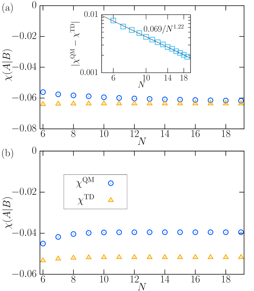
Figure 5: The same plots as in Fig. 4 of Sec. VII.3 for $\hat{A}=\hat{M}^{xx}$. In the inset of (a), the points can be fitted by a function $a/N^{b}$ with constants $a=0.069(2)$, $b=1.22(1)$, and the solid line shows the fitting function $0.069/N^{1.22}$.

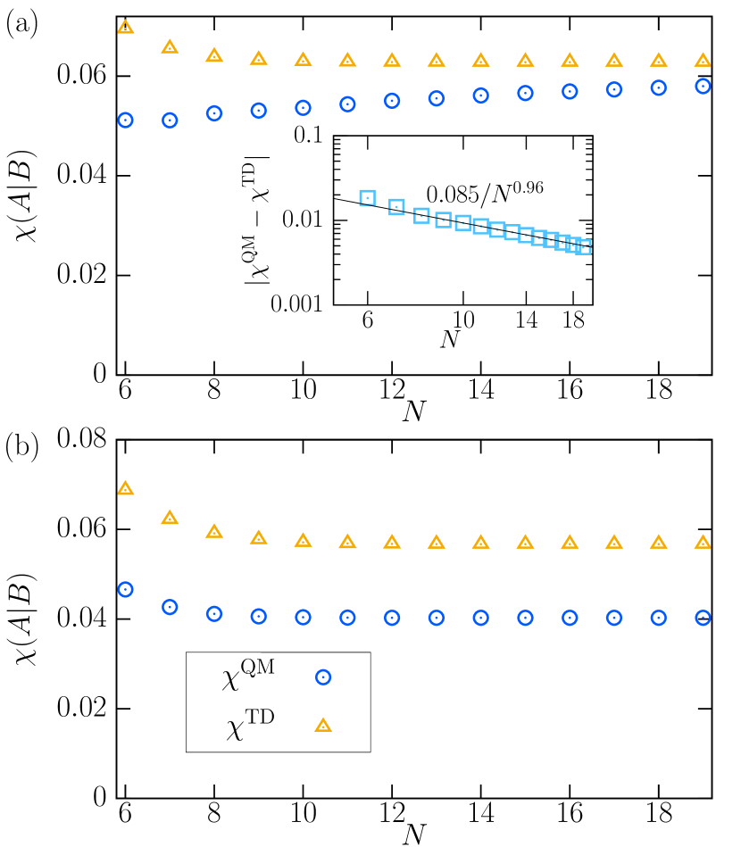
Figure 6: The same plots as in Fig. 4 of Sec. VII.3 for $\hat{A}=\hat{M}^{z1z}$. In the inset of (a), the points can be fitted by a function $a/N^{b}$ with constants $a=0.085(3)$, $b=0.96(1)$, and the solid line shows the fitting function $0.085/N^{0.96}$.

B.2 Susceptibilities of Model III

In this Appendix, we calculate the susceptibilities of Model III (see Table 1) in the same way as described in Sec. VII.1 or Appendix B.1.

First we investigate whether Model III satisfies condition (36). In Fig. 7, $\chi_{N}^{\text{QM}}(B|B)$ and $\chi_{N}^{\text{TD}}(B|B)$ of Model III are plotted against the system size $N$. This shows Model III violates condition (36). Hence, our Theorem (in the form rephrased in Sec. VI) indicates that some of the additive observables $\hat{A}$ do not satisfy Eq. (35). To investigate this point, we calculate, as in Sec. VII.3, $\chi^{\text{QM}}(A|B)$ and $\chi^{\text{TD}}(A|B)$ for three additive observables $\hat{A}=\hat{M}^{x},\hat{M}^{xx},\hat{M}^{z1z}$.

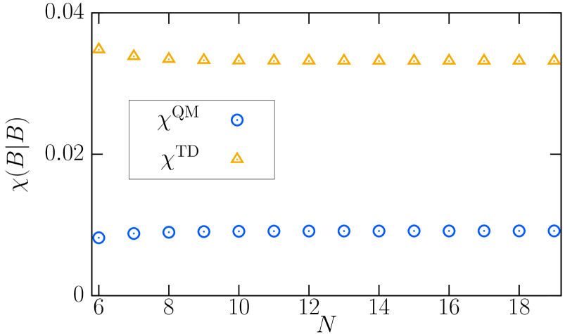
Figure 7: $\chi^{\text{QM}}_{N}(B|B)$ (blue circle) and $\chi^{\text{TD}}_{N}(B|B)$ (orange triangle) against the system size $N$ in an integrable system (Model III). The quench parameter is $f=J_{zz}$ and hence $\hat{B}=\hat{M}^{zz}$. This plot reveals that the condition (36) is violated in Model III.

In the main of Fig. 8, $\chi^{\text{QM}}_{N}(A|B)$ and $\chi^{\text{TD}}_{N}(A|B)$ are plotted against the system size $N$ for $\hat{A}=\hat{M}^{xx}$. It is seen that these susceptibilities deviate from each other, indicating the violation of Eq. (35).

The inset of Fig. 8 is the same plot for $\hat{A}=\hat{M}^{x}$. In this case, Eq. (35) is satisfied in the trivial form $\chi^{\text{QM}}_{N}(A|B)=\chi^{\text{TD}}_{N}(A|B)=0$, which follows from the spin rotation symmetry around $z$ axis. This does not contradict our Theorem, which does not state violation of Eq. (35) for all $\hat{A}$.

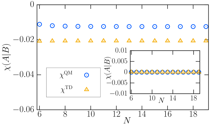
Figure 8: $\chi^{\text{QM}}_{N}(A|B)$ (blue circle) and $\chi^{\text{TD}}_{N}(A|B)$ (orange triangle) against the system size $N$ in an integrable system (Model III). The quench parameter is $f=J_{zz}$ and the observable of interest is $\hat{A}=\hat{M}^{xx}$. This plot reveals Eq. (35) is violated for $\hat{A}=\hat{M}^{xx}$ in Model III. Inset: The same plot as the main of this figure for $\hat{A}=\hat{M}^{x}$. The susceptibilities satisfy $\chi^{\text{QM}}_{N}(A|B)=\chi^{\text{TD}}_{N}(A|B)=0$ because of the spin rotation symmetry around $z$ axis.

Figure 9 shows the same plot as in Fig. 8 for $\hat{A}=\hat{M}^{z1z}$. Interestingly, $\chi^{\text{QM}}_{N}(A|B)$ and $\chi^{\text{TD}}_{N}(A|B)$ have opposite signs, which clearly indicates the violation of Eq. (35).

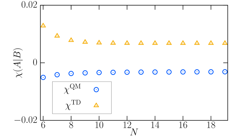
Figure 9: The same plots as in Fig. 8 for $\hat{A}=\hat{M}^{z1z}$. This plot reveals Eq. (35) is violated for $\hat{A}=\hat{M}^{z1z}$ in Model III.

B.3 Energy level spacings

In this Appendix, we study level spacing statistics of $\hat{H}_{0}$ for Models I, II and III, which are defined in Table 1.

Let $D_{k}$ be the dimension of the eigenspace of the lattice translation with an eigenvalue $e^{-ik}$ where $k=2\pi n_{k}/N$ ($n_{k}=0,1,...,N-1$) is wavenumber. We here label eigenvalues of $\hat{H}_{0}$ in this subspace using an integer $j=0,...,D_{k}-1$ as $E^{k}_{j}$, and sort them in ascending order, $E^{k}_{j}\leq E^{k}_{j+1}$ for all $j$. We consider the ratio of two consecutive energy level spacings $E^{k}_{j+1}-E^{k}_{j}$ and $E^{k}_{j+2}-E^{k}_{j+1}$ in the subspace

$$r^{k}_{j}:=\min\Bigl{\{}\frac{E^{k}_{j+2}-E^{k}_{j+1}}{E^{k}_{j+1}-E^{k}_{j}},\ \frac{E^{k}_{j+1}-E^{k}_{j}}{E^{k}_{j+2}-E^{k}_{j+1}}\Bigr{\}},$$ (125)

which satisfies $0\leq r^{k}_{j}\leq 1$. (When $E^{k}_{j+2}=E^{k}_{j+1}=E^{k}_{j}$, we define $r^{k}_{j}:=0$.) In order to investigate the level statistics in the bulk of energy spectrum, we use the ratios $r^{k}_{j}$ satisfying $D_{k}/4\leq j<3D_{k}/4$. By using all these ratios, we define the histogram of the ratio, $P_{k}(r)$. [We take the width of the interval of $r$ for the construction of $P_{k}(r)$ as $0.05$.]

Atas et al. [174] proposed the following functional forms of $P_{k}(r)$ using the random matrix theory. When the energy levels obey the Poisson law, $P_{k}(r)$ is given by

$$P_{\text{Poi}}(r):=2\frac{1}{(1+r)^{2}},$$ (126)

which is expected for typical integrable systems. When the energy levels obey the GUE, its $P_{k}(r)$ is well approximated by

$$P_{\text{GUE}}(r):=2\frac{81\sqrt{3}}{4\pi}\frac{(r+r^{2})^{2}}{(1+r+r^{2})^{4}}$$

$$\hskip 36.0pt+2\frac{0.578846}{(1+r)^{2}}\Bigl{\{}\Bigl{(}r+\frac{1}{r}\Bigr{)}^{-2}-4\frac{4-\pi}{3\pi-8}\Bigl{(}r+\frac{1}{r}\Bigr{)}^{-3}\Bigr{\}}.$$ (127)

This is expected for typical nonintegrable systems that have no symmetries other than the lattice translation. Furthermore, when the levels obey the Gaussian orthogonal ensemble (GOE), its $P_{k}(r)$ is well approximated by

$$P_{\text{GOE}}(r):=2\frac{27}{8}\frac{(r+r^{2})}{(1+r+r^{2})^{5/2}}$$

$$\hskip 36.0pt+2\frac{0.233378}{(1+r)^{2}}\Bigl{\{}\Bigl{(}r+\frac{1}{r}\Bigr{)}^{-1}-2\frac{\pi-2}{4-\pi}\Bigl{(}r+\frac{1}{r}\Bigr{)}^{-2}\Bigr{\}},$$ (128)

which is expected for typical nonintegrable systems.

We have numerically calculated $P_{k}(r)$ of our Models by the exact diagonalization, and compared the results with the above forms. Note that the symmetry properties of the subspace of wavenumber $k$ sometimes depend on whether $N$ is even or odd. In addition, the properties at special wavenumbers $k=0,\pi$ are sometimes very different from those at other wavenumbers. Therefore we consider three values of wavenumber $k=0,2\pi/N,\pi$ and both even and odd $N$. (Results for $k=\pi$ with odd $N$ are absent, since $k=\pi$ is impossible when $N$ is odd.)

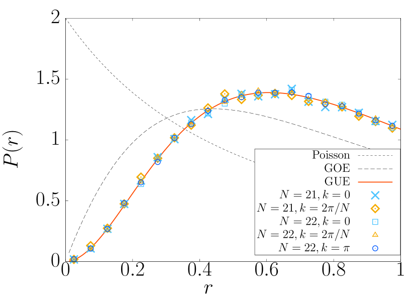
Figure 10: Histogram $P_{k}(r)$ of the ratio of consecutive energy level spacings of Model I in a momentum sector of wavenumber $k$. They are plotted for the system size $N=21,22$, and wavenumber $k=0,2\pi/N,\pi$. The solid line shows the GUE prediction $P_{\text{GUE}}(r)$, while two dashed lines show the distribution for the Poisson case $P_{\text{Poi}}(r)$ and the GOE prediction $P_{\text{GOE}}(r)$.

We plot $P_{k}(r)$ of Model I for $N=21,22$ in Fig. 10. It is well fitted by the GUE form $P_{\text{GUE}}(r)$ (solid line). For comparison, the Poisson form $P_{\text{Poi}}(r)$ and the GOE form $P_{\text{GOE}}(r)$ are depicted by the dashed lines, which clearly deviate from $P_{k}(r)$. These results indicate that Model I has no local conserved quantities other than the Hamiltonian.

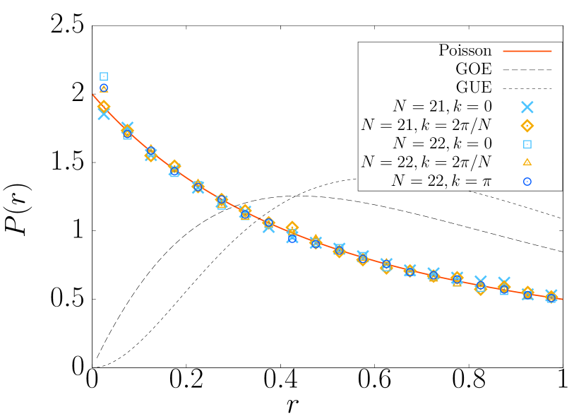
Figure 11: Same plot as in Fig. 10 for Model II. The solid line shows the distribution for the Poisson case $P_{\text{Poi}}(r)$, while two dashed lines show the GUE prediction $P_{\text{GUE}}(r)$ and the GOE prediction $P_{\text{GOE}}(r)$.

In Fig. 11, $P_{k}(r)$ of Model II is plotted for $N=21,22$. It is well fitted by the Poisson form $P_{\text{Poi}}(r)$ (solid line), while it clearly deviates from the GUE form $P_{\text{GUE}}(r)$ (dotted line) and the GOE form $P_{\text{GOE}}(r)$ (dashed line). These are consistent with the integrability of Model II.

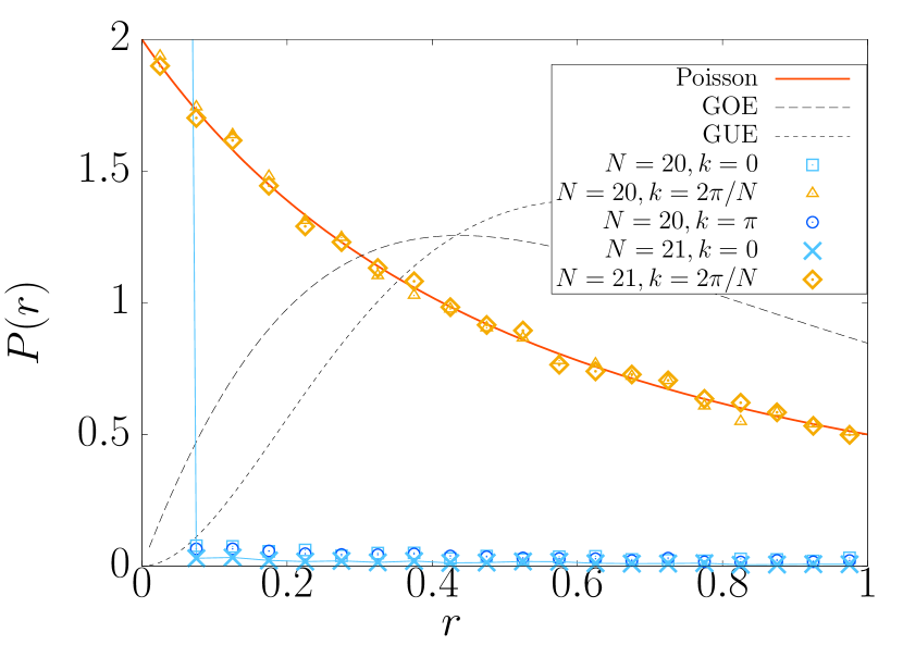
Figure 12: Same plot as in Fig. 10 for Model III. They are plotted for the system size $N=20,21$ and wavenumber $k=0,2\pi/N,\pi$. The orange solid line shows the distribution for the Poisson case $P_{\text{Poi}}(r)$, while two dashed lines show the GUE prediction $P_{\text{GUE}}(r)$ and the GOE prediction $P_{\text{GOE}}(r)$. The light blue solid line depicts the $\delta$ function like behavior of $P_{k}(r)$.

In Fig. 12, $P_{k}(r)$ of Model III is plotted for $N=20,21$. The $P_{k}(r)$ for $k=2\pi/N$ is well fitted by the Poisson form $P_{\text{Poi}}(r)$ (solid line). This is consistent with the integrability of Model III. On the other hand, $P_{k}(r)$ for $k=0,\pi$ show $\delta$-function-like behaviors, which are much different from the GUE form $P_{\text{GUE}}(r)$ (dotted line) and the GOE form $P_{\text{GOE}}(r)$ (dashed line). The $\delta$-function-like behaviors come from the fact that almost all energy eigenvalues have certain degeneracies . These degeneracies indicate that the subspaces of $k=0,\pi$ have additional non-Abelian symmetries, which would be related to the integrability of Model III .

Appendix C Analytic results for Model II

In this Appendix, we consider the following model

$$\hat{H} =-\sum_{r=1}^{N}\Bigl{(}J_{yy}\hat{\sigma}_{r}^{y}\hat{\sigma}_{r+1}^{y}+J_{zz}\hat{\sigma}_{r}^{z}\hat{\sigma}_{r+1}^{z}$$

$$\hskip 36.0pt+J_{yz}\hat{\sigma}_{r}^{y}\hat{\sigma}_{r+1}^{z}+J_{zy}\hat{\sigma}_{r}^{z}\hat{\sigma}_{r+1}^{y}+h_{x}\hat{\sigma}_{r}^{x}\Bigr{)},$$ (129)

which reduces to Model II by setting $J_{zy}=0$. This spin system can also be written as a fermionic system

$$\hat{H} =-\sum_{r=1}^{N-1}\Bigl{(}(J_{+-}\hat{c}_{r}^{\dagger}\hat{c}_{r+1}+\text{H.c.})+(J_{++}\hat{c}_{r}^{\dagger}\hat{c}_{r+1}^{\dagger}+\text{H.c.})$$

$$\hskip 36.0pt+h_{x}(2\hat{c}_{r}^{\dagger}\hat{c}_{r}-1)\Bigr{)}$$

$$\hskip 12.0pt+\hat{R}(J_{+-}\hat{c}_{N}^{\dagger}\hat{c}_{1}+\text{H.c.})+\hat{R}(J_{++}\hat{c}_{N}^{\dagger}\hat{c}_{1}^{\dagger}+\text{H.c.})$$

$$\hskip 12.0pt-h_{x}(2\hat{c}_{N}^{\dagger}\hat{c}_{N}-1),$$ (130)

by the Jordan-Wigner transformation

$$\hat{c}_{r}^{\dagger}=\frac{\hat{\sigma}_{r}^{y}+i\hat{\sigma}_{r}^{z}}{2}\prod_{r^{\prime}(<r)}(-\hat{\sigma}_{r^{\prime}}^{x}).$$ (131)

Here

$$\hat{R}:=\prod_{r=1}^{N}(-\hat{\sigma}_{r}^{x})=\prod_{r=1}^{N}(1-2\hat{c}_{r}^{\dagger}\hat{c}_{r})$$ (132)

and

$$J_{+-} :=J_{yy}+J_{zz}+iJ_{yz}-iJ_{zy},$$ (133)

$$J_{++} :=J_{yy}-J_{zz}-iJ_{yz}-iJ_{zy}.$$ (134)

The operator $\hat{R}$ takes $1$ for the states with even number of fermions, whereas it takes $-1$ for the states with odd number of fermions. Hence depending on whether the number of fermions is even or odd, terms containing $\hat{R}$ in Eq. (130) become the antiperiodic or periodic boundary condition, respectively.

To resolve this boundary condition that depends on $\hat{R}$, we consider two types of the Fourier transformation. We introduce two sets of wavenumbers

$$K^{\text{e}} :=\Bigl{\{}\frac{2\pi n_{k}}{N}+\frac{\pi}{N}\Bigm{|}n_{k}=0,1,...,N-1\Bigr{\}},$$ (135)

$$K^{\text{o}} :=\Bigl{\{}\frac{2\pi n_{k}}{N}\Bigm{|}n_{k}=0,1,...,N-1\Bigr{\}},$$ (136)

and perform the following Fourier transformation

$$\tilde{c}_{k}^{a}:=\sum_{r=1}^{N}\frac{e^{-ikr}}{\sqrt{N}}\hat{c}_{r}\qquad\text{for }k\in K^{a}\ (a=\text{e},\text{o}).$$ (137)

Using new fermionic operators, the Hamiltonian (130) can be written as

$$\hat{H} =-\sum_{a=\text{e},\text{o}}\hat{P}_{R}^{a}\sum_{k\in K^{a}}\Bigl{(}(J_{+-}e^{ik}\tilde{c}_{k}^{a\dagger}\tilde{c}_{k}^{a}+\text{H.c.})$$

$$\hskip 36.0pt+(J_{++}e^{ik}\tilde{c}_{k}^{a\dagger}\tilde{c}_{-k}^{a\dagger}+\text{H.c.})+h_{x}(2\tilde{c}_{k}^{a\dagger}\tilde{c}_{k}^{a}-1)\Bigr{)},$$ (138)

where

$$\hat{P}_{R}^{\text{e}} :=\frac{1+\hat{R}}{2},$$ (139)

$$\hat{P}_{R}^{\text{o}} :=\frac{1-\hat{R}}{2}$$ (140)

are the projection operators to the eigenspace of $\hat{R}$ with eigenvalues $1$ and $-1$, respectively.

When $J_{++}\neq 0$, Eq. (138) includes the off-diagonal terms $\tilde{c}_{k}^{a\dagger}\tilde{c}_{-k}^{a\dagger}$. To eliminate these, we perform the following Bogoliubov transformation for $k\neq 0,\pi$,

$$\hat{d}_{k}^{a}:=\cos\theta_{k}\tilde{c}_{k}^{a}+ie^{i\phi_{++}}\sin\theta_{k}\tilde{c}_{-k}^{a\dagger},$$ (141)

where $e^{i\phi_{++}}:=J_{++}/|J_{++}|$ and $\theta_{k}\in(-\pi/2,\pi/2)$ is determined from

$$\cos 2\theta_{k} =-\frac{2(\text{Re}[J_{+-}]\cos k+h_{x})}{r_{k}},$$ (142)

$$\sin 2\theta_{k} =-\frac{2|J_{++}|\sin k}{r_{k}}$$ (143)

with

$$r_{k}=2\sqrt{(\text{Re}[J_{+-}]\cos k+h_{x})^{2}+|J_{++}|^{2}\sin^{2}k}.$$ (144)

As a result, the Hamiltonian is given by

$$\hat{H} =-\sum_{a=\text{e},\text{o}}\hat{P}_{R}^{a}\sum_{k\in K^{a}\cap\{0,\pi\}}2(\text{Re}[J_{+-}]\cos k+h_{x})(\tilde{c}_{k}^{a\dagger}\tilde{c}_{k}^{a}-\frac{1}{2})$$

$$\hskip 12.0pt-\sum_{a=\text{e},\text{o}}\hat{P}_{R}^{a}\sum_{k\in K^{a}\setminus\{0,\pi\}}\varepsilon_{k}(\hat{d}_{k}^{a\dagger}\hat{d}_{k}^{a}-\frac{1}{2}),$$ (145)

where

$$\varepsilon_{k}:=r_{k}+2\text{Im}[J_{+-}]\sin k.$$ (146)

[Note that when $J_{++}=0$, Eq. (138) is already of the same form as the above.]

On the other hand, $\hat{B}$ given by Eq. (41) can be written as

$$\hat{B} =\sum_{a=\text{e},\text{o}}\hat{P}_{R}^{a}\sum_{k\in K^{a}}(\cos k\cos 2\theta_{k}+\sin k\sin 2\theta_{k}\cos\phi_{++})$$

$$\hskip 12.0pt\times(2\hat{d}_{k}^{a\dagger}\hat{d}_{k}^{a}-1)$$

$$\hskip 12.0pt+\sum_{a=\text{e},\text{o}}\hat{P}_{R}^{a}\sum_{k\in K^{a}}\Bigl{(}\bigl{(}-\cos k\,ie^{i\phi_{++}}\sin 2\theta_{k}$$

$$\hskip 36.0pt+i\sin k(\cos^{2}\theta_{k}-e^{2i\phi_{++}}\sin^{2}\theta_{k})\bigr{)}\hat{d}_{k}^{a\dagger}\hat{d}_{-k}^{a\dagger}+\text{H.c.}\Bigr{)}.$$ (147)

As a result, the susceptibilities of $\hat{B}$ can be calculated by using Eqs. (81) and (84) of Appendix A.1, whose thermodynamic limits are given by

$$\lim_{N\to\infty}\chi^{\text{QM}}_{N}(\hat{B}|\hat{B})$$

$$=\frac{1}{2\pi}\int_{0}^{2\pi}\differential{k}2\frac{e^{2\beta_{0}r_{k}}-1}{r_{k}}\frac{1}{e^{\beta_{0}\varepsilon_{k}}+1}\frac{1}{e^{\beta_{0}\varepsilon_{-k}}+1}$$

$$\hskip 5.0pt\times\bigl{|}-\cos k\,ie^{i\phi_{++}}\sin 2\theta_{k}+i\sin k(\cos^{2}\theta_{k}-e^{2i\phi_{++}}\sin^{2}\theta_{k})\bigr{|}^{2},$$ (148)

$$\lim_{N\to\infty}\chi^{\text{TD}}_{N}(\hat{B}|\hat{B})-\lim_{N\to\infty}\chi^{\text{QM}}_{N}(\hat{B}|\hat{B})$$

$$=\frac{\beta_{0}}{2\pi}\int_{0}^{2\pi}\differential{k}\frac{(\cos k\cos 2\theta_{k}+\sin k\sin 2\theta_{k}\cos\phi_{++}-C\varepsilon_{k})^{2}}{\cosh^{2}(\beta_{0}\varepsilon_{k}/2)},$$ (149)

where

$$C :=\frac{1}{2\pi}\int_{0}^{2\pi}\differential{k}\frac{\varepsilon_{k}(\cos k\cos 2\theta_{k}+\sin k\sin 2\theta_{k}\cos\phi_{++})}{\cosh^{2}(\beta_{0}\varepsilon_{k}/2)}$$

$$\hskip 12.0pt\Bigm{/}\frac{1}{2\pi}\int_{0}^{2\pi}\differential{k}\frac{\varepsilon_{k}^{2}}{\cosh^{2}(\beta_{0}\varepsilon_{k}/2)}.$$ (150)

References

- von Neumann [1929] J. von Neumann, Beweis des ergodensatzes und des H-theorems in der neuen mechanik, Z. Phys. 57, 30 (1929).
- Bocchieri and Loinger [1957] P. Bocchieri and A. Loinger, Quantum recurrence theorem, Physical Review 107, 337 (1957).
- Percival [1961] I. C. Percival, Almost periodicity and the quantal H theorem, Journal of Mathematical Physics 2, 235 (1961).
- Deutsch [1991] J. M. Deutsch, Quantum statistical mechanics in a closed system, Physical Review A 43, 2046 (1991).
- Srednicki [1994] M. Srednicki, Chaos and quantum thermalization, Physical Review E 50, 888 (1994).
- Tasaki [1998] H. Tasaki, From Quantum Dynamics to the Canonical Distribution: General Picture and a Rigorous Example, Physical Review Letters 80, 1373 (1998).
- Srednicki [1999] M. Srednicki, The approach to thermal equilibrium in quantized chaotic systems systems, Journal of Physics A : Mathematical and General 32, 1163 (1999).
- Goldstein et al. [2006] S. Goldstein, J. L. Lebowitz, R. Tumulka, and N. Zanghì, Canonical Typicality, Physical Review Letters 96, 050403 (2006).
- Popescu et al. [2006] S. Popescu, A. J. Short, and A. Winter, Entanglement and the foundations of statistical mechanics, Nature Physics 2, 754 (2006).
- Sugita [2006] A. Sugita, On the foundation of quantum statistical mechanics (in Japanese), RIMS Kokyuroku 1507, 147 (2006).
- Rigol et al. [2008] M. Rigol, V. Dunjko, and M. Olshanii, Thermalization and its mechanism for generic isolated quantum systems., Nature (London) 452, 854 (2008).
- Kim et al. [2014] H. Kim, T. N. Ikeda, and D. A. Huse, Testing whether all eigenstates obey the eigenstate thermalization hypothesis, Physical Review E - Statistical, Nonlinear, and Soft Matter Physics 90, 052105 (2014).
- Beugeling et al. [2014] W. Beugeling, R. Moessner, and M. Haque, Finite-size scaling of eigenstate thermalization, Physical Review E - Statistical, Nonlinear, and Soft Matter Physics 89, 042112 (2014).
- Steinigeweg et al. [2014] R. Steinigeweg, A. Khodja, H. Niemeyer, C. Gogolin, and J. Gemmer, Pushing the limits of the eigenstate thermalization hypothesis towards mesoscopic quantum systems, Physical Review Letters 112, 130403 (2014).
- Sirker et al. [2014] J. Sirker, N. P. Konstantinidis, F. Andraschko, and N. Sedlmayr, Locality and thermalization in closed quantum systems, Physical Review A - Atomic, Molecular, and Optical Physics 89, 042104 (2014).
- Mondaini et al. [2016] R. Mondaini, K. R. Fratus, M. Srednicki, and M. Rigol, Eigenstate thermalization in the two-dimensional transverse field Ising model, Physical Review E 93, 032104 (2016).
- Mondaini and Rigol [2017] R. Mondaini and M. Rigol, Eigenstate thermalization in the two-dimensional transverse field Ising model. II. Off-diagonal matrix elements of observables, Physical Review E 96, 012157 (2017).
- Bañuls et al. [2011] M. C. Bañuls, J. I. Cirac, and M. B. Hastings, Strong and Weak Thermalization of Infinite Nonintegrable Quantum Systems, Physical Review Letters 106, 050405 (2011).
- Goldstein et al. [2015] S. Goldstein, D. A. Huse, J. L. Lebowitz, and R. Tumulka, Thermal Equilibrium of a Macroscopic Quantum System in a Pure State, Physical Review Letters 115, 100402 (2015).
- Tasaki [2016] H. Tasaki, Journal of Statistical Physics, Vol. 163 (Springer US, New York, 2016) pp. 937–997.
- Goldstein et al. [2017] S. Goldstein, D. A. Huse, J. L. Lebowitz, and R. Tumulka, Macroscopic and microscopic thermal equilibrium, Annalen der Physik 529, 1600301 (2017).
- De Palma et al. [2015] G. De Palma, A. Serafini, V. Giovannetti, and M. Cramer, Necessity of Eigenstate Thermalization, Physical Review Letters 115, 220401 (2015).
- Reimann [2015] P. Reimann, Generalization of von Neumann’s Approach to Thermalization, Physical Review Letters 115, 010403 (2015).
- Shiraishi and Mori [2017] N. Shiraishi and T. Mori, Systematic Construction of Counterexamples to the Eigenstate Thermalization Hypothesis, Physical Review Letters 119, 030601 (2017).
- Mori and Shiraishi [2017] T. Mori and N. Shiraishi, Thermalization without eigenstate thermalization hypothesis after a quantum quench, Physical Review E 96, 022153 (2017).
- Hamazaki and Ueda [2018] R. Hamazaki and M. Ueda, Atypicality of Most Few-Body Observables, Physical Review Letters 120, 080603 (2018).
- Lashkari et al. [2018] N. Lashkari, A. Dymarsky, and H. Liu, Eigenstate thermalization hypothesis in conformal field theory, Journal of Statistical Mechanics: Theory and Experiment 2018, 033101 (2018).
- Anza et al. [2018] F. Anza, C. Gogolin, and M. Huber, Eigenstate Thermalization for Degenerate Observables, Physical Review Letters 120, 150603 (2018).
- Brenes et al. [2020] M. Brenes, T. Leblond, J. Goold, and M. Rigol, Eigenstate Thermalization in a Locally Perturbed Integrable System, Physical Review Letters 125, 70605 (2020).
- Sugimoto et al. [2021] S. Sugimoto, R. Hamazaki, and M. Ueda, Test of the Eigenstate Thermalization Hypothesis Based on Local Random Matrix Theory, Physical Review Letters 126, 120602 (2021).
- Dymarsky [2022] A. Dymarsky, Bound on Eigenstate Thermalization from Transport, Physical Review Letters 128, 190601 (2022).
- Sugimoto et al. [2022] S. Sugimoto, R. Hamazaki, and M. Ueda, Eigenstate Thermalization in Long-Range Interacting Systems, Physical Review Letters 129, 30602 (2022).
- Wang et al. [2022] Q. Q. Wang, S. J. Tao, W. W. Pan, Z. Chen, G. Chen, K. Sun, J. S. Xu, X. Y. Xu, Y. J. Han, C. F. Li, and G. C. Guo, Experimental verification of generalized eigenstate thermalization hypothesis in an integrable system, Light: Sci. Appl. 11, 194 (2022).
- Biroli et al. [2010] G. Biroli, C. Kollath, and A. M. Läuchli, Effect of Rare Fluctuations on the Thermalization of Isolated Quantum Systems, Physical Review Letters 105, 250401 (2010).
- Ikeda et al. [2013] T. N. Ikeda, Y. Watanabe, and M. Ueda, Finite-size scaling analysis of the eigenstate thermalization hypothesis in a one-dimensional interacting Bose gas, Physical Review E - Statistical, Nonlinear, and Soft Matter Physics 87, 012125 (2013).
- Alba [2015] V. Alba, Eigenstate thermalization hypothesis and integrability in quantum spin chains, Physical Review B - Condensed Matter and Materials Physics 91, 155123 (2015).
- [37] T. Mori, Weak eigenstate thermalization with large deviation bound, arXiv:1609.09776 .
- Iyoda et al. [2017] E. Iyoda, K. Kaneko, and T. Sagawa, Fluctuation Theorem for Many-Body Pure Quantum States, Physical Review Letters 119, 100601 (2017).
- Kinoshita et al. [2006] T. Kinoshita, T. Wenger, and D. S. Weiss, A quantum Newton’s cradle, Nature (London) 440, 900 (2006).
- Hofferberth et al. [2007] S. Hofferberth, I. Lesanovsky, B. Fischer, T. Schumm, and J. Schmiedmayer, Non-equilibrium coherence dynamics in one-dimensional Bose gases, Nature (London) 449, 324 (2007).
- Gring et al. [2012] M. Gring, M. Kuhnert, T. Langen, T. Kitagawa, B. Rauer, M. Schreitl, I. Mazets, D. A. Smith, E. Demler, and J. Schmiedmayer, Relaxation and Prethermalization in an Isolated Quantum System, Science 337, 1318 (2012).
- Trotzky et al. [2012] S. Trotzky, Y. A. Chen, A. Flesch, I. P. McCulloch, U. Schollwöck, J. Eisert, and I. Bloch, Probing the relaxation towards equilibrium in an isolated strongly correlated one-dimensional Bose gas, Nature Physics 8, 325 (2012).
- Adu Smith et al. [2013] D. Adu Smith, M. Gring, T. Langen, M. Kuhnert, B. Rauer, R. Geiger, T. Kitagawa, I. Mazets, E. Demler, and J. Schmiedmayer, Prethermalization revealed by the relaxation dynamics of full distribution functions, New Journal of Physics 15, 075011 (2013).
- Langen et al. [2015] T. Langen, S. Erne, R. Geiger, B. Rauer, T. Schweigler, M. Kuhnert, W. Rohringer, I. E. Mazets, T. Gasenzer, and J. Schmiedmayer, Experimental observation of a generalized Gibbs ensemble, Science 348, 207 (2015).
- Kaufman et al. [2016] A. M. Kaufman, M. E. Tai, A. Lukin, M. Rispoli, R. Schittko, P. M. Preiss, and M. Greiner, Quantum thermalization through entanglement in an isolated many-body system, Science 353, 794 (2016).
- Bernien et al. [2017] H. Bernien, S. Schwartz, A. Keesling, H. Levine, A. Omran, H. Pichler, S. Choi, A. S. Zibrov, M. Endres, M. Greiner, V. Vuletic, and M. D. Lukin, Probing many-body dynamics on a 51-atom quantum simulator, Nature (London) 551, 579 (2017).
- Orioli et al. [2018] A. P. Orioli, A. Signoles, H. Wildhagen, G. Günter, J. Berges, S. Whitlock, and M. Weidemüller, Relaxation of an Isolated Dipolar-Interacting Rydberg Quantum Spin System, Physical Review Letters 120, 63601 (2018).
- Tang et al. [2018] Y. Tang, W. Kao, K. Y. Li, S. Seo, K. Mallayya, M. Rigol, S. Gopalakrishnan, and B. L. Lev, Thermalization near Integrability in a Dipolar Quantum Newton’s Cradle, Physical Review X 8, 21030 (2018).
- Richerme et al. [2014] P. Richerme, Z. X. Gong, A. Lee, C. Senko, J. Smith, M. Foss-Feig, S. Michalakis, A. V. Gorshkov, and C. Monroe, Non-local propagation of correlations in quantum systems with long-range interactions, Nature (London) 511, 198 (2014).
- Clos et al. [2016] G. Clos, D. Porras, U. Warring, and T. Schaetz, Time-Resolved Observation of Thermalization in an Isolated Quantum System, Physical Review Letters 117, 170401 (2016).
- Smith et al. [2016] J. Smith, A. Lee, P. Richerme, B. Neyenhuis, P. W. Hess, P. Hauke, M. Heyl, D. A. Huse, and C. Monroe, Many-body localization in a quantum simulator with programmable random disorder, Nature Physics 12, 907 (2016).
- Hess et al. [2017] P. W. Hess, P. Becker, H. B. Kaplan, A. Kyprianidis, A. C. Lee, B. Neyenhuis, G. Pagano, P. Richerme, C. Senko, J. Smith, W. L. Tan, J. Zhang, and C. Monroe, Non-thermalization in trapped atomic ion spin chains, Philosophical Transactions of the Royal Society A: Mathematical, Physical and Engineering Sciences 375, 20170107 (2017).
- Neill et al. [2016] C. Neill, P. Roushan, M. Fang, Y. Chen, M. Kolodrubetz, Z. Chen, A. Megrant, R. Barends, B. Campbell, B. Chiaro, A. Dunsworth, E. Jeffrey, J. Kelly, J. Mutus, P. J. O’Malley, C. Quintana, D. Sank, A. Vainsencher, J. Wenner, T. C. White, A. Polkovnikov, and J. M. Martinis, Ergodic dynamics and thermalization in an isolated quantum system, Nature Physics 12, 1037 (2016).
- Xu et al. [2018] K. Xu, J. J. Chen, Y. Zeng, Y. R. Zhang, C. Song, W. Liu, Q. Guo, P. Zhang, D. Xu, H. Deng, K. Huang, H. Wang, X. Zhu, D. Zheng, and H. Fan, Emulating Many-Body Localization with a Superconducting Quantum Processor, Physical Review Letters 120, 050507 (2018).
- Guo et al. [2021] Q. Guo, C. Cheng, Z. H. Sun, Z. Song, H. Li, Z. Wang, W. Ren, H. Dong, D. Zheng, Y. R. Zhang, R. Mondaini, H. Fan, and H. Wang, Observation of energy-resolved many-body localization, Nature Physics 17, 234 (2021).
- Chen et al. [2021] F. Chen, Z. H. Sun, M. Gong, Q. Zhu, Y. R. Zhang, Y. Wu, Y. Ye, C. Zha, S. Li, S. Guo, H. Qian, H. L. Huang, J. Yu, H. Deng, H. Rong, J. Lin, Y. Xu, L. Sun, C. Guo, N. Li, F. Liang, C. Z. Peng, H. Fan, X. Zhu, and J. W. Pan, Observation of Strong and Weak Thermalization in a Superconducting Quantum Processor, Physical Review Letters 127, 25 (2021).
- Darkwah Oppong et al. [2022] N. Darkwah Oppong, G. Pasqualetti, O. Bettermann, P. Zechmann, M. Knap, I. Bloch, and S. Fölling, Probing Transport and Slow Relaxation in the Mass-Imbalanced Fermi-Hubbard Model, Physical Review X 12, 031026 (2022).
- Abuzarli et al. [2022] M. Abuzarli, N. Cherroret, T. Bienaimé, and Q. Glorieux, Nonequilibrium Prethermal States in a Two-Dimensional Photon Fluid, Physical Review Letters 129, 100602 (2022).
- D’Alessio et al. [2016] L. D’Alessio, Y. Kafri, A. Polkovnikov, and M. Rigol, From quantum chaos and eigenstate thermalization to statistical mechanics and thermodynamics, Advances in Physics 65, 239 (2016).
- Gogolin and Eisert [2016] C. Gogolin and J. Eisert, Equilibration, thermalisation, and the emergence of statistical mechanics in closed quantum systems, Reports on Progress in Physics 79, 056001 (2016).
- Mori et al. [2018] T. Mori, T. N. Ikeda, E. Kaminishi, and M. Ueda, Thermalization and prethermalization in isolated quantum systems: A theoretical overview, Journal of Physics B: Atomic, Molecular and Optical Physics 51, 112001 (2018).
- Bohrdt et al. [2017] A. Bohrdt, C. B. Mendl, M. Endres, and M. Knap, Scrambling and thermalization in a diffusive quantum many-body system, New Journal of Physics 19, 063001 (2017).
- Schnaack et al. [2019] O. Schnaack, N. Bölter, S. Paeckel, S. R. Manmana, S. Kehrein, and M. Schmitt, Tripartite information, scrambling, and the role of Hilbert space partitioning in quantum lattice models, Physical Review B 100, 224302 (2019).
- Zhu et al. [2022] Q. Zhu, Z. H. Sun, M. Gong, F. Chen, Y. R. Zhang, Y. Wu, Y. Ye, C. Zha, S. Li, S. Guo, H. Qian, H. L. Huang, J. Yu, H. Deng, H. Rong, J. Lin, Y. Xu, L. Sun, C. Guo, N. Li, F. Liang, C. Z. Peng, H. Fan, X. Zhu, and J. W. Pan, Observation of Thermalization and Information Scrambling in a Superconducting Quantum Processor, Physical Review Letters 128, 160502 (2022).
- Hayden and Preskill [2007] P. Hayden and J. Preskill, Black holes as mirrors: Quantum information in random subsystems, Journal of High Energy Physics 2007, 120 (2007).
- Sekino and Susskind [2008] Y. Sekino and L. Susskind, Fast scramblers, Journal of High Energy Physics 2008, 065 (2008).
- Shenker and Stanford [2014a] S. H. Shenker and D. Stanford, Black holes and the butterfly effect, Journal of High Energy Physics 2014, 067 (2014a).
- Shenker and Stanford [2014b] S. H. Shenker and D. Stanford, Multiple shocks, Journal of High Energy Physics 2014, 46 (2014b).
- Shenker and Stanford [2015] S. H. Shenker and D. Stanford, Stringy effects in scrambling, Journal of High Energy Physics 2015, 132 (2015).
- Roberts et al. [2015] D. A. Roberts, D. Stanford, and L. Susskind, Localized shocks, Journal of High Energy Physics 2015, 51 (2015).
- Roberts and Stanford [2015] D. A. Roberts and D. Stanford, Diagnosing Chaos Using Four-Point Functions in Two-Dimensional Conformal Field Theory, Physical Review Letters 115, 131603 (2015).
- Hosur et al. [2016] P. Hosur, X. L. Qi, D. A. Roberts, and B. Yoshida, Chaos in quantum channels, Journal of High Energy Physics 2016, 004 (2016).
- Balachandran et al. [2021] V. Balachandran, G. Benenti, G. Casati, and D. Poletti, From the eigenstate thermalization hypothesis to algebraic relaxation of OTOCs in systems with conserved quantities, Physical Review B 104, 104306 (2021).
- Brenes et al. [2021] M. Brenes, S. Pappalardi, M. T. Mitchison, J. Goold, and A. Silva, Out-of-time-order correlations and the fine structure of eigenstate thermalization, Physical Review E 104, 034120 (2021).
- Rigol et al. [2007] M. Rigol, V. Dunjko, V. Yurovsky, and M. Olshanii, Relaxation in a Completely Integrable Many-Body Quantum System: An Ab initio Study of the Dynamics of the Highly Excited States of 1D Lattice Hard-Core Bosons, Physical Review Letters 98, 050405 (2007).
- Fagotti [2014] M. Fagotti, On conservation laws, relaxation and pre-relaxation after a quantum quench, Journal of Statistical Mechanics: Theory and Experiment 2014, P03016 (2014).
- Vidmar and Rigol [2016] L. Vidmar and M. Rigol, Generalized Gibbs ensemble in integrable lattice models, Journal of Statistical Mechanics: Theory and Experiment 2016, 064007 (2016).
- Pozsgay et al. [2014] B. Pozsgay, M. Mestyán, M. A. Werner, M. Kormos, G. Zaránd, and G. Takács, Correlations after quantum quenches in the XXZ Spin Chain: Failure of the generalized Gibbs ensemble, Physical Review Letters 113, 117203 (2014).
- Wouters et al. [2014] B. Wouters, J. De Nardis, M. Brockmann, D. Fioretto, M. Rigol, and J. S. Caux, Quenching the anisotropic Heisenberg chain: Exact solution and generalized gibbs ensemble predictions, Physical Review Letters 113, 117202 (2014).
- Mierzejewski et al. [2015] M. Mierzejewski, P. Prelovšek, and T. Prosen, Identifying Local and Quasilocal Conserved Quantities in Integrable Systems, Physical Review Letters 114, 140601 (2015).
- Ilievski et al. [2015a] E. Ilievski, M. Medenjak, and T. Prosen, Quasilocal Conserved Operators in the Isotropic Heisenberg Spin- 1/2 Chain, Physical Review Letters 115, 120601 (2015a).
- Ilievski et al. [2015b] E. Ilievski, J. De Nardis, B. Wouters, J. S. Caux, F. H. Essler, and T. Prosen, Complete Generalized Gibbs Ensembles in an Interacting Theory, Physical Review Letters 115, 157201 (2015b).
- Doyon [2017] B. Doyon, Thermalization and Pseudolocality in Extended Quantum Systems, Communications in Mathematical Physics 351, 155 (2017).
- Mitsuhashi et al. [2022] Y. Mitsuhashi, K. Kaneko, and T. Sagawa, Characterizing Symmetry-Protected Thermal Equilibrium by Work Extraction, Physical Review X 12, 21013 (2022).
- Bertini et al. [2022] B. Bertini, F. H. Essler, and E. Granet, Bogoliubov-Born-Green-Kirkwood-Yvon Hierarchy and Generalized Hydrodynamics, Physical Review Letters 128, 190401 (2022).
- Yang and Del Campo [2022] J. Yang and A. Del Campo, One-Dimensional Quantum Systems with Ground State of Jastrow Form Are Integrable, Physical Review Letters 129, 150601 (2022).
- Cataldini et al. [2022] F. Cataldini, F. Møller, M. Tajik, J. Sabino, S. C. Ji, I. Mazets, T. Schweigler, B. Rauer, and J. Schmiedmayer, Emergent Pauli Blocking in a Weakly Interacting Bose Gas, Physical Review X 12, 41032 (2022).
- Oganesyan and Huse [2007] V. Oganesyan and D. A. Huse, Localization of interacting fermions at high temperature, Physical Review B - Condensed Matter and Materials Physics 75, 155111 (2007).
- Pal and Huse [2010] A. Pal and D. A. Huse, Many-body localization phase transition, Physical Review B - Condensed Matter and Materials Physics 82, 174411 (2010).
- Imbrie [2016] J. Z. Imbrie, On many-body localization for quantum spin chains, Journal of Statistical Physics 163, 998 (2016).
- Roy et al. [2020] N. Roy, A. Ramachandran, and A. Sharma, Interplay of disorder and interactions in a flat-band supporting diamond chain, Physical Review Research 2, 043395 (2020).
- Danieli et al. [2020] C. Danieli, A. Andreanov, and S. Flach, Many-body flatband localization, Physical Review B 102, 041116 (2020).
- McClarty et al. [2020] P. A. McClarty, M. Haque, A. Sen, and J. Richter, Disorder-free localization and many-body quantum scars from magnetic frustration, Physical Review B 102, 224303 (2020).
- Kuno et al. [2020] Y. Kuno, T. Orito, and I. Ichinose, Flat-band many-body localization and ergodicity breaking in the Creutz ladder, New Journal of Physics 22, 013032 (2020).
- [95] M. Daumann, R. Steinigeweg, and T. Dahm, Many-Body Localization in Translational Invariant Diamond Ladders with Flat Bands, arXiv:2009.09705 .
- Vu et al. [2022] D. D. Vu, K. Huang, X. Li, and S. Das Sarma, Fermionic Many-Body Localization for Random and Quasiperiodic Systems in the Presence of Short-and Long-Range Interactions, Physical Review Letters 128, 146601 (2022).
- Balducci et al. [2022] F. Balducci, A. Gambassi, A. Lerose, A. Scardicchio, and C. Vanoni, Localization and Melting of Interfaces in the Two-Dimensional Quantum Ising Model, Physical Review Letters 129, 120601 (2022).
- Krajewski et al. [2022] B. Krajewski, L. Vidmar, J. Bonča, and M. Mierzejewski, Restoring Ergodicity in a Strongly Disordered Interacting Chain, Physical Review Letters 129, 260601 (2022).
- Schreiber et al. [2015] M. Schreiber, S. S. Hodgman, P. Bordia, H. P. Lüschen, M. H. Fischer, R. Vosk, E. Altman, U. Schneider, and I. Bloch, Observation of many-body localization of interacting fermions in a quasirandom optical lattice, Science 349, 842 (2015).
- Kondov et al. [2015] S. S. Kondov, W. R. McGehee, W. Xu, and B. Demarco, Disorder-Induced Localization in a Strongly Correlated Atomic Hubbard Gas, Physical Review Letters 114, 083002 (2015).
- Choi et al. [2016] J.-y. Choi, S. Hild, J. Zeiher, P. Schauß, A. Rubio-Abadal, T. Yefsah, V. Khemani, D. A. Huse, I. Bloch, and C. Gross, Exploring the many-body localization transition in two dimensions, Science 352, 1547 (2016).
- Wei et al. [2018] K. X. Wei, C. Ramanathan, and P. Cappellaro, Exploring Localization in Nuclear Spin Chains, Physical Review Letters 120, 70501 (2018).
- Nandkishore and Huse [2015] R. Nandkishore and D. A. Huse, Many-body localization and thermalization in quantum statistical mechanics, Annual Review of Condensed Matter Physics 6, 15 (2015).
- Altman and Vosk [2015] E. Altman and R. Vosk, Universal dynamics and renormalization in many-body-localized systems, Annual Review of Condensed Matter Physics 6, 383 (2015).
- Abanin et al. [2019] D. A. Abanin, E. Altman, I. Bloch, and M. Serbyn, Colloquium: Many-body localization, thermalization, and entanglement, Reviews of Modern Physics 91, 21001 (2019).
- Heller [1984] E. J. Heller, Bound-State Eigenfunctions of Classically Chaotic Hamiltonian Systems: Scars of Periodic Orbits, Physical Review Letters 53, 1515 (1984).
- Turner et al. [2018a] C. J. Turner, A. A. Michailidis, D. A. Abanin, M. Serbyn, and Z. Papić, Weak ergodicity breaking from quantum many-body scars, Nature Physics 14, 745 (2018a).
- Turner et al. [2018b] C. J. Turner, A. A. Michailidis, D. A. Abanin, M. Serbyn, and Z. Papić, Quantum scarred eigenstates in a Rydberg atom chain: Entanglement, breakdown of thermalization, and stability to perturbations, Physical Review B 94, 155134 (2018b).
- Moudgalya et al. [2018a] S. Moudgalya, S. Rachel, B. A. Bernevig, and N. Regnault, Exact excited states of nonintegrable models, Physical Review B 98, 235155 (2018a).
- Moudgalya et al. [2018b] S. Moudgalya, N. Regnault, and B. A. Bernevig, Entanglement of exact excited states of Affleck-Kennedy-Lieb-Tasaki models: Exact results, many-body scars, and violation of the strong eigenstate thermalization hypothesis, Physical Review B 98, 235156 (2018b).
- Alhambra et al. [2020a] Á. M. Alhambra, A. Anshu, and H. Wilming, Revivals imply quantum many-body scars, Physical Review B 101, 205107 (2020a).
- Moudgalya et al. [2020] S. Moudgalya, N. Regnault, and B. A. Bernevig, -pairing in Hubbard models: From spectrum generating algebras to quantum many-body scars, Physical Review B 102, 085140 (2020).
- Bull et al. [2020] K. Bull, J. Y. Desaules, and Z. Papić, Quantum scars as embeddings of weakly broken Lie algebra representations, Physical Review B 101, 165139 (2020).
- Windt and Pichler [2022] B. Windt and H. Pichler, Squeezing Quantum Many-Body Scars, Physical Review Letters 128, 90606 (2022).
- Desaules et al. [2022] J. Y. Desaules, F. Pietracaprina, Z. Papić, J. Goold, and S. Pappalardi, Extensive Multipartite Entanglement from SU(2) Quantum Many-Body Scars, Physical Review Letters 129, 020601 (2022).
- Huang et al. [2022] B. Huang, T. H. Leung, D. M. Stamper-Kurn, and W. V. Liu, Discrete Time Crystals Enforced by Floquet-Bloch Scars, Physical Review Letters 129, 133001 (2022).
- Bull et al. [2022] K. Bull, A. Hallam, Z. Papić, and I. Martin, Tuning between Continuous Time Crystals and Many-Body Scars in Long-Range XYZ Spin Chains, Physical Review Letters 129, 140602 (2022).
- De Tomasi et al. [2019] G. De Tomasi, D. Hetterich, P. Sala, and F. Pollmann, Dynamics of strongly interacting systems: From Fock-space fragmentation to many-body localization, Physical Review B 100, 214313 (2019).
- Moudgalya et al. [2021] S. Moudgalya, A. Prem, N. Regnault, R. Nandkishore, and B. A. Bernevig, Thermalization and Its Absence within Krylov Subspaces of a Constrained Hamiltonian, in Memorial Volume for Shoucheng Zhang (World Scientific, Singapole, 2021) Chap. 7, pp. 147–209.
- Buča [2022] B. Buča, Out-of-Time-Ordered Crystals and Fragmentation, Physical Review Letters 128, 100601 (2022).
- Moudgalya and Motrunich [2022] S. Moudgalya and O. I. Motrunich, Hilbert Space Fragmentation and Commutant Algebras, Physical Review X 12, 11050 (2022).
- Bastianello et al. [2022] A. Bastianello, U. Borla, and S. Moroz, Fragmentation and Emergent Integrable Transport in the Weakly Tilted Ising Chain, Physical Review Letters 128, 196601 (2022).
- Yoshinaga et al. [2022] A. Yoshinaga, H. Hakoshima, T. Imoto, Y. Matsuzaki, and R. Hamazaki, Emergence of Hilbert Space Fragmentation in Ising Models with a Weak Transverse Field, Physical Review Letters 129, 90602 (2022).
- Kohlert et al. [2023] T. Kohlert, S. Scherg, P. Sala, F. Pollmann, B. Hebbe Madhusudhana, I. Bloch, and M. Aidelsburger, Exploring the Regime of Fragmentation in Strongly Tilted Fermi-Hubbard Chains, Physical Review Letters 130, 10201 (2023).
- LeBlond et al. [2019] T. LeBlond, K. Mallayya, L. Vidmar, and M. Rigol, Entanglement and matrix elements of observables in interacting integrable systems, Physical Review E 100, 062134 (2019).
- Bauer and Nayak [2013] B. Bauer and C. Nayak, Area laws in a many-body localized state and its implications for topological order, Journal of Statistical Mechanics: Theory and Experiment 2013, P09005 (2013).
- Garrison and Grover [2018] J. R. Garrison and T. Grover, Does a Single Eigenstate Encode the Full Hamiltonian?, Physical Review X 8, 21026 (2018).
- Ippoliti et al. [2022] M. Ippoliti, T. Rakovszky, and V. Khemani, Fractal, Logarithmic, and Volume-Law Entangled Nonthermal Steady States via Spacetime Duality, Physical Review X 12, 11045 (2022).
- Mueller et al. [2022] N. Mueller, T. V. Zache, and R. Ott, Thermalization of Gauge Theories from their Entanglement Spectrum, Physical Review Letters 129, 11601 (2022).
- Comparin et al. [2022] T. Comparin, F. Mezzacapo, and T. Roscilde, Multipartite Entangled States in Dipolar Quantum Simulators, Physical Review Letters 129, 150503 (2022).
- Kollath et al. [2007] C. Kollath, A. M. Läuchli, and E. Altman, Quench Dynamics and Nonequilibrium Phase Diagram of the Bose-Hubbard Model, Physical Review Letters 98, 180601 (2007).
- Rigol [2009a] M. Rigol, Breakdown of Thermalization in Finite One-Dimensional Systems, Physical Review Letters 103, 100403 (2009a).
- Rigol [2009b] M. Rigol, Quantum quenches and thermalization in one-dimensional fermionic systems, Physical Review A - Atomic, Molecular, and Optical Physics 80, 053607 (2009b).
- Zill et al. [2015] J. C. Zill, T. M. Wright, K. V. Kheruntsyan, T. Gasenzer, and M. J. Davis, Relaxation dynamics of the Lieb-Liniger gas following an interaction quench: A coordinate Bethe-ansatz analysis, Physical Review A - Atomic, Molecular, and Optical Physics 91, 023611 (2015).
- Chiba et al. [2020] Y. Chiba, K. Asano, and A. Shimizu, Anomalous Behavior of Magnetic Susceptibility Obtained by Quench Experiments in Isolated Quantum Systems, Physical Review Letters 124, 110609 (2020).
- Kubo [1957] R. Kubo, Statistical-mechanical theory of irreversible processes. I. General theory and simple applications to magnetic and conduction problems, Journal of the Physical Society of Japan 12, 570 (1957).
- Wilcox [1968] R. M. Wilcox, Bounds for the isothermal, adiabatic, and isolated static susceptibility tensors, Physical Review 174, 624 (1968).
- Mazur [1969] P. Mazur, Non-ergodicity of phase functions in certain systems, Physica 43, 533 (1969).
- Suzuki [1971] M. Suzuki, Ergodicity, constants of motion, and bounds for susceptibilities, Physica 51, 277 (1971).
- Landau and Lifshitz [1980] L. D. Landau and E. M. Lifshitz, Statistical Physics, 3rd ed. (Butterworth-Heinemann, Oxford, 1980) p. 544.
- Oono [2017] Y. Oono, Perspectives on Statistical Thermodynamics (Cambridge University Press, Cambridge, 2017).
- Shimizu [2021] A. Shimizu, Netsurikigaku No Kiso [Principles of Thermodynamics], 2nd ed. (University of Tokyo Press, Tokyo, 2021).
- Note [1] For boson systems, the Hilbert space can be made finite dimensional by fixing the total particle number or by introducing an appropriate cutoff.
- Note [2] We assume that all matrix elements of are twice differentiable.
- Note [3] If one lifted this basic assumption of thermodynamics [221, 222], as in the generalized Gibbs ensemble, almost all systems including integrable systems would satisfy Criterion (i) given in Sec. III [15, 83].
- Short and Farrelly [2012] A. J. Short and T. C. Farrelly, Quantum equilibration in finite time, New Journal of Physics 14, 013063 (2012).
- Srednicki [1996] M. Srednicki, Thermal fluctuations in quantized chaotic systems, Journal of Physics A: Mathematical and General 29, L75 (1996).
- Khodja et al. [2015] A. Khodja, R. Steinigeweg, and J. Gemmer, Relevance of the eigenstate thermalization hypothesis for thermal relaxation, Physical Review E - Statistical, Nonlinear, and Soft Matter Physics 91, 012120 (2015).
- Reimann [2008] P. Reimann, Foundation of Statistical Mechanics under Experimentally Realistic Conditions, Physical Review Letters 101, 1190403 (2008).
- Linden et al. [2009] N. Linden, S. Popescu, A. J. Short, and A. Winter, Quantum mechanical evolution towards thermal equilibrium, Physical Review E - Statistical, Nonlinear, and Soft Matter Physics 79, 061103 (2009).
- Note [4] The order of three limits (regarding , and ) in Eq. (26) should be understood as in Eq. (24).
- Berges et al. [2004] J. Berges, S. Borsányi, and C. Wetterich, Prethermalization, Physical Review Letters 93, 142002 (2004).
- Moeckel and Kehrein [2008] M. Moeckel and S. Kehrein, Interaction Quench in the Hubbard Model, Physical Review Letters 100, 175702 (2008).
- Moeckel and Kehrein [2009] M. Moeckel and S. Kehrein, Real-time evolution for weak interaction quenches in quantum systems, Annals of Physics 324, 2146 (2009).
- Moeckel and Kehrein [2010] M. Moeckel and S. Kehrein, Crossover from adiabatic to sudden interaction quenches in the Hubbard model: Prethermalization and non-equilibrium dynamics, New Journal of Physics 12, 055016 (2010).
- Kollar et al. [2011] M. Kollar, F. A. Wolf, and M. Eckstein, Generalized Gibbs ensemble prediction of prethermalization plateaus and their relation to nonthermal steady states in integrable systems, Physical Review B - Condensed Matter and Materials Physics 84, 054304 (2011).
- Mallayya et al. [2019] K. Mallayya, M. Rigol, and W. De Roeck, Prethermalization and Thermalization in Isolated Quantum Systems, Physical Review X 9, 21027 (2019).
- Pauli [1928] W. Pauli, in Probleme der Modernen Physik, Festschrift zum 60. Geburtstag A. Sommerfeld (Hirzel, Leipzig, 1928) p. 30.
- Van Hove [1955] L. Van Hove, Energy corrections and persistent perturbation effects in continuous spectra, Physica 21, 901 (1955).
- Van Hove [1956] L. Van Hove, Energy corrections and persistent perturbation effects in continuous spectra, Physica 22, 343 (1956).
- Van Vliet [1977] K. M. Van Vliet, Linear response theory revisited. I. The many-body van Hove limit, Journal of Mathematical Physics 19, 1345 (1977).
- Note [5] Note that is taken after throughout this paper. Such an order of limits is standard and is taken in most studies on thermalization [15, 59, 61].
- Note [6] If the two limits are taken in the reverse order, then is much larger than any timescale that depends on .
- Note [7] We here take in order to keep the right-hand sides of inequalities (63), (64) and (65) sufficiently small. Note that these inequalities are rigorous but not so tight. We expect that tighter estimations will allow to investigate a longer timescale, which will be a subject of future studies.
- Shiraishi [2019] N. Shiraishi, Proof of the absence of local conserved quantities in the XYZ chain with a magnetic field, EPL (Europhysics Letters) 128, 17002 (2019).
- Onsager [1931] L. Onsager, Reciprocal Relations in Irreversible Processes. I., Physical Review 37, 405 (1931).
- Qi and Zhang [2011] X. L. Qi and S. C. Zhang, Topological insulators and superconductors, Reviews of Modern Physics 83, 1057 (2011).
- Ominato et al. [2019] Y. Ominato, S. Tatsumi, and K. Nomura, Spin-orbit crossed susceptibility in topological Dirac semimetals, Physical Review B 99, 085205 (2019).
- Bender et al. [2019] S. A. Bender, A. Kamra, W. Belzig, and R. A. Duine, Spin Current Cross-Correlations as a Probe of Magnon Coherence, Physical Review Letters 122, 187701 (2019).
- Fischer et al. [2022] A. Fischer, I. Kleinjohann, N. A. Sinitsyn, and F. B. Anders, Cross-correlation spectra in interacting quantum dot systems, Physical Review B 105, 035303 (2022).
- Note [8] When the system is an electrical conductor, one should keep (and, if necessary, take the limit afterwards) to obtain the response of electric polarization. Otherwise, one would obtain an electric current rather than the polarization, as explained in Ref. [223].
- Note [9] Although thermodynamic susceptibility is often defined by a second derivative of the thermodynamic limit of a certain thermodynamic function, we expect that it will coincide with the limit of Eq. (34), as is usually expected in equilibrium statistical mechanics. In other words, the order of and will not matter in the definition of , Eq. (34).
- Mehta [2004] M. L. Mehta, Random Matrices, 3rd ed. (Academic Press, New York, 2004) p. 688.
- Atas et al. [2013] Y. Y. Atas, E. Bogomolny, O. Giraud, and G. Roux, Distribution of the Ratio of Consecutive Level Spacings in Random Matrix Ensembles, Physical Review Letters 110, 084101 (2013).
- Lieb et al. [1961] E. Lieb, T. Schultz, and D. Mattis, Two soluble models of an antiferromagnetic chain, Annals of Physics 16, 407 (1961).
- Bethe [1931] H. Bethe, Zur Theorie der Metalle, Zeitschrift fuer Physik 71, 205 (1931).
- Yang and Yang [1966a] C. N. Yang and C. P. Yang, One-dimensional chain of anisotropic spin-spin interactions. I. Proof of Bethe’s hypothesis for ground state in a finite system, Physical Review 150, 321 (1966a).
- Yang and Yang [1966b] C. N. Yang and C. P. Yang, One-Dimensional Chain of Anisotropic Spin-Spin Interactions. II. Properties of the Ground-State Energy Per Lattice Site for an Infinite System, Physical Review 150, 327 (1966b).
- Yang and Yang [1966c] C. N. Yang and C. P. Yang, One-Dimensional Chain of Anisotropic Spin-Spin Interactions. III. Applications, Physical Review 151, 258 (1966c).
- Sklyanin et al. [1979] E. K. Sklyanin, L. A. Takhtadzhyan, and L. D. Faddeev, Quantum inverse problem method. I, Theoretical and Mathematical Physics 40, 688 (1979).
- Takhtadzhan and Faddeev [1979] L. A. Takhtadzhan and L. D. Faddeev, The quantum method of the inverse problem and the Heisenberg XYZ model, Russian Mathematical Surveys 34, 11 (1979).
- Baxter [1982] R. J. Baxter, Exactly Solved Models in Statistical Mechanics (Academic Press, San Diego, 1982).
- Korepin et al. [1993] V. E. Korepin, N. M. Bogoliubov, and A. G. Izergin, Quantum Inverse Scattering Method and Correlation Functions (Cambridge University Press, Cambridge, 1993).
- Takahashi [1999] M. Takahashi, Thermodynamics of One-Dimensional Solvable Models (Cambridge University Press, Cambridge, 1999).
- Note [10] Although one can construct an observable that satisfies Eq. (35) by taking a fine-tuned linear combination of observables that violate it, this does not conflict with our Theorem at all.
- Kubo et al. [1991] R. Kubo, M. Toda, and N. Hashitsume, Statistical Physics II, 2nd ed. (Springer-Verlag Berlin Heidelberg, 1991).
- Petz and Toth [1993] D. Petz and G. Toth, The Bogoliubov inner product in quantum statistics, Letters in Mathematical Physics 27, 205 (1993).
- Note [11] We can prove Eq. (53) for any additive observable defined by Eq. (5) when correlation functions in decay sufficiently fast. In fact, Eqs. (84) and (105) show that is bounded from above by .
- Note [12] Even if the state is not exactly equal to the canonical Gibbs state , it only makes irrelevant difference of in the susceptibilities.
- Note [13] For the relative values of and , it is sufficient to take small, according to Eq. (63). This means focusing on the timescale of .
- Note [14] Although we have derived Eqs (75), (82) and (83) using statistical mechanics, we can also derive them using thermodynamics.
- Callen and Welton [1951] H. B. Callen and T. A. Welton, Irreversibility and Generalized Noise, Physical Review 83, 34 (1951).
- Callen and Greene [1952] H. B. Callen and R. F. Greene, On a Theorem of Irreversible Thermodynamics, Physical Review 86, 702 (1952).
- Greene and Callen [1952] R. F. Greene and H. B. Callen, On a Theorem of Irreversible Thermodynamics. II, Physical Review 88, 1387 (1952).
- Takahasi [1952] H. Takahasi, Generalized Theory of Thermal Fluctuations, Journal of the Physical Society of Japan 7, 439 (1952).
- Nakano [1956] H. Nakano, A method of calculation of electrical conductivity, Progress of Theoretical Physics 15, 77 (1956).
- Pines and Nozieres [1966] D. Pines and P. Nozieres, The Theory of Quantum Liquids, Vol I: Normal Fermi Liquids (W.A.Benjamin, Inc. New York, 1966).
- Giuliani and Vignale [2005] G. Giuliani and G. Vignale, Quantum Theory of the Electron Liquid (Cambridge University Press, Cambridge, 2005).
- D.N.Zubarev [1974] D.N.Zubarev, Nonequilibrium Statistical Thermodynamics (Consultants Bureau, New York, 1974).
- Zubarev et al. [1996] D. Zubarev, V. Morozov, and G. Röpke, Statistical Mechanics of Nonequilibrium Processes, Volume 1: Basic Concepts, Kinetic Theory, Vol. 1 (Akademie-Verlag Berlin, 1996).
- Zubarev et al. [1997] D. Zubarev, V. Morozov, and G. Röpke, Statistical Mechanics of Nonequilibrium Processes, Volume 2: Relaxation and Hydrodynamic Processes, Vol. 2 (Akademie-Verlag Berlin, 1997).
- Nyquist [1928] H. Nyquist, Thermal agitation of electric charge in conductors, Physical Review 32, 110 (1928).
- Koch et al. [1982] R. H. Koch, D. J. Van Harlingen, and J. Clarke, Observation of quantum noise effects in a resistively shunted Josephson junction, Physica B+C 109-110, 2055 (1982).
- Deblock et al. [2003] R. Deblock, E. Onac, L. Gurevich, and L. P. Kouwenhoven, Detection of quantum noise from an electrically driven two-level system, Science 301, 203 (2003).
- Billangeon et al. [2006] P. M. Billangeon, F. Pierre, H. Bouchiat, and R. Deblock, Emission and Absorption Asymmetry in the Quantum Noise of a Josephson Junction, Physical Review Letters 96, 136804 (2006).
- Zakka-Bajjani et al. [2007] E. Zakka-Bajjani, J. Ségala, F. Portier, P. Roche, D. C. Glattli, A. Cavanna, and Y. Jin, Experimental Test of the High-Frequency Quantum Shot Noise Theory in a Quantum Point Contact, Physical Review Letters 99, 236803 (2007).
- Basset et al. [2010] J. Basset, H. Bouchiat, and R. Deblock, Emission and Absorption Quantum Noise Measurement with an On-Chip Resonant Circuit, Physical Review Letters 105, 166801 (2010).
- Parmentier et al. [2012] F. D. Parmentier, E. Bocquillon, J. M. Berroir, D. C. Glattli, B. Plaçais, G. Fève, M. Albert, C. Flindt, and M. Büttiker, Current noise spectrum of a single-particle emitter: Theory and experiment, Physical Review B - Condensed Matter and Materials Physics 85, 165438 (2012).
- Altimiras et al. [2014] C. Altimiras, O. Parlavecchio, P. Joyez, D. Vion, P. Roche, D. Esteve, and F. Portier, Dynamical Coulomb Blockade of Shot Noise, Physical Review Letters 112, 236803 (2014).
- Parlavecchio et al. [2015] O. Parlavecchio, C. Altimiras, J. R. Souquet, P. Simon, I. Safi, P. Joyez, D. Vion, P. Roche, D. Esteve, and F. Portier, Fluctuation-Dissipation Relations of a Tunnel Junction Driven by a Quantum Circuit, Physical Review Letters 114, 126801 (2015).
- Fujikura and Shimizu [2016] K. Fujikura and A. Shimizu, Universal Property of Quantum Measurements of Equilibrium Fluctuations and Violation of the Fluctuation-Dissipation Theorem, Physical Review Letters 117, 010402 (2016).
- Shimizu and Fujikura [2017] A. Shimizu and K. Fujikura, Quantum violation of fluctuation-dissipation theorem, Journal of Statistical Mechanics: Theory and Experiment 2017, 024004 (2017).
- Kubo et al. [2018] K. Kubo, K. Asano, and A. Shimizu, Macroscopic quantum violation of the fluctuation-dissipation theorem in equilibrium, Physical Review B 98, 115429 (2018).
- Kubo et al. [2022] K. Kubo, K. Asano, and A. Shimizu, Robustness of equilibrium off-diagonal current fluctuation against localization of electron states in macroscopic two-dimensional systems, Journal of the Physical Society of Japan 91, 024004 (2022).
- de Oliveira et al. [2018] T. R. de Oliveira, C. Charalambous, D. Jonathan, M. Lewenstein, and A. Riera, Equilibration time scales in closed many-body quantum systems, New Journal of Physics 20, 33032 (2018).
- Alhambra et al. [2020b] Á. M. Alhambra, J. Riddell, and L. P. Garciá-Pintos, Time Evolution of Correlation Functions in Quantum Many-Body Systems, Physical Review Letters 124, 110605 (2020b).
- Bogoliubov [1962] N. N. Bogoliubov, Quasimittelwerte in problemen der statistichen mechanik, Physik. Abhandl. Sowjetunion 6, 1 (1962).
- Mermin and Wagner [1966] N. D. Mermin and H. Wagner, Absence of Ferromagnetism or Antiferromagnetism in One- or Two-Dimensional Isotropic Heisenberg Models, Physical Review Letters 17, 1133 (1966).
- Note [15] At least for with and for with , the degree of degeneracy larger than is observed. However the majority of degeneracies are double degeneracy.
- Note [16] In fact, the -function-like behavior is not observed for sectors of the XXZ chain with next nearest neighbor interactions [224, 225, 226], which possesses the lattice inversion symmetry, the complex conjugate symmetry, and the spin rotation symmetry around axis as in Model III, but is expected to be nonintegrable [224, 225, 226] in contrast.
- Callen [1985] H. B. Callen, Thermodynamics and an Introduction to Thermostatistics, 2nd ed. (John Wiley and Sons, New York, 1985).
- Ruelle [1969] D. Ruelle, Statistical Mechanics. Regorous Results (Benjamin, New York, 1969).
- Mahan [2000] G. D. Mahan, Many-Particle Physics (Springer US, Boston, 2000).
- Santos and Rigol [2010] L. F. Santos and M. Rigol, Onset of quantum chaos in one-dimensional bosonic and fermionic systems and its relation to thermalization, Physical Review E - Statistical, Nonlinear, and Soft Matter Physics 81, 036206 (2010).
- Santos et al. [2012a] L. F. Santos, F. Borgonovi, and F. M. Izrailev, Chaos and Statistical Relaxation in Quantum Systems of Interacting Particles, Physical Review Letters 108, 094102 (2012a).
- Santos et al. [2012b] L. F. Santos, F. Borgonovi, and F. M. Izrailev, Onset of chaos and relaxation in isolated systems of interacting spins: Energy shell approach, Physical Review E - Statistical, Nonlinear, and Soft Matter Physics 85, 036209 (2012b).