Lifetime and confinement of a quasi-gluon

Abstract

The existence of genuine complex conjugated poles in the gluon propagator is discussed and related to confinement, string tension and condensates. The existence of the anomalous poles leads to an untrivial analytic continuation from Euclidean to Minkowski space, where the pole part of the propagator is related to the spectrum of excited quasigluons.

1 Introduction

There is some evidence, confirmed by very different approaches[1, 2, 3, 4, 5], that the gluon propagator might have anomalous complex conjugated poles. Ab initio calculations, based on a screened perturbative expansion[3], confirmed the existence of the complex poles and also gave a quantitative prediction for their location, by an optimized one-loop approximation[6] which relies on the gauge invariance of the poles and provides an excellent agreement with the lattice data[7] in the Euclidean space.

If the poles were genuine, the existence of a complex mass would lead to a dynamical mechanism for the gluon confinement, with a strong damping rate and a finite lifetime, $c\,t\sim 10^{-15}$ m, which would cancel the gluon from the asymptotic states[8]. However, the dynamical description of a quasigluon in Minkowski space would be plagued by the problem of analytic continuation since the existence of the anomalous poles invalidates[9] the usual Wick rotation which is used for connecting the Euclidean and Minkowki descriptions of a field theory.

Thus, it is crucial to understand if the poles might have a genuine physical meaning in the first place. Then, an unconventional mechanism must be deviced for connecting the Euclidean and Minkowski versions of the the theory[9]. We are going to discuss such points in more detail.

2 Are the complex poles genuine?

While the poles are required to be gauge-parameter-independent, because of Nielsen identities[10], the whole principal part of the gluon propagator seems to be gauge invariant, i.e. the phase of the complex residues has been found to be invariant by the screened expansion at one loop. Actually, from first principles, the screened expansion was optimized by enforcing the gauge invariance of the whole principal part[6]. The resulting gluon propagator, without any free parameter, turns out to be in excellent agreement with the lattice data in the Euclidean space, where the principal part $\Delta_{E}$, i.e. its pole part, reads

$$\Delta_{E}(p^{2})=\frac{R}{p^{2}+M^{2}}+\frac{R^{\star}}{p^{2}+(M^{2})^{\star}}$$ (1)

with a quantitative prediction for the poles $M=0.581+0.375\>i$ GeV and for the phase of the residues, which is given by the ratio $\frac{\mathop{\rm Im}\{R\}}{\mathop{\rm Re}\{R\}}=3.132$. The same principal part provides a very good approximation for the whole propagator in the IR, up to a very small correction[11, 6]. Let us explore some physical consequences of the anomalous poles.

2.1 String tension (short distance limit)

In the short-distance limit, the static quark potential can be approximated by its tree-level contribution

$$V(r)\approx-C_{F}(4\pi\alpha_{s})\int\frac{{\rm d}^{3}{\bf k}}{(2\pi)^{3}}\>\Delta({\bf k}^{2})e^{i{\bf k\cdot r}}=-\frac{\alpha_{s}C_{F}}{\pi\,i\,r}\,\int_{-\infty}^{+\infty}k{\rm d}k\>\Delta_{E}(k^{2})e^{ikr}$$ (2)

then inserting the principal part, Eq.(1), the larger contribution is given by

$$V(r)=-C_{F}\frac{\alpha_{s}}{r}\left[R\exp(-Mr)+R^{\star}\exp(-M^{\star}r)\right].$$ (3)

Expanding in powers of $r$, up to an irrelevant additive constant

$$V(r)\approx C_{F}\left(2\mathop{\rm Re}\{R\}\right)\alpha_{s}\left[-\frac{1}{r}-\frac{\mathop{\rm Re}\{RM^{2}\}}{2\mathop{\rm Re}\{R\}}\>r+\dots\right]\approx{\rm const.}\times\left(-\frac{1}{r}+kr\right)$$ (4)

where, using the above values of $M$ and $R$, as predicted by the screened expansion,

$$k=\frac{-\mathop{\rm Re}\{RM^{2}\}}{2\mathop{\rm Re}\{R\}}=0.584\>{\rm GeV}^{2}>0$$ (5)

which gives a reasonable (gauge invariant) prediction for the string tension

$$\sigma=\frac{4}{3}\alpha_{s}\,k\approx 0.2\>{\rm GeV}^{2}\quad if\quad\alpha_{s}\approx 0.3.$$ (6)

For later reference, we observe that expanding $\Delta_{E}$ in powers of $1/p^{2}$

$$\Delta_{E}(p^{2})=(2\mathop{\rm Re}\{R\})\left[\frac{1}{p^{2}}+\frac{2k}{p^{4}}+{\cal O}(1/p^{6})\right].$$ (7)

In Eq.(5), the sign of the coefficient $k$ is correct only if $R$ and $M$ are complex and their phases satisfy the condition $\tan\theta\,\tan\phi>1$. For instance, a real pole would give the wrong sign for the string tension and for the $1/p^{4}$ term, giving rise to an ordinary Yukawa potential. Thus the existence of the complex poles seems to be related to the confining nature of the static potential.

2.2 Condensates and OPE

As discussed in Ref.[12], in the Landau gauge, by OPE the gluon propagator can be written as

$$\Delta_{E}(p^{2})=\Delta_{0}(p^{2})+\frac{N_{c}g^{2}}{4(N_{c}^{2}-1)}\frac{\langle A^{2}\rangle}{p^{4}}+{\cal O}(1/p^{6})$$ (8)

where $\Delta_{0}$ is the standard perturbative result and the $1/p^{4}$ term is provided by OPE and related to the existence of a dimension two gluon condensate $\langle A^{2}\rangle$. The resulting expression provides a very good fit of the lattice data in the 2-10 GeV window[12]. As shown in Eq.(7), the principal part of the gluon already contains the $1/p^{4}$ correction with the correct sign: taking $\Delta_{0}(p^{2})\approx Z/p^{2}$ for the perturbative propagator

$$\Delta_{E}(p^{2})\approx Z\left[\frac{1}{p^{2}}+\frac{N_{c}g^{2}}{4Z(N_{c}^{2}-1)}\frac{\langle A^{2}\rangle}{p^{4}}\right]$$ (9)

which has the same form of Eq.(7). Then, up to an irrelevant renormalization factor

$$k=\frac{N_{c}}{8Z(N_{c}^{2}-1)}\left[g^{2}\langle A^{2}\rangle\right]=\frac{-\mathop{\rm Re}\{RM^{2}\}}{2\mathop{\rm Re}\{R\}}=0.584\>{\rm GeV}^{2}>0.$$ (10)

Again, we see that the phases of $R$ and $M$ are essential for predicting the correct condensates and string tension, with the correct sign.

3 Analytic continuation

Assuming that the complex poles are genuine and related to gauge invariant physical observables, then the standard Källén-Lehmann spectral representation is not valid[11, 5] and a straight analytic continuation from Euclidean to Minkowski space would be obstructed by the existence of the anomalous pole. We must generalize the spectral representation and introduce opposite rotations for the pole parts of the propagator.

3.1 Generalized Källén-Lehmann representation

From first principles, for $t>0$, the gluon propagator can be written in Minkowski space as

$$i\,\Delta^{\mu\nu}({\bf x},t)=\langle 0|A^{\mu}(0)e^{i{\bf P}\cdot{\bf x}}\,e^{-i{\hat{H}}{t}}\,A^{\nu}(0)|0\rangle=\sum_{n}\rho^{\mu\nu}_{n}\>e^{i{\bf p}_{n}\cdot{\bf x}}\>e^{-iE_{n}t}$$ (11)

and complex poles can only arise from complex energy eigenvalues[9], $E_{n}=\pm(\omega_{n}\pm i\gamma_{n})$, with $E_{n}^{2}=M^{2},{M^{\star}}^{2}$. Adding the twin part, for $t<0$, the Fourier transform reads

$$i\Delta({\bf p},p_{0})=\sum_{n}(2\pi)^{3}\delta^{3}({\bf p}-{\bf p}_{n})\>\rho_{n}(p)\int_{0}^{\infty}\left[e^{ip_{0}t}+e^{-ip_{0}t}\right]\>e^{-iE_{n}t}{\rm d}t$$ (12)

which can only be finite if we assume a “convergence principle” requiring $E_{n}=-\omega-i\gamma$, $E_{n}^{\prime}=\omega-i\gamma=-E_{n}^{\star}$. Then the integral is finite (as it must be) and the propagator reads

$$\Delta(p)=\sum_{n}\frac{(2\pi)^{3}\left[2\rho_{n}(p)\,E_{n}\right]\delta^{3}({\bf p}-{\bf p_{n}})}{p^{2}-M_{n}^{2}}-\sum_{n}\frac{(2\pi)^{3}\left[2\rho_{n}(p)\,E_{n}^{*}\right]\delta^{3}({\bf p}-{\bf p_{n}})}{p^{2}-M_{n}^{*\,2}}$$ (13)

yielding, by Lorentz invariance, for a single complex mass shell, a Minkowskian propagator

$$\Delta(p)=\frac{R}{p^{2}-M^{2}}-\frac{R^{*}}{p^{2}-M^{2\,*}}.$$ (14)

We observe the existence of the anomalous pole, in the first term, at $E=\pm\sqrt{{\bf p}^{2}+M^{2}}=\pm(\omega+i\gamma)$. The first pole part also has the wrong sign compared to the straight analytic continuation of the Euclidean principal part of Eq.(1); while the regular pole part, at $E^{\prime}=\pm E^{\star}=\pm\sqrt{{\bf p}^{2}+{M^{\star}}^{2}}=\pm(\omega-i\gamma)$ has the correct sign. Thus, the Minkowskian propagator is not the straight analytic continuation of the Euclidean pole part.

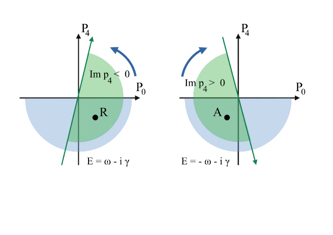
Figure 1: Clockwise and anti-clockwise Wick rotation. The anomalous pole (A) and the regular one (R) require a clockwise and anti-clockwise Wick rotation, respectively. The shaded areas are the contours which must be chosen for $t>0$ in the Fourier transform, according to Jordan lemma.

3.2 clockwise and anti-clockwise rotation

The opposite sign of the anomalous part can be understood by the same convergence principle, requiring a finite outcome for any physical observable or any physical quantity, like the gluon propagator, which seems to be strongly related to physical observables, as discussed in the previous section. Actually, when going to the Euclidean space, the usual Wick rotation cannot be used for the anomalous part because the anomalous poles are in the wrong sectors of the complex plane and would be crossed by the usual rotation. As shown in Fig. 1, the anomalous part of the Minkowskian propagator can only be continued to the Euclidean space by a clock-wise rotation, which by Jordan’s lemma yields the correct (finite) analytic continuation provided that a negative imaginary time $\tau<0$ is associated to a positive real time $t>0$. In more detail, taking $p_{0}=ip_{4}$ and $t=-i\tau$, the direct-space propagator is defined, as a function of time, by a Fourier transform with an exponential which reads

$$e^{\displaystyle{ip_{0}\,t}}=e^{\displaystyle{ip_{4}\,\tau}}.$$ (15)

In the transform, the contour integral is finite if and only if $t>0$ when $\mathop{\rm Im}{p_{0}}<0$ and $\tau>0$ when $\mathop{\rm Im}{p_{4}}<0$. Thus, as shown in the figure and discussed in Ref.[9], the clockwise rotation leads to the opposite imaginary-time ordering for the anomalous part. Moreover, the reversed integration from $+\infty$ to $-\infty$, along the $p_{4}$ axis, leads to a change of sign for the anomalous part. Thus, the untrivial analytic continuation of the Minkowskian propagator yields the Euclidean pole part in Eq.(1), with the correct sign.

4 Conclusions

In favour of the genuine nature of the poles, we reported their gauge invariance and their physical role in determining the short-range string tension, condensates and, of course, the dynamical mass and damping of a gluon. Thus, unless we accept that the real-time propagator does not even exist[13], the analytic continuation of the gluon propagator must be deeply revised[9], leading to an effective Minkowskian propagator which is not given by the trivial analytic continuation of the Euclidean function. As shown in [9], the resulting Minkowskian propagator would be imaginary and defines an added spectral density which generalizes the Källén-Lehmann representation and might improve the reconstruction of the propagator by spectral methods.

References

- [1] M. Stingl, Phys. Rev. D 34, 3863 (1986); Erratum-ibid. D 36, 651 (1987); Z. Phys. A 353, 423 (1996).
- [2] D. Dudal, J. A. Gracey, S. P. Sorella, N. Vandersickel, and H. Verschelde, Phys.Rev. D 78, 065047 (2008).
- [3] F. Siringo, Nucl. Phys. B 907, 572 (2016); Phys. Rev. D 94, 114036 (2016).
- [4] D. Binosi and R.-A. Tripolt, Phys. Lett. B 801, 135171 (2020).
- [5] Y. Hayashi and K.-I. Kondo, Phys. Rev. D 99, 074001 (2019); Phys. Rev. D 101, 074044 (2020).
- [6] F. Siringo and G. Comitini, Phys Rev. D 98, 034023 (2018).
- [7] A. G. Duarte, O. Oliveira, P. J. Silva, Phys. Rev. D 94, 014502 (2016).
- [8] F. Siringo, Phys. Rev. D 96, 114020 (2017).
- [9] F. Siringo, G. Comitini, arXiv:2210.11541.
- [10] F. Siringo, G. Comitini, Phys. Rev. D 106, 076014 (2022).
- [11] F. Siringo, EPJ Web of Conferences 137, 13017 (2017).
- [12] Ph. Boucaud, A. Le Yaouanc, J.P. Leroy, J. Micheli, O. Pene, J. Rodriguez-Quintero, Phys. Lett. B 493, 315-324, (2000).
- [13] Y. Hayashi and K.-I. Kondo, Phys. Rev. D 103, L111504 (2021).