Path Planning Under Uncertainty to Localize mmWave Sources

Abstract

In this paper, we study a navigation problem where a mobile robot needs to locate a mmWave wireless signal. Using the directionality properties of the signal, we propose an estimation and path planning algorithm that can efficiently navigate in cluttered indoor environments. We formulate Extended Kalman filters for emitter location estimation in cases where the signal is received in line-of-sight or after reflections. We then propose to plan motion trajectories based on belief-space dynamics in order to minimize the uncertainty of the position estimates. The associated non-linear optimization problem is solved by a state-of-the-art constrained iLQR solver. In particular, we propose a method that can handle a large number of obstacles ($\sim 300$) with reasonable computation times. We validate the approach in an extensive set of simulations. We show that our estimators can help increase navigation success rate and that planning to reduce estimation uncertainty can improve the overall task completion speed.

I Introduction

Wireless communications play an important role in robotics, typically to operate robots [1] or drones [2] remotely. Additionally, wireless signals can be used as sensors, for example to localize a robot or to perform SLAM based on the signal strength of a WiFi network [3]. However, traditionally wireless signals do not contain direction information to estimate the location of the emitter precisely. The emergence of directional millimeter wave (mmWave) bands, which are deployed for example in 5G networks, have attracted significant attention for high precision localization applications. Indeed, the estimation of the direction of transmission is greatly simplified as angular information does not need to be reconstructed by complex algorithm as in [4, 5, 6].

In this paper, we study a scenario where a robot seeks to navigate to fixed but unknown mmWave wireless emitter location in an unknown environment. This could model, for example, a search and rescue scenario where the stranded human carries the emitter [7, 8, 9, 10]. Our goal is to exploit the directionality of mmWave wireless to devise a planning and estimation framework for fast navigation to the emitter.

Recent work [11] has addressed this problem using a simple navigation algorithm that follows the angle of arrival (AoA) of the received mmWave signal till the robot reaches the emitter. The algorithm can be used if the robot is in line of sight (LOS) or in non-line of sight (NLOS) settings of the emitter. However, this method has two drawbacks. First, it uses noisy, unfiltered AoA measurements and is thus ineffective when the robot is two or more reflections from the emitter. Second, it does not maintain an estimate of the transponder position, requiring the robot to navigate first to the point of reflection in NLOS settings.

This paper aims to improve upon the state-of-art using joint estimation and trajectory planning algorithms. We consider unexplored cluttered environments with possibly high degrees of signal reflections (NLOS). We propose an Extended Kalman Filter (EKF) to estimate the robot position with respect to the emitter in the LOS and NLOS cases. The filters are able to robustly estimate the direction of the wireless sources despite noisy observations. We formulate a trajectory optimization problem based on belief-space dynamics following [12] to minimize the uncertainty of the estimate along the trajectory while avoiding obstacles.

We propose an improved algorithm compared to [12] by formulating the trajectory optimization problem as a constrained one. This renders the need for expensive second-order derivatives of the cost terms when including collision avoidance unnecessary. Solvers have been proposed that are able to consider box constraints [13], or nonlinear inequality constraints for example by the augmented Lagrangian method [14] or the interior-point-method [15]. Furthermore, we provide explicit computations of the partial derivatives of the estimation covariance updates of the EKF, necessary for the solvers. This brings computational advantage compared to numerical derivatives previously reported [12]. The proposed method is evaluated using the ’Active Neural-SLAM’ framework[16], a modular, open-source, approach for mobile navigation, and demonstrate its performance benefits over prior work in a wide range of simulated indoor navigation environments.

In the following, we formulate the EKF transition and observation models for the LOS and first- and general n-th order NLOS cases (Sec. II). To obtain trajectories that minimize the uncertainty of the EKF state estimate we formulate a non-linear constrained trajectory optimization problem (Sec. III). Based on Bayesian filtering, we require the gradient of the EKF which is detailed in App. A. We start the evaluation (Sec. V) by verifying the identification based on the EKF (Sec. V-A) and path planning through cluttered environments (Sec. V-B) in simple scenarios. The methods are then applied on complex maps, with detailed results on a single typical map (Sec. V-B), and success rate and time-to-target evaluations on 200 different scenarios (Sec. V-D).

II Extended Kalman filter for transponder localization

In this section we describe the filter used to estimate the location of the robot with respect to the wireless emitter. We need to distinguish several cases depending on whether the received signal comes from an emitter in LOS, in first-order NLOS (i.e. when there was only one reflection) or in n-th order NLOS. We can use results from [11] to classify received signals accordingly.

We design several EKFs governed by nonlinear observation and process models

$$x_{i} =f(x_{i-1},u_{i})+w_{i}\quad\text{and}\quad z_{i}=h(x_{i})+v_{i}$$ (1)

where $u$ is the control, $x$ the state and $z$ the measurement. Both the state and observation are subject to Gaussian white noise processes $w$ and $v$ with covariances $W$ and $V$. The estimate of the state $x_{i|j}$ at control iteration $i$ given observations up to time $j\leq i$ and the corresponding estimation covariance $P_{i|j}$ are updated by the Kalman equations (see App. A for explicit computations of the derivatives of the estimation covariance) with first-order linearizations of the non-linear models $f$ and $h$.

We assume a Cartesian 2D planar coordinate system and aim to identify the robot position $p$ with respect to a signal emitting transponder $p_{tx}$. Due to the directional character of the mmWave band this implies that the robot can directly infer the AoA $\alpha$ of the received signal. In the following, lower indices $a_{x}$ and $a_{y}$ represent the $x$ and $y$ component of a 2D position vector $a$.

II-A Line-of-sight case

In this case we receive the signal directly from the emitter without any reflection. We identify the transponder as the origin of the coordinate system. The robot position $p$ is chosen as the filter state $x\coloneqq p$. We assume simple integrator dynamics for the mobile robot

$$p_{i+1}=p_{i}+u_{i}$$ (2)

We then write the observation model as

$$z_{i}=\begin{bmatrix}\cos(\alpha_{i})&\sin(\alpha_{i})\end{bmatrix}^{T}\quad\text{and}\quad h(x_{i})=\begin{bmatrix}\frac{p_{x,i}}{\|p_{i}\|}&\frac{p_{y,i}}{\|p_{i}\|}\end{bmatrix}^{T}$$ (3)

We chose a redundant representation to avoid discontinuities for example associated with the $\arctan$ [5]. Note however that we measure directly $\alpha_{i}$.

II-B First order non-line-of-sight

In the first-order NLOS case the received signal has been reflected one time. The reflection can be represented by

$${(p_{r}-p_{tx})^{T}}\hat{s}/{\|p_{r}-p_{tx}\|}=-{(p_{r}-p)^{T}}\hat{s}/{\|p_{r}-p\|}$$ (4)

where $p_{tx}$ is the transponder position in some global reference system. $p_{r}$ is the point of reflection (POR) which lies on the line of reflection (LOR)

$$s=\begin{bmatrix}0&c\end{bmatrix}^{T}+t\hat{s}\qquad\text{with }\hat{s}=\begin{bmatrix}1&m\end{bmatrix}^{T}$$ (5)

$c$ is the offset along the $y$-axis and $m$ is the inclination of the LOR. The two dimensions of $p_{r}$ are linearly dependent

$$p_{r,y}=mp_{r,x}+c$$ (6)

Together with (4) we can derive a symbolic expression for $p_{r,x}=f(p,p_{tx},m,c)$. The observation model becomes then (we use the same state $z_{i}$ as in (3))

$$h(x_{i})=\begin{bmatrix}\frac{p_{r,x,i}-p_{x,i}}{\|p_{r,i}-p_{i}\|}&\frac{p_{r,y,i}-p_{y,i}}{\|p_{r,i}-p_{i}\|}\end{bmatrix}^{T}$$ (7)

We need to distinguish two cases, depending on whether we know the line of reflection.

II-B1 Unknown line of reflection

In case that the LOR is unknown we place the origin of the coordinate system at the transponder ($p_{tx}=0$). The filter states are $x\coloneqq\begin{bmatrix}p^{T}&m&c\end{bmatrix}^{T}$. We use the same dynamics for $p$. The dynamics of $m$ and $c$ are just random noise. We see that this filter will have observability issues to identify $m$ and $c$ and will need a good initial estimate of the LOR. In the following we propose instead to estimate the LOR from the current state of the visual SLAM algorithm.

II-B2 Known line of reflection

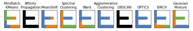
Figure 1: Clustering methods on a map with three walls. Clustering based on the Gaussian Mixture model leads to a clean separation between the different wall segments.

We parametrize walls by LOR’s from a 2D point map of the environment (identified for example by some SLAM modality) using a clustering and regression process. We first identify clusters in order to separate walls from each other, for example if two walls form a corner. Figure 1 depicts the results from a clustering process of a point cloud representing three intersecting walls using different methods. We decided to use clustering based on a Gaussian mixture model with Bayesian estimation of a Gaussian mixture [17] as it led to the best separation of the walls in our experiments. In a second step, we use linear regression to fit the LOR’s (6) to the identified point clusters.

The filter is accordingly formulated in the global SLAM reference system. Therefore, $p_{tx}$ needs to be identified while we use the current SLAM estimate of $p$. The corresponding filter states are then

$$\begin{bmatrix}p_{i+1}&p_{tx,i+1}\end{bmatrix}^{T}=\begin{bmatrix}p_{i}+u_{i}&p_{tx,i}\end{bmatrix}^{T}$$ (8)

II-C $n$-th order non-line-of-sight

The first-order NLOS formulation can be extended to $n$-th order by defining $n$ LOR’s $\hat{u}_{k}=\begin{bmatrix}1&m_{k}\end{bmatrix}^{T}$ with known reflection order $k=1,\dots,n$. For each LOR the equation

$$\frac{(p_{r,k}-p_{r,k-1})^{T}}{\|(p_{r,k}-p_{r,k-1})\|}\hat{u}_{k}=-\frac{(p_{r,k}-p_{r,k+1})^{T}}{\|p_{r,k}-p_{r,k+1}\|}\hat{u}_{k},\text{ }k=1,...,n$$ (9)

describes the incoming and outgoing rays at the $k$-th reflection point $p_{r,k}$. We have $p_{r,0}=p_{tx}$ (transponder position) and $p_{r,n+1}=p$ (robot position). This leads to an expression for $p_{r,n,x}=f(p,p_{tx},m,c)$ with $p_{r,n,y}=m_{n}p_{r,n,x}+c_{n}$. The observation model is then the same as in (3) with $p_{r,n}$ instead of $p_{r}$.

This filter requires the knowledge of the $n$ LOR’s and their correct order. We wrote the filter for completeness but in practice this is an unlikely assumption. In this work, we rather reply on an exploration mode to escape such high-order reflections, see sec. IV

III Constrained path planning under uncertainty

We now present the trjectory optimization approach. Our goal is to compute paths that will move the robot towards the estimated emitter position while avoiding obstacles but that will additionally try to minimize the predicted uncertainty on these estimates. We want to find paths that will take into account estimation uncertainty to improve overall navigation.

In order to receive AoA measurements that lead to EKF state estimates with minimal uncertainty we formulate the following trajectory optimization problem

$$\operatorname*{min.}_{x,u}\qquad\gamma_{N}(x_{N|N},u_{N})+\sum_{i}^{i+N-1}\gamma_{i}(x_{i|i},u_{i})$$ (10)

$$x_{i|i}\coloneqq\begin{bmatrix}p_{i|i}^{T}&\text{vec}(P_{i|i})^{T}\end{bmatrix}^{T}\leftarrow\text{EKF}(x_{i-1|i-1},u_{i})$$ (11)

$$\phi_{i}(x_{i-1|i-1},u_{i})\leq 0\qquad\text{with }i=1,...,N$$ (12)

This is a non-linear optimal control problem over a control horizon of length $N$ where we aim to minimize a cost composed of running $\gamma_{i}$ and terminal $\gamma_{N}$ costs. We aim to find for each time step $i$ of the planning horizon states $x_{i|i}$ and controls $u_{i}$ that minimize this cost while satisfying the constraints $\phi_{i}$. The state $x_{i|i}$ is comprised of the robot position estimate $p_{i|i}$ and the associated vectorized estimation covariance $P_{i|i}$ and is governed by the EKF update equations (16) for the state and covariance as a Bayesian filtering process [12]. The transition and observation matrices are chosen according to the LOS or NLOS expressions derived in Sec. II-A and Sec. II-B.

The cost $\gamma$ incorporates the distance between estimated and desired robot position $p_{i|i}$ and $p_{d}$, the uncertainty $P_{i|i}$ of the position estimate $p_{i|i}$ and the control effort $u$, all subject to minimization. The explicit formulation for the running and terminal costs then becomes

$$\gamma_{i}=u_{i}^{T}R_{i}u_{i}+tr(P_{i|i}T_{i})$$ (13)

$$\gamma_{N}=(p_{N|N}-p_{d})^{T}Q_{N}(p_{N|N}-p_{d})+tr(P_{N|N}T_{N})$$

$Q$, $R$ and $T$ are diagonal weight matrices which let us trade-off the three different objectives.

We impose lower and upper bound constraints $\underline{u}$ and $\overline{u}$ on the controls. Different from the original formulation [12], we formulate obstacle avoidance as a constraint. This is computationally advantageous as the need for second-order derivatives in iLQR [13] is rendered unnecessary. We have

$$\phi_{\text{obs},i}(x_{i|i})\coloneqq-d_{\text{euc},i}(p_{i|i})+r_{\text{rob}}+r_{\text{obs}}+n_{std}\max(\text{eig}(P_{i|i}))\leq 0$$ (14)

$d_{\text{euc}}$ is the Euclidean distance between the robot and obstacle center which are both modeled as spheres with radii $r_{\text{rob}}$ and $r_{\text{obs}}$. $\max(\text{eig}(P_{i|i}))$ is the distance along one standard deviation and gives the constraint the character of a chance constraint $P(\phi(x,u)\leq 0)\geq 0.997$ (for $n_{std}=3$).

We use the interior point method based iLQR solver IPDDP [15] to solve the problem (10) as it enables to easily include these constraints. The solver requires the gradient of both the dynamics and the constraints $\phi$. The gradient of the Bayesian filtering can be determined analytically. The gradient of the state estimation update (16) is direct and depends on the chosen state transition $f(p)$. The gradient of the estimation covariance update (16) is more involved and detailed in App. A. Finally, the analytical gradient of the obstacle avoidance constraints including the covariance term (14) can be determined according to [18]. Thanks to this formulation, we have a lower computational complexity than the original algorithm [12] as summarized in Table 1.

Method	$\nabla_{x}f(x)$ (11)	$\nabla^{2}_{x}\phi(x)$ (14)
Ours	$O(l^{4})$	not necessary
[12]	$O(l^{6})$	$O(ol^{2})$

TABLE 1: Computational comparison for selected operations per solver step according to [12] and our method based on constrained iLQR. $o$ is the number of obstacles.

IV Overall algorithm

The overall algorithm consists of two steps:

• Estimation step updates a list of EKF’s (LOS and NLOS) during the motion of the robot while observing the AoA of the received wireless signal in order to identify the approximate robot and transponder positions. New NLOS filters are added as soon as a new LOR is identified.

• Path planning step re-computes an optimize path for the robot towards the goal location $p_{d}\coloneqq p_{tx,i|i}$ based on the current estimates of the robot and transponder positions $p_{i|i}$ and $p_{tx,i|i}$ and the obstacle map.

As in our previous work [11], the algorithm is incorporated into the Neural-Slam [16] system which returns a robot position estimate $p_{i|i}$ in a 2D binary point map of the environment (free space and obstacles) using vision. We use the 2D map to generate LOR’s. A simple heuristic is used to cover the point cloud with circles which act as a convex approximation of the obstacles for the trajectory optimization.

The high-level control architecture for moving the robot to an unknown transponder position $p_{tx}$ with the current estimate $p_{tx,i|i}$ is described below. We use the machine learning based link state estimator from [11] for identifying the degree of reflection of the received wireless signal.

IV-1 LOS

the path planner uses the EKF formulation from Sec. II-A for the dynamics (11). If the Mahalanobis distance [19] of the filter is below a threshold, we plan a trajectory from the current robot position estimate $p_{0}=p_{i|i}$ to the transponder estimate with a low weight $T$ on the covariance minimization term of (10). Otherwise we choose a high weight.

IV-2 First-order NLOS

the path planner uses the EKF formulation from Sec. II-B for the dynamics (11). We check whether a virtual ray along the current received wireless signal’s AoA $\alpha$ intersects with one of the identified LOR’s. If this is the case its parametrization is used for the EKF. If several LOR’s are intersecting we choose the closest LOR. The initial position is set to the current Neural-Slam estimate $p_{0}=p_{i|i}$. The goal location is set to an offset position from the POR $p_{r}$ towards the transponder position estimate $p_{tx,i|i}$ of the EKF. This is necessary as the EKF can identify the correct distance to the LOR only if a good initial estimate exists (see Sec. V-A below).

IV-3 First-order NLOS without intersecting wall, higher-order reflections, no signal

We switch to the random exploration mode presented in [16] until the robot has approached an area with good signal reception.

V Evaluation

We conduct simulations using the AI Habitat robotic simulator [20] with environments from the Gibson 3D indoor models [21] including 3D camera data. The AoA from the mmWave signals is computed offline using ray-tracing with resolution of 1 m (cf. [11] for more details on the wireless simulation). We compute a new control trajectory every 10 control cycles. We choose the weights in the cost function $l$ (10) as $Q_{N}=50I$ for the terminal state cost, $R=0.01I$ for the running control cost and $T=50I$ for the running and terminal covariance term ($T=I$ for LOS EKF with low Mahalanbois distance $<0.1$ and $T=0$ if no covariance minimization is desired). The control limit is $\bar{u}=1$m.

First, we test the LOS and NLOS EKF’s for robot and transponder position identification on simple maps. We proceed with the evaluation of the path planner in a cluttered environment with three obstacles (sec. V-B). We continue with the transponder localization problem on a complex, cluttered environment. Finally, we evaluate the entire system in 200 different indoor scenarios and compare the performance with the previous system[11].

V-A Identification: Localization on simple maps

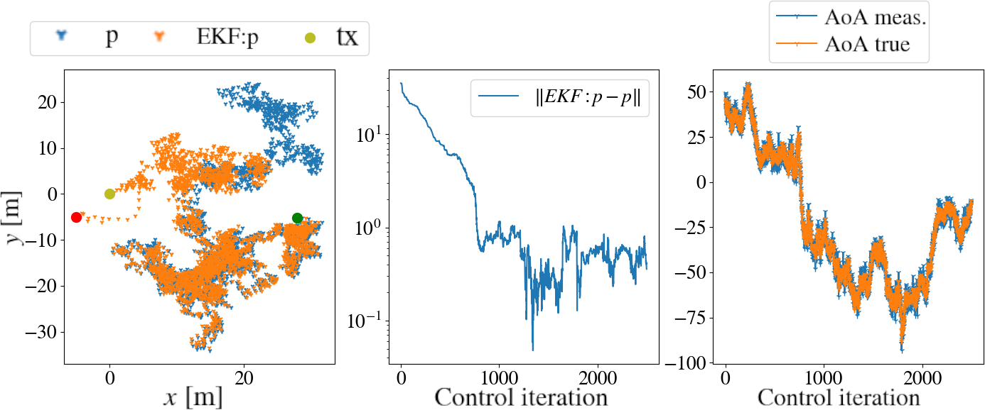
Figure 2: LOS: The filtered position $\text{EKF}\colon p$ (from red to green dot) converges to accuracy of approximately 1m. The robot receives a noisy measurement (meas.) of the signal’s AoA (true AoA in orange).

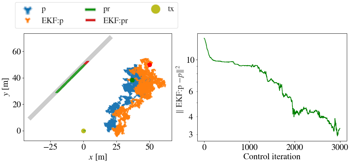
Figure 3: EKF for NLOS with known LOR. The EKF state $\text{EKF}\colon p$ converges to a point on the connecting line between the true POR $p_{r}$ and $p$.

The robot executes random motions in both $x$ and $y$ direction to gather AoA data with added Gaussian noise $\alpha+0.05w$ rad with normal distribution $w\sim\mathcal{N}(0,1)$. The filter behavior for the LOS case is depicted in Fig. 2. The received true and noisy AoA of the signal is given in the right upper graph. From the left and middle graphs it can be observed that the filtered robot position $\text{EKF}\colon p$ (orange) converges from the initial estimate with 40 m error (red) to the true one (blue) within 1 m error at the green point which corresponds to the resolution of the simulated wireless data.

An EKF convergence example for the NLOS case with a known LOR is given in Fig. 3. The position error is reduced from 10 m to 3 m. The badly identified absolute distance to the POR can be explained by the high non-linearity of the observation model. Improvements may be achieved by augmenting the observations, for example with the signal strength and a corresponding signal strength decay model. Another possibility would be to use a particle filter to obtain good initial EKF estimates [5]. Nevertheless, as we will see later, the good directional estimates are sufficient to navigate the robot to the transponder in our experiments.

V-B Evaluation of path planning

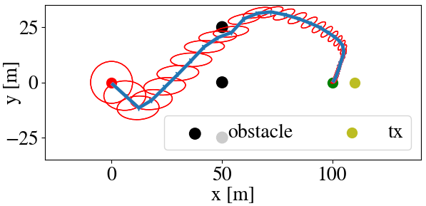
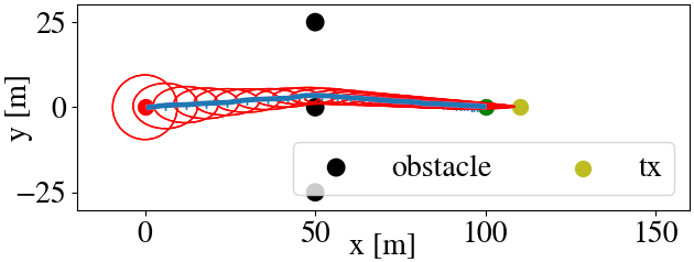
(a) LOS, $T=50I$	(b) LOS, $T=0$
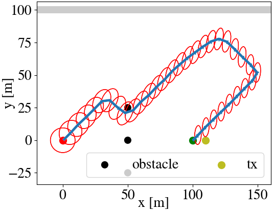
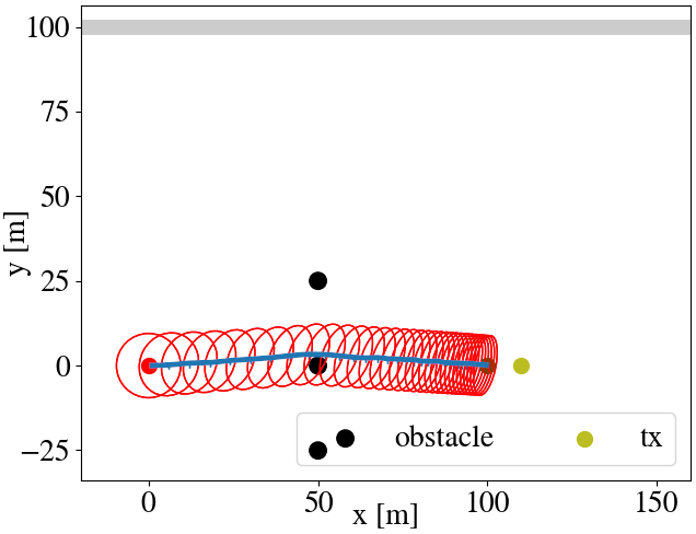
(c) NLOS, $T=50I$	(d) NLOS, $T=0$

Figure 4: Computed trajectory with obstacle avoidance. The uncertainty of the state estimate is reduced significantly for the LOS case and moderately for the NLOS case as can be seen from the red confidence ellipses along the trajectories. The LOR for the NLOS case is depicted in gray.

To illustrate how the trajectory optimization algorithm can find paths that reduce expected uncertainty, we present results in an environment with three obstacles for the LOS (sec. II-A) and NLOS (sec. II-B) case (Fig. 4). The robot is asked to move from the origin $\begin{bmatrix}0&0\end{bmatrix}$ m to the location $\begin{bmatrix}100&0\end{bmatrix}$ m while navigating three obstacles. The transponder is located at $\begin{bmatrix}0&110\end{bmatrix}$ m. In the NLOS case, the LOR is defined by $m=0$, $c=100$ m. The covariance along the path of length $N=100$ is initialized as $P=0.1I$ at each collocation point such that $\Xi\coloneqq\sum_{i=1}^{N}tr(P_{i|i})=20$. The results on the covariance are summarized in Table 2.

For $T=50I$ the trajectory optimization results in non-trivial trajectories that minimize the uncertainty of the state estimate. In the LOS case (Fig. 4a), we see a clear reduction in the uncertainty of the state estimate along the trajectory. When ignoring uncertainty reduction (zero weight $T=0$ on the covariance cost function) we find a shorter path but higher uncertainty (Fig. 4b). For the NLOS case, the reduction is less pronounced (Fig. 4c) but still visible. We explain this by the high non-linearity of the NLOS model which makes it more difficult for the solver to find a good minimizer. In all cases, all obstacles are avoided.

Case	$T=50I$	$T=0I$
LOS	4.4	10.95
NLOS	10.84	12.51

TABLE 2: Value $\Xi$ as the trace of the covariance along the trajectory from initial value $\Xi=20$ to after convergence of the trajectory optimization.

V-C Overall algorithm: Locating the transponder

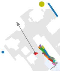
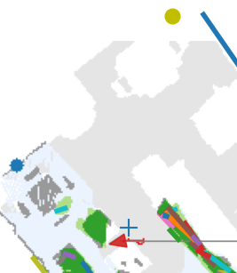
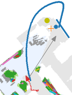
(a) Iter. 10	(b) Iter. 30	(c) Iter. 50
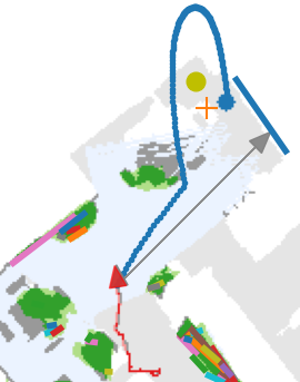
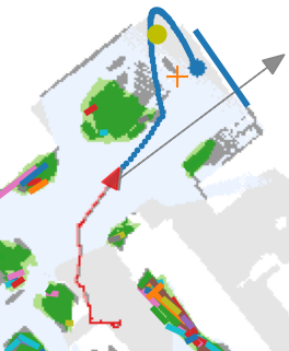
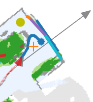
(d) Iter. 60	(e) Iter. 70	(f) Iter. 80
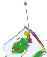
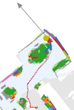
(g) Iter. 90	(h) Iter. 98

Figure 5: Path planning for transponder identification of map ’Springhill’. The point cloud identified by Neural-SLAM is shown in green and the corresponding identified LOR’s are multi-colored. The direction of the received wireless signal is indicated by the gray arrow.

We use the complete algorithm in order to navigate the robot to a previously unknown transponder position emitting a wireless signal. To illustrate a typical behavior, we present navigation results on the Gibson map ‘Springhill’ in Fig. 5. Until control iteration 40 the link-state estimator correctly informs the robot that the received signal is reflected to a high order. The exploration mode following random targets is employed. At control iteration 50, the received signal is a first-order reflection. The ray in direction of the AoA intersects with the blue wall (which we assume to be known by the robot from the beginning for demonstration purposes, despite being out of the camera’s sensing distance). The path planner computes a trajectory with horizon length of 200 to a goal offset from the LOR. This process is repeated until the robot gets in LOS with the transponder and finally arrives at the true transponder position at control iteration 98.

During the robot motion Neural-SLAM gradually constructs a point cloud (green points) of the environment. Accordingly, LOR’s are fitted to it and added to the set of EKF’s. The number of obstacles goes up to 300 as the robot progresses. Since the Hessian of the obstacle avoidance constraints is not necessary, this only leads to a slight increase of normalized computation times. The trajectory at control iteration 90 with 261 obstacles and a path length of 55 is computed in under 2 s with 122 solver iterations. The solver converges to high precision for all trajectories and all obstacles are avoided. We also notice that the resulting motions are non-trivial as they aim to reduce state covariance.

V-D Benchmark

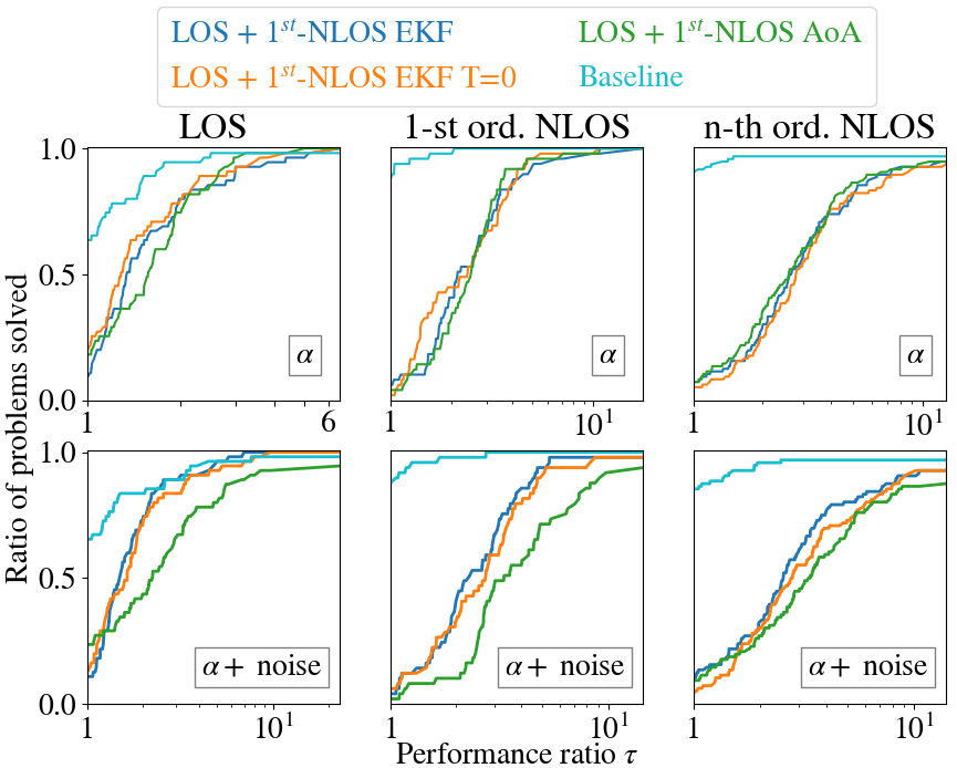
Figure 6: Performance profile for 200 transponder localization scenarios. We show the results for noise free AoA measurements (top row) and noisy AoA measurements (bottom row).

We now systematically evaluate the full system on 10 different maps with 10 different transponder locations each. We compare our algorithm with a baseline algorithm based on Neural-SLAM where the transponder positions are known in advance (pure navigation problem to a fixed desired goal). Furthermore, we show the results of the algorithm originally proposed in [11] (LOS + 1^st-NLOS AoA) which follows a target offset in the direction of the LOS or first-order NLOS AoA. Otherwise, the algorithm depends on the same exploration mode that we employ for higher-order reflections or no signal. Our algorithm is evaluated with (LOS + 1^st-NLOS EKF) and without (LOS + 1^st-NLOS EKF T=0) covariance minimization.

The results are shown in fig. 6 as the ratio of problems solved over performance ratio $\tau$ (for each solver, sum all problems’ path lengths to solution; each problem’s path length is normalized by shortest path out of all solvers). We distinguish the cases where the robot is in LOS, first-order NLOS and higher-order NLOS in the first iteration.

In the case of noise free AoA measurements all algorithms solve all problems with initial LOS or first-order NLOS configuration with a high success rate and approximately in the same time (top row). However, the pre-computed AoA arrival data from the ray-tracer can be considered ‘perfect’ simulated data. We therefore consider the case of the AoA measurements being subject to additional white noise ($w\sim\mathcal{N}(0,1)$, $\alpha+0.35w$ rad). The results are given in the bottom row of fig. 6 and summarized in table 3.

Method	Success rate	Duration
LOS+1st-NLOS EKF (Ours)	94.5%	76%
LOS+1st-NLOS EKF T=0 (Ours)	94.5%	82%
LOS+1st-NLOS AoA [11]	89.5%	100%

TABLE 3: Summary of success rate and duration (overall path length to solution) of our method with respect to [11] for noisy AoA measurements.

The EKF based algorithms solve the problems both with higher success rate ($94.5\%$ of problems solved for EKF based algorithms, $89.5\%$ for AoA based algorithm) and faster arrival times / shorter overall path lengths from initial point to transponder (problems solved in $76\%$ and $82\%$ ($T=0$) of the time required for the AoA based algorithm). This can be explained by the robot efficiently following a filtered AoA direction. A slight advantage in arrival times can be identified for the EKF based algorithm with covariance minimization ($92.7\%$ of the time required for the EKF based algorithm with $T=0$) as the more expressive motions enable a faster transponder localization under noisy observations.

VI Conclusion

In this paper we proposed a method for navigating robots through cluttered environments to quickly find a wireless (mmWave) emitter. Our method consists of an estimator for the emitter location and a trajectory optimization algorithm that aims to minimize estimation uncertainty while navigating the robot. Experiments demonstrate the advantages of the approach under noisy measurements. The estimator improves navigation success rate while the trajectory planner based on belief-space dynamics improves tasks completion speed. Additionally, by formulating a constrained trajectory optimization problem with analytic gradients our algorithm is computationally efficient and can be used in an online setting. Future work will include experiments on real robots.

Appendix A Partial derivatives of estimation covariance update of the EKF

In the following we determine the partial derivatives of the estimation covariance $P_{i|i}\in\mathcal{R}^{l,l}$ updates of the EKF with respect to the previous estimated state $x_{i-1|i-1}\in\mathcal{R}^{l}$ and the previous estimation covariance $P_{i-1|i-1}$

$${\partial P_{i|i}}/{\partial x_{i-1|i-1}}\qquad\text{ and }\qquad{\partial P_{i|i}}/{\partial P_{i-1|i-1}}$$ (15)

These are necessary to solve (10) by our constrained iLQR solver. The index $i$ is the time step, for example along the control horizon. The EKF update equations are given by

$$x_{i|i}=f(x_{i-1|i-1},u_{i})+K_{i}y_{i}\quad\text{and}\quad P_{i|i}=(I-K_{i}H_{i})P_{i|i-1}$$ (16)

with

$$y_{i}=z_{i}-h(x_{i|i-1}) \quad\text{and}\quad P_{i|i-1}=F_{i}P_{i-1|i-1}F_{i}^{T}+Q_{i}$$

$$S_{i}=H_{i}\zeta_{i}+R_{i} \quad\text{and}\quad K_{i}=\zeta_{i}S_{i}^{-1}$$

$$F=\nabla_{x}f\in\mathcal{R}^{l,l} \quad\text{and}\quad H=\nabla_{x}h\in\mathcal{R}^{r,l}$$ (17)

We define $\zeta_{i}\coloneqq P_{i|i-1}H_{i}^{T}$ with symmetry of $P_{i|i-1}$.

We use the relationships for matrix derivatives given in [22, 23]. $\Pi$ is the commutation matrix for Kronecker products. The product rule and chain rule for matrix functions applies. For the partial derivative w.r.t. the state estimate we get

$${\partial P_{i|i}}/{\partial x_{i-1,i-1}}=-\left(P_{i|i-1}\otimes\left(\zeta_{i}S_{i}^{-1}\right)^{T}\right.$$ (18)

$$+\left(P_{i|i-1}^{T}\otimes S^{-1}\zeta_{i}^{T}\right)\Pi-\zeta_{i}S_{i}^{-1}\zeta_{i}^{T}\otimes\left(\zeta_{i}S_{i}^{-1}\right)^{T}$$

$$\left.-\left(\left(\zeta_{i}S_{i}^{-1}\zeta_{i}^{T}\right)^{T}\otimes S_{i}^{-1}\zeta_{i}^{T}\right)\Pi\right)^{T}{\partial H_{i}}/{\partial x_{i-1|i-1}}$$

For the partial derivative w.r.t to the previous estimation covariance we have

$${\partial P_{i|i}}/{\partial P_{i-1|i-1}}=F_{i}^{T}\otimes F_{i}^{T}-\left(F_{i}^{T}\otimes F_{i}^{T}(\zeta_{i}S_{i}^{-1}H_{i})^{T}\right.-$$

$$(H_{i}F_{i})^{T}S_{i}^{-1}\zeta_{i}^{T}\otimes(\zeta_{i}S_{i}^{-1}(H_{i}F_{i}))^{T}\left.+(\zeta_{i}S_{i}^{-T}H_{i}F_{i})^{T}\otimes F_{i}^{T}\right)$$ (19)

The partial derivatives are computed in approximately $O(l^{6})$ operations using central differences [12]. The analytic computation is of order $O(8l^{4}+13lr^{2}+14l^{2}r+2r^{3}+3l^{3})$. The leading factor for finite differences is therefore $O(l^{6})$ whereas for the analytic expression it is only $O(l^{4})$ (assuming $l>r$).

References

- [1] M. T. Tolley, R. F. Shepherd, M. Karpelson, N. W. Bartlett, K. C. Galloway, M. Wehner, R. Nunes, G. M. Whitesides, and R. J. Wood, “An untethered jumping soft robot,” in 2014 IEEE/RSJ International Conference on Intelligent Robots and Systems, 2014, pp. 561–566.
- [2] K. Li, W. Ni, and F. Dressler, “Continuous maneuver control and data capture scheduling of autonomous drone in wireless sensor networks,” IEEE Transactions on Mobile Computing, pp. 1–1, 2021.
- [3] B. Ferris, D. Fox, and N. D. Lawrence, “Wifi-slam using gaussian process latent variable models.” in IJCAI, vol. 7, no. 1, 2007, pp. 2480–2485.
- [4] Y. Zhang, A. K. Brown, W. Q. Malik, and D. J. Edwards, “High resolution 3-d angle of arrival determination for indoor uwb multipath propagation,” IEEE Transactions on Wireless Communications, vol. 7, no. 8, pp. 3047–3055, 2008.
- [5] J. Graefenstein, A. Albert, P. Biber, and A. Schilling, “Simultaneous mobile robot and radio node localization in wireless networks,” in 2010 International Conference on Indoor Positioning and Indoor Navigation, 2010, pp. 1–6.
- [6] L. Zwirello, T. Schipper, M. Harter, and T. Zwick, “Uwb localization system for indoor applications: Concept, realization and analysis,” Journal of Electrical and Computer Engineering, vol. 2012, 03 2012.
- [7] M. Silvagni, A. Tonoli, E. Zenerino, and M. Chiaberge, “Multipurpose uav for search and rescue operations in mountain avalanche events,” Geomatics, Natural Hazards and Risk, vol. 8, no. 1, pp. 18–33, 2017. [Online]. Available: https://doi.org/10.1080/19475705.2016.1238852
- [8] H. Wu, X. Mei, X. Chen, J. Li, J. Wang, and P. Mohapatra, “A novel cooperative localization algorithm using enhanced particle filter technique in maritime search and rescue wireless sensor network,” ISA Transactions, vol. 78, pp. 39–46, 2018, advanced Methods in Control and Signal Processing for Complex Marine Systems. [Online]. Available: https://www.sciencedirect.com/science/article/pii/S0019057817305633
- [9] M. Atif, R. Ahmad, W. Ahmad, L. Zhao, and J. J. P. C. Rodrigues, “Uav-assisted wireless localization for search and rescue,” IEEE Systems Journal, vol. 15, no. 3, pp. 3261–3272, 2021.
- [10] D. Barry, A. Willig, and G. Woodward, “An information-motivated exploration agent to locate stationary persons with wireless transmitters in unknown environments,” Sensors, vol. 21, no. 22, 2021. [Online]. Available: https://www.mdpi.com/1424-8220/21/22/7695
- [11] M. Yin, A. K. Veldanda, A. Trivedi, J. Zhang, K. Pfeiffer, Y. Hu, S. Garg, E. Erkip, L. Righetti, and S. Rangan, “Millimeter wave wireless assisted robot navigation with link state classification,” IEEE Open Journal of the Communications Society, 2022.
- [12] J. van den Berg, S. Patil, and R. Alterovitz, “Motion planning under uncertainty using iterative local optimization in belief space,” The International Journal of Robotics Research, vol. 31, no. 11, pp. 1263–1278, 2012. [Online]. Available: https://doi.org/10.1177/0278364912456319
- [13] Y. Tassa, N. Mansard, and E. Todorov, “Control-limited differential dynamic programming,” in 2014 IEEE International Conference on Robotics and Automation (ICRA), 2014, pp. 1168–1175.
- [14] B. E. Jackson, T. Punnoose, D. Neamati, K. Tracy, R. Jitosho, and Z. Manchester, “Altro-c: A fast solver for conic model-predictive control,” in 2021 IEEE International Conference on Robotics and Automation (ICRA), 2021, pp. 7357–7364.
- [15] A. Pavlov, I. Shames, and C. Manzie, “Interior point differential dynamic programming,” IEEE Transactions on Control Systems Technology, vol. 29, no. 6, pp. 2720–2727, 2021.
- [16] D. S. Chaplot, D. Gandhi, S. Gupta, A. Gupta, and R. Salakhutdinov, “Learning to explore using active neural slam,” in International Conference on Learning Representations (ICLR), 2020.
- [17] D. M. Blei and M. I. Jordan., “Variational inference for dirichlet process mixtures,” Bayesian analysis 1.1, 2006.
- [18] N. P. van der Aa, H. G. ter Morsche, and R. M. M. Mattheij, “Computation of eigenvalue and eigenvector derivatives for a general complex-valued eigensystem,” Electronic Journal of Linear Algebra, vol. 16, pp. 300–314, 2006.
- [19] P. C. Mahalanobis, “On the generalized distance in statistics,” Proceedings of the National Institute of Sciences (Calcutta), vol. 2, pp. 49–55, 1936.
- [20] M. Savva, A. Kadian, O. Maksymets, Y. Zhao, E. Wijmans, B. Jain, J. Straub, J. Liu, V. Koltun, J. Malik, D. Parikh, and D. Batra, “Habitat: A platform for embodied ai research,” in 2019 IEEE/CVF International Conference on Computer Vision (ICCV), 2019, pp. 9338–9346.
- [21] F. Xia, A. R. Zamir, Z.-Y. He, A. Sax, J. Malik, and S. Savarese, “Gibson env: real-world perception for embodied agents,” in Computer Vision and Pattern Recognition (CVPR), 2018 IEEE Conference on. IEEE, 2018.
- [22] K. B. Petersen and M. S. Pedersen, “The matrix cookbook,” nov 2012, version 20121115. [Online]. Available: http://www2.compute.dtu.dk/pubdb/pubs/3274-full.html
- [23] M. Brookes, “The Matrix Reference Manual [online].” [Online]. Available: http://www.ee.imperial.ac.uk/hp/staff/dmb/matrix/intro.html