Efficient Symbolic Approaches for Quantitative Reactive Synthesis
with Finite Tasks

Abstract

This work introduces efficient symbolic algorithms for quantitative reactive synthesis. We consider resource-constrained robotic manipulators that need to interact with a human to achieve a complex task expressed in linear temporal logic. Our framework generates reactive strategies that not only guarantee task completion but also seek cooperation with the human when possible. We model the interaction as a two-player game and consider regret-minimizing strategies to encourage cooperation. We use symbolic representation of the game to enable scalability. For synthesis, we first introduce value iteration algorithms for such games with min-max objectives. Then, we extend our method to the regret-minimizing objectives. Our benchmarks reveal that our the symbolic framework not only significantly improves computation time (up to an order of magnitude) but also can scale up to much larger instances of manipulation problems with up to 2$\times$ number of objects and locations than the state of the art.

I Introduction

Robots are experiencing a boom in their deployment in the real world. Application domains include warehouse, assembly, delivery, home assistive, and planetary exploration robots. As they transition from robot-centric workspaces to the unstructured environments, robots must be able to achieve their tasks through interactions with other agents while dealing with finite resources. This is a computationally challenging problem because planning a reaction for every possible action of other agents, known as the reactive synthesis problem, in face of resource constraints is expensive. The computational challenge is exacerbated in robotic manipulators where tasks are often complex and robots have high degrees of freedom. More specifically, when faced with humans, the problem becomes even more difficult because we expect robots to have meaningful interactions with us while still trying to complete their tasks.

Our approach is based on modeling the robot-human interaction with resource constraints as a quantitative two-player game. We use Linear Temporal Logic over finite trace (LTLf) [1] for precise specification of tasks that can be accomplished in finite time. Using the game-theoretic approach allows us to base our method within the reactive synthesis framework to generate correct-by-construction strategies that guarantee satisfaction of the task while enabling the robot to have meaningful interaction with the human. Specifically, we build on the results of [2], which show resource-minimizing strategies emit “unfriendly” interactions because the human is viewed as an adversarial agent, and hence, these strategies attempt to avoid the human by all means. Instead, regret-minimizing strategies, which evaluate the cost of actions in the hindsight relative to a resource budget, are “friendly” because they seek cooperation with the human up until resources are endangered. Fig. 1 illustrates robot behaviors under these strategies.

However, the challenge with regret-minimizing strategies is that they are finite-memory [2], requiring the knowledge of history to evaluate regret, leading to a computational blow-up (both in time and space) on an already-difficult problem.

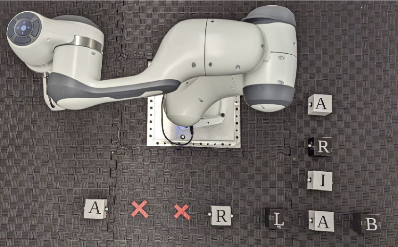
((a)) Adversarial Behavior

((b)) Regret Behavior

Figure 1: The robot is tasked with spelling “ARIA LAB” either horizontally or vertically. The white boxes are movable while the black boxes are fixed. A human can reach and move boxes placed on the left of the “L” box. (a) Resource-minimizing strategy via [3], under which the robot expends more energy to operate away from the human. (b) Regret-minimizing strategy via [2], under which the robot operates near the human to seek cooperation.

To mitigate the computational bottleneck, we propose symbolic algorithms for quantitative games. We represent the manipulation game symbolically, which significantly reduces memory usage. Further, we introduce value iteration algorithms for quantitative symbolic games with min-max objectives. Finally, we extend our symbolic approach to the regret framework in [2]. Case studies and benchmarks reveal that our symbolic framework not only significantly improves computation time (up to an order of magnitude) but also can scale up to way larger instances of manipulation problems with up to 2$\times$ number of movable objects and locations than the state of the art.

In short, the contributions of this work are fourfold:

(i) the first symbolic value iteration algorithm using the compositional encoding for two-player quantitative games, to the best of our knowledge, (ii) an efficient symbolic synthesis algorithm for regret-minimizing strategies, (iii) an open-source tool for quantitative symbolic reactive synthesis with Planning Domain Definition Language (PDDL) plug-in, and (iv) a series of benchmarks and illustrative manipulation examples that show the efficacy of the proposed symbolic framework in scaling up to real-world problems.

I-A Related Work

Reactive synthesis has recently been studied for both mobile robots [4, 5] and manipulators [6, 7]. The approaches to mobile robots are based on qualitative games. Work [8, 3] in robotic manipulation use quantitative turn-based game abstraction to model the interaction between the human and the robot. By assuming the human is adversarial, winning strategies are synthesized for the robot that guarantee task completion. While this approach has nice task completion guarantees with resource constraints, the adversarial assumption is conservative and results in one-sided, uncooperative interactions. Recently, [9] relaxed this assumption by modeling the human as a probabilistic agent. They use data gathered from past interactions to model the interaction as a Markov decision process. This approach results in better interactions, but the synthesized strategies reason about the human behavior in expectation, rather than as a strategic agent. In the most recent work [2], the notion of regret is employed to incorporate cooperation-seeking behaviors for the robot while still preserving the task completion guarantees. That approach produces “meaningful” interactions, but the robot needs to keep track of human’s past actions, leading to major computational issues.

To enable scalability of reactive synthesis, recent work [10] focuses on symbolic approaches. They use Binary Decision Diagrams (BDDs) to represent sets of states and transitions as boolean functions. With this representation, the robot can efficiently reason about the effects of its actions on the world by manipulating boolean formulas. Work [10] shows how planning with LTLf [11] symbolically allows much better scalability for qualitative manipulation games. In [12], a hybrid approach to symbolic min-max game is formulated. The states are represented explicitly, while their values are stored symbolically. Work [13] extends this framework to purely symbolic algorithms for specifications defined over the infinite horizon GR(1). Although these approaches are effective, they are limited to infinite tasks. In manipulation, however, tasks are often finite (achievable in finite time), which is the focus of this work.

II Problem Formulation

II-A Manipulation Domain Abstraction

The problem of planning for a robot in interaction with a human is naturally continuous with high degrees of freedom. Due to difficulty of reasoning in such spaces, they are commonly abstracted to discrete models [8, 2, 3, 9], known as abstraction. Similar to [2, 3], we use a two-player game abstraction to model the human-robot interaction.

Definition 1 (Two-player Manipulation Domain Game).

The two-player turn-based manipulation domain is defined as a tuple $\mathcal{G}=(V,v_{0},A_{s},A_{e},\delta,F,\Pi,L)$, where

• $V=V_{s}\cup V_{e}$ is the set of finite states, where $V_{s}$ and $V_{e}$ are the sets of the robot and human player states, respectively, such that $V_{s}\cap V_{e}=\emptyset$,

• $v_{0}\in V_{s}$ is the initial state,

• $A_{s}$ and $A_{e}$ are the sets of finite actions for the robot and human player, respectively,

• $\delta:V\times(A_{s}\cup A_{e})\to V$ is the transition function such that, for $i,j\in\{s,e\}$ and $i\neq j$, given state $v\in V_{i}$ and action $a\in A_{i}$, the successor state is $\delta(v,a)\in V_{j}$,

• $F:V\times(A_{s}\cup A_{e})\to\mathbb{R}_{\geq 0}$ is the cost function that, for robot $v\in V_{s}$ and $a\in A_{s}$, assigns cost $F(v,a)\geq 0$, and $F(v,a)=0$ for all human $v\in V_{e}$ and $a\in A_{e}$,

• $\Pi=\{p_{0},\ldots,p_{n}\}$ is set of task-related propositions that can either be true or false, and

• $L:V\to 2^{\Pi}$ is the labeling function that maps each state $v\in V$ to a set of atomic propositions $L(v)\subseteq\Pi$ that are true in $v$.

Intuitively, every state in $\mathcal{G}$ encodes the current configuration of the objects and the status of the robot. For instance, each state is a tuple that captures the locations of all the objects in the workspace and the end effector’s status as free or occupied. A successor state encodes the status of the objects and the end effector under a human or robot action.

Example 1.

Fig. 2(a) depicts a sample manipulation domain for a robot. Fig. 2(b) is its extension to a game abstraction $\mathcal{G}$ that captures the interaction between the robot and a human.

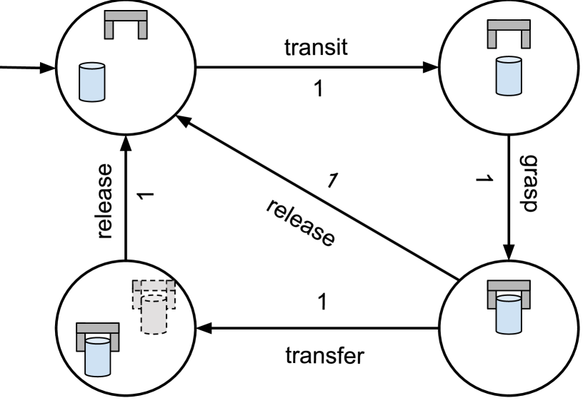
((a)) Transition System

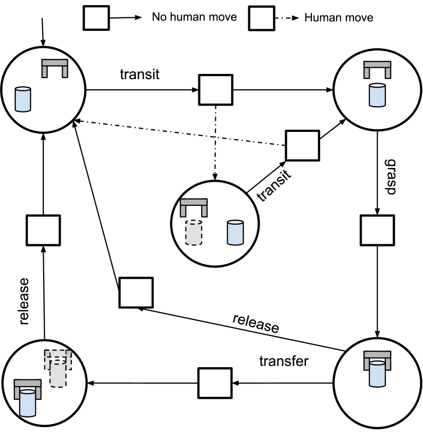
((b)) Two-player game

Figure 2: Manipulation Domain $\mathcal{G}$ for Example 1. States in circle and square belong to set $V_{s}$ and $V_{e}$, respectively.

In this game, each player has a strategy to choose actions. Robot strategy $\sigma:V^{*}\cdot V_{s}\to A_{s}$ and human strategy $\tau:V^{*}\cdot V_{e}\to A_{e}$ pick an action for the respectively player given a finite sequence of states (history). A strategy is called memoryless if it only depends on the current state. The set of all strategies for the robot and human players are denoted by $\Sigma^{\mathcal{G}}$ and $\mathrm{T}^{\mathcal{G}}$, respectively.

Given strategies $\sigma$ and $\tau$, the game unfolds, and a play $P(\sigma,\tau)=v_{0}v_{1}\ldots v_{n}\in V^{*}$, which is a finite sequence of visited states, is obtained. Intuitively, a play captures the evolution of the game (movement of the objects in the workspace) for some robot and human actions.

Each action has a cost associated with it, e.g., energy. We define the total payoff $\operatorname{Val}^{v_{0}}(P(\sigma,\tau))$ associated with a play to be the sum of the costs of the actions taken by the players, i.e.,

$$\textstyle\operatorname{Val}^{v_{0}}(P(\sigma,\tau)):=\sum_{i=0}^{n-1}F(v_{i},a_{i},v_{i+1}),$$ (1)

where $a_{i}=\sigma(v_{0}\ldots v_{i})$ if $v_{i}\in V_{s}$, otherwise $a_{i}=\tau(v_{0}\ldots v_{i})$. Further, a trace for play $P(\sigma,\tau)$ is the sequence of labels $\rho=L(v_{0})L(v_{1})\ldots L(v_{n})$ of the states of $P(\sigma,\tau)$. Intuitively, the trace represents the evolution of the manipulation domain relative to a given task.

II-B LTL over finite Trace (LTLf)

As most of robotic manipulation tasks are desired to be accomplished in finite time, a good choice to specify them unambiguously is LTLf [1]. LTLf has the same syntax as Linear Temporal Logic (LTL), but the semantics are defined over finite executions (traces).

Definition 2 (LTLf Syntax [1]).

Given a set of atomic propositions $\Pi$, LTLf formula $\varphi$ is defined recursively as:

$$\varphi:=p\;|\neg\varphi\;|\varphi\;\wedge\;\varphi\;|X\;\varphi\;\;|\varphi\,U\varphi$$

where $p\in\Pi$ is an atomic proposition, “$\neg$” (negation) and $``\wedge$” (and) are boolean operators, and “$X$” (next) and “$U$” (until) are the temporal operators.

We define commonly used temporal operators “$F$” (eventually) and “$G$” (globally) as $F\varphi:=\top\;U\;\varphi$ and $G\varphi:=\neg F\neg\varphi$.

The semantics of LTLf formulas is defined over finite traces in $\big{(}2^{\Pi}\big{)}^{*}$ [1]. Notation $\rho\models\varphi$ denotes that trace $\rho\in\big{(}2^{\Pi}\big{)}^{*}$ satisfies formula $\varphi$. We say that play $P(\sigma,\tau)$ accomplishes $\varphi$, denoted by $P(\sigma,\tau)\models\varphi$, if its trace $\rho\models\varphi$.

Example 2.

For our manipulation domain, a task to build an arch with two support boxes and one colored box on top can be expressed as, $\varphi_{\text{arch}}=F\left(p_{\text{box, support}_{1}}\land p_{\text{box, support}_{2}}\land p_{\text{green, top}}\right)\land G\left(\neg(p_{\text{box, support}_{1}}\wedge p_{\text{box, support}_{2}})\rightarrow\neg p_{\text{green, top}}\right).$

Our goal is to synthesize a strategy for the robot that can interact with the human to achieve its task $\varphi$. Specifically, we seek a strategy that guarantees the completion of $\varphi$ by using no more than a given cost (energy) budget $\mathcal{B}\in\mathbb{R}_{\geq 0}$ under all possible human actions. We refer to such a strategy as a winning strategy. Formally, robot strategy $\sigma$ is called winning if, for all $\tau\in\mathrm{T}^{\mathcal{G}}$, $P(\sigma,\tau)\models\varphi$ and $\operatorname{Val}(\sigma,\tau)\leq\mathcal{B}$.

The first problem we consider in this work is an efficient method of synthesizing a winning strategy.

Problem 1 (Min-Max Reactive Synthesis).

Given 2-player manipulation domain game $\mathcal{G}$ and LTLf task formula $\varphi$, efficiently generate a winning strategy $\sigma^{*}$ for the robot that guarantees the completion of task $\varphi$ and minimizes its required budget $\mathcal{B}$ under all possible human strategies, i.e.,

$$\sigma^{*}= \operatorname*{arg\,min}_{\sigma\in\Sigma^{\mathcal{G}}}\max_{\tau\in\mathrm{T}^{\mathcal{G}}}\operatorname{Val}^{v_{0}}(\sigma,\tau)\;\;\text{s.t. }\;P(\sigma,\tau)\models\varphi\;\forall\tau\in\mathrm{T}^{\mathcal{G}}.$$

Note that in the above formulation, the human is viewed as an adversary, i.e., it assumes human takes actions to maximize the cost budget of the robot. In the real world, however, humans are usually cooperative and willing to help. Hence, the robot strategies obtained by the above formulation are typically “unfriendly” to the human, i.e., they seek to avoid interacting with the human. Rather, we desire strategies that seek cooperation with the human while still considering that the human may not be fully cooperative.

A formulation that enables such interaction is regret-based synthesis as shown in [2]. Intuitively, regret is a measure of how good an action is relative to the best action if the robot knew the human’s reaction in advance.

Definition 3 (Regret [14]).

Under robot and human strategies $\sigma$ and $\tau$, respectively, regret at state $v\in V$ is defined as

$$\operatorname{reg}^{v}(\sigma,\tau)=\operatorname{Val}^{v}(\sigma,\tau)-\min_{\sigma^{\prime}}\,\operatorname{Val}^{v}(\sigma^{\prime},\tau),$$ (2)

where $\sigma^{\prime}$ is an alternate strategy to $\sigma$ $(\Sigma^{\mathcal{G}}\backslash\sigma)$ for the robot.

This regret definition uses best-responses, i.e., $\min_{\sigma^{\prime}}\,\operatorname{Val}^{v}(\sigma^{\prime},\tau)$, to measure how good an action is for a fixed human strategy $\tau$. Hence, the objective is to synthesize strategies for the robot that minimize its regret under the assumption that human takes action to maximize robot’s regret.

Problem 2 (Regret-Minimizing Reactive Synthesis).

Given 2-player manipulation domain game $\mathcal{G}$, LTLf task formula $\varphi$, and Budget $\mathcal{B}\in\mathbb{R}_{\geq 0}$, efficiently compute a winning strategy $\sigma^{*}$ for the robot that guarantees not only the completion of task $\varphi$ but also explores possible collaborations with the human by minimizing its regret, i.e.,

$$\sigma^{*}= \operatorname*{arg\,min}_{\sigma\in\Sigma^{\mathcal{G}}}\max_{\tau\in\mathrm{T}^{\mathcal{G}}}\operatorname{reg}^{v_{0}}(\sigma,\tau)$$

$$\text{s.t. }\quad P(\sigma,\tau)\models\varphi\qquad\qquad\quad\;\,\forall\tau\in\mathrm{T}^{\mathcal{G}}$$

$$\qquad\;\,\operatorname{Val}^{v_{0}}(\sigma,\tau)\leq\mathcal{B}\qquad\qquad\forall\tau\in\mathrm{T}^{\mathcal{G}}.$$

There are generally three major challenges in the above problems.

1. Manipulation domains are notoriously known to suffer from the state-explosion problem, i.e., given a set $L$ of locations and set $O$ of objects, the size of the abstraction is $\mathcal{O}(|L|^{|O|})$. Here, this challenge is exacerbated by considering an extension of the domain to human-robot manipulation games as well as high-level complex tasks, requiring composition of the game domain with the task space.

2. These games are quantitative, requiring to reason not only about the completion of the task but also the needed quantity (budget), which adds numerical computations to the already-expensive qualitative algorithms.

3. While memoryless strategies are sufficient for Problem 1, regret minimizing strategies (Problem 2) are necessarily finite memory [2], making the computations even more challenging.

Existing algorithms for Problems 1 and 2 are based on explicit construction of the game venue’s graph. They are hence severely limited in their scalability and cannot find solutions to real-world manipulation problems in a reasonable amount of time. In addition, for regret-minimizing strategies, the algorithms require large amount of memory (tens of GB) even for small problem instances (see benchmarks in [2]). To overcome these challenges, rather than relying on explicit construction, we base our approach on symbolic methods.

III Preliminaries

In this section, we briefly introduce the preliminaries needed for our framework. First, we review the explicit algorithm for quantitative games that solves Problem 1, and then present BDDs, which are structures used to represent boolean functions.

III-A Overview of Explicit Strategy Synthesis

DFA: The approach proposed in [3] for Problem 1 is to first construct a Deterministic Finite Automata (DFA) for a given task $\varphi$. A DFA is defined as a tuple $\mathcal{A}_{\varphi}=(Z,z_{0},2^{\Pi},\delta_{\varphi},Z_{f})$, where $Z$ is a finite set of states, $z_{0}$ is the initial state, $2^{\Pi}$ is the alphabet, $\delta_{\varphi}:Z\times 2^{\Pi}\to Z$ is the deterministic transition function, and $Z_{f}\subseteq Z$ is the set of accepting states. A run of $\mathcal{A}_{\varphi}$ on a trace $\rho=\rho[1]\rho[2]\ldots\rho[n]$, where $\rho[i]\in 2^{\Pi}$, is a sequence of DFA states $z_{0}z_{1}\ldots z_{n}$, where $z_{i+1}=\delta_{\varphi}(z_{i},\rho[i+1])$ for all $0\leq i\leq n-1$. If $z_{n}\in Z_{f}$, the path is called accepting, and its corresponding trace $\rho$ is accepted by the DFA. The DFA $\mathcal{A}_{\varphi}$ reasons over the task $\varphi$ and exactly accepts traces that satisfy $\varphi$ [1]. Thus, $\mathcal{A}_{\varphi}$ captures all possible ways of accomplishing $\varphi$.

DFA Game: Next, the algorithm composes the game abstraction $\mathcal{G}$ with $\mathcal{A}_{\varphi}$ to construct a DFA game $\mathcal{P}=\mathcal{G}\times\mathcal{A}_{\varphi}$. This DFA game is a tuple $\mathcal{P}~{}=~{}(S,S_{f},s_{0},A_{s},A_{e},F,\delta_{\mathcal{P}})$, where $A_{s}$, $A_{e}$, and $F$ are as in Def. 1, $S=S_{s}\cup S_{e}$ is a set of states with $S_{s}=V_{s}\times Z$ and $S_{e}=V_{e}\times Z$, $S_{f}=V\times Z_{f}$ is the set of accepting states, $s_{0}=(v_{0},z_{0})$ is the initial state, and $\delta_{\mathcal{P}}$ is a transition function such that $s^{\prime}=\delta_{\mathcal{P}}(s,a)$, where $s=(v,z)$, $s^{\prime}=(v^{\prime},z^{\prime})$, if $v^{\prime}=\delta(v,a)$ $a$ and $z^{\prime}=\delta_{\varphi}(z,L(v^{\prime}))$. Intuitively, $\mathcal{P}$ augments each state in $\mathcal{G}$ with the DFA state $z$ as a “memory mode” to keep track of the progress made towards achieving task $\varphi$. The DFA game evolves by first evolving over the manipulation domain $\mathcal{G}$ and then checking the atomic propositions that are true at the current state and update the DFA state accordingly.

Strategy Synthesis: The classical approach for synthesizing winning strategies $\sigma^{*}$ on $\mathcal{P}$ is to play a min-max reachability game [15, 16]. Given a set of accepting states $S_{f}$, we define operators, $\operatorname*{cPreMax}(s)$ and $\operatorname*{cPreMin}(s)$, that update the state values as follows.

$$\operatorname*{cPreMax}(s) =\max_{a}(F(s,a)+W(s^{\prime}))\quad\text{if }s\in S_{e},$$ (3)

$$\operatorname*{cPreMin}(s) =\min_{a}(F(s,a)+W(s’))\quad\text{if }s\in S_{s},$$ (4)

where $s^{\prime}=\delta(s,a)$, $W$ is a vector of state values, and $W(s^{\prime})$ is the value associated with state $s^{\prime}$. Then, the algorithm for reachability games with quantitative constraints is to compute the (least) fixed point of the operators (3) and (4) by applying the operator over all the states in $\mathcal{P}$. Thus, playing a min-max reachability game reduces to fixed-point computation and is summarized in Alg. 1 [16]. While the value-iteration algorithm for min-max reachability is polynomial [15], fixed-point computation over large graphs ($|S|$ is very large) becomes computationally expensive in terms of time and memory. To mitigate this issue, symbolic graphs are often employed where the state and transition function are represented as boolean functions. Below, we discuss how to store and manipulate the boolean functions.

1

2

3

Input : Explicit DFA Game $\mathcal{P}$

Output : Winning strategy $\sigma_{win}$, Optimal values $W$

4 $W(S)\leftarrow\infty;\quad\sigma\leftarrow\emptyset;\quad\tau\leftarrow\emptyset;\quad W^{\prime}\leftarrow\emptyset$

5 $W(S_{f})\leftarrow$ initialize all accepting state values as zero

6 while $W^{\prime}\neq W$ do

7       $W^{\prime}=W$

8       $W(s)=\textnormal{{max}}(F(s,a)+W^{\prime}(s’))\quad\forall s\in S_{e}$

9       $\tau_{s}=\textnormal{{argmax}}_{a}(F(s,a)+W^{\prime}(s’))\quad\forall s\in S_{e}$

10       $W(s)=\textnormal{{min}}(F(s,a)+W^{\prime}(s’))\quad\forall s\in S_{s}$

11       $\sigma_{s}=\textnormal{{argmin}}_{a}(F(s,a)+W^{\prime}(s’))\quad\forall s\in S_{s}$

12      

return $W$, $\sigma$

Algorithm 1 Explicit Value Iteration

III-B Symbolic Data Structures: BDDs and ADDs

Symbolic Data structures like BDDs [17, 18] have been extensively used by the model-checking and verification community due to their ability to perform fixed-point computations over large state spaces efficiently [19, 20]. BDD is a canonical directed-acyclic graph representation of a boolean function $f:2^{X}\to\{0,1\}$ where $X$ is a set of boolean variables. To evaluate $f$, we start from the root node and recursively evaluate the boolean variable $x_{i}\in X$ at the current node until we reach the terminal node. The order in which the variables appear along each path is fixed and is called variable ordering. Due to the fixed variable ordering, BDDs are canonical, i.e., the same BDD always represents the same function. The power of BDDs is that they allow compact representation of functions like transition relations and efficiently perform set operations, e.g., conjunction, disjunction, negation.

((a)) Explicit Two-player game abstraction

((b)) Symbolic Two-player game

((c)) BDD for set $V^{\prime}$

((d)) ADD for set $V^{\prime\prime}$

Figure 3: (a) and (b) illustrate explicit graph and its equivalent symbolic graph, respectively. Robot actions transit (ts) is $o_{0}\wedge o_{1}$, grasp (gr) is $o_{0}\wedge\neg o_{1}$, transfer (tr) is $\neg o_{0}\wedge o_{1}$, and release (rl) is $\neg o_{0}\wedge\neg o_{1}$. Human actions human-move (dashed) and no human-move (solid) are $i_{0}$ and $\neg i_{0}$, respectively. We skip human-move edges for simplicity. Variables $x_{0},x_{1}\in X$ correspond to robot configuration and $x_{2}\in X$ for box being grounded ($p_{00}$) or manipulated ($p_{ee}$). (c) and (d) illustrate the BDD and ADD for Example 3 and 4.

Example 3.

Consider the explicit Graph $\mathcal{G}$ in Fig. 3(a). Denote each state $v\in V$ by its corresponding boolean formula over boolean variables $X=\{x_{0},x_{1},x_{2}\}$. This is shown in Fig. 3(b). Fig. 3(c) shows the BDD corresponding to boolean function representing subset of states $V^{\prime}=\{v_{s1},v_{s4}\}$, i.e, $f(x_{0},x_{1},x_{2})=(x_{0}\wedge x_{1}\wedge x_{2})\vee(\neg x_{0}\wedge x_{1}\wedge\neg x_{2})$.

Algebraic Decision Diagrams (ADDs), also known as Multi-Terminal BDDs, are a generalization of BDDs, where the realization of a boolean formula can evaluate to some set [21]. Mathematically, ADDs represent boolean function $f:2^{X}\to C$, where $X$ is a set of boolean variables and $C\subset\mathbb{R}$ is a finite set of constants. Similar to BDDs, ADDs are also built on principles of Boole’s Expansion Theorem [22]. Thus, all the binary operations that are applicable to BDDs are translated to ADDs as well.

Example 4.

We assign, to states in $V^{\prime\prime}=\{v_{s2},v_{s5}\}$ in Fig. 3(a), integer values 2 and 3, respectively. The corresponding ADD for $f(x_{0},x_{1},x_{2})=\left((x_{0}\wedge\neg x_{1}\wedge x_{2})\to 2\right)\vee\left((\neg x_{0}\wedge\neg x_{1}\wedge\neg x_{2})\to 3\right)$ is shown in Fig. 3(d).

IV Symbolic Games

Here, we introduce symbolic graphs, their construction, and our proposed algorithms to perform symbolic Value Iteration (VI) and synthesize regret-minimizing strategies in a symbolic fashion.

IV-A Symbolic Two-player Games

To avoid explicit construction of all the states and transitions, we use a symbolic representation that lets us reason over sets of states and edges. Usually, using this approach results in a much more concise representation than explicitly representing each state and edge. However, we need to redefine algorithms to accommodate symbolic representations.

Encoding the game graph $\mathcal{G}$ using boolean formulas enables us to represent the states and actions using only a logarithmic number of boolean variables. Further, we can use BDDs (ADDs) to compactly represent these boolean formulas and perform efficient set-based operations using operations defined over BDDs (ADDs).

Definition 4 (Compositional Symbolic Game $\mathcal{G}_{s}$ [11]).

Given a Two-player game $\mathcal{G}$, its corresponding symbolic representation is defined as tuple $\mathcal{G}_{s}=(X,I,O,\eta)$ where,

• $X=\{x_{0},x_{1},\ldots,x_{n}\}$ is the set of boolean variables such that every state $v\in V$ has corresponding boolean formula whose realization is true,

• $I$ is the set of boolean variables such that every human action $a_{e}\in A_{e}$ has corresponding boolean formula whose realization is true,

• $O$ is the set of boolean variables such that every robot action $a_{s}\in A_{s}$ has corresponding boolean formula whose realization is true, and

• transition relation $\eta=\{\eta_{x_{0}},\eta_{x_{1}},\ldots,\eta_{x_{n}}\}$ is a set of boolean functions, where $\eta_{x_{i}}:2^{X}\times 2^{I}\times 2^{O}\to\{0,1\}$ such that $\eta_{x_{i}}(X,I,O)=1$ if $x_{i}\in X$ is true in the corresponding successor state, otherwise 0.

Remark 1.

Since our interest is in synthesizing a robot strategy, we do not need to compute $W$ over human states explicitly. Hence, we abstract away the states in $V_{e}$ by modifying the transitions in $\mathcal{G}$ to model the evolution from each robot state to be a function of robot action $a_{s}$ and human action $a_{e}$, i.e., $\delta:V_{s}\times A_{s}\times A_{e}\to V_{s}$ for all $v\in V_{s}$. Fig. 3(a) depicts the modified abstraction for the abstraction in Fig. 2(b).

Example 5.

For each state and action in Fig 3(a), we assign a corresponding boolean formula whose realization is set to true using variables $x\in X$, $i\in I$, and $o\in O$ as shown in Fig 3(b). Further, the transition relation $\eta$ from $v_{s1}$ and $v_{s4}$ is represented as follows. $\eta_{x_{0}}=\eta_{x_{2}}=(x_{0}\wedge x_{1}\wedge x_{2}\wedge o_{0}\wedge o_{1}\wedge\neg i_{0}).$ $\eta_{x_{0}}^{\prime}=\eta_{x_{1}}^{\prime}=\eta_{x_{2}}^{\prime}=(\neg x_{0}\wedge x_{1}\wedge\neg x_{2}\wedge\neg o_{0}\wedge\neg o_{1}\wedge\neg i_{0}).$ Thus, $\eta_{x_{0}}=\eta_{x_{0}}\vee\eta_{x_{0}}^{\prime}$, $\eta_{x_{1}}=\eta_{x_{1}}\vee\eta_{x_{1}}^{\prime}$, $\eta_{x_{2}}=\eta_{x_{2}}\vee\eta_{x_{2}}^{\prime}$, and $\eta=\{\eta_{x_{0}},\eta_{x_{1}},\eta_{x_{2}}\}$. We repeat this for all edges in $\mathcal{G}_{s}$.

Definition 5 (Symbolic DFA $\mathcal{A}_{\varphi}^{s}$).

Given DFA $\mathcal{A}_{\varphi}$, its corresponding symbolic representation is defined as tuple $\mathcal{A}_{\varphi}^{s}=(Y,X,\zeta,\mathcal{F})$, where

• $X$ is as defined for $\mathcal{G}_{s}$ in Def. 4,

• $Y=\{y_{0},y_{1},\ldots,y_{m}\}$ is the set of boolean variables such that every state $z\in Z$ has corresponding boolean formula whose realization is true,

• $\zeta=\{\zeta_{y_{0}},\zeta_{y_{1}},\ldots,\zeta_{y_{m}}\}$ is a set of boolean functions, where $\zeta_{y_{i}}:2^{X}\times 2^{Y}\to\{0,1\}$ such that $\zeta_{y_{i}}(X,Y)=1$ if $y_{i}\in Y$ is true in the successor state.

• $\mathcal{F}$ is a boolean function whose realization is true for boolean formulas corresponding $z\in Z_{f}$.

Given symbolic game $\mathcal{G}_{s}$ and DFA $\mathcal{A}^{s}_{\varphi}$, we perform value iteration symbolically as described below.

IV-B Symbolic Value Iteration (VI)

Here, we first show a VI algorithm for min-max reachability games with uniform edge weights. Then, we extend the method to arbitrary edge weights. Finally, we show how this VI for reachability games can be adapted for DFA games, hence solving Problem 1.

VI with uniform edge weights

In explicit VI in Alg. 1, at every iteration of the loop, we need to iterate through every state $s\in S$ and apply the $\operatorname*{cPreMin}$ and $\operatorname*{cPreMax}$ operators (Lines 5-8). In fact, these inner loops are performed because we need to reason over a set of states at every (outer-loop) iteration. Indeed, this procedure can be naturally encoded in a symbolic fashion, where we can efficiently perform set-based operations. As VI is essentially a fixed-point computation, where we start from the accepting states and back-propagate the state values, we need to define the predecessor operation to (i) construct the set of predecessors, and (ii) reason over them.

We define the operator that computes the predecessors as the $\operatorname*{PreImage}$ operator. Let $\omega$ be the boolean function representing a set of target states $\mathcal{F}^{\prime}$ in $\mathcal{G}_{s}$, i.e., $\omega(X):2^{X}\to 1$ for states in the target set $\mathcal{F}^{\prime}$. Now, to compute the predecessors, we use a technique called variable substitution. For each boolean variable $x\in X$ in $\omega$, we substitute the variable $x_{i}$ with its corresponding transition relation $\omega(\eta_{x_{i}})$. Variable substitution using ADDs can be implemented using the $\operatorname*{Compose}$ operator shown on Line 2 in Alg. 2. Substituting $x_{i}\leftarrow\eta_{x_{i}}$ in $\omega$ captures the value of $x_{i}$ in the predecessor states for all valid actions in $\eta_{x_{i}}$. We repeat the process for all $x_{i}\in X$ and store it as $pre$. Thus, $pre(X,I,O)$ is the new boolean function such that $2^{X}\times 2^{I}\times 2^{O}\to 1$ for the set of valid edges from states in $pre$ to a state in $\omega$.

To compute the set of winning states for a reachability game with no quantities, we perform the following procedures. First, we perform universal quantification. This preserves all the states that can force a visit to the next state. Then we existentially quantify the boolean function to compute set of states that can force a visit in one-time step. Mathematically, $\omega_{1}=\exists O\cdot(\forall I\cdot pre(X,I,O))$. We repeat this process till we reach a fixed point, i.e., $\omega_{k-1}\equiv\omega_{k}$.

To compute the winning strategies, we initialize an additional boolean function $t$ as $t(X,O)_{0}=\omega_{0}$. After each fixed-point computation, $t(X,O)_{k+1}=\forall I\cdot pre(X,I,O)_{k}$. For quantitative reachability games, we replace the universal operation with max and the existential operation with min. Thus, for a graph with uniform edge weights, this method suffices. Next, we discuss how to perform VI over $\mathcal{G}_{s}$ with arbitrary edge weights.

VI with arbitrary edge weights

Similar to the case of the uniform weights, we start with $\omega_{0}$. But instead of storing it in a monolithic boolean function, we decompose it into smaller boolean functions, each corresponding to the value associated with the states. Mathematically, $\omega_{k}=\langle B_{j}\rangle$, where $\langle B_{j}\rangle$ is a sequence of boolean functions, each representing the set of states with value $j$. For the initial iteration, $k=0$, $j=0$, and $B_{j}\equiv\omega_{0}$ is the boolean function for $\mathcal{F}^{\prime}$. To compute the predecessors, we first separate the transition relation $\eta$ according to its edge weights, i.e., $\eta=\{\eta_{c_{1}},\eta_{c_{2}},\ldots,\eta_{c_{n}}\}$, where $c_{i}$ is edge weight associated with edges in $\mathcal{G}$.

1

2

3

4

5

6

Input : vector $\langle\textnormal{{ADD}}(w_{k})\rangle$, Symbolic Game $\mathcal{G}_{s}$,

Output :  vector of pre-images $\textnormal{{ADD}}(pre)$

7 $pre=\langle\emptyset\rangle$        // vector to store predecessor as 0-1 ADDs

8 for $\textnormal{{ADD}}(B_{j})\in\textnormal{{ADD}}(w_{k})$ do

9       for $\eta_{c_{i}}\in\eta$ do

10             $j^{\prime}=j+c_{i}$

11            

12            $\textnormal{{ADD}}(B_{j^{\prime}})=\textnormal{{ADD}}(B_{j}).\textnormal{{vectorCompose}}(X,\eta_{c_{i}})$

13             $pre_{j^{\prime}}=\textnormal{{ADD}}(B_{j^{\prime}})$

14            

15      

return $\textnormal{{ADD}}(pre)$

Algorithm 2 $\operatorname*{PreImage}$

Definition 6 (Monolithic Transition Relation).

A Monolithic Transition Relation for $\mathcal{G}_{s}$ is defined as $\eta=\{\eta_{c_{i}}(X,I,O)\}$ where $\eta_{c_{i}}=\{\eta_{x}|x\in X\}$ and $c_{i}$ is an edge weight in the set of edge weights given by $F$. $\eta_{c_{i}}$ is a set of boolean functions and $\eta$ is separated based on the set of all edge weights in $\mathcal{G}$, i.e., $|\eta|=|\{F(v,a_{s})\}|$ $\forall v\in V$ and $\forall a_{s}\in A_{s}$. Further, an edge appears only once in $\eta$, i.e., $\eta_{c_{i}}(\eta_{x_{i}})\cap\eta_{c_{j}}(\eta_{x_{i}})=\emptyset$ for every $i\neq j$.

Definition 7 (Partitioned Transition Relation).

A Partitioned Transition Relation for $\mathcal{G}_{s}$ is defined as $\eta=\{\eta_{c_{i}}(X,I,O)\}$ where $\eta_{c_{i}}=\{\eta_{x}|x\in X\}$ is a set of boolean functions. Each $\eta$ is separated by robot actions $a_{s}\in A_{s}$ i.e., $|\eta|=|A_{s}|$ and $c_{i}\in\{F(v,a_{s})\}$ $\forall v\in V$ and $\forall a_{s}\in A_{s}$.

Thus, for each $\eta_{c_{i}}$ and for each $B_{j}\in\omega_{k}$, we compute the $\operatorname*{PreImage}$ of $B_{j}$ and store them as $\omega_{k+1}=\langle B_{j^{\prime}}\rangle$ where $j^{\prime}=j+c_{i}$. If $B_{j^{\prime}}$ already exists, we take the union of the boolean functions. Alg. 2 summarizes the pre-image computation over weighted edges. For strategy synthesis, we repeat the same process as above until $\omega_{k+1}\equiv\omega_{k}$, i.e., every boolean function $B_{j}$ in the $(k+1)$th iteration is $\equiv B_{j}$ in the $k$th iteration. Alg. 3 gives the pseudocode for symbolic VI with quantitative constraints. For efficient manipulation of $B_{j}$, we use ADDs. We use the $\operatorname*{Compose}$ operation for substitution, and min and max for algebraic computations.

To check for convergence, we exploit the canonical nature of ADDs for constant time equivalence checking.

1

2

3

Input : Symbolic Two-player Game $G_{s}$

Output : Winning strategy $\textnormal{{ADD}}(\sigma)$, Optimal values $\textnormal{{ADD}}(\omega_{k})$

4 $\textnormal{{ADD}}(\sigma)\leftarrow$ Initialize $\infty$ ADD

5 $\textnormal{{ADD}}(\tau)\leftarrow$ Initialize $0$ ADD

6 $\textnormal{{ADD}}(\omega_{0}),\textnormal{{ADD}}(\mathcal{F}^{\prime})\leftarrow$ Init 0-$\infty$ ADD for target states

7 $\textnormal{{ADD}}(\omega_{0})=\textnormal{{ADD}}(\omega_{0}).\textnormal{{min}}(\textnormal{{ADD}}(\mathcal{F^{\prime}}))$

8 $\textnormal{{ADD}}(\sigma)=\textnormal{{ADD}}(\sigma).\textnormal{{min}}(\textnormal{{ADD}}(\omega_{0}))$

9 while $\textnormal{{ADD}}(\omega_{k-1})\not\equiv\textnormal{{ADD}}(\omega_{k})$ do

10       $\langle\textnormal{{ADD}}(B_{j})\rangle\leftarrow\text{\small{Construct 0-1 $\textnormal{{ADD}}$s from $\textnormal{{ADD}}(\omega_{k})$}}$

11       $\textnormal{{ADD}}(pre)\leftarrow\textnormal{{preImage}}(\langle\textnormal{{ADD}}(B_{j})\rangle,G_{s})$

12      

13      $\textnormal{{ADD}}(\textnormal{{aPre}})\leftarrow$ Initialize $0$ ADD

14       for $\textnormal{{ADD}}(B_{j})\in\textnormal{{ADD}}(pre)$ do

15             $\textnormal{{ADD}}(\textnormal{{aPre}})=\textnormal{{ADD}}(\textnormal{{aPre}}).\textnormal{{max}}(\textnormal{{ADD}}(B_{j}))$

16      for $f\in 2^{I}\to 1$ do

17             $\textnormal{{ADD}}(\tau)=\textnormal{{ADD}}(\tau).\textnormal{{max}}(\textnormal{{ADD}}(\textnormal{{aPre}}).\textnormal{{restrict}}(f))$

18            

19      

20      $\textnormal{{ADD}}(\sigma)=\textnormal{{ADD}}(\sigma).\textnormal{{min}}(\textnormal{{ADD}}(\tau))$

21       for $f\in 2^{O}\to 1$ do

22             $\textnormal{{ADD}}(\omega_{k+1})=\textnormal{{ADD}}(\omega_{k}).\textnormal{{min}}(\textnormal{{ADD}}(\sigma).\textnormal{{restrict}}(f))$

23            

24      

return $\textnormal{{ADD}}(\omega_{k})$, $\textnormal{{ADD}}(\sigma)$

Algorithm 3 Symbolic Value Iteration

IV-C Strategy Synthesis for symbolic DFA Games

To synthesize symbolic winning states and strategies for the DFA game $\mathcal{P}$, we compose the $\operatorname*{PreImage}$ computation as described above to evolve over $\mathcal{G}_{s}$ and $\mathcal{A}_{\varphi}^{s}$ in an asynchronous fashion. Given a boolean function representing the set of accepting states such that $\omega_{0}(X,Y)=2^{X}\times 2^{Y}\to 1$ ($2^{X}\to 1\quad\forall v\in V$ and $2^{Y}\to 1\quad\forall z\in Z_{f}$), we first compute the predecessors over the states of $\mathcal{A}^{s}_{\varphi}$ by evolving over $y\in Y$, i.e., $pre_{\varphi}(X,Y)\leftarrow\operatorname*{PreImage}$ of $\omega_{0}(X,Y)$. This intermediate boolean function captures only the evolution of the DFA variable, i.e., $2^{X}\times 2^{Y}\to 1$ such that $2^{Y}\to 1$ for the valid DFA states in the predecessors. Finally, we evolve over the symbolic game $\mathcal{G}_{s}$ from the intermediate boolean function, i.e., $pre(X,Y,I,O)\leftarrow\operatorname*{PreImage}$ of $pre_{\varphi}(X,Y)$, to compute the boolean function representing valid predecessors in $\mathcal{G}_{s}$. Algorithmically, we modify Alg. 2 with the intermediate $pre_{\varphi}$ computation and keep the $pre$ computation consistent for evolution over $pre_{\varphi}$.

We employ the above algorithm to efficiently synthesize symbolic winning strategies for Problem 1. Our evaluations illustrate that this symbolic algorithm has an order of magnitude speedup over the explicit approach. For Problem 2, previous work [2, 14] provide algorithms for synthesizing regret-minimizing strategies for explicit graphs. Next, we discuss our efficient symbolic approach to this problem and synthesis of regret-minimizing strategies.

V Hybrid Regret synthesis algorithm

The first step in synthesizing regret-minimizing strategies is to construct the Graph of Utility $\mathcal{G}^{u}$ [2]. Intuitively, this graph captures all possible plays (unrolling) over $\mathcal{P}$ along with the total payoff associated with each path to reach a state in $\mathcal{P}$. In the explicit approach, we first construct the set of payoffs as $[B]=\{0,1,2,\ldots,\mathcal{B}\}$ where $\mathcal{B}$ is the user-defined budget. We then take the Cartesian product $\mathcal{P}\times[B]$ to construct states $(s,u)$ of $\mathcal{G}^{u}$. An edge $(s,u)\to(s^{\prime},u^{\prime})$ in $\mathcal{G}^{u}$ exists iff $(s,a,s^{\prime})$ is a valid edge in $\mathcal{P}$ and $u^{\prime}=u+F(s,a)$. As constructing $\mathcal{G}^{u}$ is Pseduo-polynomial, this computation is memory intensive.

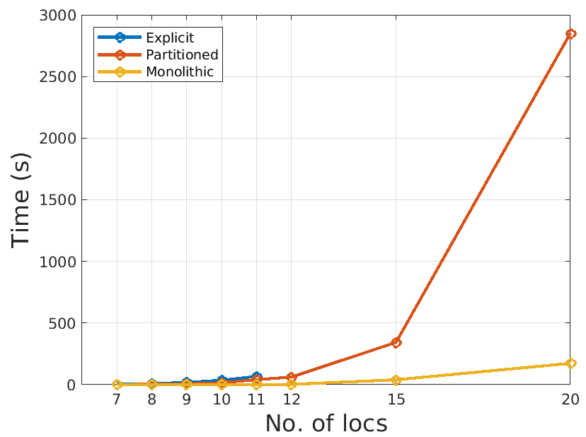
((a)) $|O|=3$ and variable $|L|$

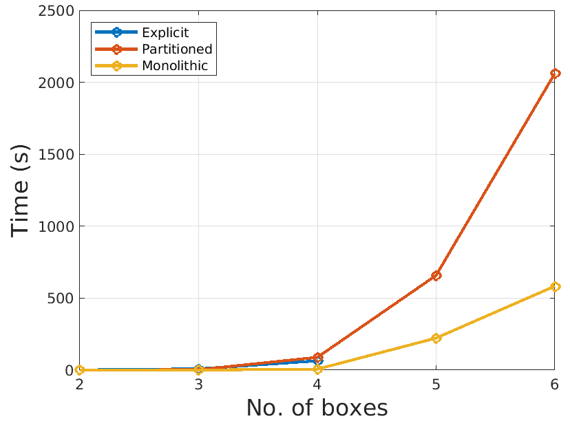
((b)) $|L|=8$ and variable $|O|$

((c)) Regret-minimizing strategy

Figure 4: (a) and (b) Benchmark results for min-max synthesis. (c) Regret-minimizing strategy for the task in Fig. 1.

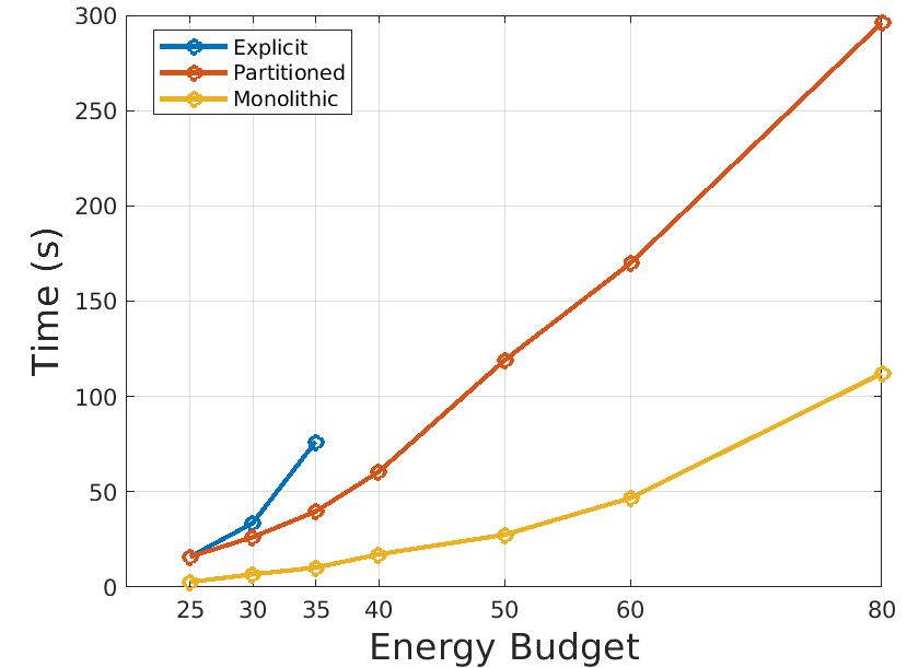
((a)) $|O|=3$, $|L|=7$, variable $\mathcal{B}$

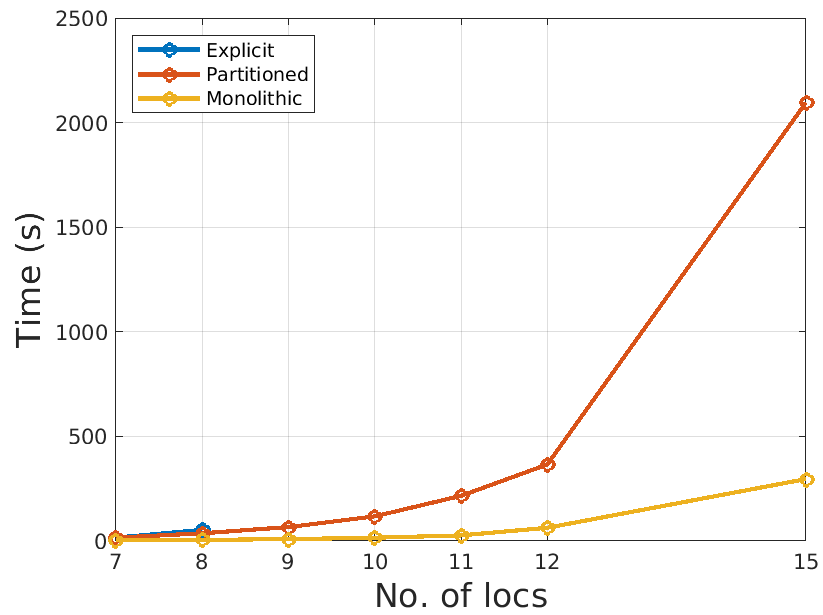
((b)) $|O|=3$, $\mathcal{B}=25$, variable $|L|$

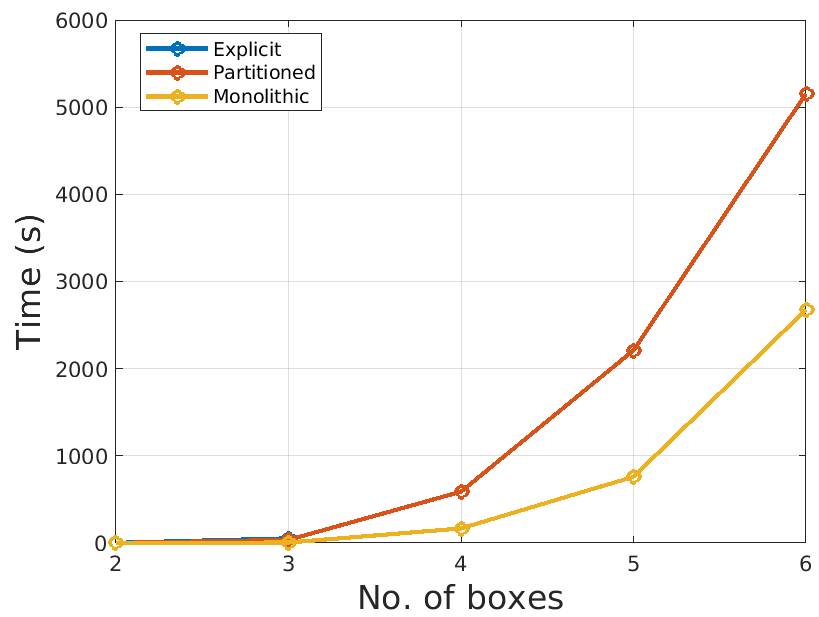
((c)) $|L|=8$, variable $\mathcal{B}$ & $|O|$

Figure 5: Benchmark results for regret-minimizing strategy synthesis in Problem 2

To construct $\mathcal{G}^{u}$ efficiently, we define $\mathcal{G}^{u}_{s}$ as the symbolic Graph of Utility. To construct the transition relation, we create an additional set of boolean variables $u\in U$ such that $2^{U}\to 1$ for valid utilities in $[B]$. We then create the transition relation $\eta_{\,\text{\scriptsize U}}$ for the utility variables to model their evolution symbolically under each action $A_{s}$. Mathematically, $\eta_{\,\text{\scriptsize U}}=\{\eta_{u_{1}},\eta_{u_{2}},\ldots,\eta_{u_{n}}\}$, where $\eta_{u_{i}}=\{\eta_{u}|u\in U\}\forall i\in n$ and $|\eta_{\,\text{\scriptsize U}}|=|\eta|$. Thus, to perform $\operatorname*{PreImage}$ operation over $\mathcal{G}^{u}_{s}$, we substitute variables $x_{i}\in X$ and $u_{i}\in U$ in a synchronous fashion using the $\operatorname*{Compose}$ operator.

The second step in regret-based synthesis is to construct the graph of the best response $\mathcal{G}^{br}$. This graph captures the best alternate payoff $ba$ from every edge along each path on $\mathcal{G}^{u}$, i.e., $\textnormal{{min}}_{\sigma^{\prime}}\operatorname{Val}(\sigma^{\prime},\tau)$ in (2). For a fixed strategy $\sigma$, we compute $ba=\textnormal{{min}}_{\sigma^{\prime}\in\Sigma^{\mathcal{G}}\backslash\sigma}\,\textnormal{{min}}_{\tau\in\mathrm{T}^{\mathcal{G}}}\,\operatorname{Val}^{(s,u)}(\sigma,\tau)$ assuming human to be cooperative (see [14] for formal definition). Finally, we repeat the process for every edge in $\mathcal{G}^{u}_{s}$ to construct the set of $ba$.

For symbolic implementation, we first compute cooperative values by first playing min-min reachability game and then “explicitly” loop over every edge in $\mathcal{G}^{u}_{s}$ to construct the symbolic transition relation for the symbolic graph of best response $\mathcal{G}^{br}_{s}$. While the computation of the $ba$ set is explicit, the resulting transition relation for $\mathcal{G}^{br}_{s}$ is purely symbolic. Finally, we play a min-max reachability game using the method described above to compute regret-minimizing strategies over $\mathcal{G}^{br}_{s}$. Our empirical results show that using this approach scales to larger manipulation problems with significantly lower memory consumption than the explicit approach.

VI Experiments

We consider various scenarios for our pick-and-place manipulation domain. We benchmark the explicit approach with the symbolic approaches from Section IV for min-max reachability games in Problem 1 and regret-minimizing strategy synthesis for Problem 2 with varying input parameters, i.e., energy budget $\mathcal{B}$, number of locations $|L|$, and number of boxes $|O|$. The task for the robot in all scenarios is to place boxes in their desired locations.

For these benchmarks, we consider the same experiments as in [2], where the robot spends 3 units of energy for every action to operate away from the human and one unit of energy when operating near the human. Refer to [2] for the experimental setup details for Problem 2. Then, we demonstrate our symbolic synthesis algorithm on the 5-box scenario in Fig. 1, on which the explicit approach runs out of memory.

Our implementation is in Python. It uses a Cython-based wrapper for the CUDD package for ADD operations [23], and MONA for LTLf to DFA translation [24]. The tool is available on GitHub [25].

Min-Max with Quantitative Constraints: For problem 1, we benchmark computation time for synthesizing winning strategies using the Explicit, Monolithic, and Partitioned symbolic approaches. For scenario 1, we fix $|O|=3$ and vary $|L|$. In scenario 2, we fix $|L|=8$ and vary $|O|$. Results are shown in Fig. 4. For the Monolithic approach, we see at least an order of magnitude speed-up over the Explicit approach for both scenarios. Further, there is almost an order of magnitude speedup for the Monolithic approach over the Partitioned approach for scenario 1. We note that the Partitioned approach is slower than the Monolithic approach due to the size of the Monolithic ADD not being large enough to compensate for the computational gain from the $\operatorname*{PreImage}$ operation over multiple smaller ADDs. Hence, the cumulative time spent computing predecessors is much more in the Partitioned approach for every fixpoint iteration than in the Monolithic approach. For the Explicit approach, we could not scale beyond 4 boxes and 8 locations due to the memory required to store $\mathcal{G}_{s}$ explicitly ($>$ 15 GB).

Regret-Minimizing Strategy Synthesis: For problem 2, we consider three scenarios. In scenario 1, we fix $|O|$ and $|L|$ and vary $\mathcal{B}$. For the scenario 2, we fix $|O|$ and $\mathcal{B}$ and increase $|L|$. Finally, for scenario 3, we fix $|L|$ and vary $\mathcal{B}$ and $|O|$. Note, for scenario 3, the regret budget $\mathcal{B}$ is chosen to be 1.25 times the minimum budget from Problem 1. Results are shown in Fig. 5. For all the scenarios, we observe that the explicit approach runs out of memory for relatively smaller instances. Additionally, we observe that overall the Monolithic approach is faster than the Partitioned approach due to the size of the Transition relation, as mentioned above.

Scalability on the Budget: Unrolling the explicit graph is a computationally intensive procedure as the state space grows linearly with budget $\mathcal{B}$. Thus, we observe in Fig. 5(a) that the explicit approach runs out of memory for $\mathcal{B}>35$. There are $62,800$ explicit nodes for $\mathcal{B}=35$ and $295,496$ explicit nodes for $\mathcal{B}=80$ in $\mathcal{G}^{br}_{s}$. We required maximum of 860 MB for the symbolic approaches and more than 9 GB for the explicit approach with $\mathcal{B}=35$.

Scalability on the number of locations: For this scenario, we observe that the Monolith approach is at least 3 times faster than the Partitioned approach. This is because, as we increase the number of locations, we do not necessarily need more boolean variables. The gap widens as we keep increasing $|L|$. For $|L|=20$, the graph has $~{}7\times 10^{6}$ nodes and $55\times 10^{6}$ edges in $\mathcal{G}^{br}_{s}$. The maximum memory consumption is $1040$ MB as opposed to over $5$ GB memory for $|L|=8$.

Scalability on the number of objects: For scenario 3, we observe that the explicit approach does not scale beyond 3 objects. The computation times for the symbolic approach also increase exponentially due to the fact that every object added to the problem instance needs an additional set of boolean variables. For $|O|=\{2,3,4,5,6\}$, we needed 29, 36, 40, 45, and 49 boolean variables with a maximum of 1100 MB consumed. The explicit approach required above 15 GB of memory for $|O|=4$.

Physical Execution: We demonstrate the regret-minimizing strategy for building “ARIA LAB” in Fig. 1. Figs. 4(c) and 1 show the initial and final configuration for $|O|=5$ (white boxes) and $|L|=7$. Robot and human cannot manipulate black boxes. We note that the human can only move the boxes in its region to its left. The robot initially operates away from the human in the robot region (yellow arrow in Fig. 4(c)). The human moves “R” (red arrow) cooperatively and allows the robot finish the task in its region (Fig. 1(b)).

Discussion: We show through our empirical evaluations that symbolic approaches can successfully scale to larger problem instances with significant memory savings. We observe that using a Monolithic representation of the transition relation is faster than the Partitioned approach due to the size of ADDs. Further, while this paper focuses on boolean representation for our problem, other ADD based optimizations like variable ordering can be utilized for a more compact representation of ADDs which could lead to additional computational speedups. Finally, we note that we compute the set of reachable states on $\mathcal{G}^{u}_{s}$ before VI. This allows the synthesis algorithm to only reason over the set of reachable states and thus speed up the synthesis process.

VII Conclusion

In this work, we provide fundamental algorithms for symbolic value iteration and symbolic regret-minimizing strategy synthesis using ADDs. We benchmark our implementation for robotic manipulation scenarios and show that we are able to achieve significant speedups. In future work, we plan to explore non-zero-sum games and alternate notions of strategies to relax the adversarial assumption and model a strategic human with their own objective.

References

- [1] G. De Giacomo and M. Y. Vardi, “Linear temporal logic and linear dynamic logic on finite traces,” in Int. Joint Conf. on Artificial Intelligence, ser. IJCAI ’13. AAAI Press, 2013, p. 854–860.
- [2] K. Muvvala, P. Amorese, and M. Lahijanian, “Let’s collaborate: Regret-based reactive synthesis for robotic manipulation,” in International Conference on Robotics and Automation, 2022, pp. 4340–4346.
- [3] K. He, M. Lahijanian, L. E. Kavraki, and M. Y. Vardi, “Reactive synthesis for finite tasks under resource constraints,” in Int. Conf. on Intel. Robots and Sys. IEEE, 2017, pp. 5326–5332.
- [4] H. Kress-Gazit, G. E. Fainekos, and G. J. Pappas, “Temporal-logic-based reactive mission and motion planning,” IEEE Transactions on Robotics, vol. 25, no. 6, pp. 1370–1381, 2009.
- [5] H. Kress-Gazit, M. Lahijanian, and V. Raman, “Synthesis for robots: Guarantees and feedback for robot behavior,” Annual Review of Control, Robot., and Auto. Sys., vol. 1, pp. 211–236, 2018.
- [6] K. He, M. Lahijanian, L. E. Kavraki, and M. Y. Vardi, “Towards manipulation planning with temporal logic specifications,” in Int. Conf. on Robotics and Automation. IEEE, 2015, pp. 346–352.
- [7] P. Hunter, G. A. Pérez, and J.-F. Raskin, “Reactive synthesis without regret,” Acta informatica, vol. 54, no. 1, pp. 3–39, 2017.
- [8] K. He, M. Lahijanian, L. E. Kavraki, and M. Y. Vardi, “Automated abstraction of manipulation domains for cost-based reactive synthesis,” IEEE Robotics and Automation Letters, vol. 4, pp. 285–292, 2019.
- [9] A. M. Wells, Z. Kingston, M. Lahijanian, L. E. Kavraki, and M. Y. Vardi, “Finite-horizon synthesis for probabilistic manipulation domains,” in IEEE International Conference on Robotics and Automation. IEEE, 2021.
- [10] K. He, A. M. Wells, L. E. Kavraki, and M. Y. Vardi, “Efficient symbolic reactive synthesis for finite-horizon tasks,” in Int. Conf. on Robotics and Automation, 2019, pp. 8993–8999.
- [11] S. Zhu, L. M. Tabajara, J. Li, G. Pu, and M. Y. Vardi, “Symbolic ltlf synthesis,” arXiv preprint arXiv:1705.08426, 2017.
- [12] K. Chatterjee, M. Randour, and J.-F. Raskin, “Strategy synthesis for multi-dimensional quantitative objectives,” Acta informatica, vol. 51, no. 3-4, pp. 129–163, 2014.
- [13] S. Maoz, O. Pistiner, and J. O. Ringert, “Symbolic bdd and add algorithms for energy games,” arXiv preprint arXiv:1611.07622, 2016.
- [14] E. Filiot, T. Le Gall, and J.-F. Raskin, “Iterated regret minimization in game graphs,” in International Symposium on Mathematical Foundations of Computer Science. Springer, 2010, pp. 342–354.
- [15] H. Gimbert and W. Zielonka, “When can you play positionally?” in Math. Found. of Comp. Sci. Springer, 2004, pp. 686–697.
- [16] T. Brihaye, G. Geeraerts, A. Haddad, and B. Monmege, “Pseudopolynomial iterative algorithm to solve total-payoff games and min-cost reachability games,” Acta Informatica, vol. 54, pp. 85–125, 2017.
- [17] F. Somenzi, “Binary decision diagrams,” NATO ASI SERIES F COMPUTER AND SYSTEMS SCIENCES, vol. 173, pp. 303–368, 1999.
- [18] R. E. Bryant, “Binary decision diagrams and beyond: Enabling technologies for formal verification,” in Int. Conf. on Computer Aided Design. IEEE, 1995, pp. 236–243.
- [19] J. R. Burch, E. M. Clarke, K. L. McMillan, D. L. Dill, and L.-J. Hwang, “Symbolic model checking: states and beyond,” Information and computation, vol. 98, no. 2, pp. 142–170, 1992.
- [20] S. Chaki and A. Gurfinkel, “Bdd-based symbolic model checking,” Handbook of Model Checking, pp. 219–245, 2018.
- [21] R. I. Bahar, E. A. Frohm, C. M. Gaona, G. D. Hachtel, E. Macii, A. Pardo, and F. Somenzi, “Algebric decision diagrams and their applications,” Formal methods in Sys. design, vol. 10, 1997.
- [22] G. Boole, The mathematical analysis of logic. Philosophical Library, 1847.
- [23] F. Somenzi, “Cudd: Cu decision diagram package 3.1.0,” University of Colorado at Boulder, 2020.
- [24] J. G. Henriksen, J. Jensen, M. Jørgensen, N. Klarlund, R. Paige, T. Rauhe, and A. Sandholm, “Mona: Monadic second-order logic in practice,” in Tools and Alg. for the Const. and Anal. of Sys. Springer, 1995, pp. 89–110.
- [25] K. Muvvala, “Symbolic reactive synthesis with quantitative objectives.” [Online]. Available: https://github.com/aria-systems-group/sym_quant_reactive_synth