Lee-Yang zeros and quantum Fisher information matrix in a nonlinear system

Abstract

The distribution of Lee-Yang zeros not only matters in thermodynamics and quantum mechanics, but also in mathematics. Hereby we propose a nonlinear quantum toy model and discuss the distribution of corresponding Lee-Yang zeros. Utilizing the coupling between a probe qubit and the nonlinear system, all Lee-Yang zeros can be detected in the dynamics of the probe qubit by tuning the coupling strength and linear coefficient of the nonlinear system. Moreover, the analytical expression of the quantum Fisher information matrix at the Lee-Yang zeros is provided, and an interesting phenomenon is discovered. Both the coupling strength and temperature can simultaneously attain their precision limits at the Lee-Yang zeros. However, the probe qubit cannot work as a thermometer at a Lee-Yang zero if it sits on the unit circle.

I introduction

The Lee-Yang zero is an interesting concept in thermodynamics, which was first proposed and discussed by Lee and Yang in 1952 Lee1952 ; Yang1952 . In the study of the lattice gas and Ising model, Lee and Yang wrote the partition function $Z$ into a polynomial form, i.e., $Z=\sum_{n}p_{n}z^{n}$, and extending $z$ to the complex plane via the analytic continuation, the roots of the equation $Z=0$ are always distributed on the unit circle. This theorem and the roots are usually referred to as the Lee-Yang unit circle theorem and Lee-Yang zeros nowadays. The Lee-Yang theorem and zeros have been widely studied in many fields, such as the field theory Simon1973 ; Fisher1978 ; Kardar2007 , condensed matterphysics Kortman1971 ; Suzuki1971 ; Lieb1981 ; Monroe1991 ; Garcia2015 ; Wei2014 ; Binek1998 ; Kim2004 ; Tong2006 ; Brandner2017 ; Lebowitz2012 ; Frohlich2012 ; Kist2021 ; Arndt2000 ; Vecsei2022 , stochastic processes Yoshida2022 ; Flindt2013 ; Deger2018 ; Deger2019 ; Deger2020 and even pure mathematics Nishimori1983 ; David2010 ; Hou2023 . In 2012, Wei and Liu proposed a remarkable scheme for the observation of Lee-Yang zeros via the dynamics of a probe qubit Wei2012 , which is then experimentally realized by Peng et al. Peng2015 in 2015. In 2019, Kuzmak and Tkachuk used a similar scheme to study the detection of Lee-Yang zeros of a high-spin system Kuzmak2019 . Moreover, the behaviors of quantum resources like spin squeezing and concurrence at the points of Lee-Yang zeros have also been investigated recently Su2020 .

The quantum Fisher information matrix is another fundamental quantity in quantum mechanics Helstrom1976 ; Holevo1982 ; Liu2020 ; Safranek2018 . It was first provided by Helstrom in the field of quantum parameter estimation, which is the extension of parameter estimation in quantum mechanics. In quantum parameter estimation, the quantum Fisher information matrix is the lower bound of the covariance matrix for a set of unknown parameters. Denote the covariance matrix as $\mathrm{cov}(\vec{x},\{\Pi_{i}\})$ with $\vec{x}$ the vector of unknown parameters and $\{\Pi_{i}\}$ a set of positive operator-valued measure, then $\mathrm{cov}(\vec{x},\{\Pi_{i}\})$ satisfies the inequality $\mathrm{cov}(\vec{x},\{\Pi_{i}\})\geq\mathcal{F}$ Helstrom1976 ; Holevo1982 , where $\mathcal{F}$ is the quantum Fisher information matrix for $\vec{x}$. The entry of $\mathcal{F}$ can be calculated via the equation $\mathcal{F}_{ij}=\mathrm{Tr}(\rho\{L_{i},L_{j}\})/2$ with $L_{i(j)}$ the symmetric logarithmic derivative for the unknown parameter $x_{i(j)}$, $\rho$ the density matrix and $\{\cdot,\cdot\}$ the anti-commutator. $L_{i}$ satisfies the equation $\partial_{x_{i}}\rho=(\rho L_{i}+L_{i}\rho)/2$. Nowadays, the quantum Fisher information matrix has been widely considered as a fundamental quantity in quantum mechanics due to its good mathematical properties and wide connections to other aspects of quantum mechanics.

It is known that the long-range Ising model can be mapped into the generalized one-axis twisting model, and thus the distribution of Lee-Yang zeros in this case are well-studied. As a matter of fact, all Lee-Yang zeros will be distributed on the unit circle in this case as long as the coefficient of the nonlinear part is negative. However, the distribution behaviors of Lee-Yang zeros for a higher nonlinearity are still unknown, even in the aspect of mathematics. To investigate it, in this paper we propose a nonlinear toy model for quantum spins and thoroughly discuss the distribution of corresponding Lee-Yang zeros, especially whether they sit on the unit circle.

Furthermore, similar to the previous studies on the detection of Lee-Yang zeros Wei2012 ; Peng2015 ; Kuzmak2019 ; Wei2017 , we also discuss the scenario that a probe qubit is coupled to the nonlinear system and show how to detect all Lee-Yang zeros by tuning the coupling strength and the coefficient of the linear part in the nonlinear system. In the meantime, due to the fact that the density matrix of this probe qubit is dependent on the temperature and coupling strength, the expression of the quantum Fisher information matrix with respect to these two parameters at the Lee-Yang zeros is analytically calculated. Through the analysis of the quantum Fisher information matrix, some interesting phenomena are discovered.

II The model and distribution of Lee-Yang zeros

Consider the following nonlinear Hamiltonian

$$\gamma H^{k}_{0}+hH_{0},$$ (1)

where $\gamma$ and $h$ are constant coefficients for the nonlinear and linear parts. $k$ is the nonlinearity. Denote $\ket{n}$ as the eigenstate of $H_{0}$ with the eigenvalue $n$. In the case that the Hamiltonian is non-degenerate, the partition function $Z=\mathrm{Tr}(e^{-\beta H})$ of this Hamiltonian can be written in a polynomial form,

$$Z=\sum_{n}p_{n}z^{n},$$ (2)

where $z=e^{-\beta h}$ and $p_{n}=e^{-\beta\gamma n^{k}}$. Here $\beta=1/(k_{\mathrm{B}}T)$ with $k_{\mathrm{B}}$ the Boltzmann constant and $T$ the temperature. In the case that the Hamiltonian is degenerate, i.e., there exist $d_{n}$ eigenstates $\ket{n_{1}},\ket{n_{2}},\dots,\ket{n_{d_{n}}}$ with respect to the eigenvalue $n$, then $p_{n}$ becomes $p_{n}=d_{n}e^{-\beta\gamma n^{k}}$. Now consider a specific Hamiltonian form

$$H=\gamma J_{z}^{k}+hJ_{z}.$$ (3)

Here $J_{z}=\frac{1}{2}\sum_{i=1}^{N}\sigma^{z}_{j}$ is the collective spin operator with $\sigma^{z}_{j}=\ket{\uparrow}\bra{\uparrow}-\ket{\downarrow}\bra{\downarrow}$ the Pauli Z matrix for the $j$th spin. The state $\ket{\uparrow}$ ($\ket{\downarrow}$) represents the spin up (down) state and $N$ is the number of spins. This Hamiltonian could be treated as the generalized nonlinear collective spin system, and when $k=2$, it is nothing but the generalized one-axis twisting model Kitagawa1993 ; Ma2011 ; Jin2009 . The physical realization of this toy model for $k\geq 3$ is still an open question for now and requires further investigation. It is easy to see that the state $\bigotimes^{N}_{j=1}\ket{a_{j}}$ ($a_{j}=\uparrow,\downarrow$) is the eigenstate of $J_{z}$ with respect to the eigenvalue $\frac{1}{2}(n_{\uparrow}-n_{\downarrow})$ with $n_{\uparrow}$ ($n_{\downarrow}$) the number of spin-up (-down) states in $\bigotimes^{N}_{j=1}\ket{a_{j}}$. As a matter of fact, another well-known representation of the eigenstate of $J_{z}$ is the Dicke state $\ket{J,m}$ and the corresponding eigenvalue is $m$. Here $J$ is the total angular momentum. Further defining $n:=m+J$ ($n=0,1,\dots,2J$), the Dicke state can be rewritten into $\ket{n}:=\ket{J,n-J}$, and the degeneracy of $\ket{n}$ is $\binom{N}{n}=\frac{N!}{n!(N-n)!}$, the binomial coefficient. Utilizing the basis $\{\ket{n}\}$, the partition function for the Hamiltonian (3) can be expressed by

$$Z=e^{\frac{1}{2}\beta hN}\sum_{n=0}^{N}\binom{N}{n}e^{-\beta\gamma\left(n-\frac{N}{2}\right)^{k}}z^{n}$$ (4)

with $z:=e^{-\beta h}$. Hence the partition function can be viewed as an $N$th order polynomial function of $z$. Utilizing the roots $\{z_{i}\}^{N}_{i=1}$ of the equation $Z(z)=0$, the expression above can be factorized to

$$Z=e^{\frac{1}{2}\beta hN-\beta\gamma\left(-\frac{N}{2}\right)^{k}}\prod_{i=1}^{N}\left(z-z_{i}\right).$$ (5)

A more interesting fact is that $z$ can be extended to the complex plane via the analytic continuation, which means the solutions of $Z(z)=0$ are also extended to the complex plane. These roots on the complex plane are usually referred to as the Lee-Yang zeros. Equation (5) indicates that the property of the partition function can be reflected by the roots $\{z_{i}\}^{N}_{i=1}$. Now let us study the behaviors of the distribution of $\{z_{i}\}^{N}_{i=1}$. One can see from Eq. (4) that $e^{\frac{1}{2}\beta hN}$ is a global coefficient and does not affect the solutions of $Z(z)=0$, indicating that the distribution of $\{z_{i}\}^{N}_{i=1}$ is independent of $\beta h$. The distributions of Lee-Yang zeros for different values of $\beta\gamma$ for the nonlinearity $k=3$ ($k=4$) in the case of $N=6,7$, and $10$ are illustrated in Figs. 1(a1)-1(a3) [Figs. 1(b1)-1(b3)].

In all cases, the distributions of Lee-Yang zeros for all values of $\beta\gamma$, including $\beta\gamma=-0.05$ (red circles), $\beta\gamma=-0.01$ (blue pentagrams), $\beta\gamma=0.01$ (black triangles), and $\beta\gamma=0.05$ (cyan squares), are all symmetric about the axis of $\mathrm{Re}[z]$. Here $\mathrm{Re}[\cdot]$ and $\mathrm{Im}[\cdot]$ represent the real and imaginary part. A more interesting phenomenon is that the point $(-1,0)$ is always a Lee-Yang zero in the case of $k=4$. As a matter of fact, this result can be generalized to the case with an odd $N$ and even nonlinearity $k$, as given in the theorem below.

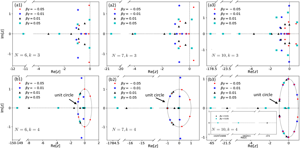
Figure 1: Distribution of Lee-Yang zeros for the nonlinearity $k=3$ in the case of (a1) $N=6$, (a2) $N=7$, and (a3) $N=10$ and for the nonlinearity $k=4$ in the case of (b1) $N=6$, (b2) $N=7$, and (b3) $N=10$. The red circles, blue pentagrams, black triangles, and cyan squares represent the Lee-Yang zeros for $\beta\gamma=-0.05$, $-0.01$, $0.01$, and $0.05$, respectively. The inset of (b3) shows the Lee-Yang zeros that are not presented in (b3).

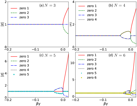
Figure 2: Norms of all Lee-Yang zeros in the case of $k=4$ for different spin numbers. The spin numbers are (a) $N=3$, (b) $N=4$, (c) $N=5$, and (d) $N=6$. Zero 1 to zero 6 in the plots are the labels of the Lee-Yang zeros.

Theorem 1. For the Hamiltonian (3), the point $(-1,0)$ in the complex plane is always a Lee-Yang zero when the spin number $N$ is odd and the nonlinearity $k$ is even.

This theorem can be proved by noticing that

$$\sum_{n=0}^{N}\binom{N}{n}e^{-\beta\gamma\left(n-\frac{N}{2}\right)^{k}}(-1)^{n}$$

$$= \sum_{n=0}^{\frac{N-1}{2}}\binom{N}{n}\!\!\left[e^{-\beta\gamma\left(n-\frac{N}{2}\right)^{k}}(-1)^{n}\!+\!e^{-\beta\gamma\left(\frac{N}{2}-n\right)^{k}}(-1)^{N-n}\right]\!,$$

where the equality $\binom{N}{n}=\binom{N}{N-n}$ was applied. In the case that $k$ is even, the equation above further reduces to

$$\sum_{n=0}^{\frac{N-1}{2}}\binom{N}{n}e^{-\beta\gamma\left(n-\frac{N}{2}\right)^{k}}\left[(-1)^{n}+(-1)^{N-n}\right]$$ (6)

When $N$ is odd, $(-1)^{n}+(-1)^{N-n}$ is always zero. The theorem is then proved. $\hfill\blacksquare$

In the case of $k=2$, all Lee-Yang zeros will be on the unit circle as long as $\beta\gamma$ is negative Wei2012 ; Peng2015 . However, as shown in Fig. 1, the situation becomes complex when $k$ is larger than $2$. In the case that $k$ is odd, we have the following theorem.

Theorem 2. For the Hamiltonian (3), the Lee-Yang zeros are never all distributed on the unit circle when the nonlinearity $k$ is odd.

According to Vieta’s formulas, the Lee-Yang zeros $\{z_{i}\}$ satisfy

$$\prod^{N}_{i=1}z_{i}=(-1)^{N}e^{\beta\gamma\left[\left(\frac{N}{2}\right)^{k}-\left(-\frac{N}{2}\right)^{k}\right]}.$$ (7)

In the case that $k$ is odd, one can further have $\prod^{N}_{i=1}|z_{i}|=e^{2\beta\gamma\left(\frac{N}{2}\right)^{k}}$. It is obvious that $e^{2\beta\gamma\left(\frac{N}{2}\right)^{k}}$ cannot be 1 as long as $\beta\gamma\neq 0$, indicating that the Lee-Yang zeros cannot be all distributed on the unit circle when in this case. The theorem is then proved. $\hfill\blacksquare$

From the proof above, one can immediately obtain the following theorem for an even nonlinearity.

Theorem 3. For the Hamiltonian (3), the Lee-Yang zeros satisfy $\prod^{N}_{i=1}|z_{i}|=1$ when the nonlinearity $k$ is even.

This theorem does not lead to the result that all Lee-Yang zeros are distributed on the unit circle when $k$ is even, which is already exhibited in Fig. 1(b). In the case of $k=4$, we find an interesting phenomenon for $N=3,4,5,6$ that the norms of all Lee-Yang zeros are $1$, namely, all Lee-Yang zeros are distributed on the unit circle, when $\beta\gamma$ is smaller than a critical value, as shown in Figs. 2(a) to 2(d) for $N=3$, $N=4$, $N=5$, and $N=6$, respectively. As a matter of fact, when $k=4$, the Lee-Yang zeros will always be distributed on the unit circle as long as $\beta\gamma$ is small enough, regardless of the value of $N$. This is due to the fact that when $k=4$, the equation $Z(z)=0$ reduces to

$$\sum^{N}_{n=0}\binom{N}{n}e^{\beta\gamma\left[\frac{N^{4}}{16}-\left(n-\frac{N}{2}\right)^{4}\right]}z^{n}=0.$$ (8)

It is obvious that

$$\frac{N^{4}}{16}-\left(n-\frac{N}{2}\right)^{4}=\frac{N^{4}}{16}\left[1-\left(\frac{2n}{N}-1\right)^{4}\right]\geq 0$$ (9)

for $n\in[0,N]$ since $n/N\leq 1$. Hence, when $\beta\gamma$ is small enough, namely, $\beta\gamma$ is negative and its absolute value is large enough, $e^{\beta\gamma[\frac{N^{4}}{16}-(n-\frac{N}{2})^{4}]}\approx 0$ and the equation above approximates to

$$1+z^{N}=0,$$ (10)

which immediately gives $|z|=1$, indicating that the Lee-Yang zeros are distributed on the unit circle. As a matter of fact, this result can be extended to the case of all even values of nonlinearity. In this case, the equation $Z(z)=0$ reduces to

$$\sum^{N}_{n=0}\binom{N}{n}e^{\beta\gamma\left[\left(\frac{N}{2}\right)^{k}-\left(n-\frac{N}{2}\right)^{k}\right]}z^{n}=0,$$ (11)

where $\left(\frac{N}{2}\right)^{k}-\left(n-\frac{N}{2}\right)^{k}\geq 0$. Therefore, when $\beta\gamma$ is small enough, the equation above always approximates to $1+z^{N}=0$ and the Lee-Yang zeros are thus distributed on the unit circle. Hence, we have the following theorem.

Theorem 4. For the Hamiltonian (3), the Lee-Yang zeros are always distributed on the unit circle for an even nonlinearity $k$ as long as $\beta\gamma$ is small enough.

In Figs. 2(a) to 2(d), there exists a critical value of $\beta\gamma$ for all zeros to be simultaneously distributed on the unit circle. Whether this critical point exists in general and how to analytically obtain this critical point are not answered in the theorem above and still remain open questions that require further investigations.

III Detection of Lee-Yang zeros with single qubit

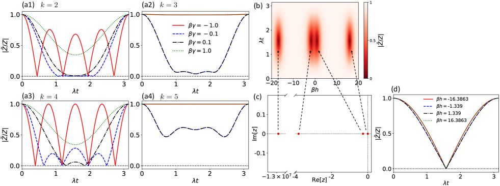
Figure 3: Detection of Lee-Yang zeros in the case of $N=4$. (a1)-(a4) The evolution of $|\tilde{Z}/Z|$ for (a1) $k=2$, (a2) $k=3$, (a3) $k=4$, and (a4) $k=5$. The solid red, dashed blue, dash-dotted black, and dotted green lines represent the values of amplitudes for $\beta\gamma=-1.0$, $-0.1$, $0.1$, and $1.0$, respectively. $\beta h$ is set to be zero in (a1)-(a4). (b) The values of $|\tilde{Z}/Z|$ as a function of $\beta h$ and $\lambda t$. (c) The distribution of Lee-Yang zeros. (d) The evolution of $|\tilde{Z}/Z|$ for the values of $\beta h$ to reach the Lee-Yang zeros. In (b)-(d) the nonlinearity $k=4$ and $\beta\gamma=1.0$.

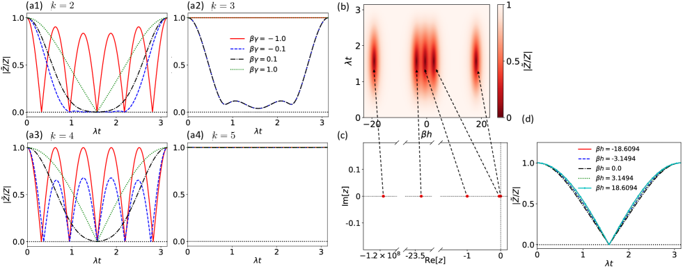
Figure 4: Detection of Lee-Yang zeros in the case of $N=5$. (a1)-(a4) The evolution of $|\tilde{Z}/Z|$ for (a1) $k=2$, (a2) $k=3$, (a3) $k=4$, and (a4) $k=5$. The solid red, dashed blue, dash-dotted black, and dotted green lines represent the values of amplitudes for $\beta\gamma=-1.0$, $-0.1$, $0.1$, and $1.0$, respectively. $\beta h$ is set to be zero in (a1)-(a4). (b) The values of $|\tilde{Z}/Z|$ as a function of $\beta h$ and $\lambda t$. (c) The distribution of Lee-Yang zeros. (d) The evolution of $|\tilde{Z}/Z|$ for the values of $\beta h$ to reach the Lee-Yang zeros. In (b)-(d) the nonlinearity $k=4$ and $\beta\gamma=0.5$.

The scheme of detecting Lee-Yang zeros with a probe qubit is first proposed by Wei and Liu in 2012 Wei2012 and was further simulated in experiments by Peng et al. in 2015 Peng2015 . Here we also consider the coupling between a probe state and Hamiltonian (3) and discuss the detection of Lee-Yang zeros. The total Hamiltonian is

$$H_{\mathrm{tot}}=H+\frac{1}{2}\omega_{0}\sigma_{z}+\lambda J_{z}\sigma_{z},$$ (12)

where $H$ is given in Eq. (3), $\omega_{0}$ is the frequency of the probe qubit, and $\lambda$ is the coupling strength between it and the nonlinear system. Now denote the total Hilbert space as $\mathcal{H}_{\mathrm{tot}}=\mathcal{H}_{\mathrm{q}}\otimes\mathcal{H}$ with $\mathcal{H}_{\mathrm{q}}$ and $\mathcal{H}$ the Hilbert space of the probe qubit and nonlinear system. In this way, $J_{z}$ here actually represents $\openone_{\mathrm{q}}\otimes J_{z}$, and $\sigma_{z}$ represents $(\ket{\uparrow}\bra{\uparrow}-\ket{\downarrow}\bra{\downarrow})\otimes\openone$ with $\openone_{\mathrm{q}}$ and $\openone$ the identity operators in $\mathcal{H}_{\mathrm{q}}$ and $\mathcal{H}$. Assume the initial state is a product state

$$\rho_{\mathrm{in}}=\rho_{0}\otimes\rho_{\mathrm{th}},$$ (13)

where $\rho_{0}$ is the initial state of the probe qubit and $\rho_{\mathrm{th}}=e^{-\beta H}/Z$ is the thermal state of the nonlinear system.

The evolved state $\rho_{t}$ for the probe qubit can be calculated via the equation

$$\rho_{t}=\mathrm{Tr}_{\mathcal{H}}\left(e^{-iH_{\mathrm{tot}}t}\rho_{\mathrm{in}}e^{iH_{\mathrm{tot}}t}\right),$$ (14)

where $\mathrm{Tr}_{\mathcal{H}}(\cdot)$ represents the partial trace on the nonlinear system. Utilizing this equation and realizing that

$$e^{-i\lambda tJ_{z}\sigma_{z}}=\cos(\lambda tJ_{z})\openone_{\mathrm{tot}}-i\sin(\lambda tJ_{z})\sigma_{z}$$ (15)

with $\openone_{\mathrm{tot}}$ the identity operator in $\mathcal{H}_{\mathrm{tot}}$, $\rho_{t}$ can be solved analytically. In the basis $\{\ket{\uparrow},\ket{\downarrow}\}$, $\rho_{t}$ can be expressed by

$$\rho_{t}=\left(\begin{array}[]{cc}[\rho_{0}]_{00}&\frac{\tilde{Z}}{Z}e^{-i\omega_{0}t}[\rho_{0}]_{01}\\ \frac{\tilde{Z}^{*}}{Z}e^{i\omega_{0}t}[\rho_{0}]_{10}&[\rho_{0}]_{11}\\ \end{array}\right),$$ (16)

where $[\rho_{0}]_{ij}$ is the $ij$th entry of $\rho_{0}$ and

$$\tilde{Z}=\mathrm{Tr}\left(e^{-\beta H-i2\lambda tJ_{z}}\right).$$ (17)

Similar to the partition function $Z$, $\tilde{Z}$ can also be expressed by

$$\tilde{Z}=e^{\left(\frac{1}{2}\beta h+i\lambda t\right)N}\sum_{n=0}^{N}\binom{N}{n}e^{-\beta\gamma\left(n-\frac{N}{2}\right)^{k}}\tilde{z}^{n}$$ (18)

with $\tilde{z}:=e^{-\beta h-i2\lambda t}$. Compared to Eq. (4), it is not difficult to see that the equations $Z(z)=0$ and $\tilde{Z}(\tilde{z})=0$ share the same solutions. Hence, $\tilde{Z}$ can also be factorized to

$$\tilde{Z}=e^{\left(\frac{1}{2}\beta h+i\lambda t\right)N-\beta\gamma\left(-\frac{N}{2}\right)^{k}}\prod_{i=1}^{N}\left(\tilde{z}-z_{i}\right).$$ (19)

As shown in Eq. (16), the nonlinear system is responsible for the evolution of the nondiagonal entries of $\rho_{t}$, indicating that the information of the Lee-Yang zeros $\{z_{i}\}$ is hidden in the dynamics of the probe qubit. Utilizing Eqs. (5) and (19), the amplitude $|\tilde{Z}e^{-i\omega_{0}t}/Z|=|\tilde{Z}/Z|$ reduces to

$$\left|\frac{\tilde{Z}}{Z}\right|=\left|\frac{\prod_{i=1}^{N}\left(\tilde{z}-z_{i}\right)}{\prod_{i=1}^{N}\left(z-z_{i}\right)}\right|.$$ (20)

From this expression, it can be seen that this amplitude above vanishes when $\tilde{z}$ reaches the zeros $\{z_{i}\}$. Hence, the zeros can be measured via the evolution of $|\tilde{Z}/Z|$ as long as it can vanish. The evolution of $|\tilde{Z}/Z|$ for different nonlinearity in the case of $\beta h=0$ is given in Figs. 3(a1) to 3(a4) [Figs. 4(a1) to 4(a4)] for $N=4$ ($N=5$). It can be seen that the Lee-Yang zeros can be easily detected via the amplitude $|\tilde{Z}/Z|$ when the nonlinearity $k$ is even, as shown in Figs. 3(a1) and 4(a1) for $k=2$ and Figs. 3(a3) and 4(a3) for $k=4$, especially when $\beta\gamma$ is negative. With the increase of $\beta\gamma$, it gets difficult for $|\tilde{Z}/Z|$ to vanish, indicating that the Lee-Yang zeros cannot be detected via the amplitude $|\tilde{Z}/Z|$ in this parameter region. In the case that $k$ is odd, as illustrated in Figs. 3(a2) and 4(a2) for $k=3$ and Figs. 3(a4) and 4(a4) for $k=5$, $|\tilde{Z}/Z|$ can hardly vanish, especially when the norm of $\beta\gamma$ is large. These phenomena indicate that some value regions of $\beta\gamma$ could be unfriendly for the detection of Lee-Yang zeros in this case. Then how to detect the Lee-Yang zeros in these regions of $\beta\gamma$ becomes a serious problem. Luckily, the distribution of Lee-Yang zeros $\{z_{i}\}^{N}_{i=1}$ does not rely on the values of $h$, yet the amplitude $|\tilde{Z}/Z|$ is dependent on it, which provides a method to further detect the Lee-Yang zeros in these cases.

We demonstrate this detection strategy for the nonlinearity $k=4$ in both cases of $N=4,\beta\gamma=1.0$ and $N=5,\beta\gamma=0.5$, as given in Figs. 3(b) to 3(d) and Figs. 4(b) to 4(d). From Fig. 3(b) [Fig. 4(b)], it can be seen that four vanishing points of $|\tilde{Z}/Z|$ are shown at the time $\lambda t=\pi/2$ when the values of $\beta h$ are changed from around $-20$ to $20$. These vanishing points correspond to the four Lee-Yang zeros in this case, as shown in Fig. 3(c) [Fig. 4(c)]. The reason why the zeros always occur at the time $\pi/2$ is due to the fact that all four Lee-Yang zeros are located on the negative axis of $\mathrm{Re}[z]$. To make sure $e^{-\beta h-i2\lambda t}$ is real and negative, the only available value of $\lambda t$ is $\lambda t=\pi/2$. In the meantime, in this case the proper values of $\beta h$ for the detection of Lee-Yang zeros are $\{-\ln|z_{i}|\}$, and the evolution of $|\tilde{Z}/Z|$ with $\beta h\in\{-\ln|z_{i}|\}$ are shown in Fig. 3(d) [Fig. 4(d)]. The vanishing points indeed always occur at the time $\pi/2$ and the Lee-Yang zeros are then detectable.

IV Quantum Fisher information matrix at the Lee-Yang zeros

Quantum Fisher information matrix is another important fundamental quantity in quantum mechanics and quantum information. In this section we discuss the behaviors of quantum Fisher information matrix of the probe qubit at the Lee-Yang zeros. For the evolved state in Eq. (16), the quantum Fisher information matrix for the parameters $\{\lambda,\beta\}$ can be calculated via the equation Dittmann1999 ; Liu2020

$$\mathcal{F}_{ab}=2\mathrm{Tr}\left[(\partial_{a}\rho_{t})(\partial_{b}\rho_{t})\right]$$ (21)

for a pure $\rho_{t}$, and

$$\mathcal{F}_{ab}= \leavevmode\nobreak\ \mathrm{Tr}\left[\left(\partial_{a}\rho_{t}\right)\left(\partial_{b}\rho_{t}\right)\right]$$

$$+\frac{1}{\det(\rho_{t})}\mathrm{Tr}\left[\rho_{t}\left(\partial_{a}\rho_{t}\right)\rho_{t}\left(\partial_{b}\rho_{t}\right)\right]$$ (22)

for a mixed $\rho_{t}$. The subscripts $a,b\in\{\lambda,\beta\}$. Next, denoting $g=\tilde{Z}/Z$, it can be seen that

$$\partial_{\lambda(\beta)}g=g\Delta E_{\lambda(\beta)}:=g(E_{\lambda(\beta)}-\tilde{E}_{\lambda(\beta)})$$ (23)

with $E_{\lambda(\beta)}=-\partial_{\lambda(\beta)}\ln Z$ and $\tilde{E}_{\lambda(\beta)}=-\partial_{\lambda(\beta)}\ln\tilde{Z}$. Here $E_{\beta}$ is nothing but the thermodynamic energy for the Hamiltonian (3). $E_{\lambda}=0$ due to the fact that $Z$ is independent of $\lambda$. Utilizing Eqs. (21) and (23), the entries of the quantum Fisher information matrix are of the form

$$\mathcal{F}_{\lambda\lambda(\beta\beta)}= \leavevmode\nobreak\ 4|g|^{2}|[\rho_{0}]_{01}|^{2}|\Delta E_{\lambda(\beta)}|^{2},$$ (24)

$$\mathcal{F}_{\lambda\beta}= \leavevmode\nobreak\ 4|g|^{2}|[\rho_{0}]_{01}|^{2}\mathrm{Re}\left[\Delta E_{\lambda}(\Delta E_{\beta})^{*}\right],$$ (25)

when $\rho_{t}$ is pure. And when $\rho_{t}$ is mixed, they are

$$\mathcal{F}_{\lambda\lambda(\beta\beta)}= \leavevmode\nobreak\ 4|g|^{2}|[\rho_{0}]_{01}|^{2}\Bigg{(}\left|\Delta E_{\lambda(\beta)}\right|^{2}$$

$$+\frac{|g|^{2}|[\rho_{0}]_{01}|^{2}\mathrm{Re}^{2}\left[\Delta E_{\lambda(\beta)}\right]}{[\rho_{0}]_{00}[\rho_{0}]_{11}-|g|^{2}|[\rho_{0}]_{01}|^{2}}\Bigg{)},$$ (26)

$$\mathcal{F}_{\lambda\beta}= \leavevmode\nobreak\ 4|g|^{2}|[\rho_{0}]_{01}|^{2}\Bigg{(}\mathrm{Re}\left[\Delta E_{\lambda}(\Delta E_{\beta})^{*}\right]$$

$$+\frac{|g|^{2}|[\rho_{0}]_{01}|^{2}\mathrm{Re}\left[\Delta E_{\lambda}\right]\mathrm{Re}\left[\Delta E_{\beta}\right]}{[\rho_{0}]_{00}[\rho_{0}]_{11}-|g|^{2}|[\rho_{0}]_{01}|^{2}}\Bigg{)}.$$ (27)

For the sake of investigating the general behaviors of the quantum Fisher information matrix at the Lee-Yang zeros, its general expression at these points should be provided. As a matter of fact, the value of $\tilde{Z}$ is zero when the zero of $g$ reaches a Lee-Yang zero. Taking $(\ket{\uparrow}+\ket{\downarrow})/\sqrt{2}$ as the initial state of the probe qubit and utilizing the condition $\tilde{Z}=0$, the entries of the quantum Fisher information matrix for both pure and mixed $\rho_{t}$ at the Lee-Yang zeros can be written as

$$\mathcal{F}_{\lambda\lambda(\beta\beta)} = \frac{1}{Z^{2}}\left|\partial_{\lambda(\beta)}\tilde{Z}\right|^{2},$$ (28)

$$\mathcal{F}_{\lambda\beta} = \frac{1}{Z^{2}}\mathrm{Re}\left[(\partial_{\lambda}\tilde{Z})(\partial_{\beta}\tilde{Z}^{*})\right].$$ (29)

Notice that the zero of $g$ can only reach one Lee-Yang zero with a group of specific values of $h$ and $\lambda$, which allows us to assume, without loss of generality, that Lee-Yang zero is $m$th zero ($z_{m}$), namely, $e^{-\beta h}\cos(2\lambda t)=\mathrm{Re}[z_{m}]$ and $e^{-\beta h}\sin(2\lambda t)=\mathrm{Im}[z_{m}]$. In the following we denote $h_{m}$ and $\lambda_{m}$ as the values of $h$ and $\lambda$ that satisfy these equations. In this case, $\partial_{\lambda}\tilde{Z}$ can be expressed by

$$\partial_{\lambda}\tilde{Z} = -i2te^{(\frac{1}{2}\beta h_{m}+i\lambda_{m}t)N-\beta\gamma\left(-\frac{N}{2}\right)^{k}}\prod_{i\neq m}(\tilde{z}-z_{i})z_{m},$$

$$\partial_{\beta}\tilde{Z} = -h_{m}e^{(\frac{1}{2}\beta h_{m}+i\lambda_{m}t)N-\beta\gamma\left(-\frac{N}{2}\right)^{k}}\prod_{i\neq m}(\tilde{z}-z_{i})z_{m}.$$

Hence, the entries of the quantum Fisher information matrix can be rewritten into

$$\mathcal{F}_{\lambda\lambda} = 4t^{2}e^{-2\beta h_{m}}\frac{\prod_{i\neq m}|(z_{m}-z_{i})|^{2}}{\prod^{N}_{i=1}(|z_{m}|-z_{i})^{2}},$$ (30)

$$\mathcal{F}_{\beta\beta} = h_{m}^{2}e^{-2\beta h_{m}}\frac{\prod_{i\neq m}|(z_{m}-z_{i})|^{2}}{\prod^{N}_{i=1}(|z_{m}|-z_{i})^{2}},$$ (31)

$$\mathcal{F}_{\lambda\beta} = 0.$$ (32)

From the perspective of quantum parameter estimation, $\mathcal{F}_{\lambda\beta}=0$ means that in theory, the optimal measurement can let the deviations of $\lambda$ and $\beta$ reach their precision limit simultaneously. Furthermore, when $z_{m}$ sits on the unit circle, $h$ has to be $0$ and $\mathcal{F}_{\beta\beta}$ vanishes. This result indicates that the probe qubit cannot work as the thermometer at the position of a Lee-Yang zero if this zero is on the unit circle.

Next, let us discuss a more specific regime that $\beta\gamma$ is small. Theorem 4 shows that in this regime the Lee-Yang zeros are always distributed on the unit circle for even nonlinearity. In this case, $Z$ and $\tilde{Z}$ can be approximated into

$$Z \approx 2e^{-\beta\gamma\left(\frac{N}{2}\right)^{k}}\cosh(\frac{1}{2}\beta hN),$$ (33)

$$\tilde{Z} \approx 2e^{-\beta\gamma\left(\frac{N}{2}\right)^{k}}\cosh(\frac{1}{2}\beta hN+i\lambda tN).$$ (34)

Utilizing Eqs. (33) and (34), $|g|^{2}$ can be written as

$$|g|^{2}=1-\frac{\sin^{2}(\lambda tN)}{\cosh^{2}\left(\frac{1}{2}\beta hN\right)}.$$ (35)

In the meantime, $\tilde{E}_{\lambda}$ and $\tilde{E}_{\beta}$ read

$$\tilde{E}_{\lambda} = tN\frac{\sin(2\lambda tN)-i\sinh(\beta hN)}{\cosh(\beta hN)+\cos(2\lambda tN)},$$ (36)

$$\tilde{E}_{\beta} = \!\gamma\left(\frac{N}{2}\right)^{k}\!\!-\frac{1}{2}hN\frac{\sinh(\beta hN)+i\sin(2\lambda tN)}{\cosh(\beta hN)+\cos(2\lambda tN)}.$$ (37)

Due to the fact that $E_{\lambda}=0$ and

$$E_{\beta}=\gamma\left(\frac{N}{2}\right)^{k}-\frac{1}{2}hN\tanh\left(\frac{1}{2}\beta hN\right),$$ (38)

one can immediately have

$$\Delta E_{\lambda} = -tN\frac{\sin(2\lambda tN)-i\sinh(\beta hN)}{\cosh(\beta hN)+\cos(2\lambda tN)},$$

$$\Delta E_{\beta} = \frac{1}{2}hN\frac{2\sin^{2}(\lambda tN)\tanh\left(\frac{1}{2}\beta hN\right)+i\sin(2\lambda tN)}{\cosh(\beta hN)+\cos(2\lambda tN)}.$$

Still taking the initial state of the probe qubit as $(\ket{\uparrow}+\ket{\downarrow})/\sqrt{2}$, the entries of the quantum Fisher information matrix for a pure $\rho_{t}$ [Eqs. (24) and (25)] can be expressed by

$$\mathcal{F}_{\lambda\lambda} = t^{2}N^{2}\left[1-\frac{\cos^{2}(\lambda tN)}{\cosh^{2}(\frac{1}{2}\beta hN)}\right],$$ (39)

$$\mathcal{F}_{\beta\beta} = \frac{1}{4}h^{2}N^{2}\frac{\sin^{2}(\lambda tN)}{\cosh^{4}(\frac{1}{2}\beta hN)},$$ (40)

$$\mathcal{F}_{\lambda\beta} = \frac{1}{2}htN^{2}\frac{\sin(2\lambda tN)\sinh(\beta hN)}{[1+\cosh(\beta hN)]^{2}}.$$ (41)

It is obvious that $\rho_{t}$ can only be pure when $|g|^{2}=1$, i.e., $\sin(\lambda tN)=0$, which means the expression of the quantum Fisher information matrix for pure states is only valid for some specific time points. And these points may not correspond to the Lee-Yang zeros. Hence, in the following we only discuss the case that $\rho_{t}$ is mixed. For a mixed $\rho_{t}$, the entries [Eqs. (26) and (27)] read

$$\mathcal{F}_{\lambda\lambda} = t^{2}N^{2},$$ (42)

$$\mathcal{F}_{\beta\beta} = \frac{1}{4}h^{2}N^{2}\frac{\sin^{2}(\lambda tN)}{\cosh^{2}\left(\frac{1}{2}\beta hN\right)},$$ (43)

$$\mathcal{F}_{\lambda\beta} = 0.$$ (44)

The fact that both $\mathcal{F}_{\lambda\lambda}$ and $\mathcal{F}_{\beta\beta}$ are proportional to $N^{2}$ indicates that although the evolved state is mixed, both the deviations of $\lambda$ and $\beta$ can beat the standard quantum limit, $1/\sqrt{N}$ in this case, and reach the scale of $1/N$. Standard quantum limit is an important precision limit and error scaling in quantum metrology. It usually represents the measurement capability of a classical apparatus, and beating it indicates that the estimations of $\lambda$ and $\beta$ with this nonlinear system would overperform, at least theoretically, many classical measurement apparatuses.

Different from the behaviors of $g$, the dynamics of $\mathcal{F}_{\lambda\lambda}$ does not show any relevance with the Lee-Yang zeros since it does not rely on the values of $\lambda$ and $h$. When the zero of $g$ reaches a Lee-Yang zero, the value of $\mathcal{F}_{\lambda\lambda}$ has no difference from other points. With respect to $\mathcal{F}_{\beta\beta}$, the phenomenon is the same as the aforementioned general discussion. In this case, the probe qubit cannot work as a thermometer at any Lee-Yang zero since all zeros are distributed on the unit circle, as stated in Theorem 4.

Although the probe qubit cannot be a thermometer at the Lee-Yang zeros, the direction of the zeros may still benefit the estimation of $\beta$. For example, Theorem 1 tells us that the point $(-1,0)$ is always a Lee-Yang zero in this case as long as $N$ is odd. On the direction of $(-1,0)$, the value of $\lambda t$ is $\pi/2+m\pi$ with $m$ a natural number. It is obvious that for these values $\sin^{2}(\lambda tN)$ is $1$ since $N$ is odd, and $\mathcal{F}_{\beta\beta}$ reach its maximum value with respect to the time.

V Conclusion

In summary, in this paper we proposed a nonlinear quantum spin model and discussed the distribution of the Lee-Yang zeros in this model. Four observations are provided. For an odd nonlinearity, not all the Lee-Yang zeros can be distributed on the unit circle simultaneously. In the case of an even nonlinearity, the point $(-1,0)$ is always a Lee-Yang zero when the spin number is odd. In the meantime, the production of the norms of all Lee-Yang zeros is always 1, and when $\beta\gamma$ is small enough, all Lee-Yang zeros will always be distributed on the unit circle. Furthermore, the detection of these Lee-Yang zeros via a probe qubit is thoroughly discussed. In the case that the amplitude $|\tilde{Z}/Z|$ has no zero point during the dynamics, a detection scheme has been proposed via tuning the parameters $h$ and $\lambda$. Moreover, the quantum Fisher information matrix for $\lambda$ and $\beta$ at the Lee-Yang zeros are calculated, including a specific regime that $\beta\gamma$ is very small, and the result reveals an interesting phenomenon that both parameters can reach their theoretical precision limit at the Lee-Yang zeros, and the probe qubit cannot work as a thermometer at a Lee-Yang zero if it sits on the unit circle.

Apart from the Lee-Yang zeros and quantum Fisher information matrix, many other properties of the proposed nonlinear model are also worth studying, such as the existence of phase transitions or symmetries, and their connections with Lee-Yang zeros, the potential physical realizations of this model, and the generation and storage of spin squeezing with it. We believe that the further investigations of this model would help the community better understand the roles of nonlinearity in quantum spin models and its effect and potential usage in quantum information science, especially in quantum metrology.

- (1) C. N. Yang and T. D. Lee, Statistical Theory of Equations of State and Phase Transitions. I. Theory of Condensation, Phys. Rev. 87, 404 (1952).
- (2) T. D. Lee and C. N. Yang, Statistical Theory of Equations of State and Phase Transitions. II. Lattice Gas and Ising Model, Phys. Rev. 87, 410 (1952).
- (3) B. Simon and R. B. Griffiths, The field theory as a classical Ising model, Commun. Math. Phys. 33, 145-164 (1973).
- (4) M. Kardar, Statistical Physics of Fields, (Cambridge University Press, Cambridge, 2007).
- (5) M. E. Fisher, Yang-Lee Edge Singularity and Field Theory, Phys. Rev. Lett. 40, 1610 (1978).
- (6) P. J. Kortman and R. B. Griffiths, Density of Zeros on the Lee-Yang Circle for Two Ising Ferromagnets, Phys. Rev. Lett. 27, 1439 (1971).
- (7) M. Suzuki and M. E. Fisher, Zeros of the Partition Function for the Heisenberg, Ferroelectric, and General Ising Models, J. Math. Phys. 12, 235 (1971).
- (8) E. H. Lieb and A. D. Sokal, A General Lee-Yang Theorem for One-Component and Multicomponent Ferromagnets, Commun. Math. Phys. 80, 153-179 (1981).
- (9) J. L. Monroe, Restrictions on the phase diagrams for a large class of multisite interaction spin systems, J. Stat. Phys. 65, 445–452 (1991).
- (10) C. Binek, Density of Zeros on the Lee-Yang Circle Obtained from Magnetization Data of a Two-Dimensional Ising Ferromagnet, Phys. Rev. Lett. 81, 5644 (1998).
- (11) B.-B. Wei, S.-W. Chen, H.-C. Po, and R.-B. Liu, Phase transitions in the complex plane of physical parameters, Sci. Rep. 4, 5202 (2014).
- (12) S.-Y. Kim, Yang-Lee Zeros of the Antiferromagnetic Ising Model, Phys. Rev. Lett. 93, 130604 (2004).
- (13) P. Tong and X. Liu, Lee-Yang Zeros of Periodic and Quasiperiodic Anisotropic Chains in a Transverse Field, Phys. Rev. Lett. 97, 017201 (2006).
- (14) A. García-Saez and T.-C. Wei, Density of Yang-Lee zeros in the thermodynamic limit from tensor network methods, Phys. Rev. B 92, 125132 (2015).
- (15) J. L. Lebowitz, D. Ruelle, and E. R. Speer, Location of the Lee-Yang zeros and absence of phase transitions in some Ising spin systems, J. Math. Phys. 53, 095211 (2012).
- (16) J. Fröhlich and P. Rodriguez, Some applications of the Lee-Yang theorem, J. Math. Phys. 53, 095218 (2012).
- (17) T. Kist, J. L. Lado, and C. Flindt, Lee-Yang theory of criticality in interacting quantum many-body systems, Phys. Rev. Research 3, 033206 (2021).
- (18) P. F. Arndt, Yang-Lee Theory for a Nonequilibrium Phase Transition, Phys. Rev. Lett. 84, 814 (2000).
- (19) K. Brandner, V. F. Maisi, J. P. Pekola, J. P. Garrahan, and C. Flindt, Experimental Determination of Dynamical Lee-Yang Zeros, Phys. Rev. Lett. 118, 180601 (2017).
- (20) P. M. Vecsei, J. L. Lado, and C. Flindt, Lee-Yang theory of the two-dimensional quantum Ising model, Phys. Rev. B 106, 054402 (2022).
- (21) C. Flindt and J. P. Garrahan, Trajectory Phase Transitions, Lee-Yang Zeros, and High-Order Cumulants in Full Counting Statistics, Phys. Rev. Lett. 110, 050601 (2013).
- (22) A. Deger, K. Brandner, and C. Flindt, Lee-Yang zeros and large-deviation statistics of a molecular zipper, Phys. Rev. E 97, 012115 (2018).
- (23) A. Deger and C. Flindt, Determination of universal critical exponents using Lee-Yang theory, Phys. Rev. Research 1, 023004 (2019).
- (24) A. Deger, F. Brange, and C. Flindt, Lee-Yang theory, high cumulants, and large-deviation statistics of the magnetization in the Ising model, Phys. Rev. B 102, 174418 (2020).
- (25) H. Yoshida and K. Takahashi, Dynamical Lee-Yang zeros for continuous-time and discrete-time stochastic processes, Phys. Rev. E 105, 024133 (2022).
- (26) H. Nishimori and R. B. Griffiths, Structure and motion of the Lee-Yang zeros, J. Math. Phys. 24, 2637 (1983).
- (27) R. David, Characterization of Lee-Yang polynomials, Ann. Math. 171, 589-603 (2010).
- (28) Q. Hou, J. Jiang, and C. M. Newman, Motion of Lee-Yang Zeros, J. Stat. Phys. 190, 56 (2023).
- (29) B.-B. Wei and R.-B. Liu, Lee-Yang Zeros and Critical Times in Decoherence of a Probe Spin Coupled to a Bath, Phys. Rev. Lett. 109, 185701 (2012).
- (30) X. Peng, H. Zhou, B. Wei, J. Cui, J. Du, and R. Liu, Experimental Observation of Lee-Yang Zeros, Phys. Rev. Lett. 114, 010601 (2015).
- (31) A. R. Kuzmak and V. M. Tkachuk, Detecting the Lee-Yang zeros of a high-spin system by the evolution of probe spin, EPL 125, 10004 (2019).
- (32) Y. Su, H. Liang, and X. Wang, Spin squeezing and concurrence under Lee-Yang dephasing channels, Phys. Rev. A 102, 052423 (2020).
- (33) C. W. Helstrom, Quantum Detection and Estimation Theory (New York: Academic, 1976).
- (34) A. S. Holevo, Probabilistic and Statistical Aspects of Quantum Theory (Amsterdam: North-Holland, 1982).
- (35) J. Liu, H. Yuan, X.-M. Lu, and X. Wang, quantum Fisher information matrix and multiparameter estimation, J. Phys. A: Math. Theor. 53, 023001 (2020).
- (36) D. Šafránek, Simple expression for the quantum Fisher information matrix, Phys. Rev. A 97, 042322 (2018).
- (37) B.-B. Wei, Probing Yang-Lee edge singularity by central spin decoherence, New J. Phys. 19, 083009 (2017).
- (38) M. Kitagawa and M. Ueda, Squeezed spin states, Phys. Rev. A 47, 5138 (1993).
- (39) J. Ma, X. Wang, C. P. Sun, and F. Nori, Quantum spin squeezing, Phys. Rep. 509, 89-165 (2011).
- (40) G.-R. Jin, Y.-C. Liu, and W.-M. Liu, Spin squeezing in a generalized one-axis twisting model, New J. Phys. 11, 073049 (2009).
- (41) J Dittmann, Explicit formulae for the Bures metric, J. Phys. A: Math. Gen. 32, 2663 (1999).