First Results of Axion Dark Matter Search with DANCE

Abstract

Axions are one of the well-motivated candidates for dark matter, originally proposed to solve the strong CP problem in particle physics. Dark matter Axion search with riNg Cavity Experiment (DANCE) is a new experimental project to broadly search for axion dark matter in the mass range of $10^{-17}~{}$\mathrm{e}\mathrm{V}$<m_{a}<10^{-11}~{}$\mathrm{e}\mathrm{V}$$. We aim to detect the rotational oscillation of linearly polarized light caused by the axion-photon coupling with a bow-tie cavity. The first results of the prototype experiment, DANCE Act-1, are reported from a 24-hour observation. We found no evidence for axions and set 95% confidence level upper limit on the axion-photon coupling $g_{a\gamma\gamma}\lesssim$8\text{\times}{10}^{-4}\text{\,}\mathrm{G}\mathrm{e}\mathrm{V}^{-1}$$ in $10^{-14}~{}$\mathrm{e}\mathrm{V}$<m_{a}<10^{-13}~{}$\mathrm{e}\mathrm{V}$$. Although the bound did not exceed the current best limits, this optical cavity experiment is the first demonstration of polarization-based axion dark matter search without any external magnetic field.

I Introduction

Axions are hypothetical particles generated from a pseudo-scalar field originally proposed to solve the strong CP problem in quantum chromodynamics (QCD) [1]. This idea is generally called “QCD axion”. Moreover, string theory predicts a plenitude of axion-like particles (ALPs) [2]. QCD axions and ALPs are one of the well-motivated candidates for dark matter (DM) because of their small masses and tiny interactions with matter sectors, and could behave like a non-relativistic classical wave field in the history of the universe [3, 4, 5, 6]. Hereafter in this article, we collectively call them “axions”.

The conventional way of searching for axions is to detect a phenomenon where axions convert into photons under an external magnetic field and vice versa, known as the Primakoff effect [7, 8, 9]. Astronomical observations are useful to probe the axion-photon conversion in the (extra)galactic magnetic fields, but no strong evidence has been found [10, 11]. CERN Axion Solar Telescope (CAST) looked for axions thermally produced in the Sun with a strong dipole magnet and set the current limit on the axion-photon coupling [12]. Some new projects with toroidal coils probed a tiny oscillatory magnetic field caused by axion DM and achieved the competitive limits to CAST [13, 14].

Recently, new experimental approaches to search for axions were proposed that do not need any strong magnetic field but use optical cavities instead [15, 16, 17, 18, 19, 20, 21, 22, 23, 24]. These methods aim to detect the phase velocity difference between left- and right-handed circular polarizations caused by a small coupling between axions and photons [25, 26]. Laser interferometers are good at probing frequencies of $\lesssim$100\text{\,}\mathrm{k}\mathrm{H}\mathrm{z}$$ and thus they have a good sensitivity in the corresponding axion mass region of $m_{a}\lesssim 10^{-10}~{}$\mathrm{e}\mathrm{V}$$. A key point in these techniques is how to cancel the polarization flipping due to the reflection on mirrors in order to accentuate the axion effect. One suggestion is to use a Mach-Zehnder interferometer with two cavities and a polarizing beam splitter [15], and another would be to use a Michelson interferometer with quarter-wave plates inside two arm cavities [16]. The authors of Ref. [17] came up with an idea to use a bow-tie ring cavity: Dark matter Axion search with riNg Cavity Experiment (DANCE) [22, 23, 24]. A bow-tie cavity is used to enhance the axion signal without any optics inside the cavity, which prevents optical elements from lowering the finesse of the cavity. The methods of injecting linearly polarized beam and tuning mirror angles [18], and applying squeezed states of light [19] were also proposed to improve the sensitivity over a wide range of axion masses.

In this work, we demonstrated the prototype experiment, DANCE Act-1, and obtained the upper limit on the axion-photon coupling from a 24-hour observation. This optical cavity experiment is the first demonstration of polarization-based axion DM search without any external magnetic field. This article is organized as follows. Section II gives a brief summary of the rotational oscillation of optical linear polarization caused by axion DM and an expected sensitivity obtained by axion signal amplification using a bow-tie cavity. Section III reports the experimental setup, its performance, and data acquisition. In Section IV the data analysis and results are described. Section V discusses the causes of sensitivity degradation. Finally, we conclude this work in Section VI.

II Principle and sensitivity

In this section, we briefly revisit the dynamics of the axion field, calculate its oscillation amplitude, and derive the sensitivity of our experiment to the axion-photon coupling. We set the natural unit $\hbar=c=1$ unless otherwise noted.

Axions couple to photons through the Chern-Simons interaction,

$$\mathcal{L} \supset\frac{g_{a\gamma\gamma}}{4}a(t)F_{\mu\nu}\tilde{F}^{\mu\nu}$$

$$=g_{a\gamma\gamma}\dot{a}(t)\epsilon_{ijk}A_{i}\partial_{j}A_{k}+\mathrm{(total\,derivative)},$$ (1)

where dot denotes the time derivative, $g_{a\gamma\gamma}$ is the axion-photon coupling constant, $a(t)$ is the axion field value, $A_{\mu}$ is the vector potential, and $F_{\mu\nu}\equiv\partial_{\mu}A_{\nu}-\partial_{\nu}A_{\mu}$. $\tilde{F}^{\mu\nu}\equiv\epsilon^{\mu\nu\rho\sigma}F_{\rho\sigma}/2$ is its Hodge dual defined with the Levi-Civita antisymmetric tensor $\epsilon^{\mu\nu\rho\sigma}$. We impose the temporal gauge $A_{0}=0$ and the Coulomb gauge $\nabla\cdot\bm{A}=0$. Then the equation of motion can be written as

$$\ddot{A}_{i}-\nabla^{2}A_{i}+g_{a\gamma\gamma}\dot{a}(t)\epsilon_{ijk}\partial_{j}A_{k}=0.$$ (2)

We decompose $A_{i}$ into two circular polarization modes in the Fourier space

$$A_{i}(t,\bm{x})=\sum_{\alpha=\mathrm{L},\mathrm{R}}\int^{\infty}_{-\infty}\frac{\mathrm{d}^{3}k}{(2\pi)^{3}}A_{\alpha}(t,\bm{k})e_{\alpha,i}(\hat{\bm{k}})e^{i\bm{k}\cdot\bm{x}},$$ (3)

where the index $\alpha$ of $\mathrm{L},\mathrm{R}$ represents left- and right-handed photons, $\bm{k}$ is the wave number vector, and $e_{\alpha,i}(\hat{\bm{k}})$ is the circular polarization vector. By substituting Eq. (3) into Eq. (2), we obtain the angular frequencies

$$\omega^{2}_{\mathrm{L}/\mathrm{R}}=k^{2}\quantity(1\mp\frac{g_{a\gamma\gamma}\dot{a}(t)}{k})$$ (4)

and the phase velocities

$$c_{\mathrm{L}/\mathrm{R}}\equiv\frac{\omega_{\mathrm{L}/\mathrm{R}}}{k}\simeq 1\mp\frac{g_{a\gamma\gamma}\dot{a}(t)}{2k}.$$ (5)

The axion field is expressed by a periodic oscillation,

$$a(t)=a_{0}\cos(m_{a}t+\delta_{\tau}(t)),$$ (6)

where the axion mass $m_{a}$ represents the angular frequency. The frequency of axion mass can be written as $f_{a}=m_{a}/(2\pi)\simeq$2.4\text{\,}\mathrm{H}\mathrm{z}$\,(m_{a}/10^{-14}~{}$\mathrm{e}\mathrm{V}$)$. The phase factor $\delta_{\tau}(t)$ can be regarded as a constant value within the constant timescale of axion DM, $\tau$, expressed as $\tau=2\pi/(m_{a}v^{2}_{a})$, where $v_{a}\sim 10^{-3}$ is the DM velocity near the Sun. Plugging Eq. (6) into Eq. (5), we obtain

$$c_{\mathrm{L}/\mathrm{R}} =1\pm\delta c(t),$$ (7)

$$\delta c(t) \equiv\frac{g_{a\gamma\gamma}\sqrt{2\rho_{a}}}{2k}\sin(m_{a}t+\delta_{\tau}(t)),$$ (8)

where $\rho_{a}=m_{a}^{2}a_{0}^{2}/2=$0.4\text{\,}\mathrm{G}\mathrm{e}\mathrm{V}\mathrm{/}\mathrm{c}\mathrm{m}^{3}$$ is the DM energy density in the Sun.

This phase velocity difference causes linearly polarized light to rotate [25, 26]. Let $\bm{E}(z=0,t)=E_{0}e^{i\omega_{0}t}\bm{e}_{\mathrm{s}}$ defined as the s-polarized injection beam propagating along the $z$ axis with angular frequency $\omega_{0}$ from $z=0$. The electric field at $z=l$ can be written as

$$\bm{E}(z=l,t)=E_{0}e^{i\omega t}(\bm{e}_{\mathrm{s}}\,\bm{e}_{\mathrm{p}})\matrixquantity(1\\ -\delta\theta(l,t)),$$ (9)

$$\delta\theta(l,t)\equiv k_{0}\int^{t}_{t-l}\delta c(t)\mathrm{d}t$$

$$=\frac{g_{a\gamma\gamma}\sqrt{2\rho_{a}}}{m_{a}}\sin(m_{a}\quantity(t-\frac{l}{2})+\delta_{\tau})\sin(m_{a}\frac{l}{2}),$$ (10)

when assuming $\delta\theta(l,t)\ll 1$. Here $k_{0}=\omega_{0}/c$ is the wave number without axions. The plane of linearly polarized light at $z=0$ rotates by $-\delta\theta(l,t)$ at $z=l$. Small p-polarized sidebands are generated from s-polarized carrier beam, and vice versa, in the presence of axions [18].

The sensitivity of DANCE Act-1 can be calculated using a method described in Ref. [27]. We assume that s-polarized light is injected into a bow-tie ring cavity, with an electric field of $\bm{E}_{\mathrm{in}}(t)=E_{0}e^{i\omega_{0}t}\bm{e}_{\mathrm{s}}$. The schematic of an experimental setup for DANCE Act-1 is shown in Fig. 1 and the symbols of the parameters are summarized in Table 1. Under the assumption that mirrors do not have any optical losses, the electric field of transmitted light is estimated as

$$\bm{E}_{\mathrm{trans}}(t)= \frac{\quantity(1-r_{1\mathrm{s}}^{2})e^{-ik_{0}l_{1}}}{\quantity(1-r_{1\mathrm{s}}^{2}r_{2\mathrm{s}}^{2})e^{-ik_{0}(2l_{1}+2l_{2})}}$$

$$\times E_{0}e^{i\omega_{0}t}(\bm{e}_{\mathrm{s}}\,\bm{e}_{\mathrm{p}})\matrixquantity(1\\ -\delta\phi(t)),$$ (11)

$$\delta\phi(t)\equiv \int_{-\infty}^{\infty}\frac{\mathrm{d}\omega}{2\pi}\tilde{\delta c}(\omega)e^{i\omega t}H_{a}(\omega),$$ (12)

where $\delta\phi(t)$ is a polarization rotation angle of transmitted light. $H_{a}(\omega)$ is a transfer function from $\delta c(t)$ to $\delta\phi(t)$:

$$H_{a}(\omega)\equiv k_{0}\sqrt{\frac{1-|r_{1\mathrm{p}}|^{2}}{1-|r_{1\mathrm{s}}|^{2}}}\frac{1}{i\omega\quantity(1-r_{1\mathrm{p}}^{2}r_{2\mathrm{p}}^{2})e^{-i\omega(2l_{1}+2l_{2})}}$$

$$\times\left[\quantity(1-e^{-i\omega l_{2}})\right.\quantity(r_{1\mathrm{s}}r_{2\mathrm{s}}r_{1\mathrm{p}}r_{2\mathrm{p}}e^{-i\omega l_{1}}+r_{1\mathrm{p}}^{2}r_{2\mathrm{p}}^{2}e^{-i\omega(2l_{1}+l_{2})})$$

$$\left.-\quantity(1-e^{-i\omega l_{1}})\quantity(r_{1\mathrm{s}}r_{2\mathrm{s}}^{2}r_{1\mathrm{p}}+r_{1\mathrm{s}}r_{1\mathrm{p}}r_{2\mathrm{p}}^{2}e^{-i\omega(l_{1}+l_{2})})\right].$$ (13)

The optical path length can be effectively increased using an optical cavity and axion signal is accumulated in the cavity. We set the reflectivity of s-polarization, $r_{1\mathrm{s}}$ and $r_{2\mathrm{s}}$, as real numbers, whereas that of p-polarization, $r_{1\mathrm{p}}$ and $r_{2\mathrm{p}}$, are complex numbers and contain the information about the difference of the reflective phase shift between s- and p-polarizations. For example, $r_{1\mathrm{p}}=|r_{1\mathrm{p}}|\exp[-2\pi i(2l_{1}+2l_{2})\delta\nu_{1}/c]$ where $\delta\nu_{1}$ is the reflective phase difference converted to the free spectral range (FSR) of a bow-tie cavity. $c/(2l_{1}+2l_{2})$ represents the FSR and its value in DANCE Act-1 is $302\text{\,}\mathrm{M}\mathrm{H}\mathrm{z}$.

Fig. 2 represents the response function $|H_{a}(m_{a})|$. When $\delta\nu_{1}=\delta\nu_{2}=0$, the sensitivity in the low mass region ($m_{a}\lesssim 10^{-12}~{}$\mathrm{e}\mathrm{V}$$) will be the highest. When $\delta\nu_{1}\neq 0$ or $\delta\nu_{2}\neq 0$, the sensitivity in the low mass region will be lower. However, the sensitivity is enhanced at the mass corresponding to the total reflective phase difference between s- and p-polarizations $\delta\nu_{\mathrm{total}}$ since signal sideband is enhanced in a bow-tie cavity.

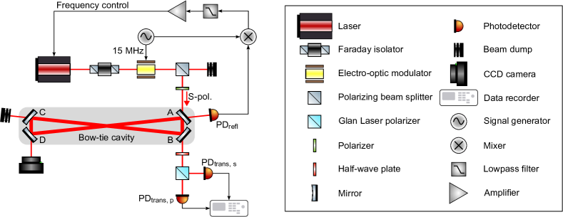
Figure 1: The schematic of an experimental setup for DANCE Act-1.

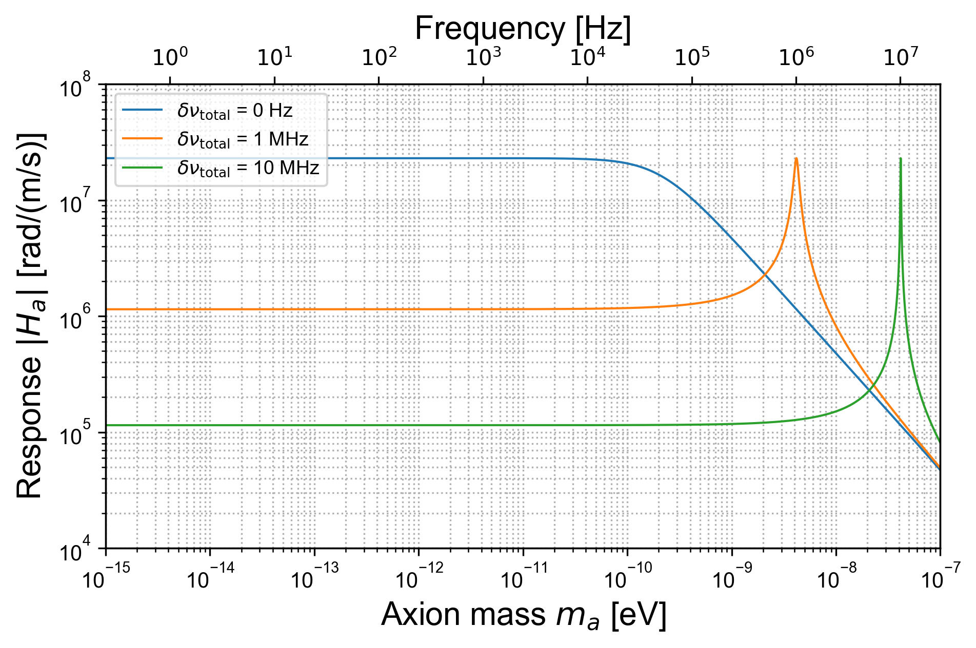
Figure 2: The response function $|H_{a}|$. The blue line shows the function $|H_{a}|$ for $\delta\nu_{1}=\delta\nu_{2}=$0\text{\,}\mathrm{H}\mathrm{z}$$ ($\delta\nu_{\mathrm{total}}=$0\text{\,}\mathrm{H}\mathrm{z}$$), the orange line for $\delta\nu_{1}=\delta\nu_{2}=$0.25\text{\,}\mathrm{M}\mathrm{H}\mathrm{z}$$ ($\delta\nu_{\mathrm{total}}=$1\text{\,}\mathrm{M}\mathrm{H}\mathrm{z}$$), and the green line for $\delta\nu_{1}=\delta\nu_{2}=$2.5\text{\,}\mathrm{M}\mathrm{H}\mathrm{z}$$ ($\delta\nu_{\mathrm{total}}=$10\text{\,}\mathrm{M}\mathrm{H}\mathrm{z}$$). The other parameters are the same as the final design of DANCE Act-1 as shown in Table 1.

The sensitivity of DANCE depends on the method of detection. The detailed setup of this work is described in Section III. The fundamental noise source of DANCE would be quantum shot noise and the potential sensitivity limited by shot noise is roughly estimated as

$$g_{a\gamma\gamma}\geq\left\{\begin{array}[]{l}$227\text{\,}\mathrm{G}\mathrm{e}\mathrm{V}^{-1}$\frac{\quantity|1-r_{1\mathrm{s}}^{2}r_{2\mathrm{s}}^{2}|}{\quantity|1-r_{1\mathrm{s}}^{2}|}\frac{$\mathrm{e}\mathrm{V}^{-1}$}{|H^{\prime}_{a}(m_{a})|/k_{0}}\\ \times\sqrt{\frac{$\mathrm{G}\mathrm{e}\mathrm{V}\mathrm{/}\mathrm{c}\mathrm{m}^{3}$}{\rho_{a}}\frac{$\mathrm{W}$}{P_{\mathrm{in}}}\frac{$\mathrm{\SIUnitSymbolMicro m}$}{\lambda_{0}}\frac{$\mathrm{s}$}{T_{\mathrm{obs}}}}\,\,\,\,\,(T_{\mathrm{obs}}\lesssim\tau),\\ $227\text{\,}\mathrm{G}\mathrm{e}\mathrm{V}^{-1}$\frac{\quantity|1-r_{1\mathrm{s}}^{2}r_{2\mathrm{s}}^{2}|}{\quantity|1-r_{1\mathrm{s}}^{2}|}\frac{$\mathrm{e}\mathrm{V}^{-1}$}{|H^{\prime}_{a}(m_{a})|/k_{0}}\\ \times\sqrt{\frac{$\mathrm{G}\mathrm{e}\mathrm{V}\mathrm{/}\mathrm{c}\mathrm{m}^{3}$}{\rho_{a}}\frac{$\mathrm{W}$}{P_{\mathrm{in}}}\frac{$\mathrm{\SIUnitSymbolMicro m}$}{\lambda_{0}}\frac{$\mathrm{s}$}{(T_{\mathrm{obs}}\tau)^{1/2}}}\,\,\,\,\,(T_{\mathrm{obs}}\gtrsim\tau),\end{array}\right.$$ (18)

$$|H^{\prime}_{a}(m_{a})|\equiv\frac{1}{2}\left\{(\operatorname{Re}\quantity[H_{a}(m_{a})+H_{a}(-m_{a})])^{2}\right.$$

$$\hskip 51.21495pt\left.+(\operatorname{Im}\quantity[H_{a}(m_{a})-H_{a}(-m_{a})])^{2}\right\}^{\frac{1}{2}},$$ (19)

where $\lambda_{0}$ is a laser wavelength and $|H^{\prime}_{a}(m_{a})|$ is a signal amplification factor by a bow-tie cavity. We assume that we can observe axions when ratio between axion signal and shot noise $\geq 1$. The sensitivity improves as the measurement time increases, with the factor of $T_{\mathrm{obs}}^{1/2}$ as long as the axion oscillation is coherent for $T_{\mathrm{obs}}\lesssim\tau$, where $\tau$ is the coherent timescale of axion DM. When the measurement time becomes longer than this coherence time $T_{\mathrm{obs}}\gtrsim\tau$, the proportionality of the sensitivity with the measurement time changes to $(T_{\mathrm{obs}}\tau)^{1/4}$. This different proportionality is owing to the stochasticity of the amplitude of axion field [28], which will be discussed in Section IV.

Even using conservative parameters listed in Table 1, DANCE Act-1 can exceed the CAST limit (see the green curve in Fig. 6). If we use more optimistic parameters, with a round-trip length of $10\text{\,}\mathrm{m}$, finesse of $10^{6}$, and input laser power of $100\text{\,}\mathrm{W}$, we can reach $g_{a\gamma\gamma}<$3\text{\times}{10}^{-16}\text{\,}\mathrm{G}\mathrm{e}\mathrm{V}^{-1}$$ for $m_{a}<10^{-16}~{}$\mathrm{e}\mathrm{V}$$ [17] and improve the sensitivity broadly by several orders of magnitude compared to the best upper limits at present.

Table 1: Summary of the parameters for DANCE Act-1. The difference of the reflective phase shift between s- and p-polarizations is written in the conversion to the FSR of the cavity ($\delta\nu=\mathrm{phase\,shift\,[rad]}/(2\pi)\times c/(2l_{1}+2l_{2})$). In the column for this experiment, the values with stars * are specifications, and the others are measured values. The parameters of the final design are listed to show the ideal sensitivity (plotted as the green curve in Fig. 6).

Parameter	Symbol	Final design	This experiment
Injected laser power	$P_{\mathrm{in}}$	$1\text{\,}\mathrm{W}$	$242(12)\text{\,}\mathrm{m}\mathrm{W}$
Transmitted laser power	$P_{\mathrm{trans}}$	$1\text{\,}\mathrm{W}$	$153(8)\text{\,}\mathrm{m}\mathrm{W}$
Distance between A and D, B and C	$l_{1}$	$45\text{\,}\mathrm{c}\mathrm{m}$	$45\text{\,}\mathrm{c}\mathrm{m}$ *
Distance between A and B, C and D	$l_{2}$	$4.7\text{\,}\mathrm{c}\mathrm{m}$	$4.7\text{\,}\mathrm{c}\mathrm{m}$ *
Power reflectivity of s-pol. (A and B)	$|r_{1\mathrm{s}}|^{2}$	99.9%	99.90(2)% *
Power reflectivity of s-pol. (C and D)	$|r_{2\mathrm{s}}|^{2}$	100%	$>$99.99% *
Power reflectivity of p-pol. (A and B)	$|r_{1\mathrm{p}}|^{2}$	99.9%	98.42(2)%
Power reflectivity of p-pol. (C and D)	$|r_{2\mathrm{p}}|^{2}$	100%	99.95(1)%
Finesse of s-pol. (carrier)	$\mathcal{F}_{\mathrm{s}}$	$3\text{\times}{10}^{3}$	$2.85(5)\text{\times}{10}^{3}$
Finesse of p-pol. (signal sidebands)	$\mathcal{F}_{\mathrm{p}}$	$3\text{\times}{10}^{3}$	195(3)
Total difference of the reflective phase shift between s- and p-pol.	$\delta\nu_{\mathrm{total}}$	$0\text{\,}\mathrm{H}\mathrm{z}$	$2.52(2)\text{\,}\mathrm{M}\mathrm{H}\mathrm{z}$
Difference of the reflective phase shift between s- and p-pol. (A and B)	$\delta\nu_{1}$	$0\text{\,}\mathrm{H}\mathrm{z}$	$-0.55(97)\text{\,}\mathrm{M}\mathrm{H}\mathrm{z}$
Difference of the reflective phase shift between s- and p-pol. (C and D)	$\delta\nu_{2}$	$0\text{\,}\mathrm{H}\mathrm{z}$	$2.08(99)\text{\,}\mathrm{M}\mathrm{H}\mathrm{z}$

III Experiment

In this section, the experimental setup, its performance and data acquisition are reported.

III.1 Setup and performance

Fig. 1 shows the experimental setup of DANCE Act-1. We used a Nd:YAG laser, Mephisto 500 NE, with a wavelength of 1064 nm. The s-polarized beam was injected into a bow-tie cavity. We put a polarizing beam splitter as well as a polarizer in front of the cavity to have linearly polarized light injected into the cavity. Our bow-tie cavity was constructed from four mirrors A-D rigidly fixed on a spacer made of aluminum.

We aim to probe the axion signal by taking the interference between a carrier beam (s-polarization in this work) and signal sidebands (p-polarization) in the direction of amplitude quadrature [18]. Polarization of transmitted light was rotated with a half-wave plate to introduce some p-polarized reference signal which has the same frequency as a carrier beam, and then split into s- and p-polarizations with a Glan Laser polarizer. The amplitudes of s- and p-polarizations were monitored with photodetectors PD_trans,s and PD_trans,p and saved with a data recorder for two weeks.

The laser frequency was locked to the resonance of TEM00 mode by obtaining the error signal for the laser frequency control with the Pound-Drever-Hall method [29]. Spatial mode is confirmed to be TEM00 using a CCD camera. To improve the lock duration time, the double-loop feedback control system and the automated cavity locking system were developed  [30]. Feedback signal above $\sim$30\text{\,}\mathrm{H}\mathrm{z}$$ was sent into the laser fast port (piezo actuator), and feedback signal under $\sim$30\text{\,}\mathrm{H}\mathrm{z}$$ was sent into the laser slow port (temperature actuator). To implement this system, we used SEAGULL mini as a digital signal processor, and also as a lowpass filter for the low frequency control loop. A digital signal processor monitored the output of PD_trans,s and identified whether the cavity was locked or unlocked. When the cavity was unlocked, signal into the laser slow port was swept until the cavity is locked again.

$l_{1}$ was designed to be around 10 times longer than $l_{2}$ to enhance the rotational oscillation of s-polarization by preventing the linear polarization from inverting when reflecting on mirrors. We specified only $|r_{1\mathrm{s}}|^{2}$ and $|r_{2\mathrm{s}}|^{2}$ when we ordered custom-made mirrors A-D because it is difficult to control the reflective phase shift and to satisfy our requirements. All the four mirrors were concave mirrors with a radius of curvature of $1\text{\,}\mathrm{m}$. Beam diameter on the mirrors was $\sim$800\text{\,}\mathrm{\SIUnitSymbolMicro}\mathrm{m}$$. Incident angles at all the four mirrors were $42\text{\,}\mathrm{d}\mathrm{e}\mathrm{g}$.

$\mathcal{F}_{\mathrm{s}}$, $\mathcal{F}_{\mathrm{p}}$, and $\delta\nu_{\mathrm{total}}$ were measured by sweeping cavity resonances. $\mathcal{F}_{\mathrm{s}}$ was consistent with the specified reflectivity $|r_{1\mathrm{s}}|^{2}$ and $|r_{2\mathrm{s}}|^{2}$ and we could achieve a high finesse. $\delta\nu_{\mathrm{total}}$ was non-zero because each polarization obtains a different phase shift from mirror-coating layers when reflecting at oblique incident angles. Note that $\delta\nu_{\mathrm{total}}$ drifted from $2.52(2)\text{\,}\mathrm{M}\mathrm{H}\mathrm{z}$ to $0.50(2)\text{\,}\mathrm{M}\mathrm{H}\mathrm{z}$ in the two-week observation. We obtained $\delta\nu_{1}$ and $\delta\nu_{2}$ separately for data analysis. We used mirrors with different coating layers to build the cavity and measured $\delta\nu_{\mathrm{total}}$ with various mirror combinations. Assuming that mirrors with the same coating layers have the same phase shift, we determined $\delta\nu_{1}$ and $\delta\nu_{2}$.

III.2 Data acquisition

The time series data of s- and p-polarizations, $P_{\mathrm{s}}(t)$ and $P_{\mathrm{p}}(t)$, was observed with a sampling rate of $1\text{\,}\mathrm{k}\mathrm{H}\mathrm{z}$ for 1,004,400 seconds in May 18-30, 2021. We analyzed two sets of continuous 86,400-second (24-hour) data on May 18 and 19 because the first two days were the stretch of time with the most stable lock. One set was used to set the upper limit and the other was used to veto candidate peaks.

We calibrated the output of photodetectors $P_{\mathrm{s}}(t)$ and $P_{\mathrm{p}}(t)$ to the rotation angle of linear polarization $\phi(t)$ by

$$\phi(t)=\sqrt{\frac{P_{\mathrm{p}}(t)}{P_{\mathrm{s}}(t)+P_{\mathrm{p}}(t)}}-2\theta_{\mathrm{HWP}},$$ (20)

where $\theta_{\mathrm{HWP}}$ is the rotation angle of the half-wave plate with respect to the s-polarized light at the detection port. We do not need to measure $\theta_{\mathrm{HWP}}$ because it is a constant parameter and we focus on oscillational amplitudes. The one-sided amplitude spectral density (ASD) of the observed rotation angle of linear polarization is plotted in Fig. 3. We reached $3.4\text{\times}{10}^{-6}\text{\,}\mathrm{r}\mathrm{a}\mathrm{d}\mathrm{/}\sqrt{Hz}$ at $5\text{\,}\mathrm{H}\mathrm{z}$.

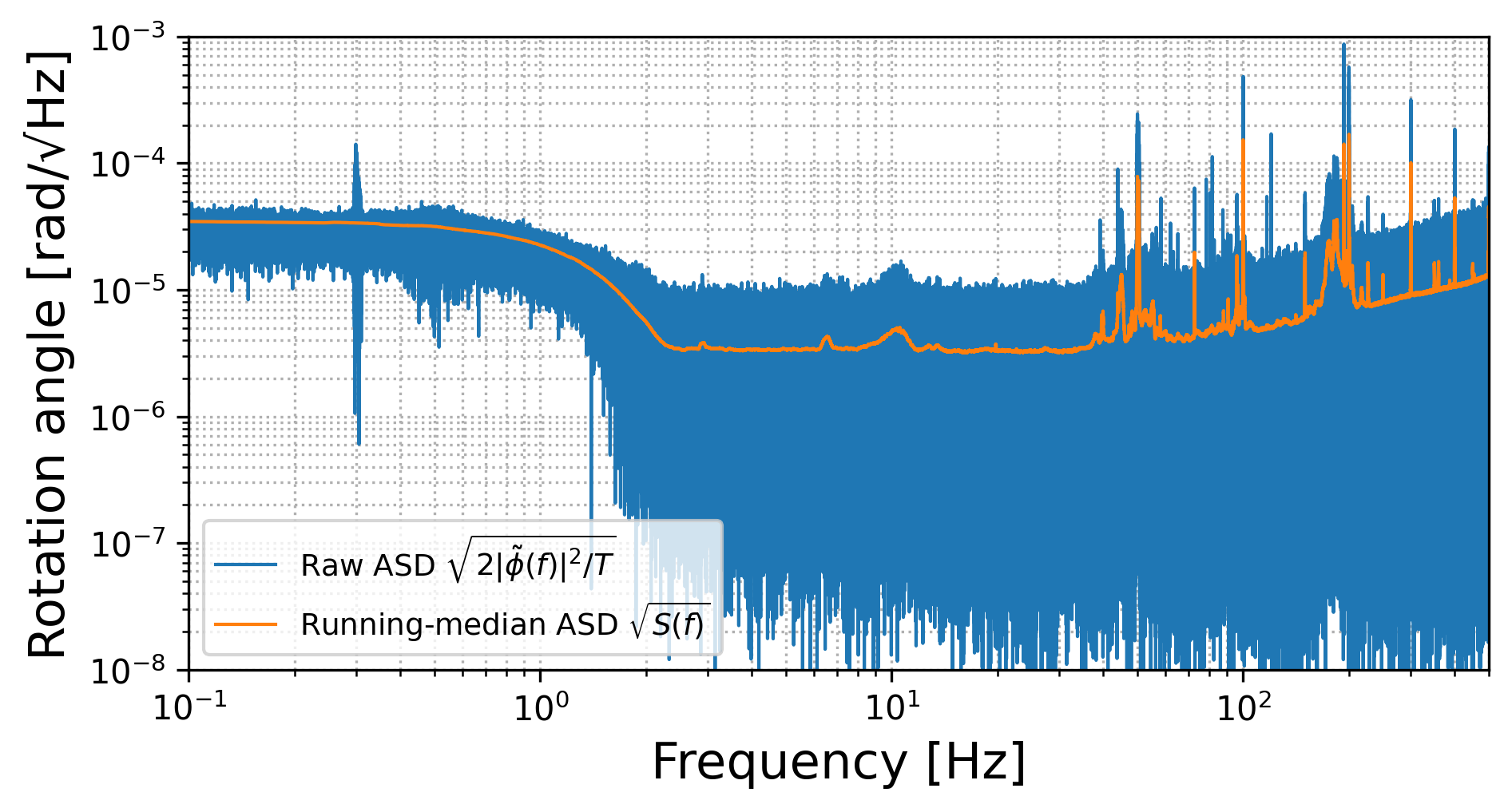
Figure 3: The one-sided ASD of the rotation angle of linear polarization.

IV Data analysis

In this section, we describe our analysis of the data to place upper limit on the axion-photon coupling.

IV.1 Detection statistics

The signal is expected to have a bandwidth of $\sim f_{a}v_{\mathrm{vir}}^{2}$, where $v_{\mathrm{vir}}$ is the virial velocity of our Galaxy [31]. Thus, for axion mass value $m_{a}$, we define the following signal-to-noise ratio (SNR) as a detection statistic:

$$\rho\equiv\sum_{f_{a}\leq f_{n}\leq f_{a}(1+\kappa^{2}v_{\mathrm{vir}}^{2})}\frac{4|\tilde{\phi}(f_{n})|^{2}}{TS(f_{n})},$$ (21)

where $T$ is the duration of the data segment, $f_{n}$ is the discretized frequency bin, $\kappa$ is a constant of order unity, $\tilde{\phi}(f)$ represents the Fourier-transformation of $\phi(t)$, and $S(f)$ is the one-sided noise power spectral density. Note that in the absence of the signal $\delta\phi(t)$, this corresponds to the orange curve in Fig. 3. Raw ASD is also plotted in Fig. 3. We adopt $v_{\mathrm{vir}}=$220\text{\,}\mathrm{k}\mathrm{m}\mathrm{/}\mathrm{s}$$ [32, 33], and $\kappa=3.17$ to guarantee that the fractional loss of signal is less than $99\%$ assuming the standard halo model of DM velocity distribution. Here $S(f_{n})$ is evaluated by the running median from $\sim 8,600$ neighboring frequency bins in order to smear out the effect of DM signal localized in the narrow band.

The detection threshold of $\rho$ is determined under the assumption that the instrumental noise is a stationary Gaussian process. In the absence of a signal, $\rho$ follows a $\chi^{2}$ distribution with $2N_{\mathrm{bin}}$ degrees of freedom, where $N_{\mathrm{bin}}$ denotes the number of frequency bins involved in the sum of Eq. (21). We chose the threshold to be the $95\%$ percentile of that distribution. For each case where the measured value of $\rho$ exceeds this threshold, we performed the veto analysis as explained below.

The upper bound on the signal amplitude is calculated in the frequentist method introduced by Ref. [28]. Because the axion field is superposition of particle waves with random phase, its amplitude randomly fluctuates. The analysis method proposed by the previous work takes into account this random axion amplitude. Let $\delta\phi^{\rm(upp)}(m_{a})$ denote the upper bound on the root-mean-square (RMS) of $\delta\phi(t)$ in Eq. (12) for axion mass value $m_{a}$. At the confidence level $\beta$, it is calculated by the following equation,

$$1-\beta=\int_{0}^{\rho_{\rm mea}(m_{a})}{\rm d}\rho~{}\mathcal{L}(\rho|\delta\phi^{\rm(upp)}(m_{a})),$$ (22)

where $\rho_{\rm mea}(m_{a})$ is the measured value of $\rho$, and $\mathcal{L}(\rho|\delta\phi)$ is the likelihood of observing detection statistics $\rho$ conditioned on signal with RMS $\delta\phi$. Note again that the effect of randomness in the axion DM amplitude mentioned above is included in the likelihood function derived in Ref. [28]. The interested readers can find the concrete expressions of this likelihood in Appendix. A. We chose $\beta=0.95$ for the numerical calculation of the upper bound. This upper bound on the rotation angle can be converted into that on the axion-photon coupling through the following relation:

$$g_{a\gamma\gamma}(m_{a})=\frac{2k_{0}\delta\phi^{\rm(upp)}(m_{a})}{\sqrt{2\rho_{a}}|H^{\prime}_{a}(m_{a})|}$$

$$=$5.10\text{\times}{10}^{11}\text{\,}\mathrm{G}\mathrm{e}\mathrm{V}^{-1}$\frac{$\mathrm{e}\mathrm{V}^{-1}$}{|H^{\prime}_{a}(m_{a})|/k_{0}}\sqrt{\frac{$\mathrm{G}\mathrm{e}\mathrm{V}\mathrm{/}\mathrm{c}\mathrm{m}^{3}$}{\rho_{a}}}\delta\phi^{\rm(upp)}(m_{a}).$$ (23)

IV.2 Results

After passing the first 24-hour data set through our pipeline for calculating $\rho_{\rm mea}(m_{a})$, 556 points exceeded the detection threshold of $\rho$ out of a total of 1,776,390 points in $0.1$-$490\text{\,}\mathrm{H}\mathrm{z}$ as shown in Fig. 4. We conducted the following two veto procedures: the persistence veto and the linewidth veto.

An axion signal should have the same frequency in two segments of data with the accuracy of $\Delta\omega/\omega\sim 10^{-6}$ [31]. We rejected the points that did not match the second set of data with 6 significant digits accuracy. This persistence veto reduced the number of candidate points to 257.

Since the expected linewidth of the galactic DM is $\Delta\omega/\omega\sim 10^{-6}$ [31], we eliminated the points that formed a peak wider than $10^{-5}$. The candidate points were decreased to 7 by this linewidth veto.

The frequencies of remaining peaks are summarized in Table 2. All the peaks were approximately multiples of $40\text{\,}\mathrm{H}\mathrm{z}$. As you can see in Fig. 5, peaks in the error signal of the laser frequency control had the same frequency as the peaks that were not rejected in the veto process. As the axion signal should not be present in the error signal, this suggests that the cause of remaining candidate peaks are from mechanical resonances of the cavity. We therefore rejected all the remaining candidate peaks.

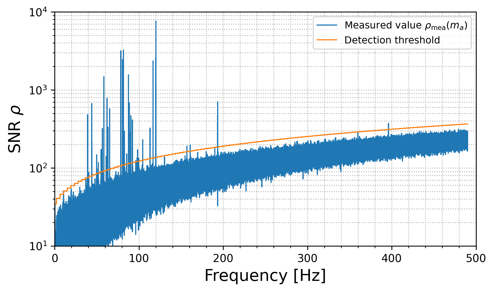
Figure 4: SNR $\rho$ of axion DM signal for each frequency $f_{a}$. The blue line shows the measured value $\rho_{\rm mea}(m_{a})$ and the orange line represents the detection threshold.

Table 2: Summary of remaining peaks after the veto procedures.

Frequency	SNR $\rho$ (Measured value)	SNR $\rho$ (Detection threshold)
$81.6712\text{\,}\mathrm{H}\mathrm{z}$	3243	109
$119.983\text{\,}\mathrm{H}\mathrm{z}$	2073	137
$120.001\text{\,}\mathrm{H}\mathrm{z}$	2616	137
$120.113\text{\,}\mathrm{H}\mathrm{z}$	1125	137
$120.117\text{\,}\mathrm{H}\mathrm{z}$	159	137
$120.118\text{\,}\mathrm{H}\mathrm{z}$	7637	137
$396.142\text{\,}\mathrm{H}\mathrm{z}$	373	313

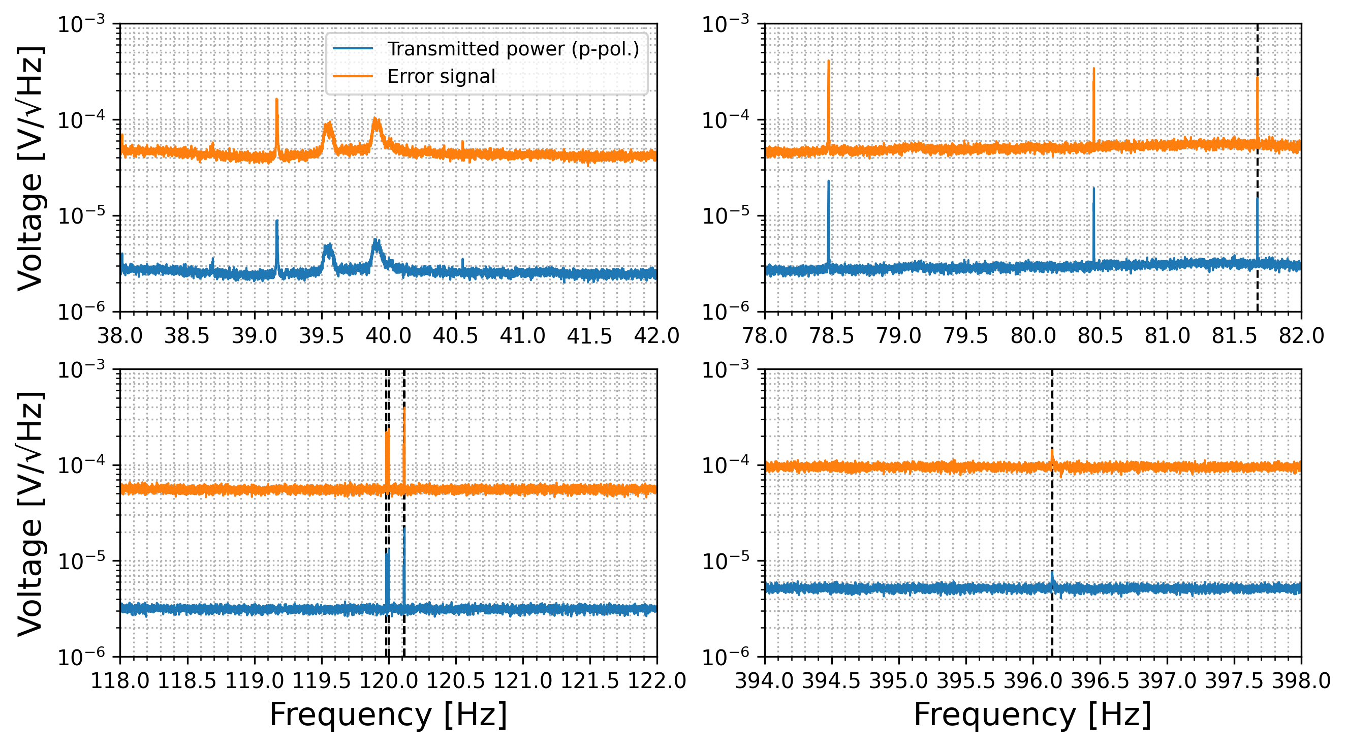
Figure 5: The one-sided amplitude spectral density of the transmitted p-polarization signal (blue line) and the error signal (orange line) around $40\text{\,}\mathrm{H}\mathrm{z}$ (upper left panel), $80\text{\,}\mathrm{H}\mathrm{z}$ (upper right panel), $120\text{\,}\mathrm{H}\mathrm{z}$ (lower left panel), and $400\text{\,}\mathrm{H}\mathrm{z}$ (lower right panel). Black dashed lines are the frequencies corresponding to the 7 remaining peaks summarized in Table 2.

We obtained the spectrum of the upper limit to the rotation angle of linearly polarized light $\delta\phi^{\rm(upp)}(m_{a})$ from the analysis pipeline, and calibrated it to the bound on the axion-photon coupling $g_{a\gamma\gamma}(m_{a})$ from Eq. (23). Note that the upper bound on the rotation angle of linear polarization $\delta\phi^{\rm(upp)}(m_{a})$ and the response function $|H^{\prime}_{a}|$ with the parameters of this work are plotted in Appendix A.

The initial value of $\delta\nu_{\mathrm{total}}=$2.52(2)\text{\,}\mathrm{M}\mathrm{H}\mathrm{z}$$ and the combination of $\delta\nu_{1}$ and $\delta\nu_{2}$ were found to be a major source of systematic effect, which will give 11% of difference in the upper limit at $m_{a}=10^{-13}\,{\rm eV}$. The values of these parameters were chosen to set the most conservative upper limit. The results are shown in Fig. 6. The upper limit was limited by classical noises and worse than the current shot noise by 5 orders of magnitude. Since $\delta\nu_{1}$ and $\delta\nu_{2}$ were non-zero, the current shot noise sensitivity was worse than the design sensitivity in the low mass range and has the dip at $m_{a}\simeq 10^{-8}~{}$\mathrm{e}\mathrm{V}$$ which corresponds to the frequency of $\delta\nu_{\mathrm{total}}$.

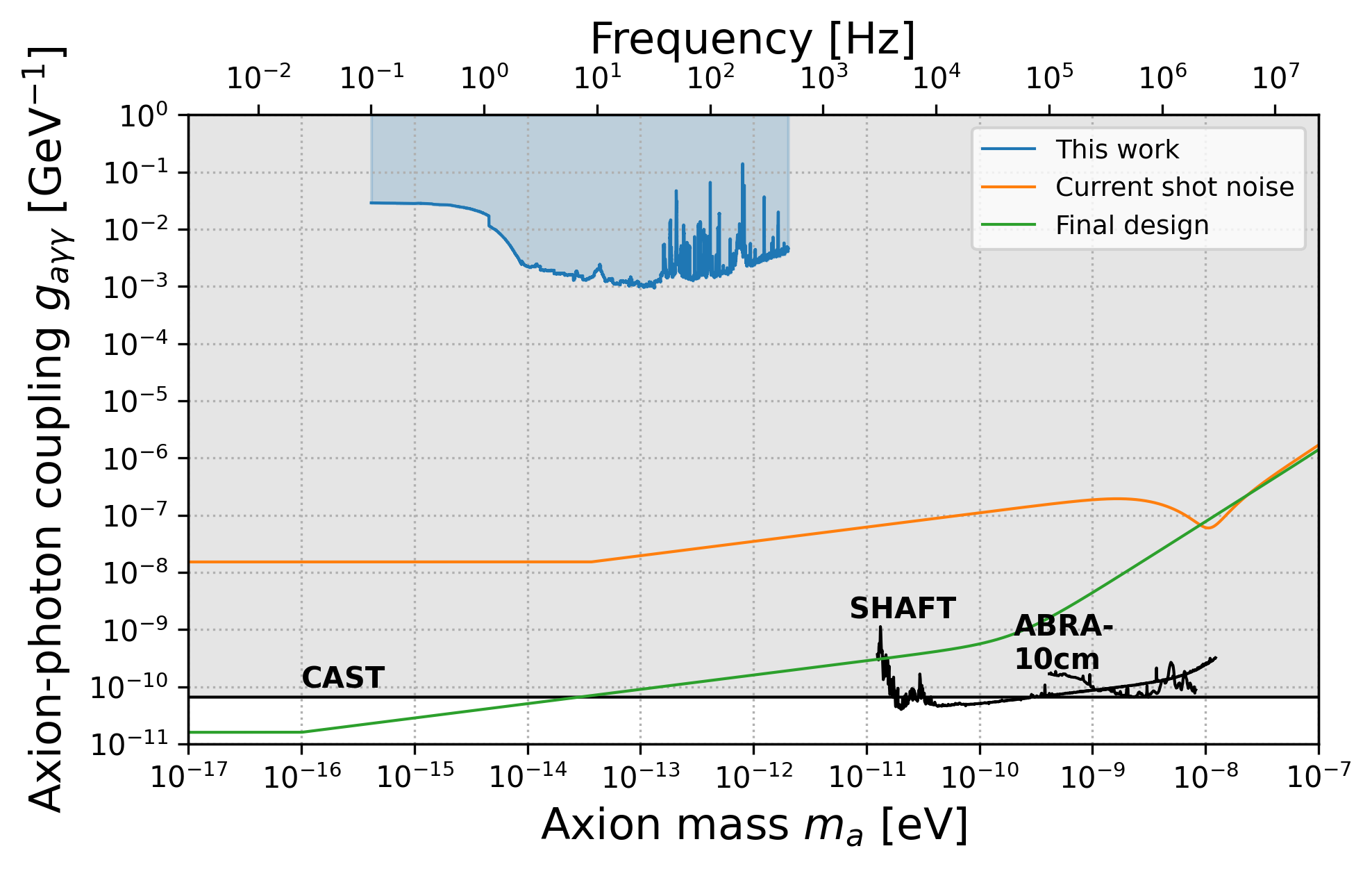
Figure 6: The blue line shows the upper limit on the axion-photon coupling constant obtained by this work. We observed for $T_{\mathrm{obs}}=$ 86,400 $\mathrm{s}\mathrm{e}\mathrm{c}\mathrm{o}\mathrm{n}\mathrm{d}\mathrm{s}$. The orange line is the expected sensitivity limited by shot noise with the same parameters as this work assuming $T_{\mathrm{obs}}=$ 86,400 $\mathrm{s}\mathrm{e}\mathrm{c}\mathrm{o}\mathrm{n}\mathrm{d}\mathrm{s}$. The green line represents the designed shot noise limited sensitivity of DANCE Act-1 assuming a observation time of $T_{\mathrm{obs}}=$1\text{\,}\mathrm{y}\mathrm{e}\mathrm{a}\mathrm{r}$$. The parameters which are used for this estimation are summarized in Table 1. The black lines with the grey-shaded region are current bounds obtained from CAST [12], SHAFT [13], and ABRACADABRA-10cm [14] experiments.

V Causes of sensitivity degradation

We discuss the two causes of sensitivity degradation in this experiment here. One is classical noise sources and the other is a non-zero phase difference between the two polarizations.

The rotation angle of linear polarization in $0.1$-$1\text{\,}\mathrm{H}\mathrm{z}$ correlated significantly with the injected laser power, and the rotation angle of linear polarization in $30\text{\,}\mathrm{H}\mathrm{z}$-$5\text{\,}\mathrm{k}\mathrm{H}\mathrm{z}$ correlated with the error signal for the frequency control. Thus, laser intensity noise, laser frequency noise, and mechanical vibration are some of the candidates for noise sources limiting our sensitivity. Furthermore, in principle the phase noises such as laser frequency noise and mechanical vibration are not supposed to contribute to noise for DANCE, which observes the signal in amplitude quadrature, but it could have coupled in this demonstration. The reduction of these noise sources is underway in our upgraded setup to be reported in future work.

The sensitivity is also reduced because of the reflective phase difference between two linear polarizations. If we can realize $\delta\nu_{1}=\delta\nu_{2}=0$, the sensitivity will improve by 3 orders of magnitude. We aim to deal with this issue by constructing an auxiliary cavity to achieve simultaneous resonance between both polarizations [19, 34].

VI Conclusion

The broadband axion DM search with a bow-tie cavity, DANCE Act-1 was demonstrated. We searched for the rotation and oscillation of linearly polarized light caused by the axion-photon coupling for 86,400 seconds and obtained the first results by DANCE. We found no evidence for axions and set 95% confidence level upper limit on the axion-photon coupling $g_{a\gamma\gamma}\lesssim$8\text{\times}{10}^{-4}\text{\,}\mathrm{G}\mathrm{e}\mathrm{V}^{-1}$$ in the axion mass range of $10^{-14}~{}$\mathrm{e}\mathrm{V}$<m_{a}<10^{-13}~{}$\mathrm{e}\mathrm{V}$$.

The candidates for noise sources limiting our sensitivity are laser intensity noise, frequency noise, and mechanical vibration. The sensitivity will be improved by introducing laser intensity control and a vibration isolation system as well as upgrading the frequency control system. The difference of reflective phase shift between s- and p-polarizations is also the cause for the sensitivity degradation. We are installing an auxiliary cavity to realize simultaneous resonance between the two polarizations [34].

Although the upper limit did not exceed the current best limits, this optical cavity experiment is the first demonstration of polarization-based axion dark matter search without any external magnetic field. By sufficiently upgrading the setup using the techniques mentioned above, we are expecting to improve the sensitivity by several orders of magnitude.

VII Acknowledgement

We would like to thank Shigemi Otsuka and Togo Shimozawa for manufacturing the mechanical parts, Kentaro Komori and Satoru Takano for fruitful discussions, and Ching Pin Ooi for editing this paper. This work is supported by JSPS KAKENHI Grant Nos. JP18K13537, JP20H05850, JP20H05854, and JP20H05859, by the Sumitomo Foundation, and by JST PRESTO Grant No. JPMJPR200B. Y. O. is supported by Grant-in-Aid for JSPS Fellows No. JP22J21087 and by JSR Fellowship, the University of Tokyo. H. F. is supported by Grant-in-Aid for JSPS Fellows No. JP22J21530 and by Forefront Physics and Mathematics Program to Drive Transformation (FoPM), a World-leading Innovative Graduate Study (WINGS) Program, the University of Tokyo. J. K. is supported by Grant-in-Aid for JSPS Fellows No. JP20J21866 and by research program of the Leading Graduate Course for Frontiers of Mathematical Sciences and Physics (FMSP). A. N. is supported by JSPS KAKENHI Grant Nos. JP19H01894 and JP20H04726 and by Research Grants from Inamori Foundation. I. O. is supported by JSPS KAKENHI Grant No. JP19K14702.

Appendix A Likelihood function of SNR and the upper limits

As shown in Ref. [28], the Fourier mode of signal with mass $m_{a}$ can be expressed in terms of the stochastic variables as

$$\delta\phi(f_{n};m_{a}) \simeq g_{a\gamma\gamma}(m_{a})\frac{\sqrt{2\rho_{a}}}{2k_{0}}|H^{\prime}_{a}(m_{a})|T$$ (24)

$$~{}~{}\times\sqrt{\Delta_{s}(f_{n};m_{a})}~{}\left[\frac{r_{n}}{{\sqrt{2}}}e^{i\theta_{n}}\right],$$

$$\equiv\delta\phi(m_{a})\frac{T}{2}\sqrt{\Delta_{s}(f_{n};m_{a})}\left[\frac{r_{n}}{{\sqrt{2}}}e^{i\theta_{n}}\right],$$ (25)

where $\theta_{n}$ and $r_{n}$ respectively obey a uniform distribution over $\left[0,2\pi\right]$ and the standard Rayleigh distribution. $\Delta_{s}(f_{n};m_{a})$ is the analytic function that represents the deterministic part of the spectral shape determined by the velocity distribution of DM (see Ref. [28] for details). By performing the marginalization over $r_{n}$, the likelihood that takes into account the random amplitude of DM signal can be obtained as

$$\mathcal{L}(\rho_{n}|\lambda_{n}) \equiv\int{\rm d}r_{n}~{}P_{R}(r_{n}){\mathcal{L}}\left(\rho_{n}\big{|}\lambda_{n}r_{n}\right)$$

$$=\frac{1}{{2}(1+\lambda_{n}^{2})}\exp\left(\frac{-\rho_{n}}{{2}(1+\lambda_{n}^{2})}\right),$$ (26)

where $\rho_{n}=4|\tilde{\phi}(f_{n})|^{2}/TS(f_{n})$ is the SNR at frequency bin $f_{n}$. As can be seen, the likelihood is characterized by the parameter

$$\lambda_{n}\equiv\delta\phi(m_{a})\sqrt{\Delta_{s}(f_{n};m_{a})}\sqrt{\frac{T}{2S(f_{n})}},$$ (27)

that depends on the characteristic amplitude of signal $\delta\phi(m_{a})$. Then from this expression, the likelihood for the (total) SNR $\rho=\Sigma_{n}\rho_{n}$ defined in Eq. (21) can be derived as

$$\mathcal{L}(\rho|\{\lambda_{n}\}) =\int\left(\prod_{l}^{N_{\mathrm{bin}}}{\rm d}\rho_{n}~{}\mathcal{L}(\rho_{n}|\lambda_{n})\right)\delta\left(\rho-\sum_{n}^{N_{\mathrm{bin}}}\rho_{n}\right)$$

$$=\sum_{n}^{N_{\mathrm{bin}}}\frac{w_{n}}{{2}(1+\lambda_{n}^{2})}\exp\left(-\frac{\rho}{{2}(1+\lambda_{n}^{2})}\right),$$ (28)

$$w_{n} \equiv\prod_{n^{\prime}(\neq n)}^{N_{\mathrm{bin}}}\frac{1+\lambda_{n}^{2}}{\lambda_{n}^{2}-\lambda_{n^{\prime}}^{2}},$$ (29)

where $\lambda_{n}\neq\lambda_{n^{\prime}}$ is assumed for all frequency bins $n\neq n^{\prime}$. We should note that this assumption would be violated and there arises a numerical instability, specifically for higher DM masses which involves more frequency bins in Eq. (21). In this case, however, we can use the Gaussian approximation of Eq. (28):

$${\mathcal{L}}(\rho|\{\lambda_{n}\}) \to\frac{1}{\sqrt{2\pi\sigma^{2}_{\rho}}}\exp\left(-\frac{(\rho-\mu_{\rho})^{2}}{2\sigma^{2}_{\rho}}\right)\quad\mathrm{for}\quad T\gg\tau,$$ (30)

$$\mu_{\rho} =2\sum_{n}(1+\lambda_{n}^{2}),$$ (31)

$$\sigma^{2}_{\rho} ={4}\sum_{n}(1+\lambda_{n}^{2})^{2}.$$ (32)

In our analysis, we apply this Gaussian approximation for $N_{\mathrm{bin}}>8$.

From these expressions of likelihood function, we could numerically set the 95% confidence limit on $\left\{\lambda_{n}\right\}$, or equivalently on $\delta\phi(m_{a})$ according to Eq. (22). The upper bound $\delta\phi^{\rm(upp)}(m_{a})$ derived in our pipeline is shown in Fig. 7. As mentioned in the main text, $\delta\phi^{\rm(upp)}(m_{a})$ is converted to the upper limit on $g_{a\gamma\gamma}$ with Eq. (23). This was achieved by using the response function $|H^{\prime}_{a}|$ presented in Fig. 8.

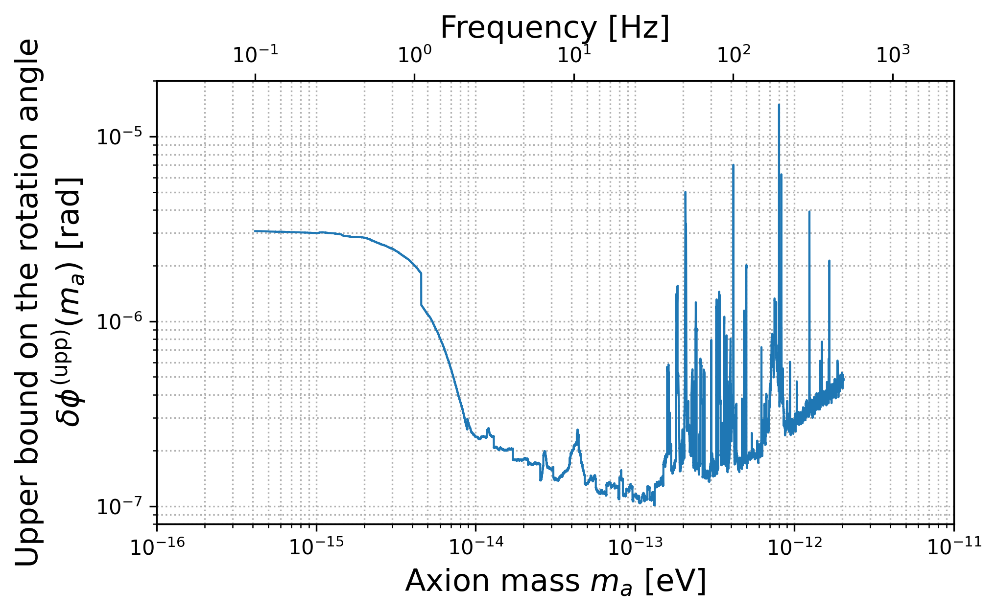
Figure 7: The upper bound on the rotation angle of linear polarization $\delta\phi^{\rm(upp)}(m_{a})$.

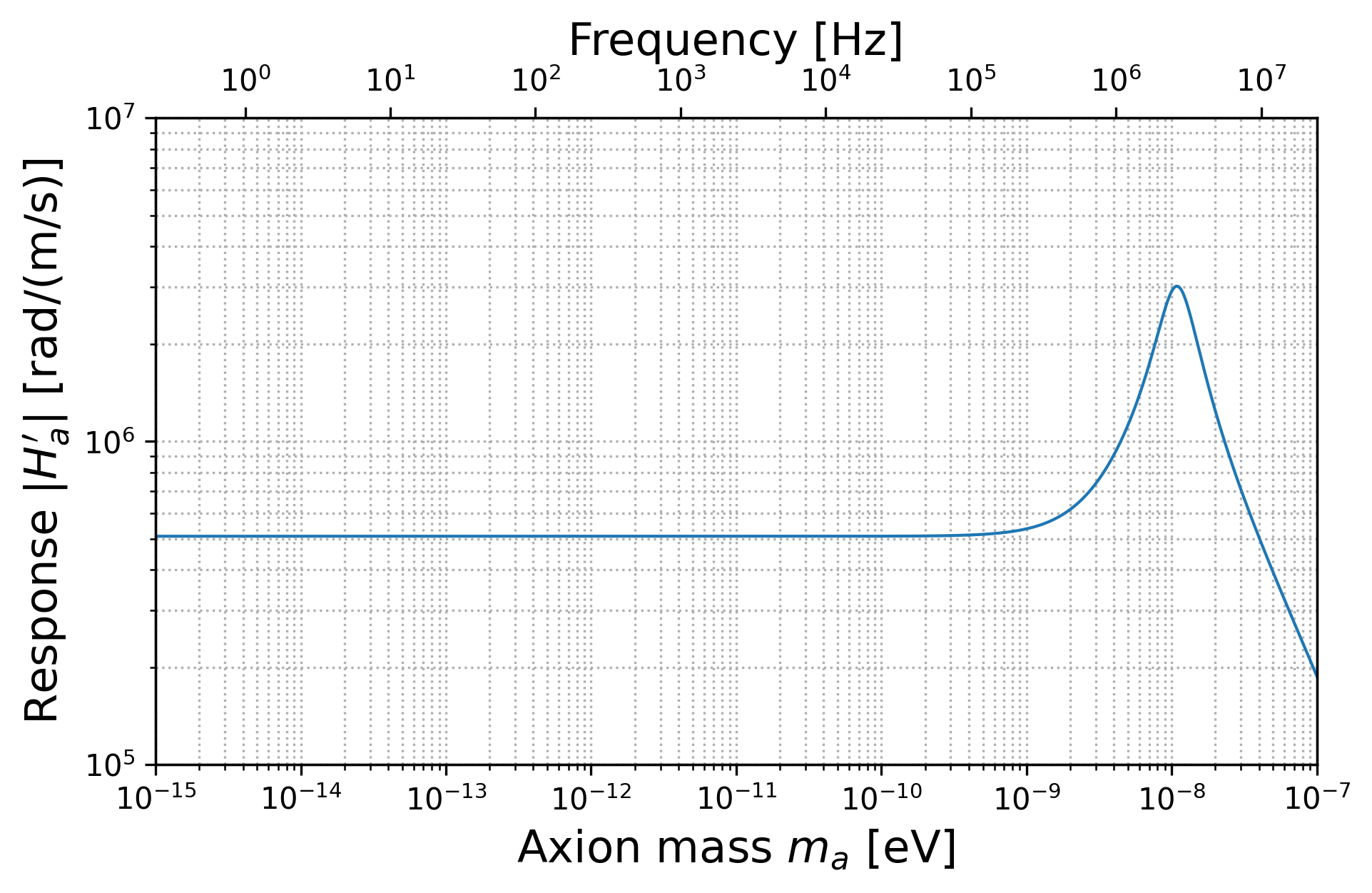
Figure 8: The response function with the parameters of this experiment $|H^{\prime}_{a}|$. The parameters were chosen from Table 1 to set the most conservative upper limit.

References

- Peccei and Quinn [1977] R. D. Peccei and H. R. Quinn, Phys. Rev. Lett. 38, 1440 (1977).
- Arvanitaki et al. [2010] A. Arvanitaki, S. Dimopoulos, S. Dubovsky, N. Kaloper, and J. March-Russell, Phys. Rev. D 81, 123530 (2010).
- Preskill et al. [1983] J. Preskill, M. B. Wise, and F. Wilczek, Physics Letters B 120, 127 (1983).
- Abbott and Sikivie [1983] L. Abbott and P. Sikivie, Physics Letters B 120, 133 (1983).
- Dine and Fischler [1983] M. Dine and W. Fischler, Physics Letters B 120, 137 (1983).
- Arias et al. [2012] P. Arias, D. Cadamuro, M. Goodsell, J. Jaeckel, J. Redondo, and A. Ringwald, Journal of Cosmology and Astroparticle Physics 2012 (06), 013.
- Sikivie [1983] P. Sikivie, Phys. Rev. Lett. 51, 1415 (1983).
- Schneider et al. [1984] M. B. Schneider, F. P. Calaprice, A. L. Hallin, D. W. MacArthur, and D. F. Schreiber, Phys. Rev. Lett. 52, 695 (1984).
- Raffelt and Stodolsky [1988] G. Raffelt and L. Stodolsky, Phys. Rev. D 37, 1237 (1988).
- Payez et al. [2015] A. Payez, C. Evoli, T. Fischer, M. Giannotti, A. Mirizzi, and A. Ringwald, Journal of Cosmology and Astroparticle Physics 2015 (02), 006.
- Reynolds et al. [2020] C. S. Reynolds, M. C. D. Marsh, H. R. Russell, A. C. Fabian, R. Smith, F. Tombesi, and S. Veilleux, The Astrophysical Journal 890, 59 (2020).
- Anastassopoulos et al. [2017] V. Anastassopoulos et al. (Collaboration, C. A. S. T.), Nature Physics 13, 584 (2017).
- Gramolin et al. [2021] A. V. Gramolin, D. Aybas, D. Johnson, J. Adam, and A. O. Sushkov, Nature Physics 17, 79 (2021).
- Salemi et al. [2021] C. P. Salemi, J. W. Foster, J. L. Ouellet, A. Gavin, K. M. W. Pappas, S. Cheng, K. A. Richardson, R. Henning, Y. Kahn, R. Nguyen, N. L. Rodd, B. R. Safdi, and L. Winslow, Phys. Rev. Lett. 127, 081801 (2021).
- Melissinos [2009] A. C. Melissinos, Phys. Rev. Lett. 102, 202001 (2009).
- DeRocco and Hook [2018] W. DeRocco and A. Hook, Phys. Rev. D 98, 035021 (2018).
- Obata et al. [2018] I. Obata, T. Fujita, and Y. Michimura, Phys. Rev. Lett. 121, 161301 (2018).
- Liu et al. [2019] H. Liu, B. D. Elwood, M. Evans, and J. Thaler, Phys. Rev. D 100, 023548 (2019).
- Martynov and Miao [2020] D. Martynov and H. Miao, Phys. Rev. D 101, 095034 (2020).
- Nagano et al. [2019] K. Nagano, T. Fujita, Y. Michimura, and I. Obata, Phys. Rev. Lett. 123, 111301 (2019).
- Nagano et al. [2021] K. Nagano, H. Nakatsuka, S. Morisaki, T. Fujita, Y. Michimura, and I. Obata, Phys. Rev. D 104, 062008 (2021).
- Michimura et al. [2020] Y. Michimura, Y. Oshima, T. Watanabe, T. Kawasaki, H. Takeda, M. Ando, K. Nagano, I. Obata, and T. Fujita, Journal of Physics: Conference Series 1468, 012032 (2020).
- Oshima et al. [2021a] Y. Oshima, H. Fujimoto, M. Ando, T. Fujita, Y. Michimura, K. Nagano, I. Obata, and T. Watanabe, Dark matter axion search with ring cavity experiment dance: Current sensitivity (2021a), arXiv:2105.06252 [hep-ph] .
- Oshima et al. [2021b] Y. Oshima, H. Fujimoto, M. Ando, T. Fujita, J. Kume, Y. Michimura, S. Morisaki, K. Nagano, H. Nakatsuka, A. Nishizawa, I. Obata, and T. Watanabe, Journal of Physics: Conference Series 2156, 012042 (2021b).
- Carroll et al. [1990] S. M. Carroll, G. B. Field, and R. Jackiw, Phys. Rev. D 41, 1231 (1990).
- Carroll [1998] S. M. Carroll, Phys. Rev. Lett. 81, 3067 (1998).
- [27] H. Fujimoto, Y. Oshima, J. Kume, S. Morisaki, K. Nagano, T. Fujita, I. Obata, A. Nishizawa, Y. Michimura, and M. Ando, in preparation.
- Nakatsuka et al. [2022] H. Nakatsuka, S. Morisaki, T. Fujita, J. Kume, Y. Michimura, K. Nagano, and I. Obata, Stochastic effects on observation of ultralight bosonic dark matter (2022), arXiv:2205.02960 [astro-ph.CO] .
- Drever et al. [1983] R. W. P. Drever, J. L. Hall, F. V. Kowalski, J. Hough, G. M. Ford, A. J. Munley, and H. Ward, Applied Physics B 31, 97 (1983).
- Fujimoto et al. [2021a] H. Fujimoto, Y. Oshima, M. Ando, T. Fujita, Y. Michimura, K. Nagano, and I. Obata, Dark matter axion search with ring cavity experiment dance: Development of control system for long-term measurement (2021a), arXiv:2105.08347 [physics.ins-det] .
- Derevianko [2018] A. Derevianko, Phys. Rev. A 97, 042506 (2018).
- Bertone et al. [2005] G. Bertone, D. Hooper, and J. Silk, Physics Reports 405, 279 (2005).
- Evans et al. [2019] N. W. Evans, C. A. J. O’Hare, and C. McCabe, Phys. Rev. D 99, 023012 (2019).
- Fujimoto et al. [2021b] H. Fujimoto, Y. Oshima, M. Ando, T. Fujita, Y. Michimura, K. Nagano, and I. Obata, Journal of Physics: Conference Series 2156, 012182 (2021b).