\newsiamremark

remarkRemark \newsiamremarkhypothesisHypothesis \newsiamthmclaimClaim \headersExtending linear response with synthetic forcingsR. Spacek and G. Stoltz \newsiamremarkexampleExample

Extending the regime of linear response with synthetic forcings

Renato Spacek CERMICS (École des Ponts), Marne-la-Vallée, France & MATHERIALS team, Inria Paris, France (, ) renato.spacek@enpc.fr gabriel.stoltz@enpc.fr    Gabriel Stoltz 22footnotemark: 2
Abstract

Transport coefficients, such as the mobility, thermal conductivity and shear viscosity, are quantities of prime interest in statistical physics. At the macroscopic level, transport coefficients relate an external forcing of magnitude η𝜂\eta, with η1much-less-than𝜂1\eta\ll 1, acting on the system to an average response expressed through some steady-state flux. In practice, steady-state averages involved in the linear response are computed as time averages over a realization of some stochastic differential equation. Variance reduction techniques are of paramount interest in this context, as the linear response is scaled by a factor of 1/η1𝜂1/\eta, leading to large statistical error. One way to limit the increase in the variance is to allow for larger values of η𝜂\eta by increasing the range of values of the forcing for which the nonlinear part of the response is sufficiently small. In theory, one can add an extra forcing to the physical perturbation of the system, called synthetic forcing, as long as this extra forcing preserves the invariant measure of the reference system. The aim is to find synthetic perturbations allowing to reduce the nonlinear part of the response as much as possible. We present a mathematical framework for quantifying the quality of synthetic forcings, in the context of linear response theory, and discuss various possible choices for them. Our findings are illustrated with numerical results in low-dimensional systems.

keywords:
Langevin dynamics, linear response, variance reduction, nonequilibrium molecular dynamics
{MSCcodes}

82C31, 65C40, 65N06, 46N30, 82C05

1 Introduction

Statistical physics provides a formulation to study the macroscopic properties of interacting particle systems based on the behavior of their microscopic constituents. Its numerical realization, known as “molecular dynamics”, has played an essential role in science for the past 70 years; see [3] for a historical perspective, and [17, 46, 27, 1] for reference textbooks. One of the major aims of molecular dynamics is to compute macroscopic quantities or thermodynamic properties, typically given by averages of basic dynamical variables, which allows to obtain quantitative information on a system. Molecular dynamics can be thought of as a numerical microscope, as it bridges the gap between theoretical and experimental work, playing an important part across (essentially) all of science.

One particular interest in molecular dynamics is the computation of transport coefficients, such as the mobility, thermal conductivity and shear viscosity. At the macroscopic level, transport coefficients relate an external forcing acting on the system (i.e. a perturbation on the equilibrium dynamics) to an average response expressed through some steady-state flux (of energy, momentum, charged particles etc). From a mathematical perspective, this can be done by introducing a reference dynamics which models systems at equilibrium, and perturbing it by some external forcing of magnitude η𝜂\eta\in\mathbb{R} mimicking the driving exerted on the system to create some flux. This corresponds to the so-called nonequilibrium molecular dynamics (NEMD) [6].

To realize this in molecular dynamics simulations, we consider general perturbed dynamics of the form

(1) dXtη=(b(Xtη)+ηF(Xtη))dt+σ(Xtη)dWt,𝑑superscriptsubscript𝑋𝑡𝜂𝑏superscriptsubscript𝑋𝑡𝜂𝜂𝐹superscriptsubscript𝑋𝑡𝜂𝑑𝑡𝜎superscriptsubscript𝑋𝑡𝜂𝑑subscript𝑊𝑡dX_{t}^{\eta}=\left(b(X_{t}^{\eta})+\eta F(X_{t}^{\eta})\right)dt+\sigma(X_{t}^{\eta})\,dW_{t},

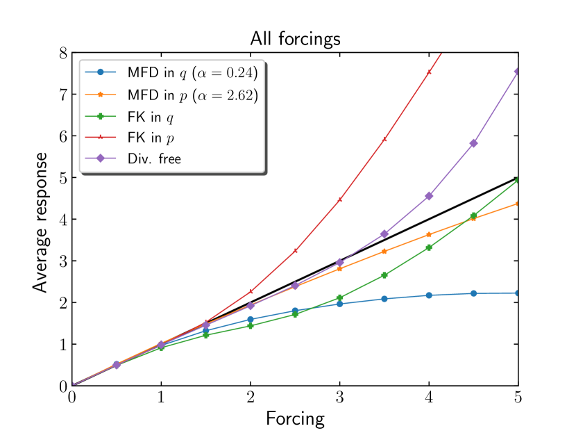
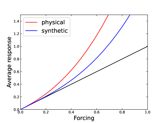
where F𝐹F is the external forcing and η𝜂\eta\in\mathbb{R} its magnitude, and Wtsubscript𝑊𝑡W_{t} a standard Brownian motion. In general, it is observed that the response 𝔼η(R)subscript𝔼𝜂𝑅\mathbb{E}_{\eta}(R) of the system, given by the steady-state average of a physical observable R𝑅R of interest which has average 0 for unperturbed dynamics (η=0𝜂0\eta=0), is proportional to the magnitude of the forcing for small values of the forcing. This corresponds to the linear response regime; see Figure 1. When this is the case, the linear response ρ1subscript𝜌1\rho_{1} is computed as

(2) ρ1=limη0𝔼η(R)η.subscript𝜌1subscript𝜂0subscript𝔼𝜂𝑅𝜂\rho_{1}=\lim_{\eta\to 0}\frac{\mathbb{E}_{\eta}(R)}{\eta}.

By definition, transport coefficients are the proportionality constants ρ1subscript𝜌1\rho_{1} relating the response 𝔼η(R)subscript𝔼𝜂𝑅\mathbb{E}_{\eta}(R) to the forcing for |η|𝜂|\eta| small. One typical example is the case where the force F𝐹F is constant and the configuration space is a torus. Such a forcing is considered to compute the mobility of particles in the system, which we discuss in more detail in Section 2.2.3. Another example is the case where F𝐹F has components in one direction only, whose magnitude depends on the position in another direction. Such forcings can be used to estimate the shear viscosity through the so-called sinusoidal transverse force method [19].

In practice, steady-state averages involved in the linear response are computed as ergodic averages over a very long trajectory of the system, obtained as a realization of the stochastic differential equation (SDE) (9). Although there are several such ways of computing these steady-state averages, it is typically done in one of two ways: either based on (i) equilibrium techniques based on Green–Kubo formulae, which are integrated autocorrelation functions [20, 26]; or (ii) nonequilibrium steady-state methods where the limit (2) is numerically estimated; see [6]. Both numerical methods have advantages and drawbacks, and are constantly undergoing algorithmic advances; see [7, 37], and [43] for a comparison and discussion between the methods. In this work, however, we focus exclusively on the nonequilibrium approach.

In the NEMD approach, a standard estimator to compute the linear response (2) is

(3) Φ^η,t=1ηt0tR(Xsη)𝑑s,subscript^Φ𝜂𝑡1𝜂𝑡superscriptsubscript0𝑡𝑅superscriptsubscript𝑋𝑠𝜂differential-d𝑠\widehat{\Phi}_{\eta,t}=\frac{1}{\eta t}\int_{0}^{t}R(X_{s}^{\eta})\,ds,

where the fixed value of η0𝜂0\eta\neq 0 should be small enough in absolute value in order for the nonlinear part of the response to be negligible. Although there are various sources of error associated with the estimator (3), as made precise in Section 2.3, the variance associated with (3) is the main issue. In particular, in the context of computing transport coefficients, the large signal-to-noise ratio leads to a very large statistical error, as we are averaging very small linear responses [42]. The estimator (3), for instance, has asymptotic variance of order O(t1η2)Osuperscript𝑡1superscript𝜂2\mathrm{O}(t^{-1}\eta^{-2}), much larger than the usual asymptotic variance of order O(t1)Osuperscript𝑡1\mathrm{O}(t^{-1}) associated with its equilibrium averages counterpart, as the linear regime is only valid for |η|1much-less-than𝜂1|\eta|\ll 1. This motivates the interest of variance reduction techniques, which are used to decrease the statistical error in the estimated averages. Examples of standard variance reduction techniques for Monte Carlo simulations, for which a review is provided in [5], are antithetic variables, stratification, control variate methods and importance sampling.

One of the main challenges with computing nonequilibrium steady-state averages, however, is that traditional equilibrium variance reduction techniques cannot be used the same way (see [29, Section 5.4] for a detailed discussion on obstructions to this end). Although many practitioners of molecular dynamics realize that the computation of transport coefficients is a difficult numerical issue, there were only a handful of attempts to develop dedicated variance reduction techniques. Many practitioners still use direct, brute force numerical methods based on a time integration of the dynamics.

In order to reduce the statistical error of order 1/(η2t)1superscript𝜂2𝑡1/(\eta^{2}t), one idea is to extend the regime of linear response, which consequently allows to use larger values of η𝜂\eta. One approach for doing so is to use synthetic forcings. Such forcings, as presented in this work, were introduced by Evans and Morriss [11] (“synthetic fields”, in their terminology) with the purpose to produce a mechanical analog of a thermal transport process. This notion was originally used by Gillan and Dixon [18], then abstracted and extended by Evans and Morriss in [11]. The name synthetic is used to denote that the external fields under consideration do not exist in nature.

The key idea behind synthetic forcings is that there are infinitely many forcings which lead to the same transport coefficient. This flexibility should be used to develop better numerical methods for the computation of transport coefficients. In theory, one can add an extra forcing to the physical perturbation of the system, as long as this extra forcing preserves the invariant measure of the reference system, which in turn preserves the linear response. We call the resulting perturbation a synthetic forcing, as it has no physical representation; it is a mathematical device used to simplify the problem at hand.

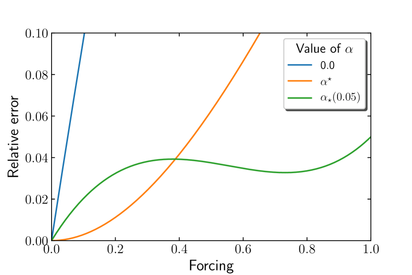
The aim is to find synthetic perturbations allowing to reduce the nonlinear part of the response as much as possible (see Figure 1) in order to consider larger values of |η|𝜂|\eta|. In this article, we present a mathematical framework for choosing and quantifying the quality of synthetic forcings, in the context of linear response theory, and discuss various possible choices for them. We illustrate the analysis with numerical results in low dimensional systems.
Refer to caption
Figure 1: Illustration of the effect of synthetic forcings. Ideally, the nonlinear part of the average response 𝔼η(R)subscript𝔼𝜂𝑅\mathbb{E}_{\eta}(R) is smaller, so that 𝔼η(R)ρ1ηsubscript𝔼𝜂𝑅subscript𝜌1𝜂\mathbb{E}_{\eta}(R)\approx\rho_{1}\eta for larger values of |η|𝜂|\eta| than with physical forcings.

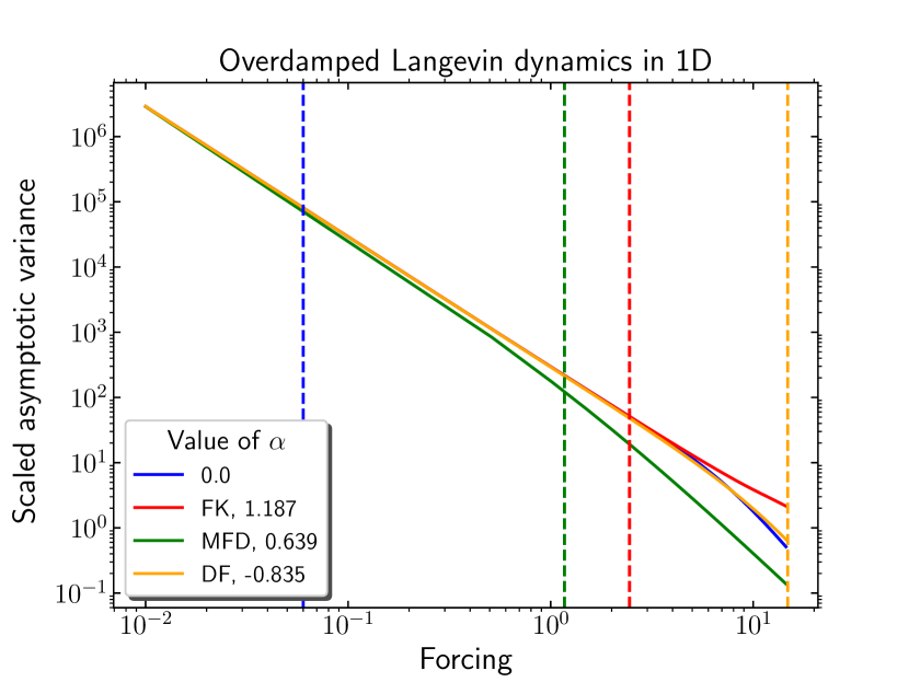
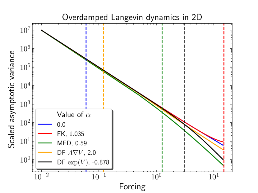
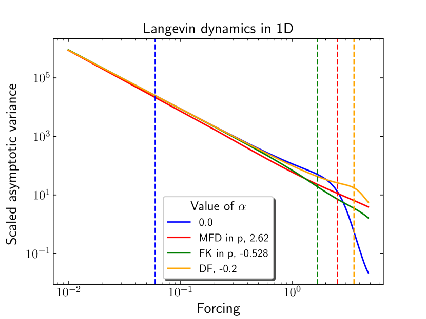
This work is organized as follows. We present in Section 2 a review of linear response theory and associated computational techniques, and state technical results which make precise some error estimates, in particular bounds on the asymptotic variance of time averages such as (3). We then introduce the notion of synthetic forcings in Section 3, where we also give examples and discuss them in more detail. We next demonstrate the possibly dramatic benefits in terms of statistical error with some numerical results in low dimensions in Section 4, namely one and two-dimensional overdamped Langevin dynamics, and one-dimensional Langevin dynamics. We finally discuss in Section 5 the extensions and perspectives of this approach.

2 Linear response and associated computational techniques

In this section, we review linear response theory and the computational techniques allowing to compute transport coefficients. The framework we consider is that of stochastic dynamics, ergodic for the Boltzmann–Gibbs measure, which are perturbed by external forcings.

We start in Section 2.1 by setting up the framework for general time-homogeneous SDEs, and the specific dynamics we consider, namely (non)equilibrium overdamped Langevin and Langevin dynamics. We then review in Section 2.2 linear response theory, the definition of transport coefficients and discuss the associated standard numerical techniques to estimate these coefficients. We finally present the numerical analysis of nonequilibrium molecular dynamics in Section 2.3.

2.1 Reference dynamics and perturbation

We start by describing in Section 2.1.1 the general setting for linear response theory for a general stochastic differential equation (SDE). We introduce in particular some assumptions on the dynamics which will be used in the analysis throughout this paper. We next describe the dynamics and their nonequilibrium perturbations for overdamped Langevin and Langevin dynamics in Sections 2.1.2 and 2.1.3, respectively.

2.1.1 General setting

Reference dynamics

Consider a general time-homogeneous SDE defined on the state-space 𝒳𝒳\mathcal{X}, where 𝒳𝒳\mathcal{X} is typically the full space dsuperscript𝑑\mathbb{R}^{d} or a bounded domain with periodic boundary conditions 𝕋dsuperscript𝕋𝑑\mathbb{T}^{d} (with 𝕋=/𝕋\mathbb{T}=\mathbb{R}/\mathbb{Z} the one-dimensional torus):

(4) dXt=b(Xt)dt+σ(Xt)dWt,𝑑subscript𝑋𝑡𝑏subscript𝑋𝑡𝑑𝑡𝜎subscript𝑋𝑡𝑑subscript𝑊𝑡dX_{t}=b(X_{t})\,dt+\sigma(X_{t})\,dW_{t},

for a given initial condition x0𝒳subscript𝑥0𝒳x_{0}\in\mathcal{X}, a standard Brownian motion Wtmsubscript𝑊𝑡superscript𝑚W_{t}\in\mathbb{R}^{m}, and where b:𝒳d:𝑏𝒳superscript𝑑b\colon\mathcal{X}\to\mathbb{R}^{d} and σ:𝒳d×m:𝜎𝒳superscript𝑑𝑚\sigma\colon\mathcal{X}\to\mathbb{R}^{d\times m} are assumed to be such that there exists a unique solution to (4). A simple setting is to assume that b𝑏b and σ𝜎\sigma are Csuperscript𝐶C^{\infty}, hence locally Lipschitz, which is used to prove existence and uniqueness of the solution [40, 33, 22]. The SDE (4) is associated with the following infinitesimal generator

(5) 0=bT+12σσT:2,:subscript0superscript𝑏𝑇12𝜎superscript𝜎𝑇superscript2\mathcal{L}_{0}=b^{T}\nabla+\frac{1}{2}\sigma\sigma^{T}\colon\nabla^{2},

where ::: denotes the Frobenius inner product, and 2superscript2\nabla^{2} is the Hessian operator. More explicitly, for some given Csuperscript𝐶C^{\infty} test function φ:d:𝜑superscript𝑑\varphi\colon\mathbb{R}^{d}\to\mathbb{R}, the operator 0subscript0\mathcal{L}_{0} acts as

(6) 0φ=i=1dbixiφ+12i=1dj=1dk=1mσi,kσj,kxi,xj2φ.subscript0𝜑superscriptsubscript𝑖1𝑑subscript𝑏𝑖subscriptsubscript𝑥𝑖𝜑12superscriptsubscript𝑖1𝑑superscriptsubscript𝑗1𝑑superscriptsubscript𝑘1𝑚subscript𝜎𝑖𝑘subscript𝜎𝑗𝑘subscriptsuperscript2subscript𝑥𝑖subscript𝑥𝑗𝜑\mathcal{L}_{0}\varphi=\sum_{i=1}^{d}b_{i}\partial_{x_{i}}\varphi+\frac{1}{2}\sum_{i=1}^{d}\sum_{j=1}^{d}\sum_{k=1}^{m}\sigma_{i,k}\sigma_{j,k}\partial^{2}_{x_{i},x_{j}}\varphi.

We assume that the dynamics (4) has a unique invariant probability measure with a density with respect to the Lebesgue measure denoted by ψ0(x)subscript𝜓0𝑥\psi_{0}(x). This density satisfies the stationary Fokker–Planck equation

(7) 0ψ0=0,superscriptsubscript0subscript𝜓00\mathcal{L}_{0}^{\dagger}\psi_{0}=0,

where 0superscriptsubscript0\mathcal{L}_{0}^{\dagger} denotes the L2superscript𝐿2L^{2}-adjoint of the operator 0subscript0\mathcal{L}_{0}, acting as

(8) 0φ=div(bφ)+122:(σσTφ).:superscriptsubscript0𝜑div𝑏𝜑12superscript2𝜎superscript𝜎𝑇𝜑\mathcal{L}_{0}^{\dagger}\varphi=-\operatorname{div}(b\varphi)+\frac{1}{2}\nabla^{2}:\left(\sigma\sigma^{T}\varphi\right).
Perturbation of the reference dynamics

We next consider a perturbation of the reference dynamics (4), obtained by adding to the drift field b𝑏b some smooth nongradient forcing F:𝒳d:𝐹𝒳superscript𝑑F\colon\mathcal{X}\to\mathbb{R}^{d} of magnitude η𝜂\eta\in\mathbb{R}:

(9) dXtη=(b(Xtη)+ηF(Xtη))dt+σ(Xtη)dWt.𝑑superscriptsubscript𝑋𝑡𝜂𝑏superscriptsubscript𝑋𝑡𝜂𝜂𝐹superscriptsubscript𝑋𝑡𝜂𝑑𝑡𝜎superscriptsubscript𝑋𝑡𝜂𝑑subscript𝑊𝑡dX_{t}^{\eta}=\left(b(X_{t}^{\eta})+\eta F(X_{t}^{\eta})\right)dt+\sigma(X_{t}^{\eta})\,dW_{t}.

The generator of (9) is denoted by η=0+η~physsubscript𝜂subscript0𝜂subscript~phys\mathcal{L}_{\eta}=\mathcal{L}_{0}+\eta\widetilde{\mathcal{L}}_{\mathrm{phys}}, where ~physsubscript~phys\widetilde{\mathcal{L}}_{\mathrm{phys}} is the generator associated with the physical perturbation:

(10) ~phys=FT.subscript~physsuperscript𝐹𝑇\widetilde{\mathcal{L}}_{\mathrm{phys}}=F^{T}\nabla.

We assume that b𝑏b, σ𝜎\sigma and F𝐹F are such that the following assumption holds.

Assumption 1 (Uniqueness of the invariant measure).

The dynamics (9) admits a unique invariant probability measure for any η𝜂\eta\in\mathbb{R}, with a smooth density ψηsubscript𝜓𝜂\psi_{\eta} with respect to the Lebesgue measure. Moreover, trajectorial ergodicity holds: for any observable R𝑅absentR\in L1(ψη)superscript𝐿1subscript𝜓𝜂L^{1}\left(\psi_{\eta}\right), and any initial condition X0ηsuperscriptsubscript𝑋0𝜂X_{0}^{\eta},

(11) 𝔼η(R):=R(x)ψη(x)𝑑x=limT1T0TR(Xtη)𝑑t a.s. formulae-sequenceassignsubscript𝔼𝜂𝑅subscript𝑅𝑥subscript𝜓𝜂𝑥differential-d𝑥subscript𝑇1𝑇superscriptsubscript0𝑇𝑅superscriptsubscript𝑋𝑡𝜂differential-d𝑡 a.s. \mathbb{E}_{\eta}(R):=\int_{\mathcal{M}}R(x)\psi_{\eta}(x)\,dx=\lim_{T\rightarrow\infty}\frac{1}{T}\int_{0}^{T}R(X_{t}^{\eta})\,dt\quad\text{ a.s. }

Note that ψηsubscript𝜓𝜂\psi_{\eta} solves the Fokker–Planck equation

(12) (0+η~phys)ψη=0.superscriptsubscript0𝜂subscript~physsubscript𝜓𝜂0\left(\mathcal{L}_{0}+\eta\widetilde{\mathcal{L}}_{\mathrm{phys}}\right)^{\dagger}\psi_{\eta}=0.

Sufficient conditions for Assumption 1 to hold are discussed after Assumption 2 below. Although ψηsubscript𝜓𝜂\psi_{\eta} can be shown to uniquely exist, its analytical expression is generally not known. Note that in the case η=0𝜂0\eta=0, the dynamics (9) reduces to the reference dynamics (4).

We need to make precise some estimates on the evolution semigroup associated with (9) for the analysis presented in Section 2.3. We consider to this end weighted spaces of bounded functions. To define them, we first introduce a family of Lyapunov functions denoted by (𝒦n)nsubscriptsubscript𝒦𝑛𝑛(\mathcal{K}_{n})_{n\in\mathbb{N}}, with 𝒦n:𝒳[1,+):subscript𝒦𝑛𝒳1\mathcal{K}_{n}\colon\mathcal{X}\to[1,+\infty) such that

(13) n0,𝒦n𝒦n+1.formulae-sequencefor-all𝑛0subscript𝒦𝑛subscript𝒦𝑛1\forall n\geqslant 0,\qquad\mathcal{K}_{n}\leqslant\mathcal{K}_{n+1}.

The associated weighted Bsuperscript𝐵B^{\infty} spaces are

(14) Bn={φ measurable|φBn:=supx𝒳|φ(x)𝒦n(x)|<+}.superscriptsubscript𝐵𝑛conditional-set𝜑 measurableassignsubscriptnorm𝜑superscriptsubscript𝐵𝑛subscriptsupremum𝑥𝒳𝜑𝑥subscript𝒦𝑛𝑥B_{n}^{\infty}=\left\{\varphi\text{ measurable}\,\middle|\,\|\varphi\|_{B_{n}^{\infty}}:=\sup_{x\in\mathcal{X}}\left|\frac{\varphi(x)}{\mathcal{K}_{n}(x)}\right|<+\infty\right\}.

In particular, for any φBm𝜑subscriptsuperscript𝐵𝑚\varphi\in B^{\infty}_{m}, it holds that |φ|φBm𝒦m𝜑subscriptnorm𝜑subscriptsuperscript𝐵𝑚subscript𝒦𝑚|\varphi|\leqslant\|\varphi\|_{B^{\infty}_{m}}\mathcal{K}_{m}. We can then introduce the space 𝒮𝒮\mathscr{S}, which consists of all functions φC(𝒳)𝜑superscript𝐶𝒳\varphi\in C^{\infty}(\mathcal{X}) which grow at most like 𝒦nsubscript𝒦𝑛\mathcal{K}_{n} for some n𝑛n, and whose derivates also grow at most like 𝒦msubscript𝒦𝑚\mathcal{K}_{m}, possibly with m>n𝑚𝑛m>n and m𝑚m depending on the order of derivation. Denoting by k=x1k1xdkdsuperscript𝑘superscriptsubscriptsubscript𝑥1subscript𝑘1superscriptsubscriptsubscript𝑥𝑑subscript𝑘𝑑\partial^{k}=\partial_{x_{1}}^{k_{1}}\dotsc\partial_{x_{d}}^{k_{d}} for k=(k1,,kd)d𝑘subscript𝑘1subscript𝑘𝑑superscript𝑑k=(k_{1},\dotsc,k_{d})\in\mathbb{N}^{d},

(15) 𝒮={φC(𝒳)|kd,n,kφBn}.𝒮conditional-set𝜑superscript𝐶𝒳formulae-sequencefor-all𝑘superscript𝑑formulae-sequence𝑛superscript𝑘𝜑superscriptsubscript𝐵𝑛\mathscr{S}=\left\{\varphi\in C^{\infty}\left(\mathcal{X}\right)\,\middle|\,\forall k\in\mathbb{N}^{d},\;\exists n\in\mathbb{N},\;\partial^{k}\varphi\in B_{n}^{\infty}\right\}.

When 𝒳𝒳\mathcal{X} is bounded, it is possible to choose 𝒦n=1subscript𝒦𝑛1\mathcal{K}_{n}=1 for all n0𝑛0n\geqslant 0, in which case 𝒮=C(𝒳)𝒮superscript𝐶𝒳\mathscr{S}=C^{\infty}(\mathcal{X}). For unbounded spaces, a typical choice is 𝒦n=1+|x|nsubscript𝒦𝑛1superscript𝑥𝑛\mathcal{K}_{n}=1+|x|^{n}, in which case the functions φ𝒮𝜑𝒮\varphi\in\mathscr{S} and their derivatives grow at most polynomially. We also consider the subspace 𝒮0=Π0𝒮subscript𝒮0subscriptΠ0𝒮\mathscr{S}_{0}=\Pi_{0}\mathscr{S} of functions with average 0 with respect to ψ0subscript𝜓0\psi_{0}, where ΠηsubscriptΠ𝜂\Pi_{\eta} for η𝜂\eta\in\mathbb{R} denotes the projection operator

(16) Πηφ=φ𝒳φψη.subscriptΠ𝜂𝜑𝜑subscript𝒳𝜑subscript𝜓𝜂\Pi_{\eta}\varphi=\varphi-\int_{\mathcal{X}}\varphi\,\psi_{\eta}.

We denote by (E)\|\cdot\|_{\mathcal{B}(E)} the operator norm on the Banach space (E)𝐸\mathcal{B}(E) of bounded linear operators on a Banach space E𝐸E, defined by

(17) 𝒜(E)=supgE{0}𝒜gEgE.subscriptnorm𝒜𝐸subscriptsupremum𝑔𝐸0subscriptnorm𝒜𝑔𝐸subscriptnorm𝑔𝐸\|\mathcal{A}\|_{\mathcal{B}(E)}=\sup_{g\in E\setminus\{0\}}\frac{\|\mathcal{A}g\|_{E}}{\|g\|_{E}}.

Before we state the next assumption, we let 𝒜superscript𝒜\mathcal{A}^{*} denote the adjoint of 𝒜𝒜\mathcal{A} on the space L2(ψ0)superscript𝐿2subscript𝜓0L^{2}(\psi_{0}). More explicitly, for any test functions φ,ϕC𝜑italic-ϕsuperscript𝐶\varphi,\phi\in C^{\infty} with compact support,

(18) 𝒳(𝒜φ)ϕψ0=𝒳φ(𝒜ϕ)ψ0.subscript𝒳𝒜𝜑italic-ϕsubscript𝜓0subscript𝒳𝜑superscript𝒜italic-ϕsubscript𝜓0\int_{\mathcal{X}}(\mathcal{A}\varphi)\phi\,\psi_{0}=\int_{\mathcal{X}}\varphi(\mathcal{A}^{*}\phi)\,\psi_{0}.

The action of these operators can be found via integration by parts. In particular, for ψ0(x)subscript𝜓0𝑥\psi_{0}(x) a probability density proportional to eβU(x)superscripte𝛽𝑈𝑥\mathrm{e}^{-\beta U(x)}, an integration by parts shows that xi=xi+βxiUsuperscriptsubscriptsubscript𝑥𝑖subscriptsubscript𝑥𝑖𝛽subscriptsubscript𝑥𝑖𝑈\partial_{x_{i}}^{*}=-\partial_{x_{i}}+\beta\partial_{x_{i}}U. In addition, note that xx=i=1dxixisuperscriptsubscript𝑥subscript𝑥superscriptsubscript𝑖1𝑑superscriptsubscriptsubscript𝑥𝑖subscriptsubscript𝑥𝑖\nabla_{x}^{*}\nabla_{x}=\sum_{i=1}^{d}\partial_{x_{i}}^{*}\partial_{x_{i}}.

Note that the Fokker–Planck equation (7), written in terms of the L2superscript𝐿2L^{2}-adjoint, can also be written with the L2(ψ0)superscript𝐿2subscript𝜓0L^{2}(\psi_{0})-adjoint as 0𝟏=0superscriptsubscript010\mathcal{L}_{0}^{*}\mathbf{1}=0. We make the following assumption on the Lyapunov functions.

Assumption 2 (Lyapunov estimates).

The space 𝒮𝒮\mathscr{S} is dense in L2(ψη)superscript𝐿2subscript𝜓𝜂L^{2}(\psi_{\eta}) for any η𝜂\eta\in\mathbb{R}. For any n𝑛n\in\mathbb{N}, the L2(ψη)superscript𝐿2subscript𝜓𝜂L^{2}(\psi_{\eta}) norms of the Lyapunov functions are uniformly bounded on compact sets of η𝜂\eta: for any η>0subscript𝜂0\eta_{*}>0, there exists a constant Cn,η<+subscript𝐶𝑛subscript𝜂C_{n,\eta_{*}}<+\infty such that

(19) |η|η,𝒦nL2(ψη)Cn,η.formulae-sequencefor-all𝜂subscript𝜂subscriptnormsubscript𝒦𝑛superscript𝐿2subscript𝜓𝜂subscript𝐶𝑛subscript𝜂\forall|\eta|\leqslant\eta_{*},\quad\left\|\mathcal{K}_{n}\right\|_{L^{2}\left(\psi_{\eta}\right)}\leqslant C_{n,\eta_{*}}.

Moreover ηsubscript𝜂-\mathcal{L}_{\eta} is invertible on ΠηBnsubscriptΠ𝜂superscriptsubscript𝐵𝑛\Pi_{\eta}B_{n}^{\infty}, and the inverse generator is bounded uniformly on compact sets of η𝜂\eta:

(20) |η|η,η1(ΠηBn)Kn,η.formulae-sequencefor-all𝜂subscript𝜂subscriptnormsuperscriptsubscript𝜂1subscriptΠ𝜂superscriptsubscript𝐵𝑛subscript𝐾𝑛subscript𝜂\forall|\eta|\leqslant\eta_{*},\quad\left\|-\mathcal{L}_{\eta}^{-1}\right\|_{\mathcal{B}\left(\Pi_{\eta}B_{n}^{\infty}\right)}\leqslant K_{n,\eta_{*}}.

Additionally,

(21) |η|η,n1,supt+etη𝒦nBnMn,η<+formulae-sequencefor-all𝜂subscript𝜂formulae-sequencefor-all𝑛1subscriptsupremum𝑡subscriptsubscriptnormsuperscripte𝑡subscript𝜂subscript𝒦𝑛subscriptsuperscript𝐵𝑛subscript𝑀𝑛subscript𝜂\forall|\eta|\leqslant\eta_{*},\quad\forall n\geqslant 1,\qquad\sup_{t\in\mathbb{R}_{+}}\left\|\mathrm{e}^{t\mathcal{L}_{\eta}}\mathcal{K}_{n}\right\|_{B^{\infty}_{n}}\leqslant M_{n,\eta_{*}}<+\infty

We finally assume that for any n,n𝑛superscript𝑛n,n^{\prime}\in\mathbb{N}, there exists m𝑚m\in\mathbb{N} such that 𝒦n𝒦nBmsubscript𝒦𝑛subscript𝒦superscript𝑛subscriptsuperscript𝐵𝑚\mathcal{K}_{n}\mathcal{K}_{n^{\prime}}\in B^{\infty}_{m}.

The estimates (19) through (21) are usually obtained from Lyapunov conditions of the form

(22) η𝒦nan,η𝒦n+bn,η,subscript𝜂subscript𝒦𝑛subscript𝑎𝑛𝜂subscript𝒦𝑛subscript𝑏𝑛𝜂\mathcal{L}_{\eta}\mathcal{K}_{n}\leqslant-a_{n,\eta}\mathcal{K}_{n}+b_{n,\eta},

for some an,η>0subscript𝑎𝑛𝜂0a_{n,\eta}>0 and bn,ηsubscript𝑏𝑛𝜂b_{n,\eta}\in\mathbb{R}. After integration against ψηsubscript𝜓𝜂\psi_{\eta}, and making use of the invariance of ψηsubscript𝜓𝜂\psi_{\eta} by the dynamics,

(23) 0=𝒳η𝒦nψηan,η𝒳𝒦nψη+bn,η,0subscript𝒳subscript𝜂subscript𝒦𝑛subscript𝜓𝜂subscript𝑎𝑛𝜂subscript𝒳subscript𝒦𝑛subscript𝜓𝜂subscript𝑏𝑛𝜂0=\int_{\mathcal{X}}\mathcal{L}_{\eta}\mathcal{K}_{n}\,\psi_{\eta}\leqslant-a_{n,\eta}\int_{\mathcal{X}}\mathcal{K}_{n}\,\psi_{\eta}+b_{n,\eta},

so that

(24) 1𝒳𝒦nψηbn,ηan,η.1subscript𝒳subscript𝒦𝑛subscript𝜓𝜂subscript𝑏𝑛𝜂subscript𝑎𝑛𝜂1\leqslant\int_{\mathcal{X}}\mathcal{K}_{n}\,\psi_{\eta}\leqslant\frac{b_{n,\eta}}{a_{n,\eta}}.

The condition (19) then follows from the last statement of Assumption 2 since, for any n1𝑛1n\geqslant 1, there exists Cn>0subscript𝐶𝑛0C_{n}>0 and m1𝑚1m\geqslant 1 such that 1𝒦n2Cn𝒦m1superscriptsubscript𝒦𝑛2subscript𝐶𝑛subscript𝒦𝑚1\leqslant\mathcal{K}_{n}^{2}\leqslant C_{n}\mathcal{K}_{m}. Condition (22) also implies the existence of an invariant probability measure for any η𝜂\eta\in\mathbb{R} when a minorization condition holds [21]. The minorization condition typically follows from a controllability argument and (hypo)ellipticity conditions, see for instance [34, 40]. As for Assumption 1, trajectorial ergodicity holds when the generator ηsubscript𝜂\mathcal{L}_{\eta} is either elliptic or hypoelliptic, and there exists an invariant probability measure with positive density with respect to the Lebesgue measure [23].

We need an assumption in our analysis on the generator 0subscript0\mathcal{L}_{0} of the reference dynamics, which will be useful when stating some technical results later on.

Assumption 3 (Stability of smooth functions by inverse operators).

The space 𝒮𝒮\mathscr{S} is stable by the generator 0subscript0\mathcal{L}_{0}, and 0subscript0\mathcal{L}_{0} and 0superscriptsubscript0\mathcal{L}_{0}^{*} are invertible on 𝒮0subscript𝒮0\mathscr{S}_{0}. This means that, for any φ𝒮0𝜑subscript𝒮0\varphi\in\mathscr{S}_{0}, there exists a unique solution Ψ𝒮0Ψsubscript𝒮0\Psi\in\mathscr{S}_{0} to the Poisson equation 0Ψ=φsubscript0Ψ𝜑-\mathcal{L}_{0}\Psi=\varphi.

The generator of the perturbation should also satisfy the next assumption.

Assumption 4 (Stability of smooth functions by the perturbation operator).

The generator ~physsubscript~phys\widetilde{\mathcal{L}}_{\mathrm{phys}} of the perturbation is such that 𝒮𝒮\mathscr{S} is stable by ~physsubscript~phys\widetilde{\mathcal{L}}_{\mathrm{phys}}, and ~phys𝒮𝒮0superscriptsubscript~phys𝒮subscript𝒮0\widetilde{\mathcal{L}}_{\mathrm{phys}}^{*}\mathscr{S}\subset~{}\mathscr{S}_{0}.

Assumption 4 is easily seen to be satisfied for perturbations ~physsubscript~phys\widetilde{\mathcal{L}}_{\mathrm{phys}} of the form FTsuperscript𝐹𝑇F^{T}\nabla when F𝐹F has components in 𝒮𝒮\mathscr{S}, which is assumed here and for the remainder of this work. A simple computation based on integrations by parts shows that ~phys𝒮𝒮0superscriptsubscript~phys𝒮subscript𝒮0\widetilde{\mathcal{L}}_{\mathrm{phys}}^{*}\mathscr{S}\subset\mathscr{S}_{0} when ~phys𝟏=0subscript~phys10\widetilde{\mathcal{L}}_{\mathrm{phys}}\mathbf{1}=0. Indeed, for φ𝒮𝜑𝒮\varphi\in\mathscr{S}, using the definition of the L2(ψ0)superscript𝐿2subscript𝜓0L^{2}(\psi_{0})-adjoint,

(25) 𝒳~physφψ0=𝒳φ(~phys𝟏)ψ0=0.subscript𝒳superscriptsubscript~phys𝜑subscript𝜓0subscript𝒳𝜑subscript~phys1subscript𝜓00\int_{\mathcal{X}}\widetilde{\mathcal{L}}_{\mathrm{phys}}^{*}\varphi\,\psi_{0}=\int_{\mathcal{X}}\varphi\left(\widetilde{\mathcal{L}}_{\mathrm{phys}}\mathbf{1}\right)\,\psi_{0}=0.

One function of particular interest in the range of ~physsuperscriptsubscript~phys\widetilde{\mathcal{L}}_{\mathrm{phys}}^{*} is the conjugate response function

(26) S=~phys𝟏,𝑆superscriptsubscript~phys1S=\widetilde{\mathcal{L}}_{\mathrm{phys}}^{*}\mathbf{1},

which we introduce here as it will be useful later. Note that the expression for S𝑆S comes from the generator ~physsubscript~phys\widetilde{\mathcal{L}}_{\mathrm{phys}} of the perturbation, and not the observable R𝑅R. Let us emphasize that beyond the case of physical forcings FTsuperscript𝐹𝑇F^{T}\nabla, Assumption 4 will be needed for more general operators in Section 3.

Assumptions 1 through 4 are natural for overdamped Langevin and Langevin dynamics, which we present in the next two sections.

2.1.2 Overdamped Langevin dynamics

One typical dynamics used in molecular dynamics is overdamped Langevin dynamics, which evolves only the positions q𝑞q of the system.

Reference dynamics

Mathematically, the overdamped Langevin dynamics corresponds to the following SDE with nondegenerate noise:

(27) dqt=V(qt)dt+2βdWt,𝑑subscript𝑞𝑡𝑉subscript𝑞𝑡𝑑𝑡2𝛽𝑑subscript𝑊𝑡dq_{t}=-\nabla V(q_{t})\,dt+\sqrt{\frac{2}{\beta}}\,dW_{t},

where β>0𝛽0\beta>0 is proportional to the inverse temperature, and V𝑉V is a smooth potential. The generator associated with (27) is given by

(28) 0=VT+1βΔ,subscript0superscript𝑉𝑇1𝛽Δ\mathcal{L}_{0}=-\nabla V^{T}\nabla+\frac{1}{\beta}\Delta,

with L2(𝒳)superscript𝐿2𝒳L^{2}(\mathcal{X})-adjoint

(29) 0superscriptsubscript0\displaystyle\mathcal{L}_{0}^{\dagger} =div(V)+1βΔ.\displaystyle=\operatorname{div}(\nabla V\cdot)+\frac{1}{\beta}\Delta.

The dynamics (27) admits the Gibbs measure with density

(30) ψ0(q)=1ZeβV(q),Z=𝒳eβV(q)𝑑q<+formulae-sequencesubscript𝜓0𝑞1𝑍superscripte𝛽𝑉𝑞𝑍subscript𝒳superscripte𝛽𝑉𝑞differential-d𝑞\psi_{0}(q)=\frac{1}{Z}\mathrm{e}^{-\beta V(q)},\qquad Z=\int_{\mathcal{X}}\mathrm{e}^{-\beta V(q)}dq<+\infty

as its unique invariant probability measure. It can indeed be checked that 0ψ0=0superscriptsubscript0subscript𝜓00\mathcal{L}_{0}^{\dagger}\psi_{0}=0, so that ψ0subscript𝜓0\psi_{0} is a stationary solution to the Fokker–Planck equation. Here and in the remainder of this work, we assume that eβVL1(𝒳)superscripte𝛽𝑉superscript𝐿1𝒳\mathrm{e}^{-\beta V}\in L^{1}(\mathcal{X}). Note that the generator (28) is self-adjoint on the Hilbert space L2(ψ0)superscript𝐿2subscript𝜓0L^{2}(\psi_{0}), as 0=β1subscript0superscript𝛽1superscript\mathcal{L}_{0}=-\beta^{-1}\nabla^{*}\nabla.

Nonequilibrium perturbation

The perturbed overdamped Langevin dynamics corresponding to (9) reads

(31) dqtη=(V(qtη)+ηF(qtη))dt+2βdWt.𝑑superscriptsubscript𝑞𝑡𝜂𝑉superscriptsubscript𝑞𝑡𝜂𝜂𝐹superscriptsubscript𝑞𝑡𝜂𝑑𝑡2𝛽𝑑subscript𝑊𝑡dq_{t}^{\eta}=\left(-\nabla V(q_{t}^{\eta})+\eta F(q_{t}^{\eta})\right)dt+\sqrt{\frac{2}{\beta}}\,dW_{t}.

It has generator η=0+η~physsubscript𝜂subscript0𝜂subscript~phys\mathcal{L}_{\eta}=\mathcal{L}_{0}+\eta\widetilde{\mathcal{L}}_{\mathrm{phys}}, where ~phys=FTsubscript~physsuperscript𝐹𝑇\widetilde{\mathcal{L}}_{\mathrm{phys}}=F^{T}\nabla. Recall that F𝐹F is assumed to be nongradient, so that in general there is no explicit expression for the invariant probability measure of (31) when such a measure exists.

Remark 2.1.

One of the only cases where a closed form for ψηsubscript𝜓𝜂\psi_{\eta} is known is the one-dimensional case for overdamped Langevin dynamics, where the associated Fokker–Planck equation is directly solvable, as discussed for instance in [13], which generalizes the computations of [39, Section 2.5].

Conditions for assumptions to be satisfied

We now discuss the conditions under which Assumptions 1 through 4 are satisfied for the perturbed overdamped Langevin dynamics (31), which correspond to standard results in the literature.

  • If the space 𝒳𝒳\mathcal{X} is compact, then it is trivial to satisfy the Lyapunov condition (22) by choosing 𝒦n=𝟏subscript𝒦𝑛1\mathcal{K}_{n}=\mathbf{1}. In the case of unbounded spaces, a typical choice is 𝒦n=1+|q|nsubscript𝒦𝑛1superscript𝑞𝑛\mathcal{K}_{n}=1+|q|^{n}, with the condition that there exist A>0𝐴0A>0 and B𝐵B\in\mathbb{R} such that

    (32) qTV(q)A|q|2B.superscript𝑞𝑇𝑉𝑞𝐴superscript𝑞2𝐵q^{T}\nabla V(q)\geqslant A|q|^{2}-B.

    Condition (32) is satisfied for potentials V(q)𝑉𝑞V(q) that behave as |q|ksuperscript𝑞𝑘|q|^{k} for k2𝑘2k\geqslant 2 at infinity. This ensures that the dynamics returns to some compact region around the origin.

  • Assumption 1 can be shown to hold using Lyapunov techniques and a minorization condition [34, 40, 24]. It can thus be shown that the dynamics (31) has a unique invariant probability measure with positive density with respect to the Lebesgue measure, and therefore that trajectorial ergodicity holds.

  • Assumptions 2 and 3 hold under some conditions on the potential V𝑉V, which include (32); see [24] for a precise discussion.

  • Lastly, Assumption 4 is trivially satisfied, as ~phys=FTqsubscript~physsuperscript𝐹𝑇subscript𝑞\widetilde{\mathcal{L}}_{\mathrm{phys}}=F^{T}\nabla_{q} leaves 𝒮𝒮\mathscr{S} stable when F𝒮𝐹𝒮F\in\mathscr{S}, and ~phys𝒮𝒮0superscriptsubscript~phys𝒮subscript𝒮0\widetilde{\mathcal{L}}_{\mathrm{phys}}^{*}\mathscr{S}\subset\mathscr{S}_{0} in view of (25).

2.1.3 Langevin dynamics

Another dynamics of interest used in molecular dynamics is Langevin dynamics, which can be seen as a Hamiltonian dynamics perturbed by an Ornstein–Uhlenbeck process on the momenta. Mathematically, it corresponds to an SDE with degenerate noise, as the noise acts on the momenta only (i.e. the diffusion matrix does not have full rank).

Reference dynamics

At equilibrium, Langevin dynamics evolves positions q𝑞q and momenta p𝑝p according to the SDE

(33) {dqt=M1ptdt,dpt=V(qt)dtγM1ptdt+2γβdWt,cases𝑑subscript𝑞𝑡superscript𝑀1subscript𝑝𝑡𝑑𝑡otherwise𝑑subscript𝑝𝑡𝑉subscript𝑞𝑡𝑑𝑡𝛾superscript𝑀1subscript𝑝𝑡𝑑𝑡2𝛾𝛽𝑑subscript𝑊𝑡otherwise\displaystyle\begin{split}\begin{cases}dq_{t}=M^{-1}p_{t}\,dt,\\ dp_{t}=-\nabla V(q_{t})\,dt-\gamma M^{-1}p_{t}\,dt+\sqrt{\dfrac{2\gamma}{\beta}}\,dW_{t},\end{cases}\end{split}

where γ>0𝛾0\gamma>0 is the friction coefficient and Md×d𝑀superscript𝑑𝑑M\in\mathbb{R}^{d\times d} is a positive definite matrix, called the mass matrix. The state-space 𝒳𝒳\mathcal{X} is either 𝕋d×dsuperscript𝕋𝑑superscript𝑑\mathbb{T}^{d}\times\mathbb{R}^{d} or the full space d×dsuperscript𝑑superscript𝑑\mathbb{R}^{d}\times\mathbb{R}^{d}.

The infinitesimal generator associated with (33) is the following degenerate elliptic operator

(34) 0=ham+γFD,subscript0subscriptham𝛾subscriptFD\mathcal{L}_{0}=\mathcal{L}_{\text{ham}}+\gamma\mathcal{L}_{\text{FD}},

where hamsubscriptham\mathcal{L}_{\text{ham}} is the generator of the Hamiltonian part of the dynamics, and FDsubscriptFD\mathcal{L}_{\text{FD}} is the generator of the fluctuation-dissipation part, i.e. the Gaussian process on the momenta, also known as the Ornstein–Uhlenbeck process:

(35) ham=pTM1qVTp,FD=pTM1p+β1Δp.formulae-sequencesubscripthamsuperscript𝑝𝑇superscript𝑀1subscript𝑞superscript𝑉𝑇subscript𝑝subscriptFDsuperscript𝑝𝑇superscript𝑀1subscript𝑝superscript𝛽1subscriptΔ𝑝\mathcal{L}_{\text{ham}}=p^{T}M^{-1}\nabla_{q}-\nabla V^{T}\nabla_{p},\qquad\mathcal{L}_{\text{FD}}=-p^{T}M^{-1}\nabla_{p}+\beta^{-1}\Delta_{p}.

The L2(𝒳)superscript𝐿2𝒳L^{2}(\mathcal{X})-adjoint of 0subscript0\mathcal{L}_{0} acts as

(36) 0ψ=hamψ+γdivp(M1pψ+β1pψ).superscriptsubscript0𝜓subscriptham𝜓𝛾subscriptdiv𝑝superscript𝑀1𝑝𝜓superscript𝛽1subscript𝑝𝜓\displaystyle\mathcal{L}_{0}^{\dagger}\psi=-\mathcal{L}_{\mathrm{ham}}\psi+\gamma\operatorname{div}_{p}\left(M^{-1}p\psi+\beta^{-1}\nabla_{p}\psi\right).

A simple computation shows that the dynamics (33) admits the Boltzmann–Gibbs distribution as an invariant probability measure, which is in fact unique. The density of this measure satisfies the stationary Fokker–Planck equation 0ψ0=0superscriptsubscript0subscript𝜓00\mathcal{L}_{0}^{\dagger}\psi_{0}=0, where

(37) ψ0(q)=1ZeβH(q,p),Z=𝒳eβH(q,p)𝑑q𝑑p.formulae-sequencesubscript𝜓0𝑞1𝑍superscripte𝛽𝐻𝑞𝑝𝑍subscript𝒳superscripte𝛽𝐻𝑞𝑝differential-d𝑞differential-d𝑝\psi_{0}(q)=\frac{1}{Z}\mathrm{e}^{-\beta H(q,p)},\qquad Z=\int_{\mathcal{X}}\mathrm{e}^{-\beta H(q,p)}dq\,dp.

Overdamped Langevin dynamics can be obtained from Langevin dynamics in two limiting cases: in the high friction limit γ+𝛾\gamma\to+\infty, upon rescaling time as γt𝛾𝑡\gamma t; or in the small mass limit m0𝑚0m\to 0, as discussed in [36] and [30, Section 2.2.4].

Nonequilibrium perturbation

We also consider the case where the dynamics (33) is perturbed by a nongradient force F:𝒳d:𝐹𝒳superscript𝑑F\colon\mathcal{X}\to\mathbb{R}^{d} of magnitude η𝜂\eta\in\mathbb{R}. The resulting nonequilibrium Langevin dynamics reads

(38) {dqtη=M1ptηdt,dptη=(V(qtη)+ηF(qtη))dtγM1ptηdt+2γβdWt.cases𝑑superscriptsubscript𝑞𝑡𝜂superscript𝑀1superscriptsubscript𝑝𝑡𝜂𝑑𝑡otherwise𝑑superscriptsubscript𝑝𝑡𝜂𝑉superscriptsubscript𝑞𝑡𝜂𝜂𝐹superscriptsubscript𝑞𝑡𝜂𝑑𝑡𝛾superscript𝑀1superscriptsubscript𝑝𝑡𝜂𝑑𝑡2𝛾𝛽𝑑subscript𝑊𝑡otherwise\displaystyle\begin{split}\begin{cases}dq_{t}^{\eta}=M^{-1}p_{t}^{\eta}\,dt,\\ dp_{t}^{\eta}=\left(-\nabla V(q_{t}^{\eta})+\eta F(q_{t}^{\eta})\right)dt-\gamma M^{-1}p_{t}^{\eta}\,dt+\sqrt{\dfrac{2\gamma}{\beta}}\,dW_{t}.\end{cases}\end{split}

It has generator η=0+η~physsubscript𝜂subscript0𝜂subscript~phys\mathcal{L}_{\eta}=\mathcal{L}_{0}+\eta\widetilde{\mathcal{L}}_{\mathrm{phys}} with ~phys=FTpsubscript~physsuperscript𝐹𝑇subscript𝑝\widetilde{\mathcal{L}}_{\mathrm{phys}}=F^{T}\nabla_{p}.

Conditions for assumptions to be satisfied

We now discuss the conditions under which Assumptions 1 through 4 are satisfied for the perturbed Langevin dynamics (38), which correspond here as well to standard results in the literature.

  • For Langevin dynamics, the momentum space is always unbounded, so the choice for the Lyapunov function to satisfy the condition (22) depends on the position space. For compact position spaces, it suffices to choose 𝒦n(p)=1+|p|nsubscript𝒦𝑛𝑝1superscript𝑝𝑛\mathcal{K}_{n}(p)=1+|p|^{n}. For unbounded position spaces, there are various possible choices (see [34, 47, 44]). One possibility is to consider

    (39) 𝒦n(q,p)=(1+H(q,p)V+γ2pTM1q+γ24qTM1q)n,subscript𝒦𝑛𝑞𝑝superscript1𝐻𝑞𝑝subscript𝑉𝛾2superscript𝑝𝑇superscript𝑀1𝑞superscript𝛾24superscript𝑞𝑇superscript𝑀1𝑞𝑛\mathcal{K}_{n}(q,p)=\left(1+H(q,p)-V_{-}+\frac{\gamma}{2}p^{T}M^{-1}q+\frac{\gamma^{2}}{4}q^{T}M^{-1}q\right)^{n},

    under the following conditions: the potential energy function V𝑉V is bounded from below by V>subscript𝑉V_{-}>-\infty, and there exist A,B>0𝐴𝐵0A,B>0 and C𝐶C\in\mathbb{R} such that

    (40) qTM1V(q)AV(q)+BqTM1q+C.superscript𝑞𝑇superscript𝑀1𝑉𝑞𝐴𝑉𝑞𝐵superscript𝑞𝑇superscript𝑀1𝑞𝐶q^{T}M^{-1}\nabla V(q)\geqslant AV(q)+Bq^{T}M^{-1}q+C.
  • The existence of an invariant probability measure in Assumption 1 can be shown using Lyapunov techniques when a minorization condition holds [34, 40]. It can be shown that the dynamics (38) has a unique invariant measure, as ψ0subscript𝜓0\psi_{0} has positive density with respect to the Lebesgue measure. Thus, since the generator ηsubscript𝜂\mathcal{L}_{\eta} is hypoelliptic [29], it follows that trajectorial ergodicity holds [23].

  • Assumption 2 holds as discussed in [42].

  • Assumption 3 holds under some conditions on the potential V𝑉V, which include (40); see [25] for a precise discussion.

  • Lastly, Assumption 4 is trivially satisfied, as ~phys=FTpsubscript~physsuperscript𝐹𝑇subscript𝑝\widetilde{\mathcal{L}}_{\mathrm{phys}}=F^{T}\nabla_{p} is stable by 𝒮𝒮\mathscr{S}, and ~phys𝟏=0subscript~phys10\widetilde{\mathcal{L}}_{\mathrm{phys}}\mathbf{1}=0; recall the discussion around (25).

2.2 Transport coefficients and their numerical approximations

We discuss in this section how to compute transport coefficients such as the mobility, thermal conductivity and shear viscosity, in the context of linear response theory. We outline in Section 2.2.1 the theoretical framework of linear response theory, discuss regularity and well-posedness conditions, and state some technical results. We then discuss standard numerical techniques for computing transport coefficients in Section 2.2.2. We finally discuss the paradigmatic example of mobility in Section 2.2.3, which is the running example we use to theoretically illustrate our framework.

2.2.1 Linear response theory

The linear response ρ1subscript𝜌1\rho_{1} of a given observable R𝑅R is defined as the proportionality constant between the average response 𝔼η(R)subscript𝔼𝜂𝑅\mathbb{E}_{\eta}(R) and the magnitude of the perturbation η𝜂\eta in the limit η0𝜂0\eta\to 0, provided this limit makes sense (see Lemma 2.2 below for a functional framework ensuring that this is the case):

(41) ρ1=limη01η(𝒳Rψη𝒳Rψ0)=limη0𝔼η(R)𝔼0(R)η.subscript𝜌1subscript𝜂01𝜂subscript𝒳𝑅subscript𝜓𝜂subscript𝒳𝑅subscript𝜓0subscript𝜂0subscript𝔼𝜂𝑅subscript𝔼0𝑅𝜂\rho_{1}=\lim_{\eta\to 0}\frac{1}{\eta}\left(\int_{\mathcal{X}}R\,\psi_{\eta}-\int_{\mathcal{X}}R\,\psi_{0}\right)=\lim_{\eta\to 0}\frac{\mathbb{E}_{\eta}(R)-\mathbb{E}_{0}(R)}{\eta}.

We typically consider observables for which 𝔼0(R)=0subscript𝔼0𝑅0\mathbb{E}_{0}(R)=0. Linear response characterizes, in powers of η𝜂\eta, the modification of ψηsubscript𝜓𝜂\psi_{\eta} with respect to the canonical measure. It is expected that ψηsubscript𝜓𝜂\psi_{\eta} is a modification of order η𝜂\eta of ψ0subscript𝜓0\psi_{0}, with dominant order η𝜂\eta for η𝜂\eta small. Rigorously proving this statement requires some regularity results. Let us first motivate the form of ψηsubscript𝜓𝜂\psi_{\eta} for η𝜂\eta small. We rewrite this function as ψη=fηψ0subscript𝜓𝜂subscript𝑓𝜂subscript𝜓0\psi_{\eta}=f_{\eta}\psi_{0}, with fηsubscript𝑓𝜂f_{\eta} a perturbation of the constant function 𝟏1\mathbf{1}:

(42) fη=𝟏+η𝔣1+η2𝔣2+.subscript𝑓𝜂1𝜂subscript𝔣1superscript𝜂2subscript𝔣2f_{\eta}=\mathbf{1}+\eta\mathfrak{f}_{1}+\eta^{2}\mathfrak{f}_{2}+\cdots.

In this context, the Fokker–Planck equation (0+η~phys)ψη=0superscriptsubscript0𝜂subscript~physsubscript𝜓𝜂0(\mathcal{L}_{0}+\eta\widetilde{\mathcal{L}}_{\mathrm{phys}})^{\dagger}\psi_{\eta}=0 can be reformulated, by the definition of the L2(ψ0)superscript𝐿2subscript𝜓0L^{2}(\psi_{0}) adjoint, as

(43) (0+η~phys)fη=0.superscriptsubscript0𝜂subscript~physsubscript𝑓𝜂0\left(\mathcal{L}_{0}+\eta\widetilde{\mathcal{L}}_{\mathrm{phys}}\right)^{*}f_{\eta}=0.

By identifying terms with the same powers of η𝜂\eta in (43), we obtain, for terms of order η𝜂\eta, the following Poisson equation:

(44) 0𝔣1=~phys𝟏.superscriptsubscript0subscript𝔣1superscriptsubscript~phys1\mathcal{L}_{0}^{*}\mathfrak{f}_{1}=-\widetilde{\mathcal{L}}_{\mathrm{phys}}^{*}\mathbf{1}.

The solution 𝔣1subscript𝔣1\mathfrak{f}_{1} to (44) is well-defined in view of Assumptions 3 and 4. Using the conjugate response function S𝑆S defined in (26), we can then write

(45) 𝔣1=(01)S.subscript𝔣1superscriptsuperscriptsubscript01𝑆\mathfrak{f}_{1}=-(\mathcal{L}_{0}^{-1})^{*}S.

Similarly, higher order terms are obtained by identifying terms of order ηksuperscript𝜂𝑘\eta^{k} in (43), leading to the recursive definition

(46) k1,𝔣k+1=(01)~phys𝔣k.formulae-sequencefor-all𝑘1subscript𝔣𝑘1superscriptsuperscriptsubscript01superscriptsubscript~physsubscript𝔣𝑘\forall k\geqslant 1,\qquad\mathfrak{f}_{k+1}=(-\mathcal{L}_{0}^{-1})^{*}\widetilde{\mathcal{L}}_{\mathrm{phys}}^{*}\mathfrak{f}_{k}.

It can be shown inductively that the expression (46) is also well-defined, as ~physsuperscriptsubscript~phys\widetilde{\mathcal{L}}_{\mathrm{phys}}^{*} and (01)superscriptsuperscriptsubscript01(\mathcal{L}_{0}^{-1})^{*} stabilize 𝒮𝒮\mathscr{S}.

In particular, the expansion (42) allows us to write the linear response (41) in terms of the first-order perturbation of the invariant measure of the reference dynamics when 𝔼0(R)=0subscript𝔼0𝑅0\mathbb{E}_{0}(R)=0:

(47) ρ1=limη0𝔼η(R)η=𝒳R𝔣1ψ0.subscript𝜌1subscript𝜂0subscript𝔼𝜂𝑅𝜂subscript𝒳𝑅subscript𝔣1subscript𝜓0\rho_{1}=\lim_{\eta\to 0}\frac{\mathbb{E}_{\eta}(R)}{\eta}=\int_{\mathcal{X}}R\mathfrak{f}_{1}\,\psi_{0}.

In order to rigorously prove that ψηsubscript𝜓𝜂\psi_{\eta} is of the form fηψ0subscript𝑓𝜂subscript𝜓0f_{\eta}\psi_{0} with fηsubscript𝑓𝜂f_{\eta} as above, we consider Lemma 2.2, which generalizes [29, Remark 5.5] to expansions of arbitrary order k𝑘k.

Lemma 2.2.

Suppose that Assumptions 1 through 4 hold true. Fix η>0subscript𝜂0\eta_{*}>0 and φ𝒮𝜑𝒮\varphi\in\mathscr{S}. For any k2𝑘2k\geqslant 2, there exists M+𝑀subscriptM\in\mathbb{R}_{+} (which depends on ηsubscript𝜂\eta_{*}, k𝑘k and φ𝜑\varphi) such that

(48) 𝒳φψη=𝒳φ(1+η𝔣1++ηk1𝔣k1)ψ0+ηkη,φ,k,subscript𝒳𝜑subscript𝜓𝜂subscript𝒳𝜑1𝜂subscript𝔣1superscript𝜂𝑘1subscript𝔣𝑘1subscript𝜓0superscript𝜂𝑘subscript𝜂𝜑𝑘\int_{\mathcal{X}}\varphi\,\psi_{\eta}=\int_{\mathcal{X}}\varphi\left(1+\eta\mathfrak{f}_{1}+\cdots+\eta^{k-1}\mathfrak{f}_{k-1}\right)\psi_{0}+\eta^{k}\mathscr{R}_{\eta,\varphi,k},

with |η,φ,k|Msubscript𝜂𝜑𝑘𝑀\left|\mathscr{R}_{\eta,\varphi,k}\right|\leqslant M for all η[η,η]𝜂subscript𝜂subscript𝜂\eta\in\left[-\eta_{*},\eta_{*}\right].

Remark 2.3.

This expansion can be given a meaning as a converging infinite expansion at the level of operators when ~physsubscript~phys\widetilde{\mathcal{L}}_{\mathrm{phys}} is 0subscript0\mathcal{L}_{0}-bounded, and 0subscript0\mathcal{L}_{0} and its inverse are restricted to Π0L2(ψ0)subscriptΠ0superscript𝐿2subscript𝜓0\Pi_{0}L^{2}(\psi_{0}) (see [29, Theorem 5.2]). However, the perturbation we consider in Section 3 will be quite general and it cannot be assumed that the perturbation operator is 0subscript0\mathcal{L}_{0}-bounded.

Proof 2.4.

It is sufficient to prove the result for φ𝒮0𝜑subscript𝒮0\varphi\in\mathscr{S}_{0}, as we can replace φ𝜑\varphi by φ+C𝜑𝐶\varphi+C for some constant C𝐶C, since 𝔣ksubscript𝔣𝑘\mathfrak{f}_{k} has average 0 with respect to ψ0subscript𝜓0\psi_{0} for any k𝑘k. Using the definition of 𝔣ksubscript𝔣𝑘\mathfrak{f}_{k}, a straightforward computation gives, for ϕ𝒮italic-ϕ𝒮\phi\in\mathscr{S},

(49) 𝒳(ηϕ)(1+η𝔣1++ηk1𝔣k1)ψ0=ηk𝒳(~physϕ)𝔣k1ψ0.subscript𝒳subscript𝜂italic-ϕ1𝜂subscript𝔣1superscript𝜂𝑘1subscript𝔣𝑘1subscript𝜓0superscript𝜂𝑘subscript𝒳subscript~physitalic-ϕsubscript𝔣𝑘1subscript𝜓0\int_{\mathcal{X}}(\mathcal{L}_{\eta}\phi)\left(1+\eta\mathfrak{f}_{1}+\cdots+\eta^{k-1}\mathfrak{f}_{k-1}\right)\psi_{0}=\eta^{k}\int_{\mathcal{X}}\left(\widetilde{\mathcal{L}}_{\mathrm{phys}}\phi\right)\mathfrak{f}_{k-1}\psi_{0}.

Note that all functions which appear in the above integrals are in 𝒮𝒮\mathscr{S}, so that their integrals with respect to ψ0subscript𝜓0\psi_{0} are well defined. One would like at this stage to replace ϕitalic-ϕ\phi by η1Πηφsuperscriptsubscript𝜂1subscriptΠ𝜂𝜑\mathcal{L}_{\eta}^{-1}\Pi_{\eta}\varphi, which would already give the result. However, this would require controlling the integrability of derivatives of η1Πηφsuperscriptsubscript𝜂1subscriptΠ𝜂𝜑\mathcal{L}_{\eta}^{-1}\Pi_{\eta}\varphi, which does not follow from our assumptions. We therefore consider an operator Qη,ksubscript𝑄𝜂𝑘Q_{\eta,k}, defined on 𝒮0subscript𝒮0\mathscr{S}_{0}, which approximates η1superscriptsubscript𝜂1\mathcal{L}_{\eta}^{-1} in some sense. Replacing ϕitalic-ϕ\phi by Qη,kφsubscript𝑄𝜂𝑘𝜑Q_{\eta,k}\varphi leads to

(50) 𝒳ηQη,kφψη=0=subscript𝒳subscript𝜂subscript𝑄𝜂𝑘𝜑subscript𝜓𝜂0absent\displaystyle\int_{\mathcal{X}}\mathcal{L}_{\eta}Q_{\eta,k}\varphi\,\psi_{\eta}=0= 𝒳ηQη,kφ(1+η𝔣1++ηk1𝔣k1)ψ0subscript𝒳subscript𝜂subscript𝑄𝜂𝑘𝜑1𝜂subscript𝔣1superscript𝜂𝑘1subscript𝔣𝑘1subscript𝜓0\displaystyle\int_{\mathcal{X}}\mathcal{L}_{\eta}Q_{\eta,k}\varphi\left(1+\eta\mathfrak{f}_{1}+\cdots+\eta^{k-1}\mathfrak{f}_{k-1}\right)\,\psi_{0}
ηk𝒳(~physQη,kφ)𝔣k1ψ0.superscript𝜂𝑘subscript𝒳subscript~physsubscript𝑄𝜂𝑘𝜑subscript𝔣𝑘1subscript𝜓0\displaystyle\ \ \ -\eta^{k}\int_{\mathcal{X}}\left(\widetilde{\mathcal{L}}_{\mathrm{phys}}Q_{\eta,k}\varphi\right)\mathfrak{f}_{k-1}\,\psi_{0}.

In order to construct Qη,ksubscript𝑄𝜂𝑘Q_{\eta,k}, we start from the following formal identity:

(51) (0+η~phys)1superscriptsubscript0𝜂subscript~phys1\displaystyle\left(\mathcal{L}_{0}+\eta\widetilde{\mathcal{L}}_{\mathrm{phys}}\right)^{-1} =01(1+η~phys01)1absentsuperscriptsubscript01superscript1𝜂subscript~physsuperscriptsubscript011\displaystyle=\mathcal{L}_{0}^{-1}\left(1+\eta\widetilde{\mathcal{L}}_{\mathrm{phys}}\mathcal{L}_{0}^{-1}\right)^{-1}
(52) =01(1η~phys01++(η)k(~phys01)k+).absentsuperscriptsubscript011𝜂subscript~physsuperscriptsubscript01superscript𝜂𝑘superscriptsubscript~physsuperscriptsubscript01𝑘\displaystyle=\mathcal{L}_{0}^{-1}\left(1-\eta\widetilde{\mathcal{L}}_{\mathrm{phys}}\mathcal{L}_{0}^{-1}+\cdots+(-\eta)^{k}(\widetilde{\mathcal{L}}_{\mathrm{phys}}\mathcal{L}_{0}^{-1})^{k}+\cdots\right).

The previous expansion suggests to introduce an approximate inverse operator, obtained by truncating the formal infinite expansion at order O(ηk)Osuperscript𝜂𝑘\mathrm{O}(\eta^{k}). It is moreover sufficient to construct a pseudo-inverse on 𝒮0subscript𝒮0\mathscr{S}_{0}, which amounts to restricting all the operators using Π0subscriptΠ0\Pi_{0} on the left and on the right. We therefore introduce

(53) Qη,k=Π001Π0+n=1k1(η)nΠ001Π0(~physΠ001Π0)n.subscript𝑄𝜂𝑘subscriptΠ0superscriptsubscript01subscriptΠ0superscriptsubscript𝑛1𝑘1superscript𝜂𝑛subscriptΠ0superscriptsubscript01subscriptΠ0superscriptsubscript~physsubscriptΠ0superscriptsubscript01subscriptΠ0𝑛Q_{\eta,k}=\Pi_{0}\mathcal{L}_{0}^{-1}\Pi_{0}+\sum_{n=1}^{k-1}(-\eta)^{n}\Pi_{0}\mathcal{L}_{0}^{-1}\Pi_{0}\left(\widetilde{\mathcal{L}}_{\mathrm{phys}}\Pi_{0}\mathcal{L}_{0}^{-1}\Pi_{0}\right)^{n}.

This operator is well-defined by Assumptions 3 and 4, as it consists of finite compositions of operators leaving 𝒮𝒮\mathscr{S} invariant, so that Qη,k:𝒮𝒮0:subscript𝑄𝜂𝑘𝒮subscript𝒮0Q_{\eta,k}\colon\mathscr{S}\to\mathscr{S}_{0}. Note that, by construction,

(54) ηQη,k=Π0+(1)k1ηk(~physΠ001Π0)k.subscript𝜂subscript𝑄𝜂𝑘subscriptΠ0superscript1𝑘1superscript𝜂𝑘superscriptsubscript~physsubscriptΠ0superscriptsubscript01subscriptΠ0𝑘\mathcal{L}_{\eta}Q_{\eta,k}=\Pi_{0}+(-1)^{k-1}\eta^{k}\left(\widetilde{\mathcal{L}}_{\mathrm{phys}}\Pi_{0}\mathcal{L}_{0}^{-1}\Pi_{0}\right)^{k}.

Equation (50) then becomes

(55) 𝒳(Π0φ)ψη=𝒳Π0φ(1+η𝔣1++ηk1𝔣k1)ψ0+ηkη,φ,k,subscript𝒳subscriptΠ0𝜑subscript𝜓𝜂subscript𝒳subscriptΠ0𝜑1𝜂subscript𝔣1superscript𝜂𝑘1subscript𝔣𝑘1subscript𝜓0superscript𝜂𝑘subscript𝜂𝜑𝑘\int_{\mathcal{X}}(\Pi_{0}\varphi)\,\psi_{\eta}=\int_{\mathcal{X}}\Pi_{0}\varphi\left(1+\eta\mathfrak{f}_{1}+\cdots+\eta^{k-1}\mathfrak{f}_{k-1}\right)\psi_{0}+\eta^{k}\mathscr{R}_{\eta,\varphi,k},

where the remainder is given by

(56) η,φ,ksubscript𝜂𝜑𝑘\displaystyle\mathscr{R}_{\eta,\varphi,k} =(1)k𝒳(~physΠ001Π0)kφψηabsentsuperscript1𝑘subscript𝒳superscriptsubscript~physsubscriptΠ0superscriptsubscript01subscriptΠ0𝑘𝜑subscript𝜓𝜂\displaystyle=(-1)^{k}\int_{\mathcal{X}}\left(\widetilde{\mathcal{L}}_{\mathrm{phys}}\Pi_{0}\mathcal{L}_{0}^{-1}\Pi_{0}\right)^{k}\varphi\,\psi_{\eta}
+𝒳((1)k1[(~physΠ001Π0)kφ](1++ηk1𝔣k1)(~physQη,kφ)𝔣k1)ψ0.subscript𝒳superscript1𝑘1delimited-[]superscriptsubscript~physsubscriptΠ0superscriptsubscript01subscriptΠ0𝑘𝜑1superscript𝜂𝑘1subscript𝔣𝑘1subscript~physsubscript𝑄𝜂𝑘𝜑subscript𝔣𝑘1subscript𝜓0\displaystyle+\int_{\mathcal{X}}\left((-1)^{k-1}\left[\left(\widetilde{\mathcal{L}}_{\mathrm{phys}}\Pi_{0}\mathcal{L}_{0}^{-1}\Pi_{0}\right)^{k}\varphi\right](1+\cdots+\eta^{k-1}\mathfrak{f}_{k-1})-\left(\widetilde{\mathcal{L}}_{\mathrm{phys}}Q_{\eta,k}\varphi\right)\mathfrak{f}_{k-1}\right)\psi_{0}.

Equation (55) is the desired result (48), since Π0φ=φsubscriptΠ0𝜑𝜑\Pi_{0}\varphi=\varphi for φ𝒮0𝜑subscript𝒮0\varphi\in\mathscr{S}_{0}.

It remains at this stage to show that the remainder term η,φ,ksubscript𝜂𝜑𝑘\mathscr{R}_{\eta,\varphi,k} is uniformly bounded. We introduce, for notational convenience, the operator 𝒜=~physΠ001Π0𝒜subscript~physsubscriptΠ0superscriptsubscript01subscriptΠ0\mathcal{A}=\widetilde{\mathcal{L}}_{\mathrm{phys}}\Pi_{0}\mathcal{L}_{0}^{-1}\Pi_{0}. Since φ𝒮𝜑𝒮\varphi\in\mathscr{S}, it holds that 𝒜kφ𝒮superscript𝒜𝑘𝜑𝒮\mathcal{A}^{k}\varphi\in\mathscr{S} by Assumptions 3 and 4. By Assumption 2, there exists mksubscript𝑚𝑘m_{k}\in\mathbb{N} such that

(57) |η|η,|𝒳𝒜k1φψη|for-all𝜂subscript𝜂subscript𝒳superscript𝒜𝑘1𝜑subscript𝜓𝜂\displaystyle\forall|\eta|\leqslant\eta_{*},\qquad\left|\int_{\mathcal{X}}\mathcal{A}^{k-1}\varphi\,\psi_{\eta}\right| 𝒜k1φBmk𝒳𝒦mkψηabsentsubscriptnormsuperscript𝒜𝑘1𝜑subscriptsuperscript𝐵subscript𝑚𝑘subscript𝒳subscript𝒦subscript𝑚𝑘subscript𝜓𝜂\displaystyle\leqslant\left\|\mathcal{A}^{k-1}\varphi\right\|_{B^{\infty}_{m_{k}}}\int_{\mathcal{X}}\mathcal{K}_{m_{k}}\,\psi_{\eta}
𝒜k1φBmk𝒦mkL2(ψη).absentsubscriptnormsuperscript𝒜𝑘1𝜑subscriptsuperscript𝐵subscript𝑚𝑘subscriptnormsubscript𝒦subscript𝑚𝑘superscript𝐿2subscript𝜓𝜂\displaystyle\leqslant\left\|\mathcal{A}^{k-1}\varphi\right\|_{B^{\infty}_{m_{k}}}\|\mathcal{K}_{m_{k}}\|_{L^{2}(\psi_{\eta})}.

The latter quantity is uniformly bounded in η𝜂\eta in view of (19), with a bound depending only on η,φsubscript𝜂𝜑\eta_{*},\varphi and k𝑘k.

A similar uniform bound can be found for the second integral in (56), since all the functions which appear in the integral belong to some space Bmksubscriptsuperscript𝐵subscript𝑚𝑘B^{\infty}_{m_{k}}, upon possibly increasing mksubscript𝑚𝑘m_{k}. Indeed, since 𝔣i𝒮subscript𝔣𝑖𝒮\mathfrak{f}_{i}\in\mathscr{S} for any 1ik11𝑖𝑘11\leqslant i\leqslant k-1, there exist mk1subscript𝑚superscript𝑘1m_{k^{\prime}}\geqslant 1 such that

(58) |η𝔣1++ηk1𝔣k1|(|η|𝔣1Bmk+|η|k1𝔣k1Bmk)𝒦mk,𝜂subscript𝔣1superscript𝜂𝑘1subscript𝔣𝑘1𝜂subscriptnormsubscript𝔣1subscriptsuperscript𝐵subscript𝑚superscript𝑘superscript𝜂𝑘1subscriptnormsubscript𝔣𝑘1subscriptsuperscript𝐵subscript𝑚superscript𝑘subscript𝒦subscript𝑚superscript𝑘|\eta\mathfrak{f}_{1}+\cdots+\eta^{k-1}\mathfrak{f}_{k-1}|\leqslant\left(|\eta|\|\mathfrak{f}_{1}\|_{B^{\infty}_{m_{k^{\prime}}}}+\cdots|\eta|^{k-1}\|\mathfrak{f}_{k-1}\|_{B^{\infty}_{m_{k^{\prime}}}}\right)\mathcal{K}_{m_{k^{\prime}}},

where the prefactor of 𝒦mksubscript𝒦subscript𝑚superscript𝑘\mathcal{K}_{m_{k^{\prime}}} is uniformly bounded for |η|η𝜂subscript𝜂|\eta|\leqslant\eta_{*}, so the second term in (56)italic-(56italic-)\eqref{remainder} is uniformly bounded in η𝜂\eta by some constant depending only on ηsubscript𝜂\eta_{*}, φ𝜑\varphi and k𝑘k. Lastly, since Qη,k𝒮subscript𝑄𝜂𝑘𝒮Q_{\eta,k}\in\mathscr{S}, then ~physQη,kφ𝒮subscript~physsubscript𝑄𝜂𝑘𝜑𝒮\widetilde{\mathcal{L}}_{\mathrm{phys}}Q_{\eta,k}\varphi\in\mathscr{S}, so there exists mk′′1subscript𝑚superscript𝑘′′1m_{k^{\prime\prime}}\geqslant 1 such that

(59) |𝒳(~physQη,kφ)𝔣1ψ0|~physQη,kφBmk′′𝔣1Bmk′′𝒳𝒦mk′′2ψη,subscript𝒳subscript~physsubscript𝑄𝜂𝑘𝜑subscript𝔣1subscript𝜓0subscriptnormsubscript~physsubscript𝑄𝜂𝑘𝜑subscriptsuperscript𝐵subscript𝑚superscript𝑘′′subscriptnormsubscript𝔣1subscriptsuperscript𝐵subscript𝑚superscript𝑘′′subscript𝒳superscriptsubscript𝒦subscript𝑚superscript𝑘′′2subscript𝜓𝜂\left|\int_{\mathcal{X}}(\widetilde{\mathcal{L}}_{\mathrm{phys}}Q_{\eta,k}\varphi)\mathfrak{f}_{1}\,\psi_{0}\right|\leqslant\left\|\widetilde{\mathcal{L}}_{\mathrm{phys}}Q_{\eta,k}\varphi\right\|_{B^{\infty}_{m_{k^{\prime\prime}}}}\|\mathfrak{f}_{1}\|_{B^{\infty}_{m_{k^{\prime\prime}}}}\int_{\mathcal{X}}\mathcal{K}_{m_{k^{\prime\prime}}}^{2}\,\psi_{\eta},

where the three terms on the right-hand side of (59) are uniformly bounded for |η|η𝜂subscript𝜂|\eta|\leqslant\eta_{*} by Assumptions 2 and 3. This allows us to obtain the desired result.

Nonlinear response

Linear response is only valid up to certain values of η𝜂\eta, after which the nonlinear part of the response becomes too large. To study the crossover, one needs to consider higher order terms of the response. As for the invariant measure ψηsubscript𝜓𝜂\psi_{\eta} of the perturbed dynamics, the response can be expanded as a polynomial in η𝜂\eta in view of (48):

(60) 𝔼η(R)=𝒳Rψη=ηρ1+η2ρ2+η3ρ3+.subscript𝔼𝜂𝑅subscript𝒳𝑅subscript𝜓𝜂𝜂subscript𝜌1superscript𝜂2subscript𝜌2superscript𝜂3subscript𝜌3\mathbb{E}_{\eta}(R)=\int_{\mathcal{X}}R\,\psi_{\eta}=\eta\rho_{1}+\eta^{2}\rho_{2}+\eta^{3}\rho_{3}+\cdots.

This allows us to define the k𝑘kth-order response, denoted by ρksubscript𝜌𝑘\rho_{k}, characterized inductively for k2𝑘2k\geqslant 2 as

(61) ρk=limη0|𝔼η(R)(ηρ1+η2ρ2++ηk1ρk1)|ηk=𝒳R𝔣kψ0.subscript𝜌𝑘subscript𝜂0subscript𝔼𝜂𝑅𝜂subscript𝜌1superscript𝜂2subscript𝜌2superscript𝜂𝑘1subscript𝜌𝑘1superscript𝜂𝑘subscript𝒳𝑅subscript𝔣𝑘subscript𝜓0\rho_{k}=\lim_{\eta\to 0}\frac{|\mathbb{E}_{\eta}(R)-(\eta\rho_{1}+\eta^{2}\rho_{2}+\cdots+\eta^{k-1}\rho_{k-1})|}{\eta^{k}}=\int_{\mathcal{X}}R\mathfrak{f}_{k}\,\psi_{0}.

The purpose and usefulness of writing higher order terms of the response will be made clear in Section 3, when we attempt at reducing the contributions ρksubscript𝜌𝑘\rho_{k} for k2𝑘2k\geqslant 2.

2.2.2 Numerical techniques to estimate transport coefficients

In this section, we discuss standard numerical techniques for computing transport coefficients. We first reformulate the linear response presented in Section 2.2.1 as an integrated correlation, through the celebrated Green–Kubo formula, and then outline the numerical difficulties associated with the estimation of transport coefficients, in particular the large statistical error of the associated estimators.

Reformulating the linear response as an integrated correlation

A useful corollary of (47) and (45) is that we can reformulate the definition of the linear response (41) as an integrated correlation function, called the Green–Kubo formula. To define it, we first consider the following operator identity

(62) 01=0+et0𝑑tsuperscriptsubscript01superscriptsubscript0superscripte𝑡subscript0differential-d𝑡\mathcal{L}_{0}^{-1}=-\int_{0}^{+\infty}\mathrm{e}^{t\mathcal{L}_{0}}\,dt

on the Hilbert space

(63) L02(ψ0)=Π0L2(ψ0)={φL2(ψ0)|𝒳φψ0=0}.superscriptsubscript𝐿02subscript𝜓0subscriptΠ0superscript𝐿2subscript𝜓0conditional-set𝜑superscript𝐿2subscript𝜓0subscript𝒳𝜑subscript𝜓00L_{0}^{2}(\psi_{0})=\Pi_{0}L^{2}(\psi_{0})=\left\{\varphi\in L^{2}(\psi_{0})\,\middle|\,\int_{\mathcal{X}}\varphi\,\psi_{0}=0\right\}.

The identity (62) holds for underdamped and overdamped Langevin under certain conditions discussed in [29, Section 2]. In view of this identity, as well as (41), (47) and (45), and the definition (26) of the conjugated response S𝑆S, we can write

(64) ρ1subscript𝜌1\displaystyle\rho_{1} =limη0𝔼η(R)η=𝒳R𝔣1ψ0=𝒳(01R)(~phys𝟏)ψ0absentsubscript𝜂0subscript𝔼𝜂𝑅𝜂subscript𝒳𝑅subscript𝔣1subscript𝜓0subscript𝒳superscriptsubscript01𝑅superscriptsubscript~phys1subscript𝜓0\displaystyle=\lim_{\eta\to 0}\frac{\mathbb{E}_{\eta}(R)}{\eta}=\int_{\mathcal{X}}R\mathfrak{f}_{1}\,\psi_{0}=-\int_{\mathcal{X}}(\mathcal{L}_{0}^{-1}R)(\widetilde{\mathcal{L}}_{\mathrm{phys}}^{*}\mathbf{1})\,\psi_{0}
(65) =0+𝔼0(R(Xt)S(X0))𝑑t,absentsuperscriptsubscript0subscript𝔼0𝑅subscript𝑋𝑡𝑆subscript𝑋0differential-d𝑡\displaystyle=\int_{0}^{+\infty}\mathbb{E}_{0}(R(X_{t})S(X_{0}))\,dt,

where the expectation 𝔼0subscript𝔼0\mathbb{E}_{0} is over all initial conditions X0subscript𝑋0X_{0} distributed according to the invariant measure ψ0subscript𝜓0\psi_{0}, and over all realizations of the reference dynamics (4) at hand. For Langevin dynamics (38), the conjugate response function reads

(66) S(q,p)=βF(q)TM1p.𝑆𝑞𝑝𝛽𝐹superscript𝑞𝑇superscript𝑀1𝑝S(q,p)=\beta F(q)^{T}M^{-1}p.

Similarly, for overdamped Langevin dynamics (31), it reads

(67) S(q)=βF(q)TV(q).𝑆𝑞𝛽𝐹superscript𝑞𝑇𝑉𝑞S(q)=\beta F(q)^{T}\nabla V(q).

In both cases SL02(ψ0)𝑆superscriptsubscript𝐿02subscript𝜓0S\in L_{0}^{2}(\psi_{0}). We emphasize that, as already discussed in Section 2.1, the expression for S𝑆S comes from the generator ~physsubscript~phys\widetilde{\mathcal{L}}_{\mathrm{phys}} of the perturbation, and not the observable R𝑅R.

The Green–Kubo formula shows that a nonequilibrium property (the transport coefficient ρ1subscript𝜌1\rho_{1} in this case) can be computed using simulations at equilibrium, i.e. for η=0𝜂0\eta=0.

Standard numerical techniques

Transport coefficients are often estimated in one of two ways:

  1. (1)

    Equilibrium techniques based on the Green–Kubo formula (65). To numerically estimate the quantity (65), one needs to discretize the continuous dynamics in time, using a fixed timestep Δt>0Δ𝑡0\Delta t>0. This leads to the presence of some timestep bias of order O(Δtθ)OΔsuperscript𝑡𝜃\mathrm{O}(\Delta t^{\theta}), where θ𝜃\theta depends on the numerical method at hand [28, 29]. Additionally, the time integral must be truncated to some finite integration time T𝑇T. This leads to some truncature bias, which is small due to the exponential convergence of et0superscripte𝑡subscript0\mathrm{e}^{t\mathcal{L}_{0}}.

    Last but not least, the expectation is computed using empirical averages over K𝐾K realizations. This naturally suggests the following estimator for ρ1subscript𝜌1\rho_{1}:

    (68) ρ^K,T=1Kk=1K0TR(Xtk)S(X0k)𝑑t.subscript^𝜌𝐾𝑇1𝐾superscriptsubscript𝑘1𝐾superscriptsubscript0𝑇𝑅superscriptsubscript𝑋𝑡𝑘𝑆superscriptsubscript𝑋0𝑘differential-d𝑡\widehat{\rho}_{K,T}=\frac{1}{K}\sum_{k=1}^{K}\int_{0}^{T}R(X_{t}^{k})S(X_{0}^{k})\,dt.

    Although there are clear advantages to using equilibrium techniques (for instance, correlation functions for different conjugate responses can be computed simultaneously), there is also one major challenge in using (65). The integral is a correlation term, which is a small quantity for large t𝑡t, plagued by a large statistical error [7]. The statistical error is therefore the main source of error, as the variance is expected to scale linearly with the integration time T𝑇T. More precisely, it is shown in [38, Section 5] that the statistical error of ρ^K,Tsubscript^𝜌𝐾𝑇\widehat{\rho}_{K,T} is of order T/K𝑇𝐾T/K.

    Overall, a tradeoff has to be considered for the choice of T𝑇T as the bias is smaller for larger T𝑇T while the variance increases with T𝑇T.

  2. (2)

    Nonequilibrium steady-state techniques. This method works by first approximating the limit in (41) by the finite difference 𝔼η(R)/ηsubscript𝔼𝜂𝑅𝜂\mathbb{E}_{\eta}(R)/\eta, with η𝜂\eta sufficiently small to limit the bias; and next estimating the expectation with time averages as

    (69) Φ^η,t=1ηt0tR(Xsη)𝑑s,subscript^Φ𝜂𝑡1𝜂𝑡superscriptsubscript0𝑡𝑅superscriptsubscript𝑋𝑠𝜂differential-d𝑠\widehat{\Phi}_{\eta,t}=\frac{1}{\eta t}\int_{0}^{t}R(X_{s}^{\eta})\,ds,

    for response functions with average 0 with respect to ψ0subscript𝜓0\psi_{0}. When computing such steady-state averages over long trajectories, the asymptotic variance of the trajectory average computed using the discretized dynamics coincides at dominant order in η𝜂\eta with the asymptotic variance of the trajectory average computed using the corresponding continuous dynamics (see Proposition 2.5 below).

    One source of error is the systematic error due to three different biases. As discussed in Proposition 2.5, the finiteness of the integration time leads to some bias of order 1/(ηt)1𝜂𝑡1/(\eta t), which is typically smaller than the statistical error. Additionally, the fact that we consider η0𝜂0\eta\neq 0 leads to some bias of order η𝜂\eta, as a consequence of Lemma 2.2. Lastly, the time discretization of the continuous dynamics also leads to some time step bias; see [28].

    As discussed in Proposition 2.5 below, the statistical error is dictated by a central limit theorem, so the variance of the estimator Φ^η,tsubscript^Φ𝜂𝑡\widehat{\Phi}_{\eta,t} scales as 1/(η2t)1superscript𝜂2𝑡1/(\eta^{2}t). The simulation time required to estimate ρ1subscript𝜌1\rho_{1} with a sufficient statistical accuracy therefore scales as tη2similar-to𝑡superscript𝜂2t\sim\eta^{-2}, leading to very long integration times t𝑡t. Such long simulation times are often prohibitive in practical cases of interest.

    These results, and the tradeoffs to be considered, are discussed in more detail in Section 2.3.

2.2.3 Application to mobility

The aim of this section is to illustrate the various previous results in the paradigmatic case of mobility. We consider the case where Fd𝐹superscript𝑑F\in\mathbb{R}^{d} is a constant force, and the state-space is 𝒳=𝕋d𝒳superscript𝕋𝑑\mathcal{X}=\mathbb{T}^{d}. We define the mobility for both overdamped Langevin and Langevin dynamics, and discuss how it is related to the self-diffusion by Einstein’s relation.

From a physical point of view, it is expected that a nonzero constant force in some given direction induces a response from the system. At steady-state, this response is represented by some nonzero flux, due to the fact that the forcing F𝐹F is not the gradient of a periodic function. This nonzero flux depends both on the perturbation and on the observable R𝑅R in question.

For the Langevin dynamics (38), the perturbation ηF𝜂𝐹\eta F is expected to induce a nonzero velocity in the direction F𝐹F. The mobility is the proportionality constant between the externally applied force F𝐹F and the observed average velocity in the direction F𝐹F. Therefore, it is natural to consider the observable

(70) R(p)=FTM1p.𝑅𝑝superscript𝐹𝑇superscript𝑀1𝑝R(p)=F^{T}M^{-1}p.

This gives us the following expression for the mobility, in view of (47):

(71) ρ1=𝕋d×d(FTM1p)𝔣1ψ0.subscript𝜌1subscriptsuperscript𝕋𝑑superscript𝑑superscript𝐹𝑇superscript𝑀1𝑝subscript𝔣1subscript𝜓0\rho_{1}=\int_{\mathbb{T}^{d}\times\mathbb{R}^{d}}(F^{T}M^{-1}p)\mathfrak{f}_{1}\,\psi_{0}.

It can be rewritten using the Green–Kubo formula (65) and the expression (66) of the conjugate response as

(72) ρ1=β0+𝔼0[(FTM1pt)(FTM1p0)]𝑑t.subscript𝜌1𝛽superscriptsubscript0subscript𝔼0delimited-[]superscript𝐹𝑇superscript𝑀1subscript𝑝𝑡superscript𝐹𝑇superscript𝑀1subscript𝑝0differential-d𝑡\rho_{1}=\beta\int_{0}^{+\infty}\mathbb{E}_{0}\left[\left(F^{T}M^{-1}p_{t}\right)\left(F^{T}M^{-1}p_{0}\right)\right]dt.

From this expression, it is easy to see that the mobility is related to the self-diffusion coefficient DFsubscript𝐷𝐹D_{F} as (see for instance [28])

(73) ρ1=βDF,subscript𝜌1𝛽subscript𝐷𝐹\rho_{1}=\beta D_{F},

where

(74) DF=limt+𝔼[(FT(QtQ0))2]2t,subscript𝐷𝐹subscript𝑡𝔼delimited-[]superscriptsuperscript𝐹𝑇subscript𝑄𝑡subscript𝑄022𝑡D_{F}=\lim_{t\to+\infty}\frac{\mathbb{E}\left[(F^{T}(Q_{t}-Q_{0}))^{2}\right]}{2t},

with

(75) Qt=Q0+0tM1ps𝑑ssubscript𝑄𝑡subscript𝑄0superscriptsubscript0𝑡superscript𝑀1subscript𝑝𝑠differential-d𝑠Q_{t}=Q_{0}+\int_{0}^{t}M^{-1}p_{s}\,ds

the unperiodized displacement. The formula (73) for DFsubscript𝐷𝐹D_{F} is known as Einstein’s relation [14].

For overdamped Langevin dynamics (27), there is no notion of velocities. The system is however expected to drift in the direction F𝐹F. This can be quantified by how much the gradient part of the force changes in the direction F𝐹F. Thus, it is natural to consider the following observable

(76) R(q)=FTV(q).𝑅𝑞superscript𝐹𝑇𝑉𝑞R(q)=F^{T}\nabla V(q).

The mobility is then defined as the average projected force in the direction of the perturbation

(77) ρ1=𝕋d(FTV)𝔣1ψ0.subscript𝜌1subscriptsuperscript𝕋𝑑superscript𝐹𝑇𝑉subscript𝔣1subscript𝜓0\rho_{1}=\int_{\mathbb{T}^{d}}\left(F^{T}\nabla V\right)\mathfrak{f}_{1}\,\psi_{0}.

For overdamped Langevin, the mobility is related to the self-diffusion DFsubscript𝐷𝐹D_{F} through the following equality (see for instance [12]):

(78) βDF=|F|2ρ1=|F|2β0+𝔼0[(FTV(qt))(FTV(q0))]𝑑t,𝛽subscript𝐷𝐹superscript𝐹2subscript𝜌1superscript𝐹2𝛽superscriptsubscript0subscript𝔼0delimited-[]superscript𝐹𝑇𝑉subscript𝑞𝑡superscript𝐹𝑇𝑉subscript𝑞0differential-d𝑡\beta D_{F}=|F|^{2}-\rho_{1}=|F|^{2}-\beta\int_{0}^{+\infty}\mathbb{E}_{0}\left[(F^{T}\nabla V(q_{t}))(F^{T}\nabla V(q_{0}))\right]dt,

where the second expression involves the Green-Kubo formula for the linear response of FTVsuperscript𝐹𝑇𝑉F^{T}\nabla V.

2.3 Numerical Analysis for NEMD

In this section, we perform error analysis on the estimator (69). We obtain bounds on the variance, then on the finite-time integration bias. Without loss of generality, we consider response functions of the form R=Π0R𝑅subscriptΠ0𝑅R=\Pi_{0}R, i.e. functions with zero average with respect to the invariant measure ψ0subscript𝜓0\psi_{0} of the reference dynamics. The estimator Φ^η,tsubscript^Φ𝜂𝑡\widehat{\Phi}_{\eta,t} defined in (69) converges almost surely, as t𝑡t\to\infty to

(79) ρ^1,η=1η𝒳Rψη=ρ1+O(η),subscript^𝜌1𝜂1𝜂subscript𝒳𝑅subscript𝜓𝜂subscript𝜌1O𝜂\widehat{\rho}_{1,\eta}=\frac{1}{\eta}\int_{\mathcal{X}}R\,\psi_{\eta}=\rho_{1}+\mathrm{O}(\eta),

where the last equality comes from Lemma 2.2. However, Φ^η,tsubscript^Φ𝜂𝑡\widehat{\Phi}_{\eta,t} suffers both from a large asymptotic variance, of order σR,02/η2superscriptsubscript𝜎𝑅02superscript𝜂2\sigma_{R,0}^{2}/\eta^{2} (with σR,02superscriptsubscript𝜎𝑅02\sigma_{R,0}^{2} the asymptotic variance for time averages of R𝑅R computed with the reference dynamics), and a large finite-time sampling bias, of order 1/(ηt)1𝜂𝑡1/(\eta t). The aim of this section is to make precise the latter two statements.

Bounds on the statistical error

The scaling of the statistical error is quantified in the following result.

Proposition 2.5.

Suppose that Assumptions 1 through 4 hold true. Fix R𝒮0𝑅subscript𝒮0R\in\mathscr{S}_{0} and η𝜂\eta\in\mathbb{R}. Assume that X0ημinitsimilar-tosuperscriptsubscript𝑋0𝜂subscript𝜇initX_{0}^{\eta}\sim\mu_{\rm{init}} for some initial probability measure μinit(dx)subscript𝜇init𝑑𝑥\mu_{\rm{init}}(dx) such that μinit(𝒦n)<+subscript𝜇initsubscript𝒦𝑛\mu_{\mathrm{init}}\left(\mathcal{K}_{n}\right)<+\infty for any n1𝑛1n\geqslant 1. Then the estimator Φ^η,tsubscript^Φ𝜂𝑡\widehat{\Phi}_{\eta,t} converges almost surely to ρ^1,ηsubscript^𝜌1𝜂\widehat{\rho}_{1,\eta} as t+𝑡t\to+\infty, and the following central limit theorem holds:

(80) t(Φ^η,tρ^1,η)t+law𝒩(0,σR,η2η2).𝑡law𝑡subscript^Φ𝜂𝑡subscript^𝜌1𝜂𝒩0subscriptsuperscript𝜎2R𝜂superscript𝜂2\sqrt{t}\left(\widehat{\Phi}_{\eta,t}-\widehat{\rho}_{1,\eta}\right)\xrightarrow[t\to+\infty]{\rm{law}}\mathcal{N}\left(0,\frac{\sigma^{2}_{R,\eta}}{\eta^{2}}\right).

Moreoever, there exists σ~R,0subscript~𝜎𝑅0\widetilde{\sigma}_{R,0} such that for any η(0,+)subscript𝜂0\eta_{*}\in(0,+\infty), there is C+𝐶subscriptC\in\mathbb{R}_{+} (which depends on ηsubscript𝜂\eta_{*} and R𝑅R) for which

(81) |η|η,|σR,η2σR,02ησ~R,02|Cη2.formulae-sequencefor-all𝜂subscript𝜂superscriptsubscript𝜎𝑅𝜂2superscriptsubscript𝜎𝑅02𝜂superscriptsubscript~𝜎𝑅02𝐶superscript𝜂2\forall|\eta|\leqslant\eta_{*},\qquad\left|\sigma_{R,\eta}^{2}-\sigma_{R,0}^{2}-\eta\widetilde{\sigma}_{R,0}^{2}\right|\leqslant C\eta^{2}.

This result shows that simulation times of order tη2similar-to𝑡superscript𝜂2t\sim\eta^{-2} should be considered in order for the variance of the naive estimator (69) to be of order 1 , and also for its bias to be of order η𝜂\eta, i.e. of the same order of magnitude as the bias ρ1ρ^1,ηsubscript𝜌1subscript^𝜌1𝜂\rho_{1}-\widehat{\rho}_{1,\eta} arising from choosing η0𝜂0\eta\neq 0. For completeness, the proof of (81) is done at second-order, in order to determine the expression of the term σ~R,02superscriptsubscript~𝜎𝑅02\widetilde{\sigma}_{R,0}^{2} characterizing the first-order variation of σR,ηsubscript𝜎𝑅𝜂\sigma_{R,\eta} with respect to η𝜂\eta.

Proof 2.6.

The central limit theorem (80) holds by the results of [4], since the Poisson equation ηR^η=ΠηRsubscript𝜂subscript^𝑅𝜂subscriptΠ𝜂𝑅-\mathcal{L}_{\eta}\widehat{R}_{\eta}=\Pi_{\eta}R has a unique solution in ΠηBnL2(ψη)subscriptΠ𝜂subscriptsuperscript𝐵𝑛superscript𝐿2subscript𝜓𝜂\Pi_{\eta}B^{\infty}_{n}\subset L^{2}\left(\psi_{\eta}\right) for some integer n1𝑛1n\geqslant 1 in view of (19) and (20). Note that ΠηR^η=R^ηsubscriptΠ𝜂subscript^𝑅𝜂subscript^𝑅𝜂\Pi_{\eta}\widehat{R}_{\eta}=\widehat{R}_{\eta}. To prove (81), we first write the asymptotic variance as (see for instance [29, Section 3])

(82) σR,η2=2𝒳R(ΠηR^η)ψη.superscriptsubscript𝜎𝑅𝜂22subscript𝒳𝑅subscriptΠ𝜂subscript^𝑅𝜂subscript𝜓𝜂\sigma_{R,\eta}^{2}=2\int_{\mathcal{X}}R\left(\Pi_{\eta}\widehat{R}_{\eta}\right)\psi_{\eta}.

In view of Lemma 2.7 below, we introduce R~=01Π0~physR^0𝒮~𝑅superscriptsubscript01subscriptΠ0subscript~physsubscript^𝑅0𝒮\widetilde{R}=-\mathcal{L}_{0}^{-1}\Pi_{0}\widetilde{\mathcal{L}}_{\mathrm{phys}}\widehat{R}_{0}\in\mathscr{S}, so that (82) can be expanded as

(83) 𝒳RΠηR^ηψη=𝒳RΠηR^0ψη+η𝒳RΠηR~ψη+η2η,subscript𝒳𝑅subscriptΠ𝜂subscript^𝑅𝜂subscript𝜓𝜂subscript𝒳𝑅subscriptΠ𝜂subscript^𝑅0subscript𝜓𝜂𝜂subscript𝒳𝑅subscriptΠ𝜂~𝑅subscript𝜓𝜂superscript𝜂2subscript𝜂\int_{\mathcal{X}}R\Pi_{\eta}\widehat{R}_{\eta}\,\psi_{\eta}=\int_{\mathcal{X}}R\Pi_{\eta}\widehat{R}_{0}\,\psi_{\eta}+\eta\int_{\mathcal{X}}R\Pi_{\eta}\widetilde{R}\,\psi_{\eta}+\eta^{2}\mathcal{R}_{\eta},

with the remainder term

(84) η=𝒳RΠη(R^ηR^0ηR~)η2ψη.subscript𝜂subscript𝒳𝑅subscriptΠ𝜂subscript^𝑅𝜂subscript^𝑅0𝜂~𝑅superscript𝜂2subscript𝜓𝜂\mathcal{R}_{\eta}=\int_{\mathcal{X}}R\frac{\Pi_{\eta}\left(\widehat{R}_{\eta}-\widehat{R}_{0}-\eta\widetilde{R}\right)}{\eta^{2}}\,\psi_{\eta}.

By Lemma 2.7 and Assumption 2, the remainder ηsubscript𝜂\mathcal{R}_{\eta} is uniformly bounded for η[η,η]𝜂subscript𝜂subscript𝜂\eta\in\left[-\eta_{*},\eta_{*}\right]. Note that, since Π0R^0=R^0subscriptΠ0subscript^𝑅0subscript^𝑅0\Pi_{0}\widehat{R}_{0}=\widehat{R}_{0} and Π0R=RsubscriptΠ0𝑅𝑅\Pi_{0}R=R, we can write

(85) 𝒳RΠηR^0ψ0=𝒳RR^0ψ0(𝒳R^0ψη)(𝒳Rψ0)=𝒳RΠ0R^0ψ0.subscript𝒳𝑅subscriptΠ𝜂subscript^𝑅0subscript𝜓0subscript𝒳𝑅subscript^𝑅0subscript𝜓0subscript𝒳subscript^𝑅0subscript𝜓𝜂subscript𝒳𝑅subscript𝜓0subscript𝒳𝑅subscriptΠ0subscript^𝑅0subscript𝜓0\displaystyle\int_{\mathcal{X}}R\Pi_{\eta}\widehat{R}_{0}\,\psi_{0}=\int_{\mathcal{X}}R\widehat{R}_{0}\,\psi_{0}-\left(\int_{\mathcal{X}}\widehat{R}_{0}\,\psi_{\eta}\right)\left(\int_{\mathcal{X}}R\,\psi_{0}\right)=\int_{\mathcal{X}}R\Pi_{0}\widehat{R}_{0}\,\psi_{0}.

The same argument is valid for R~~𝑅\widetilde{R}. We next use Lemma 2.2 to write the two integrals on the right hand side of (83) as

(86) 𝒳RΠηR^ηψη=𝒳RΠ0R^0ψ0+η𝒳R(R^0𝔣1+Π0R~)ψ0+η2~η,subscript𝒳𝑅subscriptΠ𝜂subscript^𝑅𝜂subscript𝜓𝜂subscript𝒳𝑅subscriptΠ0subscript^𝑅0subscript𝜓0𝜂subscript𝒳𝑅subscript^𝑅0subscript𝔣1subscriptΠ0~𝑅subscript𝜓0superscript𝜂2subscript~𝜂\int_{\mathcal{X}}R\Pi_{\eta}\widehat{R}_{\eta}\,\psi_{\eta}=\int_{\mathcal{X}}R\Pi_{0}\widehat{R}_{0}\,\psi_{0}+\eta\int_{\mathcal{X}}R\left(\widehat{R}_{0}\mathfrak{f}_{1}+\Pi_{0}\widetilde{R}\right)\psi_{0}+\eta^{2}\widetilde{\mathcal{R}}_{\eta},

where

(87) ~η=ηsubscript~𝜂subscript𝜂\displaystyle\widetilde{\mathcal{R}}_{\eta}=\mathcal{R}_{\eta} +η,RR^0,2+ηη,RΠ0R~,1+𝒳RR~𝔣1ψ0subscript𝜂𝑅subscript^𝑅02𝜂subscript𝜂𝑅subscriptΠ0~𝑅1subscript𝒳𝑅~𝑅subscript𝔣1subscript𝜓0\displaystyle+\mathscr{R}_{\eta,R\widehat{R}_{0},2}+\eta\mathscr{R}_{\eta,R\Pi_{0}\widetilde{R},1}+\int_{\mathcal{X}}R\widetilde{R}\mathfrak{f}_{1}\,\psi_{0}
1η2(𝒳R^0ψη)(𝒳Rψη)1η(𝒳R~ψη)(𝒳Rψη).1superscript𝜂2subscript𝒳subscript^𝑅0subscript𝜓𝜂subscript𝒳𝑅subscript𝜓𝜂1𝜂subscript𝒳~𝑅subscript𝜓𝜂subscript𝒳𝑅subscript𝜓𝜂\displaystyle-\frac{1}{\eta^{2}}\left(\int_{\mathcal{X}}\widehat{R}_{0}\,\psi_{\eta}\right)\left(\int_{\mathcal{X}}R\,\psi_{\eta}\right)-\frac{1}{\eta}\left(\int_{\mathcal{X}}\widetilde{R}\,\psi_{\eta}\right)\left(\int_{\mathcal{X}}R\,\psi_{\eta}\right).

Equation (86) leads to σR,η2σR,02ησ~R,02=η2~ηsuperscriptsubscript𝜎𝑅𝜂2superscriptsubscript𝜎𝑅02𝜂superscriptsubscript~𝜎𝑅02superscript𝜂2subscript~𝜂\sigma_{R,\eta}^{2}-\sigma_{R,0}^{2}-\eta\widetilde{\sigma}_{R,0}^{2}=\eta^{2}\widetilde{\mathcal{R}}_{\eta}, with

(88) σ~R,02=2𝒳R(R^0𝔣1+Π0R~)ψ0.superscriptsubscript~𝜎𝑅022subscript𝒳𝑅subscript^𝑅0subscript𝔣1subscriptΠ0~𝑅subscript𝜓0\widetilde{\sigma}_{R,0}^{2}=2\int_{\mathcal{X}}R\left(\widehat{R}_{0}\mathfrak{f}_{1}+\Pi_{0}\widetilde{R}\right)\psi_{0}.

In view of Lemma 2.2 and Assumption 2, the remainder (87) is uniformly bounded for η[η,η]𝜂subscript𝜂subscript𝜂\eta\in\left[-\eta_{*},\eta_{*}\right]. This proves that (81) holds.

We conclude this section with a technical result used in the proof of Proposition 2.5.

Lemma 2.7.

Suppose that Assumptions 1 through 4 hold true. Fix η>0subscript𝜂0\eta_{*}>0 and φ𝒮𝜑𝒮\varphi\in\mathscr{S}. Denote by m1𝑚1m\geqslant 1 an integer such that φBm𝜑subscriptsuperscript𝐵𝑚\varphi\in B^{\infty}_{m}. Consider for any η𝜂\eta\in\mathbb{R} the unique solution ϕηΠηBmsubscriptitalic-ϕ𝜂subscriptΠ𝜂subscriptsuperscript𝐵𝑚\phi_{\eta}\in\Pi_{\eta}B^{\infty}_{m} of the Poisson equation ηϕη=Πηφsubscript𝜂subscriptitalic-ϕ𝜂subscriptΠ𝜂𝜑-\mathcal{L}_{\eta}\phi_{\eta}=\Pi_{\eta}\varphi, and define ϕ~=01Π0~physϕ0𝒮~italic-ϕsuperscriptsubscript01subscriptΠ0subscript~physsubscriptitalic-ϕ0𝒮\widetilde{\phi}=-\mathcal{L}_{0}^{-1}\Pi_{0}\widetilde{\mathcal{L}}_{\mathrm{phys}}\phi_{0}\in\mathscr{S}. Then, there exists n1𝑛1n\geqslant 1 and K+𝐾subscriptK\in\mathbb{R}_{+} such that

(89) |η|η,Πη(ϕηϕ0ηϕ~)BnKη2.formulae-sequencefor-all𝜂subscript𝜂subscriptnormsubscriptΠ𝜂subscriptitalic-ϕ𝜂subscriptitalic-ϕ0𝜂~italic-ϕsuperscriptsubscript𝐵𝑛𝐾superscript𝜂2\forall|\eta|\leqslant\eta_{*},\qquad\left\|\Pi_{\eta}\left(\phi_{\eta}-\phi_{0}-\eta\widetilde{\phi}\right)\right\|_{B_{n}^{\infty}}\leqslant K\eta^{2}.

Proof 2.8.

Since η=0+η~physsubscript𝜂subscript0𝜂subscript~phys\mathcal{L}_{\eta}=\mathcal{L}_{0}+\eta\widetilde{\mathcal{L}}_{\mathrm{phys}}, a simple computation shows that

(90) η(ϕηϕ0ηϕ~)=(ΠηΠ0)φ+η(1Π0)~physϕ0+η2~physϕ~.subscript𝜂subscriptitalic-ϕ𝜂subscriptitalic-ϕ0𝜂~italic-ϕsubscriptΠ𝜂subscriptΠ0𝜑𝜂1subscriptΠ0subscript~physsubscriptitalic-ϕ0superscript𝜂2subscript~phys~italic-ϕ-\mathcal{L}_{\eta}\left(\phi_{\eta}-\phi_{0}-\eta\widetilde{\phi}\right)=\left(\Pi_{\eta}-\Pi_{0}\right)\varphi+\eta\left(1-\Pi_{0}\right)\widetilde{\mathcal{L}}_{\mathrm{phys}}\phi_{0}+\eta^{2}\widetilde{\mathcal{L}}_{\mathrm{phys}}\widetilde{\phi}.

In view of Lemma 2.2, and since 𝔣1subscript𝔣1\mathfrak{f}_{1} has average 0 with respect to ψ0subscript𝜓0\psi_{0},

(91) (ΠηΠ0)φsubscriptΠ𝜂subscriptΠ0𝜑\displaystyle\left(\Pi_{\eta}-\Pi_{0}\right)\varphi =η𝒳φ𝔣1ψ0η2η,φ,2=η𝒳(Π0φ)𝔣1ψ0η2η,φ,2absent𝜂subscript𝒳𝜑subscript𝔣1subscript𝜓0superscript𝜂2subscript𝜂𝜑2𝜂subscript𝒳subscriptΠ0𝜑subscript𝔣1subscript𝜓0superscript𝜂2subscript𝜂𝜑2\displaystyle=-\eta\int_{\mathcal{X}}\varphi\mathfrak{f}_{1}\,\psi_{0}-\eta^{2}\mathscr{R}_{\eta,\varphi,2}=-\eta\int_{\mathcal{X}}\left(\Pi_{0}\varphi\right)\mathfrak{f}_{1}\,\psi_{0}-\eta^{2}\mathscr{R}_{\eta,\varphi,2}
(92) =η𝒳~phys01Π0φψ0η2η,φ,2=η𝒳(~physϕ0)ψ0η2η,φ,2absent𝜂subscript𝒳subscript~physsuperscriptsubscript01subscriptΠ0𝜑subscript𝜓0superscript𝜂2subscript𝜂𝜑2𝜂subscript𝒳subscript~physsubscriptitalic-ϕ0subscript𝜓0superscript𝜂2subscript𝜂𝜑2\displaystyle=\eta\int_{\mathcal{X}}\widetilde{\mathcal{L}}_{\mathrm{phys}}\mathcal{L}_{0}^{-1}\Pi_{0}\varphi\,\psi_{0}-\eta^{2}\mathscr{R}_{\eta,\varphi,2}=-\eta\int_{\mathcal{X}}\left(\widetilde{\mathcal{L}}_{\mathrm{phys}}\phi_{0}\right)\,\psi_{0}-\eta^{2}\mathscr{R}_{\eta,\varphi,2}
(93) =η(1Π0)~physϕ0η2η,φ,2.absent𝜂1subscriptΠ0subscript~physsubscriptitalic-ϕ0superscript𝜂2subscript𝜂𝜑2\displaystyle=-\eta\left(1-\Pi_{0}\right)\widetilde{\mathcal{L}}_{\mathrm{phys}}\phi_{0}-\eta^{2}\mathscr{R}_{\eta,\varphi,2}.

Therefore, η(ϕηϕ0ηϕ~)=η2~physϕ~η2η,φ,2=η2Πη~physϕ~subscript𝜂subscriptitalic-ϕ𝜂subscriptitalic-ϕ0𝜂~italic-ϕsuperscript𝜂2subscript~phys~italic-ϕsuperscript𝜂2subscript𝜂𝜑2superscript𝜂2subscriptΠ𝜂subscript~phys~italic-ϕ-\mathcal{L}_{\eta}\left(\phi_{\eta}-\phi_{0}-\eta\widetilde{\phi}\right)=\eta^{2}\widetilde{\mathcal{L}}_{\mathrm{phys}}\widetilde{\phi}-\eta^{2}\mathscr{R}_{\eta,\varphi,2}=\eta^{2}\Pi_{\eta}\widetilde{\mathcal{L}}_{\mathrm{phys}}\widetilde{\phi}, because the right-hand side is η2~physϕ~superscript𝜂2subscript~phys~italic-ϕ\eta^{2}\widetilde{\mathcal{L}}_{\mathrm{phys}}\widetilde{\phi} up to a constant term, and has to be in the image of ηsubscript𝜂\mathcal{L}_{\eta}. It is clear that ~physϕ~𝒮subscript~phys~italic-ϕ𝒮\widetilde{\mathcal{L}}_{\mathrm{phys}}\widetilde{\phi}\in\mathscr{S}, as ϕ~𝒮~italic-ϕ𝒮\widetilde{\phi}\in\mathscr{S} and ~physsubscript~phys\widetilde{\mathcal{L}}_{\mathrm{phys}} stabilizes 𝒮𝒮\mathscr{S} by Assumption 4. Thus, there exists n1𝑛1n\geqslant 1 such that ~physϕ~Bnsubscript~phys~italic-ϕsubscriptsuperscript𝐵𝑛\widetilde{\mathcal{L}}_{\mathrm{phys}}\widetilde{\phi}\in B^{\infty}_{n}. Using the definition of the operator norm,

(94) Πη(ϕηϕ0ηϕ~)BnsubscriptnormsubscriptΠ𝜂subscriptitalic-ϕ𝜂subscriptitalic-ϕ0𝜂~italic-ϕsubscriptsuperscript𝐵𝑛\displaystyle\left\|\Pi_{\eta}\left(\phi_{\eta}-\phi_{0}-\eta\widetilde{\phi}\right)\right\|_{B^{\infty}_{n}} =η2η1(Πη~physϕ~)Bnabsentsuperscript𝜂2subscriptnormsuperscriptsubscript𝜂1subscriptΠ𝜂subscript~phys~italic-ϕsubscriptsuperscript𝐵𝑛\displaystyle=\eta^{2}\left\|\mathcal{L}_{\eta}^{-1}\left(\Pi_{\eta}\widetilde{\mathcal{L}}_{\mathrm{phys}}\widetilde{\phi}\right)\right\|_{B^{\infty}_{n}}
(95) η2η1(ΠηBn)Πη(~physϕ~)Bn,absentsuperscript𝜂2subscriptnormsuperscriptsubscript𝜂1subscriptΠ𝜂subscriptsuperscript𝐵𝑛subscriptnormsubscriptΠ𝜂subscript~phys~italic-ϕsubscriptsuperscript𝐵𝑛\displaystyle\leqslant\eta^{2}\|\mathcal{L}_{\eta}^{-1}\|_{\mathcal{B}(\Pi_{\eta}B^{\infty}_{n})}\left\|\Pi_{\eta}(\widetilde{\mathcal{L}}_{\mathrm{phys}}\widetilde{\phi})\right\|_{B^{\infty}_{n}},

where η1(ΠηBn)subscriptnormsuperscriptsubscript𝜂1subscriptΠ𝜂subscriptsuperscript𝐵𝑛\|\mathcal{L}_{\eta}^{-1}\|_{\mathcal{B}(\Pi_{\eta}B^{\infty}_{n})} is uniformly bounded in view of (20), as is Πη(~physϕ~)BnsubscriptnormsubscriptΠ𝜂subscript~phys~italic-ϕsubscriptsuperscript𝐵𝑛\|\Pi_{\eta}(\widetilde{\mathcal{L}}_{\mathrm{phys}}\widetilde{\phi})\|_{B^{\infty}_{n}} by (19). This gives the desired result.

Bounds on the finite-time bias

For completeness, we also state a result on the finite-time bias of the estimator, which essentially says that this bias is of order 1/(ηt)1𝜂𝑡1/(\eta t). For technical reasons, this estimate however has to be formulated in a more cumbersome way. Nevertheless, bounds on the statistical error given in Proposition 2.5 are more important in practice, which is why we did not try to improve the bounds below.

Lemma 2.9.

Consider the same setting as Proposition 2.5, and assume that Σ=σσT𝒮Σ𝜎superscript𝜎𝑇𝒮\Sigma=\sigma\sigma^{T}\in\mathscr{S}. Then, for any k1𝑘1k\geqslant 1 and any η>0subscript𝜂0\eta_{*}>0, there exist 𝒞ksubscript𝒞𝑘\mathcal{C}_{k} and ksubscript𝑘\mathcal{M}_{k} (which depend and R𝑅R) such that

(96) |η|η,t>0,|𝔼(Φ^η,t)ρ^1,η|𝒞kηt+kηk.formulae-sequencefor-all𝜂subscript𝜂formulae-sequencefor-all𝑡0𝔼subscript^Φ𝜂𝑡subscript^𝜌1𝜂subscript𝒞𝑘𝜂𝑡subscript𝑘superscript𝜂𝑘\forall|\eta|\leqslant\eta_{*},\quad\forall t>0,\qquad\left|\mathbb{E}\left(\widehat{\Phi}_{\eta,t}\right)-\widehat{\rho}_{1,\eta}\right|\leqslant\frac{\mathcal{C}_{k}}{\eta t}+\mathcal{M}_{k}\eta^{k}.

Proof 2.10.

This result would be easy to prove if R^η𝒮subscript^𝑅𝜂𝒮\widehat{R}_{\eta}\in\mathscr{S}, where R^ηsubscript^𝑅𝜂\widehat{R}_{\eta} is the unique solution to the Poisson equation ηR^η=ΠηRsubscript𝜂subscript^𝑅𝜂subscriptΠ𝜂𝑅-\mathcal{L}_{\eta}\widehat{R}_{\eta}=\Pi_{\eta}R discussed in the proof of Proposition 2.5. However, there is no result that ensures that this property holds, so we turn to an alternative proof where we approximate R^ηsubscript^𝑅𝜂\widehat{R}_{\eta} with high precision by R^η,k𝒮subscript^𝑅𝜂𝑘𝒮\widehat{R}_{\eta,k}\in\mathscr{S}. More precisely, we introduce R^η,k=Qη,k+1ΠηRsubscript^𝑅𝜂𝑘subscript𝑄𝜂𝑘1subscriptΠ𝜂𝑅\widehat{R}_{\eta,k}=Q_{\eta,k+1}\Pi_{\eta}R, where Qη,ksubscript𝑄𝜂𝑘Q_{\eta,k} is the pseudo-inverse operator defined in (53), so that R^η,k𝒮subscript^𝑅𝜂𝑘𝒮\widehat{R}_{\eta,k}\in\mathscr{S}. Since R^η,kC(𝒳)subscript^𝑅𝜂𝑘superscript𝐶𝒳\widehat{R}_{\eta,k}\in C^{\infty}(\mathcal{X}), we use Itô’s formula to write

(97) dR^η,k(Xtη)=ηR^η,k(Xtη)dt+R^η,k(Xtη)TΣ(Xtη)dWt.𝑑subscript^𝑅𝜂𝑘subscriptsuperscript𝑋𝜂𝑡subscript𝜂subscript^𝑅𝜂𝑘subscriptsuperscript𝑋𝜂𝑡𝑑𝑡subscript^𝑅𝜂𝑘superscriptsubscriptsuperscript𝑋𝜂𝑡𝑇Σsubscriptsuperscript𝑋𝜂𝑡𝑑subscript𝑊𝑡d\widehat{R}_{\eta,k}(X^{\eta}_{t})=\mathcal{L}_{\eta}\widehat{R}_{\eta,k}(X^{\eta}_{t})\,dt+\nabla\widehat{R}_{\eta,k}(X^{\eta}_{t})^{T}\Sigma(X^{\eta}_{t})\,dW_{t}.

The martingale term in (97) is square integrable since, in view of (21) and the fact that Σ,R^η,k𝒮Σsubscript^𝑅𝜂𝑘𝒮\Sigma,\widehat{R}_{\eta,k}\in\mathscr{S} (so that |ΣR^η,k|2𝒮superscriptΣsubscript^𝑅𝜂𝑘2𝒮|\Sigma\nabla\widehat{R}_{\eta,k}|^{2}\in\mathscr{S}), there exists \ell\in\mathbb{N} such that

(98) 0t𝔼[|Σ(Xsη)R^η,k(Xsη)|2]𝑑ssuperscriptsubscript0𝑡𝔼delimited-[]superscriptΣsubscriptsuperscript𝑋𝜂𝑠subscript^𝑅𝜂𝑘subscriptsuperscript𝑋𝜂𝑠2differential-d𝑠\displaystyle\int_{0}^{t}\mathbb{E}\left[\left|\Sigma(X^{\eta}_{s})\nabla\widehat{R}_{\eta,k}(X^{\eta}_{s})\right|^{2}\right]ds =𝒳0tesη(|ΣR^η,k|2)𝑑s𝑑μinitabsentsubscript𝒳superscriptsubscript0𝑡superscripte𝑠subscript𝜂superscriptΣsubscript^𝑅𝜂𝑘2differential-d𝑠differential-dsubscript𝜇init\displaystyle=\int_{\mathcal{X}}\int_{0}^{t}\mathrm{e}^{s\mathcal{L}_{\eta}}\left(\left|\Sigma\nabla\widehat{R}_{\eta,k}\right|^{2}\right)ds\,d\mu_{\mathrm{init}}
(99) |ΣR^η,k|2B𝒳0tesη𝒦𝑑s𝑑μinitabsentsubscriptnormsuperscriptΣsubscript^𝑅𝜂𝑘2subscriptsuperscript𝐵subscript𝒳superscriptsubscript0𝑡superscripte𝑠subscript𝜂subscript𝒦differential-d𝑠differential-dsubscript𝜇init\displaystyle\leqslant\left\|\left|\Sigma\nabla\widehat{R}_{\eta,k}\right|^{2}\right\|_{B^{\infty}_{\ell}}\int_{\mathcal{X}}\int_{0}^{t}\mathrm{e}^{s\mathcal{L}_{\eta}}\mathcal{K}_{\ell}\,ds\,d\mu_{\mathrm{init}}

is uniformly bounded for |η|η𝜂subscript𝜂|\eta|\leqslant\eta_{*}. Next, we write

(100) Φ^η,tρ^1,η=1ηt0tηR^η,k(Xsη)𝑑s+ηk1η,k,subscript^Φ𝜂𝑡subscript^𝜌1𝜂1𝜂𝑡superscriptsubscript0𝑡subscript𝜂subscript^𝑅𝜂𝑘superscriptsubscript𝑋𝑠𝜂differential-d𝑠superscript𝜂𝑘1subscript𝜂𝑘\widehat{\Phi}_{\eta,t}-\widehat{\rho}_{1,\eta}=-\frac{1}{\eta t}\int_{0}^{t}\mathcal{L}_{\eta}\widehat{R}_{\eta,k}(X_{s}^{\eta})\,ds+\eta^{k-1}\mathscr{R}_{\eta,k},

with remainder term

(101) η,k=1ηkt0tη(R^η,kR^η)(Xsη)𝑑s.subscript𝜂𝑘1superscript𝜂𝑘𝑡superscriptsubscript0𝑡subscript𝜂subscript^𝑅𝜂𝑘subscript^𝑅𝜂superscriptsubscript𝑋𝑠𝜂differential-d𝑠\mathscr{R}_{\eta,k}=\frac{1}{\eta^{k}t}\int_{0}^{t}\mathcal{L}_{\eta}\left(\widehat{R}_{\eta,k}-\widehat{R}_{\eta}\right)\left(X_{s}^{\eta}\right)ds.

In view of (97), we write (100) as

(102) Φ^η,tρ^1,η=R^η,k(X0η)R^η,k(Xtη)ηt+1ηt0tR^η,k(Xsη)TΣ(Xsη)𝑑Ws+ηk1η,k.subscript^Φ𝜂𝑡subscript^𝜌1𝜂subscript^𝑅𝜂𝑘superscriptsubscript𝑋0𝜂subscript^𝑅𝜂𝑘superscriptsubscript𝑋𝑡𝜂𝜂𝑡1𝜂𝑡superscriptsubscript0𝑡subscript^𝑅𝜂𝑘superscriptsuperscriptsubscript𝑋𝑠𝜂𝑇Σsubscriptsuperscript𝑋𝜂𝑠differential-dsubscript𝑊𝑠superscript𝜂𝑘1subscript𝜂𝑘\displaystyle\widehat{\Phi}_{\eta,t}-\widehat{\rho}_{1,\eta}=\frac{\widehat{R}_{\eta,k}\left(X_{0}^{\eta}\right)-\widehat{R}_{\eta,k}\left(X_{t}^{\eta}\right)}{\eta t}+\frac{1}{\eta t}\int_{0}^{t}\nabla\widehat{R}_{\eta,k}\left(X_{s}^{\eta}\right)^{T}\Sigma(X^{\eta}_{s})\,dW_{s}+\eta^{k-1}\mathscr{R}_{\eta,k}.

In view of (21) and (57), 𝔼[|η,k|]𝔼delimited-[]subscript𝜂𝑘\mathbb{E}[|\mathscr{R}_{\eta,k}|] is uniformly bounded for |η|η𝜂subscript𝜂|\eta|\leqslant\eta_{*} by k+subscript𝑘subscript\mathcal{M}_{k}\in\mathbb{R}_{+}. By taking expectations, (102) then leads to

(103) |𝔼(Φ^η,t)ρ^1,η|1ηt|𝔼[R^η,k(X0η)R^η,k(Xtη)]|+ηkk.𝔼subscript^Φ𝜂𝑡subscript^𝜌1𝜂1𝜂𝑡𝔼delimited-[]subscript^𝑅𝜂𝑘superscriptsubscript𝑋0𝜂subscript^𝑅𝜂𝑘superscriptsubscript𝑋𝑡𝜂superscript𝜂𝑘subscript𝑘\left|\mathbb{E}\left(\widehat{\Phi}_{\eta,t}\right)-\widehat{\rho}_{1,\eta}\right|\leqslant\frac{1}{\eta t}\left|\mathbb{E}\left[\widehat{R}_{\eta,k}\left(X_{0}^{\eta}\right)-\widehat{R}_{\eta,k}\left(X_{t}^{\eta}\right)\right]\right|+\eta^{k}\mathcal{M}_{k}.

Since R^η,k𝒮subscript^𝑅𝜂𝑘𝒮\widehat{R}_{\eta,k}\in\mathscr{S}, there exists n𝑛n\in\mathbb{N} such that R^η,kBnsubscript^𝑅𝜂𝑘subscriptsuperscript𝐵𝑛\widehat{R}_{\eta,k}\in B^{\infty}_{n}. By Assumptions 3 and 4, there exists nsuperscript𝑛n^{\prime}\in\mathbb{N} and Kn,η+subscriptsuperscript𝐾superscript𝑛subscript𝜂subscriptK^{\prime}_{n^{\prime},\eta_{*}}\in\mathbb{R}_{+} (depending on n,n,η𝑛superscript𝑛subscript𝜂n,n^{\prime},\eta_{*} and k𝑘k) such that

(104) R^η,kBnKn,ηΠηRBn.subscriptnormsubscript^𝑅𝜂𝑘subscriptsuperscript𝐵𝑛subscriptsuperscript𝐾superscript𝑛subscript𝜂subscriptnormsubscriptΠ𝜂𝑅subscriptsuperscript𝐵superscript𝑛\left\|\widehat{R}_{\eta,k}\right\|_{B^{\infty}_{n}}\leqslant K^{\prime}_{n^{\prime},\eta_{*}}\|\Pi_{\eta}R\|_{B^{\infty}_{n^{\prime}}}.

In view of (104) and (21),

(105) |𝔼(R^η,k(Xtη))|𝔼subscript^𝑅𝜂𝑘superscriptsubscript𝑋𝑡𝜂\displaystyle\left|\mathbb{E}\left(\widehat{R}_{\eta,k}(X_{t}^{\eta})\right)\right| 𝔼(𝒦n(Xtη))R^η,kBnabsent𝔼subscript𝒦𝑛superscriptsubscript𝑋𝑡𝜂subscriptnormsubscript^𝑅𝜂𝑘subscriptsuperscript𝐵𝑛\displaystyle\leqslant\mathbb{E}(\mathcal{K}_{n}(X_{t}^{\eta}))\left\|\widehat{R}_{\eta,k}\right\|_{B^{\infty}_{n}}
(106) Kn,ηsupt+(𝒳etη𝒦n𝑑μinit)ΠηRBnabsentsubscriptsuperscript𝐾superscript𝑛subscript𝜂subscriptsupremum𝑡subscriptsubscript𝒳superscripte𝑡subscript𝜂subscript𝒦𝑛differential-dsubscript𝜇initsubscriptnormsubscriptΠ𝜂𝑅subscriptsuperscript𝐵superscript𝑛\displaystyle\leqslant K^{\prime}_{n^{\prime},\eta_{*}}\sup_{t\in\mathbb{R}_{+}}\left(\int_{\mathcal{X}}\mathrm{e}^{t\mathcal{L}_{\eta}}\mathcal{K}_{n}\,d\mu_{\text{init}}\right)\left\|\Pi_{\eta}R\right\|_{B^{\infty}_{n^{\prime}}}
(107) Kn,ηMn,ηΠηRBn𝒳𝒦nμinit,absentsubscriptsuperscript𝐾superscript𝑛subscript𝜂subscript𝑀𝑛subscript𝜂subscriptnormsubscriptΠ𝜂𝑅subscriptsuperscript𝐵superscript𝑛subscript𝒳subscript𝒦𝑛subscript𝜇init\displaystyle\leqslant K^{\prime}_{n^{\prime},\eta_{*}}M_{n,\eta_{*}}\left\|\Pi_{\eta}R\right\|_{B^{\infty}_{n^{\prime}}}\int_{\mathcal{X}}\mathcal{K}_{n}\,\mu_{\mathrm{init}},

This leads to (96) with

(108) 𝒞k=2Kn,ηMn,η𝒳𝒦nμinit<+,subscript𝒞𝑘2subscriptsuperscript𝐾superscript𝑛subscript𝜂subscript𝑀𝑛subscript𝜂subscript𝒳subscript𝒦𝑛subscript𝜇init\mathcal{C}_{k}=2K^{\prime}_{n^{\prime},\eta_{*}}M_{n,\eta_{*}}\int_{\mathcal{X}}\mathcal{K}_{n}\,\mu_{\mathrm{init}}<+\infty,

thus concluding the proof.

3 Extending the range of linear response with synthetic forcings

We discuss in this section the notion of synthetic forcings, and how they can be used to extend the regime of linear response. We start by describing the notion of synthetic forcings in Section 3.1, and give examples in Section 3.2 for both overdamped and underdamped Langevin dynamics. Then, we provide a methodology for choosing the magnitude of the forcings in Section 3.3. Finally, we briefly discuss how to linearly combine multiple extra forcings in Section 3.4.

3.1 Notion of synthetic forcings

As discussed in Section 2.1.1, a system with a nonequilibrium perturbation has a generator of the form

(109) η=0+η~,subscript𝜂subscript0𝜂~\mathcal{L}_{\eta}=\mathcal{L}_{0}+\eta\widetilde{\mathcal{L}},

where ~~\widetilde{\mathcal{L}} is the generator of some perturbation to the reference dynamics with generator 0subscript0\mathcal{L}_{0}. We considered in Section 2 only the case where ~~\widetilde{\mathcal{L}} is ~physsubscript~phys\widetilde{\mathcal{L}}_{\mathrm{phys}} – in other words, the perturbation corresponds to some physical perturbation on the system, which is the typical scenario in the context of statistical physics. We now consider, in addition to the physical perturbation, some possibly nonphysical extra perturbation, which we denote by ~extrasubscript~extra\widetilde{\mathcal{L}}_{\mathrm{extra}}, so that ~~\widetilde{\mathcal{L}} in (109) is replaced by

(110) ~=~phys+α~extra,~subscript~phys𝛼subscript~extra\widetilde{\mathcal{L}}=\widetilde{\mathcal{L}}_{\mathrm{phys}}+\alpha\widetilde{\mathcal{L}}_{\mathrm{extra}},

for α𝛼\alpha\in\mathbb{R}. We call the resulting perturbation a synthetic forcing.

The key requirement of synthetic forcings is that the the addition of the extra forcing should preserve the invariant measure of the reference dynamics, thus preserving the linear response. In other words, the dynamics with generator

(111) η,α=0+η(~phys+α~extra)subscript𝜂𝛼subscript0𝜂subscript~phys𝛼subscript~extra\mathcal{L}_{\eta,\alpha}=\mathcal{L}_{0}+\eta\left(\widetilde{\mathcal{L}}_{\mathrm{phys}}+\alpha\widetilde{\mathcal{L}}_{\mathrm{extra}}\right)

has the same linear response as the dynamics associated with η,0=0+η~physsubscript𝜂0subscript0𝜂subscript~phys\mathcal{L}_{\eta,0}=\mathcal{L}_{0}+\eta\widetilde{\mathcal{L}}_{\mathrm{phys}} when

(112) ~extra𝟏=0.superscriptsubscript~extra10\widetilde{\mathcal{L}}_{\mathrm{extra}}^{*}\mathbf{1}=0.

We denote by ψη,αsubscript𝜓𝜂𝛼\psi_{\eta,\alpha} the invariant measure for the dynamics associated with the generator η,αsubscript𝜂𝛼\mathcal{L}_{\eta,\alpha}, i.e. the solution to the stationary Fokker–Planck equation

(113) η,αψη,α=0.superscriptsubscript𝜂𝛼subscript𝜓𝜂𝛼0\mathcal{L}_{\eta,\alpha}^{\dagger}\psi_{\eta,\alpha}=0.

When there is no indication of the value of α𝛼\alpha, e.g. ψηsubscript𝜓𝜂\psi_{\eta}, it means that α=0𝛼0\alpha=0.

From the definition (47) of the linear response ρ1subscript𝜌1\rho_{1}, it is indeed easy to see why the linear response is preserved with the addition of ~extrasubscript~extra\widetilde{\mathcal{L}}_{\mathrm{extra}}: the conjugate response S𝑆S defined in (26) is preserved, and so is 𝔣1subscript𝔣1\mathfrak{f}_{1} in view of (45), which allows us to conclude by Lemma 2.2. Let us emphasize that (112) is the key condition to be satisfied for extra forcings to be admissible. We provide various examples of admissible extra forcings in Section 3.2. For technical reasons, the extra forcings we consider should satisfy the same conditions as ~physsubscript~phys\widetilde{\mathcal{L}}_{\mathrm{phys}} in Assumption 4.

One practical interest is to optimize the extra perturbation in order to increase the regime of linear response. As made precise in Proposition 2.5, the variance of the estimator (69) is of order O(η2)Osuperscript𝜂2\mathrm{O}(\eta^{-2}). A larger linear regime therefore means that larger values of η𝜂\eta can be considered without introducing too much bias on ρ1subscript𝜌1\rho_{1}. This leads in turn to a smaller statistical error, and hence shorter simulation times to reach the same accuracy. One idea in particular is to look for ~extrasubscript~extra\widetilde{\mathcal{L}}_{\mathrm{extra}} which minimizes ρ2subscript𝜌2\rho_{2}, the leading order η2superscript𝜂2\eta^{2} of the nonlinear response, as a proxy for minimizing |𝔼η(R)ρ1η|subscript𝔼𝜂𝑅subscript𝜌1𝜂|\mathbb{E}_{\eta}(R)-\rho_{1}\eta|, i.e. the nonlinear portion of the response. This is discussed in detail in Section 3.3. This also naturally suggests that one could further combine k𝑘k forcings in order to cancel the first k+1𝑘1k+1 orders of the response, as discussed in Section 3.4.

Another approach to optimizing the perturbation is to increase the range of η𝜂\eta for which the nonlinear response is within some desired distance from the linear regime, in relative error, also discussed Section 3.3.

3.2 Examples of synthetic forcings

To make synthetic forcings more concrete, we now go over some examples of extra forcings. We first outline in Section 3.2.1 the general classes of operators we consider. We then discuss more precisely examples for overdamped Langevin dynamics in Section 3.2.2 and for underdamped Langevin dynamics in Section 3.2.3.

3.2.1 General classes of extra forcings

When considering possible extra forcings, we restrict ourselves to differential operators of at most second-order in order to realize them in Monte–Carlo simulations. We consider the following classes of differential operators:

  1. (1)

    First-order differential operators ~extra=GTxsubscript~extrasuperscript𝐺𝑇subscript𝑥\widetilde{\mathcal{L}}_{\mathrm{extra}}=G^{T}\nabla_{x}, with G:𝒳d:𝐺𝒳superscript𝑑G\colon\mathcal{X}\to\mathbb{R}^{d} such that div(Gψ0)=0div𝐺subscript𝜓00\operatorname{div}(G\psi_{0})=0. The latter condition ensures that (112) is satisfied since ~extra=GTxsuperscriptsubscript~extrasuperscript𝐺𝑇subscript𝑥\widetilde{\mathcal{L}}_{\mathrm{extra}}^{*}=-G^{T}\nabla_{x};

  2. (2)

    Second-order differential operators of the form ~extra=xixisubscript~extrasuperscriptsubscriptsubscript𝑥𝑖subscriptsubscript𝑥𝑖\widetilde{\mathcal{L}}_{\mathrm{extra}}=-\partial_{x_{i}}^{*}\partial_{x_{i}} or more generally xjDijxisuperscriptsubscriptsubscript𝑥𝑗subscript𝐷𝑖𝑗subscriptsubscript𝑥𝑖-\partial_{x_{j}}^{*}D_{ij}\partial_{x_{i}} for some (nonnegative) function Dij:𝒳+:subscript𝐷𝑖𝑗𝒳subscriptD_{ij}\colon\mathcal{X}\to\mathbb{R}_{+}. In the case ~extra=xixisubscript~extrasuperscriptsubscriptsubscript𝑥𝑖subscriptsubscript𝑥𝑖\widetilde{\mathcal{L}}_{\mathrm{extra}}=-\partial_{x_{i}}^{*}\partial_{x_{i}}, the operator is self-adjoint, i.e. ~extra=~extrasubscript~extrasuperscriptsubscript~extra\widetilde{\mathcal{L}}_{\mathrm{extra}}=\widetilde{\mathcal{L}}_{\mathrm{extra}}^{*}, so that (112) is easily seen to hold. For ~extra=xjDijxisubscript~extrasuperscriptsubscriptsubscript𝑥𝑗subscript𝐷𝑖𝑗subscriptsubscript𝑥𝑖\widetilde{\mathcal{L}}_{\mathrm{extra}}=-\partial_{x_{j}}^{*}D_{ij}\partial_{x_{i}}, it holds that ~extra=xiDijxjsuperscriptsubscript~extrasuperscriptsubscriptsubscript𝑥𝑖subscript𝐷𝑖𝑗subscriptsubscript𝑥𝑗\widetilde{\mathcal{L}}_{\mathrm{extra}}^{*}=-\partial_{x_{i}}^{*}D_{ij}\partial_{x_{j}}, which also satisfies (112).

  3. (3)

    First-order differential operators with nontrivial zero order parts, such as ~extra=xi=xiUxisubscript~extrasuperscriptsubscriptsubscript𝑥𝑖subscriptsubscript𝑥𝑖𝑈subscriptsubscript𝑥𝑖\widetilde{\mathcal{L}}_{\mathrm{extra}}=\partial_{x_{i}}^{*}=\partial_{x_{i}}U-\partial_{x_{i}} for ψ0(x)=eU(x)subscript𝜓0𝑥superscripte𝑈𝑥\psi_{0}(x)=\mathrm{e}^{-U(x)}. Through some abuse of notation, we use xiUsubscriptsubscript𝑥𝑖𝑈\partial_{x_{i}}U to denote the multiplication operator by the function xiUsubscriptsubscript𝑥𝑖𝑈\partial_{x_{i}}U. These operators satisfy ~extra=xisuperscriptsubscript~extrasubscriptsubscript𝑥𝑖\widetilde{\mathcal{L}}_{\mathrm{extra}}^{*}=\partial_{x_{i}}, so that (112) holds.

The class of extra forcings outlined in items (1) and (2) can be easily implemented and realized in Monte–Carlo simulations. Implementing forcings of the form described in item (3), however, requires some extra work to take care of the multiplication operator, as we now discuss.

We denote the class of extra forcings described in item (3) as Feynman–Kac forcings, as sampling the dynamics requires the use of the Feynman–Kac formula due to the nontrivial zero order term. Consider the general dynamics (4) with generator (5), as presented in Section 2.1.1. Suppose that the dynamics has a unique invariant probability measure with density ψ0(x)=eU(x)subscript𝜓0𝑥superscripte𝑈𝑥\psi_{0}(x)=\mathrm{e}^{-U(x)}. The perturbed dynamics with generator η,α=0+η(~phys+α~extra)subscript𝜂𝛼subscript0𝜂subscript~phys𝛼subscript~extra\mathcal{L}_{\eta,\alpha}=\mathcal{L}_{0}+\eta\left(\widetilde{\mathcal{L}}_{\mathrm{phys}}+\alpha\widetilde{\mathcal{L}}_{\mathrm{extra}}\right), with ~extra=ξTsubscript~extrasuperscript𝜉𝑇superscript\widetilde{\mathcal{L}}_{\mathrm{extra}}=\xi^{T}\nabla^{*} for some ξd𝜉superscript𝑑\xi\in\mathbb{R}^{d}, can be sampled by evolving the SDE

(114) dXt=(b(Xt)+ηF(Xt)ηαξ)dt+σ(Xt)dWt,𝑑subscript𝑋𝑡𝑏subscript𝑋𝑡𝜂𝐹subscript𝑋𝑡𝜂𝛼𝜉𝑑𝑡𝜎subscript𝑋𝑡𝑑subscript𝑊𝑡dX_{t}=\left(b(X_{t})+\eta F(X_{t})-\eta\alpha\xi\right)dt+\sigma(X_{t})\,dW_{t},

and weighting trajectories with the Feynman–Kac weight

(115) ωt=exp(ηα0tξTU(Xs)𝑑s).subscript𝜔𝑡𝜂𝛼superscriptsubscript0𝑡superscript𝜉𝑇𝑈subscript𝑋𝑠differential-d𝑠\omega_{t}=\exp\left(\eta\alpha\int_{0}^{t}\xi^{T}\nabla U(X_{s})\,ds\right).

In practice, this is done by evolving multiple replicas of the system with independent Brownian motions, and using resampling strategies to prevent the weights from degenerating (see for instance [35] and [30, Chapter 6]).

From an analytical point of view, items (1) and (2) fit in the framework of Section 2. Item (3), however, does not directly fit in the framework of Section 2. This is due to the fact that the steady-state measure of the dynamics with generator η,α=0+η(~phys+α~extra)subscript𝜂𝛼subscript0𝜂subscript~phys𝛼subscript~extra\mathcal{L}_{\eta,\alpha}=\mathcal{L}_{0}+\eta(\widetilde{\mathcal{L}}_{\mathrm{phys}}+\alpha\widetilde{\mathcal{L}}_{\mathrm{extra}}) is not a probability measure in general. This is the case only if the weights (115) are renormalized. At the level of generators, this amounts to shifting the spectrum of η,αsubscript𝜂𝛼\mathcal{L}_{\eta,\alpha} by λη,αsubscript𝜆𝜂𝛼\lambda_{\eta,\alpha}, where λη,αsubscript𝜆𝜂𝛼\lambda_{\eta,\alpha} is the nonzero real principal eigenvalue of the operator η,αsubscript𝜂𝛼\mathcal{L}_{\eta,\alpha} (see [16, 15] and references therein). The magnitude of λη,αsubscript𝜆𝜂𝛼\lambda_{\eta,\alpha} can be made precise in terms of α𝛼\alpha and η𝜂\eta for η𝜂\eta small, and turns out to be of order O(η2)Osuperscript𝜂2\mathrm{O}(\eta^{2}) for η𝜂\eta small, as formally derived in Appendix A.

Of course, by linearity, one can consider linear combinations of these extra forcings. In the next two sections, we give specific examples of each of the three classes of extra forcings discussed here for both overdamped and underdamped Langevin dynamics.

3.2.2 Overdamped Langevin dynamics

We start by outlining some examples of synthetic forcings for the overdamped Langevin dynamics introduced in Section 2.1.2. We consider successively the distinct classes of extra forcings following the general presentation of Section 3.2.1.

Example 3.1 (Divergence-free vector field).

We consider a first-order differential operator

(116) ~extra=GT,subscript~extrasuperscript𝐺𝑇\widetilde{\mathcal{L}}_{\mathrm{extra}}=G^{T}\nabla,

where G:𝒳d:𝐺𝒳superscript𝑑G\colon\mathcal{X}\to\mathbb{R}^{d} is such that

(117) div(G(q)eβV(q))=0.div𝐺𝑞superscripte𝛽𝑉𝑞0\operatorname{div}\left(G(q)\mathrm{e}^{-\beta V(q)}\right)=0.

The resulting dynamics with the addition of (116) is

(118) dqt=[V(q)+ηF(qt)+αηG(qt)]dt+2βdWt.𝑑subscript𝑞𝑡delimited-[]𝑉𝑞𝜂𝐹subscript𝑞𝑡𝛼𝜂𝐺subscript𝑞𝑡𝑑𝑡2𝛽𝑑subscript𝑊𝑡dq_{t}=\left[-\nabla V(q)+\eta F(q_{t})+\alpha\eta G(q_{t})\right]dt+\sqrt{\frac{2}{\beta}}\,dW_{t}.

Condition (117) can be rewritten as div(G)=βGVdiv𝐺𝛽𝐺𝑉\operatorname{div}(G)=\beta G\nabla V. This equality is satisfied when G𝐺G is both divergence-free and orthogonal to V𝑉\nabla V, which is the situation considered in [41]. For instance, in any dimension d2𝑑2d\geqslant 2, with A𝐴A an arbitrary anti-symmetric matrix, one possible choice for G𝐺G is

(119) G=AV.𝐺𝐴𝑉G=A\nabla V.

As in [10], this can be generalized to G=Φ(V)AV𝐺superscriptΦ𝑉𝐴𝑉G=\Phi^{\prime}(V)A\nabla V, where Φ::Φ\Phi\colon\mathbb{R}\to\mathbb{R} is some smooth, compactly supported function. More generally, any divergence-free vector field in dimension d𝑑d can be written as G=U1××Ud1𝐺subscript𝑈1subscript𝑈𝑑1G=\nabla U_{1}\times\cdots\times\nabla U_{d-1}, where Uisubscript𝑈𝑖U_{i} are scalar functions [2], a form which was used in [41]. Thus, more generally, G𝐺G satisfies (117) if and only if it is of the form

(120) G=(U1××Ud1)eβV.𝐺subscript𝑈1subscript𝑈𝑑1superscripte𝛽𝑉G=\left(\nabla U_{1}\times\cdots\times\nabla U_{d-1}\right)\mathrm{e}^{\beta V}.

For the one-dimensional dynamics, the only divergence-free vector field is G(q)=eβV(q)𝐺𝑞superscripte𝛽𝑉𝑞G(q)=\mathrm{e}^{\beta V(q)}. Of course, drifts such as (120) may not be used as such in the dynamics when the position space is unbounded, as it is not clear whether the dynamics is well-posed because of the factor eβVsuperscripte𝛽𝑉\mathrm{e}^{\beta V} and when it is, whether it admits a unique invariant probability measure. Moreover, Assumption 4 may not hold.

Example 3.2 (Modifying the fluctuation-dissipation relation).

One possible choice for extra perturbations involving second-order derivatives is

(121) ~extra=β1qq=β1ΔqVTq.subscript~extrasuperscript𝛽1superscriptsubscript𝑞subscript𝑞superscript𝛽1subscriptΔ𝑞superscript𝑉𝑇subscript𝑞\widetilde{\mathcal{L}}_{\mathrm{extra}}=-\beta^{-1}\nabla_{q}^{*}\nabla_{q}=\beta^{-1}\Delta_{q}-\nabla V^{T}\nabla_{q}.

Note that ~extra=0subscript~extrasubscript0\widetilde{\mathcal{L}}_{\mathrm{extra}}=\mathcal{L}_{0}, so the resulting generator of the perturbed dynamics can be written as

(122) η,α=0+η(~phys+α~extra)=(1+αη)0+η~phys.subscript𝜂𝛼subscript0𝜂subscript~phys𝛼subscript~extra1𝛼𝜂subscript0𝜂subscript~phys\mathcal{L}_{\eta,\alpha}=\mathcal{L}_{0}+\eta\left(\widetilde{\mathcal{L}}_{\mathrm{phys}}+\alpha\widetilde{\mathcal{L}}_{\mathrm{extra}}\right)=(1+\alpha\eta)\mathcal{L}_{0}+\eta\widetilde{\mathcal{L}}_{\mathrm{phys}}.

The dynamics associated with η,αsubscript𝜂𝛼\mathcal{L}_{\eta,\alpha} reads

(123) dqt=[(1+αη)V(qt)+ηF(qt)]dt+2(1+αη)βdWt.𝑑subscript𝑞𝑡delimited-[]1𝛼𝜂𝑉subscript𝑞𝑡𝜂𝐹subscript𝑞𝑡𝑑𝑡21𝛼𝜂𝛽𝑑subscript𝑊𝑡dq_{t}=\left[-(1+\alpha\eta)\nabla V(q_{t})+\eta F(q_{t})\right]dt+\sqrt{\frac{2(1+\alpha\eta)}{\beta}}\,dW_{t}.

This amounts to increasing the magnitude of the terms involved in the fluctuation-dissipation as η𝜂\eta increases when α>0𝛼0\alpha>0. Note that, in order for this perturbation to be admissible, we require that 1+αη>01𝛼𝜂01+\alpha\eta>0.

More generally, one could consider extra forcings of the form D(q)superscript𝐷𝑞-\nabla^{*}D(q)\nabla for some D:𝒳d×d:𝐷𝒳superscript𝑑𝑑D\colon\mathcal{X}\to\mathbb{R}^{d\times d} with values in the space of symmetric matrix, possibly with D𝐷D constant.

Example 3.3 (Feynman–Kac forcing).

This choice, although it showcases great promise and potential in extending the linear regime, as we will demonstrate in Sections 4.2 and 4.3, is not practical to be simulated by a single long realization of the dynamics as the weights degenerate, rendering the simulation inefficient. Its general form is

(124) ~extra=ξT=i=1dξiqi,subscript~extrasuperscript𝜉𝑇superscriptsuperscriptsubscript𝑖1𝑑subscript𝜉𝑖subscriptsuperscriptsubscript𝑞𝑖\widetilde{\mathcal{L}}_{\mathrm{extra}}=\xi^{T}\nabla^{*}=\sum_{i=1}^{d}\xi_{i}\partial^{*}_{q_{i}},

for some vector ξd𝜉superscript𝑑\xi\in\mathbb{R}^{d}. The generator 0+η(~phys+α~extra)subscript0𝜂subscript~phys𝛼subscript~extra\mathcal{L}_{0}+\eta(\widetilde{\mathcal{L}}_{\mathrm{phys}}+\alpha\widetilde{\mathcal{L}}_{\mathrm{extra}}) is the sum of first and second-order differential operators and a weight ξTVsuperscript𝜉𝑇𝑉\xi^{T}\nabla V. Its stochastic representation corresponds to evolving the SDE

(125) dqt=(V(qt)+ηF(qt)αηξ)dt+2βdWt,𝑑subscript𝑞𝑡𝑉subscript𝑞𝑡𝜂𝐹subscript𝑞𝑡𝛼𝜂𝜉𝑑𝑡2𝛽𝑑subscript𝑊𝑡dq_{t}=\left(-\nabla V(q_{t})+\eta F(q_{t})-\alpha\eta\xi\right)dt+\sqrt{\frac{2}{\beta}}\,dW_{t},

and using the Feynman–Kac formula (115) for the weight involving ξTVsuperscript𝜉𝑇𝑉\xi^{T}\nabla V.

3.2.3 Langevin dynamics

We now outline some examples for Langevin dynamics, presented in Section 2.1.3. Since this dynamics evolves two variables, namely positions q𝑞q and momenta p𝑝p, we can in theory use both differential operators qsubscript𝑞\nabla_{q} and psubscript𝑝\nabla_{p} to construct our synthetic forcings. This leads to additional options for each class of extra forcings.

Example 3.4 (Divergence-free vector field).

The extra perturbation can be chosen as a first-order differential operator of the form

(126) ~extra=GT=G1Tq+G2Tp,subscript~extrasuperscript𝐺𝑇superscriptsubscript𝐺1𝑇subscript𝑞superscriptsubscript𝐺2𝑇subscript𝑝\widetilde{\mathcal{L}}_{\mathrm{extra}}=G^{T}\nabla=G_{1}^{T}\nabla_{q}+G_{2}^{T}\nabla_{p},

where G1,G2subscript𝐺1subscript𝐺2G_{1},G_{2} are such that

(127) divq(G1ψ0)+divp(G2ψ0)=0.subscriptdiv𝑞subscript𝐺1subscript𝜓0subscriptdiv𝑝subscript𝐺2subscript𝜓00\operatorname{div}_{q}(G_{1}\psi_{0})+\operatorname{div}_{p}(G_{2}\psi_{0})=0.

A perturbation of similar form to (126) has been used and studied in [9]. For instance, in any dimension d2𝑑2d\geqslant 2, a natural choice is G=AH𝐺𝐴𝐻G=A\nabla H, or more generally G=Φ(H)AH𝐺superscriptΦ𝐻𝐴𝐻G=\Phi^{\prime}(H)A\nabla H, where A𝐴A is an antisymmetric matrix. Typical choices include the symplectic matrix

(128) A=[0II0],𝐴matrix0𝐼𝐼0A=\begin{bmatrix}0&I\\ -I&0\end{bmatrix},

or, more generally, linear combinations of matrices of the form

(129) A=[0BBT0]or[A100A2],𝐴matrix0𝐵superscript𝐵𝑇0ormatrixsubscript𝐴100subscript𝐴2A=\begin{bmatrix}0&B\\ -B^{T}&0\end{bmatrix}\qquad\text{or}\qquad\begin{bmatrix}A_{1}&0\\ 0&A_{2}\end{bmatrix},

with A1,A2subscript𝐴1subscript𝐴2A_{1},A_{2} antisymmetric. In all these expressions, A1,A2subscript𝐴1subscript𝐴2A_{1},A_{2} and B𝐵B can be functions of (q,p)𝑞𝑝(q,p). The choice (126) leads to the generator

(130) (~extraφ)(q,p)=G1(q,p)Tq+G2(q,p)Tp,subscript~extra𝜑𝑞𝑝subscript𝐺1superscript𝑞𝑝𝑇subscript𝑞subscript𝐺2superscript𝑞𝑝𝑇subscript𝑝\left(\widetilde{\mathcal{L}}_{\mathrm{extra}}\varphi\right)(q,p)=G_{1}(q,p)^{T}\nabla_{q}+G_{2}(q,p)^{T}\nabla_{p},

and the dynamics

(131) {dqt=M1ptdt+αηG1(qt,pt)dt,dpt=V(qt)dt+η(F(qt)+αG2(qt,pt))dtγM1ptdt+2γβdWt.cases𝑑subscript𝑞𝑡superscript𝑀1subscript𝑝𝑡𝑑𝑡𝛼𝜂subscript𝐺1subscript𝑞𝑡subscript𝑝𝑡𝑑𝑡otherwise𝑑subscript𝑝𝑡𝑉subscript𝑞𝑡𝑑𝑡𝜂𝐹subscript𝑞𝑡𝛼subscript𝐺2subscript𝑞𝑡subscript𝑝𝑡𝑑𝑡𝛾superscript𝑀1subscript𝑝𝑡𝑑𝑡2𝛾𝛽𝑑subscript𝑊𝑡otherwise\displaystyle\begin{split}\begin{cases}dq_{t}=M^{-1}p_{t}\,dt+\alpha\eta G_{1}(q_{t},p_{t})\,dt,\\ dp_{t}=-\nabla V(q_{t})\,dt+\eta(F(q_{t})+\alpha G_{2}(q_{t},p_{t}))\,dt-\gamma M^{-1}p_{t}\,dt+\sqrt{\dfrac{2\gamma}{\beta}}\,dW_{t}.\end{cases}\end{split}

When G=JH𝐺𝐽𝐻G=J\nabla H with J𝐽J the symplectic matrix, the extra perturbation corresponds to rescaling the Hamiltonian part of the dynamics, which is equivalent, up to a time rescaling, to changing the strength of the fluctuation-dissipation.

Example 3.5 (Modified fluctuation-dissipation).

We first consider an operator that is second-order in p𝑝p. A simple choice for the extra forcing is ~extra=β1ppsubscript~extrasuperscript𝛽1subscriptsuperscript𝑝subscript𝑝\widetilde{\mathcal{L}}_{\mathrm{extra}}=-\beta^{-1}\nabla^{*}_{p}\nabla_{p}, so that

(132) η,α=ham+(γ+αη)FD+η~phys.subscript𝜂𝛼subscriptham𝛾𝛼𝜂subscriptFD𝜂subscript~phys\mathcal{L}_{\eta,\alpha}=\mathcal{L}_{\text{ham}}+(\gamma+\alpha\eta)\mathcal{L}_{\text{FD}}+\eta\widetilde{\mathcal{L}}_{\mathrm{phys}}.

For this forcing to be admissible, we require that 1+αη>01𝛼𝜂01+\alpha\eta>0. The dynamics associated with η,αsubscript𝜂𝛼\mathcal{L}_{\eta,\alpha} reads

(133) {dqt=M1ptdt,dpt=V(qt)dt+ηF(qt)dt(γ+αη)M1ptdt+2(γ+αη)βdWt.cases𝑑subscript𝑞𝑡superscript𝑀1subscript𝑝𝑡𝑑𝑡otherwise𝑑subscript𝑝𝑡𝑉subscript𝑞𝑡𝑑𝑡𝜂𝐹subscript𝑞𝑡𝑑𝑡𝛾𝛼𝜂superscript𝑀1subscript𝑝𝑡𝑑𝑡2𝛾𝛼𝜂𝛽𝑑subscript𝑊𝑡otherwise\displaystyle\begin{split}\begin{cases}dq_{t}=M^{-1}p_{t}\,dt,\\ dp_{t}=-\nabla V(q_{t})\,dt+\eta F(q_{t})\,dt-\left(\gamma+\alpha\eta\right)M^{-1}p_{t}\,dt+\sqrt{\dfrac{2(\gamma+\alpha\eta)}{\beta}}\,dW_{t}.\end{cases}\end{split}

The effect of the extra forcing is to rescale the strength of the fluctuation-dissipation, either increasing it when αη>0𝛼𝜂0\alpha\eta>0, or reducing it when αη<0𝛼𝜂0\alpha\eta<0. More generally, one can scale this forcing by a function of q𝑞q, i.e. consider ~extra=a(q)ppsubscript~extra𝑎𝑞superscriptsubscript𝑝subscript𝑝\widetilde{\mathcal{L}}_{\mathrm{extra}}=-a(q)\nabla_{p}^{*}\nabla_{p} with a(q):𝒳:𝑎𝑞𝒳a(q)\colon\mathcal{X}\to\mathbb{R}. One can also extend this form to matrix-valued diffusions of the form pD(q,p)psubscriptsuperscript𝑝𝐷𝑞𝑝subscript𝑝\nabla^{*}_{p}D(q,p)\nabla_{p}.

We can similarly consider a second-order forcing in q𝑞q. One possible choice for the generator is then ~extra=β1qqsubscript~extrasuperscript𝛽1subscriptsuperscript𝑞subscript𝑞\widetilde{\mathcal{L}}_{\mathrm{extra}}=-\beta^{-1}\nabla^{*}_{q}\nabla_{q}. Here, we require that αη>0𝛼𝜂0\alpha\eta>0. The associated dynamics is

(134) {dqt=M1ptdtαηV(qt)dt+2αηβdBt,dpt=(V(qt)dt+ηF(qt))dtγM1ptdt+2γβdWt,cases𝑑subscript𝑞𝑡superscript𝑀1subscript𝑝𝑡𝑑𝑡𝛼𝜂𝑉subscript𝑞𝑡𝑑𝑡2𝛼𝜂𝛽𝑑subscript𝐵𝑡otherwise𝑑subscript𝑝𝑡𝑉subscript𝑞𝑡𝑑𝑡𝜂𝐹subscript𝑞𝑡𝑑𝑡𝛾superscript𝑀1subscript𝑝𝑡𝑑𝑡2𝛾𝛽𝑑subscript𝑊𝑡otherwise\displaystyle\begin{split}\begin{cases}dq_{t}=M^{-1}p_{t}\,dt-\alpha\eta\nabla V(q_{t})\,dt+\sqrt{\dfrac{2\alpha\eta}{\beta}}\,dB_{t},\\ dp_{t}=\left(-\nabla V(q_{t})\,dt+\eta F(q_{t})\right)dt-\gamma M^{-1}p_{t}\,dt+\sqrt{\dfrac{2\gamma}{\beta}}\,dW_{t},\end{cases}\end{split}

where Btsubscript𝐵𝑡B_{t} is a standard d𝑑d-dimensional Brownian motion independent of Wtsubscript𝑊𝑡W_{t}. One can also generalize this choice by scaling it by a function of p𝑝p, leading to the more general choice b(p)qq𝑏𝑝superscriptsubscript𝑞subscript𝑞-b(p)\nabla_{q}^{*}\nabla_{q}, or introduce a matrix-valued diffusion and consider qD(q,p)qsubscriptsuperscript𝑞𝐷𝑞𝑝subscript𝑞\nabla^{*}_{q}D(q,p)\nabla_{q}.

Additionally, one could consider a mixed-term forcing, such as β1qpsuperscript𝛽1subscriptsuperscript𝑞subscript𝑝-\beta^{-1}\nabla^{*}_{q}\nabla_{p} or β1pqsuperscript𝛽1subscriptsuperscript𝑝subscript𝑞-\beta^{-1}\nabla^{*}_{p}\nabla_{q}. However, since the diffusion matrix must be symmetric and positive-definite, this prevents us from considering these mixed forcings without adding also a contribution β1qqsuperscript𝛽1superscriptsubscript𝑞subscript𝑞-\beta^{-1}\nabla_{q}^{*}\nabla_{q}. Upon writing η,αsubscript𝜂𝛼\mathcal{L}_{\eta,\alpha} as the sum of a first-order differential operator and Dα:2:subscript𝐷𝛼superscript2D_{\alpha}\colon\nabla^{2}, we require that Dαsubscript𝐷𝛼D_{\alpha} be symmetric positive, so that one can simulate the associated SDE upon taking the square root of Dαsubscript𝐷𝛼D_{\alpha}, with

(135) Dα=D0+αD~,D0=γ[000Id],formulae-sequencesubscript𝐷𝛼subscript𝐷0𝛼~𝐷subscript𝐷0𝛾matrix000IdD_{\alpha}=D_{0}+\alpha\widetilde{D},\qquad D_{0}=\gamma\begin{bmatrix}0&0\\ 0&\mathrm{Id}\end{bmatrix},

where D~~𝐷\widetilde{D} denotes the diffusion associated with the extra forcings.

Example 3.6 (Feynman-Kac forcing).

One possible form of the general forcing in item (3) of Section 3.2.1 is the following, for two functions ξ1:d:subscript𝜉1superscript𝑑\xi_{1}\colon\mathbb{R}^{d}\to\mathbb{R} and ξ2:𝒳:subscript𝜉2𝒳\xi_{2}\colon\mathcal{X}\to\mathbb{R}:

(136) ~extra=ξ1(p)Tq+ξ2(q)Tp.subscript~extrasubscript𝜉1superscript𝑝𝑇superscriptsubscript𝑞subscript𝜉2superscript𝑞𝑇superscriptsubscript𝑝\widetilde{\mathcal{L}}_{\mathrm{extra}}=\xi_{1}(p)^{T}\nabla_{q}^{*}+\xi_{2}(q)^{T}\nabla_{p}^{*}.

The associated dynamics reads

(137) {dqt=M1ptdtαηξ1(pt)dt,dpt=V(qt)dt+η(F(qt)αξ2(qt))dtγM1ptdt+2γβdWt,cases𝑑subscript𝑞𝑡superscript𝑀1subscript𝑝𝑡𝑑𝑡𝛼𝜂subscript𝜉1subscript𝑝𝑡𝑑𝑡otherwise𝑑subscript𝑝𝑡𝑉subscript𝑞𝑡𝑑𝑡𝜂𝐹subscript𝑞𝑡𝛼subscript𝜉2subscript𝑞𝑡𝑑𝑡𝛾superscript𝑀1subscript𝑝𝑡𝑑𝑡2𝛾𝛽𝑑subscript𝑊𝑡otherwise\displaystyle\begin{split}\begin{cases}dq_{t}=M^{-1}p_{t}\,dt-\alpha\eta\xi_{1}(p_{t})\,dt,\\ dp_{t}=-\nabla V(q_{t})\,dt+\eta(F(q_{t})-\alpha\xi_{2}(q_{t}))\,dt-\gamma M^{-1}p_{t}\,dt+\sqrt{\dfrac{2\gamma}{\beta}}\,dW_{t},\end{cases}\end{split}

whose trajectories are reweighted using the Feynman–Kac weight involving ξ1(ps)TV(qs)+ξ2(qs)TM1pssubscript𝜉1superscriptsubscript𝑝𝑠𝑇𝑉subscript𝑞𝑠subscript𝜉2superscriptsubscript𝑞𝑠𝑇superscript𝑀1subscript𝑝𝑠\xi_{1}(p_{s})^{T}\nabla V(q_{s})+\xi_{2}(q_{s})^{T}M^{-1}p_{s} in the integral (115).

3.3 Choosing the magnitude of the forcing

The synthetic forcing is comprised of a physical forcing and an extra one, which translates into a perturbation ~phys+α~extrasubscript~phys𝛼subscript~extra\widetilde{\mathcal{L}}_{\mathrm{phys}}+\alpha\widetilde{\mathcal{L}}_{\mathrm{extra}} at the level of generators. We discuss here how to choose the magnitude α𝛼\alpha of the extra forcing in order to optimize it in terms of the linear response.

Recall from Section 2.2.1 that, for small values of η𝜂\eta, we can think of the response as a polynomial in η𝜂\eta:

(138) rα(η)=𝔼η,α(R)=ηρ1(α)+η2ρ2(α)++ηn1ρn1(α)+O(ηn).subscript𝑟𝛼𝜂subscript𝔼𝜂𝛼𝑅𝜂subscript𝜌1𝛼superscript𝜂2subscript𝜌2𝛼superscript𝜂𝑛1subscript𝜌𝑛1𝛼Osuperscript𝜂𝑛r_{\alpha}(\eta)=\mathbb{E}_{\eta,\alpha}(R)=\eta\rho_{1}(\alpha)+\eta^{2}\rho_{2}(\alpha)+\cdots+\eta^{n-1}\rho_{n-1}(\alpha)+\mathrm{O}(\eta^{n}).

In practice, we want to choose α𝛼\alpha such that the contribution from nonlinear terms is minimized. There are two main approaches to choosing such an optimal α𝛼\alpha, by (i) canceling the second-order response, or (ii) bounding the relative error with respect to the linear regime. We next discuss both options.

Canceling the second-order response

A first approach to reduce the nonlinear response is to cancel the second-order term ρ2subscript𝜌2\rho_{2}, as this is the dominant part of the nonlinear bias when η𝜂\eta is small. The second-order response is characterized by 𝔣2subscript𝔣2\mathfrak{f}_{2} in (46), which reads here

(139) 𝔣2(α)subscript𝔣2𝛼\displaystyle\mathfrak{f}_{2}(\alpha) =(01)(~phys+α~extra)(01)S=𝔣2,phys+α𝔣2,extra,absentsuperscriptsuperscriptsubscript01superscriptsubscript~phys𝛼subscript~extrasuperscriptsuperscriptsubscript01𝑆subscript𝔣2phys𝛼subscript𝔣2extra\displaystyle=(\mathcal{L}_{0}^{-1})^{*}(\widetilde{\mathcal{L}}_{\mathrm{phys}}+\alpha\widetilde{\mathcal{L}}_{\mathrm{extra}})^{*}(\mathcal{L}_{0}^{-1})^{*}S=\mathfrak{f}_{2,\text{phys}}+\alpha\mathfrak{f}_{2,\text{extra}},

where we decomposed the second-order perturbation of the invariant measure into its physical and synthetic parts. Since 𝔣2subscript𝔣2\mathfrak{f}_{2} is linear in α𝛼\alpha, the value of α𝛼\alpha for which ρ2subscript𝜌2\rho_{2} is cancelled is easily obtained from the definition of the second-order response. Indeed,

(140) ρ2(α)=𝒳R𝔣2,physψ0+α𝒳R𝔣2,extraψ0=ρ2+αρ2,extra.subscript𝜌2𝛼subscript𝒳𝑅subscript𝔣2physsubscript𝜓0𝛼subscript𝒳𝑅subscript𝔣2extrasubscript𝜓0subscript𝜌2𝛼subscript𝜌2extra\rho_{2}(\alpha)=\int_{\mathcal{X}}R\mathfrak{f}_{2,\text{phys}}\,\psi_{0}+\alpha\int_{\mathcal{X}}R\mathfrak{f}_{2,\text{extra}}\,\psi_{0}=\rho_{2}+\alpha\rho_{2,\mathrm{extra}}.

Therefore, ρ2(α)=0subscript𝜌2superscript𝛼0\rho_{2}(\alpha^{\star})=0 for

(141) α=𝒳R𝔣2,physψ0𝒳R𝔣2,extraψ0,superscript𝛼subscript𝒳𝑅subscript𝔣2physsubscript𝜓0subscript𝒳𝑅subscript𝔣2extrasubscript𝜓0\alpha^{\star}=-\frac{\displaystyle\int_{\mathcal{X}}R\mathfrak{f}_{2,\text{phys}}\,\psi_{0}}{\displaystyle\int_{\mathcal{X}}R\mathfrak{f}_{2,\text{extra}}\,\psi_{0}},

provided that 𝒳R𝔣2,extraψ00subscript𝒳𝑅subscript𝔣2extrasubscript𝜓00\int_{\mathcal{X}}R\mathfrak{f}_{2,\text{extra}}\,\psi_{0}\neq 0. The latter condition ensures that ~extrasubscript~extra\widetilde{\mathcal{L}}_{\mathrm{extra}} has a nontrivial contribution to the second-order response, and can therefore be used to cancel the second-order response. An important remark is that although αsuperscript𝛼\alpha^{\star} cancels ρ2subscript𝜌2\rho_{2}, it might significantly increase ρ3subscript𝜌3\rho_{3} and higher order terms.

Note that for Feynman–Kac forcings, the computation of αsuperscript𝛼\alpha^{\star} must be reformulated. This is due to the fact that (46) comes from the Fokker–Planck equation, which admits a nontrivial principle eigenvalue for Feynman–Kac forcings, as discussed in Section 3.2.1 and made precise in Appendix A.

In general, the optimal value αsuperscript𝛼\alpha^{*} cannot be determined a priori. It requires, in principle, two sets of simulations with α1α2subscript𝛼1subscript𝛼2\alpha_{1}\neq\alpha_{2}, from which αsuperscript𝛼\alpha^{*} can be extrapolated due to the linearity of ρ2(α)subscript𝜌2𝛼\rho_{2}(\alpha) in α𝛼\alpha. We discuss in Section 5 how to implement this approach for actual systems of interest.

Remark 3.7.

For certain situations, it is possible to determine the impact of the extra perturbations from the response curve for the physical forcing (i.e. α=0𝛼0\alpha=0). Consider for instance the setting of Example 3.2. We define 𝔼η,αsubscript𝔼𝜂𝛼\mathbb{E}_{\eta,\alpha} as the steady-state average for ψη,αsubscript𝜓𝜂𝛼\psi_{\eta,\alpha}, the solution to the Fokker–Planck equation η,αψη,α=0superscriptsubscript𝜂𝛼subscript𝜓𝜂𝛼0\mathcal{L}_{\eta,\alpha}^{\dagger}\psi_{\eta,\alpha}=0. Since η,αsubscript𝜂𝛼\mathcal{L}_{\eta,\alpha} is proportional to η/(1+αη),0subscript𝜂1𝛼𝜂0\mathcal{L}_{\eta/(1+\alpha\eta),0} (recall that we require 1+αη01𝛼𝜂01+\alpha\eta\neq 0), a simple computation shows that ψη,α=ψη/(1+αη),0subscript𝜓𝜂𝛼subscript𝜓𝜂1𝛼𝜂0\psi_{\eta,\alpha}=\psi_{\eta/(1+\alpha\eta),0}, so

(142) η,rα(η)=r0(η1+αη).formulae-sequencefor-all𝜂subscript𝑟𝛼𝜂subscript𝑟0𝜂1𝛼𝜂\displaystyle\forall\eta\in\mathbb{R},\qquad r_{\alpha}(\eta)=r_{0}\left(\frac{\eta}{1+\alpha\eta}\right).

Then,

(143) rα(η)subscript𝑟𝛼𝜂\displaystyle r_{\alpha}(\eta) =r0(0)η1+αη+12r0′′(0)η2(1+αη)2+O(η3)absentsuperscriptsubscript𝑟00𝜂1𝛼𝜂12superscriptsubscript𝑟0′′0superscript𝜂2superscript1𝛼𝜂2Osuperscript𝜂3\displaystyle=r_{0}^{\prime}(0)\frac{\eta}{1+\alpha\eta}+\frac{1}{2}r_{0}^{\prime\prime}(0)\frac{\eta^{2}}{(1+\alpha\eta)^{2}}+\mathrm{O}(\eta^{3})
(144) =r0(0)η+[r0′′(0)2αr0(0)]η2+O(η3).absentsuperscriptsubscript𝑟00𝜂delimited-[]superscriptsubscript𝑟0′′02𝛼superscriptsubscript𝑟00superscript𝜂2Osuperscript𝜂3\displaystyle=r_{0}^{\prime}(0)\eta+\left[\frac{r_{0}^{\prime\prime}(0)}{2}-\alpha r_{0}^{\prime}(0)\right]\eta^{2}+\mathrm{O}(\eta^{3}).

This allows us to find the optimal α𝛼\alpha which cancels ρ2subscript𝜌2\rho_{2}, given by

(145) α=r0′′(0)2r0(0)=ρ2ρ1.𝛼superscriptsubscript𝑟0′′02superscriptsubscript𝑟00subscript𝜌2subscript𝜌1\alpha=\frac{r_{0}^{\prime\prime}(0)}{2r_{0}^{\prime}(0)}=\frac{\rho_{2}}{\rho_{1}}.

This result suggests that, for the example presented here, the magnitude of the extra forcing should be chosen so that ρ2,extra=ρ1subscript𝜌2extrasubscript𝜌1\rho_{2,\mathrm{extra}}=-\rho_{1}.

Bounding the relative error

From a practical viewpoint, and following the usual bias/variance tradeoff, it might be more advantageous to stay close enough to the linear response for larger η𝜂\eta, even if that means decreasing the true linear regime. In order to make these statements quantitative, we consider the relative error δ𝛿\delta in the response relative to the linear response, that is

(146) δα(η)=|rα(η)ρ1ηρ1η|.subscript𝛿𝛼𝜂subscript𝑟𝛼𝜂subscript𝜌1𝜂subscript𝜌1𝜂\delta_{\alpha}(\eta)=\left|\frac{r_{\alpha}(\eta)-\rho_{1}\eta}{\rho_{1}\eta}\right|.

For an extra perturbation ~extrasubscript~extra\widetilde{\mathcal{L}}_{\mathrm{extra}} and α𝛼\alpha\in\mathbb{R} fixed, the response stays in the neighborhood of the linear response until a certain value of η𝜂\eta, at which point it deviates too far from the linear regime. Since δα(0)=0subscript𝛿𝛼00\delta_{\alpha}(0)=0, we look, for some small fixed value ε>0𝜀0\varepsilon>0, for the smallest value of |η|𝜂|\eta| such that δα(η)=εsubscript𝛿𝛼𝜂𝜀\delta_{\alpha}(\eta)=\varepsilon, which we denote by ηα(ε)subscript𝜂𝛼𝜀\eta_{\alpha}(\varepsilon). The question of optimizing α𝛼\alpha can be reformulated as finding α𝛼\alpha such that ηα(ε)subscript𝜂𝛼𝜀\eta_{\alpha}(\varepsilon) is maximized:

(147) α(ε)=argmaxαηα(ε),ηα(ε)=argminη{|η|:δα(η)ε}.formulae-sequencesubscript𝛼𝜀subscriptargmax𝛼subscript𝜂𝛼𝜀subscript𝜂𝛼𝜀subscriptargmin𝜂:𝜂subscript𝛿𝛼𝜂𝜀\alpha_{\star}(\varepsilon)=\operatorname*{arg\,max}_{\alpha\in\mathbb{R}}\eta_{\alpha}(\varepsilon),\qquad\eta_{\alpha}(\varepsilon)=\operatorname*{arg\,min}_{\eta\in\mathbb{R}}\left\{|\eta|\colon\delta_{\alpha}(\eta)\geqslant\varepsilon\right\}.

As we tighten the bound ε𝜀\varepsilon, the value of α(ε)subscript𝛼𝜀\alpha_{\star}(\varepsilon) gets closer to the value αsuperscript𝛼\alpha^{\star} for which ρ2(α)=0subscript𝜌2superscript𝛼0\rho_{2}(\alpha^{\star})=0. This comes from the fact that ηα(ε)subscript𝜂𝛼𝜀\eta_{\alpha}(\varepsilon) is of order O(ε)O𝜀\mathrm{O}(\varepsilon) for αα𝛼superscript𝛼\alpha\neq\alpha^{\star}, and of order O(ε)O𝜀\mathrm{O}(\sqrt{\varepsilon}) for α=α𝛼superscript𝛼\alpha=\alpha^{\star}. Indeed, (146) can be written as

(148) δα(η)=|ρ2,extra(αα)η+O(η2)|.subscript𝛿𝛼𝜂subscript𝜌2extra𝛼superscript𝛼𝜂Osuperscript𝜂2\delta_{\alpha}(\eta)=\left|\rho_{2,\mathrm{extra}}(\alpha-\alpha^{\star})\eta+\mathrm{O}(\eta^{2})\right|.

Intuitively, canceling the leading order term (namely ρ2subscript𝜌2\rho_{2}) in the small η𝜂\eta regime is equivalent to minimizing the deviation from the linear regime, the latter being implied by the limit ε0𝜀0\varepsilon\to 0. Figure 2 illustrates how αsuperscript𝛼\alpha^{\star} and α(ε)subscript𝛼𝜀\alpha_{\star}(\varepsilon) can yield drastically different response curves. The functions rα(η)subscript𝑟𝛼𝜂r_{\alpha}(\eta) are fourth-order polynomials in η𝜂\eta whose coefficients have been hand-picked in order to demonstrate the possibly very different behaviors of rα(η)subscript𝑟superscript𝛼𝜂r_{\alpha^{\star}}(\eta) and rα(ε)(η)subscript𝑟subscript𝛼𝜀𝜂r_{\alpha_{\star}(\varepsilon)}(\eta). Figure 2(a) shows the full response curves rα(η)subscript𝑟𝛼𝜂r_{\alpha}(\eta), and Figure 2(b) shows the corresponding relative error curves relative to the linear response (146). The curve obtained by choosing αsuperscript𝛼\alpha^{\star} minimizes the deviation from the linear regime for small η𝜂\eta as the second-order response ρ2subscript𝜌2\rho_{2} is canceled. On the other hand, the curve for α(ε)subscript𝛼𝜀\alpha_{\star}(\varepsilon) with ε=0.05𝜀0.05\varepsilon=0.05 slightly departs from the linear regime earlier than the one associated with αsuperscript𝛼\alpha^{\star}. It stays, however, in the vicinity of the linear response for much larger η𝜂\eta. This behavior is more clearly observed in Figure 2(b).
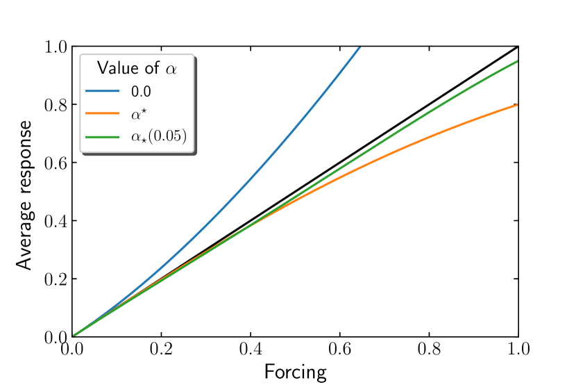
Refer to caption
(a) Full response curves rα(η)subscript𝑟𝛼𝜂r_{\alpha}(\eta) for various α𝛼\alpha.
Refer to caption
(b) Corresponding relative error curves δα(η)subscript𝛿𝛼𝜂\delta_{\alpha}(\eta) relative to the linear response.
Figure 2: Illustration of the effect of different α𝛼\alpha’s on the response

In most practical applications, using α(ε)subscript𝛼𝜀\alpha_{\star}(\varepsilon) is the choice of interest, as the points on the response curve are anyway computed with some numerical error, such as timestep discretization and statistical error. There is, however, a tradeoff to be considered. As one tightens the acceptable relative error by decreasing ε𝜀\varepsilon, the value of ηα(ε)subscript𝜂𝛼𝜀\eta_{\alpha}(\varepsilon) is also decreased. In practice, values of ε𝜀\varepsilon in the range 0.01 to 0.1 are small enough to lead to a bias of a few percent in relative magnitude, but large enough so that the benefit of the increased magnitude of the forcing is significant. We further illustrate the tradeoff in Section 4 with numerical results for several observables for overdamped and underdamped Langevin dynamics.

As a final remark in this section, note that computing α(ε)subscript𝛼𝜀\alpha_{\star}(\varepsilon) requires computing the full response curve. Although this is not practical, the aim here is to provide a proof of principle demonstrating the potential computational gains obtained by making use of synthetic forcings and decide, between various strategies, the most promising one in order to adapt the approach to actual systems of interest.

3.4 Linearly combining extra forcings

As discussed in Section 3.3, with the addition of some extra forcing ~extrasubscript~extra\widetilde{\mathcal{L}}_{\mathrm{extra}}, it is possible to find a value of α𝛼\alpha which cancels the second-order response ρ2subscript𝜌2\rho_{2} due to the linearity of 𝔣2subscript𝔣2\mathfrak{f}_{2} in α𝛼\alpha, as shown in (139). We can extend this notion to linear combinations of extra forcings. In particular, one can combine k𝑘k forcings in order to cancel the first k𝑘k nonlinear orders of the response. That is, for α=(α1,,αk)𝛼subscript𝛼1subscript𝛼𝑘\alpha=(\alpha_{1},\dotsc,\alpha_{k}), the synthetic perturbation ~phys+α1~extra,1++αk~extra,ksubscript~physsubscript𝛼1subscript~extra1subscript𝛼𝑘subscript~extrak\widetilde{\mathcal{L}}_{\mathrm{phys}}+\alpha_{1}\widetilde{\mathcal{L}}_{\mathrm{extra,1}}+\cdots+\alpha_{k}\widetilde{\mathcal{L}}_{\mathrm{extra,k}} can be used, with α𝛼\alpha chosen such that ρ2,α==ρk+1,α=0subscript𝜌2𝛼subscript𝜌𝑘1𝛼0\rho_{2,\alpha}=\cdots=\rho_{k+1,\alpha}=0. This is a nonlinear equation in α𝛼\alpha, with k𝑘k unknowns scalar values and k𝑘k conditions to solve.

4 Numerical results

The aim of the numerical illustrations presented in this section is to demonstrate the potential of the synthetic forcing approach, on the examples given in Section 3.2. The numerical results are obtained by discretizing the PDEs determining the invariant probability measure of each system (namely the Fokker–Planck equation (113)) and the Poisson equation (44). The use of this method, particularly in low-dimensional systems, allows us to extensively and thoroughly examine the quality of synthetic forcings, as we can easily compute full response curves and individual orders of the response, in contrast to Monte Carlo simulations, for which some statistical error and timestep discretization bias are present. This numerical method, however, cannot be used as such for higher dimensional systems, as solving the associated PDEs becomes too cumbersome a task. Thus, for higher dimensional systems, Monte Carlo simulations are usually preferred (see discussion in Section 5).

We first discuss in Section 4.1 the numerical methods used, then present the numerical results for the one and two-dimensional overdamped Langevin, and one-dimensional Langevin dynamics in Sections 4.2, 4.3 and 4.4, respectively. We finally discuss in Section 4.5 the impact of the synthetic forcings approach on variance reduction in the estimation of transport coefficients.

4.1 Numerical method

The full response curve and the linear response are computed by solving the associated Fokker–Planck equation for each dynamics, and the Poisson equation (44), respectively. The main advantage of numerical methods based on solving partial differential equations is that the discretization error can be systematically reduced to a very small value by refining the mesh used to represent the functions at hand. There are two situations in which the solutions to PDEs are required to determine the response to external perturbations, which we outline below.

Approximation of the linear response ρ1subscript𝜌1\rho_{1}

The linear response is obtained by computing 𝔣1subscript𝔣1\mathfrak{f}_{1} and approximating the integral on the right-hand side of (47). To approximate 𝔣1subscript𝔣1\mathfrak{f}_{1}, we solve the Poisson equation (44), which we recall here for convenience:

(149) 0𝔣1=~phys𝟏.superscriptsubscript0subscript𝔣1superscriptsubscript~phys1\mathcal{L}_{0}^{*}\mathfrak{f}_{1}=-\widetilde{\mathcal{L}}_{\mathrm{phys}}^{*}\mathbf{1}.

For overdamped Langevin dynamics, we directly solve (149) as we consider a bounded position space, namely the torus 𝕋dsuperscript𝕋𝑑\mathbb{T}^{d}. For Langevin dynamics, instead of solving for 𝔣1subscript𝔣1\mathfrak{f}_{1} in the expansion (42), we solve for ψ¯1subscript¯𝜓1\overline{\psi}_{1} in ψη=ψ0+ηψ¯1+η2ψ¯2+subscript𝜓𝜂subscript𝜓0𝜂subscript¯𝜓1superscript𝜂2subscript¯𝜓2\psi_{\eta}=\psi_{0}+\eta\overline{\psi}_{1}+\eta^{2}\overline{\psi}_{2}+\cdots, i.e. ψ¯1=𝔣1ψ0subscript¯𝜓1subscript𝔣1subscript𝜓0\overline{\psi}_{1}=\mathfrak{f}_{1}\psi_{0}. This function satisfies the Poisson equation

(150) 0ψ¯1=~physψ0,superscriptsubscript0subscript¯𝜓1superscriptsubscript~physsubscript𝜓0\mathcal{L}_{0}^{\dagger}\overline{\psi}_{1}=-\widetilde{\mathcal{L}}_{\mathrm{phys}}^{\dagger}\psi_{0},

which is equivalent to reformulating (149) in terms of the L2superscript𝐿2L^{2}-adjoint. Due to the unbounded momentum space for Langevin dynamics, solving (150) makes the problem easier to solve numerically than (149). Indeed, the unbounded momentum space needs to be truncated. A natural choice when solving for ψ¯1subscript¯𝜓1\overline{\psi}_{1} is to set Dirichlet boundary conditions at the boundaries of the domain in p𝑝p, which is consistent with the fact that ψ¯1(q,p)subscript¯𝜓1𝑞𝑝\overline{\psi}_{1}(q,p) is expected to vanish as |p|+𝑝|p|\to+\infty. In contrast, there is no natural boundary condition for 𝔣1subscript𝔣1\mathfrak{f}_{1} in (47) when the momentum space is truncated.

Once an approximation of 𝔣1subscript𝔣1\mathfrak{f}_{1} or ψ¯1subscript¯𝜓1\overline{\psi}_{1} is obtained, we perform a quadrature on one of the following integrals to directly find the linear response

(151) ρ1=𝒳R𝔣1ψ0=𝒳Rψ¯1.subscript𝜌1subscript𝒳𝑅subscript𝔣1subscript𝜓0subscript𝒳𝑅subscript¯𝜓1\rho_{1}=\int_{\mathcal{X}}R\mathfrak{f}_{1}\,\psi_{0}=\int_{\mathcal{X}}R\,\overline{\psi}_{1}.

More generally, this procedure can be extended by using the recursive formula (46), which allows for the computation of response terms of arbitrary orders; this is used in particular to compute ρ2,physsubscript𝜌2phys\rho_{2,\text{phys}} and ρ2,extrasubscript𝜌2extra\rho_{2,\text{extra}} when computing the value of αsuperscript𝛼\alpha^{\star} defined in (141).

Approximation of the full response rα(η)subscript𝑟𝛼𝜂r_{\alpha}(\eta)

In this work, we compute the full response in order to quantify how much, and how quickly the response deviates from the linear regime. In actual applications, one typically does not compute the full response curve, in particular when using Monte Carlo simulations. The quantity of interest, namely the transport coefficient, comes from the linear response, which can be obtained from computing a single point (or typically two to ensure linearity), so computing the full response curve is not of interest.

The full response curve can be computed by solving the Fokker–Planck equation (113), which we recall for convenience

(152) η,αψη,α=0,superscriptsubscript𝜂𝛼subscript𝜓𝜂𝛼0\mathcal{L}_{\eta,\alpha}^{\dagger}\psi_{\eta,\alpha}=0,

and then performing a quadrature on the integral

(153) rα(η)=𝒳Rψη,α.subscript𝑟𝛼𝜂subscript𝒳𝑅subscript𝜓𝜂𝛼r_{\alpha}(\eta)=\int_{\mathcal{X}}R\,\psi_{\eta,\alpha}.
Solving the PDE

For the discretization of the PDEs (149), (150) and (152), we use a finite-difference scheme. Periodic boundary conditions are used in the spatial variable since we always consider q𝕋d𝑞superscript𝕋𝑑q\in\mathbb{T}^{d} for both overdamped Lanvegin and Langevin dynamics, with d=1𝑑1d=1 or d=2𝑑2d=2. For overdamped Langevin dynamics, we use a centered finite-difference scheme. For the one-dimensional Langevin dynamics, the momentum variable is first truncated to [pmax,pmax]subscript𝑝maxsubscript𝑝max[-p_{\mathrm{max}},p_{\mathrm{max}}], then its domain is discretized with step size hpsubscript𝑝h_{p}. Dirichlet boundary conditions are imposed at p=±pmax𝑝plus-or-minussubscript𝑝maxp=\pm p_{\mathrm{max}}. We ensured that our truncated value of the momentum pmax=6subscript𝑝max6p_{\mathrm{max}}=6 is large enough so that it does not affect the numerical results. A centered scheme is also used for Langevin dynamics, except for the transport term pTM1qsuperscript𝑝𝑇superscript𝑀1subscript𝑞-p^{T}M^{-1}\nabla_{q} in the Fokker–Planck equation (36), where an upwind scheme is used (refer to Appendix B for the precise expressions of the aforementioned numerical schemes). All computations were performed with the Julia language.

4.2 Overdamped Langevin dynamics - one-dimensional case

We present in this section the numerical results for the one-dimensional overdamped Langevin dynamics (31) on 𝒳=𝕋𝒳𝕋\mathcal{X}=\mathbb{T}, with potential energy

(154) V(q)=cos(2πq).𝑉𝑞2𝜋𝑞V(q)=\cos(2\pi q).

We consider the observable

(155) R(q)=(acos(2πq)+bsin(2πq))eβV(q),𝑅𝑞𝑎2𝜋𝑞𝑏2𝜋𝑞superscripte𝛽𝑉𝑞R(q)=\left(a\cos(2\pi q)+b\sin(2\pi q)\right)\mathrm{e}^{\beta V(q)},

where a,b𝑎𝑏a,b\in\mathbb{R}. We choose this observable for two reasons. First, by construction, it has average zero with respect to the Gibbs probability measure, with density proportional to eβVsuperscripte𝛽𝑉\mathrm{e}^{-\beta V}. Second, we can tune the coefficients a𝑎a and b𝑏b to control the magnitude of the individual orders of response. This allows us to choose a𝑎a and b𝑏b such that the first and second-order responses are normalized, i.e. ρ1=ρ2=1subscript𝜌1subscript𝜌21\rho_{1}=\rho_{2}=1, which makes it easier to compare the quality of each synthetic forcing.

Due to the symmetries of the potential energy function (154), we can directly compute the values of a𝑎a and b𝑏b such that ρ1=ρ2=1subscript𝜌1subscript𝜌21\rho_{1}=\rho_{2}=1. More precisely, it can be shown that 𝔣1subscript𝔣1\mathfrak{f}_{1} and 𝔣2subscript𝔣2\mathfrak{f}_{2} are respectively odd and even on [1/2,1/2]1212[-1/2,1/2] so that b𝑏b controls the magnitude of ρ1subscript𝜌1\rho_{1} and a𝑎a controls the magnitude of ρ2subscript𝜌2\rho_{2}. The value of b𝑏b such that ρ1=1subscript𝜌11\rho_{1}=1 is easily computed using (61) to be

(156) b=(Z1𝒳sin(2πq)𝔣1(q)𝑑q)1,Z=𝒳eV(q)𝑑q.formulae-sequence𝑏superscriptsuperscript𝑍1subscript𝒳2𝜋𝑞subscript𝔣1𝑞differential-d𝑞1𝑍subscript𝒳superscripte𝑉𝑞differential-d𝑞b=\left(Z^{-1}\int_{\mathcal{X}}\sin(2\pi q)\mathfrak{f}_{1}(q)\,dq\right)^{-1},\qquad Z=\int_{\mathcal{X}}\mathrm{e}^{-V(q)}dq.

Similarly, the value of a𝑎a such that ρ2=1subscript𝜌21\rho_{2}=1 is

(157) a=(Z1𝒳cos(2πq)𝔣2(q)𝑑q)1.𝑎superscriptsuperscript𝑍1subscript𝒳2𝜋𝑞subscript𝔣2𝑞differential-d𝑞1a=\left(Z^{-1}\int_{\mathcal{X}}\cos(2\pi q)\mathfrak{f}_{2}(q)\,dq\right)^{-1}.

The spatial domain 𝕋=[0,1)𝕋01\mathbb{T}=[0,1) is discretized into m=2000𝑚2000m=2000 points, with uniform step size h=1/m1𝑚h=1/m. The simulations were performed with inverse temperature β=1𝛽1\beta=1 and mass M=1𝑀1M=1, which is also the setting for the results in two dimensions obtained in Section 4.3. Moreover, we consider the forcing F=1𝐹1F=1, as this is the only nongradient forcing in dimension one on the torus.

We present the full response curves and the associated linear response for each of the three synthetic forcings discussed in Section 3.2.2. Figures 3(a), 3(b) and 3(c) correspond to the Feynman–Kac forcing (124), modified fluctuation-dissipation (121) and divergence-free vector field (116), respectively. Note that in dimension one, (116) reduces to a single option, namely

(158) ~extra=eVddq,subscript~extrasuperscripte𝑉𝑑𝑑𝑞\widetilde{\mathcal{L}}_{\mathrm{extra}}=\mathrm{e}^{V}\frac{d}{dq},

which is the one used here. For each of the plots, we show the linear response, the full response curve r0(η)subscript𝑟0𝜂r_{0}(\eta) for α=0𝛼0\alpha=0, the response curve for rα(η)subscript𝑟superscript𝛼𝜂r_{\alpha^{\star}}(\eta) for αsuperscript𝛼\alpha^{\star} computed using (141), and response curves for some additional values of α𝛼\alpha\in\mathbb{R} for illustrative purposes. In some cases, in particular when the response curve associated with αsuperscript𝛼\alpha^{\star} sees marginal improvement in extending the linear regime, we also compute the curve for α(ε)subscript𝛼𝜀\alpha_{\star}(\varepsilon), where we choose ε=0.05𝜀0.05\varepsilon=0.05. Lastly, Figure 3(d) includes all synthetic forcings. Note that the maximal value of the forcing is much larger for Figure 3(d), where we compare the best choices for the magnitude of each synthetic forcing; this is also the setting for the illustrations presented in Sections 4.3 and 4.4.
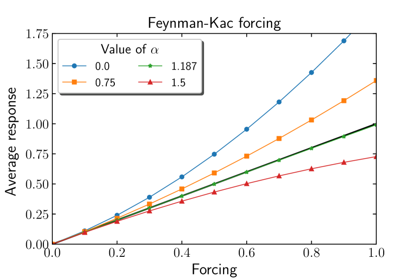
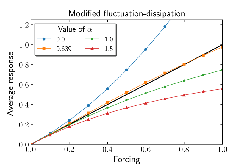
Refer to caption
(a) Feynman–Kac forcing, α=1.187superscript𝛼1.187\alpha^{\star}=1.187.
Refer to caption
(b) Modified FD, α=1.0superscript𝛼1.0\alpha^{\star}=1.0.
Refer to caption
(c) Div-free vector field, α=0.835superscript𝛼0.835\alpha^{\star}=-0.835.
Refer to caption
(d) Comparing αsuperscript𝛼\alpha^{\star} for all forcings.
Figure 3: Response curves for various synthetic forcings for the one-dimensional overdamped Langevin dynamics.

The choice αsuperscript𝛼\alpha^{\star}, namely the one that cancels the second order response ρ2subscript𝜌2\rho_{2}, performs quite well for the Feynman–Kac and divergence-free forcings, as seen in Figures 3(a) and 3(c). It allows to extend the range of linearity for η>1𝜂1\eta>1, an increase of over tenfold when compared to the original response curve for α=0𝛼0\alpha=0. This allows for a variance reduction of a factor of order 1000 for the estimator (69), as documented in Section 4.5.

Figure 3(b) illustrates the discussion of Section 3.3 about choosing the values of α𝛼\alpha allowing to stay longer in an approximate linear response. Although the value of the parameter α𝛼\alpha such that ρ2(α)=0subscript𝜌2𝛼0\rho_{2}(\alpha)=0 is α=1.0superscript𝛼1.0\alpha^{\star}=1.0 for the modified fluctuation-dissipation, we see that α(0.05)=0.639subscript𝛼0.050.639\alpha_{\star}(0.05)=0.639 is a much more nicely behaved curve, staying within 5% relative error for a large η𝜂\eta regime. This is a consequence of the fact that although αsuperscript𝛼\alpha^{\star} cancels ρ2subscript𝜌2\rho_{2}, it might significantly increase ρ3subscript𝜌3\rho_{3} and higher order terms.

4.3 Overdamped Langevin dynamics - two-dimensional case

We now present the numerical results for overdamped Langevin dynamics in dimension two, defined on 𝒳=𝕋2𝒳superscript𝕋2\mathcal{X}=\mathbb{T}^{2}, with the following periodic potential energy:

(159) V(q)=12cos(2πq1)+cos(2πq2)+κcos(2π(q1q2)),𝑉𝑞122𝜋subscript𝑞12𝜋subscript𝑞2𝜅2𝜋subscript𝑞1subscript𝑞2V(q)=\frac{1}{2}\cos(2\pi q_{1})+\cos(2\pi q_{2})+\kappa\cos\left(2\pi(q_{1}-q_{2})\right),

with κ𝜅\kappa\in\mathbb{R}. The observable considered here is of the same form as (155), and reads

(160) R(q)=(acos(2πq1)+bsin(2πq1))eβV(q).𝑅𝑞𝑎2𝜋subscript𝑞1𝑏2𝜋subscript𝑞1superscripte𝛽𝑉𝑞R(q)=\left(a\cos(2\pi q_{1})+b\sin(2\pi q_{1})\right)\mathrm{e}^{\beta V(q)}.

For observables of this form, expressions (156) and (157) can be generalized to higher dimensions to compute the normalization constants. As in Section 4.2, this ensures that ρ1=ρ2=1subscript𝜌1subscript𝜌21\rho_{1}=\rho_{2}=1 when κ=0𝜅0\kappa=0. When κ𝜅\kappa is nonzero but not too large, ρ1subscript𝜌1\rho_{1} and ρ2subscript𝜌2\rho_{2} are of order 1, which is convenient to observe deviations from the linear regime.

For all numerical results presented here, we considered κ=0.3𝜅0.3\kappa=0.3 and a constant nongradient forcing F=(1,0)2𝐹10superscript2F=(1,0)\in\mathbb{R}^{2}. The spatial domain 𝕋2=[0,1)2superscript𝕋2superscript012\mathbb{T}^{2}=[0,1)^{2} was discretized using a regular product mesh of mq=200subscript𝑚𝑞200m_{q}=200 points per dimension.

Refer to caption
(a) Feynman–Kac forcing, α=1.035subscript𝛼1.035\alpha_{\star}=1.035.
Refer to caption
(b) Modified FD, α=1.301subscript𝛼1.301\alpha_{\star}=1.301.
Refer to caption
(c) Div-free vector field eVsuperscripte𝑉\mathrm{e}^{V}, α=0.878subscript𝛼0.878\alpha_{\star}=-0.878.
Refer to caption
(d) Div-free vector field AV𝐴𝑉A\nabla V, α=6.11subscript𝛼6.11\alpha_{\star}=6.11.
Refer to caption
(e) All forcings.
Figure 4: Response curves for various synthetic forcings for the two-dimensional overdamped Langevin dynamics.

The results presented in Figure 4 correspond to response curves for each of the synthetic forcings discussed in Section 3.2.2. Figure 4(a) corresponds to the Feynman–Kac forcing (124), with ξ=(1,0)2𝜉10superscript2\xi=(1,0)\in\mathbb{R}^{2}. It is observed that this extra forcing is more effective in extending the linear regime when it is in the same direction as the physical perturbation F𝐹F, hence our choice of ξ𝜉\xi. We generalize the exponential divergence-free vector field (158) presented in Section 4.2 to higher dimensions as ~extra=eV()\widetilde{\mathcal{L}}_{\mathrm{extra}}=\mathrm{e}^{V}(\nabla\cdot), presented in Figure 4(c).

Overall, the results are qualitatively similar to those from Section 4.2, apart from two main differences. First, we present a divergence-free vector field of the form VTAsuperscript𝑉𝑇𝐴\nabla V^{T}A\nabla, with A𝐴A the symplectic matrix given by (128), which has an underwhelming impact on increasing the linear regime as seen in Figure 4(d), even for α(0.05)=2.0subscript𝛼0.052.0\alpha_{\star}(0.05)=2.0. It seems therefore not to be a good option to consider. Second, Figure 4(e) shows that the Feynman–Kac forcing performs better than the exponential divergence-free field. On the other hand, the modified fluctuation-dissipation (121) is once again underwhelming, as seen in Figure 4(b), with response curve for α(0.05)=0.59subscript𝛼0.050.59\alpha_{\star}(0.05)=0.59 once again performing better than α=1.301superscript𝛼1.301\alpha^{\star}=1.301. Note that the value α(ε)subscript𝛼𝜀\alpha_{\star}(\varepsilon) was not computed for the Feynman–Kac and the exponential divergence-free forcings, as αsuperscript𝛼\alpha^{\star} sufficiently extends the regime of linear response for those cases.

4.4 Langevin dynamics - one-dimensional case

We present here the numerical results associated with the one-dimensional Langevin dynamics (38), where the potential energy function is the same as the one used for the one-dimensional overdamped Langevin dynamics case, namely (154), and the same observable (155) as in Section 4.2. The normalization constants a𝑎a and b𝑏b for ρ1subscript𝜌1\rho_{1} and ρ2subscript𝜌2\rho_{2} are chosen to be

(161) b=(1Z2π/β𝒳×dsin(2πq)𝔣1(q,p)exp(βp2/2)𝑑p𝑑q)1,𝑏superscript1𝑍2𝜋𝛽subscript𝒳superscript𝑑2𝜋𝑞subscript𝔣1𝑞𝑝𝛽superscript𝑝22differential-d𝑝differential-d𝑞1b=\left(\frac{1}{Z\sqrt{2\pi/\beta}}\int_{\mathcal{X}\times\mathbb{R}^{d}}\sin(2\pi q)\mathfrak{f}_{1}(q,p)\exp(-\beta p^{2}/2)dp\,dq\right)^{-1},
(162) a=(1Z2π/β𝒳×dcos(2πq)𝔣2(q,p)exp(βp2/2)𝑑p𝑑q)1,𝑎superscript1𝑍2𝜋𝛽subscript𝒳superscript𝑑2𝜋𝑞subscript𝔣2𝑞𝑝𝛽superscript𝑝22differential-d𝑝differential-d𝑞1a=\left(\frac{1}{Z\sqrt{2\pi/\beta}}\int_{\mathcal{X}\times\mathbb{R}^{d}}\cos(2\pi q)\mathfrak{f}_{2}(q,p)\exp(-\beta p^{2}/2)dp\,dq\right)^{-1},

with Z𝑍Z the same normalization constant as in Section 4.2, defined in (156). The spatial domain 𝕋=[0,1)𝕋01\mathbb{T}=[0,1) was discretized using mq=200subscript𝑚𝑞200m_{q}=200 points, with uniform step size hq=1/mqsubscript𝑞1subscript𝑚𝑞h_{q}=1/m_{q}. The unbounded momentum space was truncated to [pmax,pmax]subscript𝑝maxsubscript𝑝max[-p_{\mathrm{max}},p_{\mathrm{max}}] with pmax=6.0subscript𝑝max6.0p_{\mathrm{max}}=6.0, with Dirichlet boundary conditions at p=±pmax𝑝plus-or-minussubscript𝑝maxp=\pm p_{\mathrm{max}}, and then discretized into mp=1000subscript𝑚𝑝1000m_{p}=1000 points with uniform step size hp=2pmax/(mp1)subscript𝑝2subscript𝑝maxsubscript𝑚𝑝1h_{p}=2p_{\mathrm{max}}/(m_{p}-1). The simulations were performed with β=γ=M=1𝛽𝛾𝑀1\beta=\gamma=M=1. Note that when computing the response associated with the divergence-free vector field for large values of η𝜂\eta, as presented in Figure 5(e), the momentum space is truncated to pmax=10subscript𝑝max10p_{\mathrm{max}}=10.

The results presented in Figure 5 correspond to the response curves for each of the synthetic forcings discussed in Section 3.2.3. Figures 5(a) and 5(b) correspond to the position and momentum components of the modified fluctuation-dissipation forcing presented in Example 3.5, respectively, namely

(163) ~extra=qq,~extra=pp.formulae-sequencesubscript~extrasuperscriptsubscript𝑞subscript𝑞subscript~extrasuperscriptsubscript𝑝subscript𝑝\widetilde{\mathcal{L}}_{\mathrm{extra}}=-\partial_{q}^{*}\partial_{q},\qquad\widetilde{\mathcal{L}}_{\mathrm{extra}}=-\partial_{p}^{*}\partial_{p}.

Figures 5(c) and 5(d) correspond to the position and momentum components of the Feynman–Kac forcing presented in Example 3.6, respectively, namely

(164) ~extra=q=Vq,~extra=p=pp.formulae-sequencesubscript~extrasuperscriptsubscript𝑞superscript𝑉subscript𝑞subscript~extrasuperscriptsubscript𝑝𝑝subscript𝑝\widetilde{\mathcal{L}}_{\mathrm{extra}}=\partial_{q}^{*}=V^{\prime}-\partial_{q},\qquad\widetilde{\mathcal{L}}_{\mathrm{extra}}=\partial_{p}^{*}=p-\partial_{p}.

Lastly, Figure 5(e) corresponds to the divergence-free forcing (158).
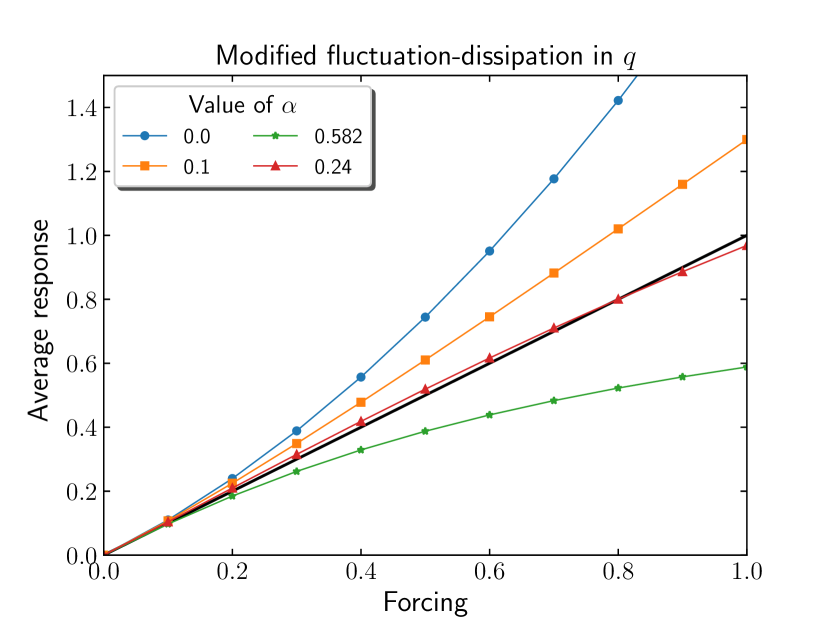
Refer to caption
(a) Modified FD in q𝑞q, α=0.582subscript𝛼0.582\alpha_{\star}=0.582.
Refer to caption
(b) Modified FD in p𝑝p, α=5.640subscript𝛼5.640\alpha_{\star}=5.640.
Refer to caption
(c) Feynman–Kac forcing in q𝑞q, α=0.268subscript𝛼0.268\alpha_{\star}=0.268.
Refer to caption
(d) Feynman–Kac forcing in p𝑝p, α=0.528subscript𝛼0.528\alpha_{\star}=-0.528.
Refer to caption
(e) Div-free vector field, α=0.2subscript𝛼0.2\alpha_{\star}=-0.2.
Refer to caption
(f) All forcings.
Figure 5: Response curves for various synthetic forcings for the one-dimensional Langevin dynamics.

For both modified fluctuation-dissipation forcings, Figures 5(a) and 5(b), we see that αsuperscript𝛼\alpha^{\star} does not preserve linearity for a large η𝜂\eta regime, suggesting instead that α(ε)subscript𝛼𝜀\alpha_{\star}(\varepsilon) is the better choice for practical applications; the same conclusion was drawn for the modified fluctuation-dissipation forcing for overdamped Langevin in Section 4.2. Among the two forcings, it seems better to modify the fluctuation-dissipation in p𝑝p as the response remains longer in the linear response regime for the optimal value α(ε)subscript𝛼𝜀\alpha_{\star}(\varepsilon).

Both Feynman–Kac forcings showcase great potential in extending the linear regime. Once again, Figures 5(d) and 5(f) suggest that opting for the extra forcing in the p𝑝p variable is the superior choice.

Lastly, the divergence-free forcing greatly increases the linear regime, as seen in Figures 5(e) and 5(f). This behavior, as well as the ease to implement it in Monte Carlo simulations, make it is the most appealing choice of forcing, allowing to substantially reduce the variance of the estimator (69), as discussed in Section 4.5. Although the Feynman–Kac extra forcing also demonstrates great potential in extending the linear regime, the challenges associated with its implementation render it an impractical choice.

4.5 Scaling of the variance

We discuss in this section the scaling of the variance σR,η2/η2subscriptsuperscript𝜎2𝑅𝜂superscript𝜂2\sigma^{2}_{R,\eta}/\eta^{2}, defined in (82), with the addition of synthetic forces, and in particular numerically illustrate the potential of synthetic forcings as a tool for variance reduction. See Appendix B for details on the numerical computation of (82). We emphasize that the bias on the estimator (69), made precise in (79), is negligible when compared to the variance, hence we concentrate on the variance. We anyway want to remain in the linear response regime so, by construction, the bias should be small.

Recall from Section 2.3, and in particular in Proposition 2.5, that the estimator Φ^η,tsubscript^Φ𝜂𝑡\widehat{\Phi}_{\eta,t} defined in (69) has asymptotic variance of order σR,η2/η2subscriptsuperscript𝜎2𝑅𝜂superscript𝜂2\sigma^{2}_{R,\eta}/\eta^{2}. Indeed, (81) suggests that this asymptotic variance is of the same order as the one associated with the equilibrium estimator, i.e. σR,02/η2subscriptsuperscript𝜎2𝑅0superscript𝜂2\sigma^{2}_{R,0}/\eta^{2}, up to a small bias of order η𝜂\eta:

(165) σR,η2η2=σR,02η2+O(1η).subscriptsuperscript𝜎2𝑅𝜂superscript𝜂2subscriptsuperscript𝜎2𝑅0superscript𝜂2O1𝜂\frac{\sigma^{2}_{R,\eta}}{\eta^{2}}=\frac{\sigma^{2}_{R,0}}{\eta^{2}}+\mathrm{O}\left(\frac{1}{\eta}\right).

This suggests that the asymptotic variance σR,η2subscriptsuperscript𝜎2𝑅𝜂\sigma^{2}_{R,\eta} has sufficiently small variations in η𝜂\eta, which validates increasing η𝜂\eta as a way to substantially reduce the variance.

For each synthetic forcing and a fixed value of α𝛼\alpha, we compute σR,η2/η2subscriptsuperscript𝜎2𝑅𝜂superscript𝜂2\sigma^{2}_{R,\eta}/\eta^{2} with η=ηα(ε)𝜂subscript𝜂𝛼𝜀\eta=\eta_{\alpha}(\varepsilon) defined in (147), i.e. the first value of η𝜂\eta at which the response curve departs ε𝜀\varepsilon in relative error relative to the linear response. For the results here presented, we use ε=0.05𝜀0.05\varepsilon=0.05. For each of the dynamics, the scaled asymptotic variance as a function of η𝜂\eta is illustrated in Figure 6, where the values of ηα(ε)subscript𝜂𝛼𝜀\eta_{\alpha}(\varepsilon) are represented as dashed vertical lines to highlight the great reduction in variance potential. As expected, Figure 6 is consistent with (165), and it shows that increasing the regime of linear response has a dramatic effect on the variance.

In order to quantity the variance reduction, we define the gain as the ratio of the variance of the equilibrium system and its synthetic counterpart:

(166) gain=(σR,η0(ε)2η0(ε)2)(σR,ηα(ε)2ηα(ε)2)1.gainsubscriptsuperscript𝜎2𝑅subscript𝜂0𝜀subscript𝜂0superscript𝜀2superscriptsubscriptsuperscript𝜎2𝑅subscript𝜂𝛼𝜀subscript𝜂𝛼superscript𝜀21\mathrm{gain}=\left(\frac{\sigma^{2}_{R,\eta_{0}(\varepsilon)}}{\eta_{0}(\varepsilon)^{2}}\right)\left(\frac{\sigma^{2}_{R,\eta_{\alpha}(\varepsilon)}}{\eta_{\alpha}(\varepsilon)^{2}}\right)^{-1}.

For each of the cases presented in Table 1, namely the modified-fluctuation dissipation (MFD), Feynman–Kac forcing (FK) and divergence-free vector field (DF), α𝛼\alpha is chosen to be αsuperscript𝛼\alpha^{\star} or α(ε)subscript𝛼𝜀\alpha_{\star}(\varepsilon), and the associated quantity ηα(ε)subscript𝜂𝛼𝜀\eta_{\alpha}(\varepsilon) is computed, where η0(ε)=0.05subscript𝜂0𝜀0.05\eta_{0}(\varepsilon)=0.05 for all three dynamics. Note that for Langevin dynamics, the results here presented for the modified fluctuation-dissipation and the Feynman–Kac forcing both correspond to their p𝑝p counterparts.

Refer to caption
(a) Overdamped Langevin dynamics in 1D.
Refer to caption
(b) Overdamped Langevin dynamics in 2D.
Refer to caption
(c) Langevin dynamics in 1D.
Figure 6: Scaled asymptotic variance σR,η2/η2subscriptsuperscript𝜎2𝑅𝜂superscript𝜂2\sigma^{2}_{R,\eta}/\eta^{2} as a function of η𝜂\eta for various synthetic forcings for all dynamics.
Dynamics Extra forcing
none MFD FK DF (eVsuperscripte𝑉\mathrm{e}^{V}) DF (AV𝐴𝑉A\nabla V)
Ovd. 1D 1 6.56×1026.56superscript102{6.56}\times 10^{2} 1.58×1031.58superscript103{1.58}\times 10^{3} 1.28×1051.28superscript105{1.28}\times 10^{5} -
Ovd. 2D 1 7.65×1027.65superscript102{7.65}\times 10^{2} 3.23×1043.23superscript104{3.23}\times 10^{4} 3.33×1033.33superscript103{3.33}\times 10^{3} 4.03×1004.03superscript100{4.03}\times 10^{0}
Lang. 1D 1 2.18×1032.18superscript103{2.18}\times 10^{3} 1.29×1031.29superscript103{1.29}\times 10^{3} 1.42×1031.42superscript103{1.42}\times 10^{3} -
Table 1: Impact of synthetic forcings on variance reduction: gain (166) for various synthetic forcings for each dynamics.

The results in Table 1 show that the variance can be dramatically reduced with the use of synthetic forcings. Although no choice of extra forcing is universally better, we can achieve reduce the variance by a factor of over 100010001000 in all cases.

5 Extensions and perspectives

Let us conclude this work by discussing potential extensions of our approach and practical applications to real molecular dynamics systems. The notion of synthetic forcings, as here presented, can be applied to a number of actual systems to assist in the computation of transport coefficients, e.g. Lennard–Jones fluids for the computation of shear viscosity, or systems of atom chains for the computation of thermal transport (see [32, 8, 31]).

The methodology here presented, however, must undergo some adaptation to be applied to actual systems. The numerical method we rely on, namely discretizing and solving the associated PDEs, does not scale well to higher dimensions and thus cannot be used as such. One typically relies on Monte Carlo simulations, which normally limits the number of values of η𝜂\eta used due to the high computational cost. Additionally, the computation of the optimal values of α𝛼\alpha, presented in Section 3.3, also cannot be done as such, as it relies on either the PDE approach, or the computation of full response curves.

One preliminary idea for the computation of α𝛼\alpha in real systems is the notion of prescreening. Transport coefficients are intensive quantities, i.e. they do not depend too drastically on the system size. This suggests, in practice, that one performs two simulations with small system sizes, with α1α2subscript𝛼1subscript𝛼2\alpha_{1}\neq\alpha_{2}, from which the value of αsuperscript𝛼\alpha^{\star} can be extrapolated, which can then be used in a large scale simulation. The results here presented suggest that such an adaptation, which is work in progress, is worth the effort.

Appendix A Analysis of eigenvalues for Feynman–Kac forcings

As discussed in Section 3.2.1, the operator η,α=0+η(~phys+α~extra)subscript𝜂𝛼subscript0𝜂subscript~phys𝛼subscript~extra\mathcal{L}_{\eta,\alpha}=\mathcal{L}_{0}+\eta(\widetilde{\mathcal{L}}_{\mathrm{phys}}+\alpha\widetilde{\mathcal{L}}_{\mathrm{extra}}) admits a nonzero principal eigenvalue λη,αsubscript𝜆𝜂𝛼\lambda_{\eta,\alpha} when ~extrasubscript~extra\widetilde{\mathcal{L}}_{\mathrm{extra}} corresponds to the Feynman–Kac forcing, discussed in Examples 3.3 and 3.6. As a consequence, the Poisson equation (46) must be reformulated for such operators. In this section, we start by formally showing that λη,αsubscript𝜆𝜂𝛼\lambda_{\eta,\alpha} is of order η2superscript𝜂2\eta^{2}, then we discuss the reformulation of (46), in particular to compute αsuperscript𝛼\alpha^{\star}. This analysis could be made precise by adapting the approach of [16].

Quantifying the magnitude of λη,αsubscript𝜆𝜂𝛼\lambda_{\eta,\alpha}

For a general perturbed dynamics, we write the generator η,αsubscript𝜂𝛼\mathcal{L}_{\eta,\alpha} as η,α=0+η(~phys+α~extra)subscript𝜂𝛼subscript0𝜂subscript~phys𝛼subscript~extra\mathcal{L}_{\eta,\alpha}=\mathcal{L}_{0}+\eta(\widetilde{\mathcal{L}}_{\mathrm{phys}}+\alpha\widetilde{\mathcal{L}}_{\mathrm{extra}}), with ~extra=ξTsubscript~extrasuperscript𝜉𝑇superscript\widetilde{\mathcal{L}}_{\mathrm{extra}}=\xi^{T}\nabla^{*} for Feynman–Kac forcings. The associated Fokker–Planck equation is then

(167) (0+η~phys+αη~extra)ψη,α=λη,αψη,α.superscriptsubscript0𝜂subscript~phys𝛼𝜂subscript~extrasubscript𝜓𝜂𝛼subscript𝜆𝜂𝛼subscript𝜓𝜂𝛼\left(\mathcal{L}_{0}+\eta\widetilde{\mathcal{L}}_{\mathrm{phys}}+\alpha\eta\widetilde{\mathcal{L}}_{\mathrm{extra}}\right)^{\dagger}\psi_{\eta,\alpha}=\lambda_{\eta,\alpha}\psi_{\eta,\alpha}.

For a fixed value of α𝛼\alpha, formally expanding ψη,αsubscript𝜓𝜂𝛼\psi_{\eta,\alpha} and λη,αsubscript𝜆𝜂𝛼\lambda_{\eta,\alpha} in powers of η𝜂\eta yields

(168) ψη=ψ0+ηψ¯1+η2ψ¯2,α+,λη,α=ηλ¯1,α+η2λ¯2,α+.formulae-sequencesubscript𝜓𝜂subscript𝜓0𝜂subscript¯𝜓1superscript𝜂2subscript¯𝜓2𝛼subscript𝜆𝜂𝛼𝜂subscript¯𝜆1𝛼superscript𝜂2subscript¯𝜆2𝛼\psi_{\eta}=\psi_{0}+\eta\overline{\psi}_{1}+\eta^{2}\overline{\psi}_{2,\alpha}+\cdots,\qquad\lambda_{\eta,\alpha}=\eta\overline{\lambda}_{1,\alpha}+\eta^{2}\overline{\lambda}_{2,\alpha}+\cdots.

Note that ψ¯1subscript¯𝜓1\overline{\psi}_{1} has no α𝛼\alpha dependency, since the addition of α~extra𝛼subscript~extra\alpha\widetilde{\mathcal{L}}_{\mathrm{extra}} leaves 𝔣1subscript𝔣1\mathfrak{f}_{1} invariant due to (112), as discussed in Section 3.1.

We substitute the expansions (168) in the Fokker–Planck equation (167). Identifying terms with the same orders in η𝜂\eta leads to

(169) O(η)::O𝜂absent\displaystyle\mathrm{O}(\eta): 0ψ¯1+(~phys+α~extra)ψ0λ¯1,αψ0=0,superscriptsubscript0subscript¯𝜓1superscriptsubscript~phys𝛼superscriptsubscript~extrasubscript𝜓0subscript¯𝜆1𝛼subscript𝜓00\displaystyle\quad\mathcal{L}_{0}^{\dagger}\overline{\psi}_{1}+\left(\widetilde{\mathcal{L}}_{\mathrm{phys}}^{\dagger}+\alpha\widetilde{\mathcal{L}}_{\mathrm{extra}}^{\dagger}\right)\psi_{0}-\overline{\lambda}_{1,\alpha}\psi_{0}=0,
(170) O(η2)::Osuperscript𝜂2absent\displaystyle\mathrm{O}(\eta^{2}): 0ψ¯2,α+(~phys+α~extra)ψ¯1λ¯1,αψ¯1λ¯2,αψ0=0.superscriptsubscript0subscript¯𝜓2𝛼superscriptsubscript~phys𝛼superscriptsubscript~extrasubscript¯𝜓1subscript¯𝜆1𝛼subscript¯𝜓1subscript¯𝜆2𝛼subscript𝜓00\displaystyle\quad\mathcal{L}_{0}^{\dagger}\overline{\psi}_{2,\alpha}+\left(\widetilde{\mathcal{L}}_{\mathrm{phys}}^{\dagger}+\alpha\widetilde{\mathcal{L}}_{\mathrm{extra}}^{\dagger}\right)\overline{\psi}_{1}-\overline{\lambda}_{1,\alpha}\overline{\psi}_{1}-\overline{\lambda}_{2,\alpha}\psi_{0}=0.

From the O(η)O𝜂\mathrm{O}(\eta) expression, an integration leads to

(171) λ¯1,α𝒳ψ0=𝒳0ψ¯1+𝒳~physψ0+α𝒳~extraψ0.subscript¯𝜆1𝛼subscript𝒳subscript𝜓0subscript𝒳superscriptsubscript0subscript¯𝜓1subscript𝒳superscriptsubscript~physsubscript𝜓0𝛼subscript𝒳superscriptsubscript~extrasubscript𝜓0\overline{\lambda}_{1,\alpha}\int_{\mathcal{X}}\psi_{0}=\int_{\mathcal{X}}\mathcal{L}_{0}^{\dagger}\,\overline{\psi}_{1}+\int_{\mathcal{X}}\widetilde{\mathcal{L}}_{\mathrm{phys}}^{\dagger}\psi_{0}+\alpha\int_{\mathcal{X}}\widetilde{\mathcal{L}}_{\mathrm{extra}}^{\dagger}\,\psi_{0}.

From the definition of the L2superscript𝐿2L^{2}-adjoint, it follows that the first two terms on the right-hand side of (171) are 0, since 0𝟏=~phys𝟏=0subscript01subscript~phys10\mathcal{L}_{0}\mathbf{1}=\widetilde{\mathcal{L}}_{\mathrm{phys}}\mathbf{1}=0. The remaining term can be written as

(172) 𝒳~extraψ0=𝒳(~extra𝟏)ψ0=𝒳(ξT𝟏)ψ0=𝒳ξT𝟏ψ0=0.subscript𝒳superscriptsubscript~extrasubscript𝜓0subscript𝒳subscript~extra1subscript𝜓0subscript𝒳superscript𝜉𝑇superscript1subscript𝜓0subscript𝒳superscript𝜉𝑇1subscript𝜓00\int_{\mathcal{X}}\widetilde{\mathcal{L}}_{\mathrm{extra}}^{\dagger}\,\psi_{0}=\int_{\mathcal{X}}\left(\widetilde{\mathcal{L}}_{\mathrm{extra}}\mathbf{1}\right)\psi_{0}=\int_{\mathcal{X}}\left(\xi^{T}\nabla^{*}\mathbf{1}\right)\psi_{0}=\int_{\mathcal{X}}\xi^{T}\nabla\mathbf{1}\,\psi_{0}=0.

Thus, we conclude that λ¯1,α=0subscript¯𝜆1𝛼0\overline{\lambda}_{1,\alpha}=0. Similarly, integrating (170) on 𝒳𝒳\mathcal{X} leads to

(173) λ¯2,α=α𝒳~extraψ¯1=α𝒳(~extra𝟏)ψ¯1,subscript¯𝜆2𝛼𝛼subscript𝒳superscriptsubscript~extrasubscript¯𝜓1𝛼subscript𝒳subscript~extra1subscript¯𝜓1\overline{\lambda}_{2,\alpha}=\alpha\int_{\mathcal{X}}\widetilde{\mathcal{L}}_{\mathrm{extra}}^{\dagger}\,\overline{\psi}_{1}=\alpha\int_{\mathcal{X}}\left(\widetilde{\mathcal{L}}_{\mathrm{extra}}\mathbf{1}\right)\overline{\psi}_{1},

which is generally a nonzero quantity. This suggests that

(174) λη,α=αη2𝒳(~extra𝟏)ψ¯1+O(η3).subscript𝜆𝜂𝛼𝛼superscript𝜂2subscript𝒳subscript~extra1subscript¯𝜓1Osuperscript𝜂3\lambda_{\eta,\alpha}=\alpha\eta^{2}\int_{\mathcal{X}}\left(\widetilde{\mathcal{L}}_{\mathrm{extra}}\mathbf{1}\right)\overline{\psi}_{1}+\mathrm{O}(\eta^{3}).
Reformulating the Poisson equation

Computing the optimal value αsuperscript𝛼\alpha^{\star} defined in (141) requires computing the second-order response, as discussed in Section 3.3. In particular, this is done by using the recursive expression (46), obtained from the Fokker–Planck equation via formal asymptotics. We reformulate (46) for Feynman–Kac systems to compute the second-order response, using that, in view of (170),

(175) ψ¯2,α=(01)[(~phys+α~extra)ψ¯1λ¯2,αψ0],subscript¯𝜓2𝛼superscriptsuperscriptsubscript01delimited-[]superscriptsubscript~phys𝛼superscriptsubscript~extrasubscript¯𝜓1subscript¯𝜆2𝛼subscript𝜓0\overline{\psi}_{2,\alpha}=\left(-\mathcal{L}_{0}^{-1}\right)^{\dagger}\left[\left(\widetilde{\mathcal{L}}_{\mathrm{phys}}^{\dagger}+\alpha\widetilde{\mathcal{L}}_{\mathrm{extra}}^{\dagger}\right)\overline{\psi}_{1}-\overline{\lambda}_{2,\alpha}\psi_{0}\right],

where the value of λ¯2,αsubscript¯𝜆2𝛼\overline{\lambda}_{2,\alpha} is determined by (173). This procedure could be extended to arbitrary orders by identifying terms with the same orders in η𝜂\eta in (167).

Appendix B Numerical scheme for finite differences

We describe here the numerical schemes used to discretize Fokker–Planck equations, used to solve for the density of the invariant probability measure for the systems at hand, namely overdamped Langevin dynamics in one and two dimensions, and Langevin dynamics in one dimension. This approach can be straightforwardly extended to solving Poisson equations with nontrivial right-hand sides such as (44) or the integrand in the asymptotic variance (82). We start each section by first discussing the discretizations associated with the equilibrium dynamics, after which we mention the modification needed when adding perturbations.

For all systems, the spatial domain, namely the torus 𝕋d=[0,1)dsuperscript𝕋𝑑superscript01𝑑\mathbb{T}^{d}=[0,1)^{d}, is discretized into mqdsuperscriptsubscript𝑚𝑞𝑑m_{q}^{d} points with uniform step size hq=1/mqsubscript𝑞1subscript𝑚𝑞h_{q}=1/m_{q} in each direction. While ψηsubscript𝜓𝜂\psi_{\eta} denotes the invariant measure at the continuous level, we use ΨηhsuperscriptsubscriptΨ𝜂\Psi_{\eta}^{h} to denote its discretized counterpart, namely the approximations of the values of ψηsubscript𝜓𝜂\psi_{\eta} at the grid points.

B.1 Overdamped Langevin dynamics

For a continuous function u:𝕋:𝑢𝕋u\colon\mathbb{T}\to\mathbb{R}, we denote by [u]i=u(Qi)subscriptdelimited-[]𝑢𝑖𝑢subscript𝑄𝑖[u]_{i}=u(Q_{i}), where Qi=ihqsubscript𝑄𝑖𝑖subscript𝑞Q_{i}=ih_{q} are the mesh points. Similarly, for a continuous function u:𝕋2:𝑢superscript𝕋2u\colon\mathbb{T}^{2}\to\mathbb{R}, we denote by [u]i,j=u(Qi,j)subscriptdelimited-[]𝑢𝑖𝑗𝑢subscript𝑄𝑖𝑗[u]_{i,j}=u(Q_{i,j}), where Qi,j=(ihq,jhq)subscript𝑄𝑖𝑗𝑖subscript𝑞𝑗subscript𝑞Q_{i,j}=(ih_{q},jh_{q}) are the mesh points. The Fokker–Planck equation to discretize for the overdamped Langevin dynamics (27) reads

(176) 0ψ0=div(Vψ0)+1βΔψ0=VTψ0+ΔVψ0+1βΔψ0.superscriptsubscript0subscript𝜓0div𝑉subscript𝜓01𝛽Δsubscript𝜓0superscript𝑉𝑇subscript𝜓0Δ𝑉subscript𝜓01𝛽Δsubscript𝜓0\mathcal{L}_{0}^{\dagger}\psi_{0}=\operatorname{div}(\nabla V\psi_{0})+\frac{1}{\beta}\Delta\psi_{0}=\nabla V^{T}\nabla\psi_{0}+\Delta V\psi_{0}+\frac{1}{\beta}\Delta\psi_{0}.

Using centered finite differences, the discretization of (176) in dimension one is given by

(177) [V]i[Ψ0h]i+1[Ψ0h]i12hq+[V′′]i[Ψ0h]i+[Ψ0h]i+12[Ψ0h]i+[Ψ0h]i1βhq2=0.subscriptdelimited-[]superscript𝑉𝑖subscriptdelimited-[]subscriptsuperscriptΨ0𝑖1subscriptdelimited-[]subscriptsuperscriptΨ0𝑖12subscript𝑞subscriptdelimited-[]superscript𝑉′′𝑖subscriptdelimited-[]subscriptsuperscriptΨ0𝑖subscriptdelimited-[]subscriptsuperscriptΨ0𝑖12subscriptdelimited-[]subscriptsuperscriptΨ0𝑖subscriptdelimited-[]subscriptsuperscriptΨ0𝑖1𝛽superscriptsubscript𝑞20[V^{\prime}]_{i}\frac{[\Psi^{h}_{0}]_{i+1}-[\Psi^{h}_{0}]_{i-1}}{2h_{q}}+[V^{\prime\prime}]_{i}[\Psi^{h}_{0}]_{i}+\frac{[\Psi^{h}_{0}]_{i+1}-2[\Psi^{h}_{0}]_{i}+[\Psi^{h}_{0}]_{i-1}}{\beta h_{q}^{2}}=0.

Periodic boundary conditions are imposed, i.e. [Ψ0h]0=[Ψ0h]mqsubscriptdelimited-[]subscriptsuperscriptΨ00subscriptdelimited-[]subscriptsuperscriptΨ0subscript𝑚𝑞[\Psi^{h}_{0}]_{0}=[\Psi^{h}_{0}]_{m_{q}}. In two dimensions, applying centered finite differences to the Fokker–Planck (176) yields

(178) [q1V]i,j[Ψ0h]i+1,j[Ψ0h]i1,j2hq+[q2V]i,j[Ψ0h]i,j+1[Ψ0h]i,j12hq+[ΔV]i,j[Ψ0h]i,jsubscriptdelimited-[]subscriptsubscript𝑞1𝑉𝑖𝑗subscriptdelimited-[]subscriptsuperscriptΨ0𝑖1𝑗subscriptdelimited-[]subscriptsuperscriptΨ0𝑖1𝑗2subscript𝑞subscriptdelimited-[]subscriptsubscript𝑞2𝑉𝑖𝑗subscriptdelimited-[]subscriptsuperscriptΨ0𝑖𝑗1subscriptdelimited-[]subscriptsuperscriptΨ0𝑖𝑗12subscript𝑞subscriptdelimited-[]Δ𝑉𝑖𝑗subscriptdelimited-[]subscriptsuperscriptΨ0𝑖𝑗\displaystyle[\partial_{q_{1}}V]_{i,j}\frac{[\Psi^{h}_{0}]_{i+1,j}-[\Psi^{h}_{0}]_{i-1,j}}{2h_{q}}+[\partial_{q_{2}}V]_{i,j}\frac{[\Psi^{h}_{0}]_{i,j+1}-[\Psi^{h}_{0}]_{i,j-1}}{2h_{q}}+[\Delta V]_{i,j}[\Psi^{h}_{0}]_{i,j}
+[Ψ0h]i+1,j+[Ψ0h]i1,j4[Ψ0h]i,j+[Ψ0h]i,j+1+[Ψ0h]i,j1βhq2=0.subscriptdelimited-[]subscriptsuperscriptΨ0𝑖1𝑗subscriptdelimited-[]subscriptsuperscriptΨ0𝑖1𝑗4subscriptdelimited-[]subscriptsuperscriptΨ0𝑖𝑗subscriptdelimited-[]subscriptsuperscriptΨ0𝑖𝑗1subscriptdelimited-[]subscriptsuperscriptΨ0𝑖𝑗1𝛽superscriptsubscript𝑞20\displaystyle+\frac{[\Psi^{h}_{0}]_{i+1,j}+[\Psi^{h}_{0}]_{i-1,j}-4[\Psi^{h}_{0}]_{i,j}+[\Psi^{h}_{0}]_{i,j+1}+[\Psi^{h}_{0}]_{i,j-1}}{\beta h_{q}^{2}}=0.

Periodic boundary conditions are imposed, i.e. [Ψ0h]0,:=[Ψ0h]mq,:subscriptdelimited-[]subscriptsuperscriptΨ00:subscriptdelimited-[]subscriptsuperscriptΨ0subscript𝑚𝑞:[\Psi^{h}_{0}]_{0,:}=[\Psi^{h}_{0}]_{m_{q},:} and [Ψ0h]:,0=[Ψ0h]:,mqsubscriptdelimited-[]subscriptsuperscriptΨ0:0subscriptdelimited-[]subscriptsuperscriptΨ0:subscript𝑚𝑞[\Psi^{h}_{0}]_{:,0}=[\Psi^{h}_{0}]_{:,m_{q}}.

Discretization of perturbations

We now consider several classes of perturbation operators. One typical form is ~=FT~superscript𝐹𝑇\widetilde{\mathcal{L}}=F^{T}\nabla, with F=(F1,F2)2𝐹subscript𝐹1subscript𝐹2superscript2F=(F_{1},F_{2})\in\mathbb{R}^{2} for two-dimensional dynamics. Its L2superscript𝐿2L^{2}-adjoint acts as

(179) ~ψ0=div(F)ψ0FTψ0.superscript~subscript𝜓0div𝐹subscript𝜓0superscript𝐹𝑇subscript𝜓0\widetilde{\mathcal{L}}^{\dagger}\psi_{0}=-\operatorname{div}(F)\psi_{0}-F^{T}\nabla\psi_{0}.

Perturbations of this form include the physical perturbations ~physsubscript~phys\widetilde{\mathcal{L}}_{\mathrm{phys}} considered throughout this work, divergence-free vector fields (116), and the differential term in the Feynman–Kac forcing (124). In dimension one, the-right hand side of (179) is discretized with a centered finite difference as

(180) [F]i[Ψ0h]i[F]i[Ψ0h]i+1[Ψ0h]i12hq.subscriptdelimited-[]superscript𝐹𝑖subscriptdelimited-[]subscriptsuperscriptΨ0𝑖subscriptdelimited-[]𝐹𝑖subscriptdelimited-[]subscriptsuperscriptΨ0𝑖1subscriptdelimited-[]subscriptsuperscriptΨ0𝑖12subscript𝑞-[F^{\prime}]_{i}[\Psi^{h}_{0}]_{i}-[F]_{i}\frac{[\Psi^{h}_{0}]_{i+1}-[\Psi^{h}_{0}]_{i-1}}{2h_{q}}.

In dimension two, perturbations of the form (179) are discretized with centered finite differences as

(181) ([F1]i,j[Ψ0h]i+1,j[Ψ0h]i1,j2hq+[F2]i,j[Ψ0h]i,j+1[Ψ0h]i,j12hq)subscriptdelimited-[]subscript𝐹1𝑖𝑗subscriptdelimited-[]subscriptsuperscriptΨ0𝑖1𝑗subscriptdelimited-[]subscriptsuperscriptΨ0𝑖1𝑗2subscript𝑞subscriptdelimited-[]subscript𝐹2𝑖𝑗subscriptdelimited-[]subscriptsuperscriptΨ0𝑖𝑗1subscriptdelimited-[]subscriptsuperscriptΨ0𝑖𝑗12subscript𝑞\displaystyle-\left([F_{1}]_{i,j}\frac{[\Psi^{h}_{0}]_{i+1,j}-[\Psi^{h}_{0}]_{i-1,j}}{2h_{q}}+[F_{2}]_{i,j}\frac{[\Psi^{h}_{0}]_{i,j+1}-[\Psi^{h}_{0}]_{i,j-1}}{2h_{q}}\right)
[q1F1]i,j[Ψ0h]i,j[q2F2]i,j[Ψ0h]i,j.subscriptdelimited-[]subscriptsubscript𝑞1subscript𝐹1𝑖𝑗subscriptdelimited-[]subscriptsuperscriptΨ0𝑖𝑗subscriptdelimited-[]subscriptsubscript𝑞2subscript𝐹2𝑖𝑗subscriptdelimited-[]subscriptsuperscriptΨ0𝑖𝑗\displaystyle-[\partial_{q_{1}}F_{1}]_{i,j}[\Psi^{h}_{0}]_{i,j}-[\partial_{q_{2}}F_{2}]_{i,j}[\Psi^{h}_{0}]_{i,j}.

Another example is the modified fluctuation-dissipation perturbation (121), preceeded by a factor αη𝛼𝜂\alpha\eta as presented in this work. Since it corresponds to the generator (28) of the dynamics at hand, its discretization corresponds in any dimension to rescaling the discretized Fokker–Planck by (1+αη)1𝛼𝜂(1+\alpha\eta).

We also consider zero order operators, such as the source term for the Feynman–Kac forcing (124), namely ξTVsuperscript𝜉𝑇𝑉\xi^{T}\nabla V. As terms of this form include no differential operators acting on ψ0subscript𝜓0\psi_{0}, their discretization is trivially done, in any dimension, by direct evaluation, e.g. [V]i[Ψ0h]isubscriptdelimited-[]superscript𝑉𝑖subscriptdelimited-[]subscriptsuperscriptΨ0𝑖[V^{\prime}]_{i}[\Psi^{h}_{0}]_{i} in dimension one.

B.2 Langevin 1D

For the one-dimensional Langevin dynamics, we discretize the unbounded momentum space as follows: we first truncate it to [pmax,pmax]subscript𝑝maxsubscript𝑝max[-p_{\mathrm{max}},p_{\mathrm{max}}], then discretize it into mpsubscript𝑚𝑝m_{p} interior points with uniform step size hp=2pmax/(mp1)subscript𝑝2subscript𝑝maxsubscript𝑚𝑝1h_{p}=2p_{\mathrm{max}}/(m_{p}-1). For a continuous function u:𝕋×:𝑢𝕋u\colon\mathbb{T}\times\mathbb{R}\to\mathbb{R}, we denote by [u]i,j=u(Qi,Pj)subscriptdelimited-[]𝑢𝑖𝑗𝑢subscript𝑄𝑖subscript𝑃𝑗[u]_{i,j}=u(Q_{i},P_{j}), where Qi=ihqsubscript𝑄𝑖𝑖subscript𝑞Q_{i}=ih_{q} and Pj=jhpsubscript𝑃𝑗𝑗subscript𝑝P_{j}=jh_{p} are the mesh points.

The numerical scheme for the Fokker–Planck equation (36) for Langevin dynamics is obtained with centered finite differences, except for the transport term pTM1qψ0superscript𝑝𝑇superscript𝑀1subscript𝑞subscript𝜓0p^{T}M^{-1}\nabla_{q}\psi_{0}, where an upwind scheme is used (see below for details). In dimension one, (36) reads

(182) 0ψ=hamψ+γ(M1ψ+M1ppψ+β1p2ψ).superscriptsubscript0𝜓subscriptham𝜓𝛾superscript𝑀1𝜓superscript𝑀1𝑝subscript𝑝𝜓superscript𝛽1subscriptsuperscript2𝑝𝜓\mathcal{L}_{0}^{\dagger}\psi=-\mathcal{L}_{\mathrm{ham}}\psi+\gamma\left(M^{-1}\psi+M^{-1}p\partial_{p}\psi+\beta^{-1}\partial^{2}_{p}\psi\right).

The discretization of (182) then reads

(183) [V]i[Ψ0h]i,j+1[Ψ0h]i,j12hpPj+[Ψ0h]i,j+Pj[Ψ0h]i,j+M+γPjM[Ψ0h]i,j+1[Ψ0h]i,j12hpsubscriptdelimited-[]superscript𝑉𝑖subscriptdelimited-[]subscriptsuperscriptΨ0𝑖𝑗1subscriptdelimited-[]subscriptsuperscriptΨ0𝑖𝑗12subscript𝑝subscriptsuperscript𝑃𝑗superscriptsubscriptdelimited-[]subscriptsuperscriptΨ0𝑖𝑗subscriptsuperscript𝑃𝑗superscriptsubscriptdelimited-[]subscriptsuperscriptΨ0𝑖𝑗𝑀𝛾subscript𝑃𝑗𝑀subscriptdelimited-[]subscriptsuperscriptΨ0𝑖𝑗1subscriptdelimited-[]subscriptsuperscriptΨ0𝑖𝑗12subscript𝑝\displaystyle[V^{\prime}]_{i}\frac{[\Psi^{h}_{0}]_{i,j+1}-[\Psi^{h}_{0}]_{i,j-1}}{2h_{p}}-\frac{P^{+}_{j}[\partial\Psi^{h}_{0}]_{i,j}^{-}+P^{-}_{j}[\partial\Psi^{h}_{0}]_{i,j}^{+}}{M}+\frac{\gamma P_{j}}{M}\frac{[\Psi^{h}_{0}]_{i,j+1}-[\Psi^{h}_{0}]_{i,j-1}}{2h_{p}}
+γMβ[Ψ0h]i,j+12[Ψ0h]i,j+[Ψ0h]i,j1hp2+γ[Ψ0h]i,jM=0,𝛾𝑀𝛽subscriptdelimited-[]subscriptsuperscriptΨ0𝑖𝑗12subscriptdelimited-[]subscriptsuperscriptΨ0𝑖𝑗subscriptdelimited-[]subscriptsuperscriptΨ0𝑖𝑗1superscriptsubscript𝑝2𝛾subscriptdelimited-[]subscriptsuperscriptΨ0𝑖𝑗𝑀0\displaystyle+\frac{\gamma}{M\beta}\frac{[\Psi^{h}_{0}]_{i,j+1}-2[\Psi^{h}_{0}]_{i,j}+[\Psi^{h}_{0}]_{i,j-1}}{h_{p}^{2}}+\frac{\gamma[\Psi^{h}_{0}]_{i,j}}{M}=0,

where

(184) p+=max(p,0),p=min(p,0),formulae-sequencesuperscript𝑝𝑝0superscript𝑝𝑝0p^{+}=\max(p,0),\qquad p^{-}=\min(p,0),

and

(185) [Ψ0h]i,j+=[Ψ0h]i+1,j[Ψ0h]i,jhq,[Ψ0h]i,j=[Ψ0h]i,j[Ψ0h]i1,jhq.formulae-sequencesuperscriptsubscriptdelimited-[]subscriptsuperscriptΨ0𝑖𝑗subscriptdelimited-[]subscriptsuperscriptΨ0𝑖1𝑗subscriptdelimited-[]subscriptsuperscriptΨ0𝑖𝑗subscript𝑞superscriptsubscriptdelimited-[]subscriptsuperscriptΨ0𝑖𝑗subscriptdelimited-[]subscriptsuperscriptΨ0𝑖𝑗subscriptdelimited-[]subscriptsuperscriptΨ0𝑖1𝑗subscript𝑞[\partial\Psi^{h}_{0}]_{i,j}^{+}=\frac{[\Psi^{h}_{0}]_{i+1,j}-[\Psi^{h}_{0}]_{i,j}}{h_{q}},\qquad[\partial\Psi^{h}_{0}]_{i,j}^{-}=\frac{[\Psi^{h}_{0}]_{i,j}-[\Psi^{h}_{0}]_{i-1,j}}{h_{q}}.

Periodic boundary conditions are imposed on the positions, i.e. [Ψ0h]0,j=[Ψ0h]mq,jsubscriptdelimited-[]subscriptsuperscriptΨ00𝑗subscriptdelimited-[]subscriptsuperscriptΨ0subscript𝑚𝑞𝑗[\Psi^{h}_{0}]_{0,j}=[\Psi^{h}_{0}]_{m_{q},j} for any 1jmp1𝑗subscript𝑚𝑝1\leqslant j\leqslant m_{p}.

Discretization of perturbations

For Langevin dynamics, perturbations of the form (179) can correspond to differential operators acting on the positions or momenta, i.e. FTqsuperscript𝐹𝑇subscript𝑞F^{T}\nabla_{q} and FTpsuperscript𝐹𝑇subscript𝑝F^{T}\nabla_{p}. In dimension one, these options reduce to Fqψ0𝐹subscript𝑞subscript𝜓0-F\partial_{q}\psi_{0} and Fpψ0𝐹subscript𝑝subscript𝜓0-F\partial_{p}\psi_{0}, both of which are trivially discretized with centered finite differences.

For the modified fluctuation-dissipation in p𝑝p, its discretization corresponds to scaling the FDsubscriptFD\mathcal{L}_{\mathrm{FD}} term in (35) by (γ+αη)𝛾𝛼𝜂(\gamma+\alpha\eta). For its position counterpart β1qqsuperscript𝛽1subscriptsuperscript𝑞subscript𝑞-\beta^{-1}\nabla^{*}_{q}\nabla_{q}, its discretization corresponds to adding (177), scaled by αη𝛼𝜂\alpha\eta.

Upwind scheme for Langevin

We now motivate the upwinding used to discretize the transport term pTM1qsuperscript𝑝𝑇superscript𝑀1subscript𝑞p^{T}M^{-1}\nabla_{q} in the Fokker–Planck equation (36). In particular, the use of a centered finite difference with an even number of points mqsubscript𝑚𝑞m_{q} in the spatial domain would lead to independent submeshes, and hence might give incorrect results, an issue known as odd-even decoupling (see [45] for a thorough discussion). To overcome this, one resorts to decentered finite differences, in particular upwinding.

Recall that equation (7) can be seen as the stationary solution to the evolution PDE tψ=ψsubscript𝑡𝜓superscript𝜓\partial_{t}\psi=\mathcal{L}^{\dagger}\psi. To implement the upwinding scheme, we write the transport term in the Fokker–Planck in the form of the advection equation, that is

(186) tψ+pTM1qψ=0.subscript𝑡𝜓superscript𝑝𝑇superscript𝑀1subscript𝑞𝜓0\partial_{t}\psi+p^{T}M^{-1}\nabla_{q}\psi=0.

The scheme used to discretize the components of qψsubscript𝑞𝜓\nabla_{q}\psi depends on the sign of the components of p𝑝p. The (partial) derivative is discretized with a scheme decentered on the left when p0𝑝0p\geqslant 0, and decentered on the right when p0𝑝0p\leqslant 0. The discretization of pqψ𝑝subscript𝑞𝜓p\partial_{q}\psi in dimension one at a mesh point (Qi,Pj)subscript𝑄𝑖subscript𝑃𝑗(Q_{i},P_{j}) is therefore done as follows:

(187) {p[Ψ0h]i+1,j[Ψ0h]i,jhq,p<0,p[Ψ0h]i,j[Ψ0h]i1,jhq,p>0.cases𝑝subscriptdelimited-[]subscriptsuperscriptΨ0𝑖1𝑗subscriptdelimited-[]subscriptsuperscriptΨ0𝑖𝑗subscript𝑞𝑝0otherwise𝑝subscriptdelimited-[]subscriptsuperscriptΨ0𝑖𝑗subscriptdelimited-[]subscriptsuperscriptΨ0𝑖1𝑗subscript𝑞𝑝0otherwise\begin{cases}p\dfrac{[\Psi^{h}_{0}]_{i+1,j}-[\Psi^{h}_{0}]_{i,j}}{h_{q}},\qquad p<0,\\ p\dfrac{[\Psi^{h}_{0}]_{i,j}-[\Psi^{h}_{0}]_{i-1,j}}{h_{q}},\qquad p>0.\end{cases}

Acknowledgments

This project has received funding from the European Union’s Horizon 2020 research and innovation program under the Marie Sklodowska–Curie grant agreement No 945332, and from the European Research Council (ERC) under the European Union’s Horizon 2020 research and innovation programme (project EMC2, grant agreement No 810367). We also acknowledge funding from the Agence Nationale de la Recherche, under grants ANR-19-CE40-0010-01 (QuAMProcs) and ANR-21-CE40-0006 (SINEQ).

References

  • [1] M. P. Allen and D. J. Tildesley, Computer Simulation of Liquids, Oxford University Press, 2017, https://doi.org/10.1093/oso/9780198803195.001.0001.
  • [2] C. Barbarosie, Representation of divergence-free vector fields, Quarterly of Applied Mathematics, 69 (2011), pp. 309–316.
  • [3] G. Battimelli, G. Ciccotti, and P. Greco, Computer Meets Theoretical Physics: The New Frontier of Molecular Simulation, The Frontiers Collection, Springer, 2020, https://doi.org/10.1007/978-3-030-39399-1.
  • [4] R. Bhattacharya, On the functional central limit theorem and the law of the iterated logarithm for Markov processes, Probability Theory and Related Fields, 60 (1982), pp. 185–201, https://doi.org/10.1007/BF00531822.
  • [5] R. Caflisch, Monte Carlo and quasi-Monte Carlo methods, Acta Numerica, 7 (1998), pp. 1–49.
  • [6] G. Ciccotti, R. Kapral, and A. Sergi, Handbook of Materials Modeling: Methods, Springer, 2005, ch. Non-Equilibrium Molecular Dynamics, pp. 745–761.
  • [7] L. de Sousa Oliveira and A. Greaney, Method to manage integration error in the Green-Kubo method, Phys. Rev. E, 95 (2017), p. 023308, https://doi.org/10.1103/PhysRevE.95.023308.
  • [8] A. Dhar, Heat transport in low-dimensional systems, Advances in Physics, 57 (2008), pp. 457–537, https://doi.org/10.1080/00018730802538522.
  • [9] A. Duncan, N. Nuesken, and G. Pavliotis, Using perturbed underdamped Langevin dynamics to efficiently sample from probability distributions, Journal of Statistical Physics, 169 (2017), pp. 1098–1131, https://doi.org/10.1007/s10955-017-1906-8.
  • [10] A. B. Duncan, G. A. Pavliotis, and K. C. Zygalakis, Nonreversible Langevin samplers: Splitting schemes, analysis and implementation, 2017, https://arxiv.org/abs/1701.04247.
  • [11] D. Evans and G. Morriss, Statistical Mechanics of Nonequilibrium Liquids, ANU Press, 2007.
  • [12] M. Fathi, A. Homman, and G. Stoltz, Error analysis of the transport properties of Metropolized schemes, ESAIM: Proceedings and Surveys, 48 (2015), pp. 341–363.
  • [13] M. Fathi and G. Stoltz, Improving dynamical properties of metropolized discretizations of overdamped Langevin dynamics, Numerische Mathematik, 136 (2016), pp. 545–602, https://doi.org/10.1007/s00211-016-0849-3.
  • [14] P. Ferrari, S. Goldstein, and J. Lebowitz, Statistical Physics and Dynamical Systems: Rigorous Results, Birkhäuser Boston, 1985, ch. Diffusion, Mobility and the Einstein Relation, pp. 405–441.
  • [15] G. Ferré, M. Rousset, and G. Stoltz, More on the long time stability of Feynman–Kac semigroups, Stochastics and Partial Differential Equations: Analysis and Computations, 9 (2021), pp. 630–673, https://doi.org/10.1007/s40072-020-00178-3.
  • [16] G. Ferré and G. Stoltz, Error estimates on ergodic properties of Feynman–Kac semigroups, Numerische Mathematik, 143 (2019), pp. 261–313, https://doi.org/10.1007/s00211-019-01059-1.
  • [17] D. Frenkel and B. Smit, Understanding Molecular Simulation: From Algorithms to Applications, Academic Press, 2nd ed., 2002.
  • [18] M. J. Gillan and M. Dixon, The calculation of thermal conductivities by perturbed molecular dynamics simulation, Journal of Physics C: Solid State Physics, 16 (1983), pp. 869–878.
  • [19] E. M. Gosling, I. McDonald, and K. Singer, On the calculation by molecular dynamics of the shear viscosity of a simple fluid, Molecular Physics, 26 (1973), pp. 1475–1484, https://doi.org/10.1080/00268977300102631.
  • [20] M. S. Green, Markoff random processes and the statistical mechanics of time-dependent phenomena. II. Irreversible processes in fluids, The Journal of Chemical Physics, 22 (1954), pp. 398–413, https://doi.org/10.1063/1.1740082.
  • [21] M. Hairer and J. C. Mattingly, Yet another look at Harris’ ergodic theorem for Markov chains, in Seminar on Stochastic Analysis, Random Fields and Applications VI, vol. 63 of Progr. Probab., Birkhäuser/Springer, 2011, pp. 109–117.
  • [22] R. Khasminskii, Stochastic Stability of Differential Equations, vol. 66 of Stochastic modelling and applied probability, Springer, 2nd ed., 2012.
  • [23] W. Kliemann, Recurrence and invariant measures for degenerate diffusions, The Annals of Probability, 15 (1987), pp. 690–707, https://doi.org/10.1214/aop/1176992166.
  • [24] M. Kopec, Weak backward error analysis for overdamped Langevin processes, IMA Journal of Numerical Analysis, 35 (2014), pp. 583–614, https://doi.org/10.1093/imanum/dru016.
  • [25] M. Kopec, Weak backward error analysis for Langevin process, BIT Numerical Mathematics, 55 (2015), pp. 1057–1103, https://doi.org/10.1007/s10543-015-0546-0.
  • [26] R. Kubo, Statistical-mechanical theory of irreversible processes. I. General theory and simple applications to magnetic and conduction problems, Journal of the Physical Society of Japan, 12 (1957), pp. 570–586, https://doi.org/10.1143/JPSJ.12.570.
  • [27] B. Leimkuhler and C. Matthews, Molecular Dynamics: With Deterministic and Stochastic Numerical Methods, Springer, 2015, https://doi.org/10.1007/978-3-319-16375-8.
  • [28] B. Leimkuhler, C. Matthews, and G. Stoltz, The computation of averages from equilibrium and nonequilibrium Langevin molecular dynamics, IMA Journal of Numerical Analysis, 36 (2016), pp. 13–79, https://doi.org/10.1093/imanum/dru056.
  • [29] T. Lelièvre and G. Stoltz, Partial differential equations and stochastic methods in molecular dynamics, Acta Numerica, 25 (2016), p. 681–880.
  • [30] T. Lelièvre, G. Stoltz, and M. Rousset, Free Energy Computations: A Mathematical Perspective, Imperial College Press, 2010, https://doi.org/10.1142/p579.
  • [31] S. Lepri, ed., Thermal Transport in Low Dimensions: From Statistical Physics to Nanoscale Heat Transfer, vol. 921, Springer International Publishing, 2016, https://doi.org/10.1007/978-3-319-29261-8.
  • [32] S. Lepri, R. Livi, and A. Politi, Thermal conduction in classical low-dimensional lattices, Physics Reports, 377 (2003), pp. 1–80, https://doi.org/10.1016/S0370-1573(02)00558-6.
  • [33] X. Mao, Stochastic Differential Equations and Applications, Woodhead Publishing, 2nd ed., 2008.
  • [34] J. Mattingly, A. Stuart, and D. Higham, Ergodicity for sdes and approximations: locally Lipschitz vector fields and degenerate noise, Stochastic Processes and their Applications, 101 (2002), pp. 185–232.
  • [35] P. D. Moral, Feynman–Kac Formulae, Springer New York, 2004, https://doi.org/10.1007/978-1-4684-9393-1.
  • [36] E. Nelson, Dynamical Theories of Brownian Motion, Princeton University Press, 1967.
  • [37] P. Plechac, G. Stoltz, and T. Wang, Convergence of the likelihood ratio method for linear response of non-equilibrium stationary states, ESAIM:M2AN, 55 (2021), pp. S593–S623, https://doi.org/10.1051/m2an/2020050.
  • [38] P. Plechac, G. Stoltz, and T. Wang, Martingale product estimators for sensitivity analysis in computational statistical physics, IMA Journal of Numerical Analysis, (2022), https://doi.org/10.1093/imanum/drac073.
  • [39] P. Reimann, Brownian motors: noisy transport far from equilibrium, Physics Reports, 361 (2002), pp. 57–265.
  • [40] L. Rey-Bellet, Ergodic properties of Markov processes, in Open Quantum Systems II, S. Attal, A. Joye, and C.-A. Pillet, eds., vol. 1881 of Lecture Notes in Mathematics, Springer, 2006, pp. 1–39, https://doi.org/10.1007/3-540-33966-3_1.
  • [41] L. Rey-Bellet and K. Spiliopoulos, Irreversible Langevin samplers and variance reduction: a large deviations approach, Nonlinearity, 28 (2015), pp. 2081–2103, https://doi.org/10.1088/0951-7715/28/7/2081.
  • [42] J. Roussel and G. Stoltz, A perturbative approach to control variates in molecular dynamics, Multiscale Modeling & Simulation, 17 (2019), pp. 552–591, https://doi.org/10.1137/18M1171047.
  • [43] G. Stoltz, Error estimates and variance reduction for nonequilibrium stochastic dynamics, 2022, https://arxiv.org/abs/2211.10717.
  • [44] D. Talay, Stochastic Hamiltonian systems: Exponential convergence to the invariant measure, and discretization by the implicit Euler scheme, Markov Processes and Related Fields, 8 (2002), pp. 163–198.
  • [45] H. Tang, W. Dong, and A. Agrawal, A phenomenon of artificial odd-even grid oscillation and its presence in domain decomposition computation: Algebraic analysis and numerical illustration, Journal of Computational and Applied Mathematics, 333 (2018), pp. 404–427, https://doi.org/10.1016/j.cam.2017.10.017.
  • [46] M. Tuckerman, Statistical Mechanics: Theory and Molecular Simulation, Oxford Graduate Texts, OUP Oxford, 2010.
  • [47] L. Wu, Large and moderate deviations and exponential convergence for stochastic damping Hamiltonian systems, Stochastic Processes and their Applications, 91 (2001), pp. 205–238, https://doi.org/10.1016/S0304-4149(00)00061-2.