Late-time Hubble Space Telescope Observations of AT 2018cow. I. Further Constraints on the Fading Prompt Emission and Thermal Properties 50–60 Days Post-discovery

Abstract

The exact nature of the luminous fast blue optical transient AT 2018cow is still debated. In this first of a two-paper series, we present a detailed analysis of three Hubble Space Telescope (HST) observations of AT 2018cow covering $\sim$50–60 days post-discovery in combination with other observations throughout the first two months, and derive significantly improved constraints of the late thermal properties. By modeling the spectral energy distributions (SEDs), we confirm that the UV-optical emission over 50–60 days was still a smooth blackbody (i.e., optically thick) with a high temperature ($T_{\mathrm{BB}}\sim 15000\,\mathrm{K}$) and small radius ($R_{\mathrm{BB}}\lesssim 1000\,R_{\odot}$). Additionally, we report for the first time a break in the bolometric light curve: the thermal luminosity initially declined at a rate of $L_{\mathrm{BB}}\propto t^{-2.40}$, but faded much faster at $t^{-3.06}$ after day 13. Reexamining possible late-time power sources, we disfavor significant contributions from radioactive decay based on the required ⁵⁶Ni mass and lack of UV line blanketing in the HST SEDs. We argue that the commonly proposed interaction with circumstellar material may face significant challenges in explaining the late thermal properties, particularly the effects of the optical depth. Alternatively, we find that continuous outflow/wind driven by a central engine can still reasonably explain the combination of a receding photosphere, optically thick and rapidly fading emission, and intermediate-width lines. However, the rapid fading may have further implications on the power output and structure of the system. Our findings may support the hypothesis that AT 2018cow and other “Cow-like transients” are powered mainly by accretion onto a central engine.

1 Introduction

The recent advent of high-cadence, wide-field optical surveys has unveiled a new class of peculiar transients, commonly termed the fast blue optical transients (FBOTs; adopted hereafter), rapidly-evolving transients (RETs), or fast evolving luminous transients (FELTs). As the name suggests, the defining characteristics of FBOTs are the fast-evolving light curves (time above half-brightness $\lesssim 15\,\mathrm{days}$) and blue color ($g-r\lesssim 0.0$) at peak (e.g. Drout et al., 2014; Tanaka et al., 2016; Arcavi et al., 2016; Rest et al., 2018; Pursiainen et al., 2018; Tampo et al., 2020; Wiseman et al., 2020; Ho et al., 2023).

FBOTs have peak magnitudes that span a wide range ($-15\gtrsim M_{\mathrm{peak}}\gtrsim-22$) and can have vastly varying light curves and spectra, demonstrating diversity within the class itself. As a whole, FBOTs are not intrinsically rare, with an inferred volumetric rate of $\sim 1-10\%$ of the core-collapse supernova (CCSN) rate (Drout et al., 2014; Pursiainen et al., 2018, although this depends on the exact definition of an FBOT). However, their extreme timescales pose a challenge to conventional supernova (SN) models that rely on radioactive decay and hydrogen recombination as the primary energy source.

As a result, a variety of alternative scenarios have been proposed to explain the characteristics of FBOTs, some of which involve interactions with circumstellar material (CSM; Ofek et al., 2010; Shivvers et al., 2016; Rest et al., 2018; McDowell et al., 2018; Kleiser et al., 2018b; Tolstov et al., 2019; Wang et al., 2019; Suzuki et al., 2020; Wang & Li, 2020; Karamehmetoglu et al., 2021; Maeda & Moriya, 2022; Margalit et al., 2022; Margalit, 2022; Mor et al., 2023; Liu et al., 2023; Khatami & Kasen, 2023), energy injection by a central engine such as a neutron star (NS; Yu et al., 2015; Hotokezaka et al., 2017; Whitesides et al., 2017; Wang & Gan, 2022; Liu et al., 2022) or a black hole (BH; Kashiyama & Quataert, 2015; Rest et al., 2018; Tsuna et al., 2021; Fujibayashi et al., 2022), tidal disruption events (TDEs; Kawana et al., 2020; Kremer et al., 2021), electron-capture supernovae (ECSNe; Moriya & Eldridge, 2016), and SNe within extended envelopes (Brooks et al., 2017; Kleiser et al., 2018a).

A recent population study by Ho et al. (2023) revealed that most FBOTs are located in star-forming galaxies and are spectroscopically similar to established SNe types (e.g. Type IIb and Ibn). The authors therefore suggested that most FBOTs are likely extreme variations of known classes of SNe with massive star progenitors, but noted that outliers do exist (e.g., AT 2020bot located in an elliptical galaxy).

In this vein, recently, a small subset of extremely luminous FBOTs ($M_{\mathrm{peak}}\lesssim-21$) accompanied by bright multi-wavelength emissions have been discovered (sometimes referred to as “Cow-like transients”). These include AT 2018cow (“The Cow”; Smartt et al., 2018; Prentice et al., 2018), CSS161010 (Coppejans et al., 2020), AT 2018lug (“The Koala”; Ho et al., 2020), AT 2020xnd (“The Camel”; Perley et al., 2021; Bright et al., 2022; Ho et al., 2022), and AT 2020mrf (Yao et al., 2022). Coppejans et al. (2020) and Ho et al. (2023) found this sub-population to be rare ($\lesssim 0.1\%$ of the CCSN rate) and possibly be an entirely new class of transients distinct from typical FBOTs and SNe. The exact nature of these luminous FBOTs is still unclear, but studies often associate the observations with extreme CSM or central engine configurations, which could have significant implications on our understanding of stellar death.

The focus of this study is the first luminous FBOT – AT 2018cow – discovered on 2018-06-16 at 10:35:02 UTC (or MJD 58285.441) by the Asteroid Terrestrial-impact Last Alert System (Smartt et al., 2018; Prentice et al., 2018), located in the star-forming dwarf galaxy CGCG 137-068 ($z=0.0141$). AT 2018cow rose to a magnitude of $M\sim-22$, exceeding those of some superluminous SNe, in $\lesssim 2$ days. For reference, a typical SLSN can take weeks to rise to a peak (see review by Inserra, 2019). The early discovery, low redshift, and peculiar natures of AT 2018cow garnered a great deal of interest and triggered global campaigns of multiwavelength follow-up observations (e.g., Rivera Sandoval et al., 2018; Kuin et al., 2019; Ho et al., 2019; Margutti et al., 2019; Perley et al., 2019; Huang et al., 2019; Bietenholz et al., 2020; Xiang et al., 2021; Pasham et al., 2021).

Analyses of the observations of AT 2018cow revealed many remarkable properties, some of which were unprecedented in known transients. Some key properties (mostly described in Perley et al., 2019; Margutti et al., 2019; Ho et al., 2019) are summarized below.

• AT 2018cow displayed UV-bright thermal emission, with a blackbody (BB) luminosity that peaked at $L_{\mathrm{BB}}\sim 4\times 10^{44}\,\mathrm{erg}\,\mathrm{s}^{-1}$ and subsequently declined at a rate of $L_{\mathrm{BB}}\propto t^{-\alpha}$ with $\alpha\sim 2-2.5$.

• The blackbody temperature peaked at $T_{\mathrm{BB}}\sim 30000\,\mathrm{K}$, declined to $\sim 15000\,\mathrm{K}$ after 20 days post-discovery, and stayed roughly constant afterwards.

• The blackbody radius started at $R_{\mathrm{BB}}\sim 8\times 10^{14}\,\mathrm{cm}$ (or $11000\,R_{\odot}$) and receded monotonically.

• The optical spectra were initially featureless. Some broad absorption features ($v\sim 0.1c$) appeared and disappeared over $\sim 4$–15 days post-discovery. Afterwards, intermediate-width ($v\sim 3000-6000\,\mathrm{km}\,\mathrm{s}^{-1}$) He (and some H) emission lines emerged. The intermediate-width lines were initially redshifted, but the line profile became more asymmetric as the peak evolved blueward.

• Persistent excess NIR emission was detected at $\lambda\gtrsim 10000\,\mathrm{\AA}$ since discovery.

• Bright soft X-ray emission was detected with a peak $L_{\mathrm{0.3-10keV}}\sim 10^{43}\,\mathrm{erg}\,\mathrm{s}^{-1}$. An initial slow decline ($L_{\mathrm{0.3-10keV}}\propto t^{-1}$) was followed by a rapid decline ($\propto t^{-4}$) after $\sim 20$ days post-discovery with significant variability. Hard X-ray ($>15\,\mathrm{keV}$) emission was also detected over the first $\sim 15$ days.

• Bright mm radio emission was detected, with $\nu L_{\nu}\sim 10^{40}-10^{41}\,\mathrm{erg}\,\mathrm{s}^{-1}$ ($\nu>90\,\mathrm{GHz}$) for the first $\sim 50$ days. The emission was consistent with synchrotron emission produced by a blast wave moving at $v\sim 0.1c$ in a dense medium.

These properties are inconsistent with simple homologous expansion (Liu et al., 2018), and thus alternative transient models must be considered. Numerous theoretical models were put forth to explain AT 2018cow, such as a TDE by a non-stellar-mass BH (Perley et al., 2019; Kuin et al., 2019), a SN powered by ejecta-CSM interaction (Rivera Sandoval et al., 2018; Xiang et al., 2021; Pellegrino et al., 2022), a failed SN generating wind outflow from a newly formed accretion disk (Quataert et al., 2019; Piro & Lu, 2020; Uno & Maeda, 2020), a magnetar-powered SN following the explosion of a star (Margutti et al., 2019; Fang et al., 2019; Mohan et al., 2020) or the collapse of a white dwarf (WD; Lyutikov & Toonen, 2019; Yu et al., 2019; Lyutikov, 2022), a jet from a CCSN (Gottlieb et al., 2022), a delayed merger of a BH-star binary system (Metzger, 2022), a pulsational pair-instability SN (Leung et al., 2020), and a common envelope jets supernova (Soker et al., 2019; Soker, 2022; Cohen & Soker, 2023).

Over time, the TDE hypothesis became less favored due to difficulties explaining the non-detection of linear polarization (Huang et al., 2019), the existence of an intermediate-mass BH (IMBH) or a supermassive BH (SMBH) at the outskirt of the galaxy where the gas velocity is smoothly varying without any signs of a coincident massive host system (Lyman et al., 2020), and the mass limit of $M_{\mathrm{BH}}<850\,M_{\odot}$ derived from NICER X-ray quasiperiodic oscillations (QPO; Pasham et al., 2021). The dense CSM around AT 2018cow would also be difficult to explain unless the BH was already embedded in a gas-rich environment (Margutti et al., 2019). Host galaxy studies have also found ongoing star-formation activities around AT 2018cow (Roychowdhury et al., 2019; Morokuma-Matsui et al., 2019; Lyman et al., 2020; Sun et al., 2023), favoring massive star progenitors. (Although Michałowski et al. 2019 have argued against associating the star formation with AT 2018cow.)

Even under the assumption of a massive star progenitor, many models remain viable for explaining AT 2018cow, and the true nature of this peculiar transient is still very much debated. To disentangle different models of AT 2018cow, observations at late times can be beneficial for directly probing (i) the immediate surrounding to track star-forming history and associated host cluster or companion star, and (ii) any fading transient emission when the effects of optical depth have eased, useful for distinguishing power sources (e.g., radioactive decay, magnetar spin down, accretion around compact object) that predict different rates of decline. To serve these purposes, the Hubble Space Telescope (HST) has carried out observations of AT 2018cow at six late-time epochs as of date, with the first three covering $\sim$50–60 days post-discovery and the latest three covering $\sim$2–4 years post-discovery. Sun et al. (2022, 2023) have used the HST images taken years post-discovery to examine the immediate surrounding and reported the discovery of a spatially-coincident underlying source and the possibility that AT 2018cow was at the foreground relative to the nearby star-forming regions.

In this study, we present a detailed analysis of the first three HST observations of AT 2018cow covering 50–60 days post-discovery combined with other UV-Optical-IR (UVOIR) observations taken throughout the first two months. The high-resolution HST images provide significantly improved constraints on the NUV spectral energy distributions (SEDs) of the fading prompt emission and offer important clues on the evolution of AT 2018cow. We utilize these late-time observations to place additional constraints on the possible power sources of AT 2018cow. This is paper I of a two-paper series, while paper II (Chen et al., 2023) focuses on the evolution of the spatially-coincident underlying source in the latest three HST observations.

Note that throughout this two-paper series, we refer to the emission of AT 2018cow detected over the first two months as prompt emission. Although this is synonymous with AT 2018cow in previous literature, we use this term to distinguish the initial evolution from the spatially-coincident source discovered years post-discovery, which we call separately as the underlying source. The motivation for separate terms is outlined in more detail in paper II as it becomes relevant when discussing both emissions. In brief, we make this choice because of the ambiguity in the classification and physical mechanisms associated with the emission observed years later.

The three HST observations and other UVOIR observations of AT 2018cow used in this study are described in Section 2. In Section 3, we construct and analyze SEDs to derive updated thermal properties of AT 2018cow. In Section 4, we discuss the updated properties and place additional constraints on the proposed late-time power sources of AT 2018cow. Finally, we summarize the results and discuss their implications on the nature of AT 2018cow in Section 5.

For our analyses, we adopt a luminosity distance of $d_{L}=60\,\mathrm{Mpc}$ for AT 2018cow (Perley et al., 2019; Margutti et al., 2019). We assume an $R_{\mathrm{V}}=3.1$ Milky Way extinction curve with $E_{\mathrm{B}-\mathrm{V}}=0.07\,\mathrm{mag}$ (Schlafly & Finkbeiner, 2011) and no internal extinction in the host galaxy of AT 2018cow. Throughout this study, we refer to $t$ as the rest-frame time after the first discovery date of AT 2018cow, MJD 58285.441 (Smartt et al., 2018; Prentice et al., 2018).

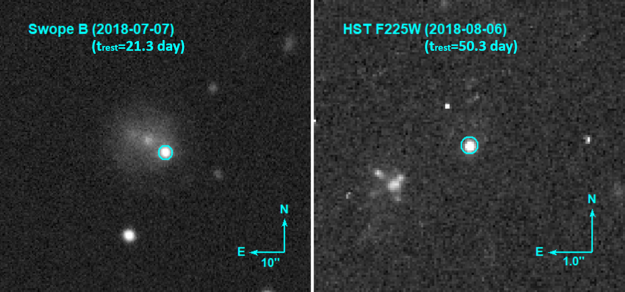
Figure 1: Example cutout images of the field of AT 2018cow taken by Swope (left) and HST (right). The filter and observation date are shown at the top, and a circular aperture is placed at the position of AT 2018cow. The high-resolution HST image shows AT 2018cow as an isolated point source not affected by any significant contamination from the diffuse background or nearby sources.

Table 1: HST photometry of AT 2018cow

Filter	Magnitude (AB)
	$50.3\,\mathrm{d}$	$55.9\,\mathrm{d}$	$60.1\,\mathrm{d}$
F218W	$20.89(0.02)$	$21.29(0.03)$	$21.54(0.04)$
F225W	$20.68(0.01)$	$21.08(0.02)$	$21.30(0.03)$
F275W	$20.37(0.02)$	$20.72(0.02)$	$20.97(0.03)$
F336W	$20.12(0.02)$	$20.69(0.03)$	$20.81(0.03)$

Note. — 1$\sigma$ errors are given inside the brackets.

2 Observations and Data Reduction

In this section, we describe the observations used throughout this study. While our focus is on new constraints that can be derived from late-time HST observations of AT 2018cow, our modeling is supplemented by observations from other facilities/wavelengths. In Figure 1, we show example images of the containing AT 2018cow taken by the 1 m Swope telescope at Las Campanas Obervatory (left) and HST (right) for comparison. In addition to photometric observations described in this section, in Appendix A, we also present a series of previously unpublished spectra, including a high-resolution spectrum taken at $t=4.77\,\mathrm{days}$.

2.1 HST Observations ($t\simeq 50-60\,\mathrm{days}$)

The HST first observed the prompt emission of AT 2018cow (PI Foley) with the Wide Field Camera 3 (WFC3) at three late-time epochs (MJD = 58336.4, 58342.1, 58346.4, or $t\simeq 50.3,\,55.9,\,60.1\,\mathrm{days}$). Observations were obtained in four UVIS bands (F218W, F225W, F275W, F336W) spanning $\lambda\simeq 2224\,\mathrm{\AA}-3355\,\mathrm{\AA}$, designed to track the fading UV emission as it fell below the detection limit of Swift-UVOT. The HST data can be found on the Mikulski Archive for Space Telescopes (MAST): http://dx.doi.org/10.17909/5ry6-7r85 (catalog 10.17909/5ry6-7r85). In the high-resolution HST images, AT 2018cow is seen as an isolated point source without significant background contamination (e.g., Figure 1), allowing precise measurements of its late-time UV flux.

All HST observations were reduced using the hst123 pipeline (Kilpatrick, 2021) as described in Kilpatrick et al. (2022). Each calibrated (flc) WFC3/UVIS frame was downloaded from MAST and aligned to a common reference frame using TweakReg (Hack et al., 2021). We then drizzled each individual epoch and band using drizzlepac before performing point-spread function (PSF) photometry in the original flc frames with dolphot (Dolphin, 2016). We used standard parameters for dolphot as described in the WFC3 guide and hst123 documentation. As a reference frame for dolphot, we used drizzled imaging in WFC3/UVIS F336W obtained at $t\simeq 50.3\,\mathrm{days}$. This image was aligned to all flc frames both in TweakReg and subsequently by alignment methods in dolphot, with the rms uncertainty in frame-to-frame alignment ranging from 0.005–0.049″. Final HST photometry of AT 2018cow are presented in Table 1 and shown in Figure 2 as stars.

We note that Sun et al. (2022) also reported photometry of AT 2018cow from the first three HST observations, but did not analyze these photometry in their study. We find our photometry to generally be consistent with those reported by Sun et al. (2022).

2.2 Swift-UVOT Observations ($t\sim 3-70\,\mathrm{days}$)

To provide context for the UV evolution of AT 2018cow prior to the HST observations, we used data from the Ultra-Violet Optical Telescope (UVOT; Roming et al., 2005) onboard the Neil Gehrels Swift Observatory (Swift; Gehrels et al., 2004). Swift observations of AT 2018cow began from $t\simeq 3\,\mathrm{days}$ and continued for $\sim$70 days (although later epochs suffered from significant background contamination). The UVOT observations covered all six bands ($uw1$, $uw2$, $um2$, $uvu$, $uvb$, $uvv$), spanning the wavelength range of $\lambda_{\mathrm{eff}}\simeq 2086\,\mathrm{\AA}-5411\,\mathrm{\AA}$. Note that $uvu$, $uvb$, and $uvv$ refer to the UVOT $u$, $b$, and $v$ bands.

While Swift-UVOT data of AT 2018cow have previously been published (e.g. Perley et al., 2019; Kuin et al., 2019), in September 2020, a new UVOT sensitivity calibration file was released to account for the loss of sensitivity in the UV and white filters. This retroactively applied to all UVOT observations after 2017, including those of AT 2018cow, with a possible difference up to 0.3 mag. For this reason, we performed our own analysis using an updated UVOT caldb (20201008 release).

We downloaded the reduced level 2 sky images of AT 2018cow from the Swift archive. Images were discarded if AT 2018cow landed on a patch of the detector with reduced sensitivity. Multi-extension images were combined using uvotimsum with default parameters whenever possible. We used uvotsource to perform aperture photometry on AT 2018cow. The source region was chosen to be a 3″ circular aperture, while the background region was chosen to be a 30″ circular aperture in an empty sky region away from the host galaxy. Aperture corrections were applied to the photometry using the curve-of-growth method.

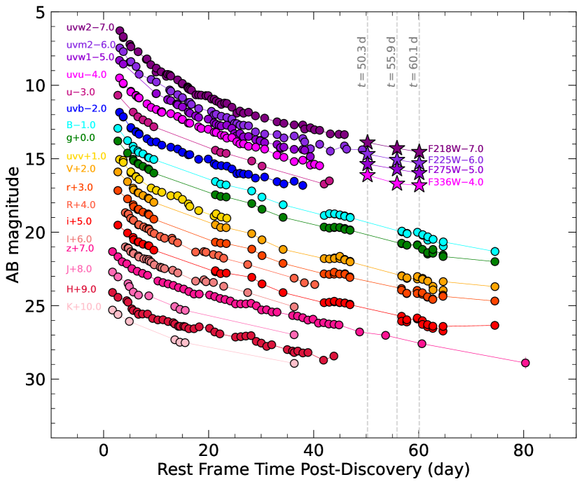
Figure 2: The final multi-band UVOIR light curves of AT 2018cow used in this study. The HST photometry are shown as stars, and the HST epochs are marked with dashed lines. Magnitudes are shifted for visual clarity. UVOT photometry are included only if they are above the $3\sigma$ detection level. The photometry shown is available as Data behind the Figure.

To account for local background contamination, we applied the same source and background apertures to UVOT images of the host galaxy taken in MJD 58761 (or $t\simeq 467\,\mathrm{days}$) and measured the background emission at the location of AT 2018cow. We then subtracted the measured background flux from the fluxes of AT 2018cow obtained in the previous step. Based on this analysis, we found that AT 2018cow was robustly detected ($>3\sigma$) by Swift out to $t\sim 40-50\,\mathrm{days}$.

Compared to previously published Swift-UVOT photometry in studies of AT 2018cow (e.g., Perley et al., 2019; Kuin et al., 2019), our photometry are generally very consistent (within error), with differences much less than 0.3 mag. We note that a more recent paper, Hinkle et al. (2021), used the updated calibration file and published corrected Swift-UVOT photometry of TDE candidates, including AT 2018cow. However, our photometry (and previously published ones) are inconsistent with the photometry in Hinkle et al. (2021), with differences up to $\approx 0.8$ mag. Given that these differences are larger than the expected correction, we chose to use photometry derived from our analysis. The $>3\sigma$ Swift-UVOT photometry used in this study are shown in Figure 2.

2.3 Swope Observations ($t\sim 3-75\,\mathrm{days}$)

To constrain the SEDs of the prompt emission of AT 2018cow, particularly at the time of the HST observations, we required optical data at similar epochs. We obtained photometry from the 1 m Swope Telescope at the Las Campanas Observatory, Chile, which started observing AT 2018cow at $t\sim 3\,\mathrm{days}$ and continued for $\sim$70 days. The observations covered the $uBgVri$ bands, spanning the wavelength range $\lambda_{\mathrm{eff}}\simeq 3608\,\mathrm{\AA}-7458\,\mathrm{\AA}$.

Following the reduction procedures described in Kilpatrick et al. (2018), all image processing and optical photometry on the Swope data was performed using photpipe (Rest et al., 2005), including bias-subtraction, flat-fielding, image stitching, registration, and photometric calibration. The $BgVri$ photometry were calibrated using standard sources from the Pan-STARRS DR1 catalog (Flewelling et al., 2020), and the $u$-band data were calibrated using SkyMapper u-band standards (Onken et al., 2019), both in the same field as AT 2018cow, and transformed into the Swope natural system (Krisciunas et al., 2017) with the Supercal method (Scolnic et al., 2015).

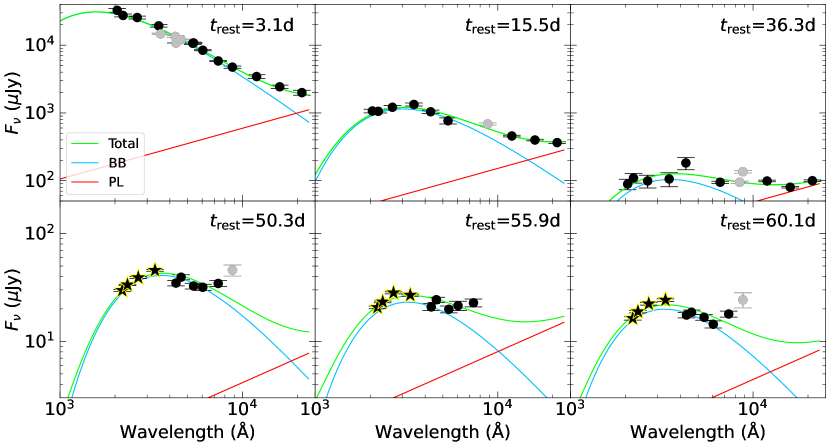
Figure 3: The observed (dereddened) SEDs (black) of AT 2018cow at six sample epochs including the three HST epochs (bottom panels). The HST measurements are marked as stars. The best-fit models (solid lines) are also shown, derived using the blackbody + power law model. Photometry excluded from the fit are shown in gray (see text for reasoning). The UV-optical continuum of AT 2018cow at $t\simeq 50-60\,\mathrm{days}$ is consistent with a blackbody curve peaking at $\lambda\sim 3000\,\mathrm{\AA}$.

To ensure precise measurements at late times, when background contamination from a nearby star-forming region (Figure 1) becomes significant, we obtained deep $uBgVri$ observations between 2019-04-10 and 2021-04-27 with the same telescope and instrument configuration and performed image subtraction using hotpants (Becker, 2015). Forced photometry was performed on the subtracted images to obtain the final photometry shown in Figure 2. We note that our Swope photometry are also generally consistent with previously published photometry in the $uBgVri$ bands from different telescopes (e.g., Perley et al., 2019).

2.4 NIR Photometry ($t\sim 2-80\,\mathrm{days}$)

We also make use of the $RIzJHK$ photometry published by Perley et al. (2019), which span $t\sim 2-80\,\mathrm{days}$. These measurements were taken by the 2 m Liverpool Telescope (Steele et al., 2004), the 1 m telescope at the Mount Laguna Observatory (Smith & Nelson, 1969), the 1.5 m telescope at the Cerro Tololo Inter-American Observatory, the 2 m Himalayan Chandra Telescope, the 0.4 m telescope at Lulin Observatory, the Palomar 200-inch Hale Telescope, and the MPG/ESO 2.2 m telescope (Greiner et al., 2008) at La Silla Observatory. For details on image processing, calibration, and host subtraction, see Section 2.2 of Perley et al. (2019).

3 Evolution of Prompt UVOIR Emission

Our final multi-band UVOIR light curves from the prompt emission ($t\sim 2-80\,\mathrm{days}$) of AT 2018cow are shown in Figure 2. The addition of the HST measurements provides significantly improved constraints on the UV emission beyond the coverage of Swift. In this section, we describe our updated analysis of the prompt UVOIR emission of AT 2018cow, with an emphasis on the later epochs ($t\sim 40-60$ days).

3.1 Constructing UVOIR SEDs

To construct the SEDs, we linearly interpolated the light curves to a common set of epochs. We selected a total of 22 epochs, including the three HST epochs, that have sufficient UV-optical spectral coverage. The errors in the interpolated magnitudes were found through Monte Carlo propagation. At each epoch, we only interpolated a given light curve if the nearest measurement was within 1.0 days from the epoch. The only exception was the first HST epoch ($t=50.3\,\mathrm{days}$) which did not have any measurements in the optical bands within 1.0 days. For this epoch, we interpolated all the optical bands regardless and added 0.03 mag (approximately 3% of flux) to the uncertainties of the interpolated magnitudes to account for deviation from linear interpolation.

3.2 SED Shape at $t\simeq 50-60\,\mathrm{days}$

The precision of the HST photometry allows for the most accurate assessment to date of the UV-optical SED of AT 2018cow at $t\simeq 50-60\,\mathrm{days}$. As shown in the bottom panels of Figure 3, the HST photometry trace a smooth curve peaking at $\lambda\sim 3000\,\mathrm{\AA}$ with an exponential decay in the NUV. The shape of the SEDs at these times resembles a blackbody (Section 3.3), similar to the previous epochs, suggesting optically thick emission even at these late epochs despite the rapid fading. The smooth continuum in the NUV ($\lambda\sim 2000-3000\,\mathrm{\AA}$) also implies a lack of line blanketing from iron peak elements. We highlight the spectral shape here because our results (Section 3.4) and interpretations (Section 4) are heavily influenced by this property.

3.3 Modeling of the UVOIR SEDs

We performed forward modeling to characterize the UVOIR SEDs of AT 2018cow. In summary, we defined a theoretical spectrum to model the emission of the transient, reddened the spectrum according to the Cardelli extinction law (Cardelli et al., 1989) with $R_{\mathrm{V}}=3.1$, and performed synthetic photometry to obtain the model magnitude in each band. Finally, we fit the model SED to the observed SED using the Markov Chain Monte Carlo (MCMC) sampler in the Python package emcee (Foreman-Mackey et al., 2013). The best-fit model parameters and uncertainties were derived from the 50th, 15.9th, and 84.1th percentile of the resulting samples.

Regarding the theoretical spectrum, it is well-established that a blackbody can characterize most of the UV-optical emission of AT 2018cow when the transient was still bright (Perley et al., 2019; Margutti et al., 2019; Kuin et al., 2019). In addition, a second component was found to be necessary at all times to account for excess IR emission. The main objective of this study is to constrain the late thermal properties of AT 2018cow using UV measurements from the HST. Therefore, we followed Perley et al. (2019) and adopted a model in the form of blackbody + power law (BB + PL). The thermal properties are extracted directly through the blackbody while the power law describes the excess IR emission phenomenologically.

In the model blackbody + power law, the blackbody is simply the Planck function $B_{\nu}(T)$, while the power law takes the form $F_{\nu,\mathrm{PL}}\propto\nu^{\alpha}$. Following Perley et al. (2019), the spectral index is fixed at $\alpha=-0.75$ for all epochs. The total flux density from the theoretical spectrum is then given by

$$f_{\nu} = F_{\nu,\mathrm{BB}}(R_{\mathrm{BB}},T_{\mathrm{BB}})+F_{\nu,\mathrm{PL}}(A_{\mathrm{PL}})$$ (1)

$$= \frac{\pi R_{\mathrm{BB}}^{2}}{d_{\mathrm{L}}^{2}}B_{\nu}(T_{\mathrm{BB}})+A_{\mathrm{PL}}\nu^{-0.75}$$

where $d_{\mathrm{L}}$ is the luminosity distance and the three free parameters are the blackbody radius $R_{\mathrm{BB}}$, the blackbody temperature $T_{\mathrm{BB}}$, and the power law constant $A_{\mathrm{PL}}$. At the end of the fitting procedure, we obtain the best-fit $R_{\mathrm{BB}}$, $T_{\mathrm{BB}}$, and $A_{\mathrm{PL}}$.

During fitting, we followed Perley et al. (2019) and removed two clearly visible broad spectral features from the SEDs: the $Bbg$ data before $t=11\,\mathrm{days}$ and the $Iz$ data after $t=10\,\mathrm{days}$. The former is a broad absorption trough centered at approximately 4600 Å while, the latter is a broad emission bump around 9000 Å. We did not attempt to characterize these features in our models.

Figure 3 shows the best-fit models and observed SEDs at six sample epochs, including the three HST epochs. At early epochs, results from our fitting procedure are consistent with previous studies: (i) the UV-optical continuum was very consistent with a blackbody curve, (ii) the power law describes the excess IR emission reasonably well, and (iii) over time, the amplitude of the continuum decreased while the peak shifts from the NUV towards the optical. At the HST epochs, with precise UV photometry, we confirmed that the UV-optical continuum was still consistent with a blackbody curve (see $\chi^{2}/\mathrm{d.o.f}$ in Table 2), i.e., optically thick. Furthermore, the spectral shape remained almost constant at these times, with a peak at $\lambda\sim 3000\,\mathrm{\AA}$.

Based on the best-fit models, we also derived the UVOIR continuum bolometric luminosities of AT 2018cow. The luminosity of the blackbody was taken simply as

$$L_{\mathrm{BB}}=4\pi R_{\mathrm{BB}}^{2}\sigma T_{\mathrm{BB}}^{4}$$ (2)

where $\sigma$ is the Stefan-Boltzmann constant. The luminosity of the power law was calculated through

$$L_{\mathrm{PL}}=4\pi d_{\mathrm{L}}^{2}A_{\mathrm{PL}}\left.\frac{\nu^{\alpha+1}}{\alpha+1}\right|_{\lambda=2\times 10^{3}\,\mathrm{\AA}}^{\lambda=10^{7}\,\mathrm{\AA}}$$ (3)

where $\alpha=-0.75$. Note that the integration range for the power law luminosity is arbitrarily chosen (covering most of the IR range) due to the lack of constraints, so the derived values should be treated with caution.

Finally, we note that it has also been suggested that dust could account for the excess IR emission (e.g., Xiang et al., 2021; Metzger & Perley, 2023). For this case, we checked to see if changing the power law to a dust model would impact the thermal properties derived from the blackbody. We performed fits in Appendix B using a model in the form of blackbody + dust and found that the thermal properties derived from the blackbody are robust and largely unaffected by the description of the excess IR emission.

Table 2: Properties of AT 2018cow derived from the blackbody + power law model

$t\,(\mathrm{day})$	$R_{\mathrm{BB}}\,(R_{\odot})$	$T_{\mathrm{BB}}\,(\mathrm{K})$	$A_{\mathrm{PL}}\,(\mathrm{kJy}\,\mathrm{Hz}^{0.75})$	$L_{\mathrm{BB}}\,(10^{41}\,\mathrm{erg}\,\mathrm{s}^{-1})$	$L_{\mathrm{PL}}\,(10^{41}\,\mathrm{erg}\,\mathrm{s}^{-1})$	$\chi^{2}/\mathrm{d.o.f}$
3.09	$10390.54^{+293.42}_{-292.89}$	$32389.87^{+1200.87}_{-1093.39}$	$42810.74^{+4923.90}_{-4787.35}$	$4098.93^{+380.77}_{-328.24}$	$40.44^{+4.65}_{-4.52}$	7.29
3.75	$9791.83^{+261.03}_{-254.74}$	$30239.58^{+1006.62}_{-945.66}$	$46862.01^{+4272.03}_{-4149.33}$	$2765.90^{+231.50}_{-206.24}$	$44.26^{+4.04}_{-3.92}$	8.46
5.20	$9069.67^{+218.83}_{-215.65}$	$24888.00^{+723.03}_{-691.59}$	$31603.12^{+1608.62}_{-1610.10}$	$1087.97^{+76.51}_{-70.27}$	$29.85^{+1.52}_{-1.52}$	3.24
6.18	$7312.00^{+188.23}_{-188.46}$	$26147.57^{+767.39}_{-742.33}$	$25514.71^{+1836.36}_{-1908.38}$	$861.17^{+60.96}_{-54.51}$	$24.10^{+1.73}_{-1.80}$	6.98
6.57	$7409.44^{+201.46}_{-191.95}$	$24450.06^{+766.24}_{-752.87}$	$21024.99^{+1702.87}_{-1616.00}$	$676.87^{+49.88}_{-47.63}$	$19.86^{+1.61}_{-1.53}$	6.93
8.26	$7398.53^{+205.56}_{-194.68}$	$20860.37^{+550.49}_{-549.81}$	$27343.18^{+1823.33}_{-1851.81}$	$357.51^{+20.06}_{-19.59}$	$25.83^{+1.72}_{-1.75}$	12.72
9.05	$6780.06^{+164.11}_{-161.35}$	$20656.62^{+495.64}_{-452.31}$	$23496.85^{+1396.62}_{-1404.06}$	$288.65^{+14.72}_{-12.66}$	$22.19^{+1.32}_{-1.33}$	13.81
10.04	$6057.73^{+154.69}_{-158.02}$	$21059.10^{+526.03}_{-515.52}$	$18246.62^{+1211.06}_{-1224.30}$	$248.71^{+13.34}_{-12.41}$	$17.24^{+1.14}_{-1.16}$	7.76
13.56	$5801.13^{+177.65}_{-166.56}$	$18053.47^{+387.80}_{-379.63}$	$12662.24^{+539.95}_{-523.22}$	$123.27^{+4.53}_{-4.12}$	$11.96^{+0.51}_{-0.49}$	1.71
14.53	$5471.49^{+188.58}_{-166.53}$	$17694.89^{+392.56}_{-403.78}$	$10691.38^{+462.76}_{-439.73}$	$101.18^{+3.83}_{-3.41}$	$10.10^{+0.44}_{-0.42}$	1.00
15.54	$5344.10^{+232.54}_{-219.13}$	$16818.06^{+446.58}_{-423.34}$	$10933.35^{+514.38}_{-529.27}$	$78.80^{+2.95}_{-2.56}$	$10.33^{+0.49}_{-0.50}$	1.57
21.29	$3542.78^{+108.92}_{-110.16}$	$16072.67^{+396.12}_{-369.71}$	$10824.82^{+544.97}_{-571.80}$	$28.87^{+1.21}_{-1.05}$	$10.22^{+0.51}_{-0.54}$	9.46
22.28	$3381.20^{+129.20}_{-126.69}$	$15719.83^{+428.84}_{-401.72}$	$9542.58^{+729.34}_{-712.72}$	$24.08^{+0.91}_{-0.88}$	$9.01^{+0.69}_{-0.67}$	12.92
23.37	$3014.36^{+154.47}_{-152.37}$	$16331.95^{+574.30}_{-536.04}$	$12688.59^{+964.25}_{-943.23}$	$22.31^{+0.99}_{-0.96}$	$11.99^{+0.91}_{-0.89}$	14.69
28.22	$3055.34^{+139.35}_{-140.42}$	$13575.65^{+423.38}_{-379.05}$	$9216.13^{+514.69}_{-548.52}$	$10.95^{+0.43}_{-0.39}$	$8.71^{+0.49}_{-0.52}$	8.09
30.17	$2338.37^{+139.42}_{-143.08}$	$14631.13^{+654.20}_{-534.25}$	$6019.21^{+492.78}_{-510.99}$	$8.67^{+0.51}_{-0.43}$	$5.69^{+0.47}_{-0.48}$	8.89
34.19	$1404.86^{+132.66}_{-123.36}$	$17659.87^{+1328.23}_{-1159.81}$	$4369.81^{+399.32}_{-373.34}$	$6.62^{+0.85}_{-0.67}$	$4.13^{+0.38}_{-0.35}$	2.34
36.27	$2010.08^{+138.44}_{-135.02}$	$14522.74^{+808.41}_{-724.78}$	$3478.06^{+110.78}_{-110.37}$	$6.20^{+0.67}_{-0.58}$	$3.29^{+0.10}_{-0.10}$	9.89
43.84	$998.05^{+115.05}_{-109.48}$	$18023.01^{+1847.57}_{-1513.66}$	$2533.21^{+243.13}_{-237.60}$	$3.63^{+0.66}_{-0.51}$	$2.39^{+0.23}_{-0.22}$	2.63
50.25	$1314.05^{+47.20}_{-53.26}$	$14121.14^{+200.01}_{-190.78}$	$299.12^{+227.85}_{-186.33}$	$2.37^{+0.07}_{-0.09}$	$0.28^{+0.22}_{-0.18}$	5.27
55.87	$828.62^{+56.45}_{-58.61}$	$15868.78^{+465.19}_{-421.43}$	$579.05^{+204.64}_{-190.43}$	$1.50^{+0.07}_{-0.07}$	$0.55^{+0.19}_{-0.18}$	7.15
60.11	$793.56^{+50.75}_{-51.30}$	$15541.62^{+429.19}_{-388.80}$	$319.48^{+140.67}_{-135.18}$	$1.27^{+0.05}_{-0.05}$	$0.30^{+0.13}_{-0.13}$	7.66

Note. — Errors given here are statistical errors from the 15.9th and 84.1th percentile. The degrees-of-freedom ($d.o.f$) is taken to be the number of data points minus the number of free model parameters.

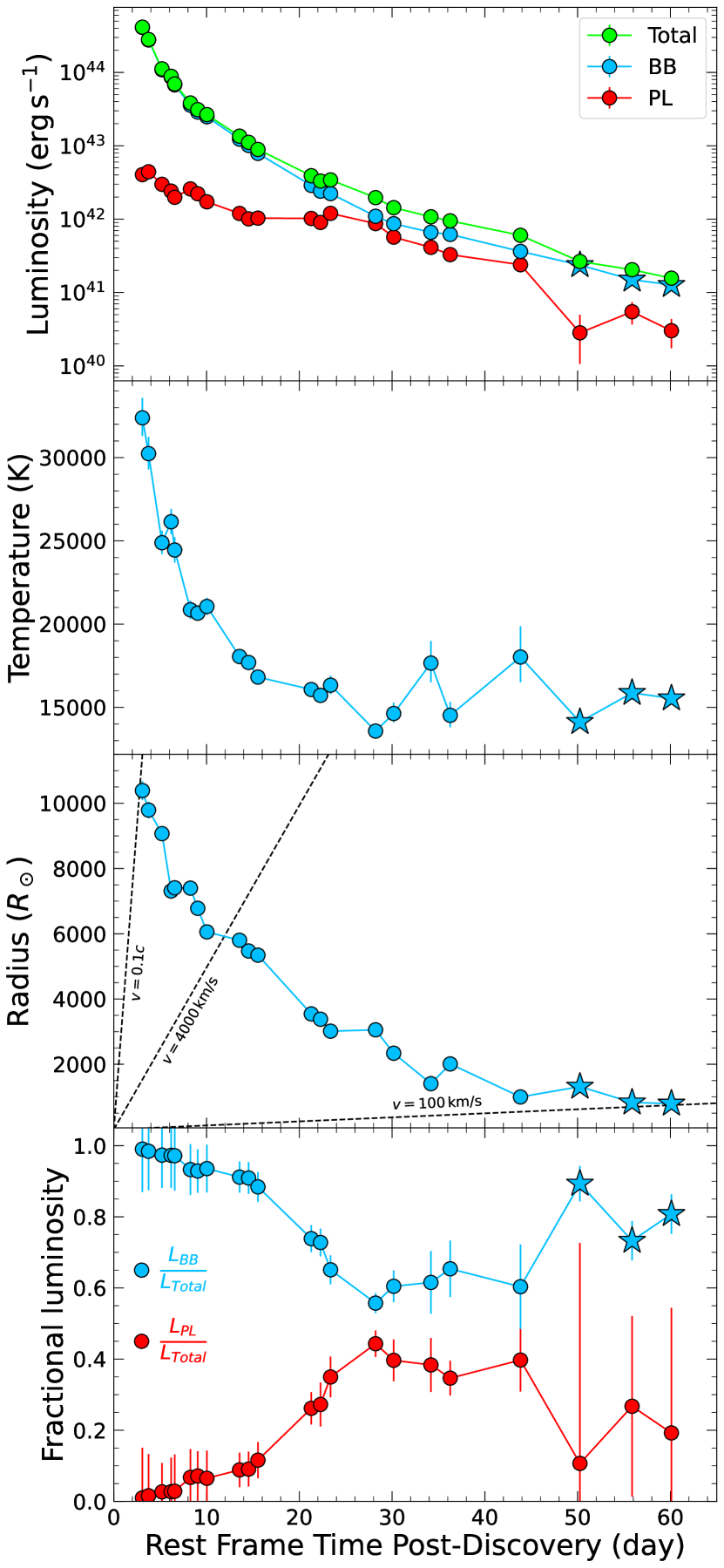
Figure 4: Properties derived from fitting blackbody + power law model. Properties derived using HST photometry are shown as stars. The blackbody luminosity was calculated through the Stefan-Boltzmann law while the power law luminosity was calculated by integrating between $2000\,\mathrm{\AA}\leq\lambda\leq 1\,\mathrm{mm}$.

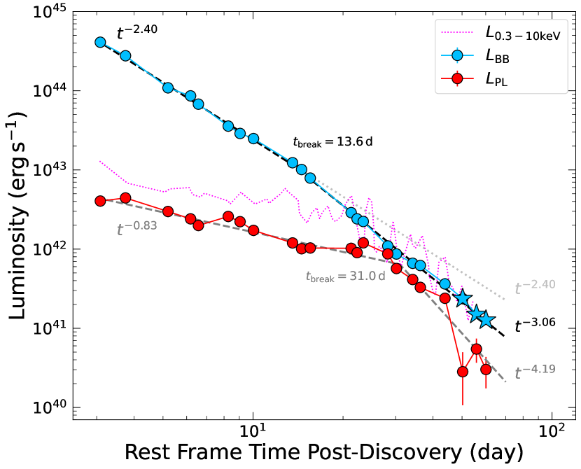
Figure 5: The blackbody luminosity and power law luminosity ($L_{\mathrm{BB}}$ and $L_{\mathrm{PL}}$) derived from the blackbody + power law model, as well as the Swift $0.3-10\,\mathrm{keV}$ luminosity from Margutti et al. (2019) are shown (similar X-ray light curves were also derived in Rivera Sandoval et al. 2018, Kuin et al. 2019, and Ho et al. 2019). Blackbody luminosities derived using HST photometry are shown as stars. Best-fit broken power laws to the luminosities are shown in dashed lines. A dotted line is shown to illustrate the expected decline of the blackbody luminosity if the rate of decline stayed at $t^{-2.40}$.

3.4 Updated Thermal Properties ($t\sim 3-60\,\mathrm{days}$)

The best-fit parameters, derived bolometric luminosities, and the reduced chi-square $\chi^{2}/d.o.f$ from fitting blackbody + power law at all 22 epochs are given in Table 2 and plotted over time in Figure 4.

In general, our results at the earlier epochs are consistent with previous studies (e.g., Perley et al., 2019), namely the high peak luminosity ($L_{\mathrm{BB,peak}}\sim 4\times 10^{44}\,\mathrm{erg}\,\mathrm{s}^{-1}$) and peak temperature ($T_{\mathrm{BB,peak}}\sim 30000\,\mathrm{K}$), the continuously receding blackbody radius, the temperature plateau at $T_{\mathrm{BB}}\sim 15000\,\mathrm{K}$ after $t\sim 15\,\mathrm{days}$, and the increasingly significant IR excess. At the later HST epochs, we found that the temperature remained high at $T_{\mathrm{BB}}\sim 15000\,\mathrm{K}$ while the radius decreased to $R_{\mathrm{BB}}\lesssim 1000\,R_{\odot}$, a size comparable to that of a red supergiant. These late thermal properties derived from the HST photometry are more precise compared to previous studies and suggest that the UV-optical continuum of AT 2018cow at $t\simeq 50-60\,\mathrm{days}$ comes from deeply-embedded hot thermalized material.

We further examined the bolometric light curves and performed simple fits to characterize their decline, shown in Figure 5. With the more precise late thermal properties, we report here a new finding: the luminosities decline faster at later epochs. Our initial attempt to model the decline with a single power law, following previous studies, yielded unsatisfactory fits ($\chi^{2}_{\mathrm{PL}}/d.o.f=12.2$), and we instead found that a broken power law performed much better ($\chi^{2}_{\mathrm{bknPL}}/d.o.f=2.8$). From fitting a broken power law, we found that the blackbody luminosity declined at a rate of $t^{-2.40}$ before $t_{\mathrm{break}}=13.6\,\mathrm{days}$, similar to the expectations of central engine scenarios where $L\propto t^{-\alpha}$ with $\alpha\approx 2-2.5$ (Margutti et al., 2019, and references therein). At $t>13.6\,\mathrm{days}$, the blackbody luminosity started declining at a faster rate of $t^{-3.06}$. The $t_{\mathrm{break}}=13.6\,\mathrm{days}$ is reminiscent of the transition point marked by the emergence of intermediate-width emission lines and the appearance of rapid X-ray variability. The decline in the blackbody luminosity at the later epochs is also very similar to the decline in the soft X-ray luminosity (Figure 5), which may indicate a correlation. We found a similar pattern for the power law luminosity, where the decline was initially gradual ($t^{-0.83}$) but became much faster ($t^{-4.23}$) after $t=31.5\,\mathrm{days}$. However, we note that the power law luminosity is poorly constrained due to the lack of IR data (see Figure 2 and 3) and ambiguity regarding the origin of the excess IR emission.

The updated thermal properties, derived from including the HST photometry, are summarized below.

• At $t\simeq 50-60\,\mathrm{days}$, the NUV-optical spectral shape is fully consistent with a blackbody that has a high temperature ($T_{\mathrm{BB}}\sim 15000\,\mathrm{K}$) and a small radius ($R_{\mathrm{BB}}\lesssim 1000\,R_{\odot}$).

• The blackbody luminosity is better characterized by a broken power law that declined at a rate of $t^{-2.40}$ before a break at $t_{\mathrm{break}}=13.6\,\mathrm{days}$, and declined much faster at $t^{-3.06}$ after the break.

The combination of optically thick emission, high temperature, and rapid decline in blackbody luminosity at $t\simeq 50-60\,\mathrm{days}$ is a unique feature of AT 2018cow, even in the context of FBOTs, which we discuss in more detail in Section 4.

4 Constraints on the Power Source of the Fading Prompt Emission ($t\sim 20-60\,\mathrm{days}$)

Through our analysis of the HST photometry, we showed that the UV-optical emission of AT 2018cow at $t\simeq 50-60\,\mathrm{days}$ was very consistent with a blackbody that has a high temperature ($T_{\mathrm{BB}}\sim 15000\,\mathrm{K}$) and a small radius ($R_{\mathrm{BB}}\sim 1000\,R_{\odot}$). The natural interpretation of these results, given the lack of an observed nebular phase, is that the emission was still optically thick after two months and originated from thermalized material in the deeper regions. These thermal properties imply that there existed a power source (or multiple) that was still injecting energy at the later epochs. With the improved constraints, we also discovered that the blackbody luminosity declined faster after $t\sim 15\,\mathrm{days}$, at a rate of $L_{\mathrm{BB}}\propto t^{-3.06}$, possibly associated with the evolution of the power source.

In this section, we discuss the implications of our findings and place constraints on possible power sources of the fading prompt emission ($t\sim 20-60\,\mathrm{days}$) of AT 2018cow through comparisons with the literature and simple model estimates. We focus on three specific power sources generally favored by previous studies: radioactive decay (Section 4.1), ejecta-CSM interaction (Section 4.2), and central engine activity (Section 4.3).

4.1 Radioactive Decay

Generally, radioactive decay has been disregarded as the dominant power source of AT 2018cow because an unphysical amount of ⁵⁶Ni ($>5\,M_{\odot}$) would be required to produce the peak luminosity (Margutti et al., 2019; Perley et al., 2019). Still, the possible existence of a small amount of ⁵⁶Ni has not been ruled out, which could have partially contributed to the observed thermal emission, especially at the later epochs. Constraining the mass of the ⁵⁶Ni may also help distinguish possible progenitor systems and whether or not fallback is necessary to explain the lack of ⁵⁶Ni.

Studies such as Xiang et al. (2021) and Pellegrino et al. (2022) have modeled previously published bolometric light curve of AT 2018cow using a combination of ejecta-CSM interaction and radioactive decay and argued that radioactive decay could fully account for the emission after $t\sim 25\,\mathrm{days}$. They inferred a ⁵⁶Ni mass of $M_{\mathrm{Ni}}\sim 0.1-0.3\,M_{\odot}$ from their models.

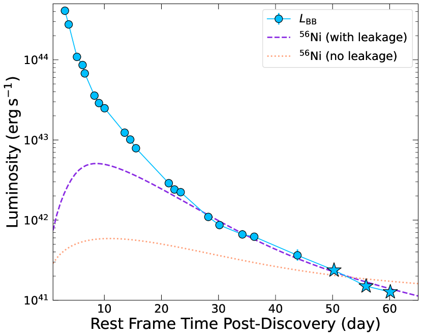
Figure 6: The blackbody luminosity of AT 2018cow ($L_{\mathrm{BB}}$) and the best-fit radioactive decay models (⁵⁶Ni) for the light curve after 25 days. The model without $\gamma$-ray leakage cannot fit the light curve at all while the model with $\gamma$-ray leakage can fully describe the light curve after $t\sim 25\,\mathrm{days}$.

We also modeled our updated bolometric light curve to investigate whether radioactive decay can power the late thermal emission and be consistent with the faster fading ($L_{\mathrm{BB}}\propto t^{-3.06}$) discovered in this study. Specifically, we used the semi-analytical model for radioactive decay from Chatzopoulos et al. (2012) that includes radiation diffusion to fit the thermal bolometric light curve at $t>25\,\mathrm{days}$. We considered two cases, one including $\gamma$-ray leakage through the factor $(1-e^{-(t/T_{0})^{-2}})$, where $T_{0}$ is the trapping timescale, and the other assuming no leakage ($T_{0}\rightarrow\infty$). For both cases, we adopted an optical opacity of $\kappa_{\mathrm{opt}}=0.2\,\mathrm{cm}^{2}\,\mathrm{g}^{-1}$.

Figure 6 shows the best-fit models and Table 3 gives the best-fit parameters. Without leakage, radioactive decay cannot reproduce the late-time light curve shape and even a small mass of $M_{\mathrm{Ni}}=0.019\,M_{\odot}$ overestimates the emission after $t\sim 55\,\mathrm{days}$. For the no-leakage case, we also found an upper limit of $M_{\mathrm{Ni}}\lesssim 0.013-0.019\,M_{\odot}$, which could power the exact luminosity at $t\simeq 60\,\mathrm{days}$ assuming a range of $M_{\mathrm{ej}}=0.1-10\,M_{\odot}$ and $v_{\mathrm{ej}}=0.01c-0.1c$. On the other hand, when leakage is included, radioactive decay models can reproduce both the luminosity and observed decline at $t>25\,\mathrm{days}$ with a $M_{\mathrm{Ni}}=0.675^{+0.490}_{-0.335}\,M_{\odot}$ and a $T_{0}=9.54^{+3.90}_{-2.34}\,\mathrm{days}$.

Although the fit is reasonable when leakage is included, the inferred model parameters are inconsistent with other properties of AT 2018cow. Note that our best-fit ⁵⁶Ni mass is a few times larger than those inferred by Xiang et al. (2021) and Pellegrino et al. (2022). This difference is likely due to the faster decline in our light curve at the later epochs: a faster decline can be produced by a larger $\gamma$-ray leakage (smaller trapping timescale), but a larger leakage reduces the heating and therefore requires a larger ⁵⁶Ni mass. A ⁵⁶Ni mass of $M_{\mathrm{Ni}}\sim 0.3-1.1\,M_{\odot}$ is fairly difficult to explain given the lack of UV blanketing from iron peak elements in AT 2018cow (Margutti et al., 2019). This is especially true considering that both the small trapping timescale and high inferred velocity ($\sim$0.1c; higher than those observed in emission lines at similar epochs) required in this best-fit model could suggest that some fraction of the radioactive material is located in the outer portions of the ejecta. These inconsistencies imply that radioactive decay was unlikely the dominant power source over the entire $t\simeq 25-60\,\mathrm{days}$ period.

Note that if radioactive decay is not required to start dominating at $t\simeq 25\,\mathrm{days}$ but at a later date, then the required $M_{\mathrm{Ni}}$ can be smaller (e.g., $M_{\mathrm{Ni}}\lesssim 0.013-0.019\,M_{\odot}$ would dominate at $t\gtrsim 60\,\mathrm{days}$ assuming no leakage, as discussed above). Although small amounts of Nickel have been observed some SNe Ib/c with small ejecta masses, in most cases, line-blanketing is still observed. For example, in SN 2011hs and SN 2007Y ($\sim$0.02–0.03 M_⊙; Prentice et al. 2016) blanketing due to iron-peak elements suppressed the continuum at $\lambda<5000$ Å to a level below that at longer wavelengths by $\sim$30–40 days post-discovery. Similar behavior was not detected for AT 2018cow. Therefore, based on the constraints set by the lack of UV blanketing, we disfavor radioactive decay as a significant power source for the fading prompt emission of AT 2018cow over $t\simeq 25-60\,\mathrm{days}$, and we argue that alternative power sources are more likely.

4.2 Ejecta-CSM Interaction

The bright radio synchrotron emission from AT 2018cow has clearly revealed the existence of CSM around the progenitor (Margutti et al., 2019; Ho et al., 2019; Nayana & Chandra, 2021). Through radio observations, assuming a density distribution of $\rho=\dot{M}/(4\pi R^{2}v_{\mathrm{w}})$ with $v_{\mathrm{w}}=1000\,\mathrm{km}\,\mathrm{s}^{-1}$, Ho et al. (2019) inferred an $\dot{M}\approx 4\times 10^{-4}\,M_{\odot}\,\mathrm{yr}^{-1}$ within a radius of $R\lesssim 1.7\times 10^{16}\,\mathrm{cm}$ and Nayana & Chandra (2021) inferred an $\dot{M}\lesssim 4\times 10^{-6}\,M_{\odot}\,\mathrm{yr}^{-1}$ at $R\gtrsim 6\times 10^{16}\,\mathrm{cm}$. The decline of $\dot{M}$ over distance suggests more enhanced mass loss closer to the explosion.

Several optical signatures, such as the featureless blue continuum, the narrow and intermediate-width lines, and the asymmetric line profiles, have also been used to argue the possibility that the thermal emission of AT 2018cow was powered by ejecta-CSM interaction (Fox & Smith, 2019; Xiang et al., 2021; Pellegrino et al., 2022). This scenario is quite plausible since a number of studies, through analytical and numerical treatments, have demonstrated that ejecta-CSM interaction can lead to bright rapidly-evolving SNe (e.g., McDowell et al., 2018; Suzuki et al., 2019, 2020; Pellegrino et al., 2022; Maeda & Moriya, 2022; Khatami & Kasen, 2023). Additionally, Fox & Smith (2019) argued in favor of this scenario after finding similarities between AT 2018cow and interacting SNe Ibn and IIn in their light curves and spectra. Following these arguments, studies such as Xiang et al. (2021) and Pellegrino et al. (2022) constructed models to show that ejecta-CSM interaction can power the optical peak of AT 2018cow (and the subsequent emission up to $t\sim 20\,\mathrm{days}$) through a dense shell of CSM with $\dot{M}\sim 1\,M_{\odot}\,\mathrm{yr}^{-1}$ and an outer edge at $R_{\mathrm{out}}\sim 1.0\times 10^{14}\,\mathrm{cm}$. Note that the hypothetical CSM powering the optical peak is orders of magnitude denser than the CSM powering the radio synchrotron emission, which would suggest extreme eruption just before the explosion. Recently, Maund et al. (2023) reported flashes of optical polarization from AT 2018cow at $t\sim 5\,\mathrm{days}$ and $12\,\mathrm{days}$, hinting at an asymmetric configuration and possibly the existence of such dense CSM.

Table 3: Best-fit Radioactive Decay Models

Parameters	With Leakage	No Leakage
$M_{\mathrm{Ni}}$ ($M_{\odot}$)	$0.675^{+0.490}_{-0.335}$	$0.0192^{+0.0005}_{-0.0005}$
$v_{\mathrm{ej}}$ ($\mathrm{km}\,\mathrm{s}^{-1}$)	$5.37^{+7.12}_{-3.94}\times 10^{4}$	$1.71^{+0.91}_{-0.75}\times 10^{3}$
$M_{\mathrm{ej}}$ ($M_{\odot}$)	$5.34^{+3.27}_{-3.63}$	$0.833^{+0.197}_{-0.262}$
$R_{0}$ ($\mathrm{cm}$)	$7.79^{+3.85}_{-4.04}\times 10^{14}$	$11.04^{+2.14}_{-3.46}\times 10^{14}$
$t_{0}$ ($\mathrm{days}$)	$-0.728^{+0.826}_{-0.793}$	$-1.89^{+0.17}_{-0.08}$
$T_{0}$ ($\mathrm{days}$)	$9.54^{+3.90}_{-2.34}$	$\infty$

Note. — $M_{\mathrm{Ni}}$: ⁵⁶Ni mass; $v_{\mathrm{ej}}$: ejecta velocity; $M_{\mathrm{ej}}$: ejecta mass; $R_{0}$: initial radius; $t_{0}$: initial time with respect to MJD 58285.441; $T_{0}$: $\gamma$-ray trapping timescale. Lower and upper errors are from the 15.9th and 84.1th percentile, respectively.

Here, we do not construct another ejecta-CSM interaction model to describe our updated thermal properties. Instead, we discuss the implications of the observational properties through comparisons with existing studies of ejecta-CSM interaction. In particular, we discuss two points below: (1) it is unclear if current ejecta-CSM interaction models for AT 2018cow can sufficiently explain the fading prompt emission at $t\gtrsim 20\,\mathrm{days}$, and (2) the peculiar thermal properties of AT 2018cow are not naturally produced in general studies of aspherical ejecta-CSM interaction.

4.2.1 Current Interaction Models for AT 2018cow

For AT 2018cow, a great advantage of invoking CSM is that an aspherical configuration can qualitatively explain many of the peculiar observational properties. Often, studies will adopt a schematic that involves dense equatorial CSM (e.g., a disk) that leads to free-expanding fast ($v\sim 0.1c$) ejecta near the polar region and slow-moving ($v\lesssim 6000\,\mathrm{km}\,\mathrm{s}^{-1}$) ejecta-CSM interaction near the equator (e.g., Figure 12 in Margutti et al., 2019). At an inclined line of sight, the initial peak of AT 2018cow comes from the fast polar ejecta, and as this ejecta becomes optically thin, the photosphere recedes and reveals the embedded ejecta-CSM interaction along with intermediate-width emission lines at $t\sim 15-20\,\mathrm{days}$. In this scenario, the embedded interaction powers the fading prompt emission over $t\sim 20-60\,\mathrm{days}$ and maintains a temperature plateau at $T_{\mathrm{BB}}\sim 15000\,\mathrm{K}$.

Although this schematic appears excellent qualitatively, a detailed ejecta-CSM interaction model that can reproduce the fading prompt emission of AT 2018cow does not yet exist. In particular, it is unclear whether this scenario can really give rise to the combination of receding photosphere, optically thick emission, and rapid fading discovered in this study ($L\propto t^{-3}$ that persisted for more than a month after the emergence of the intermediate-width emission lines often associated with the embedded interaction). Many uncertainties remain, e.g., the discrepancy between $v\sim 100\,\mathrm{km}\,\mathrm{s}^{-1}$ inferred from $R_{\mathrm{BB}}\sim 1000\,R_{\odot}$ at $t\simeq 60\,\mathrm{days}$ (Figure 4) and $v\sim 3000-6000\,\mathrm{km}\,\mathrm{s}^{-1}$ inferred from the emission lines, and the observed rapid fading versus an expected slow fading due to high optical depth suppressing radiation.

Current studies such as Xiang et al. (2021) and Pellegrino et al. (2022) have only modeled the optical peak of AT 2018cow through spherical ejecta-CSM interaction and their choice of radioactive decay for the emission at $t\gtrsim 25\,\mathrm{days}$ cannot explain the observed late thermal properties. Recently, Khatami & Kasen (2023) presented a general interaction framework involving a single spherical shell of CSM and was able to produce a rapid decline for AT 2018cow in the edge breakout regime (see Figure 14 in Khatami & Kasen, 2023) with a relatively low ejecta mass ($M_{\mathrm{ej}}\sim 0.5\,M_{\odot}$) and supernova energy ($E_{\mathrm{sn}}\sim 0.2\times 10^{51}\,\mathrm{erg}\,\mathrm{s}^{-1}$). However, their current framework does not include spectral or photospheric evolution, and it is also not clear if the shock cooling phase under spherical symmetry can produce the peculiar thermal properties and optically thick emission of AT 2018cow.

Lastly, we note that studies such as Metzger (2022) and Lyutikov (2022) have constructed more complex models for AT 2018cow involving ejecta/wind-CSM interaction and a central engine. The interactions in these models are most likely aspherical, but similar uncertainties are present. In the model by Lyutikov (2022), the apparent receding photosphere was due to the material becoming optically thin over the first month, which is inconsistent with the observed optically thick emission at the end of the second month. The model by Metzger (2022) does not explicitly track the receding photosphere. Therefore, it is unclear if the interaction in these specific models can result in the persistent receding photosphere and optically thick emission, and we instead turn to general simulations for more insights in Section 4.2.2 below.

4.2.2 Other Aspherical Ejecta-CSM Interactions

Since there is a lack of detailed aspherical ejecta-CSM interaction models in the context of AT 2018cow, we turn to more general simulations involving aspherical CSMs for further insights into the observational properties. Note that these simulations typically examine transients with a timescale of $\sim$100s of days, and therefore our brief discussion here will be qualitative.

Suzuki et al. (2019) performed 2-D simulations involving disk CSMs with various masses and viewing angles and derived properties such as the color temperature and blackbody radius, allowing us to make some qualitative comparisons. In their simulations, the color temperature remained high for a long time, but most cases showed an increasing blackbody radius at all times. The only cases with an initial decline in blackbody radius were cases with an edge-on viewing angle, which had significantly prolonged light curves (slow rise and decline). The receding photosphere happens when the ejecta becomes transparent and reveals the disk, after which an expanding photosphere can be seen. These behaviors also demonstrate the effects of radiation diffusion: a large optical depth produces optically thick emission but suppresses the emission and prolongs the light curve. Therefore, general cases of disk interaction do not seem to easily produce the peculiar thermal properties of AT 2018cow, namely the combination of optically thick emission, receding photosphere, and rapidly-declining brightness at the late epochs.

Kurfürst et al. (2020) performed 2-D simulations involving three CSM distributions: an equatorial disk, colliding wind shells, and a bipolar nebula. They derived two properties from their simulations that were also observed for AT 2018cow: the emission line profiles and optical polarization degrees. Interestingly, they found that only interactions with colliding wind shells produced asymmetric emission lines. They also found an optical polarization degree of $\sim 1-2\%$ for cases involving disk and bipolar CSM and $\sim 0.01-0.5\%$ for cases involving colliding wind shells. In the case of AT 2018cow, clear asymmetric lines and an optical polarization degree of $\sim 0.3-2\%$ (Smith et al., 2018; Maund et al., 2023) were observed besides the two high polarization flashes. This comparison suggests complex CSM distributions may need to be considered.

In conclusion, AT 2018cow presents a unique opportunity to study ejecta-CSM interaction but there are still many open questions that are not answered with general simulations. Future detailed studies involving complex CSM distributions will be necessary to determine if ejecta-CSM interaction are capable of producing the combination of receding photosphere, optically thick emission, and rapidly declining luminosity. If ejecta-CSM interaction cannot offer satisfactory (quantitative) explanations for the fading prompt emission of AT 2018cow at $t\sim 20-60\,\mathrm{days}$, it could be an indication that a different power source (e.g., a central engine) dominated at this time.

4.3 Central Engine – Wind-Reprocessed Framework

Central engines (NSs and BHs) are alternative power sources often invoked to explain FBOTs because they can release an enormous amount of energy over a short timescale (e.g., Yu et al., 2015; Kashiyama & Quataert, 2015). Central engines are particularly favored for the case of AT 2018cow because they can also naturally explain the high ejecta energy, low ejecta mass, and persistent X-ray emission (Margutti et al., 2019; Ho et al., 2019). Currently, a variety of central engine scenarios have been proposed to explain AT 2018cow, typically involving jets (Soker et al., 2019; Gottlieb et al., 2022; Soker, 2022) or winds driven by the engine (Yu et al., 2019; Lyutikov & Toonen, 2019; Piro & Lu, 2020; Uno & Maeda, 2020; Lyutikov, 2022; Metzger, 2022) that may interact with pre-existing CSM. Specific scenarios involving TDEs with an IMBH (with $M_{\mathrm{BH}}\lesssim 10^{5}\,M_{\odot}$; see review by Greene et al., 2020) or a SMBH (with $M_{\mathrm{BH}}\gtrsim 10^{5}-10^{6}\,M_{\odot}$) have also been proposed (Perley et al., 2019; Kuin et al., 2019). The proposed scenarios also involve different progenitor systems, such as single or double WD systems producing NSs (Yu et al., 2019; Lyutikov & Toonen, 2019; Lyutikov, 2022) or common envelope evolution involving the engine (Soker et al., 2019; Metzger, 2022; Soker, 2022). Moving forth, to understand the nature of AT 2018cow and similar transients, it is crucial to distinguish different scenarios.

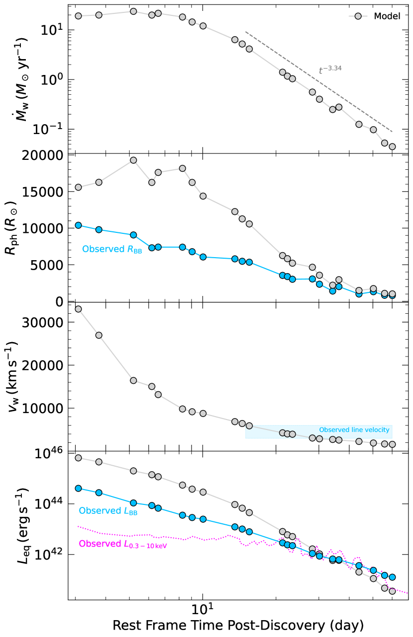
Figure 7: The wind mass-loss rate $\dot{M}_{\mathrm{w}}$ (top panel), photosphere radius $R_{\mathrm{ph}}$ (second panel), wind velocity $v_{\mathrm{w}}$ (third panel), and luminosity at equipartition radius $L_{\mathrm{eq}}$ (bottom panel) derived using observed properties of AT 2018cow based on the wind-reprocessed transient model from Uno & Maeda (2020). A power law fit to the wind mass-loss rate after $t\sim 15\,\mathrm{days}$ is also shown on the top panel. A shaded region is shown on the third panel to indicate the observed emission line velocity $3000\,\mathrm{km}\,\mathrm{s}^{-1}\lesssim v\lesssim 6000\,\mathrm{km}\,\mathrm{s}^{-1}$. Observed properties are also plotted for comparisons with $R_{\mathrm{ph}}$ and $L_{\mathrm{eq}}$.

Often, models will use the rise time and peak optical luminosity to constrain the configurations of the engines. For AT 2018cow, the late thermal properties can also provide additional constraints if the fading prompt emission was associated with a central engine. In particular, the receding photosphere and optically thick emission have significant implications on the evolution of the optical depth and cannot be explained by a simple spherically-expanding engine-powered ejecta. The scenario mostly likely require reprocessing involving some form of wind driven by the engine. Specific configurations of the wind may be able to explain the large optical depth, receding photosphere, and appearance of asymmetric intermediate-width lines. The observed rate of decline in blackbody luminosity at the later epochs ($t^{-3}$) may also constrain the input power of the engine.

Here, we consider an example case and show that a scenario involving wind driven by a central engine can reasonably explain the late thermal properties of AT 2018cow presented in this study. Specifically, we characterize AT 2018cow under the wind-reprocessed framework constructed by Piro & Lu (2020) and Uno & Maeda (2020) (see also Calderón et al., 2021, for numerical simulation). This framework involves continuous outflow/wind driven by a central engine and, following the formulation of Uno & Maeda (2020), relates the observed luminosity and temperature with wind mass-loss rate $\dot{M}_{\mathrm{w}}$, wind (launch) velocity $v_{\mathrm{w}}$, and photosphere radius $R_{\mathrm{ph}}$. Both Piro & Lu (2020) and Uno & Maeda (2020) have modeled AT 2018cow but using previously derived thermal properties (e.g., from Perley et al., 2019). We repeat this modeling to see if our updated properties introduce different interpretations.

Figure 7 shows the model properties derived for AT 2018cow using the formulation from Uno & Maeda (2020). Note that we ignore possible interactions with pre-existing CSM because of the uncertainties discussed in Section 4.2, and also because we are interested in seeing if wind can account for the late-time observational properties without interaction with CSM. Also, since our focus is on the late properties, we will not comment on the performance of the model before $t\sim 15\,\mathrm{days}$. This early emission may or may not be powered by the same mechanism.

The model wind velocity declines steadily after $t\sim 15\,\mathrm{days}$ and is broadly consistent with the velocity derived from the intermediate-width lines that appeared after $t\sim 15\,\mathrm{days}$ ($3000\,\mathrm{km}\,\mathrm{s}^{-1}\lesssim v\lesssim 6000\,\mathrm{km}\,\mathrm{s}^{-1}$). The model photosphere radius also shows a steady decline after $t\sim 15\,\mathrm{days}$, consistent with the observed receding photosphere. We note that although the photosphere and blackbody radii are similar at these epochs, the two are not necessarily comparable because the model photosphere radius takes electron scattering into account. The wind mass-loss rate declines as a power law after $t\sim 15\,\mathrm{days}$ at a rate of $\dot{M}_{\mathrm{w}}\propto t^{-3.35}$. Note that this decline rate is much faster compared to the approximate rate found by Uno & Maeda (2020) and Piro & Lu (2020), $\dot{M}_{\mathrm{w}}\propto t^{-5/3}$, which was consistent with the expected accretion rate for a fallback scenario. The faster decline rate in $\dot{M}_{\mathrm{w}}$ is likely due to the faster decline rate in the blackbody luminosity found in this study. Lastly, we also calculated the luminosity $L_{\mathrm{eq}}$ at the innermost equipartition radius (below which the internal and kinetic energy are in equipartition), which can be interpreted as the engine power. This luminosity is therefore given by $L_{\mathrm{eq}}=\dot{M}_{\mathrm{w}}v_{\mathrm{w}}^{2}/2$. As suggested by Piro & Lu (2020), the similarity between the engine power and the observed X-ray emission at the later epochs is consistent with the reprocessing picture.

Overall, the wind-reprocessed framework can reasonably produce the peculiar thermal properties associated with the fading prompt emission of AT 2018cow. Even the asymmetric line profiles, as suggested by Uno & Maeda (2020), can be explained by an asymmetric distribution of wind outflow. These results could suggest that wind driven by a central engine is sufficient, and ejecta-CSM interaction may not be necessary to account for the fading emission. Lastly, we note that our faster rate of $\dot{M}_{\mathrm{w}}\propto t^{-3.35}$ could have implications on the power output of the engine and the structure of the wind. For example, spherical wind outflow is assumed in these models, which may not be realistic. The actual scenario may have involved wind that was aspherical and outflow that decreased in size over time (i.e., smaller solid angle and lower brightness), which the model would have accounted for by decreasing the wind mass-loss rate.

5 Summary & Conclusion

In this study, we analyzed the first three HST observations of AT 2018cow ($t\simeq 50.3,\,55.9,\,60.1\,\mathrm{days}$) to constrain the late thermal properties of the fading prompt emission. With significantly improved precision in the UV photometry, we confirmed that the fading prompt emission at $t\simeq 50-60\,\mathrm{days}$ is blackbody (i.e., optically thick) with a high temperature ($T_{\mathrm{BB}}\sim 15000\,\mathrm{K}$) and a small radius ($R_{\mathrm{BB}}\lesssim 1000\,R_{\odot}$). Furthermore, we found that although the blackbody luminosity initially declined at a rate of $t^{-2.40}$ (similar with previous findings, e.g., Margutti et al., 2019; Perley et al., 2019), the decline became much faster after $t_{\mathrm{break}}=13.6\,\mathrm{days}$, at a rate of $t^{-3.06}$. The combination of receding photosphere, high temperature, and optically thick emission with a rapidly declining luminosity is very peculiar and places significant constraints on possible power sources for the fading prompt emission.

We disfavor radioactive decay as the dominant power source over $t\simeq 25-60\,\mathrm{days}$ because significant $\gamma$-ray leakage is likely needed to produce the faster decline in luminosity, which drives up the required ⁵⁶Ni mass to $M_{\mathrm{Ni}}\gtrsim 0.3\,M_{\odot}$, inconsistent with the lack of UV line blanketing. Even assuming a $M_{\mathrm{Ni}}\sim 0.01-0.02\,M_{\odot}$, which would be sufficient to start dominating at around $t\sim 50-60\,\mathrm{days}$, the complete lack of blanketing in the HST SEDs is still quite difficult to explain given that the material is already partially optically thin as indicated by the receding photosphere. Therefore, the thermal emission observed at these later epochs is likely powered by an alternative power source.

Although we do not rule out ejecta-CSM interaction as a major contributor to the fading prompt emission, we argue that current models by Xiang et al. (2021) and Pellegrino et al. (2022) are not sufficient in explaining the late thermal properties because of the assumption of spherical symmetry and the dependence on radioactive decay at $t\gtrsim 25\,\mathrm{days}$. Similarly, although the shock cooling phase in the interaction model by Khatami & Kasen (2023) can match the rapid fading of AT 2018cow, it is also not clear if this scenario can explain the spectral and photospheric evolution. Qualitative comparisons with general simulations involving aspherical CSMs (Suzuki et al., 2019; Kurfürst et al., 2020) show that the peculiar thermal properties of AT 2018cow are not easily produced, namely the combination of receding photosphere, optically thick emission, and rapidly declining luminosity. The effects of optical depth in an expanding shock seems to create a major dilemma: material becoming fully optically thin can produce a receding photosphere and rapidly declining luminosity but cannot explain the optically thick emission, while optically thick material would significantly suppress the emission and prolong the light curve. Therefore, whether or not ejecta-CSM interaction can fully explain the late thermal emission of AT 2018cow, and the exact CSM configuration required to do so remain open questions.

On the other hand, we found that the wind-reprocessed framework (Piro & Lu, 2020; Uno & Maeda, 2020) involving continuous outflow/wind driven by a central engine can reasonably explain the late thermal properties of AT 2018cow. In this scenario, the photosphere is receding as earlier winds become optically thin, while the decline in luminosity can be associated with the decline in wind mass-loss rate $\dot{M}_{\mathrm{w}}$ and wind velocity $v_{\mathrm{w}}$ (following the model in Uno & Maeda 2020). Further supporting this scenario, we found the model $v_{\mathrm{w}}$ at $t\gtrsim 20\,\mathrm{days}$ to broadly match the inferred velocity from the intermediate-width lines $v\sim 3000-6000\,\mathrm{km}\,\mathrm{s}^{-1}$. Finally, we found $\dot{M}_{\mathrm{w}}\propto t^{-3.34}$, which is significantly faster than the predicted fallback rate of $\dot{M}\propto t^{-5/3}$, perhaps implying deviation from standard fallback or asymmetric outflow. Overall, these findings suggest that a central engine, without the need to invoke ejecta-CSM interaction, may be sufficient in explaining the fading thermal emission of AT 2018cow.

While the exact progenitor, explosion mechanism, and power source(s) of AT 2018cow are still open to debate, constraints from the late-time HST measurements seem to be pointing towards an accreting central engine. Although an accreting central engine and the wind-reprocessed framework is not needed to explain most extragalactic transients, in the case of AT 2018cow, the unique combination of bright X-ray emission, mildly-relativistic outflow, and persistent optically thick thermal emission can be more consistently explained by the central engine scenario. The continuously receding photosphere (typically not observed in most transients) further associates the observed late-time emission with central activities and itself is much easier to explain with continuous wind/outflow (implying continuous energy injection) rather than a single expanding shock. If this association is true, AT 2018cow and other luminous FBOTs may form an entirely new class of transients powered predominantly by accretion that generates mildly relativistic outflow which powers the initial peak and continuous winds which power the optically thick fading emission. These transients, given the extreme accretion required, would likely involve BHs – either newborn BHs from stellar collapse or (hypothetical) existing IMBH – and bridge the gap between ultra-relativistic transients (e.g., Gamma-Ray Bursts) and non-relativistic transients (e.g., normal SNe). Future observations and additional theoretical works are necessary to confirm or rule out this hypothesis.

Our work also demonstrates the importance of late-time observations in providing additional constraints for unsettled cases such as AT 2018cow. In the fortunate event that another “Cow-like transient” is discovered nearby similar to AT 2018cow, late-time monitoring by HST and JWST can be highly beneficial in differentiating theoretical models and resolving the mysteries of these peculiar transients.

Appendix A Additional Optical Spectroscopy

Here we present a set of previously unpublished optical spectra of AT 2018cow, obtained with the Kast dual-beam spectrograph (Miller & Stone, 1993) on the Lick Shane 3 m telescope, the Levy (Vogt et al., 2014) spectrograph on the 2.4 m Automated Planet Finder (APF) telescope and the Low-Resolution Imaging Spectrograph (LRIS; Oke et al., 1995) on the 10 m Keck I telescope. In each epoch, we aligned the slit to the parallactic angle to minimize the effects of atmospheric dispersion (Filippenko, 1982). A log of all spectroscopic observations is presented in Table 4.

The Kast and LRIS data were reduced using a custom data reduction pipeline (Siebert et al., 2019). The two-dimensional spectra were bias-corrected, flat-field corrected, adjusted for varying gains across different chips and amplifiers, and trimmed. Cosmic-ray rejection was applied using the pzapspec algorithm to individual frames. Multiple frames were then combined with appropriate masking. One-dimensional spectra were extracted using the optimal algorithm (Horne, 1986). The spectra were wavelength-calibrated using internal comparison-lamp spectra with linear shifts applied by cross-correlating the observed night-sky lines in each spectrum to a master night-sky spectrum. Flux calibration was performed using spectro-photometric standard stars at a similar airmass to that of the science exposures, with “blue” (hot subdwarfs; i.e., sdO) and “red” (low-metallicity G/F) standard stars and corrected for atmospheric extinction. By fitting the continuum of the flux-calibrated standard stars, we determined the telluric absorption in those stars and applied a correction, adopting the relative airmass between the standard star and the science image to determine the relative strength of the absorption. We allowed for slight shifts in the telluric A and B bands, which we determined through cross-correlation. Finally, we combined the calibrated one-dimensional spectra using a $\sim$100Å overlap region between the red and blue sides.

The APF data was reduced using a custom raw reduction package developed for Iodine based precision velocity spectrometers by the APF team. The reduction package performs standard flat fielding, scattered light subtraction, order tracing, and cosmic ray removal. The spectra are wavelength calibrated against the NIST Fourier Transform Spectrometer spectral atlas of the APF Iodine cell, with a resolution of 1,000,000 and a S/N $\sim$1,000. Telluric lines are identified by comparing the spectrum of a rapidly rotating B star to a synthetic telluric atlas. With the exception of telluric lines, the spectrum of the rapidly rotating B star is nearly featureless. Pixels with telluric lines are given zero weight for the wavelength and velocity determination. The final spectrum is presented in vacuum wavelengths.

A summary plot of all low-resolution spectra are given in Figure 8. Generally, our spectra are consistent with previously published ones (e.g., Perley et al., 2019; Margutti et al., 2019; Xiang et al., 2021), showing a featureless continuum at early epochs and emerging intermediate-width lines of hydrogen, helium, and other species after $t\sim 15\,\mathrm{days}$. From the lower resolution spectra taken at $t\simeq 21-33\,\mathrm{days}$, we found the intermediate-width lines to be redshifted by $\sim$3000 km s^-1 and measured the velocities to be $v\sim 5000-7000\,\mathrm{km}\,\mathrm{s}^{-1}$, consistent with previously reported values. Unfortunately, the spectrum taken at $t=58.98\,\mathrm{days}$ (contemporaneous with the late-time HST observations) did not have sufficient S/N for extracting reliable line velocities from the intermediate-width lines.

Table 4: Log of spectroscopic observations for AT 2018cow.

MJD	t (days)	Telescope	Instrument	R	Setup	Exp. Time (s)
58288.190	2.71	Shane	Kast	400	452/3306, 300/7500	2$\times$450, 2$\times$435
58290.283	4.77	APF	Levy	110,000	41 gr/mm R-4 Echelle	6$\times$1200
58307.313	21.57	Shane	Kast	400	452/3306, 300/7500	1845, 3$\times$600
58310.324	24.54	Keck I	LRIS	400	600/4000, 400/8500	1200, 2$\times$554
58314.301	28.46	Shane	Kast	400	452/3306, 300/7500	4$\times$1845, 6$\times$600
58314.347	28.50	Shane	Kast	10,200	1200/5000	6$\times$600
58319.266	33.35	Shane	Kast	400	452/3306, 300/7500	2$\times$1845+1$\times$1925, 9$\times$600
58345.248	58.98	Shane	Kast	400	452/3306, 300/7500	3$\times$1845, 9$\times$600

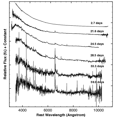
Figure 8: Kast and LRIS spectra of AT 2018cow over $t\simeq 2-59\,\mathrm{days}$, showing an initial featureless spectrum with emerging intermediate-width lines at $t\gtrsim 15\,\mathrm{days}$.

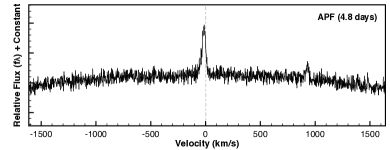
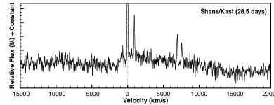
Figure 9: High-resolution APF and Kast spectra in velocity space centered at H$\alpha$ in rest frame relative to host redshift.

In the high-resolution APF spectrum taken at $t=4.77\,\mathrm{days}$, only narrow H$\alpha$ and [N II] $\lambda$6583 emission lines were resolved with a width of $v\sim 30-40\,\mathrm{km}\,\mathrm{s}^{-1}$ (see Figure 9). These narrow features are also blueshifted by $\sim$15 km s^-1 relative to the rest wavelength, consistent with the gas velocity at the site of AT 2018cow (see Figure 6 in Lyman et al., 2020). Therefore, the Levy spectrum confirms that no narrow lines from the transient existed at $t=4.77\,\mathrm{days}$ (and possibly for the first few days), as the detected lines are likely associated with the host galaxy.

Appendix B Dust Model for the Excess IR Emission

We introduced a model of the form blackbody + dust to test the robustness of the blackbody properties, i.e., whether or not they change if the power law is switched to a dust model.

We adopted a warm dust model assuming an ideal cloud of spherical dust grains with uniform size, composition, and temperature, with a flux density given by (Equation (4) of Hildebrand, 1983):

$$F_{\nu,\mathrm{d}}(M_{\mathrm{d}},T_{\mathrm{d}})=\frac{3Q_{\nu}(a)}{4\rho a}\frac{M_{\mathrm{d}}}{d_{\mathrm{L}}^{2}}B_{\nu}(T_{\mathrm{d}})$$ (B1)

where $Q_{\nu}(a)$ is the dust absorption coefficient, $\rho$ is the mass density of the grain, $a$ is the grain radius, $M_{\mathrm{d}}$ is the total mass of the dust cloud, and $T_{\mathrm{d}}$ is the temperature of the dust cloud. We assumed a fiducial dust size of of $a=0.1\,\mu\mathrm{m}$. We used the coefficients $Q_{\nu}(a)$ derived in Draine & Lee (1984) and Laor & Draine (1993) from Draine’s website. Generally, dust relevant for SNe is either graphite, with $\rho=2.26\,\mathrm{g}\,\mathrm{cm}^{-3}$, or silicate, with $\rho=3.30\,\mathrm{g}\,\mathrm{cm}^{-3}$. Therefore, there are two free parameters in the warm dust model: $M_{\mathrm{d}}$ and $T_{\mathrm{d}}$.

The total theoretical spectrum is then given by

$$f_{\nu} = F_{\nu,\mathrm{BB}}(R_{\mathrm{BB}},T_{\mathrm{BB}})+F_{\nu,\mathrm{d}}(M_{\mathrm{d}},T_{\mathrm{d}})$$ (B2)

$$= \frac{\pi R_{\mathrm{BB}}^{2}}{d_{\mathrm{L}}^{2}}B_{\nu}(T_{\mathrm{BB}})+\frac{3Q_{\nu}(a)}{4\rho a}\frac{M_{\mathrm{d}}}{d_{\mathrm{L}}^{2}}B_{\nu}(T_{\mathrm{d}}),$$

from which we obtain the best-fit $R_{\mathrm{BB}}$, $T_{\mathrm{BB}}$, $M_{\mathrm{d}}$, and $T_{\mathrm{d}}$ through our fitting procedure. For this test, to ensure that our results are well-constrained, we only fit the model to the six epochs with $JHK$ measurements. Initially, we attempted two separate fits: one for silicate dust and the other for graphite dust. However, the fits for silicate dust consistently produced $T_{\mathrm{d}}\sim 1700\,\mathrm{K}$, well above the evaporation temperature of silicate dust of $\sim 1100-1500\,\mathrm{K}$. Therefore, we did not further consider the case of silicate dust and only used the $Q_{\nu}(a)$ and $\rho$ values for graphite dust.

The observed SEDs with $JHK$ measurements, together with the best-fit models, are shown in Figure 10. We found that even with the dust model, the shape and amplitude of the UV-optical continuum are almost exclusively dictated by the blackbody. On the other hand, the dust model does provide a reasonable fit to the observed excess IR emission.

We also derived the bolometric luminosities for the blackbody + dust model. The luminosity of the blackbody was still calculated using Equation 2. The luminosity of the dust was taken as

$$L_{\mathrm{d}}=\frac{3\pi M_{\mathrm{d}}}{\rho a}\int_{0}^{\infty}Q_{\nu}B_{\nu}(T_{\mathrm{d}})d\nu.$$ (B3)

The best-fit parameters, bolometric luminosities, and the reduced chi-square $\chi^{2}/d.o.f$ from fitting the blackbody + dust model are given in Table 5. The derived dust temperature ($T_{\mathrm{d}}\sim 1100-1400\,\mathrm{K}$) is below the evaporation temperature of graphite ($\sim 1900\,\mathrm{K}$). The derived mass ($M_{\mathrm{d}}\sim 10^{-4}-10^{-6}$) also seems reasonable for SNe (e.g., see Gan et al., 2021, for Type Ibn SNe). The $\chi^{2}/\mathrm{d.o.f}$ values are also similar to those from the blackbody + power law model.

Most importantly, the thermal properties (i.e., temperature and radius) derived from the blackbody + dust fits are very similar to those derived from the blackbody + power law fits. Therefore, we conclude that the thermal properties derived from the blackbody are robust and reliable for our interpretations in this study regardless of the description of the excess IR emission.

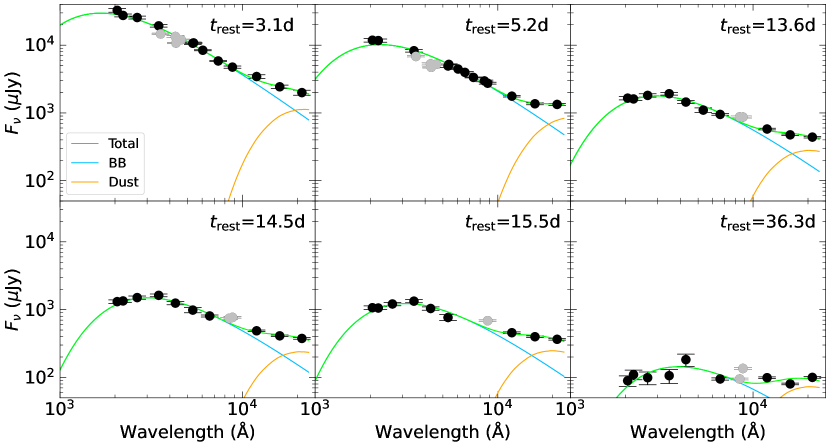
Figure 10: The observed (dereddened) SEDs of AT 2018cow (black circles) and the best-fit models (solid lines) derived from fitting the blackbody + dust model. The six chosen epochs all have JHK measurements that provide better constraints on the excess IR emission. Photometry excluded from the fit are shown in gray (see text for reasoning). The dust model generally provides a reasonable fit to the observed excess IR emission. More importantly, the UV-optical continuum from the is almost exclusively from the hot blackbody and unaffected by the dust model.

Table 5: Properties of AT 2018cow derived from the blackbody + dust model

$t\,(\mathrm{day})$	$R_{\mathrm{BB}}\,(R_{\odot})$	$T_{\mathrm{BB}}\,(\mathrm{K})$	$M_{\mathrm{d}}\,(10^{-5}\,M_{\odot})$	$T_{\mathrm{d}}\,(\mathrm{K})$	$L_{\mathrm{BB}}\,(10^{41}\,\mathrm{erg}\,\mathrm{s}^{-1})$	$L_{\mathrm{d}}\,(10^{41}\,\mathrm{erg}\,\mathrm{s}^{-1})$	$\chi^{2}/\mathrm{d.o.f}$
3.09	$11139.47^{+240.73}_{-251.08}$	$30513.00^{+911.27}_{-823.90}$	$13.99^{+13.30}_{-5.60}$	$1342.54^{+123.81}_{-132.48}$	$3707.85^{+286.10}_{-243.24}$	$8.42^{+1.05}_{-0.96}$	5.91
5.20	$10278.66^{+201.04}_{-208.99}$	$22545.53^{+545.90}_{-510.42}$	$23.06^{+10.82}_{-7.40}$	$1147.50^{+71.62}_{-64.67}$	$940.61^{+55.02}_{-48.99}$	$5.31^{+0.32}_{-0.30}$	4.61
13.56	$6436.58^{+178.68}_{-182.62}$	$17228.09^{+362.22}_{-339.02}$	$2.62^{+0.67}_{-0.48}$	$1420.19^{+56.79}_{-59.87}$	$125.94^{+4.27}_{-4.17}$	$2.14^{+0.12}_{-0.11}$	4.84
14.53	$6090.10^{+181.88}_{-183.84}$	$16852.33^{+357.73}_{-337.74}$	$2.50^{+0.62}_{-0.46}$	$1388.99^{+55.78}_{-55.98}$	$103.23^{+3.24}_{-3.26}$	$1.79^{+0.10}_{-0.10}$	2.62
15.54	$5773.85^{+320.69}_{-297.70}$	$16370.74^{+521.14}_{-503.43}$	$2.06^{+0.53}_{-0.39}$	$1454.01^{+65.78}_{-68.66}$	$82.60^{+2.75}_{-2.60}$	$1.93^{+0.16}_{-0.15}$	3.79
36.27	$2758.71^{+153.19}_{-151.79}$	$13083.00^{+568.79}_{-499.48}$	$0.70^{+0.13}_{-0.11}$	$1411.00^{+46.70}_{-46.02}$	$7.69^{+0.59}_{-0.50}$	$0.55^{+0.03}_{-0.02}$	25.89

. The degrees-of-freedom ($d.o.f$) is taken to be the number of data points minus the number of free model parameters.

Note. — Errors given here are statistical errors from the 15.9th and 84.1th percentile

References

- Arcavi et al. (2016) Arcavi, I., Wolf, W. M., Howell, D. A., et al. 2016, ApJ, 819, 35, doi: 10.3847/0004-637X/819/1/35
- Astropy Collaboration et al. (2013) Astropy Collaboration, Robitaille, T. P., Tollerud, E. J., et al. 2013, A&A, 558, A33, doi: 10.1051/0004-6361/201322068
- Astropy Collaboration et al. (2018) Astropy Collaboration, Price-Whelan, A. M., Sipőcz, B. M., et al. 2018, AJ, 156, 123, doi: 10.3847/1538-3881/aabc4f
- Becker (2015) Becker, A. 2015, HOTPANTS: High Order Transform of PSF ANd Template Subtraction. http://ascl.net/1504.004
- Bietenholz et al. (2020) Bietenholz, M. F., Margutti, R., Coppejans, D., et al. 2020, MNRAS, 491, 4735, doi: 10.1093/mnras/stz3249
- Bright et al. (2022) Bright, J. S., Margutti, R., Matthews, D., et al. 2022, ApJ, 926, 112, doi: 10.3847/1538-4357/ac4506
- Brooks et al. (2017) Brooks, J., Schwab, J., Bildsten, L., et al. 2017, ApJ, 850, 127, doi: 10.3847/1538-4357/aa9568
- Calderón et al. (2021) Calderón, D., Pejcha, O., & Duffell, P. C. 2021, MNRAS, 507, 1092, doi: 10.1093/mnras/stab2219
- Cardelli et al. (1989) Cardelli, J. A., Clayton, G. C., & Mathis, J. S. 1989, ApJ, 345, 245, doi: 10.1086/167900
- Chatzopoulos et al. (2012) Chatzopoulos, E., Wheeler, J. C., & Vinko, J. 2012, ApJ, 746, 121, doi: 10.1088/0004-637X/746/2/121
- Chen et al. (2023) Chen, Y., Drout, M. R., Piro, A. L., et al. 2023, arXiv e-prints, arXiv:2303.03501, doi: 10.48550/arXiv.2303.03501
- Cohen & Soker (2023) Cohen, T., & Soker, N. 2023, MNRAS, 522, 885, doi: 10.1093/mnras/stad1015
- Coppejans et al. (2020) Coppejans, D. L., Margutti, R., Terreran, G., et al. 2020, ApJ, 895, L23, doi: 10.3847/2041-8213/ab8cc7
- Dolphin (2016) Dolphin, A. 2016, DOLPHOT: Stellar photometry, Astrophysics Source Code Library, record ascl:1608.013. http://ascl.net/1608.013
- Draine & Lee (1984) Draine, B. T., & Lee, H. M. 1984, ApJ, 285, 89, doi: 10.1086/162480
- Drout et al. (2014) Drout, M. R., Chornock, R., Soderberg, A. M., et al. 2014, ApJ, 794, 23, doi: 10.1088/0004-637X/794/1/23
- Fang et al. (2019) Fang, K., Metzger, B. D., Murase, K., Bartos, I., & Kotera, K. 2019, ApJ, 878, 34, doi: 10.3847/1538-4357/ab1b72
- Filippenko (1982) Filippenko, A. V. 1982, PASP, 94, 715, doi: 10.1086/131052
- Flewelling et al. (2020) Flewelling, H. A., Magnier, E. A., Chambers, K. C., et al. 2020, ApJS, 251, 7, doi: 10.3847/1538-4365/abb82d
- Foreman-Mackey et al. (2013) Foreman-Mackey, D., Hogg, D. W., Lang, D., & Goodman, J. 2013, PASP, 125, 306, doi: 10.1086/670067
- Fox & Smith (2019) Fox, O. D., & Smith, N. 2019, MNRAS, 488, 3772, doi: 10.1093/mnras/stz1925
- Fujibayashi et al. (2022) Fujibayashi, S., Sekiguchi, Y., Shibata, M., & Wanajo, S. 2022, arXiv e-prints, arXiv:2212.03958, doi: 10.48550/arXiv.2212.03958
- Gan et al. (2021) Gan, W.-P., Wang, S.-Q., & Liang, E.-W. 2021, ApJ, 914, 125, doi: 10.3847/1538-4357/abfbdf
- Gehrels et al. (2004) Gehrels, N., Chincarini, G., Giommi, P., et al. 2004, ApJ, 611, 1005, doi: 10.1086/422091
- Gottlieb et al. (2022) Gottlieb, O., Tchekhovskoy, A., & Margutti, R. 2022, MNRAS, 513, 3810, doi: 10.1093/mnras/stac910
- Greene et al. (2020) Greene, J. E., Strader, J., & Ho, L. C. 2020, ARA&A, 58, 257, doi: 10.1146/annurev-astro-032620-021835
- Greiner et al. (2008) Greiner, J., Bornemann, W., Clemens, C., et al. 2008, PASP, 120, 405, doi: 10.1086/587032
- Hack et al. (2021) Hack, W. J., Cara, M., Sosey, M., et al. 2021, spacetelescope/drizzlepac: Drizzlepac v3.3.0, 3.3.0, Zenodo, Zenodo, doi: 10.5281/zenodo.5534751
- Hildebrand (1983) Hildebrand, R. H. 1983, QJRAS, 24, 267
- Hinkle et al. (2021) Hinkle, J. T., Holoien, T. W. S., Shappee, B. J., & Auchettl, K. 2021, ApJ, 910, 83, doi: 10.3847/1538-4357/abe4d8
- Ho et al. (2019) Ho, A. Y. Q., Phinney, E. S., Ravi, V., et al. 2019, ApJ, 871, 73, doi: 10.3847/1538-4357/aaf473
- Ho et al. (2020) Ho, A. Y. Q., Perley, D. A., Kulkarni, S. R., et al. 2020, ApJ, 895, 49, doi: 10.3847/1538-4357/ab8bcf
- Ho et al. (2022) Ho, A. Y. Q., Margalit, B., Bremer, M., et al. 2022, ApJ, 932, 116, doi: 10.3847/1538-4357/ac4e97
- Ho et al. (2023) Ho, A. Y. Q., Perley, D. A., Gal-Yam, A., et al. 2023, ApJ, 949, 120, doi: 10.3847/1538-4357/acc533
- Horne (1986) Horne, K. 1986, PASP, 98, 609, doi: 10.1086/131801
- Hotokezaka et al. (2017) Hotokezaka, K., Kashiyama, K., & Murase, K. 2017, ApJ, 850, 18, doi: 10.3847/1538-4357/aa8c7d
- Huang et al. (2019) Huang, K., Shimoda, J., Urata, Y., et al. 2019, ApJ, 878, L25, doi: 10.3847/2041-8213/ab23fd
- Inserra (2019) Inserra, C. 2019, Nature Astronomy, 3, 697, doi: 10.1038/s41550-019-0854-4
- Karamehmetoglu et al. (2021) Karamehmetoglu, E., Fransson, C., Sollerman, J., et al. 2021, A&A, 649, A163, doi: 10.1051/0004-6361/201936308
- Kashiyama & Quataert (2015) Kashiyama, K., & Quataert, E. 2015, MNRAS, 451, 2656, doi: 10.1093/mnras/stv1164
- Kawana et al. (2020) Kawana, K., Maeda, K., Yoshida, N., & Tanikawa, A. 2020, ApJ, 890, L26, doi: 10.3847/2041-8213/ab7209
- Khatami & Kasen (2023) Khatami, D., & Kasen, D. 2023, arXiv e-prints, arXiv:2304.03360, doi: 10.48550/arXiv.2304.03360
- Kilpatrick (2021) Kilpatrick, C. D. 2021, charliekilpatrick/hst123: hst123, v1.0.0, Zenodo, Zenodo, doi: 10.5281/zenodo.5573941
- Kilpatrick et al. (2018) Kilpatrick, C. D., Foley, R. J., Drout, M. R., et al. 2018, MNRAS, 473, 4805, doi: 10.1093/mnras/stx2675
- Kilpatrick et al. (2022) Kilpatrick, C. D., Fong, W.-f., Blanchard, P. K., et al. 2022, ApJ, 926, 49, doi: 10.3847/1538-4357/ac3e59
- Kleiser et al. (2018a) Kleiser, I., Fuller, J., & Kasen, D. 2018a, MNRAS, 481, L141, doi: 10.1093/mnrasl/sly180
- Kleiser et al. (2018b) Kleiser, I. K. W., Kasen, D., & Duffell, P. C. 2018b, MNRAS, 475, 3152, doi: 10.1093/mnras/stx3321
- Kremer et al. (2021) Kremer, K., Lu, W., Piro, A. L., et al. 2021, ApJ, 911, 104, doi: 10.3847/1538-4357/abeb14
- Krisciunas et al. (2017) Krisciunas, K., Contreras, C., Burns, C. R., et al. 2017, AJ, 154, 211, doi: 10.3847/1538-3881/aa8df0
- Kuin et al. (2019) Kuin, N. P. M., Wu, K., Oates, S., et al. 2019, MNRAS, 487, 2505, doi: 10.1093/mnras/stz053
- Kurfürst et al. (2020) Kurfürst, P., Pejcha, O., & Krtička, J. 2020, A&A, 642, A214, doi: 10.1051/0004-6361/202039073
- Laor & Draine (1993) Laor, A., & Draine, B. T. 1993, ApJ, 402, 441, doi: 10.1086/172149
- Leung et al. (2020) Leung, S.-C., Blinnikov, S., Nomoto, K., et al. 2020, ApJ, 903, 66, doi: 10.3847/1538-4357/abba33
- Liu et al. (2023) Liu, J.-F., Liu, L.-D., Yu, Y.-W., & Zhu, J.-P. 2023, ApJ, 946, 35, doi: 10.3847/1538-4357/acbb04
- Liu et al. (2022) Liu, J.-F., Zhu, J.-P., Liu, L.-D., Yu, Y.-W., & Zhang, B. 2022, ApJ, 935, L34, doi: 10.3847/2041-8213/ac86d2
- Liu et al. (2018) Liu, L.-D., Zhang, B., Wang, L.-J., & Dai, Z.-G. 2018, ApJ, 868, L24, doi: 10.3847/2041-8213/aaeff6
- Lyman et al. (2020) Lyman, J. D., Galbany, L., Sánchez, S. F., et al. 2020, MNRAS, 495, 992, doi: 10.1093/mnras/staa1243
- Lyutikov (2022) Lyutikov, M. 2022, MNRAS, 515, 2293, doi: 10.1093/mnras/stac1717
- Lyutikov & Toonen (2019) Lyutikov, M., & Toonen, S. 2019, MNRAS, 487, 5618, doi: 10.1093/mnras/stz1640
- Maeda & Moriya (2022) Maeda, K., & Moriya, T. J. 2022, ApJ, 927, 25, doi: 10.3847/1538-4357/ac4672
- Margalit (2022) Margalit, B. 2022, ApJ, 933, 238, doi: 10.3847/1538-4357/ac771a
- Margalit et al. (2022) Margalit, B., Quataert, E., & Ho, A. Y. Q. 2022, ApJ, 928, 122, doi: 10.3847/1538-4357/ac53b0
- Margutti et al. (2019) Margutti, R., Metzger, B. D., Chornock, R., et al. 2019, ApJ, 872, 18, doi: 10.3847/1538-4357/aafa01
- Maund et al. (2023) Maund, J. R., Höflich, P. A., Steele, I. A., et al. 2023, MNRAS, 521, 3323, doi: 10.1093/mnras/stad539
- McDowell et al. (2018) McDowell, A. T., Duffell, P. C., & Kasen, D. 2018, ApJ, 856, 29, doi: 10.3847/1538-4357/aaa96e
- Metzger (2022) Metzger, B. D. 2022, ApJ, 932, 84, doi: 10.3847/1538-4357/ac6d59
- Metzger & Perley (2023) Metzger, B. D., & Perley, D. A. 2023, ApJ, 944, 74, doi: 10.3847/1538-4357/acae89
- Michałowski et al. (2019) Michałowski, M. J., Kamphuis, P., Hjorth, J., et al. 2019, A&A, 627, A106, doi: 10.1051/0004-6361/201935372
- Miller & Stone (1993) Miller, J. S., & Stone, R. P. S. 1993, LOTRM
- Mohan et al. (2020) Mohan, P., An, T., & Yang, J. 2020, ApJ, 888, L24, doi: 10.3847/2041-8213/ab64d1
- Mor et al. (2023) Mor, R., Livne, E., & Piran, T. 2023, MNRAS, 518, 623, doi: 10.1093/mnras/stac2775
- Moriya & Eldridge (2016) Moriya, T. J., & Eldridge, J. J. 2016, MNRAS, 461, 2155, doi: 10.1093/mnras/stw1471
- Morokuma-Matsui et al. (2019) Morokuma-Matsui, K., Morokuma, T., Tominaga, N., et al. 2019, ApJ, 879, L13, doi: 10.3847/2041-8213/ab2915
- Nayana & Chandra (2021) Nayana, A. J., & Chandra, P. 2021, ApJ, 912, L9, doi: 10.3847/2041-8213/abed55
- Ofek et al. (2010) Ofek, E. O., Rabinak, I., Neill, J. D., et al. 2010, ApJ, 724, 1396, doi: 10.1088/0004-637X/724/2/1396
- Oke et al. (1995) Oke, J. B., Cohen, J. G., Carr, M., et al. 1995, PASP, 107, 375, doi: 10.1086/133562
- Onken et al. (2019) Onken, C. A., Wolf, C., Bessell, M. S., et al. 2019, PASA, 36, e033, doi: 10.1017/pasa.2019.27
- Pasham et al. (2021) Pasham, D. R., Ho, W. C. G., Alston, W., et al. 2021, Nature Astronomy, 6, 249, doi: 10.1038/s41550-021-01524-8
- Pellegrino et al. (2022) Pellegrino, C., Howell, D. A., Vinkó, J., et al. 2022, ApJ, 926, 125, doi: 10.3847/1538-4357/ac3e63
- Perley et al. (2019) Perley, D. A., Mazzali, P. A., Yan, L., et al. 2019, MNRAS, 484, 1031, doi: 10.1093/mnras/sty3420
- Perley et al. (2021) Perley, D. A., Ho, A. Y. Q., Yao, Y., et al. 2021, MNRAS, 508, 5138, doi: 10.1093/mnras/stab2785
- Piro & Lu (2020) Piro, A. L., & Lu, W. 2020, ApJ, 894, 2, doi: 10.3847/1538-4357/ab83f6
- Prentice et al. (2016) Prentice, S. J., Mazzali, P. A., Pian, E., et al. 2016, MNRAS, 458, 2973, doi: 10.1093/mnras/stw299
- Prentice et al. (2018) Prentice, S. J., Maguire, K., Smartt, S. J., et al. 2018, ApJ, 865, L3, doi: 10.3847/2041-8213/aadd90
- Pursiainen et al. (2018) Pursiainen, M., Childress, M., Smith, M., et al. 2018, MNRAS, 481, 894, doi: 10.1093/mnras/sty2309
- Quataert et al. (2019) Quataert, E., Lecoanet, D., & Coughlin, E. R. 2019, MNRAS, 485, L83, doi: 10.1093/mnrasl/slz031
- Rest et al. (2005) Rest, A., Stubbs, C., Becker, A. C., et al. 2005, ApJ, 634, 1103, doi: 10.1086/497060
- Rest et al. (2018) Rest, A., Garnavich, P. M., Khatami, D., et al. 2018, Nature Astronomy, 2, 307, doi: 10.1038/s41550-018-0423-2
- Rivera Sandoval et al. (2018) Rivera Sandoval, L. E., Maccarone, T. J., Corsi, A., et al. 2018, MNRAS, 480, L146, doi: 10.1093/mnrasl/sly145
- Roming et al. (2005) Roming, P. W. A., Kennedy, T. E., Mason, K. O., et al. 2005, Space Sci. Rev., 120, 95, doi: 10.1007/s11214-005-5095-4
- Roychowdhury et al. (2019) Roychowdhury, S., Arabsalmani, M., & Kanekar, N. 2019, MNRAS, 485, L93, doi: 10.1093/mnrasl/slz035
- Schlafly & Finkbeiner (2011) Schlafly, E. F., & Finkbeiner, D. P. 2011, ApJ, 737, 103, doi: 10.1088/0004-637X/737/2/103
- Scolnic et al. (2015) Scolnic, D., Casertano, S., Riess, A., et al. 2015, ApJ, 815, 117, doi: 10.1088/0004-637X/815/2/117
- Shivvers et al. (2016) Shivvers, I., Zheng, W. K., Mauerhan, J., et al. 2016, MNRAS, 461, 3057, doi: 10.1093/mnras/stw1528
- Siebert et al. (2019) Siebert, M. R., Foley, R. J., Jones, D. O., et al. 2019, MNRAS, 486, 5785, doi: 10.1093/mnras/stz1209
- Smartt et al. (2018) Smartt, S. J., Clark, P., Smith, K. W., et al. 2018, The Astronomer’s Telegram, 11727, 1
- Smith & Nelson (1969) Smith, C. E., & Nelson, B. 1969, PASP, 81, 74, doi: 10.1086/128742
- Smith et al. (2018) Smith, P. S., Leonard, D. C., Bilinski, C., et al. 2018, The Astronomer’s Telegram, 11789, 1
- Soker (2022) Soker, N. 2022, Research in Astronomy and Astrophysics, 22, 055010, doi: 10.1088/1674-4527/ac5b40
- Soker et al. (2019) Soker, N., Grichener, A., & Gilkis, A. 2019, MNRAS, 484, 4972, doi: 10.1093/mnras/stz364
- Steele et al. (2004) Steele, I. A., Smith, R. J., Rees, P. C., et al. 2004, in Society of Photo-Optical Instrumentation Engineers (SPIE) Conference Series, Vol. 5489, Ground-based Telescopes, ed. J. Oschmann, Jacobus M., 679–692, doi: 10.1117/12.551456
- Sun et al. (2022) Sun, N.-C., Maund, J. R., Crowther, P. A., & Liu, L.-D. 2022, MNRAS, 512, L66, doi: 10.1093/mnrasl/slac023
- Sun et al. (2023) Sun, N.-C., Maund, J. R., Shao, Y., & Janiak, I. A. 2023, MNRAS, 519, 3785, doi: 10.1093/mnras/stac3773
- Suzuki et al. (2019) Suzuki, A., Moriya, T. J., & Takiwaki, T. 2019, ApJ, 887, 249, doi: 10.3847/1538-4357/ab5a83
- Suzuki et al. (2020) —. 2020, ApJ, 899, 56, doi: 10.3847/1538-4357/aba0ba
- Tampo et al. (2020) Tampo, Y., Tanaka, M., Maeda, K., et al. 2020, ApJ, 894, 27, doi: 10.3847/1538-4357/ab7ccc
- Tanaka et al. (2016) Tanaka, M., Tominaga, N., Morokuma, T., et al. 2016, ApJ, 819, 5, doi: 10.3847/0004-637X/819/1/5
- Tolstov et al. (2019) Tolstov, A., Nomoto, K., Sorokina, E., et al. 2019, ApJ, 881, 35, doi: 10.3847/1538-4357/ab2876
- Tsuna et al. (2021) Tsuna, D., Kashiyama, K., & Shigeyama, T. 2021, ApJ, 922, L34, doi: 10.3847/2041-8213/ac3997
- Uno & Maeda (2020) Uno, K., & Maeda, K. 2020, ApJ, 897, 156, doi: 10.3847/1538-4357/ab9632
- Virtanen et al. (2020) Virtanen, P., Gommers, R., Oliphant, T. E., et al. 2020, Nature Methods, 17, 261, doi: 10.1038/s41592-019-0686-2
- Vogt et al. (2014) Vogt, S. S., Radovan, M., Kibrick, R., et al. 2014, PASP, 126, 359, doi: 10.1086/676120
- Wang et al. (2019) Wang, L. J., Wang, X. F., Cano, Z., et al. 2019, MNRAS, 489, 1110, doi: 10.1093/mnras/stz2184
- Wang & Gan (2022) Wang, S.-Q., & Gan, W.-P. 2022, ApJ, 928, 114, doi: 10.3847/1538-4357/ac53aa
- Wang & Li (2020) Wang, S.-Q., & Li, L. 2020, ApJ, 900, 83, doi: 10.3847/1538-4357/aba6e9
- Whitesides et al. (2017) Whitesides, L., Lunnan, R., Kasliwal, M. M., et al. 2017, ApJ, 851, 107, doi: 10.3847/1538-4357/aa99de
- Wiseman et al. (2020) Wiseman, P., Pursiainen, M., Childress, M., et al. 2020, MNRAS, 498, 2575, doi: 10.1093/mnras/staa2474
- Xiang et al. (2021) Xiang, D., Wang, X., Lin, W., et al. 2021, ApJ, 910, 42, doi: 10.3847/1538-4357/abdeba
- Yao et al. (2022) Yao, Y., Ho, A. Y. Q., Medvedev, P., et al. 2022, ApJ, 934, 104, doi: 10.3847/1538-4357/ac7a41
- Yu et al. (2019) Yu, Y.-W., Chen, A., & Li, X.-D. 2019, ApJ, 877, L21, doi: 10.3847/2041-8213/ab1f85
- Yu et al. (2015) Yu, Y.-W., Li, S.-Z., & Dai, Z.-G. 2015, ApJ, 806, L6, doi: 10.1088/2041-8205/806/1/L6