Partial-Information, Longitudinal Cyber Attacks on Sensing in Autonomy

Abstract

Reports from the traffic safety authorities cite the concerning increase in cyber attacks on vehicles. However, security analyses tend to focus either on cyber threats that pose minimal safety-critical concern (e.g., door unlocking) or safety-relevant attacks that are exercised through physical channels. In this work, we present and evaluate cyber threats against safety-critical sensing in autonomous vehicles (AVs). Our novel threat model is a cyber-level attacker capable of disrupting sensor data via malware at the firmware/driver level. Uniquely, our attacker will lack any situational awareness and direct access to the AV algorithms. Even with only access to raw sensor data from a single sensor, an attacker can design attacks that critically compromise downstream perception and tracking in multi-sensor AVs. To mitigate vulnerabilities, we introduce two improvements for security-aware sensor fusion: a probabilistic data-asymmetry monitor and a scalable track-to-track fusion of 3D LiDAR and monocular detections (T2T-3DLM); we demonstrate that the approaches significantly reduce attack effectiveness.

1 Introduction

A recent report from the National Highway Traffic Safety Administration (NHTSA) described the concerning increase in remote exploitation of vehicle hardware and software [42]. The investment in new technologies such as connected vehicles is meant to promote improved efficiency of travel and mitigate safety risks. Unfortunately, it coincides with a dramatic rise in cyber threats against cyber physical systems (CPS) [58]. Recent attacks on vehicles underscore the vulnerability that comes with an increase in demand for cross-module integration and advanced driving features [15]. Through attack vectors including physical access to vehicle components, remote access through a number of wireless interfaces, compromised over-the-air (OTA) software updates, and supply-chain infiltration, the automotive attack surface is large.

With access to a vehicle through the automotive attack surface, there are a number of forms an attack can take. One important class of attacks is code injection attacks against device firmware and drivers. Recent examples highlight the prevalence of such attacks with many vehicle subsystems subject to firmware injection. However, thus far, many examples of firmware injection attacks were not safety-critical; many proved to be “nuisances” that, e.g., compromised the in-vehicle-infotainment (IVI) system [40, 39, 38, 37] or drained the vehicle’s battery when it was parked [15].

Since vehicle lifetime is over a decade, it is only a matter of time before firmware injection attacks succeed on safety-critical subsystems. One such avenue for safety-critical impact is to target sensors in autonomous vehicles (AVs). Safety-critical AV sensors include cameras, LiDAR, and radar providing the information that forms an AV’s situational awareness. These sensors are safety-critical because an AV uses its situational awareness to plan a safe path through a complex environment filled with moving obstacles at high speeds.

In an effort to proactively identify the capability of a cyber-level attacker compromising safety-critical sensing in AVs, we consider a cyber threat where the sensor data relayed from the sensor to the computation subsystem in an AV is compromised by malware that modifies the sensing data in real-time. In such a general threat model for cyber-based sensor attacks, only partial AV information is available to the attacker; i.e., the attacker has nearly no information about the AV itself, its surroundings (environment), or data from other sensors before and during the attack since the attacker is only compromising the sensor firmware. We first describe general principles of cyber threats on sensors. We then apply these principles to the case of a compromised LiDAR sensor due to the importance of LiDAR in 3D object perception for AVs.

Despite the attacker’s limited knowledge, we find that multiple successful cyber attack implementations targeting LiDAR exist. We derive eight attacks in total. Four require no information on the environment (“context-unaware”); these are the false positive, dual false positive, forward replay, and reverse replay attacks. Four require the attacker to induce some situational awareness from only the raw LiDAR data online (“context-aware”); these are the clean-scene, object removal, frustum translation, and dual frustum false positive attacks. All attacks remain stealthy to basic data integrity checks that follow from LiDAR point-cloud structure.

We establish that, for attacks on AV sensors to create impactful outcomes, they must satisfy the following: 1) Perception: Must create detection outcomes at the perception level; 2) Longitudinal: Must propagate temporally at object tracking; and 3) Safety-Critical: Must create safety-critical changes to the scene or the vehicle’s awareness at the prediction and control levels. Recent AV security studies of sensor vulnerabilities presented limited analysis if the attacks led to measurable outcomes at all three levels. In particular, they have only focused on parts of the story; e.g., isolated attacks on single-frame sensor data [9, 49, 19, 50] or full scenes to show that attacks on perception can propagate longitudinally (i.e., over time) [19, 53, 8]. Few have illustrated such longitudinal effects cause measurable safety-critical incidents.

To test attacks on relevant AVs with realistic sensor data, we evaluate in simulation and on longitudinal datasets. In simulation, we employ the industry-grade Baidu Apollo self-driving software. On datasets, we use four representative AV implementations built from AVstack [20], the open-source AV development platform. The first two AVstack implementations are: (AV-1) LiDAR-based, and (AV-2) centralized camera-LiDAR fusion; both are based on common self-driving architectures (e.g., Baidu’s Apollo [3] and Autoware [2]) and are implemented with open-source algorithms [30, 43, 55, 28]. Recently, AV-1 and AV-2 were shown vulnerable to physical and white-box attacks [9, 49, 19, 50]. Hence, to improve the robustness of camera-LiDAR fusion to single-sensor-attacks, we extend AV designs with security awareness. Design (AV-3) builds on AV-2 and computes an agreement metric between data from multiple sensors to identify inconsistencies. Finally, design (AV-4) is motivated by the frustum attack [19]: we cast sensor fusion as a decentralized problem and design a track-to-track fusion (T2T) of 3D LiDAR and monocular data (3DLM) (T2T-3DLM) to mitigate 2D camera ambiguities.

We show that Baidu’s industry-grade Apollo driving software is vulnerable to even context-unaware partial-information cyber attacks. The attacker achieves emergency braking or collision outcomes for all cases when running LiDAR-based perception and camera-LiDAR fusion perception in Apollo 7.0. On longitudinal scenes from KITTI [16] and nuScenes [6], we once again find LiDAR-based perception and centralized camera-LiDAR fusion are vulnerable. The false positive attack has nearly 99% and 40% success generating safety-critical incidents against AV-1 and AV-2, respectively, while the context-aware frustum translation attack improves the success in AV-2 to 60%. Replay-type attacks have strong success with the reverse replay demonstrating nearly 50% success against AV-1 and AV-2 in generating safety-critical incidents with absolutely no prior knowledge and no context – simply buffering and replaying scene data.

However, despite compromised perception, the security-enhanced AV designs we introduce in this work (AVs-3,4) mitigate the propagation of attack traces at object-tracking. AV-3 reduces false positive attack success to less than 30% and replay attack success to less than 20%. At the safety-level, only AV-4 (T2T-3DLM) successfully mitigates the safety-critical outcomes of all tested attacks, showing that it can be used to add robustness against the cyber attacks on LiDAR sensing. Videos of the experiments are available at [1].

Contributions. The contributions of this work are:

• Motivate the need for an analysis of cyber attacks on safety-critical sensing in autonomous vehicles.

• Derive a realistic threat model for a cyber attacker that captures the limited knowledge, capabilities, and stealthiness constraints of a firmware injection attack.

• Implement the first successful LiDAR attacks in multi-sensor AVs with a limited-information cyber threat.

• Propose fusion-level defenses: a probabilistic measure of data-asymmetry/consistency between sensors and a track-to-track fusion of distributed monocular camera and LiDAR sensing for security-aware fusion.

• Evaluate five attacks against LiDAR on industry-grade AVs in simulation and representative AVs on longitudinal datasets through case studies and large-scale evaluations.

2 Background on Threat Model and Security

We first present recent high-profile evidence that cyber threats in vehicles are important for security research. We then identify the threats most likely to have safety-critical impact in AVs. Finally, we provide a summary of the most relevant security analyses for our selected attack vector.

2.1 Cyber Attack Vectors in AVs

To execute a cyber attack on vehicles, the attacker needs to infiltrate the system. Several cyber attack vectors have been demonstrated on vehicles over the past decade.

2.1.1 Physical access.

One vector for a cyber attack is to obtain physical access to the vehicle’s electronic components. Physical access was used in recent CPS security case studies [5, 29, 27, 23, 11]. Of particular concern for physical vulnerability in vehicles is the On-Board Diagnostic II (OBD-II) port. Indoctrinated in standard SAE J1962, all vehicles are required to use OBD-II to transmit emissions data. Many manufacturers also use OBD-II as a diagnostic and system-reprogramming interface [33]. This port directly connects onboard computers via the CAN bus. Clearly, unauthorized access to the OBD-II port would allow an adversary to transmit malicious messages or perform unauthorized device flashing.

2.1.2 Remote access.

Another attack vector is to leverage the increasing number of wireless interfaces to third-party entities. The investment in connected vehicle technologies such as vehicle-to-vehicle (V2V) and vehicle-to-infrastructure (V2I) is meant to promote improved efficiency of travel and mitigate safety risks. Unfortunately, it coincides with a dramatic rise in remote threats against CPS [58]. Recent case studies illustrate that connection between human-vehicle systems over Bluetooth/WiFi and V2V/V2I over cellular/WiFi for collaborative autonomy can lead to unauthorized remote access [17, 29, 11, 48, 52].

2.1.3 Over-the-air (OTA) updates.

Embedded software originates from human developers who inevitably introduce errors into firmware and application code. With hundreds of ECUs, millions of object code instruction, and gigabytes of software in a modern vehicle, software bugs are commonplace [14]. The rush to deploy AVs to market means more bugs in software. To address bugs rapidly and automatically, manufacturers increasingly prefer pushing updates OTA instead of recalling vehicles for physical updates [33].

2.1.4 Supply-chain infiltration.

The supply chain for vehicle components is a complex hierarchy composed of many original equipment manufacturers (OEMs). Each OEM may introduce critical features such as cryptographic keys, digital rights management, and proprietary firmware [33]. Moreover, as complex hardware pertinent to AVs proliferates, it becomes increasingly likely that third-party components such as sensors will be returned to the OEM or a third-party for maintenance. Without proper integrity validation, a single malicious actor in the vehicle supply chain can be the attack vector.

2.2 Cyber Attack Methodology

With access to a vehicle via an above vector, there are several ways an attack can be executed. Each methodology provides a unique capability and knowledge model.

2.2.1 CAN bus messaging.

A popular attack on vehicles is to manipulate controller area network (CAN) bus messages. CAN-bus messages are broadcast over the network, permitting anyone to sniff packets. Moreover, CAN-bus messages tend not to perform sender authentication. This was recently exploited by sending falsified control signals [17]. A similar vulnerability was discovered in the BlueDriver diagnostic system that allowed external devices to send CAN-bus messages [37]. Thus, to secure safety-critical systems against CAN-bus attacks, modern vehicles prevent access to critical subsystems (e.g., powertrain and automated driving) over the widely-accessible D-bus port of the CAN-bus. This renders attacks on control such as from [17] unlikely today [33].

2.2.2 Sybil/man-in-the-middle attack.

With a Sybil attack, an agent impersonates the identify of other agents in a peer-to-peer network. A malicious node acts as a man-in-the-middle to intercept legitimate traffic, manipulate message contents, and resend to the intended destination. Such an attack was demonstrated in vehicles to manipulate timing on V2V/V2I messages and cause out-of-date situational awareness [48].

2.2.3 Firmware/driver code injection.

Another class of attacks manipulates firmware and/or driver code. For example, one attack is to reverse-engineer existing firmware, apply a malicious perturbation, and reflash the device with the new firmware. Recently, vulnerabilities in Hyundai’s Gen5W and Tesla’s Model 3 in-vehicle-infotainment (IVI) systems allowed attackers to install custom IVI firmware [40, 39]. Additionally, an issue was discovered in the Tesla Model S IVI system that allowed attackers to send custom messages by compromising application drivers [38].

2.3 Likely Safety-Critical Cyber Attacks

Unlike most consumer-grade CPS, vehicles are meant to remain in their operational environment for over a decade. This allows adversaries plenty of time to apply promising attack vectors to new vehicles. Increasingly complex software requirements with continuously expanding component supply chains make adversarial OTA updates and supply chain infiltration particularly likely attack vectors in the near-term.

Leveraging these vectors, a promising class of attacks on AVs is firmware code injection. To achieve safety-critical impact in AVs, one attractive option is to target the firmware of sensing subsystems. Although it would be most impactful to e.g., directly attack perception or control algorithms, firmware injection is nearly impossible on the AV computation stack since algorithms for automated driving are proprietary and closed-source. On the other hand, sensors are a target for attacks because their firmware and drivers are released online, open-source. Sensing subsystems are more fruitful targets than other subsystems such as IVI because sensing has a direct bearing on a vehicle’s situational awareness.

2.4 Existing Safety-Critical Attacks on Sensing

We provide an overview of contemporary examples of safety-critical attacks on sensing. Prior analysis on sensing focuses on black-box attacks through physical channels and white-box attacks with access to model parameters (e.g., neural network weights). Until now, no work pursued limited-information cyber attacks on sensing. Table I summarizes attacks and differences from our work.

Several works use a LiDAR spoofing model to attack perception in AVs; e.g., [9, 46] established structured spoofing attacks that led to security studies capitalizing on white-box optimization [9], occlusion relationships [49], and ambiguities in multi-sensor fusion [19]. Other works use adversarial patches [50], physical adversarial objects [8] or road markings [44], designed from shape and texture optimization with white-box model access.

Attack	Threat Model	Attacker’s Knowledge	Demonstrated Capability	Assumed Capability
AdvLiDAR [9]	Spoofing	White-Box	Insert 60 points	Precise laser aiming w/ white-box.
BlackBox [49]	Spoofing	Black-Box	Insert 200 points	Precise laser aiming in pattern of a car.
Frustum [19]	Spoofing	Black-Box	Insert 200 points	Precise laser aiming.
AdvRoof [50]	Physical Adv. Object	White-Box	Gradient-based adv. object	White-box model access, large adv. obj.
MSF-Adv [8]	Physical Adv. Object	White-Box	Gradient-based adv. object	White-box model access.
DirtyRoad [44]	Physical Adv. Object	White-Box	Gradient-based dav. object	White-box model access.
Cyber Attack (this work)	Malware on Sensor, Comms, or Processing substrate	Incoming LiDAR point cloud only	Deriving situational awareness from point cloud online	Computational and memory capability

TABLE I: Existing state of the art attacks (top) fall into spoofing and physical-adversarial object categories with white and black-box flavors. All require either precise laser aiming or white-box model access. Ours (bottom) is the first to consider an increasingly-likely cyber threat model with nearly no information about the system and the environment of the vehicle.

2.4.1 Summary

We motivated a cyber threat against sensing in AVs through, e.g., a firmware injection attack. In Section 3, we describe the cyber threat against sensors including the attacker’s knowledge and capability. In Section 4, we describe attack implementations targeting LiDAR.

3 Cyber Attack Model

We now establish the model for partial-information cyber attacks. We motivated the threat model and discussed the feasibility of exercising this attack in the real world in Section 2. Here, we discuss the knowledge, constraint, and capability models of the attacker.

3.1 Limited Information Assumption

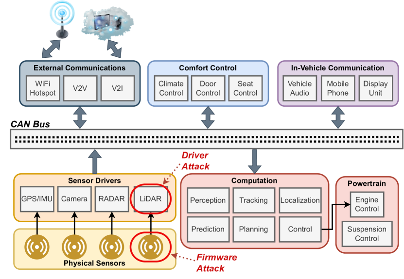
Figure 1: The automotive architecture provides connectivity of diverse services over mainly CAN bus. Attacks at the firmware/driver levels will only have access to isolated information at each subsystem.

An attack at the firmware or driver level of an AV’s sensing subsystem will have no access to information at other subsystems or from the environment other than the raw sensor data itself. This cyber threat model is illustrated in Figure 1. The sensing subsystem is compromised, and since information flows ‘downhill’ to the computation subsystem, the attacker is left without an ability to observe any downstream data. This limited-information model is in contrast to white-box attackers that assume knowledge of the perception model (e.g., neural network model weights) with control over sensor inputs (e.g., adversarial objects [8], image patches [24]). Such full-information attacks have yet to see relevance in real-world cases. The cyber model is also in contrast to “black-box” spoofing that assumes full environmental knowledge/situational awareness [19] and the ability to precisely aim a laser at a moving vehicle’s sensing array [9, 49].

3.2 Attacker Model

We now establish the attacker’s knowledge and capability within partial-information cyber attacks on AV sensors. We first address what information the attacker will have ahead of time. We then address what information the attacker can induce by observing sensor data (sent via compact datagrams) in real-time. Then, we consider an attack against the LiDAR sensor and discuss the constraints the attacker must operate under in this cyber context before establishing the capability of the attacker.

3.2.1 A-Priori Information

With a cyber attack at the sensor level, the attacker will have very little access to system or environment information. In fact, we only assume the following for a sensor attacker:

1. The attacker knows the size & structure of datagrams.

2. Each datagram is sent with timestamp information.

3. The attacker has basic configuration information on the sensor such as resolution and field of view.

4. Sensor is mounted with two axes coplanar to ground.

The attacker can obtain this information under the compromised firmware model. Other information (e.g., sensor height, presence of other sensors, runtime data, surrounding environment) is not known to the attacker.

3.2.2 Induced Information

Given the attacker’s access to incoming sensor data, the attacker can induce some information at runtime. For example, the attacker can easily compute the rate of the sensor by monitoring datagram timestamps. The attacker may be able to compute higher-order information with some additional effort and some uncertainty. This could include the sensor’s yaw angle offset from the vehicle’s forward direction or the sensor’s height from the ground (see Appendix A.1.2). We assume the attacker does not have any scene-specific information that would provide immediate situational awareness (e.g., object locations). The attacker is only capable of observing the incoming sensor data over time and estimating for herself. This is in contrast to prior works (e.g., [19]) that assumed a degree of accurate situational awareness a-priori.

3.2.3 Attacker’s Capabilities Targeting LiDAR

Due to the importance of LiDAR in safety-critical 3D object perception, the remainder of this work considers an attacker targeting a LiDAR sensor. Similar analysis can be performed for other sensors including cameras and radar.

3.2.4 Datagram Structure for Integrity

LiDAR data are sent to the computation subsystem following Figure 1 in compact datagrams. The datagram structure is consistent across sensors between a vendor; this provides a constraint over the attacker’s capability: if the attacker violates the datagram structure, the attack will be detected. We introduce simple, first-order integrity functions to validate common-sense characteristics of LiDAR data for the victim. The mathematical details of the integrity functions are presented in Appendix B.3.

1. Max Points: With the number of azimuth and elevation firing angles known a-priori, there is a hard upper bound on the number of returned points.

2. Min Points: With an expected success rate observed from testing, there is a soft lower bound on the number of returned points.

3. Timestamp: With a fixed rate of rotation/capture, there is a hard upper bound on the number of datagrams and the difference in their timestamps.

4. Dual: If the sensor is in dual mode, an angle’s second return will have a larger range than the first.

3.2.5 Stealthy capability.

The attacker can perform at least the following operations to the raw datagrams via the compromised firmware; these are stealthy to first-order integrity.

1. Range modification: Modify range in the datagrams.

2. Range nullification: Set some range entries to NULL.

3. Range spoofing: Set NULL range entries in the datagram to some floating point values.

4. Timestamp modification: Very subtly modify the timestamp field of the datagram.

5. Mode manipulation + spoofing: Switch mode from single to dual and add fake points.

6. Mode manipulation + dropping: Switch mode from dual to single and drop points.

7. Drop datagrams: Drop datagrams, acting like a data sinkhole for denial of service.

8. Add datagrams: Send additional (fake) datagrams.

Notably, the attacker cannot modify the azimuth or elevation angles of the returns (outside of using SC.4, small changes in timing) due to the datagrams’ rigid structure.

Importantly, some falsified LiDAR point clouds are easily detectable under first-order integrity. For example, given the minimum point requirement, the attacker’s capability SC.2 should not nullify a large number of LiDAR points. Similarly, the capability SC.4 should be used to only subtly modify the timestamps, otherwise it will fail the timestamp check. The use of  SC.5 must also be consistent with the dual verification check. Also, dropping (SC.7) or adding (SC.8) datagrams would be easily detected by monitoring datagram timestamp fields.

3.2.6 Auxiliary operations.

Finally, we assume the attacker can perform auxiliary operations to assist in the attack.

1. Preload: The attacker’s malware is instantiated with any pre-computed data tables she may desire.

2. Buffering: The attacker can buffer up sensor data into memory. Our most memory-intensive attack, the replay attack, requires no more than 10 MB of memory.

3. Compute: Some attacks require that the attacker run algorithms such as light-weight perception. For a resource-constrained, on-board environment, this could be a bird’s-eye-view clustering or use TinyML [31].

Future works will constrain these assumptions to the specifications of target hardware. In this first exploration, we put more emphasis on limiting the attacker’s knowledge.

4 Attack Designs With Limited Information

We design attacks from the attacker knowledge and capability introduced in Sec. 3. Some attacks require situational awareness (“context-aware”); we demarcate these requirements. This is as opposed to “context-unaware” attacks that do not require situational awareness.

4.1 Promising Attacks

The attacker capabilities and knowledge model introduced in Sec. 3 enable the following attacks that are stealthy to first-order receiver integrity from Sec. 3.2.3.

Context-unaware attacks:

1. False Positive: Manipulate the range entries within a subset of the angles (i.e., $(\theta_{i},\ \phi_{j})$ pairs) into some desired shape that is likely to be detected as an object by the AV.

2. False Positive (Dual): Change the mode bit from single to dual. Duplicate datagrams and manipulate the second copy, staying consistent with integrity INT.4.

3. Forward Replay: Duplicate existing datagrams; store the copy in a buffer. After some delay, attack by replaying from the buffer with consistent timestamps.

4. Reverse Replay: ATT.3, but in reverse order.

Context-aware attacks (with situational awareness):

1. Clean-Scene: Monitor the range of each $(\theta_{i},\ \phi_{j})$ pair. Find ranges that change between frames (e.g., may be an object). Replace those with ranges such that no object will be detected (i.e., act as ‘background’ ranges).

2. Object Removal: Determine which $(\theta_{i},\ \phi_{j})$ pairs encapsulate an object. Over these angles, replace the range entries with estimated background ranges.

3. Frustum Translation: Determine which $(\theta_{i},\ \phi_{j})$ pairs encapsulate an object. Over these angles, apply a shift function to points to translate the object forward or backward within the frustum (see Fig. 15, Appendix A.2);

4. Frustum False Positive (Dual): Determine which $(\theta_{i},\ \phi_{j})$ pairs encapsulate an object. Change the mode from single to dual. Duplicate datagrams and use the second copy for a false positive behind the true object.

We do not evaluate all proposed attacks in this work. More scrutiny is needed for attacks using the dual mode; while an attack in [19] assumed the LiDAR was in dual mode, this mode is not common in AVs. Thus, we do not consider attacks ATT.2 and ATT.8 as they rely on mode manipulation, nor do we consider clean scene attack ATT.5 since finding a tractable monitoring solution requires further effort.

Hence, from the context-unaware attacks, we consider the false positive ATT.1, forward replay ATT.3, and reverse replay ATT.4 attacks. From the context-aware attacks, we consider the object removal ATT.6 and frustum translation ATT.7 attacks. These attacks are well-motivated from prior security studies; ATT.1 is a cyber-realization of [9, 49]; replay attacks have been studied in the estimation and controls (e.g., [41, 36]); and ATT.7 borrows ideas from [19].

4.2 Practical Considerations

We test attacks on datasets and simulators rather than with a physical sensor, as LiDAR sensors are prohibitively expensive. The most affordable sensor, the Velodyne Puck, is only a 16-line scanner, which is not representative of self-driving applications that commonly employ 32 or 64 line scanners. The Velodyne HDL-32E and HDL-64E, on the other hand, cost upwards of $\$30,000$ and $\$75,000$, prohibitively expensive for accessible research. Using datasets and simulators instead of a physical LiDAR requires additional preprocessing to ensure the attacker’s knowledge is consistent with real-world attacks. These minor details are described in Appendix B.

4.3 Attack Implementations

We partition the attacker’s decision process into three sequential modules, executed at every time step:

1. Monitor: Gain insight on scene details (e.g., ground plane, objects) from raw sensor (i.e., LiDAR) data.

2. Schedule: Use monitoring information to plan attack over both spatial and temporal dimensions.

3. Execute: Compose attack operations against LiDAR data to best instantiate the scheduled plan.

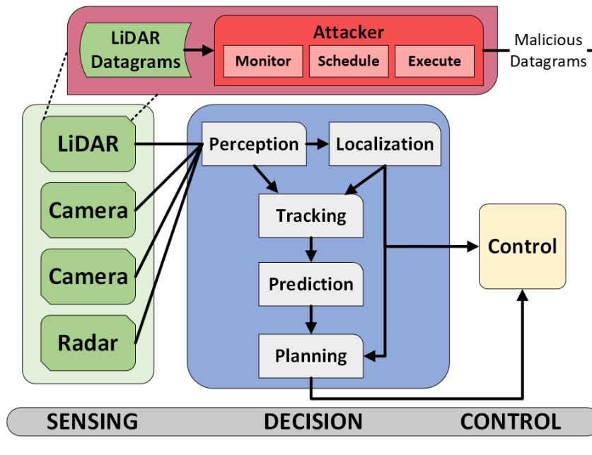
Figure 2: Even compromising only LiDAR data percolates through AV pipeline despite the multiple sensors’ data use. Incoming data packets are the attacker’s only knowledge.

Such attacks take the form summarized in Fig. 2 with the LiDAR data singularly compromised and the incoming data packets the attacker’s only knowledge. We now describe how to implement each attack module (Monitor, Schedule, Execute) for each of the five selected attacks.

4.3.1 Monitor

Many attacks benefit from monitoring LiDAR data; the attacker has no prior information and must obtain any situational awareness from monitoring. Monitoring can aid in the placement of attacks for maximum impact. It can also serve to trigger attack start at a favorable time.

Sensor Height/Ground Plane
The height of the sensor is not assumed to be known to the attacker. For attacks introducing false objects, it is helpful to know the sensor height (equivalently: the ground plane) to ensure points obey physical laws. By monitoring the LiDAR datagrams, the attacker can obtain an accurate estimate of the height of the sensor with simple geometry. A candidate monitoring algorithm is described in Appendix A.1.2.

Object Detection
Context-aware attacks need to monitor locations of perceived objects. However, detection performance is less important for the attacker than it is for the AV. An attacker may launch an attack only when she obtains a single high-confidence scenario (quantified in Appendix A.1.5). To enable context-aware attacks, our attacker runs the SECOND algorithm [56] for LiDAR-based detection. SECOND has a lower computation and memory burden than comparable perception. That said, running a DNN from malware may be infeasible at run-time without parallel hardware. Model compression and distillation (e.g., [7, 21, 22]) can be used to reduce the attacker’s computation requirement. A forthcoming result [57] suggests a 16 fold reduction in model parameters for LiDAR-based perception while sacrificing less than 5% performance on KITTI and nuScenes. Finally, the attacker could execute many of these attacks by monitoring a front-view (two-dimensional) or a top-view (“bird’s-eye-view”) projection of the LiDAR data to reduce the computation burden. However, there is little interest in the perception community in 2D LiDAR models, and therefore few currently exist.

4.3.2 Schedule

We first describe useful scheduling tools for attack planning before introducing each attack’s scheduling algorithms. The attack scheduling is composed of a stable portion where the attacker tries to establish an attack-specific characteristic of interest (e.g., start an adversarial track), and an attacking portion where the characteristic is exploited to create a safety-critical incident (e.g., move an adv. track toward the victim).

Kinematics Models
To create longitudinal attacks with the appearance of imminent collisions, we construct false object paths using kinematics models. Through trial and error, we find that the attacker has a high success rate giving the false object a constant-jerk kinematics behavior (accelerating at a constantly increasing rate; see Appendix A.1.4 for equations).

Target Object Selection
Attacks such as the object removal ATT.6 and frustum translation ATT.7 target a single object in the scene. However, lightweight perception models (e.g., obtained using model distillation) will suffer decreased performance. This will manifest in an increase in false positives/negatives for the attacker. However, it is only necessary for the attacker to select one object that is a true object. To select the object, we use monitoring information to derive features that correlate with object existence. In particular, we use the following object features: (1) object lifetime, (2) angular position, (3) range, (4) lateral velocity, (5) forward velocity. More details on scoring are presented in Appendix A.1.5. Target selection confers a $90\%$ true object selection rate for the attacker despite only $57\%$ true positive perception rate (e.g., see Fig. 14(b)).

Scheduling For False Positive ATT.1
The scheduling requires: (1) elapsed time for stable, $\Delta T_{\text{stable}}$, when the attacker wishes to begin establishing a false track, (2) elapsed time for attacking, $\Delta T_{\text{attack}}$, when the attacker will move the established track toward the victim, (3) initial range ($\rho_{0}$) and azimuth angle ($\theta_{0}$) to place the false track, (4) final target range ($\rho_{n}$) and azimuth angle ($\theta_{n}$) to finish the false track, and (5) kinematics model to move from initial to final location over time. We fix (1), (2), (3), and (4) across all runs between KITTI and nuScenes as follows: $\Delta T_{\text{stable}}=2.5$ s, $\Delta T_{\text{attack}}=4.5$ s, ($\rho_{0}=15$ m, $\theta_{0}=0$), ($\rho_{n}=1$ m, $\theta_{n}=0$). We selected these parameters from experimentation.

Scheduling For Forward Replay Attack ATT.3
The attacker uses a replay buffer of 40 frames in KITTI and 15 frames in nuScenes (discrepancy due to the data rate difference). We selected these values from experimentation within the frame number/rate constraints of the datasets. When the replay commences, the attacker starts sending from the beginning (i.e., oldest) of the buffer. When the buffer is exhausted, the attacker starts the replay attack over again.

Scheduling For Reverse Replay Attack ATT.4
The attacker uses the same buffer as in the forward-replay. However, in the reverse case, the attacker starts from the current frame as opposed to jumping back to the beginning of the buffer. This eliminates dynamics discontinuities that exist in the forward case. The attacker commences replaying the buffer in reverse order. When the buffer is exhausted, the attacker replays from the beginning.

Scheduling For Object Removal Attack ATT.6
The attacker’s goal is to remove a real object to cause safety-critical incidents. Scheduling requires: (1) criteria for target object selection, and (2) the time to commence removal. To pick an attractive target object, we score all candidate object tracks from monitoring according to the target object selection routine. The track with the best feature score is selected as the object to remove.

Scheduling For Frustum Translation Attack ATT.7
Scheduling is a composition of both the object removal and the false positive schedules. During the attacking sequence, the attacker uses a jerk kinematics model to move the false object towards or away from the victim while maintaining angular consistency (frustum) with the true removed object.

4.4 Execute

Attack execution can be decomposed into reusable subroutines that act as attack building-blocks. Execution algorithms for attacks are simple compositions of subroutines. These compositions are presented in Table II.

Notation: “Missing angles” are angular pairs not present in the point cloud; these originally registered as NULL in the datagram and the points are absent from the matrix. Subroutines “get point mask from X” create a Boolean condition for points meeting criterion “X”. Subroutines “inpaint mask as X from Y” transform points from a mask to mimic “X” drawing on information from “Y”. A “trace” of points is a subset of a point cloud corresponding to an object or shape.

TABLE II: Attack executions are constructed from subroutines. Frustum-type attacks use other attacks as subroutines.

Num.	Att. Case Name	Subroutines
ATT.1	False Positive	FindMissingAngles GetPointMaskFromTrace InpaintMaskAsObjectFromTrace
ATT.2	Dual False Positive	FindMissingAngles GetPointMaskFromTrace InpaintMaskAsObjectFromTrace
ATT.3	Forward Replay	N/A
ATT.4	Reverse Replay	N/A
ATT.5	Clean Scene	InpaintMaskAsBackgroundFromContext
ATT.6	Object Removal	Object Detection, Tracking GetPointMaskFromObject InpaintMaskAsBackgroundFromContext
ATT.7	Frustum Translation	Object Removal False Positive
ATT.8	Dual Frustum False Positive	Object Removal False Positive

SUB.1: FindMissingAngles
Given a (noisy) point cloud and a set of expected $(\theta,\phi)$ firing angles from the laser, determine which angles did not return a point. To find missing angles from the point cloud, we create a bivariate grid of the cross product of all expected azimuth and elevation angle marginals. Points are assigned to their lowest-cost cell (cost via L2 norm). Any cell with an assignment is labeled positive and any without assignment is negative. The bivariate matrix is dilated with convolutions to fill any spurious holes due purely to noise. Finally, we are left with a matrix of $(\theta,\phi)$ pairs where a negative cell corresponds to a missing (non-returned) measurement.

SUB.2: GetPointMaskFromTrace
Given a point cloud and a (separate) trace of points to merge, find the appropriate indices of points (“mask”) in the point cloud that need to be replaced by the trace of points (recall that the datagram structure enforces one point-per-angle). First, the azimuth and elevation angles subtended by the trace are used to construct a rectangular (in angles) filter for efficiency. These angular bounds $[\theta_{\text{min}},\ \theta_{\text{max}}]$ and $[\phi_{\text{min}},\ \phi_{\text{max}}]$ form a coarse filter for existing points overlapping with the trace points. Finally, Delaunay triangulation over the vertices of the convex hull of the trace reduces the set of points from the coarse rectangular filter into a tight point mask.

SUB.3: GetPointMaskFromObject
Given a point cloud and a 3D object bounding box, find the appropriate mask in the point cloud of points within the box. In this case, the bounding box defines a convex hull, so after an optional coarse filtering, Delaunay triangulation is used again to filter points residing within the bounding box. Note that points that are behind/in-front of the bounding box are not included in the mask whereas GetPointMaskFromObject includes all points within the convex hull of angular space.

SUB.4: InpaintMaskAsObjectFromTrace
Given a point cloud and a mask, set the range of the masked points to approximate a trace. Since the angles cannot be altered due to the rigid datagram structure, the attacker must approximate the trace as a function over angles that yields a range value. This approximation is made with a bivariate B-spline to represent the function $\rho=f(\theta,\phi)$ on the trace points. The masked spherical points query the B-spline to obtain ranges that approximate the shape within the confines of the datagram angles. The obtained range values replace the original ranges.

SUB.5: InpaintMaskAsBackgroundFromContext
Given a point cloud and a mask, set the range of the masked points to approximate scene background. We construct a parametric model of the background using contextual information with nearest-neighbors (kNN) regression. B-splines could also be used. For NN regression, the masked points are removed from the point cloud and a kNN model is built over the missing mask using neighboring non-masked points. Ranges are queries from the kNN model at the masked $(\theta,\phi)$ pairs.

Examples of operations are in Fig. 3 to provide an intuition. For instance, if an attacker has a model (e.g., a mesh) of a fake object that she wishes to inject, she first needs to find existing points that the new object would replace (since an attacker can only modify ranges, SC.1). The attacker can use 4.4 to find such points; an example Boolean mask of relevant points is shown in Fig. 3(d). Given this mask, she needs to modify the range of those points so they take the shape of the adversarial object; for that, the attacker uses 4.4, shown in Fig. 3(f). She cannot append points to the point cloud because this violates SC.1; angles of points are fixed.

5 Autonomous Vehicle Model

AV analysis framework. Using a real AV for security analysis in a physical environment is a challenging task from both a safety and a resource availability perspective. Two attractive alternatives include: (1) using real sensing datasets from physical environments, and (2) interacting with a simulated world using a physics-based engine. In this work, we use KITTI [16] and nuScenes [6] longitudinal datasets for module-level analysis and AVstack [20] to spin up both existing AV models and custom security-aware models. We employ the Carla physics-based simulator [13] for high-fidelity longitudinal case studies on the industry-grade Baidu Apollo [3].

Classical AV designs. We first consider two well-established AV designs. Two of the most common sensors in AVs are the camera and LiDAR [12]. The camera provides a dense front-view projection while LiDAR provides a sparse three-dimensional point cloud. Two broad subsets of AVs are: AV 1 : “LiDAR-based” pipelines that only use LiDAR (e.g., PointPillars[30]) and filter 3D detections with a tracker (e.g., as in Apollo v1-2, Autoware v1), and AV 2 :  “centralized camera-LiDAR fusion” pipelines that integrate both camera(s) and LiDAR into a centralized tracker (e.g., as in Apollo $\geq$v3, Autoware v2, EagerMOT [28]); both have broad community adoption and are provided as existing AV models in the open-source platform AVstack [20]. Appendix C provides implementation details for these designs, as well as their baseline (i.e., without attacks) performance.

Sensing constraints. A cyber attacker must be aware of the sensing constraints of an AV. A rotating LiDAR sensor such as the Velodyne-HDL32E [51] captures data along the ‘elevation channel’ from a vertically-distributed line of lasers and along the ‘azimuth channel’ as that vertical array of lasers rotates around the up/down axis. As the LiDAR rotates, data are sent incrementally in a datagram. A single datagram is populated with points from a small subset of azimuth angles and all elevation angles. Thus, it requires many datagrams to compose a full point cloud. See Appendix B for more details.

6 Two Security-Aware Architectures

Recent security analyses suggest that traditional LiDAR-based and centralized camera-LiDAR fusion are vulnerable to adversarial manipulation of the inputs [49, 19]. We expect that existing sensor fusion will be susceptible to cyber attacks (as we will demonstrate in Sections 8, 9). Thus, in this section, we introduce two new security-aware realizations of camera-LiDAR fusion in an effort to build resiliency to cyber threats.

(a) Original image
with object box.

(b) Original image
with original point
cloud.

(c) 4.4 Missing
points (angular pairs)
identified in red.

(d) 4.4 External
trace masked into
point cloud in red.

(e) 4.4 Object
points masked in
point cloud in red.

(f) 4.4 External
trace inpainted into
point cloud.

(g) 4.4 Object
points inpainted as
background.

Figure 3: Example of attack subroutines in (c)-(g).

6.1 AV 3: Monitoring Data-Asymmetries

While 5 design, discussed in Sec. 5, uses both camera and LiDAR data for tracking, it has nearly no awareness of the longitudinal consistency of the sensor data across modalities. Our first security-aware design incorporates a data-asymmetry monitor that triggers when sensors consistently disagree about detection data; e.g., if an object track is updated by LiDAR detections but the track is not consistently matched by camera detections over time (or the reverse) the track will be flagged.

In object tracking, a “track score” is maintained for each track and used to determine whether a track is “confirmed” (i.e., high likelihood it is a true object) or whether it is a false alarm. The track score is the log likelihood ($L$) of the ratio between true object and false alarm probabilities and is built with models of the environment and sensors. From frame-to-frame, the track score is updated with a “gain” from consistent measurements and a “loss” when a track does not receive a measurement [47].

However, track scoring does not consider the effect of an adversary. The adversary could establish a fictitious track with a high track score compromising only data from a single sensor. If the attacker compromises the first sensor with detections that have consistent temporal dynamics, then likely the gain in track score from the fictitious measurement in the first sensor will outweigh the loss in track score from the lack of measurement in the second sensor. Technical details of this experiment are explored in Appendix C.3.

We extend track scoring with security awareness. Instead of solely maintaining a single per-track score (“central” track score), we maintain per-track scores for each sensor. For security awareness, if the discrepancy in track score between sensors exceeds a threshold, the track is flagged as invalid. This does not always indicate an adversary has compromised the track as there could be sensor-specific clutter affecting a single sensor. Still, both cases of clutter and adversary manipulation warrant an untrusted track; hence the special label. The logic is presented below, with full derivation in App. C.3.

Confirmation $$=\begin{cases}\texttt{Confirmed}&L_{k,\text{central}}\geq\tau_{c}\\ \texttt{Unconfirmed}&\text{otherwise}\end{cases}$$

Validation $$=\begin{cases}\texttt{Valid}&\parbox{150.00023pt}{$\texttt{Confirmed}\ \text{and}\\ |L_{k,\text{sensor}_{1}}-L_{k,\text{sensor}_{2}}|<\tau_{v}$}\\ \texttt{Invalid}&\text{otherwise}\end{cases}$$

At each timestep, $k$, track confirmation is done in the usual manner where tracks are confirmed if the score exceeds a threshold, $\tau_{c}$. Track validation is performed at each timestep by monitoring the difference in track scores between pairs of sensors (e.g., $L_{k,\text{sensor}_{1}}$ and $L_{k,\text{sensor}_{2}}$ in a two-sensor AV) and triggering when this exceeds a designed threshold, $\tau_{v}$.

6.2 AV 4: Fusion of Camera, LiDAR Tracks

While focusing on physical attacks, [19] found a vulnerability of camera-LiDAR data association in centralized camera-LiDAR fusion: an attacker can execute a “frustum-attack” by translating LiDAR point clusters forward or backward while maintaining consistency with image detections. This is because 2D detections from e.g., a single camera image cannot fully resolve the 3D positioning of an object. The frustum vulnerability suggests that centralized tracking with 3D LiDAR & 2D camera detections (as in 5, 6.1) can be affected.

To address this vulnerability, we use monocular 3D detections (i.e., 3D detections from a single 2D image). Detecting 3D information from a single image is underdetermined: the camera only provides 2D resolution. However, recent advances in perception (e.g., [54, 32]) rely on context to stabilize this process. Tracking of LiDAR’s 3D detections and monocular 3D detections can be accomplished with a centralized tracker (i.e., replacing 2D image detections in 6.1 from Fig. 18(c) with monocular 3D detections). However, to improve per-sensor filtering and mitigate mis-association of false alarms, we performs distributed tracking at each sensor. Tracks on each sensor are then fused with decentralized data fusion (DDF) (see [18, 10]). In DDF, one challenge is to maintain consistent track identification. To solve this challenge, we track the sensor-to-object assignments over the track-to-track associations (“meta-tracking”) over time so we can maintain consistent labeling. We denote this approach track to track fusion of 3D LiDAR and monocular data (“T2T-3DLM”). More implementation details are provided in Appendix C (e.g., see Fig. 18(d)).

7 Conditions for Attack Effectiveness

We establish three conditions for attack effectiveness. Without satisfying all three, an attack will not be AV safety-relevant.

Condition 1: Perception. We use single-frame metrics to analyze longitudinal outcomes. We consider false positive (FP), false negative (FN), and translation outcomes consistent with [9, 19]. To determine whether these perception outcomes were a direct cause of the attack, we only consider the per-frame-increment in FP and FN outcomes, i.e., FPs and FNs that are present in the attack evaluation that did not occur in a baseline evaluation.

Condition 2: Longitudinal. We leverage simple metrics in target tracking including false track (FT) and missed track (MT) incidence [34]. Similarly, we identify per-frame-increment outcomes similar to perception outcomes. The primary difference in our AVs lies in tracking, so understanding longitudinal outcomes is important.

Condition 3: Safety-Critical. We consider per-frame-increment safety outcomes using the responsibility-sensitive safety (RSS) metric (see Appendix C.2). We objectively determine whether changes to a scene are safety-critical. At the prediction/planning level: (1) Victim perceives safe; reality is unsafe. (2) Victim perceives unsafe; reality is safe (this can cause unnecessary unsafe vehicle maneuvers). (3) Victim perceives decrease in quantitative safety measure. At the control level: (1) Victim’s action moves from a safe to an unsafe situation. (2) Victim’s action makes an unsafe situation less safe. (3) Victim’s action decreases the quantitative safety measure.

8 Case Studies

On several case studies, we evaluate the effectiveness of cyber LiDAR attacks against different AV architectures.

8.1 Baidu Apollo & Carla Simulator

We use Baidu’s industry-grade Apollo AV driving software [3] to test our attacks. Our full-stack configuration of Apollo follows the latest open-source release of the LiDAR-based and camera-LiDAR fusion v7.0 vehicles. We test two context-unaware attacks on Apollo; namely, we test the false positive and reverse replay attacks (ATT.1 and ATT.4). We use AVsec running in a docker container with the socket library to perform the attack. Point clouds are intercepted over the communication network by the attacker, modified according to our attacker’s capability, and sent back to the Apollo agent where they are processed through perception.

A selection of results from these studies is presented in Fig. 4 where the attacks are tested on the camera-LiDAR fusion agent (Appendix D.1 provides additional results). Despite limited prior knowledge, both attacks are successful. The false positive attack causes unnecessary emergency braking (Fig. 4(b)) whereas the reverse replay attack causes a collision due to object detection error (Fig. 4(d)).

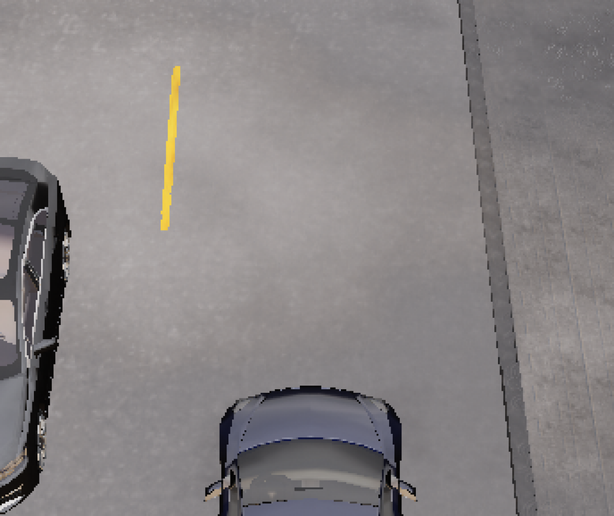
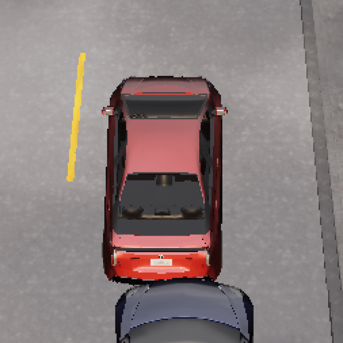
(a) Unattacked. Ego sees lane is clear and plans straight path.

(b) FP attack ATT.1. Ego emergency brakes to avoid fake obj.

(c) Unattacked. Ego stops ahead of existing stopped car.

(d) Rev-replay attack ATT.4. Ego crashes into stopped car.

Figure 4: Cyber attacks ATT.1 and ATT.4 are successful against the industry-grade Apollo driving software. Our attacks run in a docker container and intercept datagrams with the socket library as they travel from sensing to computing substrates. (top) simulation view, (bottom) camera-LiDAR fusion perception, tracking. Results against fusion suggest Apollo places large amount of confidence on LiDAR results rather than camera results for 3D perception. See Appendix D.1 for more details.

8.2 KITTI & nuScenes Datasets

We use longitudinal scenes from the KITTI and nuScenes datasets to test attack effectiveness on data captured from the real world. Prior works have explored the vulnerability of LiDAR-only perception and primitive camera-LiDAR fusion on naive and frustum attacks [49, 19]. Therefore, our case studies focus on purely novel contributions in understanding defense performance. The results are summarized below before exploring the outcomes in detail.

1. Reverse replay ATT.4 against data asymmetry 6.1 architecture. Data asymmetry may fail because camera still partially consistent with reversed LiDAR.

2. Reverse replay ATT.4 against T2T-3DLM 6.2 design. T2T-3DLM will succeed because object’s 3D position will be changed in LiDAR.

3. Frustum translation ATT.7 against data asymmetry 6.1 architecture. Data asymmetry may fail because camera will be consistent with frustum LiDAR attack.

4. Frustum translation ATT.7 against T2T-3DLM 6.2. T2T-3DLM will succeed because object’s 3D position will be changed in LiDAR.

8.3 Cases I and II: Reverse Replay ATT.4

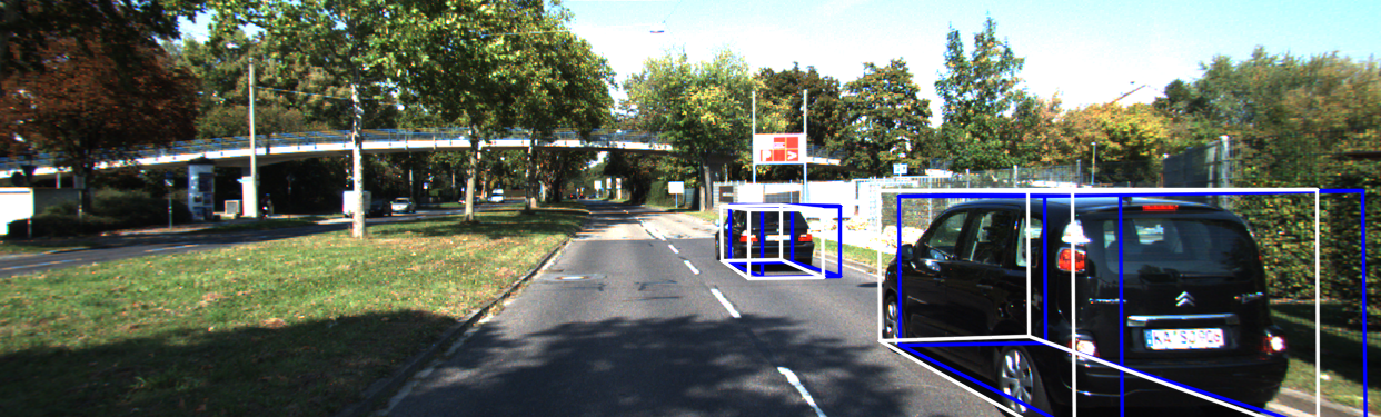
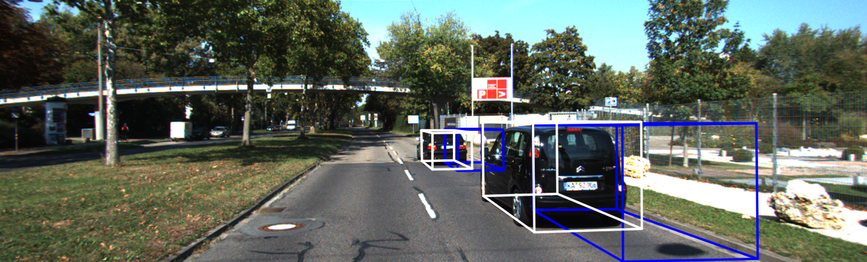
Figure 21: Front-view images of the reverse replay attack on 6.1; companion images with Fig. 5. Compare to T2T-LM3D under same attack in Fig. 22.

The attacker exploits the ambiguity of the 3D resolution of the 2D detections from the camera data. (S)He does so even without any situational awareness and only attacking LiDAR. As AVs generally move on straight or low-curvature paths, by replaying the data in reverse, it is highly likely that the 2D projection of the reverse path of an object has a high degree of overlap with the 2D projection of the continued forward path. Results are shown in Figs. 5, 6, with visualizations in Figs. 21 and 22.

8.3.1 Case I: Camera-LiDAR Fusion with 6.1.

In Fig. 5, the attacker creates FTs and MTs without altering the camera data and without any knowledge. The attack leverages the high likelihood that 2D detections from camera will be assigned as consistent with 3D detections from the reversed LiDAR. The attacker can make no guarantee of creating a safety-critical incident; the attacker is executing the reverse replay attack without any external trigger or situational awareness. To increase the likelihood of safety-critical impact, the attacker could use a lightweight monitoring algorithm to initiate the attack under favorable circumstances such as an intersection.

(a) Frame 39 (BEV)

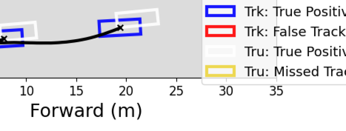
(b) Frame 46 (BEV)

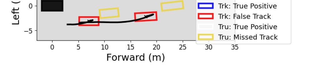
(c) Frame 51 (BEV)

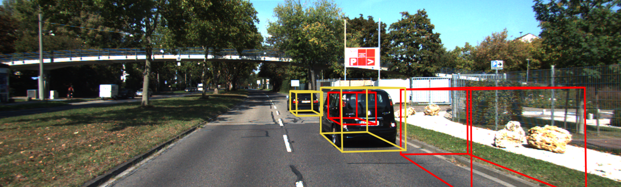
(d) Left: Frame 51 of the rev. replay attack with object tracks overlaid in camera image.

Figure 5: 6.1 design is susceptible to reverse replay ATT.4 with both FTs and MTs. Limited-capability attacker needs no estimate of any scene-specific information. Yet, no safety-critical incident occurs because object was changing lanes.

8.3.2 Case II: T2T-3DLM design 6.2.

Under a reverse replay attack, T2T-3DLM reduces incidence of FTs by identifying inconsistent information between camera and LiDAR data. Effectively, the monocular 3D detection capitalizes on image context to build a 3D track from the camera data, improving the data association in sensor fusion. Since the association is now in 3D instead of 2D, the frustum ambiguity(i.e., [19]) is no longer present. An adversary could cause two sensors to disagree (dis.) on an object while only attacking one sensor by: (dis. a) adding a fake object into one sensor, or (dis. b) removing evidence of a true object from one sensor. Currently neither 6.1’s data-asymmetry monitor nor T2T-3DLM (6.2) can distinguish between these two cases. We choose to treat both of these cases as a “fake object” and remove them (i.e., we assume (dis. a)). Unfortunately, this means both AVs are vulnerable to increased numbers of MTs if the attack is in fact (dis. b), as in Fig. 6; the replay attack has caused both a false track (T2T-3DLM can recognize this) and a missed track (T2T-3DLM cannot recognize this). In future works, a promising defense against MTs would be to use a statistical method to specifically detect a replay attack. Note that a “saturation attack” can easily be detected because it will invalidate all objects in the scene.

(a) Frame 39 (BEV)

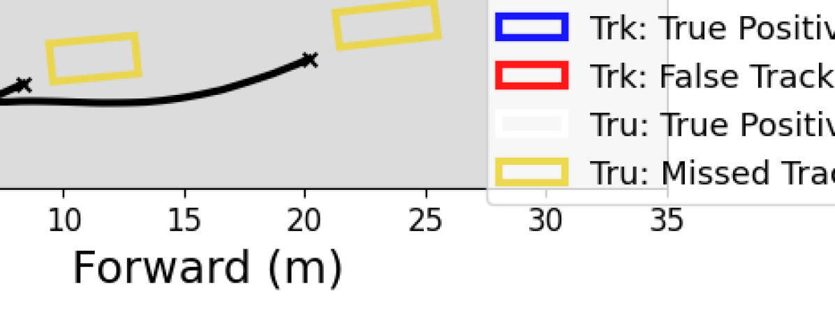
(b) Frame 52 (BEV)

Figure 6: T2T-LM3D 6.2 mitigates FTs (from Fig. 5) under a reverse replay attack ATT.4. MTs still occur.

8.4 Cases III, IV: Frust. Translation ATT.7

A frustum translation attack can have more safety consequences than a reverse replay attack. The reverse replay attack manipulates vehicles/LiDAR data in their reverse direction of travel. By contrast, a frustum-type attack manipulates vehicles/LiDAR data along the line of sight to the victim. As a result, the attacker can more easily create the appearance of a head-on collision or the illusion of a safe scene in the presence of an imminent collision.

8.4.1 Case III: Camera-LiDAR Fusion with 6.1.

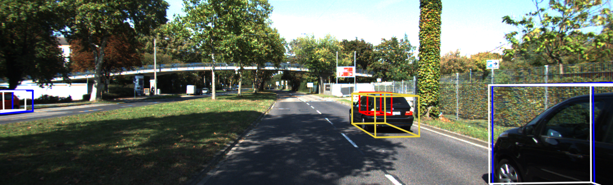
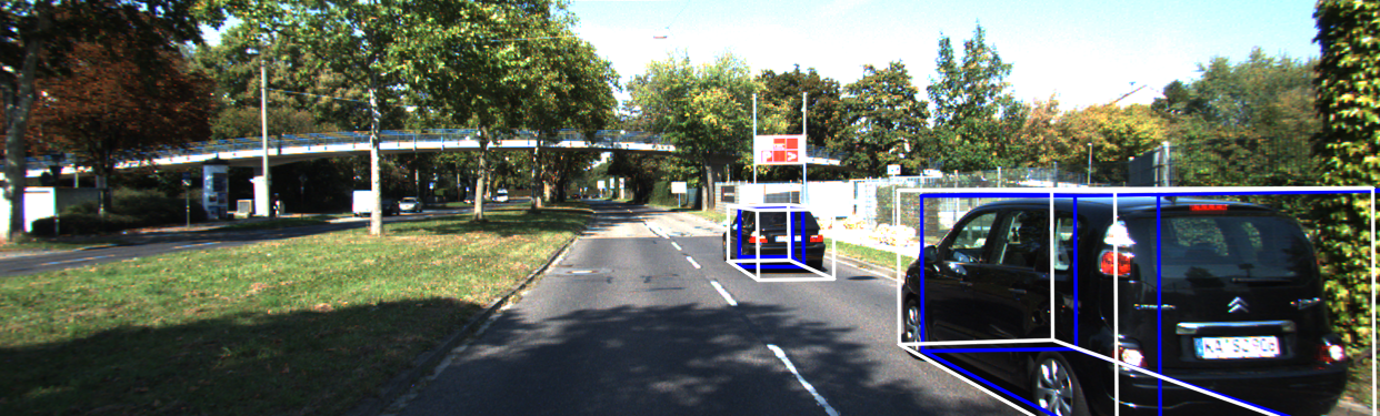
Figure 23: Front-view images of the frustum translation attack on 6.1; companion images with Fig. 7. Compare to T2T-LM3D under same attack in Fig. 24.

The consequences of a frustum translation attack are shown in Fig. 7 (additional visuals in Fig. 23). The attack leverages the frustum consistency of the camera’s 2D detections, as first presented in [19], to overtake the track of an existing object. This attack succeeds even when using 6.1 with the data-asymmetry monitor. This attack is a simultaneous FP of the inserted object and an FN of the original object, i.e., a translation outcome [19]. This new track appears to move directly toward the victim which deems this scenario unsafe using the RSS safety metric [45]. The victim must perform an evasive maneuver, even though that “unsafe” object is fictitious.

(a) Frame 29 (BEV)

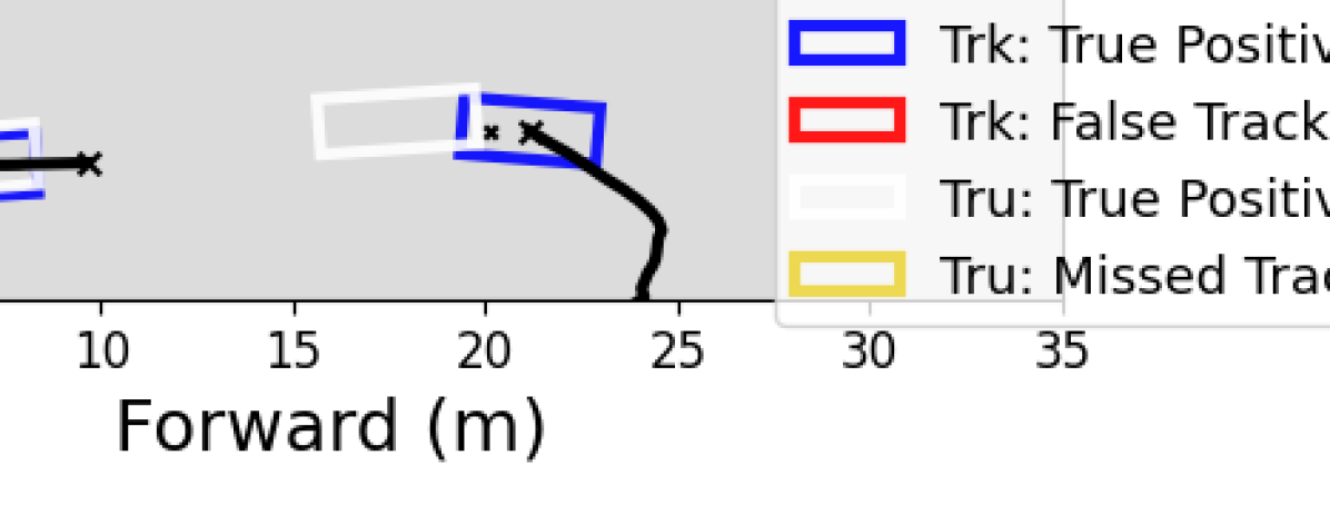
(b) Frame 38 (BEV)

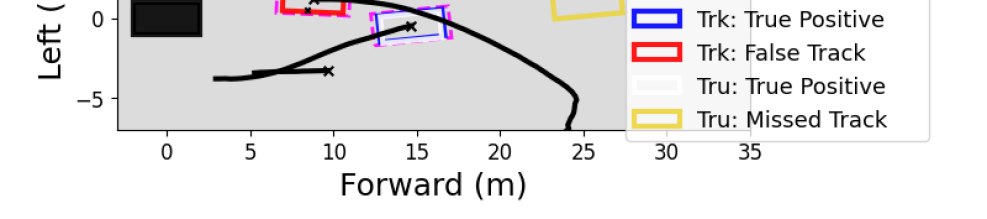
(c) Frame 61 (BEV)

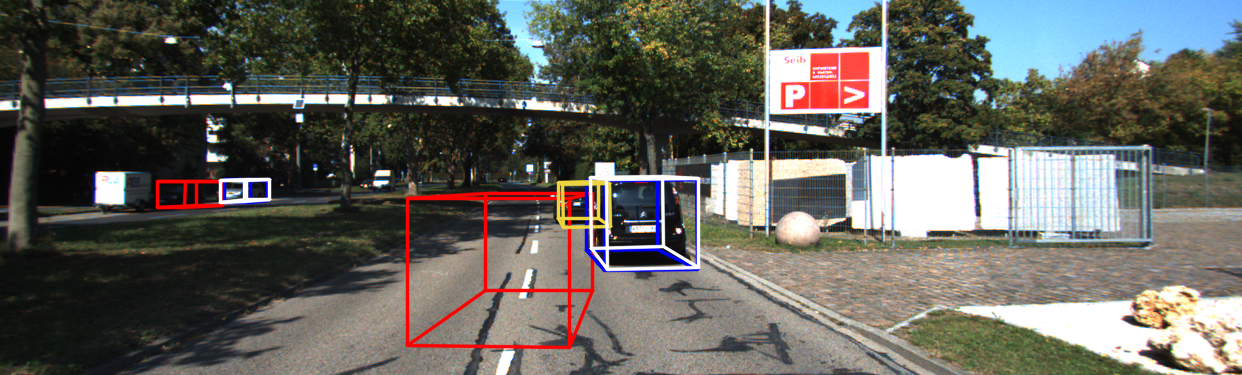
(d) Left: Frame 61 of the frust. translation attack with object tracks overlaid in camera image.

Figure 7: 6.1 is vulnerable to frustum translation attacks ATT.7 with FT and MT outcomes. Attacker monitors objects with local perception, picks a target, and translates LiDAR points to create an unsafe scene.

8.4.2 Case IV: T2T-3DLM Design  6.2.

T2T-3DLM can mitigate frustum translation attacks by fusing 3D LiDAR with monocular 3D from the camera data. This yields a more precise data association than with the 2D camera detections. In Fig. 8 (and 24), no false object is tracked by T2T-3DLM, although MT still occurs (similar to using 6.1, and similar to Case II), as T2T-3DLM once again cannot distinguish between (dis. a) and (dis. b) and assumes (dis. a). A promising defense against MTs would be to use nearby data to check for local consistency and identify translation attacks.

(a) Frame 34 (BEV)

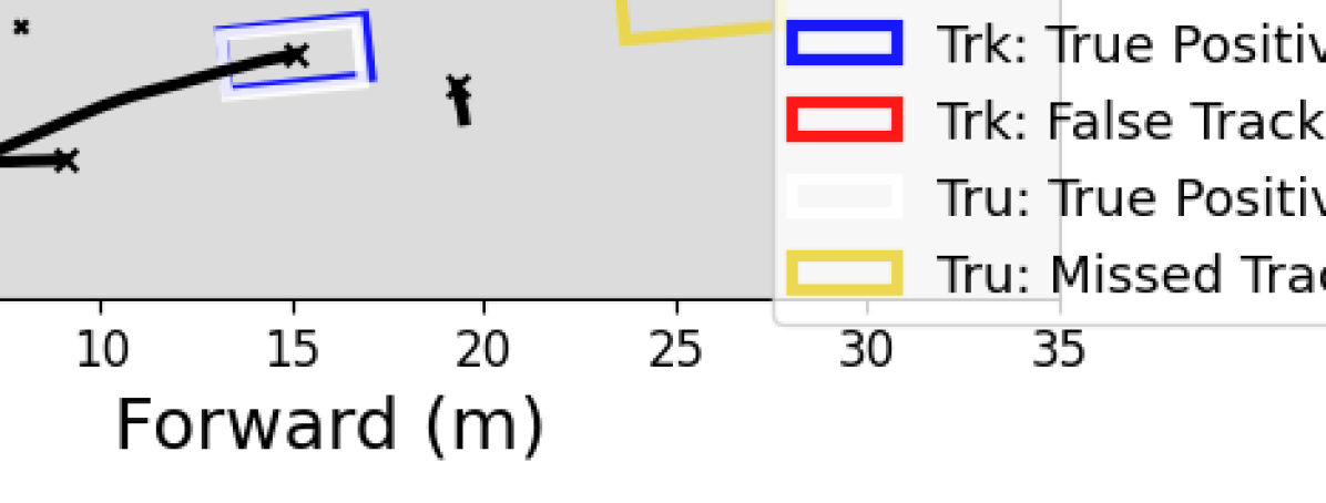
(b) Frame 62 (BEV)

Figure 8: T2T-LM3D 6.2 mitigates incidence of FTs (from Fig. 7) when experiencing a frustum translation attack ATT.7. MTs still occur, but with NO falsely-identified unsafe objects.

9 Large-Scale Evaluations

We also perform a large-scale evaluation of all attacks against all AV designs from Table III. These evaluations build a broad understanding of performance under both unattacked and attacked scenarios. From this extensive evaluation, we draw data-based insights on the merits of secure architectures in sensor fusion and the implications of our findings. Due to space constraints, here we focus on results from the reverse replay (ATT.4) and the frustum translation (ATT.7) attacks. Results for all five attacks from Sec. 4 on all validation scenes and all AV cases are presented in Table IV in Appendix E.

TABLE III: AV Configurations

Num.	AV Case Name	LiDAR	Camera	Tracking	Fusion
5	Lidar-Only	PtPillars	N/A	AB3DMOT	N/A
5	Cam-LiDAR Fusion at Detection	PtPillars	FstrRCNN	EagerMOT	N/A
6.1	Cam-LiDAR Fusion at Detection w/ Asym. Check	PtPillars	FstrRCNN	EagerMOT	N/A
6.2	Cam-LiDAR Fusion at Tracking	PtPillars	PGD	AB3DMOT (each)	T2T

Methods: For each datasets (KITTI, nuScenes), we loop over all scenes from the validation set (36 for KITTI, 135 for nuScenes). For each scene, we run each of the AV designs over the unattacked scene and capture metrics at the perception, tracking, motion prediction, and safety levels. Then, we run each of the AV designs through each of the five attacks from Sec. 4 on every scene. We capture metrics as in the unattacked baseline. Finally, we compare the baseline and attacked scenarios to isolate the effects of the attack at each module.

9.1 Baseline AV Performance

We characterize the performance of four proposed AV architectures under an unattacked baseline. In these nominal cases, the AVs are expected to have high performance and mitigate unsafe scenarios. The results of the baseline experiments are in Fig. 19 and 20 in Appendix C.1. T2T-3DLM is on par with FP performance compared to other AVs but it sacrifices a degree of MT performance at the tracking level. The results that follow present the per-frame increment over baseline – the average amount of change from the baseline to the attack case in a given metric on a per-frame basis.

9.2 Attack Effectiveness

9.2.1 Perception Outcomes

Since the LiDAR perception algorithm is constant across considered AV designs, the impact of an attack on each AV case is constant at the perception-level. Therefore, we marginalize over the AV case and show perception outcomes for each attack in Fig. 9. Attacks have intuitive outcomes at the perception level. Moving left to right in Fig. 9,

1. False positive att. ATT.1: solely FP outcomes.

2. Forward replay attack ATT.3: FP and FN identically.

3. Reverse replay ATT.4: FP and FN identically.

4. Object removal attack ATT.6: solely FN outcomes.

5. Frustum translation ATT.7: similar FP, FN outcomes.

The security-aware architectures build defense at tracking; attacks will have “success” at the perception-level alone.

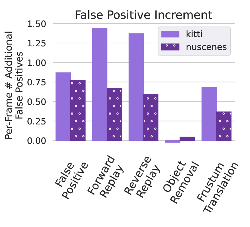
(a) FP inc. for all but removal.

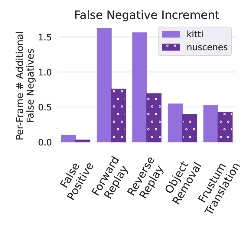
(b) FN inc. for all but false pos.

Figure 9: Perception increments over baseline (Fig. 19) per-frame marginalized over AV cases (shared LiDAR-based perception) are intuitive from attack goals.

9.2.2 Tracking Outcomes

We only discuss attacks ATT.4 and ATT.7. Table IV in Appendix E summarizes results for all attacks.

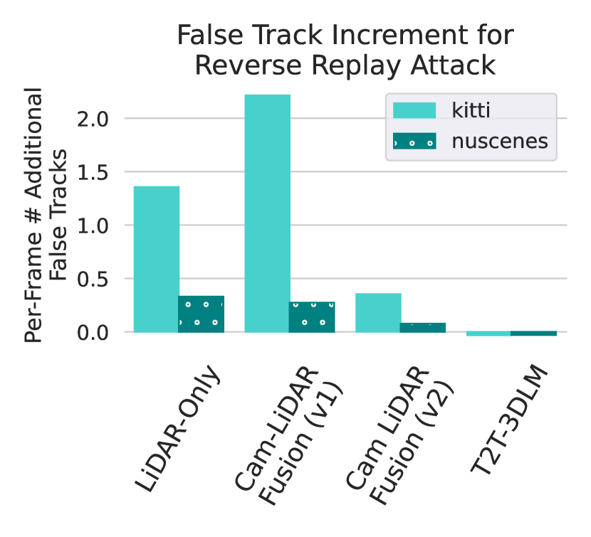
(a) (3,4) reduce per-frame FTs

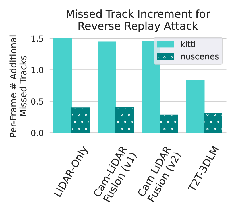
(b) All cases see MT increment.

Figure 10: Reverse replay attack: Centralized fusion with asymmetry and T2T-3DLM (cases 3, 4) mitigates FT inc. over Fig. 20. T2T-3DLM has best MT performance.

Reverse Replay Attack ATT.4. Replaying a scene has consistent temporal dynamics on straight/low-curvature paths. Thus, a replay attack will have success against both LiDAR-only and camera-LiDAR, detection-level fusion (Fig. 10). In the latter, the reverse aspect of the attack means that objects maintain consistency with their 2D bounding box detections even though only LiDAR data is manipulated; this reduces discontinuities induced by replay. Against traditional camera-LiDAR fusion, Fig. 10(a) shows reverse replay attacks induce many false and missed tracks. On the other hand, both the data asymmetry monitor and T2T-3DLM mitigate attack success with a 5-fold reduction of false tracks.

Frustum Translation Attack ATT.7. This attack is context-aware and capitalizes on both existing object tracks and camera resolution ambiguity. The attack largely increases FT and MT rates on LiDAR-only and camera-LiDAR, detection-level fusion (Fig. 11) because an existing object is targeted in the LiDAR data. The attack sees nearly a 60% success rate against camera-LiDAR fusion whereas the context-unaware false positive attack sees only 40% success (Fig. 25) in the same environment. T2T-3DLM was designed to remove the vulnerability of the ambiguity of the camera data discovered in [19]. Thus, fusion can filter out false objects inconsistent between the camera and LiDAR. The FT increment is reduced to nearly 1.0%. There is a future need to mitigate an increase in baseline missed tracks for T2T-3DLM.

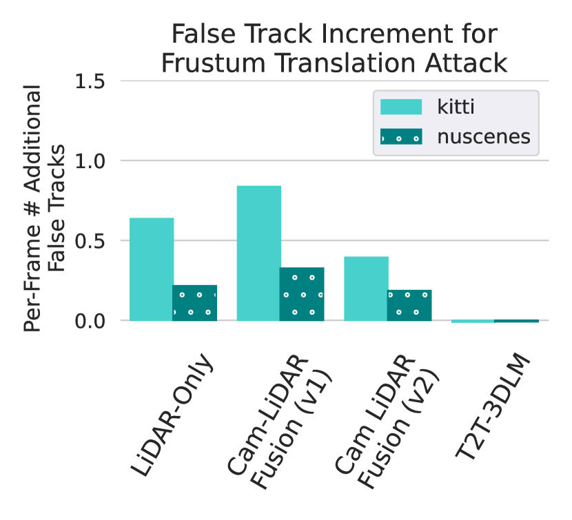
(a) (4) reduces per-frame FT

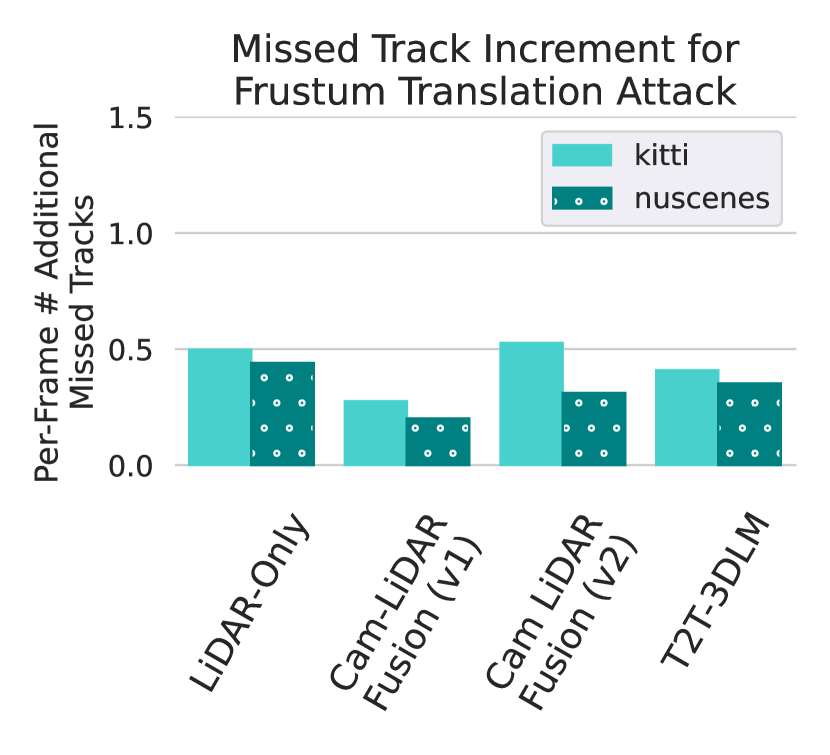
(b) All cases see MT increment.

Figure 11: Frustum translation attack: (a) Only T2T-3DLM mitigates per-frame FT increment over baseline from Fig. 20. (b) All cases have MT increment.

9.2.3 Safety Outcomes

To evaluate safety under limited-information cyber attacks on LiDAR, we use the RSS metric and three criteria for assessing safety-critical impact (Sec. 7). Changes to safety are defined as scenes where, in at least one frame, the number of unsafe objects changed from the baseline to the attacked case. Fig. 12(a) shows that the reverse replay attack induces unsafe scenarios into the first three AV designs. The attacks cause FTs to approach the victim AV and paths are restricted to existing object paths in reverse. Against traditional camera-LiDAR fusion (5), the reverse replay attack is highly successful. With no prior information or context awareness: it succeeds in generating safety-critical incidents in nearly 50% of cases. Instead, T2T-3DLM relies on estimating the full 3D object positioning from context in the camera data to obtain improved association performance and reduce attack success to 10% on average.

Fig. 12(b) shows that the frustum translation attack ATT.7 can induce many unsafe scenarios. The increase in unsafe frames for this attack is because it attacks along the line-of-sight to the victim whereas reverse replay ATT.4 only attacks along existing object paths. In both attacks, T2T-3DLM strongly mitigates the unsafe outcomes by reducing the FT presence compared to other AVs (Figs. 10(a), 11(a)). The unsafe frame increment is reduced to nearly 1.0%.

(a) Unsafe scenes in all AVs.

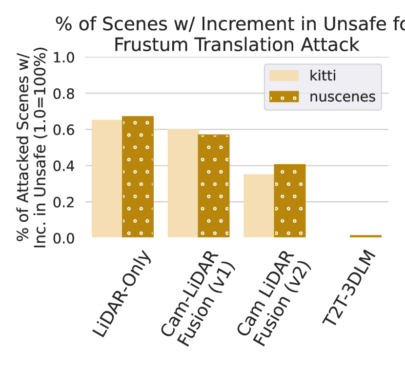
(b) (4) reduces unsafe scenes.

Figure 12: Safety evaluated via $\%$ of scenes where more frames are unsafe (measured with RSS [45]) in attack vs. baseline. T2T-3DLM mitigates strongest attack.

10 Conclusion and Discussion

We evaluated security outcomes of multi-sensor AVs with cyber attacks on LiDAR data. We considered a realistic cyber threat model with nearly no prior information about the AV or the environment. Despite these limitations, we designed eight context-unaware/aware attacks on LiDAR data and evaluated five on longitudinal datasets and AV simulators. Attacks had wide success on AV datasets, and we found even the industry-grade Baidu Apollo could be compromised by context-unaware attacks. To defend against the observed vulnerabilities, we introduced two security-aware sensor fusion designs: a data asymmetry monitor and track-to-track fusion. These approaches significantly reduced attack effectiveness in objective evaluations.

Merit of secure architectures. We demonstrated that a limited-information adversary can launch attacks by modifying LiDAR data in a purely-cyber context with only access to raw LiDAR data. We observed that the secure architectures bring many objective improvements to the AV sensing landscape. Of course, the increase in baseline missed track rate may be of concern. However, more work can be done to improve perception and tracking performance in the secure architectures without sacrificing security. Improvements in T2T-3DLM are warranted in the 3D camera-based perception algorithm and in the track identification/labeling algorithm.

Attacking other sensors. We considered LiDAR attacks due to recently discovered vulnerabilities [49, 19]. Our analyses are easily extensible to scenarios with attacking other sensors. The threat model must be updated to target the sensor(s)-of-interest; yet, the same analytical framework can be used.

10.0.1 Limitations.

For context-aware attacks, the attacker runs the SECOND [56] perception algorithm, a ‘lightweight’ LiDAR-based DNN. However, running a DNN as malware may be infeasible if the malware does not have parallel hardware. Yet, in Appendix A.1.5, the attacker does not need to use state-of-the-art perception as she can launch attacks only when detection has “high” confidence. Also, while the attacker could adaptively set scheduling parameters, we fixed the attacker’s top-level and scheduling parameters between all runs with minimal tuning. With tuning step before deploying the attack and with adaptive tuning at runtime, the attack effectiveness could be improved.

Appendix A Supplemental Attack/Defense Information

A.1 Module Partitioning

In Section 4.3, we discussed the partitioning of attacker functions into three separable modules: Monitoring, Schedule, and Execution. Algorithm 1 shows the interfaces between the partitioned modules. The partitioning is a notational and software convenience that allows for clearer description of attack implementations.

Algorithm 1 LiDAR-level attacker specified in the module-based framework. Attacker may not need to monitor “obj_tracks” for some attacks (only for some “context-aware” attacks). T_L2G is the transformation from LiDAR sensor to ground plane.

0:  LiDAR datagram $D_{k}$, frame index $k\geq 0$, obj_tracks

0:  Compromised LiDAR datagram $D_{k}^{a}$, obj_tracks

1:  T_L2G,  obj_tracks $\leftarrow$ MONITOR($D_{k}$, obj_tracks, k)

2:  if T_L2G is not NULL then

3:     attack_sched $\leftarrow$ SCHEDULE(T_L2G, tracked_objects,  k)

4:     if attack_sched is not NULL then

5:        $D_{k}^{a}$ $\leftarrow$ EXECUTE($D_{k}$,  attack_sched)

6:     end if

7:  end if

8:  return  $D_{k}^{a}$, obj_tracks

A.1.1 Monitoring

A.1.2 Sensor Height Monitoring

Fig. 13 illustrates that a simple geometric approach to estimate sensor height from the incoming data has low error against the true sensor height. Specifically, the attacker can assume that many of the lowest-elevation-angle fires will return from the ground plane. Then, the elevation angle ($\phi$) and the range on the return of that angle ($\rho$) can be used to obtain the sensor height $(h)$ as $h=\rho\sin{\phi}$. The error in sensor height estimation is minimal, as presented in the Appendix in Fig. 13. When applied to both KITTI and nuScenes datasets, this method of monitoring results in errors that do not negatively affect the attack’s performance.

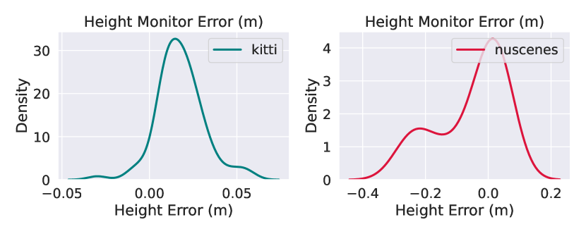
Figure 13: Attacker can use simple geometry on the point cloud or datagrams to estimate the sensor height: the height error distribution on KITII (left) and nuScenes (right) datasets. Estimate has low error on average and can be computed quickly without prior information.

A.1.3 Scheduling

A.1.4 Kinematics Models

Under this model, objects will be accelerating at an increasing rate, causing the appearance of imminent danger for the victim; the kinematic parameters evolve as:

$$j \coloneqq 6\frac{\rho_{n}-\rho_{0}}{\Delta T_{\text{attack}}^{3}},\ \quad a_{k}=a_{k-1}+j\Delta t$$ (1)

$$v_{k} =v_{k-1}+\frac{a_{k}+a_{k-1}}{2}\Delta t+\frac{1}{2}j\Delta t^{2}$$

$$r_{k} =r_{k-1}+\frac{v_{k}+v_{k-1}}{2}\Delta t+\frac{1}{2}\frac{a_{k}+a_{k-1}}{2}\Delta t^{2}+\frac{1}{6}j\Delta t^{3},$$

where $\rho_{0}$, $\rho_{n}$ are the attacker’s choice of initial and final ranges of the false object (i.e., where to start and where to end), $\Delta t$ is the time between frames, $\Delta T_{\text{attack}}$ is the overall elapsed time for the entire attack, $k$ is the index of the current frame during the attacking portion, and $j,\,a_{k}\,v_{k}\,r_{k}$ are the jerk, acceleration, velocity, and range for the false object at any time.

A.1.5 Target Object Selection

Target selection enables our attacker to see through the ‘noise’ (i.e., errors) of its perception algorithm. Unlike safety-critical AVs, the attacker only needs to find a favorable condition for attack. Context-aware attacks may target a particular object in the scene. From tracking, a set of features on each object is acquired. To construct a single per-object score, features are min-max or mean-max scaled and passed through a sigmoid function. Features are multiplied together to get the final score. The object with the lowest score is selected. If no such object exists, the attacker will wait and recompute scores at the next frame. The attack commences when a suitable object has been selected. Once a target is selected, if the attacker ever loses track of the target object, she uses the last estimated location and predicts the location to the attack time.

• Object lifetime: Objects must meet a minimum lifetime requirement of 4 frames. This mitigates attacker selecting a nonexistent (i.e., due to a false positive) “object” to target.

• Angular offset from forward: Objects must be between $[-15^{\circ},\,15^{\circ}]$ off of the forward direction of the victim. An object in a front position will have more safety-critical impact than an object from the side.

• Range to victim: Objects must be within a range of $[5\,\text{m},\,40\,\text{m}]$ from the victim. Objects in this sweet spot are more likely to become safety-relevant.

• Lateral velocity: Objects must have lateral velocities within $[-1,1]$ m/s relative to the victim. This prevents targeting objects moving in perpendicular lanes (e.g., at intersection). This is crucial for attack success.

• Forward velocity: Objects have forward velocities within $[-2,5]$ m/s relative to the victim. This prevents targeting objects in opposite lanes that will soon exit.

We test the target object selection on longitudinal cases with noisy perception algorithms. The goal is for the attacker to see through the noise of its perception – i.e., for her target selection to be robust to certain levels of its perception false positive/false negative errors), allowing her to select an appropriate object to target in the attacks. In our experiments, the attacker achieves a $57\%$ true positive rate at the perception level; almost as many false positives as true positives. These perception outcomes are very noisy; however, the attacker’s objective is not to obtain perfect perception (i.e., object detection). Instead, she can wait for the right moment, where the target can be selected with high-confidence by using tracking and scoring targets with relevant features. We find that, by adding these two components, the attacker’s target selection algorithm achieves $95\%$ in selecting a true object to target, as illustrated in Fig. 14(b).

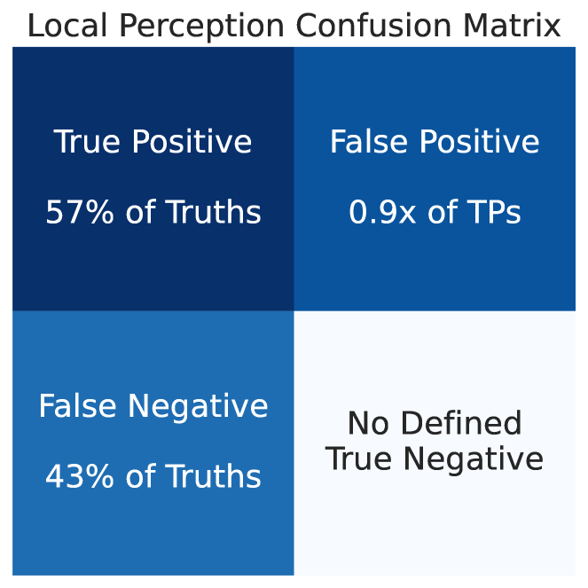
(a) Attacker only has access to one sensor (LiDAR) for building scene knowledge, leading to noisier situational awareness.

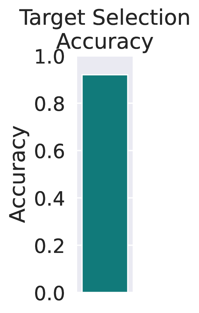
(b) Despite noisy object detection, tracking and scoring lead to accurate target selection.

Figure 14: The attacker only has access to a single sensor (LiDAR) and must run lightweight perception based on computational constraints. (a) This leads to noisy outcome of perception for the attacker; however, the attacker is not interested in obtaining perfect object detection. (b) The attacker is only interested in waiting for the “right” moment to attack. Using tracking and scoring targets by relevant features, the attacker has success ensuring targeted objects (e.g., for object removal, frustum translation) are real objects and not a false positive.

A.2 Attack Visualizations

We include visualizations of select attack procedures to aid the reader. Fig. 15 shows a step-by-step decision process that the attacker under goes for several of the attacks. For example, in the frustum translation attack, the attacker starts by monitoring existing objects in the scene. Once the attacker finds an attractive object to target, (s)he will determine where to translate that object (e.g., move towards victim). Finally, the attacker will determine which LiDAR points will encompass this new object location and will alter the range of those selected points to take the shape of an adversarial object.

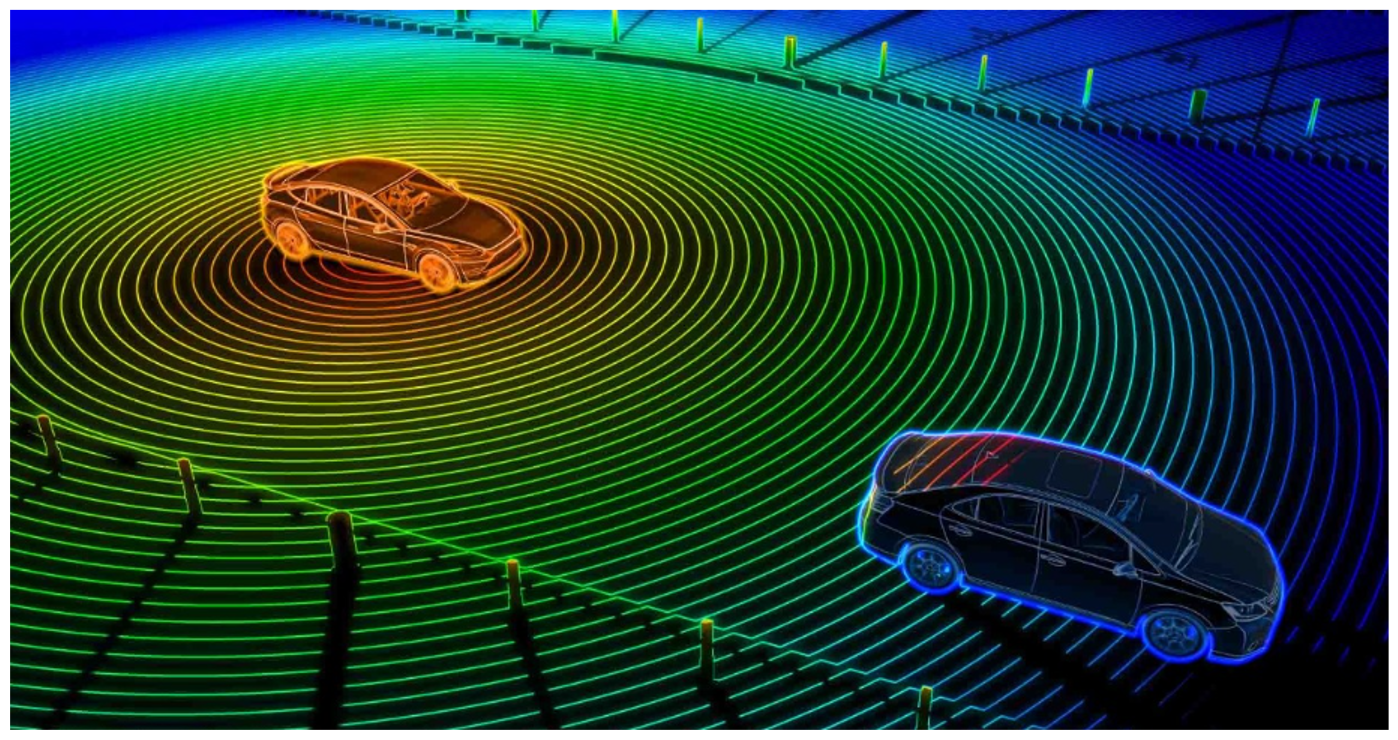
(a) True scene with victim at left (orange) and another object at right (blue). LiDAR sensor generates point cloud capture of scene which includes points reflecting from objects.

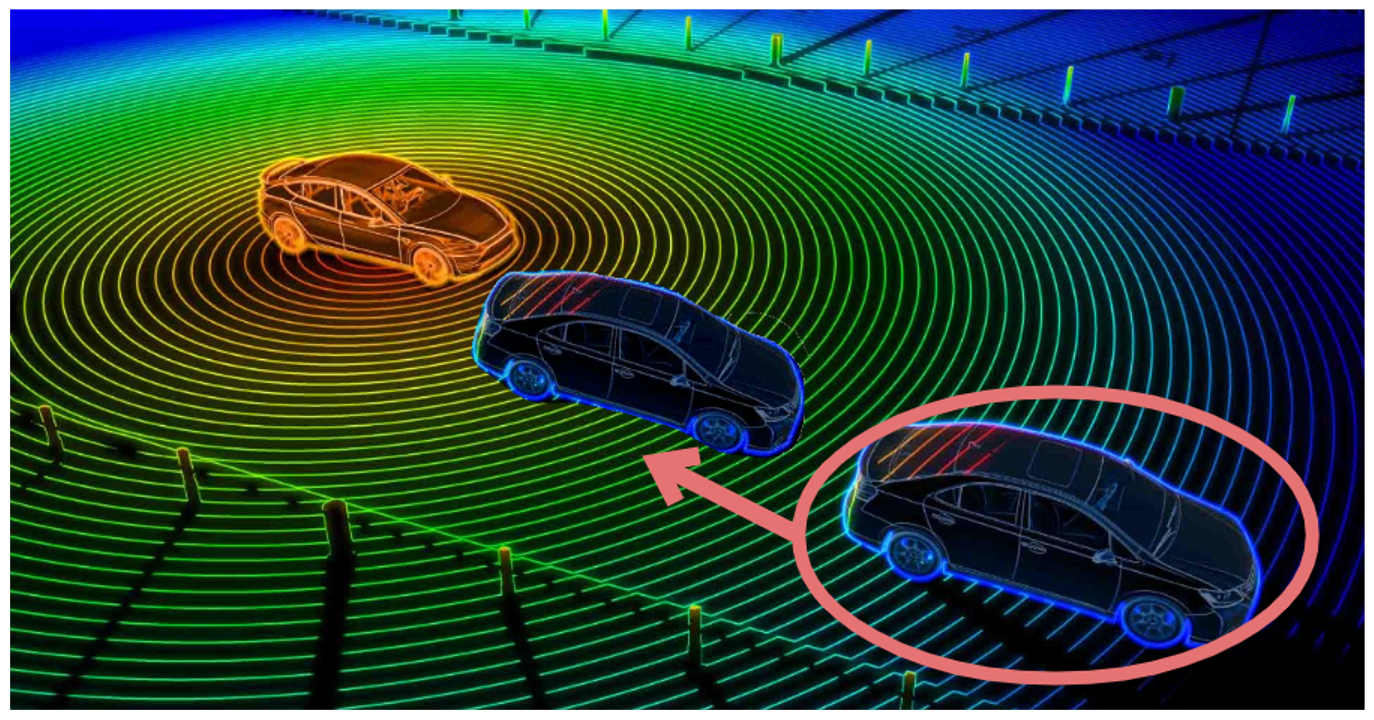
(b) Adversary manipulates other object’s points to move them closer to victim following a frustum-translation attack. Only the LiDAR points are manipulated. This can cause a false object to be detected.

Figure 15: An attacker issuing a frustum translation attack will (a) first find and select an existing object in the scene to attack. (b) Then, the attacker will manipulate the LiDAR points belonging to that object to make it appear closer or farther than the original object. The attack must only scale the range of the points, so that object will then appear to be translated directly toward or away from the victim. Base LiDAR scene image from [12].

Appendix B LiDAR Data Structures and Protocols

B.1 Notation

We use $PC$ to represent the point cloud: a set of four-dimensional points (e.g., in Cartesian coordinates, $(X,\,Y,\,Z,\,\text{intensity})$) from a full rotation of the LiDAR sensor – note that the size of $PC$ may change with each rotation, and they are stored as a matrix $[N\ \times\ 4]$ where $N$ varies over time (i.e., rotations); $D_{k}$ as a datagram (i.e., partial set of points) at time $t_{k}$; $P_{(i,j,k)}$ as one point in spherical coordinates consisting of the tuple $(\rho_{(i,j,k)},\theta_{i},\phi_{j},t_{k},I_{(i,j,k)})$ of range, azimuth, elevation, timestamp, and intensity, respectively. The set of all azimuth and elevation angles are $\{\theta_{i}\ |\ i=0,1,\dots,n\}$ and $\{\phi_{j}\ |\ j=0,1,\dots,m\}$, respectively. Visualize that the cross-product of these angles forms a matrix (i.e., columns are azimuth, rows are elevation), and the entry of each cell is a (range, intensity) pair. The cardinality measure $|\cdot|$ returns the number of items in a set.

B.2 LiDAR Data

The LiDAR sensor is composed of $m$ collinear lasers distributed vertically; see Fig. 16. Each laser provides a “vertical channel”: an elevation angle in spherical coordinates. The sensor rotates around the vertical axis. At discrete intervals, the sensor will fire its lasers, nearly in unison; each time the sensor fires, it is at a new “horizontal angle”, commonly known as an azimuth angle in spherical coordinates. A short firing time (tens of $\mu s$) means that many azimuth angles ($n$ where $n>>m$) will be captured as the sensor rotates around the vertical axis. The number of azimuth angles is determined by the firing time and the sensor rotation rate. The number of elevation angles is constrained as the number of lasers.

Fig. 17 illustrates how data flows from LiDAR sensor through the communication channels and is prepared for processing (e.g., for object detection) using Velodyne drivers. The data from the LiDAR sensor are sent incrementally for processing, via datagrams over UDP. The datagrams are compact in size and will fill prior to a full sweep of the LiDAR sensor. A single datagram is typically populated with points from a small subset of azimuth angles and all elevation angles. Thus, it requires many datagrams to compose a full point cloud. In fact, for the Velodyne-HDL32E, a datagram will fill after 12 azimuths using all 32 elevations at each azimuth. At a 10 Hz rotation rate and a $46~{}\mu s$ firing time, this means there are roughly 2100 discrete azimuth angles for full $360^{\circ}$ coverage. In turn, it will require roughly 175 datagrams to represent a full sweep [51].

Datasets and simulators represent point clouds in matrix format after postprocessing at the driver-level. Data are not saved in the datagram format that the attacker would see at the LiDAR sensor or communication substrates (Appendix B provides a discussion on datagrams). To achieve a representative attack using the point cloud matrix instead of the datagrams, we only allow the attacks to modify the range of points in the matrix while maintaining the same azimuth and elevation angles (i.e., moving a point along its unit vector from the victim AV). This is exactly what the attacker must do given access to the datagrams, as described in Sec. 3.2.3.

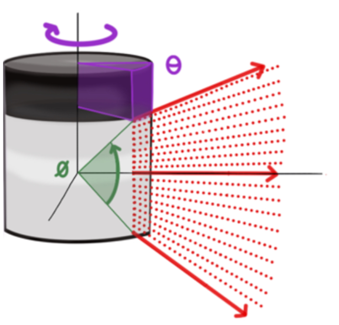
Figure 16: LiDAR sensor is composed of a single column of lasers spaced vertically. Each laser corresponds to an “elevation” angle ($\phi$). The sensor rotates about the vertical axis, and each laser will fire frequently during rotation. One full revolution provides $360^{\circ}$ “azimuth” ($\theta$) coverage.

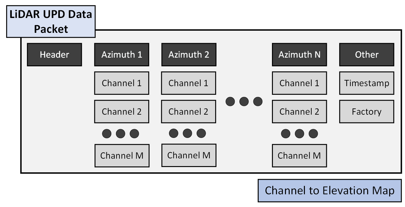
Figure 17: Datagrams take a consistent structure across all sensors within a family. For example, the VLP and HDL 16, 32, and 64 series from Velodyne take nearly identical structures (see the [51]). An attacker targeting LiDAR in a cyber-context has access to only the datagrams of LiDAR data. Similarly, the attacker is only able to manipulate the LiDAR data within the confines of the datagram structure.

B.3 First Order Data Integrity

Using the regular structure of the datagrams, a victim can implement some basic, “first-order” integrity checks on the LiDAR. These integrity checks were specified in Section 3.2.3. We formalize the integrity mathematically.

1. Max Points: The receiver knows a maximum of 1 point per angle (ppa) and 2 ppa should appear for single and dual modes, respectively. The receiver thus a-priori knows the maximum possible number of points (in the point cloud set PC) returned by the sensor. Denoting this maximum value as $\alpha$, we can introduce an integrity indicator function

   $$\zeta_{\alpha}=\left[|PC|\leq\alpha\right].$$ (2)

2. Min Points: Although it is possible for a laser to not register a return (e.g., no strong reflection), the majority of lasers will return. Hence, the receiver can a-priori set a bound on the minimum number of points (in the point cloud) returned by the sensor. Denoting this minimum value as $\beta$, the corresponding integrity indicator function is

   $$\zeta_{\beta}=\left[|PC|\geq\beta\right].$$ (3)

3. Packet Timestamps: The time interval between packets may be noisy. Assuming Gaussian noise, the difference between estimated and measured time intervals (residual) follows a $\chi^{2}$ distribution with one degree of freedom. The residual can be used as an integrity indicator function on the azimuth angle; comparing a residual normalized by expected noise, $\frac{y_{i}}{\sigma_{\gamma}}$, with a “confidence” threshold, $\gamma$, i.e.:

   $$\zeta_{\gamma}=\left[\left(\frac{y_{i}}{\sigma_{\gamma}}\right)^{2}\leq\gamma\right].$$ (4)

4. Dual Verification: If the sensor is in dual mode, the order of the returns is (strongest, last) unless the strongest is the last return in which case the order is (second strongest, last). Thus, the second return will always have larger range than the first, i.e.:

   $$\zeta_{\rho}\coloneqq\begin{cases}\texttt{False}&\texttt{mode}==\text{dual},\ \rho^{(1)}_{i,j,k}>\rho^{(2)}_{i,j,k}\\ \texttt{True}&\text{otherwise}\end{cases}$$ (5)

Finally, an aggregate receiver integrity indicator function $\zeta$ can be defined as the conjunction of all indicators; specifically,

$$\zeta\coloneqq\zeta_{\alpha}\land\zeta_{\beta}\land\zeta_{\gamma}\land\zeta_{\rho}$$ (6)

with integrity passing if $\zeta==\texttt{True}$. Basic integrity limits spoofing and mitigates nonsensical data manipulation.

Appendix C AV Implementation Details

Terminology. We borrow definitions from AVstack [20]:

• Algorithm: A specific implementation of an AV component; e.g., PointPillars [30] is an algorithm.

• Component: A generalization and grouping over algorithms; e.g., PointPillars [30] and 3DSSD [35] fall under the “3D object detection” component.

• Module: A grouping of similar components; e.g., 2D & 3D object detection $\rightarrow$ “perception” module.

• Architecture: A designed connection of components that will process data and output control signals/state.

• Implementation: A connection of algorithms that defines one particular realization of an AV architecture.

Fig. 18 presents the AV architectures from a high level. The first two follow classical LiDAR-based and centralized camera-LiDAR fusion. 5 (Fig. 18(a)) is LiDAR-based where PointPillars [30] runs on LiDAR data and resulting detections are passed to a 10-state (3-position, 3-velocity, 4-bounding-box) Kalman filter tracker, AB3DMOT [55]. 5 (Fig. 18(b)) is a centralized camera-LiDAR fusion architecture where PointPillars [30] runs on LiDAR and FasterRCNN [43] runs on camera data. Detections are then passed to the EagerMOT [28] tracker that fuses detections in a central tracker; EagerMOT is one of the few open-source methods for centralized multi-modal fusion.

The second two integrate security-aware concepts. 6.1 (Fig. 18(c)) is an extension of 5 with a data asymmetry monitor. The second, 6.2, (Fig. 18(d)) is a distributed approach to sensor fusion using concepts from distributed data fusion (DDF) [10]. This approach uses track-to-track fusion (T2T) of 3D LiDAR and monocular data (3DLM); together: “T2T-3DLM”. 3D LiDAR detections are generated from PointPillars [30] and tracked with a 10-state Kalman filter. Monocular 3D detections are also tracked with an identical 10-state Kalman filter. Tracks from each pipeline are fused by first associating with a classical assignment (e.g., JVC [25]) and then by merging assignments with covariance intersection [26].

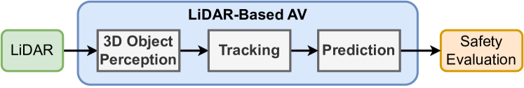
(a) LiDAR-based detection and tracking is a common single-sensor approach to AV decision.

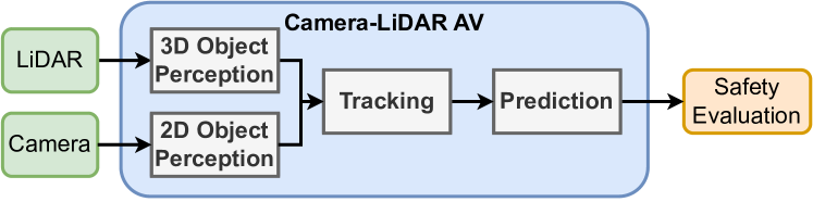
(b) Fusing data jointly at tracking can lead to improved performance over a single-modality.

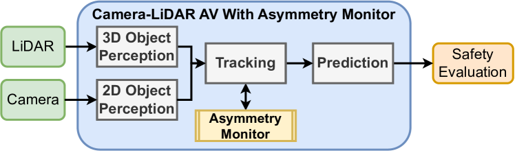
(c) Centralized fusion with data-asymmetry monitor to catch sensor mismatches.

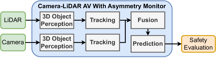
(d) T2T-3DlM: post-tracking fusion can help mitigate differences in FP/FN rates between sensor modalities.

Figure 18: Fusing information from multiple sensors can be achieved using many different architectures/designs; thus, it is critical to evaluate several common implementations.

C.1 Analysis of Baseline AV Performance

We evaluate baseline (i.e., without attacks) AV performance of the AV designs by focusing on perception and tracking outcomes in scenarios when no attacks are deployed.

Perception Outcomes. We measure the number of false positives (FP) and false negatives (FN) at the outcome of each LiDAR-based perception algorithm. All AV cases use the same LiDAR base algorithm; therefore, perception outcomes for all designs are uniform across the considered cases. Perception performance is constant across all AV cases because each AV uses the same LiDAR perception algorithm, as described in Appendix C (and Fig. 18); this is captured in the summarized analysis results in Fig. 19.

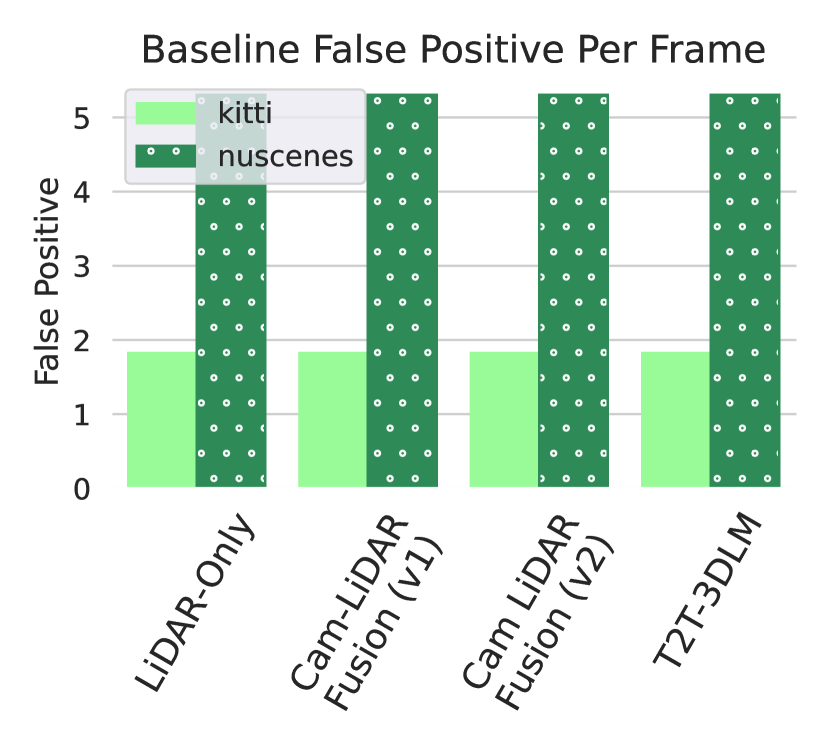
(a) Baseline FPs consistent.

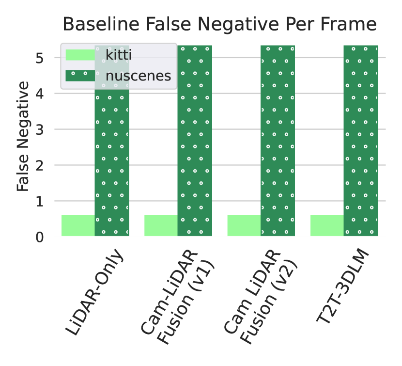
(b) Baseline FNs consistent.

Figure 19: Baseline (unattacked) AV LiDAR perception performance is constant across all AV cases because all use the same underlying LiDAR perception algorithm. nuScenes has more FP and FN than KITTI because nuScenes scenes include more complex occlusion relationships and temporal dynamics and more objects per scene.

Tracking Outcomes. The AV architectures primarily differ in sensor fusion design. We expected that without attacks, the outcomes at the tracking level will differ between AV designs. In Fig. 20, false track (FT) and missed track (MT) outcomes are reported for an unattacked baseline. As shown in Fig. 20, FT outcomes are reduced with both optimized sensor fusion (case 3) and the proposed track-to-track (T2T-LM3D) fusion (case 4). On the other hand, MT outcomes are nearly constant between cases 1, 2, and 3 in Fig. 20 with case 4 (T2T-LM3D) leading to a slight increase in MT. This trade-off between FT and MT for the T2T-LM3D approach is not surprising. In any metric that takes the form of a binary classification, an increase in false negative rate follows from a reduction in false positives. Future works will explore this trade-off beyond the binary-classification setting to determine if additional MTs of the T2T-LM3D method would lead to any safety-critical outcomes in AV simulators.

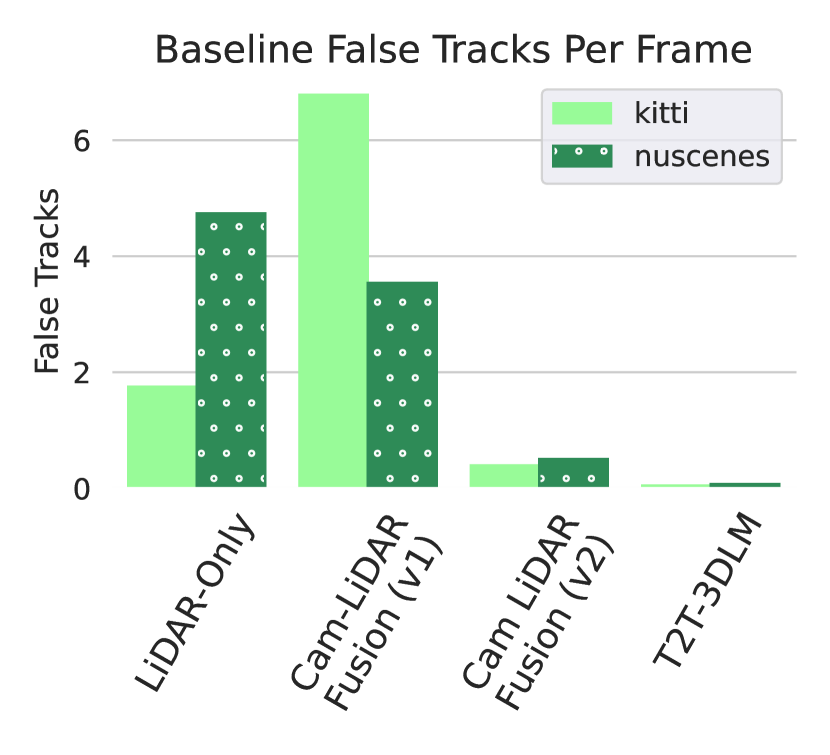
(a) Each AV arch. provides different level of FT protection.

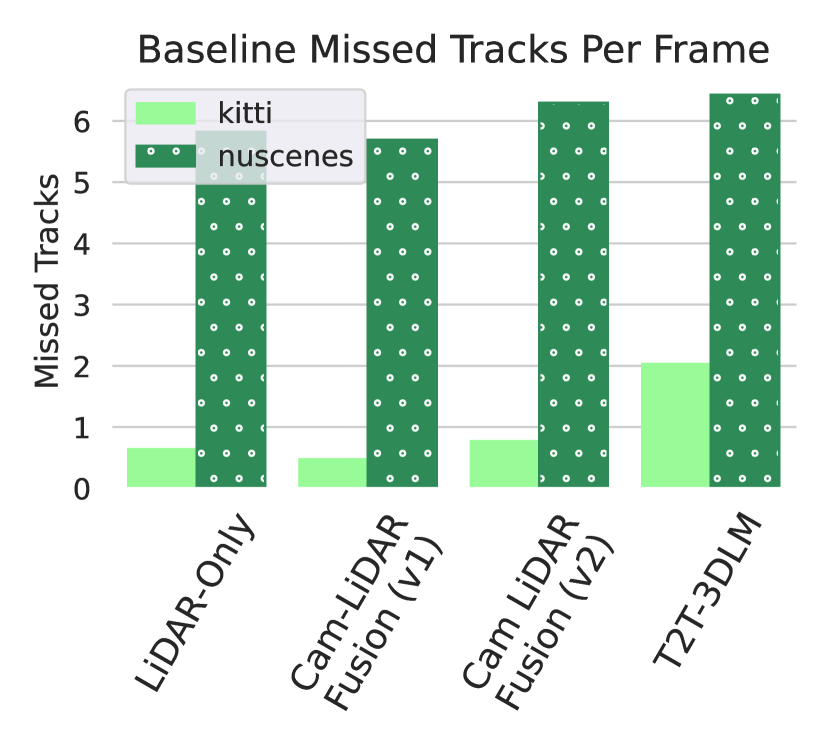
(b) MT outcomes consistent across AV arch.

Figure 20: Baseline (unattacked) AV tracking performance across 36 scenes of 150 frames in KITTI (5400 frames) and 135 scenes of 40 frames in nuScenes (5400 frames) illustrates the benefits of using sensor fusion. False tracks are mitigated with fusion and only small increase in MT observed with fusion. Fusion v1 has unacceptably high FT rate because it is not tuned appropriately. nuScenes has higher MT rate due to the much larger number of objects in scenes.

C.2 Quantifying Safety

We evaluate whether security concerns are justified in AVs by presenting evidence for safety-critical outcomes under the limited-information cyber threat model. Recent works have proposed metrics to quantify the safety of a driving situation. The Responsibility-Sensitive-Safety (RSS) [45] criteria established non-exhaustive guidelines for gauging the safety of a multi-agent situation. RSS has an open-source library and has been adopted by several prominent players in the autonomy space, including Intel’s CARLA simulator [13] and Baidu’s Apollo [3]. RSS performs a pairwise analysis of all objects in the scene. Under a “worst-case” hypothesis, RSS determines if two vehicles would crash if e.g., a front vehicle maximimally decelerated and a rear vehicle, after an average human reaction time, needed to perform an emergency maneuver to avoid the oncoming front vehicle. If the physics of the vehicles and environment allow for a safe handling of this scene, the pairwise objects are in a safe configuration. If the vehicles would crash under a worst-case scenario, they are considered to be in an unsafe configuration.

C.3 Derivation of Data Asymmetry Monitor

C.3.1 Background: Track Scoring for Confirmation

Estimation in the context of multiple target tracking combines the tasks of target existence determination and target state estimation. Namely, it is the job of the tracker to determine how many tracks are present and to estimate the states of those tracks. Regarding the task of track existence determination, a common approach is to maintain tracks on new measurements but only present tracks to downstream modules when they have been “confirmed”.

The track confirmation problem is quite settled in the literature and generally takes the form of a likelihood ratio test, as proposed by the pioneering work in [47]. Following the notation of [4], we present the likelihood ratio test for track confirmation. The likelihood ratio is:

$$\text{LR}=\frac{\Pr(D|H_{1})\Pr_{0}(H_{1})}{\Pr(D|H_{0})\Pr_{0}(H_{0})}\coloneqq\frac{P_{T}}{P_{F}}$$ (7)

where the two hypotheses, $H_{1}$ and $H_{0}$, are “track is a real target” and “track is a false alarm” hypotheses with probabilities $P_{T}$ and $P_{F}$, respectively. $D$ is the measurement data, meaning that $\Pr(D_{j}|H_{i})$ is the probability density function of the received data given that $H_{i}$ is assumed correct. Finally, $\Pr_{0}(H_{i})$ is the prior probability of the hypothesis.

When the log is taken, the likelihood ratio becomes the log-likelihood, commonly known as the “track score”

$$LLR\coloneqq L=\log\frac{P_{T}}{P_{F}}.$$ (8)

Maintaining an estimate of the track score, we can quickly revert back to the true track probability as:

$$P_{T}=\frac{e^{L}}{1+e^{L}}.$$ (9)

Conveniently, the track score can be placed in a recursive format given a simple decomposition that follows

$$L_{k} =L_{k-1}+\Delta L_{k}$$ (10)

$$\Delta L_{k} =\begin{cases}\log(1-\hat{P}_{D})\quad\text{if no update}\\ \Delta L_{k,u}\quad\text{if update.}\end{cases}$$ (11)

The “loss” (first case) component of the track score (i.e., when a track is not updated on a scan) is a function of the expected probability of detection, $\hat{P}_{D}$, of a given sensor. Intuitively, a higher probability of detection would yield a greater penalty for a missed detection ($\log$ is negative on $x\in(0,\,1)$). The “gain” (second case) component of the track score (i.e., when a track is updated on a scan) is a function of how closely the measurement matches the track state, i.e., $\Delta L_{u}$ is the likelihood of the measurement, given the track, which depends on the residual between measurement and track state. Computing this residual is a measurement-specific function.

C.3.2 Security-Awareness: Track Scoring for Validation

In traditional tracking, the data likelihood and prior probabilities consider solely information from the false alarm density model of the environment and the probability of detection model of the sensors. In other words, they do not consider the likelihood of adversarial manipulation of the inputs.

Under this traditional track confirmation logic, the adversary could easily establish a fictitious track with a high score compromising only data from a single sensor. For example, consider a two-sensor setup. If the attacker’s measurements align with the predicted dynamics model such that the residual error is small, then it is likely that the gain from the measurement likelihood ($\Delta L_{u,\text{sensor}_{1}}$) component of the track score outweighs the loss from the missed detection given the sensor’s probability of detection ($\hat{P}_{D}$). In other words, it is likely that $\Delta L_{u,\text{sensor}_{1}}>|\log\left[1-\Pr_{D,\text{sensor}_{2}}\right]|$. In the AV setting, dynamics are simple, meaning the prediction error is likely to be small. In this case, the track score will improve at every timestep even without compromising the second sensor.

As described in Section 6.1, track scoring is extended as as a defense for AV-3. In the two-sensor case, the full specification of this defense protocol is to maintain per-sensor track scores in addition to the central track score, as:

$$L_{k,\text{sensor-i}} =L_{k-1,\text{sensor-i}}+\Delta L_{k,\text{sensor-i}}$$

$$\Delta L_{k,\text{sensor-i}} =\begin{cases}\log(1-\hat{P}_{D,\text{sensor-i}})&\text{if no update}\\ \Delta L_{k,u,\text{sensor-i}}&\text{if update}\end{cases}$$

$$L_{k,\text{central}} =L_{k-1,\text{central}}+\Delta L_{k,\text{sensor}_{1}}+\Delta L_{k,\text{sensor}_{2}}.$$

Then, track confirmation is done in the usual manner where a track is confirmed when its score exceeds a designed threshold, $\tau_{c}$. Track validation is performed by monitoring the difference in track scores between pairs of sensors and triggering on a designed threshold, $\tau_{v}$ – i.e.,

Confirmation $$=\begin{cases}\texttt{Confirmed}&L_{k,\text{central}}\geq\tau_{c}\\ \texttt{Unconfirmed}&\text{otherwise}\end{cases}$$ (12)

Validation $$=\begin{cases}\texttt{Valid}&\parbox{150.00023pt}{$\texttt{Confirmed}\ \text{and}\\ |L_{k,\text{sensor}_{1}}-L_{k,\text{sensor}_{2}}|<\tau_{v}$}\\ \texttt{Invalid}&\text{otherwise}\end{cases}$$ (13)

Future Approaches. Another approach to track scoring would be to augment the traditional central track scoring with explicit sensor correspondence information in $\Delta L_{k}$. This would require deriving novel probabilistic sensor correspondence consistency metrics. This effort is left for a future work.

Appendix D Case Study Supplementals

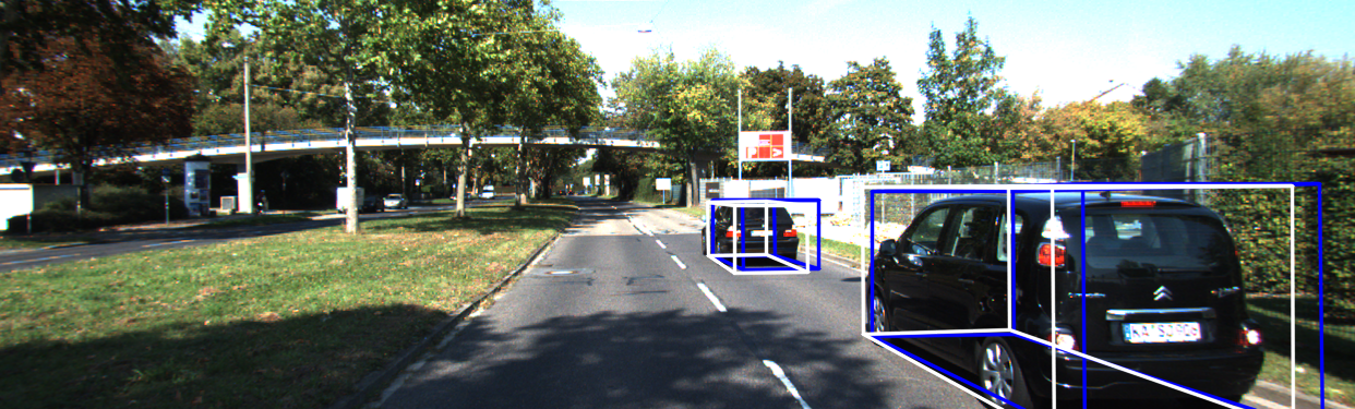
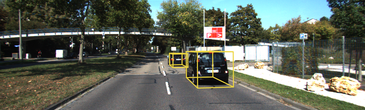
Figure 22: Front-view images of the frustum translation attack on 6.1; companion images with Fig. 6. Compare to camera-lidar detection-level fusion under same attack in Fig. 21.

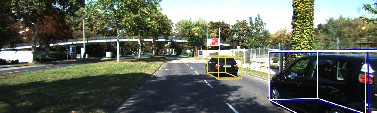
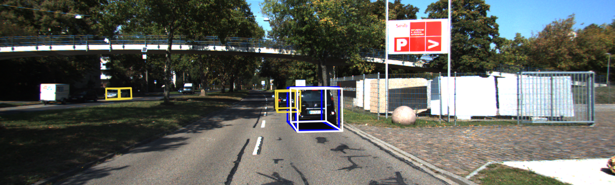
Figure 24: Front-view images of the frustum translation attack on 6.2; companion images with Fig. 8. Compare to camera-lidar detection-level fusion under same attack in Fig. 23.

D.1 Apollo Results

Apollo key: red plane with stop sign on object $\rightarrow$ object appears stopped, on ego $\rightarrow$ ego plans to (emergency) stop; green lane painting $\rightarrow$ ego plans path via lane.

Appendix E All Results

Due to space limitations, Section 9.2 provided a detailed look at attack outcomes for both KITTI and nuScenes datasets against only the reverse replay and frustum translation attacks. Here, we present results from all attacks outline in Sec. 4.

Fig. 25 and Table IV present the same information on the changes due to attack in FT, MT, and safety outcomes. Table IV also includes changes in perception outcomes that were summarized in Fig. 9.

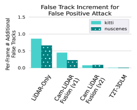
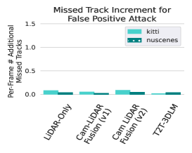
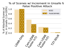
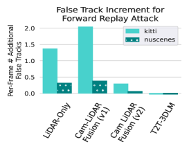
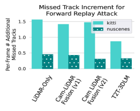
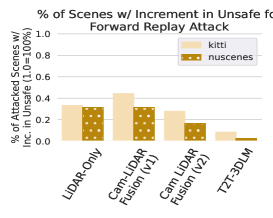
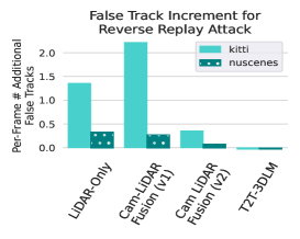
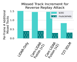
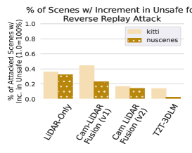
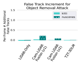
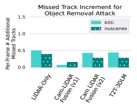
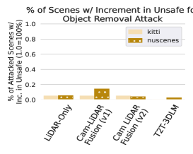
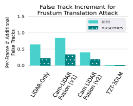
Figure 25: Column (1): Average per-frame change in the number of false tracks (“FT increment”) during the attack compared to baseline run. Column (2): Average per-frame change in the number of missed tracks (“MT increment”) during the attack compared to baseline run. Column (3): Fraction of scenes with more safety-critical incidents under attack compared to baseline.

TABLE IV: “Increment-over-baseline”, per-frame outcomes over 36 KITTI scenes of 150 frames and 135 nuScences scences of 40 frames. Red draws attention to poor performance; green to acceptable performance; blank to questionable (in-between) performance. We ignore nuScenes MT number because it is high across the board. **Safety is only tested on: “AV perceives scene unsafe, reality is safe”; important to test safety on “AV perceives scene safe, reality is unsafe” in AV simulators (see Sec. 7). e.g., all object removal attacks are deemed “safe” because an object removal attack can only induce the latter condition, not the former (tested).

AV Attacker Percep. Outcomes Track Outcomes Safety Outcomes 5 Lidar-Only ATT.1 False Positive K – FP: 0.87, FN: 0.10 N – FP: 0.77, FN: 0.03 K – FT: 0.86, MT: 0.08 N – FT: 0.66, MT: 0.03 K – Unsafe: 0.97 N – Unsafe: 1.00 5 Cam-LiDAR Fusion at Detection (v1) ATT.1 False Positive K – FP: 0.87, FN: 0.09 N – FP: 0.77, FN: 0.03 K – FT: 0.44, MT: 0.05 N – FT: 0.22, MT: 0.02 K – Unsafe: 0.56 N – Unsafe: 0.36 6.1 Cam-LiDAR Fusion at Detection (v2) ATT.1 False Positive K – FP: 0.87, FN: 0.10 N – FP: 0.77, FN: 0.03 K – FT: 0.07, MT: 0.09 N – FT: 0.08, MT: 0.05 K – Unsafe: 0.25 N – Unsafe: 0.22 6.2 Cam-LiDAR Fusion at Tracking ATT.1 False Positive K – FP: 0.87, FN: 0.09 N – FP: 0.77, FN: 0.03 K – FT: -0.00, MT: 0.01 N – FT: -0.00, MT: 0.04 K – Unsafe: 0.03 N – Unsafe: 0.02 5 Lidar-Only ATT.3 Forward Replay K – FP: 1.44, FN: 1.62 N – FP: 0.67, FN: 0.75 K – FT: 1.37, MT: 1.56 N – FT: 0.31, MT: 0.45 K – Unsafe: 0.33 N – Unsafe: 0.31 5 Cam-LiDAR Fusion at Detection (v1) ATT.3 Forward Replay K – FP: 1.44, FN: 1.62 N – FP: 0.67, FN: 0.75 K – FT: 2.04, MT: 1.41 N – FT: 0.38, MT: 0.43 K – Unsafe: 0.44 N – Unsafe: 0.31 6.1 Cam-LiDAR Fusion at Detection (v2) ATT.3 Forward Replay K – FP: 1.44, FN: 1.62 N – FP: 0.67, FN: 0.75 K – FT: 0.29, MT: 1.47 N – FT: 0.05, MT: 0.30 K – Unsafe: 0.28 N – Unsafe: 0.17 6.2 Cam-LiDAR Fusion at Tracking ATT.3 Forward Replay K – FP: 1.44, FN: 1.62 N – FP: 0.67, FN: 0.75 K – FT: -0.03, MT: 0.86 N – FT: -0.03, MT: 0.32 K – Unsafe: 0.08 N – Unsafe: 0.02 5 Lidar-Only ATT.4 Reverse Replay K – FP: 1.37, FN: 1.56 N – FP: 0.59, FN: 0.69 K – FT: 1.36, MT: 1.51 N – FT: 0.33, MT: 0.40 K – Unsafe: 0.36 N – Unsafe: 0.32 5 Cam-LiDAR Fusion at Detection (v1) ATT.4 Reverse Replay K – FP: 1.37, FN: 1.56 N – FP: 0.59, FN: 0.69 K – FT: 2.22, MT: 1.45 N – FT: 0.27, MT: 0.40 K – Unsafe: 0.44 N – Unsafe: 0.23 6.1 Cam-LiDAR Fusion at Detection (v2) ATT.4 Reverse Replay K – FP: 1.37, FN: 1.56 N – FP: 0.59, FN: 0.69 K – FT: 0.35, MT: 1.46 N – FT: 0.08, MT: 0.28 K – Unsafe: 0.17 N – Unsafe: 0.14 6.2 Cam-LiDAR Fusion at Tracking ATT.4 Reverse Replay K – FP: 1.37, FN: 1.56 N – FP: 0.59, FN: 0.69 K – FT: -0.03, MT: 0.83 N – FT: -0.03, MT: 0.31 K – Unsafe: 0.14 N – Unsafe: 0.02 5 Lidar-Only ATT.6 Object Removal K – FP: -0.02, FN: 0.54 N – FP: 0.04, FN: 0.39 K – FT: -0.03, MT: 0.49 N – FT: -0.01, MT: 0.39 K – Unsafe: 0.05 N – Unsafe: 0.05 5 Cam-LiDAR Fusion at Detection (v1) ATT.6 Object Removal K – FP: -0.02, FN: 0.55 N – FP: 0.04, FN: 0.39 K – FT: 0.03, MT: 0.06 N – FT: 0.21, MT: 0.15 K – Unsafe: 0.05 N – Unsafe: 0.14 6.1 Cam-LiDAR Fusion at Detection (v2) ATT.6 Object Removal K – FP: -0.03, FN: 0.54 N – FP: 0.04, FN: 0.39 K – FT: -0.00, MT: 0.42 N – FT: 0.07, MT: 0.28 K – Unsafe: 0.05 N – Unsafe: 0.04 6.2 Cam-LiDAR Fusion at Tracking ATT.6 Object Removal K – FP: -0.02, FN: 0.55 N – FP: 0.04, FN: 0.39 K – FT: -0.01, MT: 0.43 N – FT: -0.00, MT: 0.28 K – Unsafe: 0.00 N – Unsafe: 0.03 5 Lidar-Only ATT.7 Frustum Translate K – FP: 0.68, FN: 0.52 N – FP: 0.37, FN: 0.42 K – FT: 0.64, MT: 0.50 N – FT: 0.21, MT: 0.44 K – Unsafe: 0.65 N – Unsafe: 0.67 5 Cam-LiDAR Fusion at Detection (v1) ATT.7 Frustum Translate K – FP: 0.68, FN: 0.51 N – FP: 0.37, FN: 0.42 K – FT: 0.84, MT: 0.28 N – FT: 0.33, MT: 0.20 K – Unsafe: 0.60 N – Unsafe: 0.57 6.1 Cam-LiDAR Fusion at Detection (v2) ATT.7 Frustum Translate K – FP: 0.68, FN: 0.52 N – FP: 0.37, FN: 0.42 K – FT: 0.39, MT: 0.53 N – FT: 0.18, MT: 0.31 K – Unsafe: 0.35 N – Unsafe: 0.41 6.2 Cam-LiDAR Fusion at Tracking ATT.7 Frustum Translate K – FP: 0.69, FN: 0.52 N – FP: 0.37, FN: 0.42 K – FT: -0.01, MT: 0.41 N – FT: -0.01, MT: 0.35 K – Unsafe: 0.00 N – Unsafe: 0.01

References

- [1] anonymous authors. Cyber Attack Results. https://sites.google.com/view/av-cyber-attack/, 2023.
- [2] Autoware. Autoware. https://www.autoware.org/, 2023.
- [3] Baidu. Baidu Apollo. apollo.auto, 2023.
- [4] Samuel S Blackman. Multiple-target tracking with radar applications. Dedham, 1986.
- [5] Steve Bono, Matthew Green, Adam Stubblefield, Ari Juels, Aviel D Rubin, and Michael Szydlo. Security analysis of a cryptographically-enabled rfid device. In USENIX, volume 31, pages 1–16, 2005.
- [6] Holger Caesar, Varun Bankiti, Alex H Lang, Sourabh Vora, Venice Erin Liong, Qiang Xu, Anush Krishnan, Yu Pan, Giancarlo Baldan, and Oscar Beijbom. nuscenes: A multimodal dataset for autonomous driving. In Proceedings of the IEEE/CVF CVPR, pages 11621–11631, New York, NY, 2020. IEEE.
- [7] Han Cai, Ji Lin, Yujun Lin, Zhijian Liu, Haotian Tang, Hanrui Wang, Ligeng Zhu, and Song Han. Enable deep learning on mobile devices: Methods, systems, and applications. ACM TODAES, 27(3):1–50, 2022.
- [8] Yulong Cao, Ningfei Wang, Chaowei Xiao, Dawei Yang, Jin Fang, Ruigang Yang, Qi Alfred Chen, Mingyan Liu, and Bo Li. Invisible for both camera and lidar: Security of multi-sensor fusion based perception in autonomous driving under physical-world attacks. In 2021 IEEE Symposium on Security and Privacy (SP), pages 176–194, New York, NY, 2021. IEEE, IEEE.
- [9] Yulong Cao, Chaowei Xiao, Benjamin Cyr, Yimeng Zhou, Won Park, Sara Rampazzi, Qi Alfred Chen, Kevin Fu, and Z Morley Mao. Adversarial sensor attack on lidar-based perception in autonomous driving. In Proceedings of the 2019 ACM SIGSAC conference on computer and communications security, pages 2267–2281, London, UK, 2019. ACM.
- [10] Federico Castanedo. A review of data fusion techniques. The scientific world journal, 2013, 2013.
- [11] Stephen Checkoway, Damon McCoy, Brian Kantor, Danny Anderson, Hovav Shacham, Stefan Savage, Karl Koscher, Alexei Czeskis, Franziska Roesner, and Tadayoshi Kohno. Comprehensive experimental analyses of automotive attack surfaces. In 20th USENIX (USENIX Security 11), 2011.
- [12] Denso-X. How LiDAR Is Shaping Our Lives. https://denso-x.com/stories/how-lidar-technology-is-shaping-our-lives/, 2023.
- [13] Alexey Dosovitskiy, German Ros, Felipe Codevilla, Antonio Lopez, and Vladlen Koltun. Carla: An open urban driving simulator. In Conference on robot learning, pages 1–16. PMLR, 2017.
- [14] Christof Ebert and Capers Jones. Embedded software: Facts, figures, and future. Computer, 42(4):42–52, 2009.
- [15] Mahmoud Hashem Eiza and Qiang Ni. Driving with sharks: Rethinking connected vehicles with vehicle cybersecurity. IEEE Vehicular Technology Magazine, 12(2):45–51, 2017.
- [16] Andreas Geiger, Philip Lenz, Christoph Stiller, and Raquel Urtasun. Vision meets robotics: The kitti dataset. The International Journal of Robotics Research, 32(11):1231–1237, 2013.
- [17] Andy Greenberg. Hackers Remotely Kill a Jeep on the Highway—With Me in It. https://www.wired.com/2015/07/hackers-remotely-kill-jeep-highway/, 2015.
- [18] S Grime and Hugh F Durrant-Whyte. Data fusion in decentralized sensor networks. Control engineering practice, 2(5):849–863, 1994.
- [19] R Spencer Hallyburton, Yupei Liu, Yulong Cao, Z Morley Mao, and Miroslav Pajic. Security analysis of camera-lidar fusion against black-box attacks on autonomous vehicles. In 31st USENIX (USENIX SECURITY), pages 1–18, Berkeley, CA, 2022. USENIX.
- [20] Robert Spencer Hallyburton, Shucheng Zhang, and Miroslav Pajic. Avstack: An open-source, reconfigurable platform for autonomous vehicle development. In Proceedings of the ACM/IEEE 14th International Conference on Cyber-Physical Systems (with CPS-IoT Week 2023), pages 209–220, 2023.
- [21] Yihui He, Ji Lin, Zhijian Liu, Hanrui Wang, Li-Jia Li, and Song Han. Amc: Automl for model compression and acceleration on mobile devices. In Proceedings of the European conference on computer vision (ECCV), pages 784–800, 2018.
- [22] Geoffrey Hinton, Oriol Vinyals, Jeff Dean, et al. Distilling the knowledge in a neural network. arXiv preprint arXiv:1503.02531, 2(7), 2015.
- [23] Omar Adel Ibrahim, Ahmed Mohamed Hussain, Gabriele Oligeri, and Roberto Di Pietro. Key is in the air: Hacking remote keyless entry systems. In Security and Safety Interplay of Intelligent Software Systems: ESORICS 2018 International Workshops, ISSA 2018 and CSITS 2018, Barcelona, Spain, September 6–7, 2018, Revised Selected Papers, pages 125–132. Springer, 2019.
- [24] Yunhan Jia Jia, Yantao Lu, Junjie Shen, Qi Alfred Chen, Hao Chen, Zhenyu Zhong, and Tao Wei Wei. Fooling detection alone is not enough: Adversarial attack against multiple object tracking. In International Conference on Learning Representations (ICLR’20), pages 1–15, Addis Ababa, Ethiopia, 2020. ICLR.
- [25] Roy Jonker and Ton Volgenant. Improving the hungarian assignment algorithm. Operations Research Letters, 5(4):171–175, 1986.
- [26] Simon Julier and Jeffrey K Uhlmann. General decentralized data fusion with covariance intersection. In Handbook of multisensor data fusion, pages 339–364. CRC Press, 2017.
- [27] Samy Kamkar. Drive it like you hacked it: New attacks and tools to wirelessly steal cars. Presentation at DEFCON, 23:10, 2015.
- [28] Aleksandr Kim, Aljoša Ošep, and Laura Leal-Taixé. Eagermot: 3d multi-object tracking via sensor fusion. In 2021 IEEE International Conference on Robotics and Automation (ICRA), pages 11315–11321, New York, NY, 2021. IEEE, IEEE.
- [29] Karl Koscher, Alexei Czeskis, Franziska Roesner, Shwetak Patel, Tadayoshi Kohno, Stephen Checkoway, Damon McCoy, Brian Kantor, Danny Anderson, Hovav Shacham, et al. Experimental security analysis of a modern automobile. In 2010 IEEE symposium on security and privacy, pages 447–462, New York, NY, 2010. IEEE, IEEE.
- [30] Alex H Lang, Sourabh Vora, Holger Caesar, Lubing Zhou, Jiong Yang, and Oscar Beijbom. Pointpillars: Fast encoders for object detection from point clouds. In Proceedings of the IEEE/CVF CVPR, pages 12697–12705, New York, NY, 2019.
- [31] Ji Lin, Ligeng Zhu, Wei-Ming Chen, Wei-Chen Wang, Chuang Gan, and Song Han. On-device training under 256kb memory. arXiv preprint arXiv:2206.15472, 2022.
- [32] Zechen Liu, Zizhang Wu, and Roland Tóth. Smoke: Single-stage monocular 3d object detection via keypoint estimation. In Proceedings of the IEEE/CVF CVPR, pages 996–997, 2020.
- [33] Anthony Lopez, Arnav Vaibhav Malawade, Mohammad Abdullah Al Faruque, Srivalli Boddupalli, and Sandip Ray. Security of emergent automotive systems: A tutorial introduction and perspectives on practice. IEEE Design & Test, 36(6):10–38, 2019.
- [34] Jonathon Luiten, Aljosa Osep, Patrick Dendorfer, Philip Torr, Andreas Geiger, Laura Leal-Taixé, and Bastian Leibe. Hota: A higher order metric for evaluating multi-object tracking. International journal of computer vision, 129(2):548–578, 2021.
- [35] Qianhui Luo, Huifang Ma, Li Tang, Yue Wang, and Rong Xiong. 3d-ssd: Learning hierarchical features from rgb-d images for amodal 3d object detection. Neurocomputing, 378:364–374, 2020.
- [36] Fei Miao, Miroslav Pajic, and George J Pappas. Stochastic game approach for replay attack detection. In 52nd IEEE CDC, pages 1854–1859, Florence, Italy, 2013. IEEE, IEEE.
- [37] MITRE. Cve-2016-2354.
- [38] MITRE. Cve-2016-9337.
- [39] MITRE. Cve-2019-9977.
- [40] MITRE. Cve-2023-26246.
- [41] Yilin Mo and Bruno Sinopoli. Secure control against replay attacks. In 2009 47th annual Allerton conference on communication, control, and computing (Allerton), pages 911–918, Monticello, Illinois, 2009. IEEE, IEEE.
- [42] NHTSA. Motor vehicles increasingly vulnerable to remote exploits. Internet Crime Complaint Center (IC3), 2016.
- [43] Shaoqing Ren, Kaiming He, Ross Girshick, and Jian Sun. Faster r-cnn: Towards real-time object detection with region proposal networks. NIPS, 28, 2015.
- [44] Takami Sato, Junjie Shen, Ningfei Wang, Yunhan Jia, Xue Lin, and Qi Alfred Chen. Dirty road can attack: Security of deep learning based automated lane centering under Physical-World attack. In 30th USENIX (USENIX Security 21), pages 3309–3326, Berkeley, CA, 2021. USENIX.
- [45] Shai Shalev-Shwartz, Shaked Shammah, and Amnon Shashua. On a formal model of safe and scalable self-driving cars. arXiv preprint arXiv:1708.06374, .:1–37, 2017.
- [46] Hocheol Shin, Dohyun Kim, Yujin Kwon, and Yongdae Kim. Illusion and dazzle: Adversarial optical channel exploits against lidars for automotive applications. In International Conference on Cryptographic Hardware and Embedded Systems, pages 445–467, New York, NY, 2017. Springer, Springer.
- [47] Robert W Sittler. An optimal data association problem in surveillance theory. IEEE transactions on military electronics, 8(2):125–139, 1964.
- [48] Irshad Ahmed Sumra, JAMALUL-LAIL Ab Manan, and Halabi Hasbullah. Timing attack in vehicular network. In Proceedings of the 15th WSEAS International Conference on Computers, World Scientific and Engineering Academy and Society (WSEAS), Corfu Island, Greece, pages 151–155, 2011.
- [49] Jiachen Sun, Yulong Cao, Qi Alfred Chen, and Z Morley Mao. Towards robust LiDAR-based perception in autonomous driving: General black-box adversarial sensor attack and countermeasures. In 29th USENIX (USENIX Security 20), pages 877–894, Boston, MA, 2020. USENIX.
- [50] James Tu, Mengye Ren, Sivabalan Manivasagam, Ming Liang, Bin Yang, Richard Du, Frank Cheng, and Raquel Urtasun. Physically realizable adversarial examples for lidar object detection. In Proceedings of the IEEE/CVF CVPR, pages 13716–13725, New York, NY, 2020. IEEE.
- [51] Velodyne. Velodyne User Manual. https://velodynelidar.com/wp-content/uploads/2019/12/63-9243-Rev-E-VLP-16-User-Manual.pdf, 2019.
- [52] Swati Verma, Bhawna Mallick, and Poonam Verma. Impact of gray hole attack in vanet. In 2015 1st International conference on next generation computing technologies (NGCT), pages 127–130. IEEE, 2015.
- [53] Ziwen Wan, Junjie Shen, Jalen Chuang, Xin Xia, Joshua Garcia, Jiaqi Ma, and Qi Alfred Chen. Too afraid to drive: Systematic discovery of semantic dos vulnerability in autonomous driving planning under physical-world attacks. arXiv preprint arXiv:2201.04610, .:1–28, 2022.
- [54] Tai Wang, ZHU Xinge, Jiangmiao Pang, and Dahua Lin. Probabilistic and geometric depth: Detecting objects in perspective. In Conference on Robot Learning, pages 1475–1485. PMLR, 2022.
- [55] Xinshuo Weng, Jianren Wang, David Held, and Kris Kitani. Ab3dmot: A baseline for 3d multi-object tracking and new evaluation metrics. arXiv preprint arXiv:2008.08063, 2020.
- [56] Yan Yan, Yuxing Mao, and Bo Li. Second: Sparsely embedded convolutional detection. Sensors, 18(10):3337, 2018.
- [57] Linfeng Zhang, Runpei Dong, Hung-Shuo Tai, and Kaisheng Ma. Pointdistiller: Structured knowledge distillation towards efficient and compact 3d detection. arXiv preprint arXiv:2205.11098, 2022.
- [58] Bo Zou, Pooria Choobchian, and Julie Rozenberg. Cyber resilience of autonomous mobility systems: cyber-attacks and resilience-enhancing strategies. Journal of transportation security, pages 1–19, 2021.