Demonstration-guided Deep Reinforcement Learning for Coordinated Ramp Metering and Perimeter Control in Large Scale Networks

Abstract

Effective traffic control methods have great potential in alleviating network congestion. Existing literature generally focuses on a single control approach, while few studies have explored the effectiveness of integrated and coordinated control approaches. This study considers two representative control approaches: ramp metering for freeways and perimeter control for homogeneous urban roads, and we aim to develop a deep reinforcement learning (DRL)-based coordinated control framework for large-scale networks. The main challenges are 1) there is a lack of efficient dynamic models for both freeways and urban roads; 2) the standard DRL method becomes ineffective due to the complex and non-stationary network dynamics. In view of this, we propose a novel meso-macro dynamic network model and first time develop a demonstration-guided DRL method to achieve large-scale coordinated ramp metering and perimeter control. The dynamic network model hybridizes the link and generalized bathtub models to depict the traffic dynamics of freeways and urban roads, respectively. For the DRL method, we incorporate demonstration to guide the DRL method for better convergence by introducing the concept of “teacher” and “student” models. The teacher models are traditional controllers (e.g., ALINEA, Gating), which provide control demonstrations. The student models are DRL methods, which learn from the teacher and aim to surpass the teacher’s performance. To validate the proposed framework, we conduct two case studies in a small-scale network and a real-world large-scale traffic network in Hong Kong. Numerical results show that the proposed DRL method outperforms demonstrators as well as the state-of-the-art DRL methods, and the coordinated control is more effective than just controlling ramps or perimeters by 8.7% and 22.6%, respectively. The research outcome reveals the great potential of combining traditional controllers with DRL for coordinated control in large-scale networks.

1 Introduction

With rapid urbanization and city agglomeration, traffic congestion has become one of the most significant urban challenges in recent years. Intelligent and effective control strategies are in great need to alleviate congestion issues for public agencies. Particularly, we notice that the structure of urban road networks is in nature heterogeneous, and it consists of different types of roads (e.g., freeways and local roads) that function differently for mobility and accessibility purposes. Various control and management strategies should be enacted adaptively according to different types of roads. For instance, ramp metering is a common control method for freeways by controlling the vehicles merged into freeways from ramps (Papageorgiou et al. 1991, Wang et al. 2014), and it maintains the smoothness of the mainstream traffic by preventing the capacity drop caused by upstream queues (Cassidy and Bertini 1999, Cassidy and Rudjanakanoknad 2005). In contrast, perimeter control focuses on urban roads by restricting the inflow of vehicles into congested areas (Keyvan-Ekbatani et al. 2012; 2013), where the traffic dynamics can be modeled using the Macroscopic Fundamental Diagram (MFD) (Daganzo and Geroliminis 2008, Geroliminis and Daganzo 2008). However, how to control the traffic for heterogeneous road types is still an open question (Haddad et al. 2013).

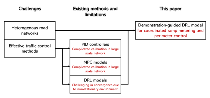
The scale of networks also limits the performance of current control methods. Previously, conventional controllers (e.g., Proportional–Integral–Derivative (PID) (Papageorgiou et al. 1991, Wang et al. 2014, Keyvan-Ekbatani et al. 2012), Model Predictive Control (MPC) (Hegyi et al. 2005, Ramezani et al. 2015), etc.) are leveraged to obtain the optimal policy on local road networks. However, these methods may require delicate calibrations in large-scale networks due to the exponentially growing problem scale and complexity. Additionally, the heterogeneity of road types on a large-scale network makes it complicated to model the network traffic dynamics (Hu et al. 2022), which also impedes the effectiveness of existing traffic control methods (Qian 2016).

In recent years, Deep Reinforcement Learning (DRL) draws attention in the research communities as it has been validated as an effective method to solve large-scale and complex control problems (Su et al. 2023, Zhou and Gayah 2023). In DRL methods, agents learn knowledge by exploring unknown environments. An agent is usually modeled with a finetuned neural network that outputs an action based on its own policy and observation. The DRL methods also demonstrate great potential in ramp metering (Fares and Gomaa 2015, Lu et al. 2017, Belletti et al. 2018) and perimeter control (Zhou and Gayah 2021; 2022), respectively. However, when the size of networks becomes large and the control scenario becomes complex, the non-stationary environment and large search spaces may also prevent the DRL from finding the optimal control policy. The non-stationary environment refers to the situation where multiple agents (i.e., ramps and perimeters) may have various control policies, and the large searching spaces are due to the size of networks.

The aforementioned challenges in the network-wide coordinated traffic control are summarized in Figure 1.

Figure 1: Challenges of existing methods for network-wide coordinated traffic control.

In this paper, we propose a novel idea to allow the DRL not only to learn by explorations from the environment but also to learn from a teacher. Conceptually, a teacher (i.e., demonstrator) can provide examples to show how to accomplish a task, and the student (i.e., our DRL agent) can use these demonstrated examples to learn knowledge through imitation and generalization. Similar ideas have been applied to games through DRL. For example, the AlphaGo algorithm (Silver et al. 2016), which learns from a combination of human expert games and self-play, can defeat the human Go champion. In the StarCraft game, the AlphaStar algorithm can reach the top human players by learning the game records (Vinyals et al. 2019). However, the idea of using demonstration guidance in engineering applications, especially in traffic control problems, has been rarely explored (Hester et al. 2017, Schmitt et al. 2018, Xiong et al. 2019). Hence this paper aims to fill the gap and develop the demonstration-guided DRL for both ramp metering and perimeter control.

For most existing demonstration-guided DRL methods, the demonstrators are human. For example, the autonomous vehicles can learn the driving behaviors from human drivers (Liu et al. 2021, Huang et al. 2022). However, it is difficult to enact a decent control policy even for a human in perimeter control and ramp metering. To this end, we adopt the traditional decentralized controllers to provide sub-optimal policies for large-scale network control, and later we will show that the student can actually outperform the teachers by integrating demonstrations and explorations.

Additionally, there is a lack of existing models that depict the traffic flow dynamics on large-scale networks with heterogeneous road types. To this end, we develop a meso-macro traffic model that integrates the mesoscopic and macroscopic dynamic traffic models for freeways and local roads, respectively. The mesoscopic link model (e.g., Asymmetric Cell Transmission Model (ACTM) (Gomes and Horowitz 2006)) depicts the flow dynamics at freeways, on-ramps, and off-ramps; and the macroscopic bathtub model manipulates vehicles in homogeneous regions (Jin 2020). Both models have been hybridized to accommodate different control scenarios in our previous studies (Hu et al. 2022), while further studies are required for DRL-based traffic control.

To summarize, this paper focuses on the coordinated ramp metering and perimeter control on large-scale networks. To model the traffic flow dynamics on heterogeneous networks, we propose a meso-macro traffic model using ACTM and generalized bathtub models. On top of that, we develop a demonstration-guided DRL method that is trained by incorporating “teacher” and “student” models. The teacher models are traditional controllers (e.g., ALINEA), which could provide imperfect control demonstrations. The student models are DRL methods, which learn from the teacher and aim to surpass the teacher’s performance. To validate the proposed framework, we conducted two case studies in a small-scale network and a real-world large-scale network in Hong Kong. The proposed method outperforms the baseline methods of existing traditional and DRL controllers in both case studies.

The major contributions of this paper are as follows:

• It formulates the coordinated ramp metering and perimeter control in a large-scale network as a DRL problem.

• It develops a novel meso-macro traffic model that supports large-scale dynamic network loading. The proposed model integrates ACTM and the generalized bathtub model for freeways and local road networks, respectively.

• It first time proposes the concept of demonstration for DRL-based traffic control, and it develops a DRL method guided by demonstrators to improve the performance of coordinated ramp metering and perimeter control.

• It conducts coordinated control experiments on both a small-scale and a real-world large-scale network in Hong Kong. The proposed method outperforms the traditional controllers and state-of-the-art DRL methods.

The rest of this paper is organized as follows. Section 2 discusses the literature related to this study. Section 3 presents the proposed framework of the dynamic traffic modeling and the DRL method. In section 4, numerical experiments at a small-scale and a real-world large-scale network in Hong Kong are presented. Finally, conclusions are drawn in section 5. All notations used in this paper are summarized in A.

2 Literature review

This section reviews the literature on related topics in this paper.

2.1 Dynamic traffic models

Based on the modeling scale and resolution, the dynamic traffic models can be categorized into the microscopic, mesoscopic, and macroscopic models (Ni 2016). Microscopic models depict vehicle acceleration and deceleration based on the interactions among vehicles nearby (Brockman et al. 2016, Wu et al. 2017, Lopez et al. 2018, Zhang et al. 2019, Bernhard et al. 2020, Zhou et al. 2020, Aimsun 2022, Liang et al. 2022, PTV Group 2022). However, due to the model complexity and traffic modeling resolution, it is nearly impossible to operate in a large-scale network. Most mesoscopic models the traffic dynamics based on vehicle queues, which simplifies the modeling of individual vehicles and increases the modeling efficiency (Milkovits et al. 2010, Zhou and Taylor 2014, Auld et al. 2016, Horni et al. 2016, Lopez et al. 2018, PTV Group 2022). However, it is still challenging to achieve a large-scale traffic modeling due to the gridlock effect (Daganzo 2007), which is a special case of the traffic congestion in which vehicles are blocked in a circular queue. The gridlock is often triggered by the improper setting of link attributes in queue-based models. The aforementioned traffic models are link-based models, and recently, the macroscopic network-based traffic models draw attention in the research community (Daganzo and Geroliminis 2008, Geroliminis and Daganzo 2008). The generalized bathtub model, a macroscopic network-based model, allows large-scale modeling, as well as decent traffic information (Jin 2020). In this paper, the macroscopic network-based model is referred to as the macroscopic model, while we omit the link-based macroscopic model as it is not suitable for dynamic traffic control. Generally, it would be beneficial to integrate the advantages of mesoscopic and macroscopic network models for large-scale networks.

2.2 Reinforcement Learning (RL) and Deep Reinforcement Learning (DRL)

RL has been extensively studied for solving Markovian decision-making problems (Sutton and Barto 2018). Traditional RL methods solve the control problem by updating a value table until convergence (Sutton 1988; 1995, Watkins and Dayan 1992). However, the complexity of such methods grows exponentially with respect to the problem complexity. With the development of Deep Learning (DL), the combination of RL and DL is a promising direction for solving high-dimensional control problems. For the discrete control, Deep Q Network (DQN) is the first DRL framework playing Atari games, which outperformed human experts. Several variants have been proposed to refine the framework (van Hasselt et al. 2016, Wang et al. 2016, Schaul et al. 2015, Bellemare et al. 2017, Fortunato et al. 2017, Hessel et al. 2018). For continuous control, Deterministic Deep Policy Gradient (DDPG) extends the DQN model with the actor-critic framework to solve the continuous control problem (Lillicrap et al. 2015). Asynchronous Advantage Actor Critic (A3C) model could accelerate the training process by incorporating distributed sampling strategy (Mnih et al. 2016). Proximal Policy Optimization (PPO) (Schulman et al. 2017) and Soft Actor-Critic (SAC) (Haarnoja et al. 2018) are advanced DRL methods for continuous control. However, in a multi-agent system, the non-stationary environment may disturb the convergence of DRL methods, resulting in poor control performance. In this study, we incorporate the demonstrated-guided DRL method to enhance the performance of coordinated ramp metering and perimeter control.

2.3 Ramp metering and perimeter control

Ramp metering serves as an important and effective freeway control strategy that has been studied in the past few decades. Previously, ramp metering can be achieved through Proportional Integral (PI) controllers (Papageorgiou et al. 1991, Wang et al. 2014, Papageorgiou et al. 1990, Papamichail et al. 2010) and MPC models (Hegyi et al. 2005). Nowadays, DRL methods gradually draw attention as they succeeded in many complex control problems. For example, Fares and Gomaa (2014) proposed an RL-based local ramp control strategy using the Q-Learning algorithm. In the follow-up work, they generalized the Q-Learning algorithm into a coordinated control with multiple ramps by integrating ramps as a centralized agent (Fares and Gomaa 2015). Centralized control of ramps can work when the ramp number is small. However, it is challenging to simultaneously control tens of ramps on the entire freeway since the space of joint action distribution will grow exponentially. To solve this problem, Belletti et al. (2018) used mutual weight regularization to reduce the impact of the high dimension of action space in multi-ramp control. Deng et al. (2019) leveraged Multi-Agent Proximal Policy Optimization (MAPPO) algorithm to improve the control performance. Lu et al. (2017) considered user equity when controlling ramps on freeways. A recent work incorporated physical-informed RL-based ramp metering using a combination of historical data and synthetic data generated from traffic models (Han et al. 2022).

Perimeter control, first proposed by Daganzo (2007), is an effective control method for urban regions. Aboudolas and Geroliminis (2013) introduced a multi-region perimeter control method using Linear Quadratic Regulator (LQR), while several studies incorporated the Proportional Integral (PI) controllers for perimeter control of urban areas (Keyvan-Ekbatani et al. 2012; 2013, Keyvan-Ekbatani, Papageorgiou and Knoop 2015, Keyvan-Ekbatani, Yildirimoglu, Geroliminis and Papageorgiou 2015). There are other methods such as MPC-based methods (Ramezani et al. 2015, Fu et al. 2017, Zhou et al. 2017, Sirmatel and Geroliminis 2018), dynamic programming (Su et al. 2020), and model-based RL methods (Chen et al. 2022) for multi-region perimeter control. Recent studies focused on data-driven and model-free adaptive control since they do not need accurate modeling of the traffic flow system, which may improve the performance in the real-world application (Lei et al. 2020, Ren et al. 2020, Li and Hou 2021, Zhou and Gayah 2023). For DRL methods, Yoon et al. (2020) proposed an RL-based for the perimeter control of a single region using the DQN model. Zhou and Gayah (2021) considered the discrete and continuous control of two regions, respectively, using Double DQN and DDPG model. They further incorporated domain control knowledge into the DRL framework to accommodate complex urban network (Zhou and Gayah 2022).

To the best of our knowledge, the topic of coordinated ramp metering and perimeter control has not been fully explored. Haddad et al. (2013) initially considered the cooperative control of two regions and a freeway using perimeter control and ramp metering. Ding et al. (2021) proposed an integral control method for the joint control of ramps and perimeters in a real-world road network. Yocum and Gayah (2022) introduced a joint control method to combine the Variable Speed Limit (VSL) and perimeter control for mixed traffic networks. In this paper, we consider the large-scale road network and focus on the joint effects of ramp metering and perimeter control.

3 Model

This section discusses the proposed framework in detail. We first present a meso-macro dynamic network model to depict the network-wide traffic dynamics, followed by the development of the demonstration-guided DRL method.

The overall framework of the coordinated ramp metering and perimeter control is shown in Figure 2. For the control problem using DRL, there are two essential modules: the environment and the agent. An environment is an object that a decision-maker will interact with to achieve a certain goal. The decision maker is viewed as an agent. The agent can observe the environment, and it can respond to the environment by taking an action based on its observations. Additionally, the agent will receive reward feedback to assess how well the action is. The agent will keep interacting with the environment to maximize its total reward. DRL concentrates on finding the optimal control policy for the agent in finite steps. For the specialized topic in this paper, an agent is either a ramp or a perimeter, the environment is the meso-macro dynamic traffic model, and the goal is to minimize Total Travel Time (TTT) for all travelers (i.e, System Optimal).

Figure 2: The framework of the coordinated ramp metering and perimeter control.

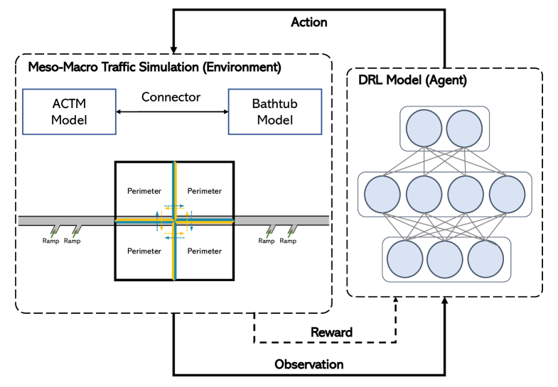
3.1 Meso-macro dynamic traffic model

The environment is depicted by the meso-macro dynamic traffic model for large-scale networks. The proposed dynamic traffic model contains two fundamental elements, the ACTM and the generalized bathtub model. The ACTM models the traffic dynamics on freeways, on-ramps, and off-ramps, and vehicles are ruled by the bathtub model in urban areas. Both models are adapted for the DRL-based traffic control. A preliminary version of this model is developed in our previous work (Hu et al. 2022), and we further extend it to model the effects of ramp metering and perimeter control.

The road network is formulated as a directed graph $\mathbf{G}=\langle\mathbf{V},\mathbf{E}\rangle$, where $\mathbf{V}$ represents the node set (i.e., merges, diverges and general junctions), and $\mathbf{E}$ represents the link set (i.e., road with different types and lanes). According to the netwrok attributes, the whole network $\mathbf{G}$ can be divided into various subgraphs $\mathbf{G}_{1},\mathbf{G}_{2},\dots,\mathbf{G}_{d},\dots,\mathbf{G}_{\mathcal{N}_{d}}\subseteq\mathbf{G}$, where $\mathbf{G}_{d}=\langle\mathbf{V}_{d},\mathbf{E}_{d}\rangle$, $\{\mathbf{V}_{1},\mathbf{V}_{2},\dots,\mathbf{V}_{d},\dots\mathbf{V}_{\mathcal{N}_{d}}\}$ is a partition of set $\mathbf{V}$. $\mathcal{N}_{d}$ means the number of partitioned regions. Each subgraph represents a region. Without loss of generality, we assume regions $\mathbf{G}_{1},\mathbf{G}_{2},\dots,\mathbf{G}_{\mathcal{N}_{d}-1}$ represent urban areas and are modeled by bathtub models; region $\mathbf{G}_{\mathcal{N}_{d}}$ presents the freeway network and is modeled by ACTM.

3.1.1 ACTM

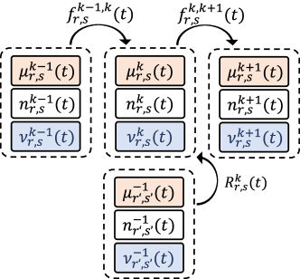
The ACTM is a generalized variant of the Cell Transmission Model (CTM) (Daganzo 1994; 1995). In the ACTM, each freeway is split into several cells which is the atomic unit of the traffic flow evolution. The difference between the ACTM and CTM is the way to model the ramps. Given a link $e_{r,s}\in\mathbf{E},r,s\in\mathbf{V}$ representing the head and tail of the link, the length of road $e_{r,s}$ is $l_{r,s}$, and the length of the cell $\delta_{r,s}$ is computed as $\delta_{r,s}=v_{r,s}^{max}\cdot\Delta t$, where $v_{r,s}^{max}$ is the free-flow speed on road $e_{r,s}$ and $\Delta t$ is the unit time interval. The illustration of the ACTM is shown in Figure 3, where $n_{r,s}^{k}(t)$ represents the vehicle number in cell $k$ on road $e_{r,s}$ at time $t$, $f_{r,s}^{k,k+1}$ is the internal traffic flow from cell $k$ to $k+1$ on road $e_{r,s}$ at time $t$, $R_{r,s}^{k}(t)$ denotes the on-ramp flow into cell $k$ on road $e_{r,s}$ at time $t$, $S_{r,s}^{k}(t)$ represents the off-ramp flow on road $e_{r,s}$ from cell $k$ at time $t$, $\mu_{r,s}(t)$ is the trip number started on road $e_{r,s}$ at time $t$, $\nu_{r,s}(t)$ is the trip number finished on road $e_{r,s}$ at time $t$, $\phi_{*,r,s}(t)$ is the external traffic flow from upstream roads into road $e_{r,s}$ at time $t$, and $\phi_{r,s,*}(t)$ is the external traffic flow from road $e_{r,s}$ to downstream roads at time $t$.

Figure 3: The illustration of the ACTM.

We name the first cell of the road $e_{r,s}$ as the “source cell” and the last cell of the road $e_{r,s}$ as the “sink cell”, respectively. In the ACTM, the conservation law of traffic flow in source cells, sink cells, general cells and on-ramp cells are formulated differently. For the conciseness of the paper, the conservation law in source cells, sink cells and general cells are discussed in B. Here, we only show the conservation law of traffic flow in on-ramp cells in Equation 1:

$$n_{r^{\prime},s^{\prime}}^{-1}(t) =n_{r^{\prime},s^{\prime}}^{-1}(t-1)+f_{r^{\prime},s^{\prime}}^{-2,-1}(t)-R_{r,s}^{k}(t),$$ (1)

$$R_{r,s}^{k}(t) =\min\left\{n_{r^{\prime},s^{\prime}}^{-1}(t-1)+f_{r^{\prime},s^{\prime}}^{-2,-1}(t),\zeta\left(\hat{n}_{r,s}-n_{r,s}^{k}(t)\right),c_{r^{\prime},s^{\prime}}(t)\right\},$$

$$c_{r^{\prime},s^{\prime}}(t) =\min\left\{q_{r^{\prime},s^{\prime}}^{max},q_{r,s}^{max}\right\},\quad e_{r,s}^{k}\text{ is not metered},$$

$$c_{r^{\prime},s^{\prime}}(t) =\rho_{r,s}^{k}(t)\min\left\{q_{r^{\prime},s^{\prime}}^{max},q_{r,s}^{max}\right\},\quad e_{r,s}^{k}\text{ is metered},$$

$$\qquad\qquad\forall r,s\in\mathbf{V},\ 2\leq k\leq\lceil l_{r,s}/\delta_{r,s}\rceil-1,$$

where $n_{r^{\prime},s^{\prime}}^{-1}(t)$ is the number of vehicles in the last cell of the road $e_{r^{\prime},s^{\prime}}$, and $e_{r^{\prime},s^{\prime}}$ is the on-ramp of $e_{r,s}$. $f_{r,s}^{-2,-1}(t)$ is the internal traffic flow from the second to last cell to the last cell (sink cell) on road $e_{r^{\prime},s^{\prime}}$ at time $t$. $\zeta$ is on-ramp flow allocation coefficient indicating the available space on the mainline for the on-ramp flow. $\hat{n}_{r,s}$ is the jam density on road $e_{r,s}$. $c_{r^{\prime},s^{\prime}}(t)$ is the inflow capacity from the on-ramp to the mainline flow. If the ramp is not metered, the inflow capacity should be equal to the minimal volume in mainline and on-ramp capacity, $q_{r^{\prime},s^{\prime}}^{max}$ and $q_{r,s}^{max}$. If the ramp is metered, the inflow capacity is determined by the metering rate $\rho_{r,s}^{k}(t)$, on-ramp, and mainline capacity. Particularly, the metering rate $\rho_{r,s}^{k}(t)$ is controllable by the DRL.

The on-ramp flow should also satisfy the following conditions:

$$R_{r,s}^{k}(t) \leq n_{r^{\prime},s^{\prime}}^{-1}(t-1)+f_{r^{\prime},s^{\prime}}^{-2,-1}(t),$$ (2)

$$R_{r,s}^{k}(t) \leq\zeta\left(\hat{n}_{r,s}(t)-n_{r,s}^{k}(t)\right),$$ (3)

$$R_{r,s}^{k}(t) \leq c_{r^{\prime},s^{\prime}}(t).$$ (4)

where Equation 2 fulfills that the on-ramp flow should not surpass the demand, Equation 3 prevents the mainstream from overload, and Equation 4 limits the on-ramp flow to the metered or non-metered capacity.

3.1.2 Generalized bathtub model

The mechanism of the bathtub model is different from that of the ACTM. In a generalized bathtub model, the movement of vehicles is no longer determined by the cell evolution but by the MFD, which models the relationship between space-mean traffic speed and regional vehicle accumulation. Hence, in a homogeneous region, all vehicles share the same speed at the same time.

Mathematically, the conservation law in a region driven by the bathtub model is formulated in Equation 5.

$$\overline{N}_{d}(t)=\overline{N}_{d}(t-1)+\overline{\mathcal{U}}_{d}(t)+\overline{\Phi}_{*,d}(t)-\overline{\mathcal{V}}_{d}(t)-\overline{\Phi}_{d,*}(t),\quad d=1,2\dots,\mathcal{N}_{d},$$ (5)

where $\overline{N}_{d}(t)$ is the vehicle accumulation in region $d$ at time $t$. $\overline{\mathcal{U}}_{d}(t)$ is the number of trips begun at region $d$ at time $t$. $\overline{\mathcal{V}}_{d}(t)$ is the number of trips finished at region $d$ at time $t$. $\overline{\Phi}_{*,d}(t)$ and $\overline{\Phi}_{d,*}(t)$ is the number of inflow and outflow of region $d$ at time $t$, respectively.

In ACTM, the evolution of the traffic flow is actuated by moving vehicles between different cells. The relative location of a vehicle on the road can be derived based on the occupied cells. In the bathtub model, such a location is difficult to track since the vehicles are on different routes with different OD pairs. To tackle this problem, the quantity of the remaining distance is utilized in the bathtub model to indicate the relative location in a region, and to guide the movement of vehicles. In the beginning, when vehicles start trips or travel from other regions, the remaining distance may not be unified. However, when they finish trips or travel to other regions, the remaining distance should be equal to zero. Supposed that $N_{d}(t,\xi)$ represents the number of vehicles in region $d$ with a remaining distance of $\xi$ and time $t$, the evolution of vehicles modeled by the bathtub model is formulated in Equation 6, 7, and 8 as follows:

$$N(t,\xi) =N(t-1,\xi+V_{d}(t)\Delta t)+\Phi_{*,d}(t,\xi)+\mathcal{U}_{d}(t,\xi),\quad\xi>0,d=1,2\dots,\mathcal{N}_{d},$$ (6)

$$N(t,0) =N(t-1,V_{d}(t)\Delta t)-\overline{\Phi}_{d,*}(t)-\overline{\mathcal{V}}_{d}(t),\quad d=1,2\dots,\mathcal{N}_{d},$$ (7)

$$V_{d}(t) =\hat{V}\left(\frac{\overline{N}_{d}(t)}{L_{d}^{sum}}\right),\quad d=1,2\dots,\mathcal{N}_{d},$$ (8)

where $V_{d}(t)$ represents the average speed in region $d$ at time $t$, $\hat{V}_{d}(\cdot)$ is the MFD of region $d$, $\Phi_{*,d}(t,\xi)$ is the vehicle inflow from upstream regions to region $d$ with the remaining distance of $\xi$ at time $t$, $\mathcal{U}_{d}(t,\xi)$ is the vehicle numbered started in region $d$ with a remaining distance of $\xi$ at time $t$, and $L_{d}^{sum}$ is the total length of roads in region $d$.

Equation 6 models the evolution of vehicles with non-zero remaining distance, where only inflow and departing vehicles will show up in the region. Equation 7 depicts the evolution of vehicles with zero remaining distance. If the remaining distance of a vehicle is zero, the vehicle will either be transferred to other regions or completes the trip. Equation 8 illustrates that the regional average speed is correlated with the average vehicle density in a region.

The derivation of the external traffic flow is presented in Equation 9 for $d=1,2\cdots,\mathcal{N}_{d}$.

$$\overline{\Phi}_{*,d}(t) =\sum_{i\in\Psi^{-}(d)}\overline{\Phi}_{i,d}(t),$$ (9)

$$\overline{\Phi}_{d,*}(t) =\sum_{j\in\Psi^{+}(d)}\overline{\Phi}_{d,j}(t),$$

$$\overline{\Phi}_{i,d}(t) =\hat{\Phi}\left(\left\{\mathfrak{D}_{j}(t)|\forall j\in\Psi^{-}(d)\right\},\left\{\mathfrak{S}_{k}(t)|\forall k\in\Psi^{+}(d)\right\}\right),$$

$$\overline{\Phi}_{d,j}(t) =\hat{\Phi}\left(\left\{\mathfrak{D}_{i}(t)|\forall i\in\Psi^{-}(j)\right\},\left\{\mathfrak{S}_{k}(t)|\forall k\in\Psi^{+}(j)\right\}\right),$$

where $\Phi_{i,d}(t)$ denotes the external traffic flow from region $i$ into region $d$. $\hat{\Phi}(\cdots)$ represents a function that allocates the external flows in different regions by transferring vehicles between regions. $\mathfrak{D}_{j}$ is the demand in region $d$ at time $t$, and $\mathfrak{S}_{d}$ is the supply in region $d$ at time $t$. $\Psi_{d}^{-}$ and $\Psi_{d}^{+}$ means sets of upstream and downstream regions that directly connect to region $d$, respectively.

Perimeter control aims to improve the network throughput by limiting the traffic inflow into congested urban areas at the boundary of regions. Hence, the quantitative value should be related to the maximal capacity at the boundary. Equation 10 shows the computation of the regional supply, demand, and boundary capacity.

$$\mathfrak{D}_{d}(t) =\min\left\{N_{d}(t,0)-\overline{\mathcal{V}}_{d}(t),C_{d,+}^{margin}\right\},$$ (10)

$$\mathfrak{S}_{d}(t) =\min\left\{\hat{N}_{d}-\overline{N}_{d}(t)-\mathcal{U}_{d}(t),C_{d,-}^{margin}\right\},$$

$$C_{d,+}^{margin} =\sum_{e_{r,s}\in E,r\in\mathbf{V}_{d},s\not\in\mathbf{V}_{d}}q_{r,s}^{max},$$

$$C_{d,-}^{margin} =\begin{cases}\sum_{e_{r,s}\in E,r\not\in\mathbf{V}_{d},s\in\mathbf{V}_{d}}q_{r,s}^{max}&\mathbf{G}_{d}\text{ is not controlled}\\ \mathcal{P}_{d}(t)\sum_{e_{r,s}\in E,r\not\in\mathbf{V}_{d},s\in\mathbf{V}_{d}}q_{r,s}^{max}&\mathbf{G}_{d}\text{ is controlled}\\ \end{cases},$$

$$\hat{N}_{d} =\sum_{e_{r,s}\in E,r,s\in\mathbf{V}_{d}}\hat{n}_{r,s},$$

where $C_{d,+}^{margin}$ is the boundary capacity for vehicle outflow while $C_{d,-}^{margin}$ is the boundary capacity for vehicle inflow, and $\mathcal{P}_{d}(t)$ is the control rate for region $d$ at time $t$. If the region $d$ is controlled, the vehicle inflow should not exceed the total road capacity at boundaries $\sum_{e_{r,s}\in E,r\not\in\mathbf{V}_{d},s\in\mathbf{V}_{d}}q_{r,s}^{max}$ with a fraction of $\mathcal{P}_{d}(t)$. Let $\hat{N}_{d}$ represent the total jam density in region $d$. Additionally, the relationship between the flow evolution and conservation law in the bathtub model is shown in Equation 11 for $d=1,2\cdots,\mathcal{N}_{d}$.

$$\overline{N}_{d}(t) =\int_{\xi=0}^{L_{d}^{max}}N(t,\xi)d\xi,$$ (11)

$$L_{d}^{sum} =\sum_{r,s\in\mathbf{V}_{d}}l_{r,s},$$

$$L_{d}^{max} \leq L_{d}^{sum},$$

where $L_{d}^{max}$ is the length of the longest route in region $d$.

3.2 Demonstration-guided DRL method

The proposed DRL method contains two modules, the decision-making module and the demonstrator. The decision-making module aims to learn an optimal control policy by exploring the environment, and the demonstrator generates demonstration data to guide the learning of the decision-making module.

3.2.1 Partially Observable Markov Decision Process

The interaction between agents and the environment can be formulated as a Partially Observable Markov Decision Processes (POMDPs), in which agents can access limited information from the environment. The POMDPs can be depicted by a 6-tuple $(\mathcal{X},\mathcal{U},\mathcal{P},\mathcal{R},\Omega,\mathcal{O})$. At each timestep $t$, a state incorporating the full environment information is $\mathbf{x}_{t}\in\mathcal{X}$. An agent can observe the environment and obtain the observation $\mathbf{o}_{t}\in\Omega$ with a probability of $\mathbf{o}\sim\mathcal{O}(x)$. The environment will evolve into a new state $\mathbf{x}_{t+1}\sim P(\mathbf{x}_{t},\mathbf{u}_{t})$ when the agent takes an action $\mathbf{u}_{t}\in\mathcal{U}$. The objective of a single agent at time $t$ is to maximize the discounted cumulative rewards it will obtain in the future before the termination of the interaction, which is formulated in Equation 12.

$$G_{t}=\sum_{\tau=t}^{\hat{T}^{term}}\lambda^{\tau-t}\mathbf{r}_{\tau},$$ (12)

where $G_{t}$ represents the discounted cumulative reward from the start time $t$, $\hat{T}^{term}$ is the termination step, and $\lambda$ is the discount factor that balances the short-term and long-term returns. The action value function $Q(\mathbf{x}_{t},\mathbf{u}_{t})$ measures the expectation of reward when an agent takes action $\mathbf{u}_{t}$ at state $\mathbf{x}_{t}$ at time $t$, which is defined in Equation 13:

$$Q_{\pi}(\mathbf{x}_{t},\mathbf{u}_{t})=\mathbb{E}\left(G_{t}|\mathbf{x}_{t},\mathbf{u}_{t}\right).$$ (13)

Specifically, in this paper, the definitions of an agent, state, observation, action, and reward are shown as follows.

Agent

An agent in the meso-macro network could be either a ramp or a perimeter. While the former type of agent controls the inflow from ramps, the latter type of agent controls the inflow into congested urban areas. Since this study models traffic control as a POMDP problem, an agent can obtain partial observations and historical information $\mathbf{o}_{t}$ and $\mathbf{h}_{t}$ rather than state information $\mathbf{x}_{t}$. The agent takes an action $\mathbf{u}_{t}$ from its own policy $\pi(\mathbf{o}_{t},\mathbf{h}_{t})$, and receives a reward $\mathbf{r}_{t}$ from the environment.

State and observation

In the road network, the state information consists of the trip source, sink, vehicle accumulation, and traffic flow in the ACTM cells and the generalized bathtub regions for all the roads and regions. However, in the real world, an agent may not receive all state information in the whole network due to the limitation of network bandwidth and information processing speed. A plausible setting would be that agents can receive local information from their neighbors (i.e., adjacent ACTM cells and bathtub regions). The local information consists of node information and edge information as follows:

• For an ACTM cell, the node information includes the trip started number (if it is a source cell), the trip completed number (if it is a sink cell), and the vehicle number in the ego cell. The edge information includes the internal traffic flow between different cells. Then for a ramp, the observation consists of local information of adjacent cells. An example of the observation of a ramp cell is shown in Figure 4(a). The adjacent cells include the upstream cell, the downstream cell, and the connected ramp cell. There are 12 variables in node information, and 3 variable in edge information. In total, the dimension of observation of a ramp agent is 15.

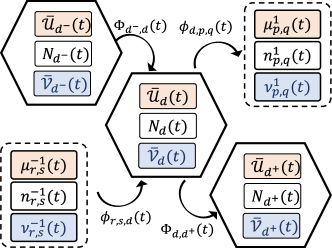
• For a bathtub region, the node information includes the trip started number, trip completed number, and the vehicle accumulation in this region, while the edge information incorporates the external traffic flow from or to different ACTM cells or bathtub regions. The observation consists of local information of adjacent cells and regions. An example of a perimeter cell is shown in Figure 4(b). The neighbors include source cells and sink cells in the ACTM, and regions in the bathtub model. Since the number of surroundings is not fixed for a perimeter agent, the dimension varies in different perimeter agents.

(a) An example of an ACTM agent.

(b) An example of a bathtub agent.

Figure 4: Two example agents of the ACTM and bathtub region.

Action

In a ramp metering task, the metering rate $\rho_{r,s}^{k}(t)$, which is a continuous scalar ranging in $[\mathbf{u}_{min},\mathbf{u}_{max}]$ in Equation 1 is set to adjust the percentage of vehicle inflow from on-ramps. In the perimeter control task, the boundary inflow rate $\mathcal{P}_{d}(t)$, which is also a continuous scalar ranging in $[\mathbf{U}_{min},\mathbf{U}_{max}]$ in Equation 10 is defined in each region to control the inflow vehicles from other regions to ease congestion. Since it is challenging to achieve a continuous coordinated control for multiple ramps and perimeters simultaneously due to the huge action space when the number of controllable agents is large, we cast the continuous action space into a discrete decision-making process. There are three options for each agent, raise the control rate by a minimal change step $\Delta\mathbf{u}$, keep the current control rate and reduce the control rate by $\Delta\mathbf{u}$. Hence the action space for each agent falls in $\mathbf{u}_{t}\in\mathbb{R}^{3}$.

Reward

The coordinated ramp metering and perimeter control framework aims to minimize the TTT of all travelers in the network. Mathematically, the minimization of the average TTT for all travelers is expressed in Equation 14, where $\mathcal{N}_{p}$ is the number of trips, and $T_{i}^{end}$ and $T_{i}^{start}$ is the end time and start time for trip $i$.

$$\min\frac{1}{\mathcal{N}_{p}}\sum_{i=0}^{\mathcal{N}_{p}}\left(T_{i}^{end}-T_{i}^{start}\right)$$ (14)

If we integrate Equation 14 along with the timeline, the minimization of the average TTT can be approximated to the maximization of the sum of vehicle completion from time $t$ to $t+\Delta t$. The derivation is shown in Equation 15.

$$\min\frac{1}{\mathcal{N}_{p}}\sum_{i=0}^{\mathcal{N}_{p}}\left(T_{i}^{end}-T_{i}^{start}\right) \approx\max\frac{\Delta t}{\mathcal{N}_{p}}\sum_{i=0}^{\lceil T^{term}/\Delta t\rceil}\left(\mathcal{N}_{inj}(i\Delta t)-\mathcal{N}_{run}(i\Delta t)\right),$$ (15)

$$=\max\frac{\Delta t}{\mathcal{N}_{p}}\sum_{i=0}^{\lceil T^{term}/\Delta t\rceil}\mathcal{N}_{com}\left(i\Delta t,(i+1)\Delta t\right),$$

$$\leftrightarrow\sum_{i=0}^{\lceil T^{term}/\Delta t\rceil}\max\mathcal{N}_{com}\left(i\Delta t,(i+1)\Delta t\right),$$

where $\mathcal{N}_{inj}(i\Delta t)$ denotes the accumulative injected vehicle at time $i\Delta t$, $\mathcal{N}_{run}(i\Delta t)$ represents the number of running vehicles at time $i\Delta t$, and $\mathcal{N}_{com}(i\Delta t,(i+1)\Delta t)$ represents the number of completed vehicles from time $i\Delta t$ to time $(i+1)\Delta t$. The optimal solution is lower bounded by $\max\sum_{i=0}^{\lceil T^{term}/\Delta t\rceil}\mathcal{N}_{com}\left(i\Delta t,(i+1)\Delta t\right)\geq\sum_{i=0}^{\lceil T^{term}/\Delta t\rceil}\max\mathcal{N}_{com}\left(i\Delta t,(i+1)\Delta t\right)$, which means that agents can greedily take actions that can maximize the vehicle completion number for now. Though it may not be the optimal solution for the minimal TTT, the network efficiency can also be improved by taking the control policy that makes most trips completed in the current time interval. Therefore, the step-wise rewards for all controllable agents are set as the number of completed trips from $t$ to $t+\Delta t$. Furthermore, we normalize the reward with a baseline constant $C_{r}$. The final reward is defined in Equation 16.

$$\mathbf{r}_{t}=\mathcal{N}_{com}(t,t+\Delta t)-C_{r}$$ (16)

3.2.2 Deep Q network

In the fully observable MDP for the model-free control problem, the action value function $Q(\mathbf{x},\mathbf{u})$ is utilized to evaluate the expectation of return after taking an action $\mathbf{u}$ at state $\mathbf{x}$ under the policy $\pi$. In simplified control problems with finite states, the $Q(\mathbf{x},\mathbf{u})$ can be derived from tabular updating methods (e.g., Q-Learning (Watkins and Dayan 1992), sarsa (Sutton 1995), etc.). The policy is taking the action with the maximal $Q$ value, which is formulated as

$$\pi\left(\mathbf{u}_{t}|\mathbf{x}_{t}\right)=\begin{cases}1,\quad\text{if }Q(\mathbf{x}_{t},\mathbf{u}_{t})=\max_{\hat{\mathbf{u}}_{t}}\left(Q\left(\mathbf{x}_{t},\hat{\mathbf{u}_{t}}\right)\right)\\ 0\end{cases}.$$ (17)

For a complex control problem, the $Q(\mathbf{x},\mathbf{u})$ is difficult to be acquired from direct tabular searching since the $Q(\mathbf{x},\mathbf{u})$ is hard to converge in a limited time with a large state and action space. To solve $Q(\mathbf{x},\mathbf{u})$ in complex control problems, the action value function approximation, which treats the $Q(\mathbf{x},\mathbf{u})$ as a function of state and action $\hat{Q}:\mathbf{x}\times\mathbf{u}\rightarrow Q\in\mathbb{R}$, is leveraged to approximate the real action value $Q(\mathbf{x},\mathbf{u})$. Two significant contributions have been made to stabilize the training process, the experience replay buffer and the target network. The replay buffer collects transition tuples of state, action, reward and next state $(\mathbf{x}_{t},\mathbf{u}_{t},\mathbf{r}_{t},\mathbf{x}_{t}^{\prime})$ for each time $t$ in a sequential manner. The DQN model can request the transition in the buffer replay at the training stage in multiple times, which enhances the sample efficiency. Furthermore, it breaks down the temporal correlation between transitions, which may enhance the final control performance. The usage of the target network leads the Q-network (source network) to converge by cloning the weights of the Q-network periodically. To optimize the Q-network weight, the loss function is defined as

$$L_{RL}=\left(\mathbf{r}_{t}+\lambda\max_{\mathbf{u}_{t+1}}Q(\mathbf{x}_{t+1},\mathbf{u}_{t+1};\theta^{-})-Q(\mathbf{x}_{t},\mathbf{u}_{t};\theta)\right)^{2},$$ (18)

where $\theta^{-}$ is the weight of the target network and $\theta$ is the weight of the Q network.

3.2.3 Demonstration-guided DQN

To enhance the performance of coordinated control of ramps and perimeters, we incorporate demonstrators to guide agents in learning control policies. There are three rules when selecting demonstrators. 1) The demonstrator should be simple to acquire; 2) The demonstrator should be efficient; 3) The performance of the demonstrator should be decent. Based on these rules, we choose ALINEA (Papageorgiou et al. 1991) as the demonstrator for the ramp agent and Gating (Keyvan-Ekbatani et al. 2012) as the demonstrator for the perimeter agent, respectively. More information regarding the demonstrators can be referred to C.

The cross entropy can be utilized to measure the discrepancy between a demonstrator policy $\overline{\pi}\left({\mathbf{u}_{t}}|\mathbf{x}_{t}\right)$, and the model policy $\pi\left({\mathbf{u}_{t}}|\mathbf{x}_{t}\right)$. In the proposed DRL method, the cross entropy is defined as:

$$L_{CE}(t)=-\sum_{\mathbf{u}_{t}\in\mathbf{U}}\pi\left({\mathbf{u}_{t}}|\mathbf{x}_{t}\right)\log\overline{\pi}\left({\mathbf{u}_{t}}|\mathbf{x}_{t}\right).$$ (19)

The DRL method approximates the action value function $\hat{Q}:\mathbf{x}\times\mathbf{u}\rightarrow Q\in\mathbb{R}$, which takes the state and action as inputs and outputs the Q value. According to Equation 17, the final action is selected as the one with the maximal Q value (i.e., $\operatorname*{argmax}_{\mathbf{u}_{t}}Q\left(\mathbf{x}_{t},\mathbf{u}_{t}\right)$). As the “argmax” operation cannot contribute gradient to the DRL method in the backpropagation, we involve a dummy policy $\tilde{\pi}\left({\mathbf{u}_{t}}|\mathbf{x}_{t}\right)$, which takes the “softmax” operation of the original Q values, shown in Equation 20.

$$\tilde{\pi}\left({\mathbf{u}_{t}}|\mathbf{x}_{t}\right)=\frac{\exp{\left(Q\left({\mathbf{u}_{t}},\mathbf{x}_{t};\theta\right)\right)}}{\sum_{\hat{\mathbf{u}}_{t}\in\mathbf{U}}\exp{\left(Q\left({\hat{\mathbf{u}}_{t}},\mathbf{x}_{t};\theta\right)\right)}}$$ (20)

The demonstration loss that distinguishes the demonstrator and the DRL method is represented in Equation 21

$$L_{D}(t)=-\sum_{\mathbf{u}_{t}\in\mathbf{U}}\tilde{\pi}\left({\mathbf{u}_{t}}|\mathbf{x}_{t}\right)\log\overline{\pi}\left({\mathbf{u}_{t}}|\mathbf{x}_{t}\right)$$ (21)

Replacing $\pi\left({\mathbf{u}_{t}}|\mathbf{x}_{t}\right)$ by $\tilde{\pi}\left({\mathbf{u}_{t}}|\mathbf{x}_{t}\right)$, we are able to calculate the gradient and conduct backpropagation to minimize the demonstration loss $L_{D}(t)$ in Equation 21. Note that $\tilde{\pi}\left({\mathbf{u}_{t}}|\mathbf{x}_{t}\right)$ does not represent the actual policy for taking actions. In contrast, it approximates the actual policy and ensures the easy derivation of gradients when training the DRL.

3.2.4 Solution framework

Since we model the coordinated control problem as a POMDP, the historical information can be utilized to compensate for the deficiency in the state information. The action value function can be modeled as a function of observation, historical information, and action $\hat{Q}:\mathbf{o}\times\mathbf{h}\times\mathbf{u}\rightarrow Q\in\mathbb{R}$. The framework of the proposed demonstration-guided DRL method is shown in Figure 5. For each agent $i$ at time $t$, it observes trip start, trip end, vehicle accumulation, and traffic flow information in neighboring roads and regions, $\mathbf{o}_{t}^{i}$. The observed information was initially encoded by the “observation encoder” module, which is a Multilayer Perceptron (MLP). The encoded information was combined with encoded historical information $\mathbf{h}_{t-1}^{i}$ in the Long short-term memory (LSTM) module which outputs the next historical information $\mathbf{h}_{t}^{i}$ and estimated action value $Q_{i}\left(\mathbf{o}_{t}^{i},\mathbf{h}_{t-1}^{i},\mathbf{u}_{t}^{i}\right)$ for all eligible actions. The output action is selected according to the $\epsilon$-greedy policy to balance the exploration of the environment and the exploitation of the model. Specifically, the action will be selected with the maximal action value, $\operatorname*{argmax}_{\mathbf{u}_{t}}Q_{i}\left(\mathbf{o}_{t}^{i},\mathbf{h}_{t-1}^{i},\mathbf{u}_{t}^{i}\right)$, with the probability of $1-\epsilon$, and will be selected randomly in the action space with the probability of $\epsilon$. Interacting with the environment, each agent $i$ will receive a reward $\mathbf{r}_{t}^{i}$ and it can observe the environment again to acquire knowledge $\mathbf{o}_{t+1}^{i}$, and the transition information includes a tuple of $\left[\mathbf{h}_{t-1},\mathbf{o}_{t},\mathbf{u}_{t},\mathbf{r}_{t},\mathbf{o}_{t+1}\right]$.

Figure 5: The framework of the proposed demonstrated guided DRL method.

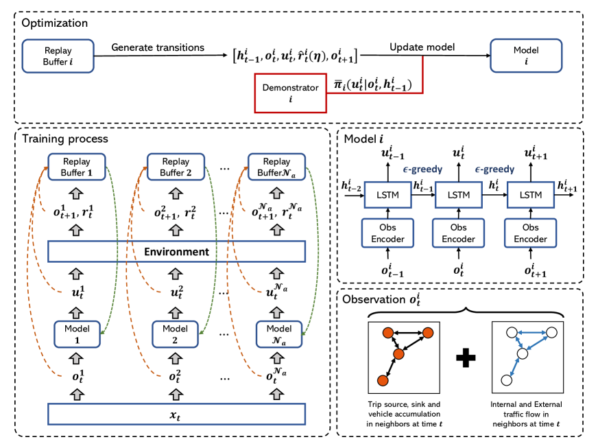
To optimize the proposed DRL method, the final loss function for each agent is formulated in Equation 22 and  23. It incorporates two parts. The first part is the traditional DQN loss modeled in POMDP. The multi-step return mechanism that exposes further information to the current state is also incorporated to fasten the convergence of the DRL method. The second part is the demonstration loss which measures the discrepancy between the demonstrator policy and the agent policy.

$$L^{i}(t)=L_{RL}^{i}(t)+\alpha_{t}L_{D}^{i}(t)$$ (22)

$$L_{RL}^{i}(t) =\left(\hat{\mathbf{r}}_{t}^{i}(\eta)+\lambda^{\eta}\max_{\mathbf{u}_{t+1}^{i}}Q_{i}\left(\mathbf{o}_{t+1}^{i},\mathbf{h}_{t}^{i},\mathbf{u}_{t+1}^{i};\theta_{i}^{-}\right)-Q_{i}\left(\mathbf{o}_{t}^{i},\mathbf{h}_{t-1}^{i},\mathbf{u}_{t}^{i};\theta_{i}\right)\right)^{2}$$ (23)

$$L_{D}(t) =-\sum_{\mathbf{u}_{t}\in\mathbf{U}}\tilde{\pi}_{i}\left({\mathbf{u}_{t}^{i}}|\mathbf{o}_{t}^{i},\mathbf{h}_{t-1}^{i}\right)\log\overline{\pi}_{i}\left({\mathbf{u}_{t}^{i}}|\mathbf{o}_{t}^{i},\mathbf{h}_{t-1}^{i}\right)$$

$$\hat{\mathbf{r}}_{t}(\eta) =\sum_{i=1}^{\eta}\lambda^{\eta}\mathbf{r}_{t+i},$$

To balance the traditional DQN loss and demonstration loss, there is also a time-varying annealing factor $\alpha_{t}$, which is defined in Equation 24. There are 4 parameters that adjust the annealing factor in each epoch: $\alpha_{min}$, $\alpha_{step}$, $\alpha_{term}$, and $\alpha_{amp}$. In the training stage, the annealing factor is a large number at the beginning, hence $L_{RL}^{i}(t)\ll\alpha_{t}L_{D}^{i}(t)$. The DRL method is constrained by the demonstrator without any exploration to resemble supervised training. Such a constraint anneals with time, and when $\alpha_{t}$ is close to $0$, $L_{RL}^{i}(t)\gg\alpha_{t}L_{D}^{i}(t)$, the training loss is close to the DQN loss, which permits the agent to learn a better policy through exploration and exploitation of the environment.

$$\mathcal{A}(t) =1-\frac{1}{1+\exp(-\alpha_{min}-\alpha_{step}*t)}$$ (24)

$$\alpha_{t} =\begin{cases}\alpha_{amp}*\frac{\mathcal{A}(t)-\mathcal{A}(\alpha_{term})}{\mathcal{A}(0)-\mathcal{A}(\alpha_{term})}&,t\leq\alpha_{term}\\ 0&,t>\alpha_{term}\end{cases}$$

The pseudo-code for learning the proposed demonstration-guided DRL method is presented in Algorithm 1.

1 for Agent $i=1,\dots,\mathcal{N}_{a}$ do

2       Randomly initialize replay buffer $B^{i}$ to capacity $\mathcal{N}_{B}$;

3       Initialize the historical information $h^{i}_{0}=\overrightarrow{0}$;

4       Initialize the Q-network with random weights $\theta_{i}$;

5       Clone the Q-network weight $\theta_{i}$ to the target network weight $\theta_{i}^{-}$ ;

6      

7 end for

8for Epoch $m=1,\dots,\mathcal{N}_{m}$ do

9       for Time Interval $t=1,\dots,T$ do

10             for Agent $i=1,\dots,\mathcal{N}_{a}$ do

11                   Select a random action $\mathbf{u}_{t}^{i}$ with probability of $\epsilon(m)$ ;

12                   Otherwise select $\mathbf{u}_{t}^{i}=\operatorname*{argmax}_{\mathbf{u}}Q\left(\mathbf{o}_{t}^{i},\mathbf{h}_{t-1}^{i},\mathbf{u}_{t}^{i};\theta_{i}\right)$ with probability of $1-\epsilon(m)$;

13                   Obtain historical information $\mathbf{h}_{t}^{i}$; 

14             end for

15            Execute actions $\left\{\mathbf{u}_{t}^{1},\mathbf{u}_{t}^{r},\dots,\mathbf{u}_{t}^{\mathcal{N}_{a}}\right\}$ in the simulator. Obtain rewards $\left\{\mathbf{r}_{t}^{1},\mathbf{r}_{t}^{2},\dots,\mathbf{u}_{t}^{\mathcal{N}_{a}}\right\}$ and observe $\left\{\mathbf{o}_{t+1}^{1},\mathbf{o}_{t+1}^{2},\dots,\mathbf{o}_{t+1}^{\mathcal{N}_{a}}\right\}$;

16             for Agent $i=1,\dots,\mathcal{N}_{a}$ do

17                   Store transition $\left[\mathbf{h}_{t-1}^{i},\mathbf{o}_{t}^{i},\mathbf{u}_{t}^{i},\mathbf{r}_{t}^{i},\mathbf{o}_{t+1}^{i}\right]$ in $B^{i}$;

18                  

19             end for

20            

21       end for

22      for Optimization Step $k=1,\dots,\mathcal{N}_{o}$ do

23             for Agent $i=1,\dots,\mathcal{N}_{a}$ do

24                   Sample random mini-batch of transitions $\left[\mathbf{h}_{j-1}^{i},\mathbf{o}_{j}^{i},\mathbf{u}_{j}^{i},\mathbf{r}_{j}^{i},\mathbf{o}_{j+1}^{i}\right]$;

25                   Update the $\theta_{i}$ by minimizing the loss in Equation 22;

26                  

27             end for

28            

29       end for

30      Update the annealing factor $\alpha_{m}$ according to Equation 24;

31       if $(m\mod\mathcal{N}_{c})==0$ then

32             for Agent $i=1,\dots,\mathcal{N}_{a}$ do

33                   Clone the Q-network weight $\theta_{i}$ to the target network weight $\theta_{i}^{-}$;

34                  

35             end for

36            

37       end if

38      

39 end for

Algorithm 1 Demonstration-guided DRL method for coordinated ramp metering and perimeter control

4 Numerical experiments

In this section, two case studies are presented to evaluate the proposed demonstration-guided DRL method for coordinated ramp metering and perimeter control. In the first case study, the effectiveness of the proposed method is tested in a small-scale network with 4 on-ramps and 4 perimeters. In the second case study, we examine the proposed framework in a real-world large-scale network in Kowloon District, Hong Kong SAR, with a real-world demand in the morning peak.

4.1 Settings of experiments

For the meso-macro network model, the unit time interval is set to one second, and agents will interact with the environment every 30 seconds. The on-ramp flow parameter, $\gamma$, is set to 1 and the on-ramp flow allocation coefficient $\zeta$ is fixed to 1. The lower bound and the upper bound of the control rate for ramps and perimeters, $\mathbf{u}_{min}$, $\mathbf{U}_{min}$, and $\mathbf{u}_{max}$, $\mathbf{U}_{max}$ are set to $0.1$ and $1$, respectively. The change step of the control rate $\Delta u$ is set to $0.05$, which means the current control rate will increase or decrease by $0.05$. Moreover, if the current control rate exceeds the upper bound or lower bound $\mathbf{u}_{min}$, $\mathbf{U}_{min}$ and $\mathbf{u}_{max}$, $\mathbf{U}_{max}$, the actual control rate will be truncated. In real world, the daily traffic demand may fluctuate, resulting in uncertainty of the congestion patterns for ramps and perimeters. To replicate the randomness of the traffic demand, given a demand profile, the actual traffic demand follows a normal distribution where the mean is the given demand for each OD pair, and the standard deviation is 30% of the demand mean.

For the DRL method, in both case studies, the number of neurons in a 3-layer MLP is 100, 100, and 3 respectively. The hyperparameters regarding the DRL method are the same except for the number of epochs. The choices of hyperparameters are listed in Table 1. The value of $\epsilon(t)$ will decay exponentially in the training stage to trade off between exploration and exploitation. The Adam optimizer is chosen in both case studies for optimizing the DRL method with the learning rate of $3e^{-6}$. The batch size for each sampling in the replay buffer is 128. The replay buffer makes use of the queue with the First In First Out (FIFO) property.

Hyperparameter	Value	Description
$\mathcal{N}_{B}$	30,000	The size of the replay buffer for each agent.
$\mathcal{N}_{m}$	100; 200	The number of epochs to train all agents. (100 in case study #1 and 200 in case study #2)
$\mathcal{N}_{o}$	1	The period for training DRL methods.
$\epsilon_{start}$	0.1	The initial value for the $\epsilon$.
$\epsilon_{end}$	0.01	The final value for the $\epsilon$.
$\epsilon_{last}$	100	The duration of $\epsilon$ decayed in the training process.
$\alpha_{min}$	-3	The minimal value used to normalize the value of $\alpha_{t}$.
$\alpha_{step}$	0.12	The normalization term for the time $t$ in the calculation of $\alpha_{t}$.
$\alpha_{term}$	50	The termination steps in the calculation of $\alpha_{t}$.
$\alpha_{amp}$	200	The amplification factor.
$\eta$	30	The length of multi-step returns.
$\lambda$	0.99	The discount factor for the cumulative rewards.
batch size	128
learning rate	3e-6

Table 1: The hyperparameters chosen in the case study #1 and case study #2.

All experiments are conducted on a Cloud server with Intel(R) Xeon(R) Platinum 8372HC CPU @ 3.40GHz, 2666MHz $\times$ 64GB RAM, 500GB SSD. While the proposed method takes about 8 hours for training in case study #1, it takes about 5 days to train on the Hong Kong network.

4.2 Case study #1: A small network

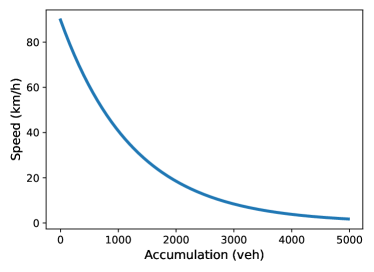
In this section, a case study on a small network is presented to evaluate the performance of the proposed control method. The structure of the small network is shown in Figure 6. There is one 3 km-long freeway with 4 on-ramps and 4 local urban areas in this network. We model the traffic dynamic of urban areas using the bathtub model, and the freeway and on-ramps are modeled using the ACTM. In bathtub models, the space-mean accumulation-speed diagram is modeled with a macroscopic Underwood’s model with a free-flow speed of 90 km/h and a critical accumulation of 1,265 vehicles. The MFD with macroscopic Underwood’s model is shown in Figure 7(a).

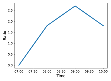
For the travel demand, we aim to simulate a 3-hour morning peak from 7:00 AM to 10:00 AM. The ratio of the demand pattern is shown in Figure 7(b), which means that the travel demand rises from 7:00 AM and reaches the peak at about 9:00 AM, then it falls to the normal demand level when the morning peak ends. The total generated travel demand in the morning peak is 47,271 vehicles.

Figure 6: The topology sketch of the small network in case study #1 (4 on-ramps and 4 perimeters).

(a) The sketch of the MFD for all bathtub models.

(b) The ratio of travel demand for each OD pair.

Figure 7: The road and demand information in the case study #1.

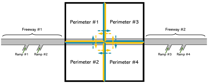
There are 8 agents in this small network for the 4 on-ramps and 4 perimeters. Due to the high dimension of the joint parameter space of the coordinated ALINEA and Gating, it is unrealistic to simultaneously search the best parameters for each ALINEA and Gating to achieve a global minimal TTT. Hence, the optimal demonstrators’ parameters of ALINEA and Gating for 4 on-ramps and 4 perimeters are finetuned using the grid search method respectively. However, in the proposed DRL method, all agents are simultaneously trained to ensure collaborations among agents to achieve a smaller TTT.

In this study, the TTT is used as the objective of the DRL. Other quantities, including average trip speed and delay, are also important to measure the control effects of the control method. The average trip speed is computed as the mean of average speeds for all trips, and the delay is calculated as the ratio of the gaps between free-flow TTT and current TTT over the free-flow TTT. Furthermore, we compared the proposed model with the no control, demonstrators (ALINEA or Gating), and other baseline methods, such as DAgger, DQN and DRQN. DAgger (Ross et al. 2011) is an imitation learning algorithm that iteratively learns deterministic policies from a prepared generated dataset. DQN (Mnih et al. 2015) is a classic DRL method for discrete control and fully observable problem. DRQN (Hausknecht and Stone 2015) is a DRL method focusing on solving discrete control and POMDPs using historical information.

4.2.1 Experimental results and comparisons

In addition to the coordinated ramp metering and perimeter control, we also set 2 other control scenarios, ramp-only and perimeter-only. In each control scenario, we trained each model 5 times with different random seeds individually to examine the robustness of the proposed model. The performance of the proposed methods and other baseline methods are shown in Table 2. If ramps and perimeters are not controlled, the normal average travel time for each traveler is 3,783.93 seconds, and the average delay is 6.69, meaning that the actual travel time is 6.69 times the TTT in free-flow conditions. The average speed for each trip is 30.52 km/h. Typically, in the coordinated ramp metering and perimeter control, if they are controlled by the proposed method, the TTT can be decreased by 31.3%, the delay can be reduced to 4.28, and the average trip speed can increase by 6.7%. The proposed method reaches the minimal TTT and delay in each control scenario, and achieves the highest average speed except in the perimeter-only scenario. One can see the proposed DRL can outperform the teachers (i.e., demonstrators) by 46.1% in TTT. Compared to DAgger, DQN, and DRQN, the proposed method can not only learn the pre-determined control strategy, but also explore a better policy based on the knowledge it has learned. This demonstrates the necessity of both demonstration and exploration. Importantly, the result in coordinated ramp metering and perimeter control is better than the results in the ramp-only and perimeter-only with respect to the TTT and delay. It indicates that the simultaneous control of freeways and urban areas can indeed enhance traffic efficiency for the entire network.

Control	Model	Reward	TTT (s)	Delay	Speed (km/h)
No Control		3783.93	6.69	30.52
Ramp	Demonstrator	824.61	2959.31	5.02	33.55
	DAgger	925.27 $\pm$ 164.11	2858.65 $\pm$ 164.11	4.81 $\pm$ 0.33	33.81 $\pm$ 0.28
	DQN	848.20 $\pm$ 88.97	2935.71 $\pm$ 88.97	4.97 $\pm$ 0.18	31.96 $\pm$ 1.34
	DRQN	895.30 $\pm$ 54.45	2888.61 $\pm$ 54.45	4.87 $\pm$ 0.11	31.93 $\pm$ 0.23
	Proposed	959.94 $\pm$ 30.07	2823.97 $\pm$ 30.07	4.74 $\pm$ 0.06	33.99 $\pm$ 0.14
Perimeter	Demonstrator	566.27	3217.64	5.54	31.66
	DAgger	132.35 $\pm$ 156.25	2651.57 $\pm$ 156.25	6.43 $\pm$ 0.31	31.01 $\pm$ 0.40
	DQN	89.78 $\pm$ 330.28	3694.13 $\pm$ 330.28	6.51 $\pm$ 0.67	30.39 $\pm$ 0.24
	DRQN	311.87 $\pm$ 66.86	3472.05 $\pm$ 66.86	6.06 $\pm$ 0.13	30.20 $\pm$ 0.92
	Proposed	597.48 $\pm$ 13.74	3186.44 $\pm$ 13.74	5.48 $\pm$ 0.01	31.48 $\pm$ 0.28
Ramp & Perimeter	Demonstrator	811.28	2972.64	5.04	31.06
	DAgger	805.93 $\pm$ 134.80	2977.98 $\pm$ 134.80	5.05 $\pm$ 0.27	31.86 $\pm$ 1.40
	DQN	424.36 $\pm$ 596.62	3359.56 $\pm$ 596.62	5.83 $\pm$ 1.21	29.65 $\pm$ 2.06
	DRQN	848.12 $\pm$ 247.15	2935.80 $\pm$ 247.15	4.97 $\pm$ 0.50	31.29 $\pm$ 2.90
	Proposed	1185.08 $\pm$ 98.74	2598.83 $\pm$ 98.74	4.28 $\pm$ 0.20	32.58 $\pm$ 0.96

Table 2: The comparison of the control performance with different methods under different scenarios (mean $\pm$ std for 5 random runs).

The reward curves of the DQN, DRQN, and the proposed DRL method in the training stage are shown in Figure 8. It can be seen that the reward of the proposed model is higher than that of DQN and DRQN most time in the training stage. The cumulative reward gradually increased and reached a peak of 1200 at about Epoch # 80, while the cumulative reward of DQN and DRQN may reach a maximum of 500.

Figure 8: The reward curves of the DQN, DRQN and the proposed method in the training stage.

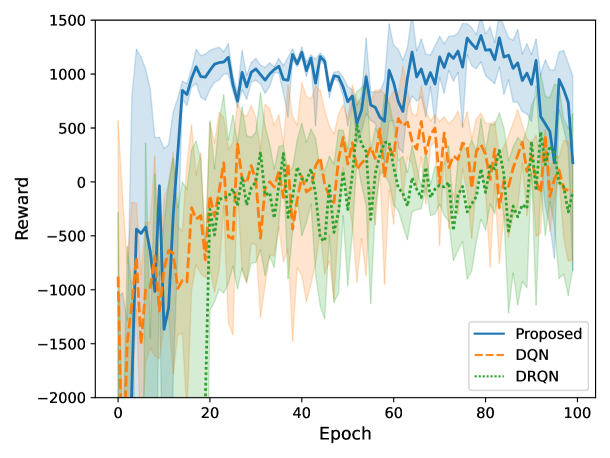
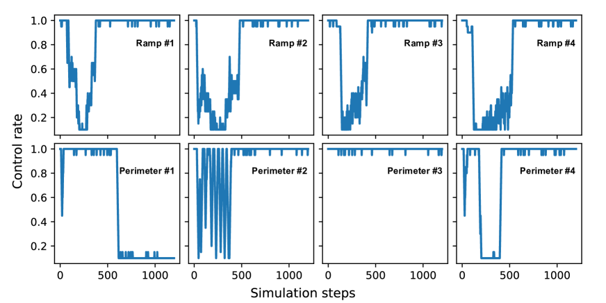
Figure 9 shows the control rate variation of ramps and perimeters with the proposed method. Here we set $\mathbf{u}_{min}$, $\mathbf{U}_{min}$ and $\mathbf{u}_{max}$, $\mathbf{U}_{max}$ as $0.1$ and $1$. It can be seen that all ramps share a similar control pattern where ramps keep open when the freeways are not in congestion, and the metering rate drops drastically to the minimal capacity when ramps are queued to maintain the throughput of freeways. Once the peak hours end, ramps restore to be fully open. The control strategies are different for perimeters. Perimeter #1 and #3 remain open, and the control rate of Perimeter #2 fluctuates when the urban area is in congestion, which resembles the patterns of bang-bang control. It may be interpreted that this urban area is sensitive to accumulation variation. Excess vehicle accumulation may result in serious congestion in downstream freeways and urban areas.

Figure 9: The control rate variation for all controllable ramps and perimeters in case study #1.

The evolution of traffic densities on freeways and vehicle accumulation in urban areas are shown in Figures 10 and 11. In order to better visualize the result, we select 2 road segments on the freeway and named them as Freeway #1 and Freeway #2, respectively. Ramp #1 and #2 are located at the first 1km and 2km of the Freeway #1 while Ramp #3 and #4 are at the first 1km and 2km of the Freeway #2. Figure 10(a) shows the evolution of traffic density on Freeway #1 with no control regime, demonstrator (i.e., ALINEA) and the proposed method. It can be seen that if ramps are not controlled, initially, the congestion emerges at Ramp #2 from around 8:00 AM, then it spills back rapidly to Ramp #1. At around 8:20 AM, the congestion spreads to the origin of the freeway. This scenario is highly congested since the traffic density in peak hours surpasses 200 veh/km/lane from the origin of the freeway to Ramp #1, and surpasses 150 veh/km/lane from Ramp #1 to #2. The road segment from Ramp #2 to the destination of the freeway is not affected by the traffic congestion at ramps since vehicles are most blocked at Ramp #1 and Ramp #2, and no congestion spills back from the destination of the freeway. Hence vehicles run with the free-flow speed in this road segment. The congestion from Ramp #1 to Ramp #2 ends at around 10:00 AM, and the accumulated vehicles on mainlines begin to move. However, the congestion from the origin of the freeway to Ramp #2 extends for extra 40 minutes since the remaining queuing vehicles at Ramp #1 still affect the traffic throughput on the mainline. All vehicles on Freeway #1 have been moved out at about 11:40 AM, and the congestion time lasted for about 3 hours. If Ramp #1 and #2 are controlled by the demonstrator or the proposed method, it can be seen that congestion rarely exists on Freeway #1. Most time, the traffic density will not exceed 100 veh/km/lane everywhere on the freeway. It means that control methods can significantly ease traffic congestion and reduce the TTT for each traveler. If ramps are controlled with demonstrators, all vehicles on freeways are wiped out at about 11:40 AM, while all vehicles on freeways leave at about 11:30 AM. In contrast, if ramps are controlled with the proposed DRL method, the clearance time is 10 minutes ahead of the case with demonstrators. The evolution of traffic density on Freeway #2 shares a similar case with the one on Freeway #1, and detailed descriptions are omitted.

(a) Traffic density on Freeway #1 with different control methods. (unit: veh/km/lane)

(b) Traffic density on Freeway #2 with different control methods. (unit: veh/km/lane)

Figure 10: Traffic density on freeways with different control methods. For Freeway #1 and #2, there are two ramps located at the 1km and 2km of freeways.

(a) Vehicle accumulation in Region #1

(b) Vehicle accumulation in Region #3

(c) Vehicle accumulation in Region #2

(d) Vehicle accumulation in Region #4

Figure 11: Vehicle accumulation in different regions.

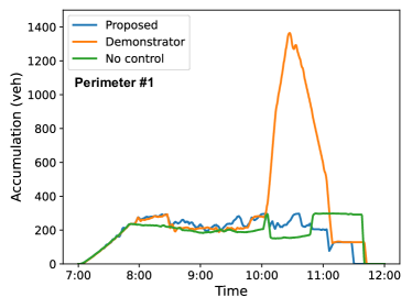
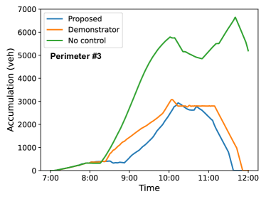
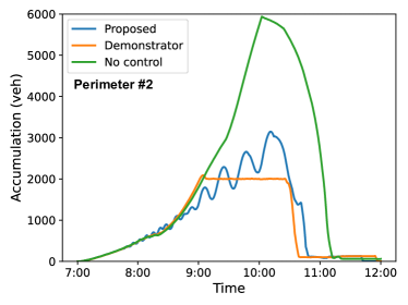
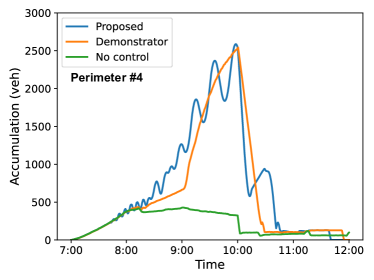
The vehicle accumulation in all regions is shown in Figure 11. If perimeters are not controlled, vehicles are prone to retain in Region #2 and Region #3. In Region #2, the level of congestion reaches a peak at around 10:00 AM and 6,000 vehicles are trapped in the region. Note that the vehicle accumulation in Region #2 and Region #3 is far beyond the total road capacity in a region (3,200 - 4,000 per region), causing a vicious circle of traffic congestion. Based on the MFD, if the current vehicle accumulation exceeds the critical vehicle accumulation, the average speed for all vehicles in the region decreases, and the outflow from the current region reduces consequently. However, the inflow vehicles are not limited unless the vehicle accumulation reaches the boundary capacity. The newborn trips will enlarge the vehicle accumulation and deteriorate the average speed again, which forms a circle. Moreover, the inconsistent uniform distribution of vehicle accumulation among all regions restricts the efficiency of the whole network. While Region #2 and Region #3 are in over-saturation, a few vehicles run in Region #1 and Region #4. If parts of vehicles in Region #2 and #3 can be balanced in Region #1 and Region #4 temporally, the traffic efficiency in the whole network may be enhanced. If perimeters are controlled by the demonstrator or the proposed method, Region #4 helps to withhold parts of vehicles so that Region #2 and #3 can achieve a higher traffic throughput. Controlled by the demonstrator, Region #1 even helps to retain parts of vehicles. However, the demonstrators did not fulfill a better control performance which may be due to the impact of Freeway #1 and #2. The proposed DRL method learns an implicit collaboration between ramps and perimeters which makes the traffic more efficient.

An interesting observation is that the variation of vehicle accumulation in Region #2 and Region #4 under the control of the proposed method forms the shape of waves, which is caused by the variation of control rate in Region #2. In Figure 9, the proposed method outputs a control strategy that resembles bang-bang control in Region #2. If Region #2 only allows the minimal traffic flow, Region #4, as an upstream region, will accumulate vehicles, and Region #2 will eject vehicles in the opposite manner. The variation of vehicle accumulation forms an ascending wave from 8:00 AM to 10:00 AM due to the newborn trips, and the follow-up phases form the opposite wave. The vehicle accumulation in Region #1 and Region #3 is not affected by Region #2 since Region #2 works like a buffer that flattens the traffic outflow into Region #1.

4.2.2 Ablation study

To validate the function of each component in the proposed DRL method, we present three groups of ablated models: no multi-step returns, no demonstrators, and no multi-step returns with demonstrators. The results for each group are shown in Table 3. Both the demonstrator and multi-step returns are essential to the proposed model. However, the utilization of demonstrators is more important than that of multi-step returns, which further verifies the necessity of demonstrators. The control performance is further deteriorated if neither demonstrator nor multi-step returns are used, which is equal to the DRQN model.

Model	Reward	TTT	Delay	Speed
Proposed	1185.08 $\pm$ 98.74	2598.83 $\pm$ 98.74	4.28 $\pm$ 0.20	32.58 $\pm$ 0.96
No nsteps	1125.91 $\pm$ 105.36	2658.00 $\pm$ 105.36	4.40 $\pm$ 0.21	31.97 $\pm$ 0.49
No demonstrator	892.21 $\pm$ 171.41	2891.70 $\pm$ 171.41	4.88 $\pm$ 0.34	30.01 $\pm$ 1.86
No demonstrator & nsteps	848.12 $\pm$ 247.15	2935.80 $\pm$ 247.15	4.97 $\pm$ 0.50	31.29 $\pm$ 2.90

Table 3: The ablation study for the coordinated control in the small network (mean $\pm$ std for 5 random runs).

4.2.3 Sensitivity analysis

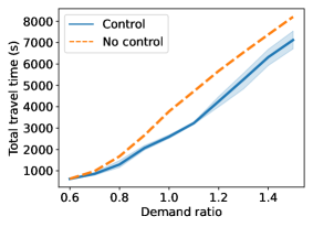
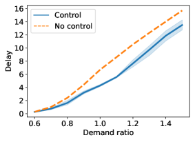
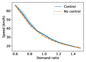
When we enact a control strategy in an urban network, the robustness of the control method is one of the most important issues to consider since the daily travel demand may vary randomly and the proposed method should be suitable for various traffic scenes. Hence we test the proposed model trained with the normal demand profile directly in different demand profiles without extra training 5 times. In different demand profiles, the OD pairs keep unchanged, while the volume in each demand record ranges from 60% to 150% of the normal demand. The comparison of performances between the control and no control methods are shown in Figure 12. When the travel demand reduces to 60% of the normal demand in the morning peak, it can be seen that there is nearly no difference in TTT, delay and speed between the control and no control methods. However, when the travel demand increases, the gaps in TTT and delay between the no control and the proposed method enlarges gradually and reaches the maximum when the demand ratio is 1.1. Then two lines of TTT and delay remain parallel from 1.1 to 1.5 since the traffic is over-congested and the traffic control efficiency is stablized.

(a) Total Travel Time

(b) Delay

(c) Speed

Figure 12: Sensitivity analysis with different demand profiles.

4.3 Case study #2: A real-world large-scale network

To further evaluate the performance of the proposed DRL method on a large-scale network, we implement the coordinated ramp metering and perimeter control on a real-world road network in the Kowloon district, Hong Kong SAR, China. The non-stationary properties of the environment in large-scale networks may be more challenging for the DRL method than in small networks. Hence the training epoch is set to 200, and other hyperparameters are the same as those in case study #1. The preparation for different parameter settings for the real-world network model is introduced as follows.

(a) The Kowloon District in the OpenStreetMap.

(b) The controllable agent in Kowloon District. The blue polygons represent perimeter agents, while red dots mean ramp agents.

(c) The partitioned urban areas simulated with the bathtub model in Kowloon District.

(d) The freeways simulated with the ACTM in Kowloon.

Figure 13: Overview of the study area.

Network data

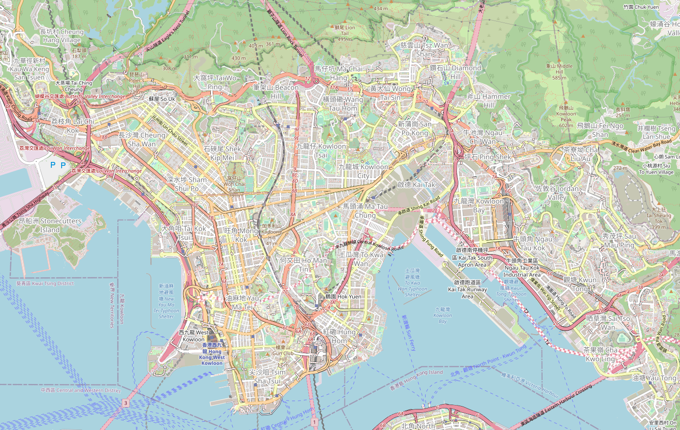
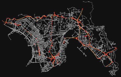
The road network is constructed from the OpenStreetMap (OSM, shown in Figure 13(a)) with OSMnx (Boeing 2017), which can convert the OSM into a directed graph. It can also correct broken links and delete non-junction nodes for network consolidation. The processed road network consists of 4,054 nodes and 7,385 edges. The speed limit and road capacity are acquired based on the road level, lane number, and jam density from the OSM attributes.

Network cluster profile

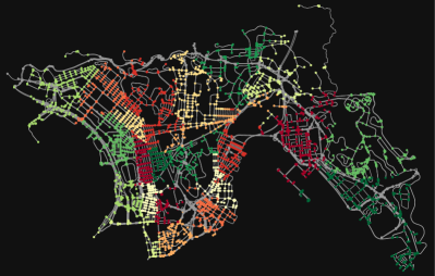
The network is partitioned into freeways (including ramps) and urban areas based on the road attributes in the OSM. For urban areas, we further split into several homogeneous regions to ensure a uniform relationship of MFD. The Leiden algorithm (Traag et al. 2019), which is a community detection algorithm, is adopted for the split. A total of 29 regions are obtained, in which 28 regions are urban areas simulated with the generalized bathtub model (shown in Figure 13(c)), and one region contains freeways and ramps that are modeled by the ACTM (shown in Figure 13(d)).

MFD parameters

The MFD for each region is acquired through the regional network topology. Recent work (Wong et al. 2021) reveals a relationship between the topology of the network and the macroscopic Underwood’s model using the taxi data in the Kowloon district, which is formulated in Equation 25.

$$v=53.874\cdot\exp(-0.077\gamma_{d})\cdot\exp\left(\frac{-k}{3.161\times 10^{6}/Deg_{t}}\right),$$ (25)

where $v$ is the average density and $k$ is the vehicle density in this region, $\gamma_{d}$ represents the number of junctions per kilometer, and degree density $Deg_{t}$ represents the average node degree per square kilometer.

Time-of-day OD demand

The time-of-day OD demand data is requested from the TomTom Move. The study area contains 135 OD regions, and we use the average OD demand in the morning peak (7:00 AM to 10:00 AM) for 30 days as the demand. There are a total of 228,306 trips in the morning peaks, and the visualization of the spatial OD flow for each hour is shown in Figure 14.

Figure 14: The hourly OD demand profile from 7:00 AM to 10:00 AM. Darker color indicates more trips between the OD pair.

4.3.1 Experimental results

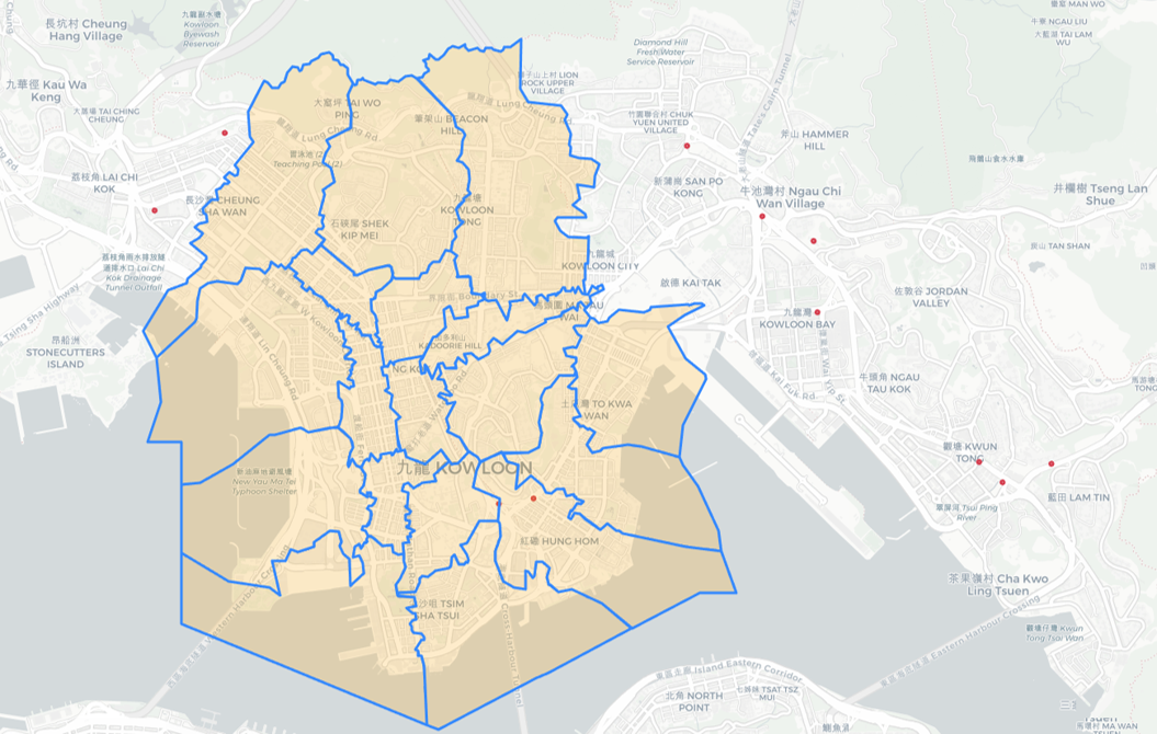
There are 29 agents in the study area: 11 of them are ramps and 18 of them are perimeters. The location of ramps and perimeters are shown in Figure 13(b). The blue borough represents the perimeter and the red dot denotes the ramp. The comparison of the control performance with different methods is shown in Table 4. The average travel time is around 33 minutes without any control method. If ramps and perimeters are controlled with the proposed method, each traveler can save extra 3 minutes on roads, accounting for a 7.8% reduction in TTT and a 6.1% increase in average trip speed. Compared to demonstrators (ALINEA and Gating), the proposed DRL method can reduce the TTT further by 12.9%. On the scope of the real-world and large-scale network, the proposed control method significantly improves the network efficiency.

Control	Model	Reward	TTT	Delay	Speed
No Control	None	2059.38	10.15	23.10
Ramp & Perimeter	Demonstrator	142.40	1896.21	9.27	24.50
	DAgger	135.75 $\pm$7.70	1903.79 $\pm$ 8.78	1.21 $\pm$ 0.01	24.13 $\pm$ 0.35
	DQN	132.46 $\pm$9.82	1907.54 $\pm$ 11.19	1.22 $\pm$ 0.01	23.21 $\pm$ 0.32
	DRQN	140.53 $\pm$ 8.29	1898.48 $\pm$ 9.32	1.20 $\pm$ 0.01	23.54 $\pm$ 0.47
	Proposed	160.84 $\pm$ 4.00	1875.48 $\pm$ 4.61	1.18 $\pm$ 0.00	24.53 $\pm$ 0.10

Table 4: The comparison of the control performance with different methods under different scenarios (mean $\pm$ std for 5 random runs).

5 Conclusion

In this paper, we propose a meso-macro dynamic traffic network model and a demonstrated-guided DRL method for coordinated ramp metering and perimeter control in large-scale networks. For the meso-macro traffic modeling, we integrate the ACTM and the generalized bathtub model to achieve multi-resolution and high efficiency in modeling large-scale networks. For the coordinated control, when we aim to control multiple agents in a complex environment simultaneously, the non-stationary environment makes it difficult for the DRL method to learn an effective policy. Hence we leverage demonstrators, (e.g., concise traditional controllers) to guide the DRL methods to stabilize the training of multiple agents.

The proposed DRL-based control framework has been evaluated in two case studies, a small network and a real-world and large-scale network in the Kowloon district, Hong Kong. For both case studies, the proposed method is compared with existing baselines, and it outperforms the demonstrators and existing DRL methods. In case study #1, the result shows that it can save 31.3% TTT for each traveler. We further conduct an ablation study and a sensitivity analysis to validate the function of each component and the robustness of the proposed DRL method. In case study #2, we apply the proposed method in a real-world large-scale network. The results show that it can save 7.8% TTT for each traveler, and compared to the demonstrator, the control performance can be further enhanced by 12.9% based on the TTT. Both case studies demonstrate the great potential of using demonstrators’ guidance in DRL training.

In future research, more extensions regarding the DRL method can be made based on the current study. For example, we can consider the explicit communication between ramps and perimeters in a large-scale control, which is important in Multi-agent Reinforcement Learning (MARL), and each agent may further explore a better control strategy by receiving messages from other agents. A simple DRL method can be the demonstrator of complex DRL methods, so we can adopt the concept of knowledge distillation to design a self-evolving DRL-based controller. Moreover, it would be practical to study whether the developed DRL can be generalizable for different network topologies and traffic scenarios in the real world.

Appendix A Notations

Meso-macro traffic modeling
$\mathbf{G}$	The traffic network.
$\mathbf{G}_{i}$	The network of region $i$.
$\mathbf{V}$	The node set of the traffic network.
$\mathbf{V}_{i}$	The node set of region $i$ in the traffic network.
$\mathbf{E}$	The link set (road set) of the traffic network.
$\mathcal{N}_{d}$	The number of regions in the traffic network.
$e_{r,s}$	The road from node $r$ to node $s$.
$l_{r,s}$	The length of road $l_{r,s}$.
$\mathcal{D}_{r,s}(t)$	The demand of road $e_{r,s}$.
$\mathcal{S}_{r,s}(t)$	The supply of road $e_{r,s}$.
$\delta_{r,s}$	The length of cell on road $e_{r,s}$.
$v_{r,s}^{max}$	The free-flow speed of road $e_{r,s}$.
$n_{r,s}^{k}(t)$	The vehicle number in the $k$th cell of road $e_{r,s}$.
$\hat{n}_{r,s}(t)$	The jam density of road $e_{r,s}$.
$f_{r,s}^{k,k+1}(t)$	The internal flow from cell $k$ to cell $k+1$ on road $e_{r,s}$.
$R_{r,s}^{k}(t)$	The on-ramp flow on the $k$th cell of road $e_{r,s}$.
$S_{r,s}^{k}(t)$	The off-ramp flow on the $k$th cell of road $e_{r,s}$.
$\mu_{r,s}(t)$	The number of trip begun on road $e_{r,s}$.
$\nu_{r,s}(t)$	The number of trip ended on road $e_{r,s}$.
$\phi_{*,r,s}(t)$	The external traffic flow into road $e_{r,s}$.
$\phi_{r,s,*}(t)$	The exteral traffic flow from road $e_{r,s}$.
$\phi(\cdots)$	The external flow allocation that regulates traffic flow between different roads.
$\psi_{+}(r)$	The downstream nodes of node $r$.
$\psi_{-}(r)$	The upstream nodes of node $r$.
$w_{r,s}$	The spillback speed on road $e_{r,s}$.
$q_{r,s}^{max}$	The capacity of road $e_{r,s}$.
$\gamma$	The on-ramp flow blending parameter.
$\zeta$	The on-ramp flow allocation coefficient.
$c_{r^{\prime},s^{\prime}}(t)$	The capacity for on-ramp flow.
$\rho_{r,s}^{k}$	The ramp rate of the $k$th cell on road $e_{r,s}$.
$\beta_{r,s}^{k}(t)$	The off-ramp split factor of the $k$ cell on road $e_{r,s}$.
$\overline{N}_{d}(t)$	The vehicle accumulation in region $d$.
$\overline{\mathcal{U}}_{d}(t)$	The trip begun in region $d$.
$\overline{\mathcal{V}}_{d}(t)$	The trip finished in region $d$.
$\overline{\Phi}_{d,*}(t)$	The external traffic flow from region $d$.
$\overline{\Phi}_{*,d}(t)$	The external traffic flow to region $d$.
$\mathcal{U}_{d}(t,\xi)$	The trip begun in region $d$ with remaining distance of $\xi$.
$\Phi_{*,d}(t,\xi)$	The external traffic flow from region $d$ with remaining distance of $\xi$.
$V_{d}(t)$	The average speed in region $d$.
$\hat{V}_{d}(\cdot)$	The MFD of region $d$.
$L_{d}^{sum}$	The total road length in region $d$.
$L_{d}^{max}$	The length of the longest trajectory in region $d$.
$\hat{\Phi}(\cdots)$	The external traffic allocator that regulates the traffic flow between different regions.
$\mathfrak{D}_{d}(t)$	The demand of region $d$.
$\mathfrak{S}_{d}(t)$	The supply of region $d$.
$\Psi_{+}(d)$	The downstream regions of region $d$.
$\Psi_{-}(d)$	The upstream regions of region $d$.
$\hat{N}_{d}$	The jam vehicle accumulation in region $d$.
$C_{d,+}^{margin}$	The outflow capacity at the boundary of region $d$.
$C_{d,-}^{margin}$	The inflow capacity at the boudnary of region $d$.
$\mathcal{P}_{d}(t)$	The control rate of the perimeter of region $d$.
DRL method
$\mathcal{X}$	The state set.
$\mathcal{U}$	The action set.
$\mathcal{P}$	The state transition probability.
$\mathcal{R}$	The reward set.
$\Omega$	The observation set for an agent.
$\mathcal{O}$	The observation probability in the environment.
$\mathbf{x}_{t}$	The state.
$\mathbf{o}_{t}$	The observation.
$\mathbf{h}_{t}$	The historical information.
$\mathbf{u}_{t}$	The action.
$\mathbf{r}_{t}$	The reward.
$\hat{\mathbf{r}}_{t}^{i}(\eta)$	The multi-steps reward with a step size of $\eta$.
$G_{t}$	The discounted cumulative reward from time $t$.
$\lambda$	The discount factor.
$\mathcal{N}_{p}$	The number of total trips.
$T_{i}^{end}$	The end time for trip $i$.
$T_{i}^{start}$	The start time for trip $i$.
$T^{term}$	The termination time for the simulation.
$\mathcal{N}^{inj}(t)$	The number of injected vehicle.
$\mathcal{N}^{run}(t)$	The number of running vehicle.
$\mathcal{N}^{com}(t,t^{\prime})$	The number of completed vehicle from time $t$ to time $t^{\prime}$.
$C_{r}$	A normalization term for reward.
$KI_{r,s}^{k}$	The integral parameter in ALINEA.
$\dot{n}_{r,s}^{k}$	The threshold for the $k$th cell on road $e_{r,s}$ in ALINEA.
$KP_{d}$	The proportional parameter in Gating.
$KI_{d}$	The integral parameter in Gating.
$\dot{N}_{d}$	The threshold for the region $d$ in Gating.
$\eta$	The steps of rewards.
$Q(\cdots)$	The action value function.
$\pi(\cdots)$	The agent policy.
$\overline{\pi}(\cdots)$	The demonstrator policy.
$\pi(\cdots)$	The dummy policy.
$\mathcal{N}_{B}$	The replay buffer size.
$\mathcal{N}_{m}$	The epoch number.
$\mathcal{N}_{o}$	The period for training DRL methods.
$\mathcal{N}_{c}$	The period for cloning the source network.
$\epsilon_{start}$	The initial value of the $\epsilon$.
$\epsilon_{end}$	The final value of the $\epsilon$.
$\epsilon_{last}$	The duration of $\epsilon$ decayed in the training process.
$\alpha_{min}$	The minimal value that used to normalize the value of $\alpha_{t}$.
$\alpha_{step}$	The normalization term for the time $t$ in calculation of $\alpha_{t}$.
$\alpha_{term}$	The termination steps in calculation of $\alpha_{t}$.
$\alpha_{amp}$	The amplification of the KL divergence.

Appendix B Conservation law of different cells in ACTM

In this section, we present the conservation law of traffic dynamic in source cells, sink cells, general cells and off-ramp cells in the ACTM. To simplify the evolution of traffic flows, we made the following assumptions.

Assumption 1.

In the ACTM, a trip begins at the source cell and ends at the sink cell.

Assumption 2.

Any source cells and sink cells are not connected with on-ramp entrances or off-ramp exits.

Based on these assumptions, the conservation law of traffic flow in source cells, sink cells, general cells, and off-ramp cells can be discussed separately.

The conservation law of a source cell

In a source cell, there is no internal flow into the source cell since it is the first cell on the road. The conservation law of vehicles in the source cell is formulated in Equation 26,

$$n_{r,s}^{1}(t) =n_{r,s}^{1}(t-1)+\mu_{r,s}(t)+\phi_{*,r,s}(t)-f_{r,s}^{1,2}(t)$$ (26)

$$\phi_{*,r,s}(t) =\sum_{i\in\psi^{-}(r)}\phi_{i,r,s}(t)$$

$$\phi_{i,r,s}(t) =\hat{\phi}\left(\left\{\mathcal{D}_{j,r}(t)|\forall j\in\psi^{-}(r)\right\},\left\{\mathcal{S}_{r,k}(t)|\forall k\in\psi^{+}(r)\right\}\right),$$

$$\qquad\qquad\qquad\forall r,s\in\mathbf{V}$$

where $n_{r,s}^{1}(t)$ is the vehicle number in the source cell at time $t$, $f_{r,s}^{1,2}$ is the internal traffic flow from the first cell (source cell) to the second cell on road $e_{r,s}$ at time $t$. $\phi_{i,r,s}(t)$ denotes the external traffic flow from road $e_{i,r}$ into road $e_{r,s}$. $\psi_{r}^{-}$ and $\psi_{r}^{+}$ mean sets of upstream and downstream nodes that directly connects to node $r$ respectively. $\hat{\phi}(\cdots)$ represents a function that allocates the external flows between different roads by randomly transferring vehicles from the sink cell of the upstream road to the source cell of the downstream road. $\mathcal{D}_{j,r}$ is demand on road $e_{j,r}$ at time $t$, and $\mathcal{S}_{r,k}$ is the supply on road $e_{r,k}$ at time $t$. The demand and supply are calculated as

$$\mathcal{D}_{r,s}(t) =\min\left\{n_{r,s}^{-1}(t)-\nu_{r,s}(t),q_{r,s}^{max}\right\}$$ (27)

$$\mathcal{S}_{r,s}(t) =\min\left\{\frac{w_{r,s}}{v_{r,s}^{max}}\left(\hat{n}_{r,s}-n_{r,s}^{-1}(t)-\mu_{r,s}(t)\right),q_{r,s}^{max}\right\}$$

The conservation law of a sink cell

In a sink cell, there is no internal flow from the sink cell since it is the last cell on the road. The conservation law of vehicles in the sink cell is formulated in Equation 28,

$$n_{r,s}^{-1}(t) =n_{r,s}^{-1}(t-1)-\nu_{r,s}(t)-\phi_{r,s,*}(t)+f_{r,s}^{-2,-1}(t)$$ (28)

$$\phi_{r,s,*}(t) =\sum_{i\in\psi^{+}(s)}\phi_{r,s,i}(t)$$

$$\phi_{r,s,i}(t) =\hat{\phi}\left(\left\{\mathcal{D}_{j,s}(t)|\forall j\in\psi^{-}(s)\right\},\left\{\mathcal{S}_{s,k}(t)|\forall k\in\psi^{+}(s)\right\}\right),$$

$$\qquad\qquad\qquad\forall r,s\in\mathbf{V}$$

where $n_{r,s}^{-1}(t)$ is the vehicle number in the sink cell at time $t$, $f_{r,s}^{-2,-1}$ is the internal traffic flow from the second to last cell to the last cell (sink cell) on road $e_{r,s}$ at time $t$. The external flow of road $e_{r,s}$, $\phi_{r,s,*}$ will be distributed to downstream roads through the external flow regulator.

The conservation law of a general cell

In general cells, there is no external traffic flow, and trip source or sink. Hence we only consider the internal flows from on-ramps to mainlines, mainlines to mainlines and mainlines to off-ramps.

The conservation law of a general cell is modeled in Equation 29,

$$n_{r,s}^{k}(t) =n_{r,s}^{k}(t-1)+f_{r,s}^{k-1,k}(t)-f_{r,s}^{k,k+1}(t)+R_{r,s}^{k}(t)-S_{r,s}^{k}(t)$$ (29)

$$f_{r,s}^{k,k+1}(t) =\min\left\{v_{r,s}^{max}\left(1-\beta_{r,s}^{k}(t)\right)\left(n_{r,s}^{k}(t)+\gamma R_{r,s}^{k}(t)\right),w_{r,s}\left(\hat{n}_{r,s}-n_{r,s}^{k+1}(t)-\gamma R_{r,s}^{k+1}(t)\right),q_{r,s}^{max}\right\},$$

$$\qquad\qquad\qquad\qquad\forall r,s\in\mathbf{V},\ 2\leq k\leq\lceil l_{r,s}/\delta_{r,s}\rceil-1,$$

where $w_{r,s}$ is the spillback speed of congestion at road $e_{r,s}$, $\beta_{r,s}^{k}(t)$ is the split ratio for off-ramp in cell $k$ on road $e_{r,s}$. $\gamma$ is the on-ramp flow blending parameter determined how much of the on-ramp flow is added to the mainstream before the mainstream arrives, which indicates the impact of mainstream from on-ramp flows, $\hat{n}_{r,s}$ is the jam density on road $e_{r,s}$.

It can be seen that the mainstream $f_{r,s}^{k,k+1}(t)$ should fulfill the following conditions.

$$f_{r,s}^{k,k+1}(t)+S_{r,s}^{k}(t) \leq v_{r,s}^{max}\left(n_{r,s}^{k}(t)+\gamma R_{r,s}^{k}(t)\right)$$ (30)

$$f_{r,s}^{k,k+1}(t) \leq w_{r,s}\left(\hat{n}_{r,s}-n_{r,s}^{k+1}(t)-\gamma R_{r,s}^{k+1}(t)\right)$$ (31)

$$f_{r,s}^{k,k+1}(t) \leq q_{r,s}^{max}(t)$$ (32)

Equation 30 restricts that the average speed of total vehicles left cell $k$ should under the free-flow speed. Equation 31 limits that the mainstream to the next cell should not exceed the supply of the next cell. Equation 32 ensures that the mainstream should not surpass the road capacity.

The conservation law of an off-ramp cell

For an off-ramp cell, the conservation law is formulated in Equation 33,

$$n_{r^{\prime\prime},s^{\prime\prime}}^{1}(t) =n_{r^{\prime\prime},s^{\prime\prime}}^{1}(t-1)-f_{r^{\prime\prime},s^{\prime\prime}}^{1,2}(t)+S_{r,s}^{k}(t)$$ (33)

$$S_{r,s}^{k}(t) =\frac{\beta_{r,s}^{k}(t)}{1-\beta_{r,s}^{k}(t)}f_{r,s}^{k,k+1}(t),$$

$$\forall r,s\in\mathbf{V},\ k\leq\lceil l_{r,s}/\delta_{r,s}\rceil,$$

where $n_{r^{\prime\prime},s^{\prime\prime}}^{1}(t)$ is the vehicle number in the first cell of road $e_{r^{\prime\prime},s^{\prime\prime}}$, the off-ramp of road $e_{r,s}$. $S_{r,s}^{k}(t)$ is determined by the mainstream $f_{r,s}^{k,k+1}(t)$ and the split ratio of mainstream $\beta_{r,s}^{k}(t)$. In the meso-marco traffic modeling, the split ratio $\beta_{r,s}^{k}(t)$ varies according to the destination of vehicles in the cell.

Appendix C Demonstrators of agents

This section presents the detailed formulation for demonstrators on both freeways and local roads.

The demonstrator of a ramp

ALINEA is a local ramp metering algorithm that aims to regulate the ramp flow on a local bottleneck. For an on-ramp, ALINEA takes the traffic occupancy as the input, and outputs the metered flow, which can be fulfilled by changing the green and red time of the signal light at a ramp. To better combine the ALINEA with the proposed simulator, we change the unit of decision variables and parameters in the original ALINEA method. The modified ALINEA controller is shown in Equation 34,

$$\rho_{r,s}^{k}(t+1)=\rho_{r,s}^{k}(t)+KI_{r,s}^{k}\left(\dot{n}_{r,s}^{k}-n_{r,s}^{k}(t)\right),$$ (34)

where $\rho_{r,s}^{k}(t)$ is the metered rate of the $k$th ramp on the road $e_{r,s}$ defined in Equation 1. $n_{r,s}^{k}(t)$ is the vehicle number in the $k$th ramp on the road $e_{r,s}$. $\dot{n}_{r,s}^{k}$ is a threshold for the controlled vehicle number, which is usually the value of the critical density in the cell. $KI_{r,s}^{k}$ is a step-size parameter defined that how sensitive it reacts to traffic congestion. The larger the number is, the faster it delays vehicles on the ramp when the mainstream is congested, and vice versa.

The ALINEA is an adaptive local control method that performs differently according to the level of congestion. This study quantizes the control rate of ALINEA using a step size of $\Delta u$. By comparing to values in the threshold $\dot{n}_{r,s}^{k}$ and the vehicle number $n_{r,s}^{k}(t)$, the control action is calculated as follows:

$$\mathbf{u}_{t}=\begin{cases}+\Delta\mathbf{u},&\dot{n}_{r,s}^{k}-n_{r,s}^{k}(t)>0\\ 0,&\dot{n}_{r,s}^{k}-n_{r,s}^{k}(t)=0\\ -\Delta\mathbf{u},&\dot{n}_{r,s}^{k}-n_{r,s}^{k}(t)<0\\ \end{cases}.$$

The demonstrator of a perimeter

Gating is a local perimeter control method aiming to limit the traffic inflow into a congested urban area. For a perimeter, Gating takes the Total Time Spent (TTS) as the input, and outputs the inflow capacity at boundaries. Here the TTS refers to the number of vehicles in a region. The unit of decision variables and parameters in the original Gating method is also replaced to better fit this study. The modified Gating controller is shown in Equation 35:

$$\mathcal{P}_{d}(t+1)=\mathcal{P}_{d}(t)-KP_{d}\left(N_{d}(t+1)-N_{d}(t)\right)+KI_{d}\left(\dot{N}_{d}-N_{d}(t)\right),$$ (35)

where $\mathcal{P}_{d}(t)$ is the inflow rate of region $d$ in Equation 10, $N_{d}(t)$ is the vehicle accumulation in region $d$, $\dot{N}_{d}(t)$ is a threshold for the controlled vehicle accumulation. Typically, the threshold is set as the critical vehicle accumulation of the MFD in the region. $KP_{d}$ and $KI_{d}$ are regulator parameters that weigh the impact on the inflow rate from the historical and critical vehicle accumulation.

Gating is also an adaptive local control method that responds differently according to the congestion level, and its control rate is a continuous variable in the system. To discretize the Gating method, the control action is defined as follows:

$$\mathbf{u}_{t}=\begin{cases}+\Delta\mathbf{u},&KI_{d}\left(\dot{N}_{d}-N_{d}(t)\right)-KP_{d}\left(N_{d}(t+1)-N_{d}(t)\right)>0\\ 0,&KI_{d}\left(\dot{N}_{d}-N_{d}(t)\right)-KP_{d}\left(N_{d}(t+1)-N_{d}(t)\right)=0\\ -\Delta\mathbf{u},&KI_{d}\left(\dot{N}_{d}-N_{d}(t)\right)-KP_{d}\left(N_{d}(t+1)-N_{d}(t)\right)<0\\ \end{cases}.$$

References

- (1)
- Aboudolas and Geroliminis (2013) Aboudolas, K. and Geroliminis, N. (2013), ‘Perimeter and boundary flow control in multi-reservoir heterogeneous networks’, Transportation Research Part B: Methodological 55, 265–281.
-
Aimsun (2022)
Aimsun (2022), ‘Aimsun next’.
https://www.aimsun.com/ - Auld et al. (2016) Auld, J., Hope, M., Ley, H., Sokolov, V., Xu, B. and Zhang, K. (2016), ‘Polaris: Agent-based modeling framework development and implementation for integrated travel demand and network and operations simulations’, Transportation Research Part C: Emerging Technologies 64, 101–116.
- Bellemare et al. (2017) Bellemare, M. G., Dabney, W. and Munos, R. (2017), A distributional perspective on reinforcement learning, in D. Precup and Y. W. Teh, eds, ‘Proceedings of the 34th International Conference on Machine Learning’, Vol. 70 of Proceedings of Machine Learning Research, PMLR, pp. 449–458.
- Belletti et al. (2018) Belletti, F., Haziza, D., Gomes, G. and Bayen, A. M. (2018), ‘Expert level control of ramp metering based on multi-task deep reinforcement learning’, IEEE Transactions on Intelligent Transportation Systems 19(4), 1198–1207.
- Bernhard et al. (2020) Bernhard, J., Esterle, K., Hart, P. and Kessler, T. (2020), BARK: Open behavior benchmarking in multi-agent environments, in ‘2020 IEEE/RSJ International Conference on Intelligent Robots and Systems (IROS)’.
- Boeing (2017) Boeing, G. (2017), ‘OSMnx: New methods for acquiring, constructing, analyzing, and visualizing complex street networks’, Computers, Environment and Urban Systems 65, 126–139.
- Brockman et al. (2016) Brockman, G., Cheung, V., Pettersson, L., Schneider, J., Schulman, J., Tang, J. and Zaremba, W. (2016), ‘Openai gym’, arXiv preprint arXiv:1606.01540 .
- Cassidy and Bertini (1999) Cassidy, M. J. and Bertini, R. L. (1999), ‘Some traffic features at freeway bottlenecks’, Transportation Research Part B: Methodological 33(1), 25–42.
- Cassidy and Rudjanakanoknad (2005) Cassidy, M. J. and Rudjanakanoknad, J. (2005), ‘Increasing the capacity of an isolated merge by metering its on-ramp’, Transportation Research Part B: Methodological 39(10), 896–913.
- Chen et al. (2022) Chen, C., Huang, Y., Lam, W., Pan, T., Hsu, S., Sumalee, A. and Zhong, R. (2022), ‘Data efficient reinforcement learning and adaptive optimal perimeter control of network traffic dynamics’, Transportation Research Part C: Emerging Technologies 142, 103759.
- Daganzo (1994) Daganzo, C. F. (1994), ‘The cell transmission model: A dynamic representation of highway traffic consistent with the hydrodynamic theory’, Transportation Research Part B: Methodological 28(4), 269–287.
- Daganzo (1995) Daganzo, C. F. (1995), ‘The cell transmission model, part ii: Network traffic’, Transportation Research Part B: Methodological 29(2), 79–93.
- Daganzo (2007) Daganzo, C. F. (2007), ‘Urban gridlock: Macroscopic modeling and mitigation approaches’, Transportation Research Part B: Methodological 41(1), 49–62.
- Daganzo and Geroliminis (2008) Daganzo, C. F. and Geroliminis, N. (2008), ‘An analytical approximation for the macroscopic fundamental diagram of urban traffic’, Transportation Research Part B: Methodological 42(9), 771–781.
- Deng et al. (2019) Deng, F., Jin, J., Shen, Y. and Du, Y. (2019), Advanced self-improving ramp metering algorithm based on multi-agent deep reinforcement learning, in ‘2019 IEEE Intelligent Transportation Systems Conference (ITSC)’, pp. 3804–3809.
- Ding et al. (2021) Ding, H., Yuan, H., Zheng, X., Bai, H., Huang, W. and Jiang, C. (2021), ‘Integrated control for a large-scale mixed network of arterials and freeways’, IEEE Intelligent Transportation Systems Magazine 13(3), 131–145.
- Fares and Gomaa (2014) Fares, A. and Gomaa, W. (2014), Freeway ramp-metering control based on reinforcement learning, in ‘11th IEEE International Conference on Control & Automation (ICCA)’, pp. 1226–1231.
- Fares and Gomaa (2015) Fares, A. and Gomaa, W. (2015), Multi-agent reinforcement learning control for ramp metering, in H. Selvaraj, D. Zydek and G. Chmaj, eds, ‘Progress in Systems Engineering’, Springer International Publishing, Cham, pp. 167–173.
- Fortunato et al. (2017) Fortunato, M., Azar, M. G., Piot, B., Menick, J., Osband, I., Graves, A., Mnih, V., Munos, R., Hassabis, D., Pietquin, O. et al. (2017), ‘Noisy networks for exploration’, arXiv preprint arXiv:1706.10295 .
- Fu et al. (2017) Fu, H., Liu, N. and Hu, G. (2017), ‘Hierarchical perimeter control with guaranteed stability for dynamically coupled heterogeneous urban traffic’, Transportation Research Part C: Emerging Technologies 83, 18–38.
- Geroliminis and Daganzo (2008) Geroliminis, N. and Daganzo, C. F. (2008), ‘Existence of urban-scale macroscopic fundamental diagrams: Some experimental findings’, Transportation Research Part B: Methodological 42(9), 759–770.
- Gomes and Horowitz (2006) Gomes, G. and Horowitz, R. (2006), ‘Optimal freeway ramp metering using the asymmetric cell transmission model’, Transportation Research Part C: Emerging Technologies 14(4), 244–262.
- Haarnoja et al. (2018) Haarnoja, T., Zhou, A., Abbeel, P. and Levine, S. (2018), Soft actor-critic: Off-policy maximum entropy deep reinforcement learning with a stochastic actor, in ‘International conference on machine learning’, PMLR, pp. 1861–1870.
- Haddad et al. (2013) Haddad, J., Ramezani, M. and Geroliminis, N. (2013), ‘Cooperative traffic control of a mixed network with two urban regions and a freeway’, Transportation Research Part B: Methodological 54, 17–36.
- Han et al. (2022) Han, Y., Wang, M., Li, L., Roncoli, C., Gao, J. and Liu, P. (2022), ‘A physics-informed reinforcement learning-based strategy for local and coordinated ramp metering’, Transportation Research Part C: Emerging Technologies 137, 103584.
- Hausknecht and Stone (2015) Hausknecht, M. and Stone, P. (2015), ‘Deep recurrent q-learning for partially observable mdps’, arXiv preprint arXiv:1507.06527 .
- Hegyi et al. (2005) Hegyi, A., De Schutter, B. and Hellendoorn, H. (2005), ‘Model predictive control for optimal coordination of ramp metering and variable speed limits’, Transportation Research Part C: Emerging Technologies 13(3), 185–209.
- Hessel et al. (2018) Hessel, M., Modayil, J., Van Hasselt, H., Schaul, T., Ostrovski, G., Dabney, W., Horgan, D., Piot, B., Azar, M. and Silver, D. (2018), Rainbow: Combining improvements in deep reinforcement learning.
- Hester et al. (2017) Hester, T., Vecerik, M., Pietquin, O., Lanctot, M., Schaul, T., Piot, B., Horgan, D., Quan, J., Sendonaris, A., Dulac-Arnold, G., Osband, I., Agapiou, J., Leibo, J. Z. and Gruslys, A. (2017), ‘Deep q-learning from demonstrations’.
- Horni et al. (2016) Horni, A., Nagel, K. and Axhausen, K. W. (2016), The Multi-Agent Transport Simulation MATSim, Ubiquity Press, London, GBR.
- Hu et al. (2022) Hu, Z., Zhuge, C. and Ma, W. (2022), Towards a very large scale traffic simulator for multi-agent reinforcement learning testbeds, in ‘2022 IEEE 25th International Conference on Intelligent Transportation Systems (ITSC)’, IEEE, pp. 363–368.
- Huang et al. (2022) Huang, Z., Wu, J. and Lv, C. (2022), ‘Efficient deep reinforcement learning with imitative expert priors for autonomous driving’, IEEE Transactions on Neural Networks and Learning Systems pp. 1–13.
- Jin (2020) Jin, W.-L. (2020), ‘Generalized bathtub model of network trip flows’, Transportation Research Part B: Methodological 136, 138–157.
- Keyvan-Ekbatani et al. (2012) Keyvan-Ekbatani, M., Kouvelas, A., Papamichail, I. and Papageorgiou, M. (2012), ‘Exploiting the fundamental diagram of urban networks for feedback-based gating’, Transportation Research Part B: Methodological 46(10), 1393–1403.
- Keyvan-Ekbatani, Papageorgiou and Knoop (2015) Keyvan-Ekbatani, M., Papageorgiou, M. and Knoop, V. L. (2015), ‘Controller design for gating traffic control in presence of time-delay in urban road networks’, Transportation Research Part C: Emerging Technologies 59, 308–322. Special Issue on International Symposium on Transportation and Traffic Theory.
- Keyvan-Ekbatani et al. (2013) Keyvan-Ekbatani, M., Papageorgiou, M. and Papamichail, I. (2013), ‘Urban congestion gating control based on reduced operational network fundamental diagrams’, Transportation Research Part C: Emerging Technologies 33, 74–87.
- Keyvan-Ekbatani, Yildirimoglu, Geroliminis and Papageorgiou (2015) Keyvan-Ekbatani, M., Yildirimoglu, M., Geroliminis, N. and Papageorgiou, M. (2015), ‘Multiple concentric gating traffic control in large-scale urban networks’, IEEE Transactions on Intelligent Transportation Systems 16(4), 2141–2154.
- Lei et al. (2020) Lei, T., Hou, Z. and Ren, Y. (2020), ‘Data-driven model free adaptive perimeter control for multi-region urban traffic networks with route choice’, IEEE Transactions on Intelligent Transportation Systems 21(7), 2894–2905.
- Li and Hou (2021) Li, D. and Hou, Z. (2021), ‘Perimeter control of urban traffic networks based on model-free adaptive control’, IEEE Transactions on Intelligent Transportation Systems 22(10), 6460–6472.
- Liang et al. (2022) Liang, C., Huang, Z., Liu, Y., Liu, Z., Zheng, G., Shi, H., Du, Y., Li, F. and Li, Z. (2022), ‘Cblab: Scalable traffic simulation with enriched data supporting’.
- Lillicrap et al. (2015) Lillicrap, T. P., Hunt, J. J., Pritzel, A., Heess, N., Erez, T., Tassa, Y., Silver, D. and Wierstra, D. (2015), ‘Continuous control with deep reinforcement learning’, arXiv preprint arXiv:1509.02971 .
- Liu et al. (2021) Liu, H., Huang, Z., Wu, J. and Lv, C. (2021), ‘Improved deep reinforcement learning with expert demonstrations for urban autonomous driving’.
- Lopez et al. (2018) Lopez, P. A., Behrisch, M., Bieker-Walz, L., Erdmann, J., Flötteröd, Y.-P., Hilbrich, R., Lücken, L., Rummel, J., Wagner, P. and Wießner, E. (2018), Microscopic traffic simulation using sumo, in ‘The 21st IEEE International Conference on Intelligent Transportation Systems’, IEEE.
- Lu et al. (2017) Lu, C., Huang, J., Deng, L. and Gong, J. (2017), ‘Coordinated ramp metering with equity consideration using reinforcement learning’, Journal of Transportation Engineering, Part A: Systems 143(7), 04017028.
- Milkovits et al. (2010) Milkovits, M., Huang, E., Antoniou, C., Ben-Akiva, M. and Lopes, J. A. (2010), Dynamit 2.0: The next generation real-time dynamic traffic assignment system, in ‘2010 Second International Conference on Advances in System Simulation’, pp. 45–51.
- Mnih et al. (2016) Mnih, V., Badia, A. P., Mirza, M., Graves, A., Lillicrap, T., Harley, T., Silver, D. and Kavukcuoglu, K. (2016), Asynchronous methods for deep reinforcement learning, in M. F. Balcan and K. Q. Weinberger, eds, ‘Proceedings of The 33rd International Conference on Machine Learning’, Vol. 48 of Proceedings of Machine Learning Research, PMLR, New York, New York, USA, pp. 1928–1937.
- Mnih et al. (2015) Mnih, V., Kavukcuoglu, K., Silver, D., Rusu, A. A., Veness, J., Bellemare, M. G., Graves, A., Riedmiller, M., Fidjeland, A. K., Ostrovski, G. et al. (2015), ‘Human-level control through deep reinforcement learning’, nature 518(7540), 529–533.
- Ni (2016) Ni, D. (2016), Chapter 4 - equilibrium traffic flow models, in D. Ni, ed., ‘Traffic Flow Theory’, Butterworth-Heinemann, pp. 51–71.
- Papageorgiou et al. (1990) Papageorgiou, M., Blosseville, J.-M. and Haj-Salem, H. (1990), ‘Modelling and real-time control of traffic flow on the southern part of boulevard peripherique in paris: Part ii: Coordinated on-ramp metering’, Transportation Research Part A: General 24(5), 361–370.
- Papageorgiou et al. (1991) Papageorgiou, M., Hadj-Salem, H., Blosseville, J.-M. et al. (1991), ‘Alinea: A local feedback control law for on-ramp metering’, Transportation research record 1320(1), 58–67.
- Papamichail et al. (2010) Papamichail, I., Papageorgiou, M., Vong, V. and Gaffney, J. (2010), ‘Heuristic ramp-metering coordination strategy implemented at monash freeway, australia’, Transportation Research Record 2178(1), 10–20.
PTV Group (2022)
PTV Group (2022), ‘Ptv vissim’.
https://www.myptv.com/en/mobility-software/ptv-vissim - Qian (2016) Qian, Z. S. (2016), ‘Dynamic network analysis & real-time traffic management for philadelphia metropolitan area’.
- Ramezani et al. (2015) Ramezani, M., Haddad, J. and Geroliminis, N. (2015), ‘Dynamics of heterogeneity in urban networks: aggregated traffic modeling and hierarchical control’, Transportation Research Part B: Methodological 74, 1–19.
- Ren et al. (2020) Ren, Y., Hou, Z., Sirmatel, I. I. and Geroliminis, N. (2020), ‘Data driven model free adaptive iterative learning perimeter control for large-scale urban road networks’, Transportation Research Part C: Emerging Technologies 115, 102618.
- Ross et al. (2011) Ross, S., Gordon, G. and Bagnell, D. (2011), A reduction of imitation learning and structured prediction to no-regret online learning, in G. Gordon, D. Dunson and M. Dudík, eds, ‘Proceedings of the Fourteenth International Conference on Artificial Intelligence and Statistics’, Vol. 15 of Proceedings of Machine Learning Research, PMLR, Fort Lauderdale, FL, USA, pp. 627–635.
- Schaul et al. (2015) Schaul, T., Quan, J., Antonoglou, I. and Silver, D. (2015), ‘Prioritized experience replay’, arXiv preprint arXiv:1511.05952 .
- Schmitt et al. (2018) Schmitt, S., Hudson, J. J., Zidek, A., Osindero, S., Doersch, C., Czarnecki, W. M., Leibo, J. Z., Kuttler, H., Zisserman, A., Simonyan, K. and Eslami, S. M. A. (2018), ‘Kickstarting deep reinforcement learning’.
- Schulman et al. (2017) Schulman, J., Wolski, F., Dhariwal, P., Radford, A. and Klimov, O. (2017), ‘Proximal policy optimization algorithms’, arXiv preprint arXiv:1707.06347 .
- Silver et al. (2016) Silver, D., Huang, A., Maddison, C. J., Guez, A., Sifre, L., van den Driessche, G., Schrittwieser, J., Antonoglou, I., Panneershelvam, V., Lanctot, M., Dieleman, S., Grewe, D., Nham, J., Kalchbrenner, N., Sutskever, I., Lillicrap, T., Leach, M., Kavukcuoglu, K., Graepel, T. and Hassabis, D. (2016), ‘Mastering the game of go with deep neural networks and tree search’, Nature 529(7587), 484–489.
- Sirmatel and Geroliminis (2018) Sirmatel, I. I. and Geroliminis, N. (2018), ‘Economic model predictive control of large-scale urban road networks via perimeter control and regional route guidance’, IEEE Transactions on Intelligent Transportation Systems 19(4), 1112–1121.
- Su et al. (2023) Su, Z., Chow, A. H., Fang, C., Liang, E. and Zhong, R. (2023), ‘Hierarchical control for stochastic network traffic with reinforcement learning’, Transportation Research Part B: Methodological 167, 196–216.
- Su et al. (2020) Su, Z., Chow, A. H., Zheng, N., Huang, Y., Liang, E. and Zhong, R. (2020), ‘Neuro-dynamic programming for optimal control of macroscopic fundamental diagram systems’, Transportation Research Part C: Emerging Technologies 116, 102628.
- Sutton (1988) Sutton, R. S. (1988), ‘Learning to predict by the methods of temporal differences’, Machine learning 3(1), 9–44.
- Sutton (1995) Sutton, R. S. (1995), Generalization in reinforcement learning: Successful examples using sparse coarse coding, in D. Touretzky, M. Mozer and M. Hasselmo, eds, ‘Advances in Neural Information Processing Systems’, Vol. 8, MIT Press.
- Sutton and Barto (2018) Sutton, R. S. and Barto, A. G. (2018), Reinforcement learning: An introduction, MIT press.
- Traag et al. (2019) Traag, V. A., Waltman, L. and Eck, N. J. v. (2019), ‘From Louvain to Leiden: guaranteeing well-connected communities’, Scientific Reports 9(1), 5233.
- van Hasselt et al. (2016) van Hasselt, H., Guez, A. and Silver, D. (2016), ‘Deep reinforcement learning with double q-learning’, Proceedings of the AAAI Conference on Artificial Intelligence 30(1).
- Vinyals et al. (2019) Vinyals, O., Babuschkin, I., Czarnecki, W. M., Mathieu, M., Dudzik, A., Chung, J., Choi, D. H., Powell, R., Ewalds, T., Georgiev, P., Oh, J., Horgan, D., Kroiss, M., Danihelka, I., Huang, A., Sifre, L., Cai, T., Agapiou, J. P., Jaderberg, M., Vezhnevets, A. S., Leblond, R., Pohlen, T., Dalibard, V., Budden, D., Sulsky, Y., Molloy, J., Paine, T. L., Gulcehre, C., Wang, Z., Pfaff, T., Wu, Y., Ring, R., Yogatama, D., Wünsch, D., McKinney, K., Smith, O., Schaul, T., Lillicrap, T., Kavukcuoglu, K., Hassabis, D., Apps, C. and Silver, D. (2019), ‘Grandmaster level in starcraft ii using multi-agent reinforcement learning’, Nature 575(7782), 350–354.
- Wang et al. (2014) Wang, Y., Kosmatopoulos, E. B., Papageorgiou, M. and Papamichail, I. (2014), ‘Local ramp metering in the presence of a distant downstream bottleneck: Theoretical analysis and simulation study’, IEEE Transactions on Intelligent Transportation Systems 15(5), 2024–2039.
- Wang et al. (2016) Wang, Z., Schaul, T., Hessel, M., Hasselt, H., Lanctot, M. and Freitas, N. (2016), Dueling network architectures for deep reinforcement learning, in M. F. Balcan and K. Q. Weinberger, eds, ‘Proceedings of The 33rd International Conference on Machine Learning’, Vol. 48 of Proceedings of Machine Learning Research, PMLR, New York, New York, USA, pp. 1995–2003.
- Watkins and Dayan (1992) Watkins, C. J. and Dayan, P. (1992), ‘Q-learning’, Machine learning 8(3), 279–292.
- Wong et al. (2021) Wong, W., Wong, S. C. and Liu, H. X. (2021), ‘Network topological effects on the macroscopic fundamental diagram’, Transportmetrica B: Transport Dynamics 9(1), 376–398.
- Wu et al. (2017) Wu, C., Kreidieh, A., Parvate, K., Vinitsky, E. and Bayen, A. M. (2017), ‘Flow: A modular learning framework for autonomy in traffic’, arXiv preprint arXiv:1710.05465 .
- Xiong et al. (2019) Xiong, Y., Zheng, G., Xu, K. and Li, Z. (2019), Learning traffic signal control from demonstrations, in ‘Proceedings of the 28th ACM International Conference on Information and Knowledge Management’, CIKM ’19, Association for Computing Machinery, New York, NY, USA, p. 2289–2292.
- Yocum and Gayah (2022) Yocum, R. and Gayah, V. V. (2022), ‘Coordinated perimeter flow and variable speed limit control for mixed freeway and urban networks’, Transportation Research Record 2676(1), 596–609.
- Yoon et al. (2020) Yoon, J., Kim, S., Byon, Y.-J. and Yeo, H. (2020), ‘Design of reinforcement learning for perimeter control using network transmission model based macroscopic traffic simulation’, PLOS ONE 15(7).
- Zhang et al. (2019) Zhang, H., Feng, S., Liu, C., Ding, Y., Zhu, Y., Zhou, Z., Zhang, W., Yu, Y., Jin, H. and Li, Z. (2019), CityFlow: A multi-agent reinforcement learning environment for large scale city traffic scenario, WWW ’19, Association for Computing Machinery, New York, NY, USA, p. 3620–3624.
- Zhou and Gayah (2022) Zhou, D. and Gayah, V. (2022), ‘Improve deep reinforcement learning-based perimeter metering control methods with domain control knowledge’, Available at SSRN 4025074 .
- Zhou and Gayah (2021) Zhou, D. and Gayah, V. V. (2021), ‘Model-free perimeter metering control for two-region urban networks using deep reinforcement learning’, Transportation Research Part C: Emerging Technologies 124, 102949.
- Zhou and Gayah (2023) Zhou, D. and Gayah, V. V. (2023), ‘Scalable multi-region perimeter metering control for urban networks: A multi-agent deep reinforcement learning approach’, Transportation Research Part C: Emerging Technologies 148, 104033.
- Zhou et al. (2020) Zhou, M., Luo, J., Villella, J., Yang, Y., Rusu, D., Miao, J., Zhang, W., Alban, M., Fadakar, I., Chen, Z., Huang, A. C., Wen, Y., Hassanzadeh, K., Graves, D., Chen, D., Zhu, Z., Nguyen, N., Elsayed, M., Shao, K., Ahilan, S., Zhang, B., Wu, J., Fu, Z., Rezaee, K., Yadmellat, P., Rohani, M., Nieves, N. P., Ni, Y., Banijamali, S., Rivers, A. C., Tian, Z., Palenicek, D., bou Ammar, H., Zhang, H., Liu, W., Hao, J. and Wang, J. (2020), SMARTS: Scalable multi-agent reinforcement learning training school for autonomous driving, in ‘Conference on Robot Learning’.
- Zhou and Taylor (2014) Zhou, X. and Taylor, J. (2014), ‘Dtalite: A queue-based mesoscopic traffic simulator for fast model evaluation and calibration’, Cogent Engineering 1(1), 961345.
- Zhou et al. (2017) Zhou, Z., De Schutter, B., Lin, S. and Xi, Y. (2017), ‘Two-level hierarchical model-based predictive control for large-scale urban traffic networks’, IEEE Transactions on Control Systems Technology 25(2), 496–508.