A Multiwavelength Classification and Study of Red Supergiant Candidates in NGC 6946
Abstract
We have combined resolved stellar photometry from Hubble Space Telescope (HST), Spitzer, and Gaia to identify red supergiant (RSG) candidates in NGC 6946, based on their colors, proper motions, visual morphologies, and spectral energy distributions. We start with a large sample of 17,865 RSG candidates based solely on HST near-infrared photometry. We then chose a small sample of 385 of these candidates with Spitzer matches for more detailed study. Using evolutionary models and isochrones, we isolate a space where RSGs would be found in our photometry catalogs. We then visually inspect each candidate and compare to Gaia catalogs to identify and remove foreground stars. As a result, we classify 95 potential RSGs, with 40 of these being in our highest-quality sample. We fit the photometry of the populations of stars in the regions surrounding the RSGs to infer their ages. Placing our best candidate RSG stars into three age bins between 1 and 30 Myr, we find 27.5% of the candidates falling between 1-10 Myr, 37.5% between 10-20 Myr, and 35% 20-30 Myr. A comparison of our results to the models of massive star evolution shows some agreement between model luminosities and the luminosities of our candidates for each age. Three of our candidates appear significantly more consistent with binary models than single-star evolution models.
1 Introduction
Massive stars produce a large fraction of the energy and heavy elements that drive the evolution of galaxies. Red supergiant stars (RSGs) probe the late stages of this evolution, just before these stars end their lives. Some stars that form with an initial mass between 8 and 30 (Massey et al., 2017) are expected to become RSGs, and many are likely to end their stellar evolution with a core-collapse supernova event (CCSNe; such as SN2017eaw in NGC 6946 Rui et al. (2019)). However, the exact supernova pathways are uncertain (Coughlin et al., 2018; Smartt, 2015; Adams et al., 2017)
Constraining which stars produce supernovae depends critically on our ability to model the RSG stars that should produce them. As late-stage post-main-sequence stars, RSGs are shell hydrogen-burning stars with large, expanded, cool envelopes. Their radii extend up to 1000 solar radii, leading to temperatures of 3400-4300K. Hydrogen burning in the outer layers of the star while the core is contracting causes the rapid expansion of the stellar envelope, which results in the temperature dropping. This large outer layer is made up of convective cells mixing at sonic and supersonic speeds (Levesque, 2017).
RSG evolution is notoriously difficult to model. Rotation, binary mass transfer (Raithel et al., 2018), mass loss, convective overshooting (Higgins & Vink, 2019), and the compactness parameter (Sukhbold & Woosley, 2014) are all other factors that could influence which massive stars ultimately produce supernovae. Sukhbold & Woosley (2014) show evidence for islands of similar probability of explosion based on calculations of the compactness parameter from models. The mass ranges of stars with higher likelihood of producing supernovae (lower compactness) are 8-22 and 25-30 while stars with a mass 22-25 and above 30 show lower likelihoods.
Improving on current models of RSG evolution requires observational constraints from many massive stars. However, massive stars are rare because of their short lifetimes and the steepness of the initial mass function (IMF). By surveying an entire galaxy for populations of RSGs, we may efficiently add to the community’s sample.
NGC 6946, the Fireworks Galaxy, is an excellent candidate for finding such evolved massive stars. It has had nine supernovae in the last century (Anderson & Soto, 2013) and boasts a star formation rate between 3.2yr-1 (Jarrett et al., 2012) and 12.1yr-1 (Eldridge & Xiao, 2019). One of the most active star forming and explosive galaxies should have a significant population of RSG stars to help constrain stellar evolution models. One recent example of the usefulness of NGC 6946 for constraining massive stellar evolution was the progenitor mass measurements of Koplitz et al. (2021). They present measured ages and infer masses of the progenitor of supernova remnants to constrain the mass distribution of core-collapse supernova progenitors.
Our goal is to create a reliable sample of RSGs in NGC 6946 to improve constraints on the pre-explosion evolution of potential supernova progenitors. Through proper identification of RSGs and by estimating ages, we hope to provide critical data to supplement further work on the evolution of these massive stars. Reliably modeling RSGs and their evolution is critical to our understanding of the impact of massive stars on the evolution of galaxies. Section 2 of this paper describes the Hubble Space Telescope HST and Spitzer data used in this project. In Section 3 we walk through the analysis process which describes how we identify the RSG candidates and then determine their ages. Section 4 lays out the results, and we discuss what we gather from the data. In Section 5 we wrap up the paper with a brief summary. We assume a distance modulus of 29.4 (7.6 Mpc), consistent with the TRGB distance measurement from Anand et al. (2018), throughout the paper.
2 Data
In this section we describe the data and how we use it to identify RSGs. We use both HST and Spitzer observations to search NGC 6946 for the RSGs after matching the two catalogs. We discuss what we expect model RSGs to look like, the selection criteria, and the spectral energy distributions (SEDs) used to identify the candidates. Gaia is used to look at each candidate to find which ones are foreground or mismatches between the catalogs. Finally we discuss possible low-mass contaminants such as asymptotic giant branch (AGB) stars entering our sample.
2.1 Hubble Space Telescope
We employed archival HST (Version 3) imaging taken with the Advanced Camera for Survey (ACS) instrument with the Wide-Field Channel (WFC) F435W, F606W, and F814W filters along with the Wide-Field Channel 3 (WFC3) instrument with the Infrared Channel (IR) F110W and F160W filters. All the HST data used in this paper can be found in MAST: http://dx.doi.org/10.17909/T97P46 (catalog doi:10.17909/T97P46).
The HST photometry techniques used are identical to those used in Koplitz et al. (2021). In short, we simultaneously measured photometry across all bands with the same point spread function (PSF) fitting pipeline used for PHAT (Williams et al., 2014), built around DOLPHOT (Dolphin, 2000, 2016). We adopted additional cuts on photometric quality to produce clean color-magnitude diagrams(CMDs) in the desired filters. These cuts are a signal-to-noise ratio greater than 4.5, sharpness squared values less than 0.4, and crowding values less than 2. The values were determined using a grid of various combinations of cuts and observing the effect on the sample. The cuts were chosen to eliminate measurements that were not a part of a stellar evolution feature on a CMD while maintaining the measurements within the features.
The HST observations are listed in Table 1. Column 1 gives the name of the image. Column 2 has the proposal number. Column 3 is the date of observation. Columns 4 and 5 have the R.A. and decl. Column 6 holds the V3 Axis in degrees. Column 7 has the exposure time. Column 8 has the filter name.
Building on Koplitz et al. (2021), we included F110W and F160W WFC3/IR imaging to allow us to search for and identify RSGs. The age analysis (see Section 3) of the stellar population surrounding the candidate is conducted with the optical (F435W, F606W, and F814W) image data.
To allow for quantitative fitting of models to our HST photometry, we measure the photometric completeness, bias, and uncertainties as a function of magnitude and color at each RSG position using artificial stars tests (ASTs). To do this, we again followed the same technique as in Koplitz et al. (2021). These tests add a star to the imaging data with a known input brightness, color, and location, then rerun the photometry in that location. We run this routine with a sample of 50,000 ASTs covering the relevant area of color-magnitude space at each of several locations in the images. Each location was chosen to represent the quality of the photometry for any area of similar limiting magnitude and stellar density, as was done in Williams et al. (2017) and Koplitz et al. (2021). Candidate locations were then grouped in photometric depth and stellar density within 0.5 mag and 0.86 stars per arcsec2. These limits indicate which ASTs were applicable for each location.
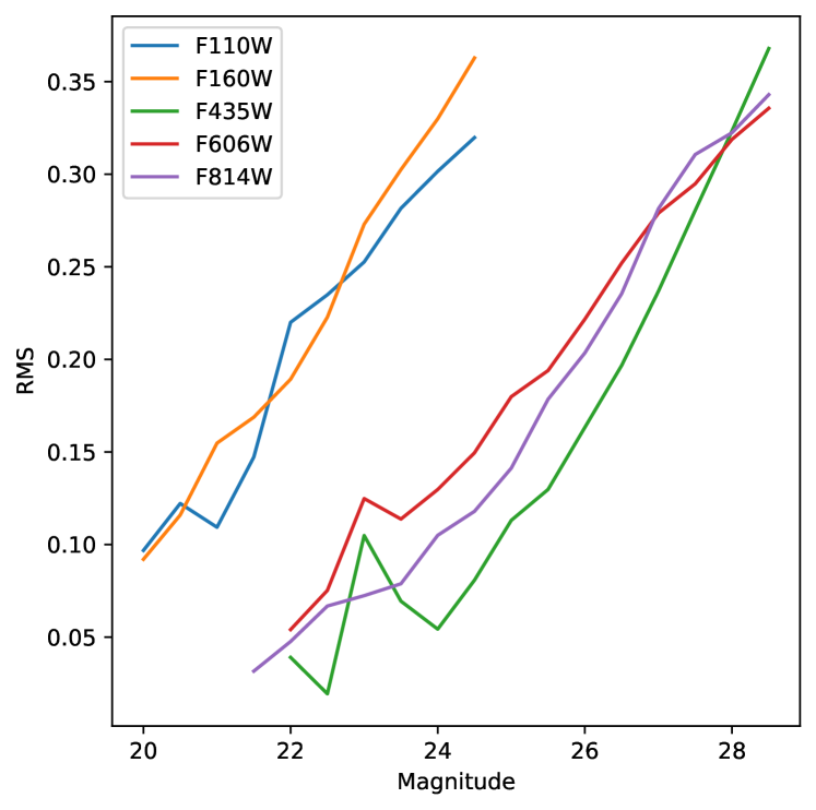
The rms errors (RMSE) on the ASTs’ magnitudes are shown in Figure 1. Errors in both the F110W and F160W filters are 0.1 at the bright end and 0.275 at the faint end.
We created an initial sample of red supergiant candidates using only the HST data through the use of PARSEC evolutionary tracks and isochrones. We used the stellar evolution models (Bressan et al., 2012, 2013; Chen et al., 2014; Tang et al., 2014) and computed isochrones using the collaborative CMD 3.3 input form (http://stev.oapd.inaf.it/cgi-bin/cmd, Bressan et al. (2012, 2013); Chen et al. (2014, 2015); Tang et al. (2014); Marigo et al. (2017); Pastorelli et al. (2019)). These references are for all the information that went into the isochrone calculation, all of which can also be found on the CMD input form. The only settings changed were the age range, which we set to .1-40 Myr (in 100,000 yr increments), and the filter set. This form creates isochrones with magnitudes in a specified filter set, so we created isochrones for both the HST/WFC3 and Spitzer filter sets. To correct for reddening, we add the distance modulus of 29.4 to the magnitudes in every filter, and then we add the respective galactic extinction of the filter (Schlafly & Finkbeiner, 2011).
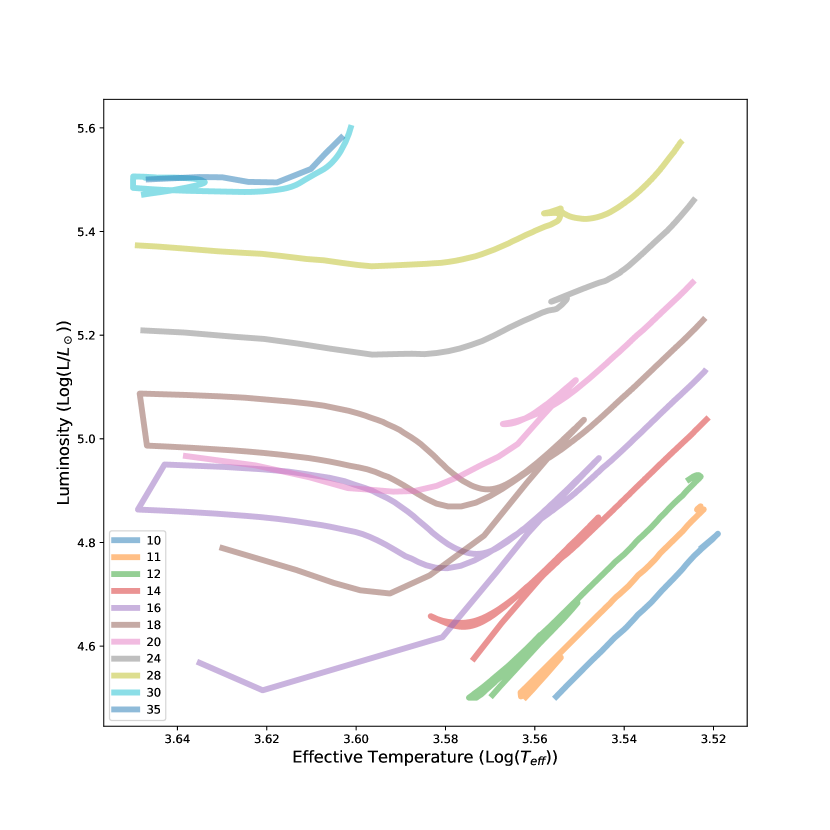
Model RSGs have effective temperatures of 3400-4300K, or Log() of 3.53-3.63 (Levesque, 2017). Figure 2 shows evolutionary tracks of 10-35 stars entering this temperature range with luminosities of . AGB and Super-AGB stars have initial masses of 8-9 so we avoid contamination from these stars by isolating tracks of stars with an initial mass 10. Applying the effective temperature, luminosity, and mass limits to the evolutionary models shows us that stars between the ages of 5.2 Myr and 26.3 Myr enter the space defined by our limits. These limits also give us a cap on the initial masses of these stars, making the mass range 10-35 (see Figure 2).
We then take the age range determined from the evolutionary tracks and employ the isochrones for stars in that range. Figure 3 shows IR CMDs of F110W-F160W vs F160W as two-dimensional histograms. The CMD points represent our data after the processing and filtering steps described above. Layered on top of the CMD are the isochrones of different ages along with model foreground stars from TRILEGAL (Vanhollebeke et al., 2009; Girardi & Marigo, 2007).
The input parameters for the TRILEGAL models follow the formulas in Table 1 of Pieres et al. (2020) and are laid out below:
-
•
Dust: Av mag (from the Schlegel maps, Schlegel et al. (1998)), scale height = 110 pc
-
•
Thin disk: exactly the same parameters as in the table
-
•
Thick disk: surface density = 0.0010 , scale length = 2913 pc, scale height = 800 pc (these were values previous to the recalibration done in Pieres et al. (2020))
-
•
Halo: a single power-law (and not two power laws as in Pieres et al. (2020)) with local density = 0.0001 , effective radius = 2698.93 pc, oblateness = 0.62, exponent = 2.75.
These values are the result of a recalibration with SDSS and 2MASS photometry mentioned in Girardi et al. (2012); however, the recalibration is a minor change with respect to the original calibration well documented in the original paper at Girardi et al. (2005).
The isochrones of 8-30 Myr stars show RSGs around an F110W-F160W color of 1. The isochrones and TRILEGAL foreground models allow us to make the following criteria that we can apply to our sample to avoid most of the foreground stars and eliminate unlikely RSGs; the cuts are shown in Figure 3:
-
1.
17.4 F160W 21.8
-
2.
-26.5(F110W-F160W)44.75F160W(F110W-F160W)29.2
-
3.
F110W - F160W 1.3
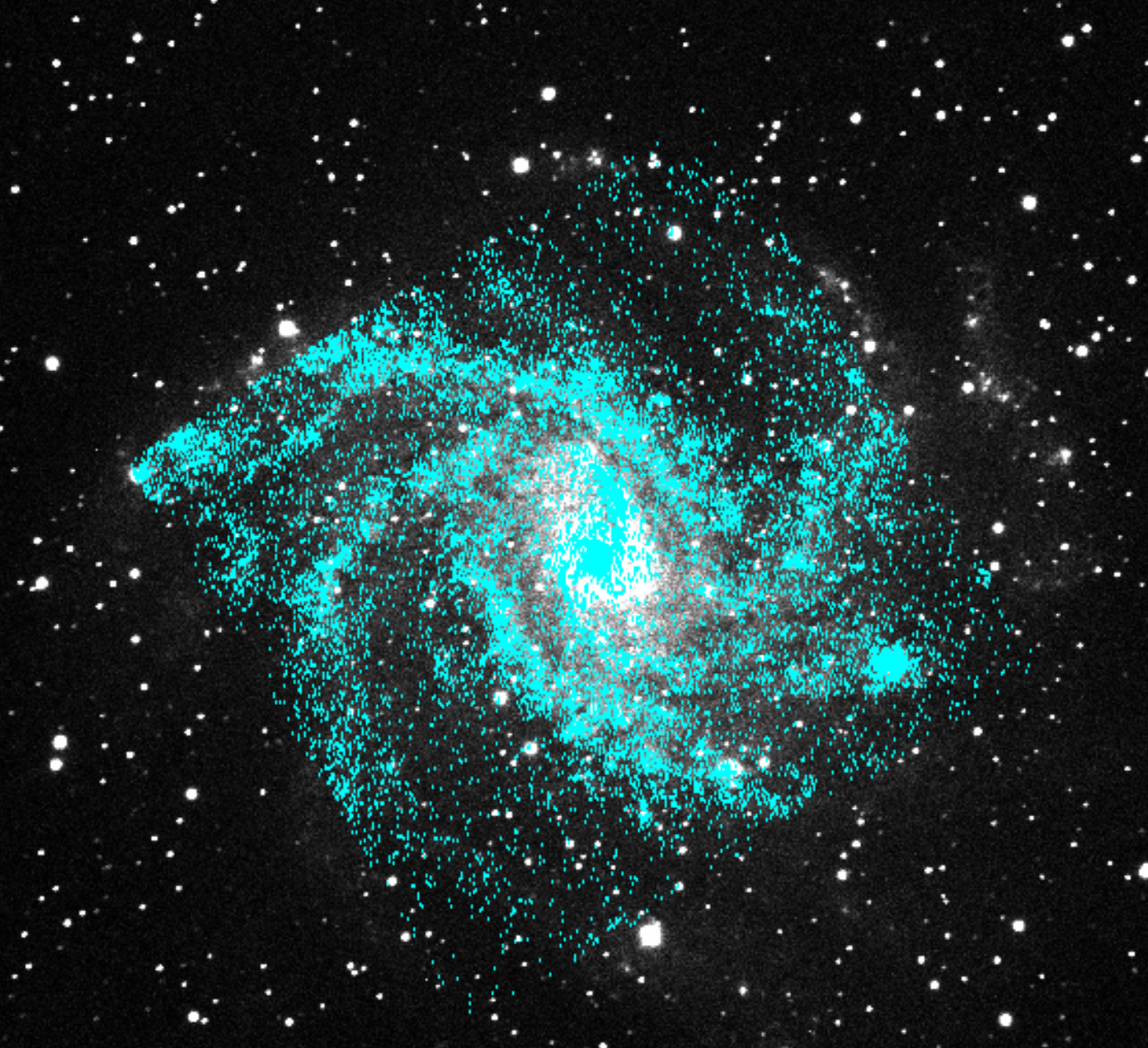
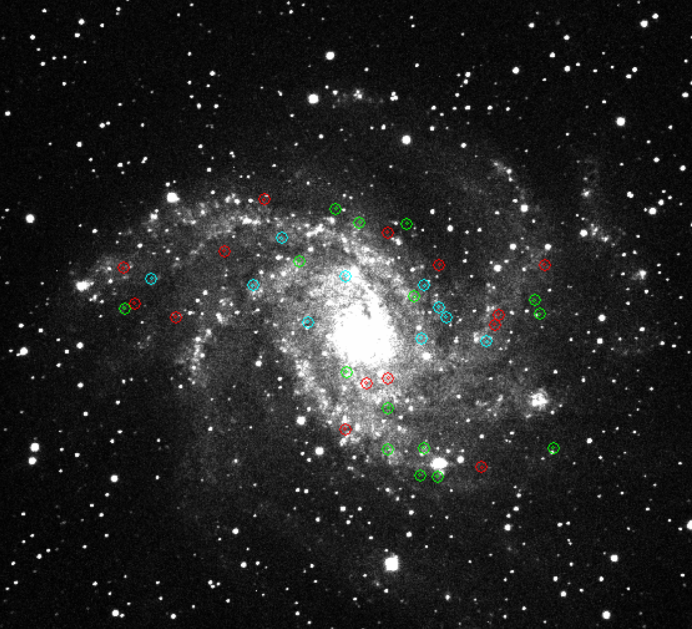
This produced a sample of 17,865 stars which we will refer to as the ’HST-only’ sample. The positions and magnitudes of these stars are provided in Table 2. Figure 4 shows our large HST-only sample mapped onto an image of NGC 6946. The positions of these stars line up very well with the spiral arms of the galaxy, which is expected when looking for young RSGs. To focus our sample and find an optimal set of the top candidates for follow-up study, we use additional information from Spitzer.
2.2 Spitzer Photometry
We supplemented our HST photometry with Spitzer bands using the catalog from Khan (2017). The photometry was taken with the 3.6, 4.5, 5.8, 8 m filters on the Infrared Array Camera (IRAC; Fazio et al. (2004)) on board the Spitzer Space Telescope (Werner et al., 2004). RSGs are bright in the Spitzer bands such as 3.6m and separate from other stars in some regions of color space (Bonanos et al., 2009).
We cross-correlated the Spitzer and HST photometry catalogs to ensure the same source was being detected in each catalog at the same location. Red supergiants are typically bright at mid-infrared wavelengths (Messineo et al., 2012). We therefore used the available Spitzer point-source catalog for NGC 6946 to find stars in our HST catalog with bright mid-infrared counterparts. Because the Spitzer resolution is much coarser than the resolution of HST, this matching was not straightforward. The original Spitzer catalog contained 15,815 sources but covered an area larger than our HST catalog did. After eliminating sources outside of our HST coverage area we have 7918 total Spitzer sources. We expect the majority of these to be AGB or RGB stars, which are far more numerous than more massive RSGs or background galaxies.
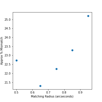
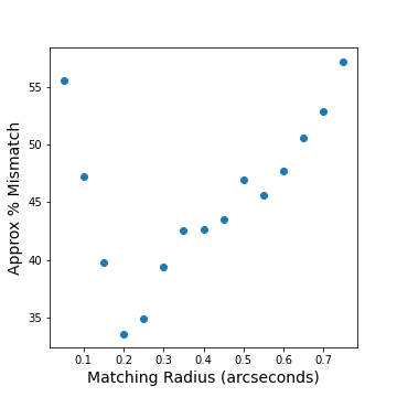
We estimated the best matching radius by identifying the radius with the lowest fraction of spurious matches to real matches. To address the simplest case, we started by limiting the cross-correlation to one-to-one matches. We tested radii ranging from 2 to 100 pixels on our HST reference image, where 1 pixel is 0.”05. We evaluated the rate of spurious matches for each radius by shifting the Spitzer coordinates by 8” and rerunning the matching procedure, such that all ’matches’ in the shifted case should be spurious. Figure 5 shows the fraction of spurious sources as a function of matching radius. There were differences in matching success depending on the density of surrounding sources. We determined an optimal matching radius of 13 pixels (corresponding to 0”.65 at 0”.05pixel) for candidates with only one HST source and one Spitzer source within the radius. This resulted in a 21.5% mismatch rate. There were no locations with multiple Spitzer sources within 0”.65. 385 paired HST and Spitzer sources were found at this 0”.65 radius and became our primary sample of RSG candidates.
While 0”.65 was found to be optimal for one-to-one matches between catalogs, in more crowded regions of the HST images, a 0”.65 search radius matched more than one HST source to some Spitzer sources. Therefore, we determined a separate limiting radius for sources with more than one match within the initial 0”.65 search. We optimized this radius by finding the lowest fraction of spurious to real matches within only these crowded regions. For candidates with multiple HST sources within 0”.65 of a Spitzer source, a smaller radius of 4 pixels (0”.2) was optimal for cross-correlation in a crowded space. If there were still multiple HST sources within this 0”.2 radius around a Spitzer source, the closest HST source was matched. Additionally, if there were multiple HST sources within 0”.65 but none within 0”.2, the closest HST source was matched to the Spitzer source. The technique of using a 0”.2 matching radius and taking the closest match in multiple-match cases had a higher mismatch rate of about 30%. The secondary radius technique resulted in 124 paired sources.
To obtain the highest quality sample of RSG candidates, we focus on our primary ’single’ match sample of 385. The secondary sample of 124 candidates is included in the tables and a figure, however we keep our analysis focused on the former sample. Both samples are put through selection criteria laid out in the rest of this section. The rmse on the Spitzer source positions is 0”.327 R.A. and 0”.242 decl.
2.3 Multiwavelength Culling of the Sample
We make additional cuts using Spitzer filters to narrow down to the most likely RSG candidates, based on existing studies of the SEDs of RSGs. We use a mix of selection criteria from Britavskiy et al. (2014), including the F110W - [3.6] 1 cut, which they also use to select for RSGs, and from the isochrones as described above. The criteria in Britavskiy et al. (2014); based on work from Bonanos et al. (2009)) used the J filter but we substituted the overlapping F110W filter.
The first three criteria below are mentioned above while the latter two are from Britavskiy et al. (2014).
-
1.
17.4 F160W 21.8
-
2.
-26.5(F110W-F160W)44.75F160W(F110W-F160W)29.2
-
3.
F110W - F160W 1.3
-
4.
F110W - [3.6] 1
-
5.
0
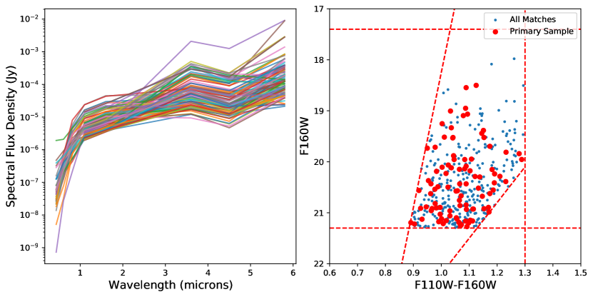
After combining all criteria and applying them to the 385 possible candidates, 24.4% of the candidates remain, which leaves us with 94 RSG candidates in the primary sample. We expect roughly 20 mismatches. A potential explanation for so few candidates passing these cuts is that we initially found many background galaxies. These galaxies will not have the colors we are selecting for and have now been removed from the sample. These same cuts were also applied to the secondary sample of 124 candidates and reduced the sample to 43 candidates.
We plot the candidates’ SEDs using our optical-mid-IR photometry in Figure 6. This is used to check for relative uniformity between the SEDs of our candidates. We converted HST and Spitzer magnitudes into flux values using the zero magnitude flux values () for HST from the SVO Filter Profile Service (Rodrigo et al. (2012); Rodrigo & Solano (2020); 4197.72, 3250.63, 2421.40, 1702.00, and 1132.88 for the F435W, F606W, F814W, F110W, and F160W filters, respectively) and used the IRAC Instrument Handbook (IRAC, 2020a, b) to get the values for Spitzer (280.9, 179.7, and 115 for the 3.6, 4.5, 5.6 micron filters, respectively).
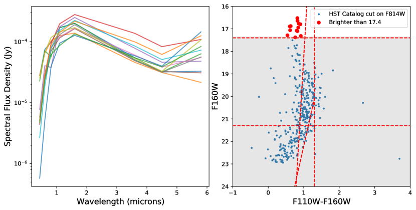
The SEDs in Figure 6 show excess flux toward the mid-IR associated with dust-enshrouded RSG stars. There is an example in Figure 7 showing SEDs of stars brighter than F160W magnitude 17.4. These stars show a peak flux density of 1.6m, a much different shape than our primary sample SEDs. The criteria adopted to identify RSGs are not perfect, so some stars shown in the SED could be foreground stars and some stars eliminated from the sample could be RSGs.
A compilation of all the magnitudes for each RSG candidate is shown in Table 3. The first column is a unique identifier for each RSG candidate. The identifier is the index of the star in the Spitzer data. Columns 2, 3, 4 and 5 give the R.A. and decl. for HST and Spitzer. Columns 6, 7, 8, 9, and 10 have the magnitudes of the HST filters F435W, F606W, F814W, F110W, and F160W respectively. Columns 11, 12, and 13 have the magnitudes of the Spitzer 3.6m, 4.5m, and 5.8m filters. Below we discuss other potential contaminants to this sample, which results in many of them being flagged as less likely candidates in Table LABEL:tab:MATCH_results (described in the introduction to Section 4).
Pairing HST and Spitzer sources resulted in a substantial decrease in the size of our viable sample. The much higher resolution of HST helps produce a clean sample of individual stars while Spitzer helps to identify bright red stars in its NIR filters. Because of the additional information from Spitzer, we are most confident in labeling the primary and secondary samples as our possible RSG candidates.
We calculated the approximate fraction of RSGs in NGC 6946 represented in our sample by estimating how many red supergiants we expect to see in the galaxy based on the star formation rate. Using a star formation rate of 3.2yr-1 (Jarrett et al., 2012) over a period of 30 Myr, we expect roughly 96 million solar masses to be formed. Assuming a Kroupa IMF and integrating between our mass range of 10-35 we estimate 400,000 RSGs forming in NGC6946 over a 30 Myr period. From the PARSEC evolutionary tracks the lifetime of RSGs is 600,000 yr, or about 2% of these 30 Myr. Thus, we may expect 8000 RSGs to be present in the whole galaxy. Therefore, our HST-only sample likely has about 50% contamination; however, our small primary sample, which has very few stars with significantly more vetting, is likely to be much cleaner. The size of our primary sample is not surprising given the high degree of crowding of the Spitzer data. High-resolution mid-IR photometry, perhaps from future observations with the James Webb Space Telescope, will likely yield many more high-quality RSG candidates.
2.4 Contamination
We further culled our sample of RSG candidates by visual inspection and comparison with Gaia. Using the Gaia Single Source service (Prusti et al., 2016; Brown et al., 2018), we were able to visually inspect each location and compare the R.A. and decl. of the HST and Spitzer detections, and determine likely mismatches as well as foreground stars. Each candidate had different coordinates for the HST and Spitzer detections. With these visual inspections, we found 19 locations where a much brighter nearby star would more likely be the Spitzer detection than the fainter HST source from the sample. This was slightly below the number of mismatches we expected. These candidates were labeled as mismatches between the HST and Spitzer catalogs. Furthermore, another 21 candidates had measured proper motions in Gaia, and therefore are likely foreground stars. Removing these likely mismatches and foreground stars brings us to 54 RSG candidates. The removed candidates are labeled in Table LABEL:tab:MATCH_results with the ”M” and ”F” flags for mismatches and foreground. The secondary sample was reduced to 11 candidates after removing the mismatches and foreground stars. We found 22 mismatches, and 10 foreground stars were identified in the secondary sample. We expected 13 mismatches from this sample.
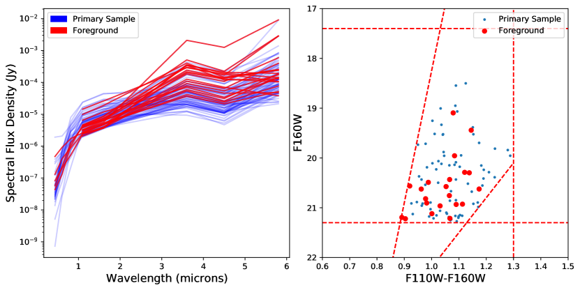
Identifying some very likely foreground stars in our sample allowed us to plot their SEDs to compare against the rest of the sample. Figure 8 shows SEDs color coded according to the group they belong to. Our primary sample is in blue and the identified foreground stars in red. We found that the blending of multiple stars could be responsible for SEDs peaking at 3.6m. The vast majority of these SEDs belonged to mismatched or foreground stars. The Spitzer resolution is much lower than HST, so multiple resolved stars in the HST catalog may be only a single, erroneously bright, Spitzer detection.
In addition to contamination from the foreground, there could be bright red stars in NGC 6946 that are not RSGs, such as AGB stars. Although our luminosity selection is brightward of the evolutionary pathways of nearly all low-mass stars, AGB stars entering our defined temperature and luminosity space is still a major concern. The possible AGB contaminants are labeled as such with the ”C” flag in Table LABEL:tab:MATCH_results identified by their cooler temperatures and lower luminosities. The candidate locations now labeled possible AGB contaminants all returned star formation within our accepted age ranges making them still viable RSG candidates as well. A figure showing these possible contaminants compared to our selection criteria and results is discussed later in Section 4.1.1.
3 Analysis
The overall goals of our analysis were to find a reliable set of RSG candidates in NGC 6946, constrain their ages, and compare their ages and photometric properties to stellar evolution models. In the following subsections, we will first discuss using MATCH to determine ages, and then the existing models we will use to compare against our results.
3.1 Constraining RSG Candidate Ages
Previous work has shown that some of the young stars within a 50 pc radius from a point are likely to be coeval, allowing the neighboring stars to be used for age dating (Gogarten et al., 2009; Williams et al., 2014). This is especially true for younger stars that have less time to travel away from their original population. From Bastian & Goodwin (2006), stars formed from a common event maintain a spatial relationship at distances up to 100pc for about 100 Myr. Applying the initial velocity dispersion, usually a few km-s, the stars bound to escape the cluster are still associated with the cluster for 15-45 Myr. It is therefore likely that most young stars in a 50 pc area have coevolved, although not all stars. We take multiple steps to reduce possible contamination within our targeted location including foreground stars as described above and the use of background CMDs, which we discuss later in this section. Therefore, we can infer the likely ages of the RSGs by analyzing the surrounding stellar population. To determine an age distribution for each of the RSG candidates we used MATCH (Dolphin, 2002, 2013). This program models the CMDs to infer star formation history (SFH) for that stellar population. The resulting SFH from MATCH includes a distribution of ages, metallicities, and uncertainties on these values. We use the distribution of ages as a proxy for the probability that the RSG candidate is of a certain age.
MATCH applies two types of extinction to the model CMDs when fitting the data. These are called which represents the differential extinction within the region being measured and which accounts for the uniform foreground extinction in the region. These and values were solved for by inputting a range of values and MATCH would choose the most likely value corresponding to the best fit. We tested fits to the data with a grid of possible , and to determine the best combination for each region. To determine the value we calculated the best fit to the observed CMD, testing values greater than 0.8 (slightly below the foreground value of Schlegel et al. (1998)) in 0.05 increments. We also supplied MATCH with some restrictions on metallicity to limit the parameter space of the fitting. Cedrés et al. (2012) found an NGC 6946 metallicity that is approximately solar. A range of metallicities from [Fe/H] was used as the MATCH input. The most consistent metallicity results from MATCH are [Fe/H] = , which is also consistent with the metallicity of the models used in this paper, described later in Section 3.2. Finally, we applied background CMDs to isolate the unique population associated with the positions of the RSG candidates. These background CMDs are taken from an annulus extending from 50 pc to 1 kpc around each source. We then weighed the contamination CMDs to the area of the original radius. This contamination CMD also helps to correct for foreground issues as these stars are also evenly distributed across the face of the galaxy. Moreover, the main sequence of young stars in NGC6946 is bluer than the foreground stellar sequence.
Following the technique used by previous work in determining ages using MATCH age distributions (Jennings et al., 2012; Williams et al., 2019), we find the median age of the young stars in the best fit for the sample at each location. We then assign that as the most likely age of the RSG candidate. We restrict the maximum age to 30 Myr because the models (described in Section 3.2.1) show that the maximum age of RSGs is 30 Myr. Thus, older ages present are not likely to have stars remaining that are massive enough to become RSGs. If the location around an RSG candidate does not show significant star formation at an age 30 Myr or younger, we assign an age of zero. The uncertainty on the age is calculated by resampling the age distribution output, applying draws from the measured uncertainties, recalculating the best-fit age, and analyzing the distribution of resulting best-fit ages. More details on this technique of estimating age uncertainties can be found in Williams et al. (2018, 2019). We tested the effect of offsetting the position of the RSG candidate to see how that would change the number of stars in the neighborhood of the candidate. We tested an offset of 0”.25 and found that the sample of stars around each candidate typically changed by 4%. We reran these offset locations through MATCH and found no change in the best-fit ages.
To create the input CMD for MATCH, all HST sources in a 50 pc radius around each candidate location were put into separate catalogs, excluding the actual RSG candidate. Because the infrared has poor sensitivity to the upper main sequence stars, which are blue, and because crowding limits the depth of the IR imaging, we were only able to constrain the population ages for regions that had complimentary optical HST imaging. Since there is only optical coverage of 2% of our HST-only sample, this subset could produce some bias in the age analysis. However, because the optical coverage is not focused on any particular galaxy feature (e.g., the center or a single star-forming region), such a bias should be minimal.
There are parts of NGC 6946 that we do not have F814W coverage for. We analyzed 15 stars from the primary sample using the F435W and F606W filter combination. The remaining 32 stars from the primary sample and the entire secondary sample were analyzed using the F606W and F814W combination. We found seven locations from the primary sample, that were not already removed, which had HST optical coverage in only one band. This coverage was insufficient to be analyzed using MATCH. Thus, although we did not have optical coverage over the entire galaxy, the areas with insufficient data only resulted in seven fewer age measurements. MATCH outputs an SFH for each value attempted. We calculate the most likely age using the SFH from the best fit . In Figure 9 we show an example of one CMD fitted by MATCH, its output SFR, and uncertainties on that SFR. The figure shows the cumulative stellar mass with a most likely age, the best value, and the CMD fitted by MATCH with both real magnitudes and background fake magnitudes. The figure also contains a rerun of the MATCH output to better constrain the uncertainties on the SFH. MATCH takes into account both the photometric uncertainties when fitting the models. In short, MATCH determines the photometric uncertainties and completeness for each color and magnitude bin from the AST results, and it applies these measurements to the models during the fitting. Then, during the Monte Carlo error analysis, both the uncertainties and the sampling are taken into account. A large number of model realizations are created using photometry, background CMDs, and artificial stars. Then the SFH is recalculated for each realization. The variance of these SFHs then provides the uncertainty on the best-fitting SFH assigned to each location (Dolphin, 2012, 2013).
The SFHs of these regions are consistent with the existence of an RSG candidate in our selection region. We tested this consistency by generating many model CMDs in the IR bands using a sample of our SFHs and calculating the fraction of draws from the model that contained at least one RSG candidate. All SFH models had at least 25% probability of producing a star with IR color and magnitude inside of our selection region, and 50% had at least 95% probability of producing such a star.
3.2 RSG evolutionary models
In this section, we briefly describe the models used to compare to our age measurements and use the evolutionary tracks and isochrones to test their consistency with our age measurements.
3.2.1 PARSEC and Geneva
Two widely used sets of single stellar evolution models are from the PARSEC and Geneva (Ekström et al., 2012) groups. We compare our age results against each of these sets below.
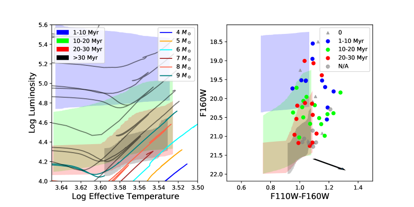
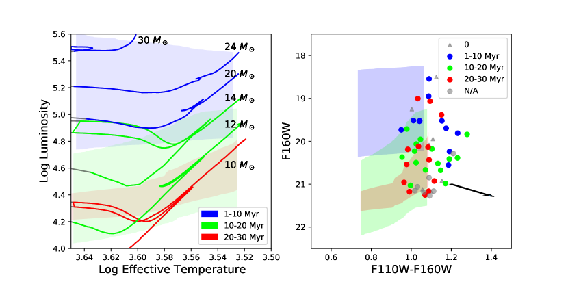
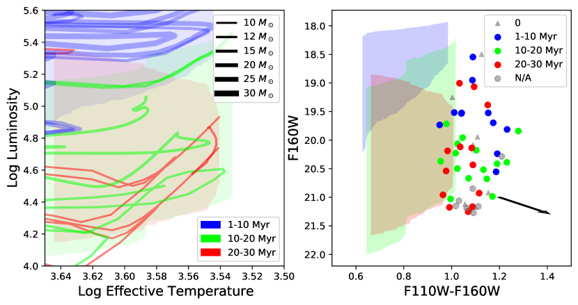
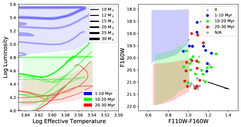
Figure 10 contains a plot that shows the evolutionary tracks of stars with a few different masses entering our defined RSG space on the left panels. The colored regions indicate the area covered by our age ranges of interest on both the track plot and the CMD plot. These areas were determined from the magnitude values given in the isochrones by first removing points that do not pass our luminosity, effective temperature, magnitude, and color limits. We then generated a polygon to cover the remaining points. Thus, the polygons in the CMD correspond to the polygons of the same color in luminosity and temperature space in the model isochrones and evolutionary tracks.
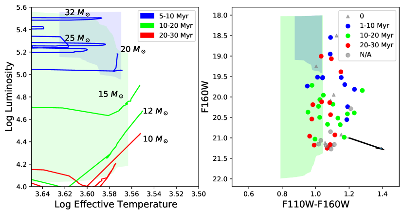
We applied the same process to the Geneva (Ekström et al., 2012) tracks and isochrones. The Geneva model has fewer data points in their model grids. We use isochrone files with a log age of 6.75-7.6 in increments of 0.05 log age. We use tracks from stars with a mass of 10, 12, 15, 20, 25, and 32 solar masses.
3.2.2 BPASS
The BPASS models (Eldridge et al., 2017; Stanway & Eldridge, 2018) are the final set of models we compared against our results. The BPASS models have both binary and secular options. As a result, the process of creating the figures containing the data from BPASS was quite different from both the previous models. Instead of separate files for tracks and isochrones, BPASS comes in one large suite of stellar models, including a couple thousand individual binary models. These models were labeled by their metallicity, mass of the initially less massive star (treated as primary in subsequent evolution), mass of the remnant after death of the initially more massive star, and the log of the binary period after remnant formation. For simplicity, we only considered the models with a solar metallicity and 10, 12, 15, 20, 25 and 30 solar masses, leaving a grid of close to 200 models for each mass for comparison against our RSG observations. Instead of plotting all 200 for each mass, in Figure 11 we plot a file with a relatively high luminosity maximum for the mass, a file with a relatively low luminosity minimum, and then an average luminosity file. We found this technique captured the range of temperature and luminosities we would find with plotting all the files but is much easier to see. The resulting regions of temperature, as well as CMD space, for each age are plotted in Figure 11 using the same color coding as for the single-star PARSEC and Geneva models.
4 Results and Discussion
The results from MATCH are shown in Table LABEL:tab:MATCH_results. Column 1 has the unique identifier for each RSG candidate. Columns 2 and 3 contain the best fit and values. Column 4 has the best age result in Myr. Finally, column 5 contains a flag used to indicate the quality of the candidate as well as which sample the candidate belongs to. A means the candidate has shown only signs of being a quality candidate. B indicates the candidate is in a potential binary system, C means the star is a potential low-mass contaminant (AGB star), D means the candidate location was analyzed with the F435W and F606W filter combination, F means the star is a potential foreground star, M indicates the candidates that were our most likely mismatches, and IN means the location had insufficient coverage in the surrounding area to get an age estimate from MATCH. A flag of 1 means the candidate belongs to the primary sample comprised of only single matches between HST and Spitzer sources while 2 means the candidate belongs to the secondary sample of candidates that had multiple matches between HST and Spitzer sources.
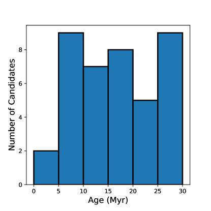
Figure 12 shows a histogram of the MATCH results with contamination CMDs. The figure shows nearly all candidates are older than 5 Myr, as one might expect given the small number of very massive stars produced by a standard initial mass function. We found seven RSG candidate locations showing no significant star formation Myr, which indicates that they are either not RSGs or have unusually high velocities that have moved away from their siblings. For example, these stars could be AGB or post-AGB contaminants that entered our sample. AGB stars are older than our age cap of 30 Myr and would receive an age value of zero from MATCH, as shown in Figure 10. These potential contaminants were excluded from the histogram in Figure 12
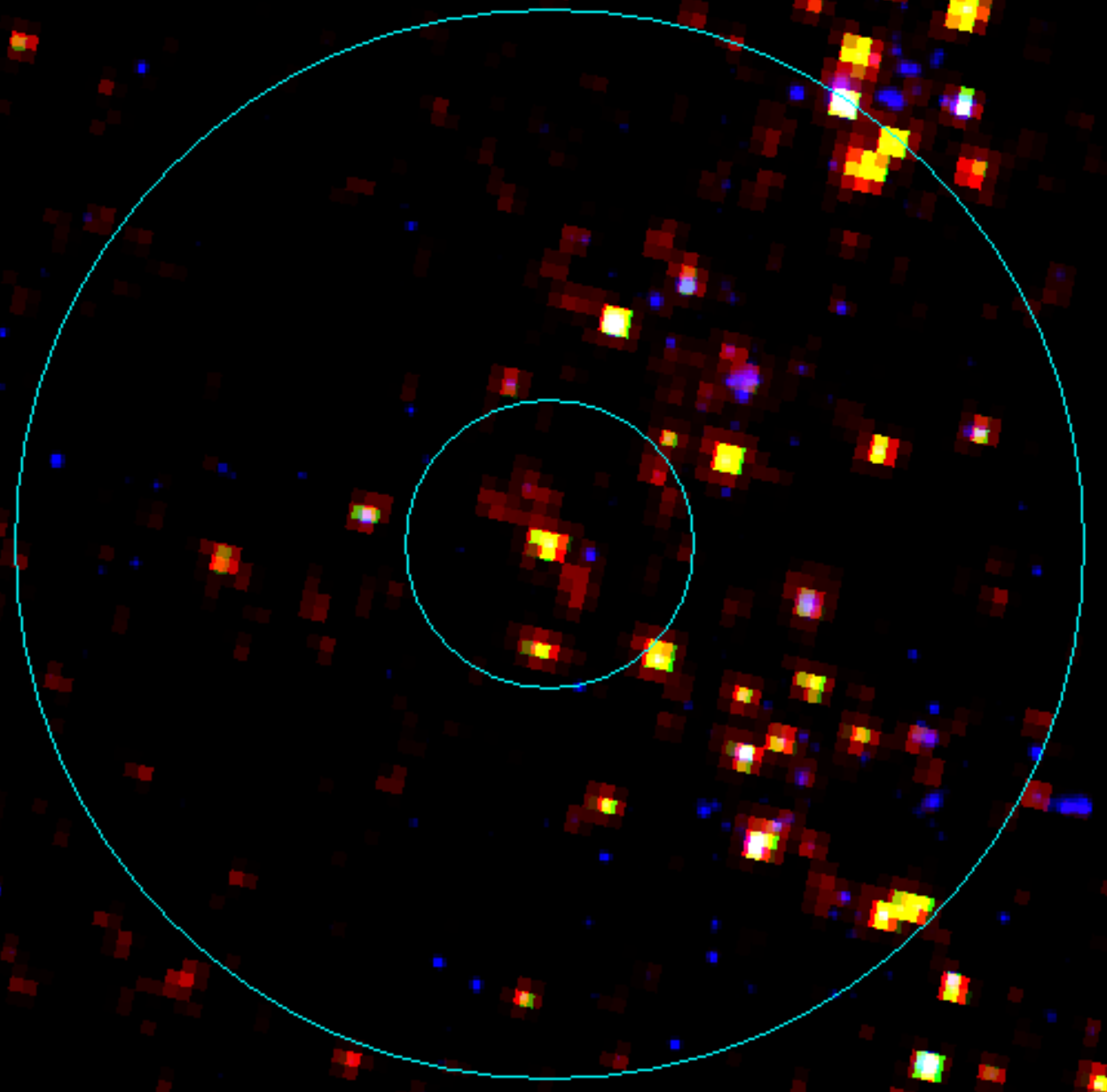
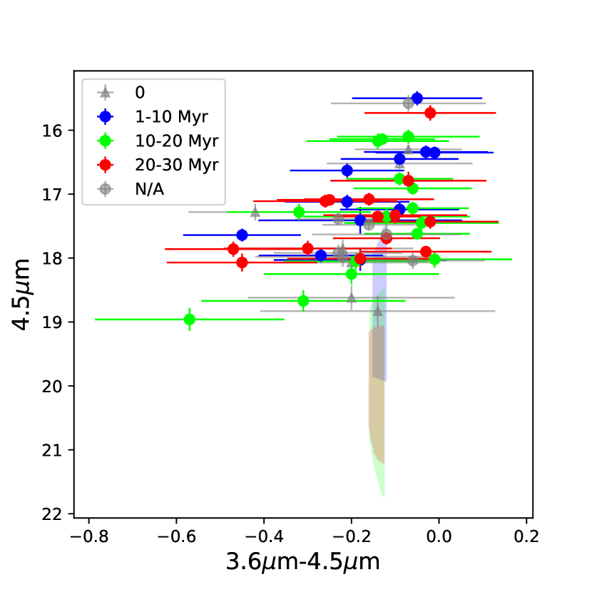
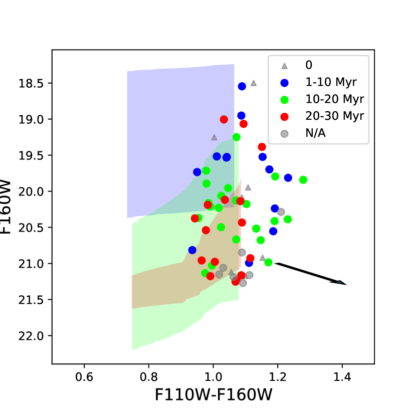
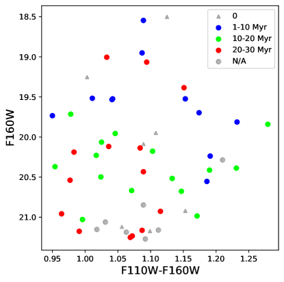
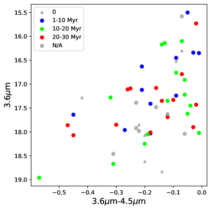
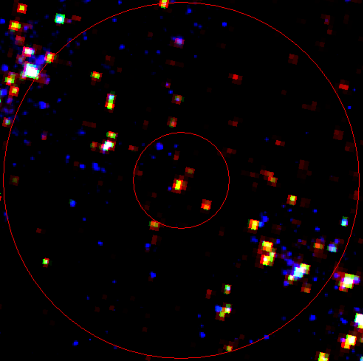
A pair of CMDs in the HST filters and Spitzer filters is shown in Figure 13 showing the 40 candidates plus the seven candidates returning an age of zero and seven candidates that did not have sufficient detected stars in the surrounding area to calculate an age. Figure 14 shows NGC 6946 overlaid with the locations of the RSG candidates color coded by age. Finally, we show close-up color images for some RSG candidates, in Figure 15. All of the primary sample candidates with an ’A’ flag will have images in the online journal as stated in Figure 16. These images use the F160W filter for red, F110W for green, and F606W for blue.
4.1 Comparing Our Measured Ages to Models
In this section we discuss the different models used to interpret our results and the techniques for doing so. We also discuss how AGB stars could show up in the models and what that means for our candidate selection. Without spectroscopy, we cannot measure a mass for these candidates, but in this section we use the models to provide mass estimates for the candidates that are most likely to be RSG stars.
4.1.1 PARSEC and Geneva
Figure 10 shows the red supergiant region of the evolutionary tracks from the PARSEC models along with the age range that corresponds with the stars that passed the cuts. On this plot we also show polygons of parameter space on the CMD color coded by the age bin. These polygons are the ranges of F160W and F110W-F160W allowed values from the PARSEC isochrones. In Figure 10, the panels on the right-hand side represent the models and the RSG candidates in the HST filters while the bottom panel on the left shows the models and candidates in Spitzer filters.
We also used the PARSEC models to investigate how AGB stars could potentially contaminate our sample. Figure 17 is a plot showing how AGB stars could intrude on our defined space. Lower-mass stars from 4-9 are plotted along with the original selection from the HST part of Figure 10. The luminosity minimum was lowered from 4.5 to 4.2. This extended the allowed region fainter than our RSG selection would allow. One important note to consider is that the 4-9 evolutionary tracks are all older than our 30 Myr maximum allowed age in the MATCH analysis.
Figure 18 shows the red supergiant portions of the Geneva models for direct comparison to PARSEC. There were no models in the 20-30 Myr age range with temperatures and luminosities that would place them in our photometry sample, so no red region is drawn on the CMD. The 10-20 Myr range dominated the entire color-magnitude region covered by our RSG candidates. By using multiple single-star evolution models we can show the discrepancies in the models in this phase of evolution. Between PARSEC and Geneva we show differences in the range of luminosity and temperature according to the age of RSGs.
4.1.2 BPASS
Figure 11 was created from the BPASS Binary and Secular models. These models are similar to the space of the CMD regions in the PARSEC models. Although, the regions in both the Binary and Secular models span a wider color space and are shifted slightly red compared to the PARSEC models. The binary models show that stars within the 20-30 Myr age range can be around a 19th mag in F160W. Before the BPASS binary model, the brightest stars in the 20-30 Myr age range from the results were not mirrored in the models. This provides evidence for the possibility of the three RSG candidates with age results between 20 and 30 Myr and an F160W magnitude between 19 and 19.5 as being in binary star systems. These candidates are labeled with the ’B’ flag in Table LABEL:tab:MATCH_results.
4.2 Predicting Mass
All of this information gathered from the models can help us predict the masses of the candidates. From the PARSEC isochrones, we can get a range of masses for each set of ages in the results. Model stars from the isochrones that pass all other cuts are allowed to be 5.4 Myr at the youngest and 26.3 at the oldest. Model stars with an age between 5.4 and 9.9 Myr will correspond to masses between 17.76 and 30.05, stars with an age between 10-19.9 Myr correspond to 11.19-17.77, and ages 20-26.3 Myr to 10-11.72, 10 being the lowest mass we were accepting values for.
Out of the 40 highest quality candidates, four of them fall within the 17.76-30.05 mass range, 15 fall within the 11.19-17.77 range, and five fall within the 10-11.72 range. For the secondary match sample and the same mass ranges we find zero candidates, seven candidates, and one candidate, respectively. Without spectroscopy, we are unable to verify our mass constraints on these individual stars. We hope to perform such spectroscopic verification in future work.
5 Conclusion
We gathered images of NGC 6946 in the F435W, F606W, F814W, F110W, and F160W HST filters and measured photometry using a PSF. DOLPHOT gave us quality metrics on our photometry which we used to make cuts to improve our catalogs. We applied several stellar evolutionary model sets to determine the color and luminosity space where RSG stars should appear in our photometry catalogs. After matching the HST catalog with a Spitzer catalog, analyzing multiwavelength SEDs, comparing to Gaia, and visually inspecting HST imgaging, we have generated a sample of stars likely to be RSGs in NGC 6946. Using MATCH we inferred ages for the candidates from their surrounding stellar populations, which we then compared to current evolutionary models and isochrones.
Our comparisons to evolutionary models suggest that RSGs can have a broader range magnitudes and color in the Spitzer bands than the models predict. The model magnitudes and colors of RSGs in Spitzer bands are very narrow, and the data shows a much broader and bluer range of colors. On the other hand, the model predictions in the HST IR bands more closely match those seen in the data. We found general agreement between the ages of the populations near the RSGs and the colors and luminosities predicted for RSGs at those ages.
Furthermore, the few cases that disagreed with the ages of single-star models were better matched with the ages of binary models, making them good binary RSG candidates. From the BPASS models we can see that binary systems are a possible explanation for some of the older candidates being much brighter than the models and the other stars within the same age group. Three out of the 40 primary candidates show this evidence for being strongly affected by binary evolution.
In the future, acquiring spectroscopy of the RSG candidates identified previously would allow us to compute mass values for these stars. With profound advances in astronomical imaging on the horizon (projects such as JWST, Nancy Grace Roman Space Telescope, LSST, and Thirty Meter Telescope), studying RSG stars is not only becoming easier but is also going to be a key to understanding more about supernovae and the stellar evolution process preceding the violent death.
Support for this work was provided by NASA through grant GO-15216 from the Space Telescope Science Institute, which is operated by the Associations of Universities for Research in Astronomy, Incorporated, under NASA contract NAS5-26555.
A special thank you to Emily Levesque and Kathryne Neugent for advising us on our RSG candidate selection process and to look out for AGB stars.
This work has made use of data from the European Space Agency (ESA) mission Gaia (https://www.cosmos.esa.int/gaia), processed by the Gaia Data Processing and Analysis Consortium (DPAC, https://www.cosmos.esa.int/web/gaia/dpac/consortium). Funding for the DPAC has been provided by national institutions, in particular the institutions participating in the Gaia Multilateral Agreement.
This research has made use of the NASA/IPAC Extragalactic Database (NED), which is funded by the National Aeronautics and Space Administration and operated by the California Institute of Technology.
This research has made use of the SVO Filter Profile Service (http://svo2.cab.inta-csic.es/theory/fps/) supported from the Spanish MINECO through grant AYA2017-84089
References
- Adams et al. (2017) Adams, S. M., Kochanek, C. S., Gerke, J. R., Stanek, K. Z., & Dai, X. 2017, MNRAS, 468, 4968, doi: 10.1093/mnras/stx816
- Anand et al. (2018) Anand, G. S., Rizzi, L., & Tully, R. B. 2018, The Astronomical Journal, 156, 105, doi: 10.3847/1538-3881/aad3b2
- Anderson & Soto (2013) Anderson, J. P., & Soto, M. 2013, A&A, 550, A69, doi: 10.1051/0004-6361/201220600
- Bastian & Goodwin (2006) Bastian, N., & Goodwin, S. P. 2006, MNRAS, 369, L9, doi: 10.1111/j.1745-3933.2006.00162.x
- Bonanos et al. (2009) Bonanos, A. Z., Massa, D. L., Sewilo, M., et al. 2009, AJ, 138, 1003, doi: 10.1088/0004-6256/138/4/1003
- Bressan et al. (2013) Bressan, A., Marigo, P., Girardi, L., Nanni, A., & Rubele, S. 2013, EPJ Web of Conferences, 43, 03001, doi: 10.1051/epjconf/20134303001
- Bressan et al. (2012) Bressan, A., Marigo, P., Girardi, L., et al. 2012, MNRAS, 427, 127, doi: 10.1111/j.1365-2966.2012.21948.x
- Britavskiy et al. (2014) Britavskiy, N. E., Bonanos, A. Z., Mehner, A., et al. 2014, A&A, 562, A75, doi: 10.1051/0004-6361/201322709
- Brown et al. (2018) Brown, A. G. A., Vallenari, A., Prusti, T., et al. 2018, Astronomy & Astrophysics, 616, A1, doi: 10.1051/0004-6361/201833051
- Cedrés et al. (2012) Cedrés, B., Cepa, J., Bongiovanni, Á., et al. 2012, A&A, 545, A43, doi: 10.1051/0004-6361/201219571
- Chen et al. (2015) Chen, Y., Bressan, A., Girardi, L., et al. 2015, MNRAS, 452, 1068, doi: 10.1093/mnras/stv1281
- Chen et al. (2014) Chen, Y., Girardi, L., Bressan, A., et al. 2014, Monthly Notices of the Royal Astronomical Society, 444, 2525, doi: 10.1093/mnras/stu1605
- Coughlin et al. (2018) Coughlin, E. R., Quataert, E., & Ro, S. 2018, ApJ, 863, 158, doi: 10.3847/1538-4357/aad198
- Dolphin (2016) Dolphin, A. 2016, DOLPHOT: Stellar photometry. http://ascl.net/1608.013
- Dolphin (2000) Dolphin, A. E. 2000, PASP, 112, 1383, doi: 10.1086/316630
- Dolphin (2002) —. 2002, MNRAS, 332, 91, doi: 10.1046/j.1365-8711.2002.05271.x
- Dolphin (2012) —. 2012, ApJ, 751, 60, doi: 10.1088/0004-637X/751/1/60
- Dolphin (2013) —. 2013, ApJ, 775, 76, doi: 10.1088/0004-637X/775/1/76
- Ekström et al. (2012) Ekström, S., Georgy, C., Eggenberger, P., et al. 2012, A&A, 537, A146, doi: 10.1051/0004-6361/201117751
- Eldridge et al. (2017) Eldridge, J. J., Stanway, E. R., Xiao, L., et al. 2017, Publications of the Astronomical Society of Australia, 34, e058, doi: 10.1017/pasa.2017.51
- Eldridge & Xiao (2019) Eldridge, J. J., & Xiao, L. 2019, Monthly Notices of the Royal Astronomical Society: Letters, 485, L58, doi: 10.1093/mnrasl/slz030
- Fazio et al. (2004) Fazio, G. G., Hora, J. L., Allen, L. E., et al. 2004, ApJS, 154, 10, doi: 10.1086/422843
- Girardi et al. (2005) Girardi, L., Groenewegen, M. A. T., Hatziminaoglou, E., & da Costa, L. 2005, A&A, 436, 895, doi: 10.1051/0004-6361:20042352
- Girardi & Marigo (2007) Girardi, L., & Marigo, P. 2007, in Astronomical Society of the Pacific Conference Series, Vol. 378, Why Galaxies Care About AGB Stars: Their Importance as Actors and Probes, ed. F. Kerschbaum, C. Charbonnel, & R. F. Wing, 20. https://arxiv.org/abs/astro-ph/0701533
- Girardi et al. (2012) Girardi, L., Barbieri, M., Groenewegen, M. A. T., et al. 2012, in Astrophysics and Space Science Proceedings, Vol. 26, Red Giants as Probes of the Structure and Evolution of the Milky Way, 165, doi: 10.1007/978-3-642-18418-5_17
- Gogarten et al. (2009) Gogarten, S. M., Dalcanton, J. J., Murphy, J. W., et al. 2009, ApJ, 703, 300, doi: 10.1088/0004-637X/703/1/300
- Hack et al. (2012) Hack, W. J., Dencheva, N., Fruchter, A. S., et al. 2012, in American Astronomical Society Meeting Abstracts, Vol. 220, American Astronomical Society Meeting Abstracts #220, 135.15
- Higgins & Vink (2019) Higgins, E. R., & Vink, J. S. 2019, Astronomy & Astrophysics, 622, A50, doi: 10.1051/0004-6361/201834123
- IRAC (2020a) IRAC. 2020a, IRAC Instrument Handbook. https://irsa.ipac.caltech.edu/data/SPITZER/docs/irac/iracinstrumenthandbook/6/
- IRAC (2020b) —. 2020b, IRAC Instrument Handbook. https://irsa.ipac.caltech.edu/data/SPITZER/docs/irac/iracinstrumenthandbook/17/#_Toc410728305
- Jarrett et al. (2012) Jarrett, T. H., Masci, F., Tsai, C. W., et al. 2012, The Astronomical Journal, 145, 6, doi: 10.1088/0004-6256/145/1/6
- Jennings et al. (2012) Jennings, Z. G., Williams, B. F., Murphy, J. W., et al. 2012, The Astrophysical Journal, 761, 26, doi: 10.1088/0004-637x/761/1/26
- Kennicutt et al. (2003) Kennicutt, Robert C., J., Armus, L., Bendo, G., et al. 2003, PASP, 115, 928, doi: 10.1086/376941
- Khan (2017) Khan, R. 2017, The Astrophysical Journal Supplement Series, 228, 5, doi: 10.3847/1538-4365/228/1/5
- Koplitz et al. (2021) Koplitz, B., Johnson, J., Williams, B. F., et al. 2021, The Masses of Supernova Remnant Progenitors in NGC 6946. https://arxiv.org/abs/2104.11118
- Krist et al. (2011) Krist, J. E., Hook, R. N., & Stoehr, F. 2011, in Optical Modeling and Performance Predictions V, ed. M. A. Kahan, Vol. 8127, International Society for Optics and Photonics (SPIE), 166 – 181, doi: 10.1117/12.892762
- Levesque (2017) Levesque, E. M. 2017, Astrophysics of Red Supergiants (IOP Publishing), doi: 10.1088/978-0-7503-1329-2
- Marigo et al. (2017) Marigo, P., Girardi, L., Bressan, A., et al. 2017, ApJ, 835, 77, doi: 10.3847/1538-4357/835/1/77
- Massey et al. (2017) Massey, P., Levesque, E., Neugent, K., et al. 2017, in IAU Symposium, Vol. 329, The Lives and Death-Throes of Massive Stars, ed. J. J. Eldridge, J. C. Bray, L. A. S. McClelland, & L. Xiao, 161–165, doi: 10.1017/S1743921317002642
- Messineo et al. (2012) Messineo, M., Menten, K. M., Churchwell, E., & Habing, H. 2012, A&A, 537, A10, doi: 10.1051/0004-6361/201117772
- Pastorelli et al. (2019) Pastorelli, G., Marigo, P., Girardi, L., et al. 2019, MNRAS, 485, 5666, doi: 10.1093/mnras/stz725
- Pieres et al. (2020) Pieres, A., Girardi, L., Balbinot, E., et al. 2020, Monthly Notices of the Royal Astronomical Society, 497, 1547, doi: 10.1093/mnras/staa1980
- Prusti et al. (2016) Prusti, T., de Bruijne, J. H. J., Brown, A. G. A., et al. 2016, Astronomy & Astrophysics, 595, A1, doi: 10.1051/0004-6361/201629272
- Raithel et al. (2018) Raithel, C. A., Sukhbold, T., & Özel, F. 2018, ApJ, 856, 35, doi: 10.3847/1538-4357/aab09b
- Rodrigo & Solano (2020) Rodrigo, C., & Solano, E. 2020, in Contributions to the XIV.0 Scientific Meeting (virtual) of the Spanish Astronomical Society, 182
- Rodrigo et al. (2012) Rodrigo, C., Solano, E., & Bayo, A. 2012, SVO Filter Profile Service Version 1.0, IVOA Working Draft 15 October 2012, doi: 10.5479/ADS/bib/2012ivoa.rept.1015R
- Rui et al. (2019) Rui, L., Wang, X., Mo, J., et al. 2019, MNRAS, 485, 1990, doi: 10.1093/mnras/stz503
- Schlafly & Finkbeiner (2011) Schlafly, E. F., & Finkbeiner, D. P. 2011, ApJ, 737, 103, doi: 10.1088/0004-637X/737/2/103
- Schlegel et al. (1998) Schlegel, D. J., Finkbeiner, D. P., & Davis, M. 1998, ApJ, 500, 525, doi: 10.1086/305772
- Science Software Branch at STScI (2012) Science Software Branch at STScI. 2012, PyRAF: Python alternative for IRAF. http://ascl.net/1207.011
- Smartt (2015) Smartt, S. J. 2015, PASA, 32, e016, doi: 10.1017/pasa.2015.17
- Stanway & Eldridge (2018) Stanway, E. R., & Eldridge, J. J. 2018, MNRAS, 479, 75, doi: 10.1093/mnras/sty1353
- Sukhbold & Woosley (2014) Sukhbold, T., & Woosley, S. E. 2014, The Astrophysical Journal, 783, 10, doi: 10.1088/0004-637x/783/1/10
- Tang et al. (2014) Tang, J., Bressan, A., Rosenfield, P., et al. 2014, Monthly Notices of the Royal Astronomical Society, 445, 4287–4305, doi: 10.1093/mnras/stu2029
- Vanhollebeke et al. (2009) Vanhollebeke, E., Groenewegen, M. A. T., & Girardi, L. 2009, A&A, 498, 95, doi: 10.1051/0004-6361/20078472
- Werner et al. (2004) Werner, M. W., Roellig, T. L., Low, F. J., et al. 2004, ApJS, 154, 1, doi: 10.1086/422992
- Williams et al. (2019) Williams, B. F., Hillis, T. J., Blair, W. P., et al. 2019, ApJ, 881, 54, doi: 10.3847/1538-4357/ab2190
- Williams et al. (2018) Williams, B. F., Hillis, T. J., Murphy, J. W., et al. 2018, The Astrophysical Journal, 860, 39, doi: 10.3847/1538-4357/aaba7d
- Williams et al. (2014) Williams, B. F., Peterson, S., Murphy, J., et al. 2014, ApJ, 791, 105, doi: 10.1088/0004-637X/791/2/105
- Williams et al. (2014) Williams, B. F., Lang, D., Dalcanton, J. J., et al. 2014, The Astrophysical Journal Supplement Series, 215, 9, doi: 10.1088/0067-0049/215/1/9
- Williams et al. (2017) Williams, B. F., Dolphin, A. E., Dalcanton, J. J., et al. 2017, The Astrophysical Journal, 846, 145, doi: 10.3847/1538-4357/aa862a
| Image | PID | Date | RA (J2000) | Dec (J2000) | V3 Axis (deg) | Exp Time (sec) | Filter |
|---|---|---|---|---|---|---|---|
| icyq02g6q | 14156 | 2016-02-09 | 308.74498 | 60.10888 | 166.93769 | 228 | WFC3 F110W |
| icyq02g8q | 14156 | 2016-02-09 | 308.74427 | 60.11086 | 166.93690 | 228 | WFC3 F110W |
| icyq02h1q | 14156 | 2016-02-09 | 308.68559 | 60.12741 | 166.88609 | 228 | WFC3 F110W |
| icyqa2h3q | 14156 | 2016-02-09 | 308.68441 | 60.12877 | 166.81579 | 228 | WFC3 F110W |
| icyqa2hdq | 14156 | 2016-02-09 | 308.62572 | 60.14583 | 166.76489 | 228 | WFC3 F110W |
| icyqa2hfq | 14156 | 2016-02-09 | 308.62489 | 60.14722 | 166.76421 | 228 | WFC3 F110W |
| icyqb2hoq | 14156 | 2016-02-09 | 308.65851 | 60.17230 | 166.74741 | 228 | WFC3 F110W |
| icyqb2hqq | 14156 | 2016-02-09 | 308.65768 | 60.17369 | 166.74659 | 228 | WFC3 F110W |
| icyqc2hzq | 14156 | 2016-02-09 | 308.71798 | 60.15385 | 166.77150 | 228 | WFC3 F110W |
| icyqc2i1q | 14156 | 2016-02-09 | 308.71715 | 60.15525 | 166.77071 | 228 | WFC3 F110W |
| icyqd2iaq | 14156 | 2016-02-09 | 308.77755 | 60.13539 | 166.78489 | 228 | WFC3 F110W |
| icyqd2icq | 14156 | 2016-02-09 | 308.77672 | 60.13678 | 166.78410 | 228 | WFC3 F110W |
| icyqd2ilq | 14156 | 2016-02-09 | 308.80985 | 60.16186 | 166.81289 | 228 | WFC3 F110W |
| icyqd2inq | 14156 | 2016-02-09 | 308.80902 | 60.16325 | 166.81210 | 228 | WFC3 F110W |
| icyqe2iwq | 14156 | 2016-02-09 | 308.75020 | 60.18035 | 166.68691 | 228 | WFC3 F110W |
| icyqe2iyq | 14156 | 2016-02-09 | 308.74936 | 60.18175 | 166.68609 | 228 | WFC3 F110W |
| icyqe2j7q | 14156 | 2016-02-09 | 308.69052 | 60.19874 | 166.63510 | 228 | WFC3 F110W |
| icyqf2j8q | 14156 | 2016-02-09 | 308.68956 | 60.20002 | 166.55819 | 228 | WFC3 F110W |
| id6o01lzq | 14638 | 2016-10-23 | 308.62762 | 60.13978 | 256.69132 | 99 | WFC3 F160W |
| id6o01m2q | 14638 | 2016-10-23 | 308.62796 | 60.13983 | 256.69159 | 99 | WFC3 F160W |
| id6o01m5q | 14638 | 2016-10-23 | 308.63039 | 60.14019 | 256.69369 | 99 | WFC3 F160W |
| id6o01m8q | 14638 | 2016-10-23 | 308.63073 | 60.14025 | 256.69400 | 99 | WFC3 F160W |
| id6o02mdq | 14638 | 2016-10-23 | 308.66598 | 60.17140 | 256.72449 | 99 | WFC3 F160W |
| … | … | … | … | … | … | … | .. |
| R.A. HST | decl. HST | F435 Mag | F606 Mag | F814 Mag | F110 Mag | F160 Mag |
|---|---|---|---|---|---|---|
| 308.5894463 | 60.1402741 | 99.999 | 26.863 | 23.966 | 21.78 | 20.587 |
| 308.5899806 | 60.1382941 | 27.899 | 25.273 | 23.521 | 22.19 | 21.116 |
| 308.5905514 | 60.1372889 | 27.558 | 24.187 | 21.612 | 20.336 | 19.192 |
| 308.5929343 | 60.1384478 | 30.041 | 29.846 | 27.897 | 21.948 | 20.923 |
| 308.5929727 | 60.1384630 | 29.023 | 25.228 | 22.378 | 20.953 | 19.669 |
| 308.5950922 | 60.1438573 | 27.636 | 24.567 | 22.389 | 21.011 | 20.033 |
| 308.5959332 | 60.1409364 | 27.805 | 25.228 | 23.292 | 21.928 | 20.751 |
| 308.5959735 | 60.1381955 | 27.919 | 24.415 | 21.999 | 20.627 | 19.406 |
| 308.5961989 | 60.1434902 | 27.402 | 24.45 | 21.936 | 20.577 | 19.547 |
| 308.5970938 | 60.1439234 | 29.888 | 30.468 | 25.676 | 21.431 | 20.437 |
| 308.5972989 | 60.1373564 | 29.371 | 25.489 | 23.4 | 22.192 | 21.102 |
| 308.5979507 | 60.1369945 | 28.065 | 24.596 | 22.064 | 20.474 | 19.424 |
| 308.5983302 | 60.1453626 | 33.848 | 25.745 | 23.051 | 21.399 | 20.37 |
| 308.5987795 | 60.1460313 | 27.638 | 24.909 | 22.505 | 20.655 | 19.659 |
| 308.5993380 | 60.1341256 | 29.136 | 26.388 | 23.648 | 22.238 | 21.243 |
| 308.5994366 | 60.1479948 | 27.704 | 25.245 | 22.834 | 21.217 | 20.169 |
| 308.5998366 | 60.1400633 | 28.743 | 25.593 | 23.718 | 22.378 | 21.254 |
| 308.6005390 | 60.1476767 | 28.987 | 25.055 | 23.019 | 21.538 | 20.443 |
| 308.6013874 | 60.1435820 | 27.237 | 24.318 | 22.468 | 21.451 | 20.37 |
| 308.6014281 | 60.1422371 | 27.53 | 24.89 | 23.243 | 22.257 | 21.195 |
| 308.6015950 | 60.1505382 | 99.999 | 99.999 | 31.286 | 22.111 | 21.156 |
| 308.6016186 | 60.1505501 | 99.999 | 26.409 | 22.775 | 20.841 | 19.864 |
| 308.6019077 | 60.1512509 | 27.748 | 24.915 | 23.09 | 21.91 | 20.922 |
| 308.6019790 | 60.1517156 | 27.678 | 25.475 | 23.59 | 22.201 | 21.108 |
| 308.6020586 | 60.1499165 | 28.771 | 25.879 | 23.487 | 21.867 | 20.645 |
| 308.6020997 | 60.1509134 | 28.896 | 25.461 | 23.23 | 21.825 | 20.732 |
| 308.6022433 | 60.1373140 | 26.988 | 24.586 | 22.699 | 21.509 | 20.464 |
| 308.6023214 | 60.1519305 | 27.918 | 25.08 | 23.437 | 22.233 | 21.265 |
| 308.6026652 | 60.1501214 | 30.906 | 26.065 | 23.572 | 21.739 | 20.558 |
| 308.6028151 | 60.1519660 | 27.654 | 25.427 | 23.172 | 21.824 | 20.664 |
| 308.6028420 | 60.1508512 | 29.031 | 26.358 | 23.094 | 20.771 | 19.805 |
| 308.6029213 | 60.1518894 | 28.103 | 25.492 | 23.63 | 22.313 | 21.292 |
| 308.6030309 | 60.1506125 | 30.459 | 25.682 | 23.426 | 21.903 | 20.912 |
| 308.6031192 | 60.1504433 | 25.253 | 24.297 | 22.853 | 21.741 | 20.72 |
| 308.6036771 | 60.1456030 | 29.304 | 28.308 | 25.647 | 21.663 | 20.442 |
| 308.6037083 | 60.1518668 | 25.753 | 24.647 | 23.244 | 22.073 | 21.035 |
| 308.6038038 | 60.1521061 | 23.609 | 23.126 | 22.35 | 21.603 | 20.603 |
| 308.6038821 | 60.1520461 | 28.208 | 24.646 | 22.614 | 21.474 | 20.427 |
| 308.6039796 | 60.1521532 | 28.318 | 25.602 | 23.348 | 21.876 | 20.834 |
| 308.6040707 | 60.1445576 | 27.716 | 25.154 | 23.283 | 21.941 | 20.931 |
| … | … | … | … | … | … | … |
| Identifier | R.A. HST | decl. HST | R.A. Spitzer | decl. Spitzer | F435 Mag | F606 Mag | F814 Mag | F110 Mag | F160 Mag | 3.6m Mag | 4.5m Mag | 5.8m Mag |
|---|---|---|---|---|---|---|---|---|---|---|---|---|
| RSG 2669 | 308.6038821 | 60.1520461 | 308.60391 | 60.15193 | 28.208 | 24.646 | 22.614 | 21.474 | 20.427 | 16.94 | 17.05 | 15.55 |
| RSG 2055 | 308.6066464 | 60.1462848 | 308.60663 | 60.14621 | 23.972 | 23.081 | 22.27 | 21.36 | 20.354 | 16.64 | 16.69 | 15.9 |
| RSG 6602 | 308.6109976 | 60.1382102 | 308.61094 | 60.13817 | 27.052 | 24.227 | 22.282 | 21.176 | 20.087 | 18.69 | 18.83 | 16.09 |
| RSG 1851 | 308.6215717 | 60.1405858 | 308.62158 | 60.14064 | 27.865 | 25.017 | 23.35 | 22.131 | 21.211 | 16.53 | 16.56 | 14.15 |
| RSG 6318 | 308.6232846 | 60.1269144 | 308.62319 | 60.12691 | 27.666 | 25.533 | 23.223 | 21.522 | 20.498 | 18.36 | 18.67 | 15.87 |
| RSG 1278 | 308.6236309 | 60.1362338 | 308.62365 | 60.13613 | 26.261 | 24.765 | 23.578 | 22.12 | 21.119 | 16.03 | 16.1 | 13.65 |
| RSG 3066 | 308.6260371 | 60.1392559 | 308.62595 | 60.13932 | 99.999 | 25.754 | 23.37 | 21.662 | 20.616 | 16.72 | 17.22 | 15.33 |
| RSG 1356 | 308.6265974 | 60.1384984 | 308.62651 | 60.13855 | 25.909 | 25.245 | 22.927 | 20.987 | 19.795 | 16.14 | 16.17 | 14.62 |
| RSG 650 | 308.6276566 | 60.1396612 | 308.62766 | 60.1396 | 26.25 | 24.122 | 22.405 | 20.822 | 19.756 | 15.31 | 15.33 | 14.95 |
| RSG 2214 | 308.6276590 | 60.1714820 | 308.62753 | 60.17153 | 27.506 | 25.941 | 99.999 | 22.321 | 21.252 | 16.72 | 16.79 | 13.93 |
| RSG 6822 | 308.6299857 | 60.1595435 | 308.62993 | 60.15951 | 99.999 | 27.681 | 99.999 | 21.603 | 20.413 | 18.39 | 18.96 | 16.19 |
| RSG 356 | 308.6301388 | 60.1380795 | 308.63021 | 60.13805 | 26.809 | 24.728 | 22.753 | 21.396 | 20.433 | 14.53 | 14.78 | 12.95 |
| RSG 1198 | 308.6302907 | 60.1363369 | 308.63021 | 60.13636 | 26.842 | 25.538 | 23.218 | 21.588 | 20.579 | 15.97 | 16.02 | 13.93 |
| RSG 4741 | 308.6310596 | 60.1627529 | 308.6312 | 60.16278 | 99.999 | 29.775 | 99.999 | 22.299 | 21.201 | 17.85 | 17.95 | 16.01 |
| RSG 4906 | 308.6323098 | 60.1629045 | 308.63247 | 60.16302 | 26.637 | 24.644 | 99.999 | 21.002 | 19.956 | 18.01 | 18.02 | 14.94 |
| RSG 56 | 308.6333372 | 60.1374750 | 308.63337 | 60.1375 | 23.735 | 23.141 | 21.833 | 20.203 | 19.035 | 12.66 | 12.94 | 12.35 |
| RSG 347 | 308.6347831 | 60.1737147 | 308.63462 | 60.17361 | 99.999 | 25.301 | 99.999 | 21.41 | 20.289 | 14.36 | 14.76 | 11.5 |
| RSG 1764 | 308.6372782 | 60.1342722 | 308.63729 | 60.13433 | 25.069 | 24.26 | 23.132 | 22.058 | 21.127 | 16.37 | 16.51 | 13.49 |
| RSG 1785 | 308.6394347 | 60.1697384 | 308.63941 | 60.16976 | 30.238 | 26.023 | 99.999 | 22.074 | 20.921 | 16.43 | 16.52 | 14.07 |
| RSG 4325 | 308.6397297 | 60.1417534 | 308.63958 | 60.14182 | 28.41 | 26.563 | 23.79 | 21.884 | 20.917 | 17.72 | 17.77 | 15.99 |
| RSG 6222 | 308.6423098 | 60.1252526 | 308.64223 | 60.12535 | 26.323 | 25.354 | 24.142 | 22.272 | 21.173 | 18.42 | 18.62 | 15.74 |
| RSG 4825 | 308.6475803 | 60.1875352 | 308.64769 | 60.18753 | 99.999 | 99.999 | 99.999 | 21.496 | 20.286 | 17.76 | 17.98 | 15.43 |
| RSG 3223 | 308.6481818 | 60.1647505 | 308.64838 | 60.16468 | 27.374 | 25.124 | 99.999 | 21.832 | 20.886 | 16.84 | 17.3 | 16.73 |
| RSG 5027 | 308.6495598 | 60.1496295 | 308.64945 | 60.14959 | 27.461 | 24.879 | 22.121 | 20.256 | 19.253 | 17.87 | 18.07 | 15.32 |
| RSG 2398 | 308.6497780 | 60.1507247 | 308.64983 | 60.1508 | 27.161 | 25.38 | 23.187 | 21.587 | 20.625 | 16.69 | 16.9 | 14.48 |
| RSG 5026 | 308.6503162 | 60.1593026 | 308.65039 | 60.15925 | 27.59 | 23.832 | 99.999 | 20.16 | 19.066 | 17.62 | 18.07 | 13.2 |
| RSG 5542 | 308.6509015 | 60.1479127 | 308.65078 | 60.14791 | 99.999 | 26.307 | 23.14 | 21.202 | 20.211 | 18.11 | 18.29 | 15.43 |
| RSG 3282 | 308.6520437 | 60.1569410 | 308.65216 | 60.15698 | 26.302 | 25.051 | 23.278 | 21.522 | 20.433 | 17.23 | 17.33 | 15.29 |
| RSG 1590 | 308.6527846 | 60.1347001 | 308.65278 | 60.13482 | 23.961 | 23.229 | 22.571 | 22.012 | 20.938 | 16.37 | 16.38 | 15.32 |
| RSG 4203 | 308.6530159 | 60.1548841 | 308.65293 | 60.15484 | 27.149 | 25.168 | 23.767 | 22.081 | 21.013 | 17.4 | 17.73 | 16.07 |
| RSG 3991 | 308.6559471 | 60.1528615 | 308.656 | 60.15275 | 27.775 | 24.711 | 22.267 | 20.574 | 19.533 | 17.19 | 17.64 | 15.7 |
| RSG 3984 | 308.6568806 | 60.1878111 | 308.65693 | 60.18783 | 99.999 | 99.999 | 99.999 | 22.364 | 21.272 | 17.51 | 17.63 | 15.25 |
| RSG 2813 | 308.6584383 | 60.1221435 | 308.65861 | 60.12224 | 27.088 | 24.549 | 22.077 | 20.536 | 19.385 | 16.85 | 17.11 | 15.12 |
| RSG 1900 | 308.6591681 | 60.1535855 | 308.65904 | 60.15366 | 27.181 | 25.287 | 99.999 | 22.119 | 21.083 | 16.47 | 16.58 | 14.41 |
| RSG 5871 | 308.6619373 | 60.1434257 | 308.6618 | 60.1434 | 28.013 | 24.83 | 99.999 | 20.933 | 19.994 | 17.94 | 18.44 | 15.99 |
| RSG 2666 | 308.6640101 | 60.1857048 | 308.66402 | 60.18568 | 99.999 | 25.356 | 22.641 | 20.872 | 19.893 | 16.49 | 17.05 | 16.83 |
| RSG 422 | 308.6671856 | 60.1723374 | 308.66723 | 60.17225 | 26.765 | 25.488 | 24.157 | 22.125 | 21.221 | 14.74 | 14.91 | 14.78 |
| RSG 2788 | 308.6708826 | 60.1573541 | 308.67101 | 60.15728 | 24.868 | 23.872 | 22.866 | 22.024 | 20.934 | 16.79 | 17.1 | 14.76 |
| RSG 2965 | 308.6717680 | 60.1513484 | 308.67181 | 60.15131 | 25.061 | 23.883 | 99.999 | 21.887 | 20.905 | 17.07 | 17.18 | 15.44 |
| … | … | … | … | … | … | … | … | … | … | … | … |
| Identifier | Age (Myr) | Flags | ||
|---|---|---|---|---|
| RSG 2669 | 0.2 | 1.15 | 16 | M,2 |
| RSG 2055 | 2 | 2.35 | 4 | F,2 |
| RSG 6602 | 0.2 | 1.4 | 0 | C,1 |
| RSG 1851 | 0 | 1.5 | 11 | M,2 |
| RSG 6318 | 0 | 1.65 | 18 | A,1 |
| RSG 1278 | 0 | 1.2 | 26 | F,1 |
| RSG 3066 | 0.2 | 1.6 | 16 | M,2 |
| RSG 1356 | 0.4 | 1.5 | 13 | A,2 |
| RSG 650 | 0.8 | 1.6 | 5 | M,2 |
| RSG 2214 | 0.2 | 1.35 | 27 | A,D,1 |
| RSG 6822 | 0 | 1.5 | 12 | A,D,1 |
| RSG 356 | 0.4 | 0.9 | 13 | M,1 |
| RSG 1198 | 0.2 | 1.05 | 13 | M,2 |
| RSG 4741 | N/A | N/A | N/A | D,M,IN,1 |
| RSG 4906 | 0 | 1.05 | 11 | A,D,1 |
| RSG 56 | 1 | 1 | 9 | F,2 |
| RSG 347 | 1.6 | 1.35 | 29 | D,F,1 |
| RSG 1764 | 0 | 1.05 | 4 | M,1 |
| RSG 1785 | 0.4 | 1.75 | 0 | C,D,1 |
| RSG 4325 | 0 | 1.55 | 19 | M,1 |
| RSG 6222 | 0.2 | 1.55 | 0 | C,1 |
| RSG 4825 | N/A | N/A | N/A | D,IN,1 |
| RSG 3223 | 1.2 | 1.25 | 29 | D,M,1 |
| RSG 5027 | 0 | 1.25 | 0 | C,1 |
| RSG 2398 | 0 | 1.85 | 16 | F,1 |
| RSG 5026 | 0 | 1.15 | 29 | A,D,1 |
| RSG 5542 | 0 | 1.5 | 16 | A,2 |
| RSG 3282 | 0 | 1.85 | 21 | A,1 |
| RSG 1590 | 0 | 2.1 | 7 | F,2 |
| RSG 4203 | 0 | 1.4 | 23 | M,2 |
| RSG 3991 | 1.2 | 1.5 | 5 | A,1 |
| RSG 3984 | N/A | N/A | N/A | D,IN,1 |
| RSG 2813 | 0 | 1.15 | 26 | A,1 |
| RSG 1900 | 0.4 | 1.5 | 4 | D,M,2 |
| RSG 5871 | 0 | 1.5 | 9 | D,M,2 |
| RSG 2666 | 0 | 1.2 | 15 | A,2 |
| RSG 422 | 0.8 | 1.6 | 0 | C,F,1 |
| RSG 2788 | 1.2 | 2.15 | 6 | F,1 |
| RSG 2965 | 0.4 | 1.9 | 27 | D,F,1 |
| RSG 1839 | 0 | 1.4 | 15 | M,1 |
| RSG 6480 | 0.4 | 1.1 | 11 | M,2 |
| RSG 3105 | 0 | 1.5 | 17 | A,D,2 |
| RSG 4781 | 0 | 1.35 | 5 | A,1 |
| RSG 5914 | N/A | N/A | N/A | D,M,IN,1 |
| RSG 2768 | 0.4 | 2.05 | 23 | A,1 |
| RSG 2841 | 0 | 1 | 4 | A,1 |
| RSG 4393 | 1.2 | 1.05 | 13 | A,D,2 |
| RSG 1282 | 0 | 1.3 | 14 | A,1 |
| RSG 477 | 0 | 1 | 8 | F,1 |
| RSG 2132 | 0 | 2.15 | 15 | D,M,2 |
| RSG 1966 | 0 | 1.5 | 5 | A,1 |
| RSG 1321 | 0 | 1.6 | 15 | A,1 |
| RSG 3485 | 0 | 1.3 | 9 | A,D,1 |
| RSG 2171 | 0.2 | 1.8 | 16 | A,1 |
| RSG 1132 | 0 | 1.6 | 23 | M,2 |
| RSG 3129 | 0 | 1.5 | 13 | M,2 |
| RSG 2464 | 0 | 1.7 | 5 | M,2 |
| RSG 3160 | 0.2 | 0.9 | 16 | A,1 |
| RSG 2556 | 0 | 1.85 | 13 | M,2 |
| RSG 4972 | 0 | 1.4 | 16 | A,1 |
| RSG 611 | 1.6 | 1.6 | 4 | D,F,1 |
| RSG 3759 | 1.2 | 1.8 | 27 | A,2 |
| RSG 3532 | 0 | 1.55 | 29 | A,D,1 |
| RSG 3059 | 2.2 | 1.75 | 15 | A,D,1 |
| RSG 3561 | 0 | 1.15 | 16 | A,1 |
| RSG 4502 | 0 | 1.35 | 29 | A,1 |
| RSG 997 | 1.2 | 1.1 | 17 | F,2 |
| RSG 814 | N/A | N/A | N/A | D,IN,1 |
| RSG 959 | 0 | 1.1 | 7 | M,1 |
| RSG 350 | 0 | 1.6 | 5 | M,1 |
| RSG 2218 | 0.4 | 1.15 | 4 | M,2 |
| RSG 2748 | 0 | 2 | 21 | A,D,1 |
| RSG 578 | 0.8 | 0.8 | 15 | F,1 |
| RSG 309 | 2.6 | 2.3 | 4 | F,2 |
| RSG 1465 | N/A | N/A | N/A | D,F,IN,2 |
| RSG 759 | 0.8 | 0.9 | 23 | M,2 |
| RSG 4176 | 0 | 1.15 | 16 | M,2 |
| RSG 2424 | 0 | 1.15 | 14 | A,1 |
| RSG 51 | N/A | N/A | N/A | D,F,IN,1 |
| RSG 1622 | 0 | 1.8 | 6 | M,1 |
| RSG 798 | 0.2 | 1.15 | 5 | D,F,1 |
| RSG 1355 | 0.2 | 0.85 | 10 | A,D,1 |
| RSG 1661 | 0.4 | 1.7 | 5 | A,1 |
| RSG 928 | 0 | 1.95 | 24 | A,D,1 |
| RSG 542 | N/A | N/A | N/A | D,M,IN,1 |
| RSG 1592 | 0 | 1.25 | 4 | A,D,2 |
| RSG 5460 | 0 | 1.35 | 16 | A,1 |
| RSG 2722 | 0 | 1.55 | 21 | M,1 |
| RSG 3935 | 1.4 | 1.05 | 24 | D,M,1 |
| RSG 383 | 0.4 | 1.35 | 24 | D,F,1 |
| RSG 2006 | 0 | 1.3 | 19 | M,2 |
| RSG 935 | 0 | 1.45 | 17 | D,M,1 |
| RSG 2226 | 0 | 1.25 | 8 | D,F,1 |
| RSG 1385 | 0 | 1.65 | 6 | M,1 |
| RSG 5007 | 0 | 1.35 | 10 | M,1 |
| RSG 1539 | 0.2 | 1.6 | 5 | A,1 |
| RSG 2680 | 0.2 | 0.8 | 4 | A,2 |
| RSG 3158 | 0 | 0.95 | 0 | C,1 |
| RSG 527 | 0.8 | 1.4 | 4 | D,M,1 |
| RSG 2141 | 0 | 1.45 | 5 | D,M,2 |
| RSG 734 | 0 | 1.45 | 5 | D,F,1 |
| RSG 3954 | 0 | 1 | 10 | A,1 |
| RSG 4092 | 0.4 | 1.6 | 13 | F,2 |
| RSG 1919 | 1.6 | 1.05 | 5 | D,M,2 |
| RSG 3091 | 0 | 1.65 | 6 | A,1 |
| RSG 1489 | 0 | 1.4 | 0 | C,1 |
| RSG 4665 | N/A | N/A | N/A | D,IN,1 |
| RSG 4480 | 0.2 | 1.5 | 26 | A,1 |
| RSG 2276 | 0 | 1.55 | 21 | A,2 |
| RSG 4966 | N/A | N/A | N/A | D,IN,1 |
| RSG 5120 | 1.4 | 1.15 | 14 | A,2 |
| RSG 4949 | 0 | 1.6 | 9 | A,1 |
| RSG 5381 | 1 | 2.1 | 6 | D,M,1 |
| RSG 694 | 0.2 | 1.5 | 13 | D,M,2 |
| RSG 677 | 1.8 | 2.6 | 24 | D,F,1 |
| RSG 1534 | 1.6 | 1.45 | 4 | A,1 |
| RSG 4118 | 0.2 | 2.1 | 29 | A,1 |
| RSG 637 | 0.2 | 0.9 | 4 | D,F,1 |
| RSG 4489 | 1.2 | 1.8 | 0 | C,1 |
| RSG 3640 | N/A | N/A | N/A | D,IN,1 |
| RSG 692 | 0 | 1.05 | 6 | D,F,2 |
| RSG 447 | 0 | 1.3 | 4 | D,F,1 |
| RSG 3441 | N/A | N/A | N/A | D,IN,1 |
| RSG 1930 | 0 | 1.3 | 0 | C,M,1 |
| RSG 3264 | 0 | 1.35 | 11 | D,F,1 |
| RSG 4623 | 0 | 1.45 | 29 | A,D,1 |
| RSG 1713 | 0.2 | 1.8 | 26 | F,1 |
| RSG 3199 | 0 | 1.5 | 14 | D,M,2 |
| RSG 767 | 0.4 | 1.65 | 9 | A,D,1 |
| RSG 1480 | 0 | 1.3 | 4 | D,F,1 |
| RSG 1189 | 0 | 1.6 | 4 | D,F,1 |
| RSG 4881 | 0 | 1.55 | 27 | A,D,1 |
| RSG 1744 | 0.2 | 1.1 | 19 | F,2 |
| RSG 3335 | 0 | 1.1 | 13 | A,D,1 |
| RSG 3163 | 0 | 1.15 | 21 | D,F,2 |
| RSG 3336 | 1.2 | 0.8 | 23 | A,1 |
| RSG 3113 | 0 | 1.05 | 16 | A,2 |
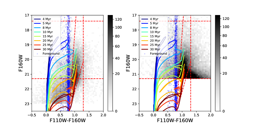
Most notably, we see a high density of HST sources around the red tip of the 10-30 Myr isochrones. The cuts we end up making to isolate that space around the isochrone tips are shown as red dotted lines.
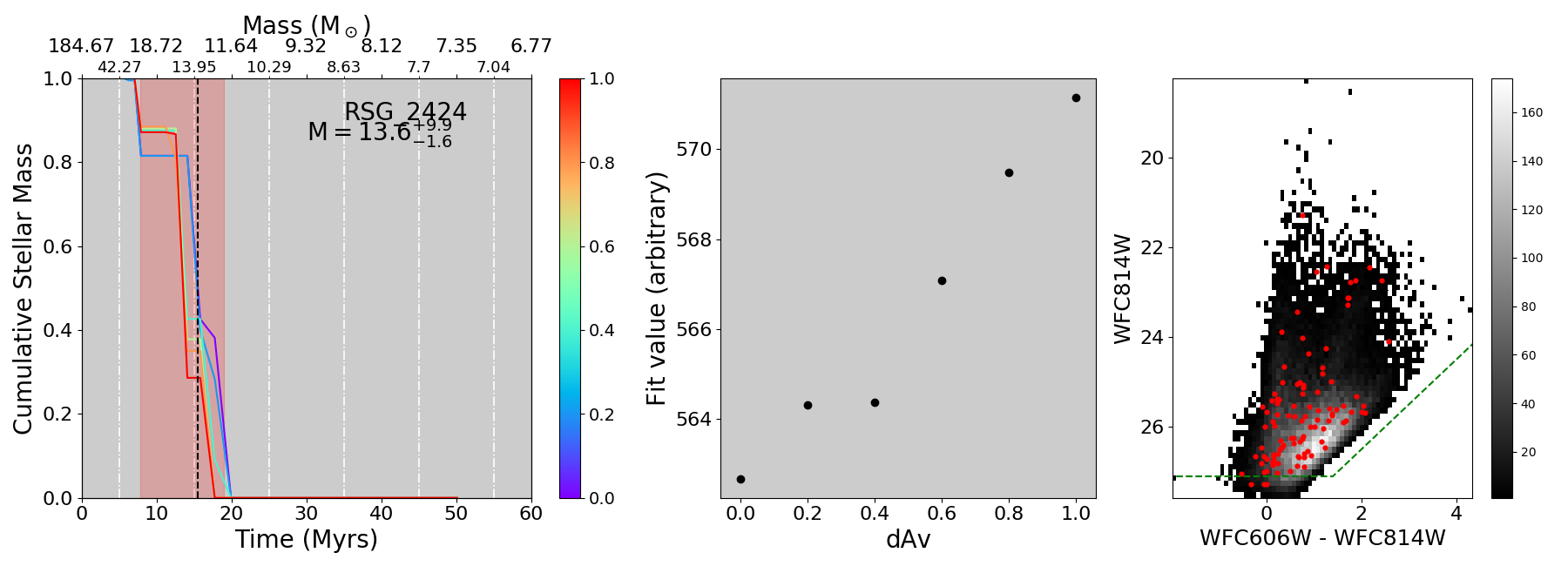
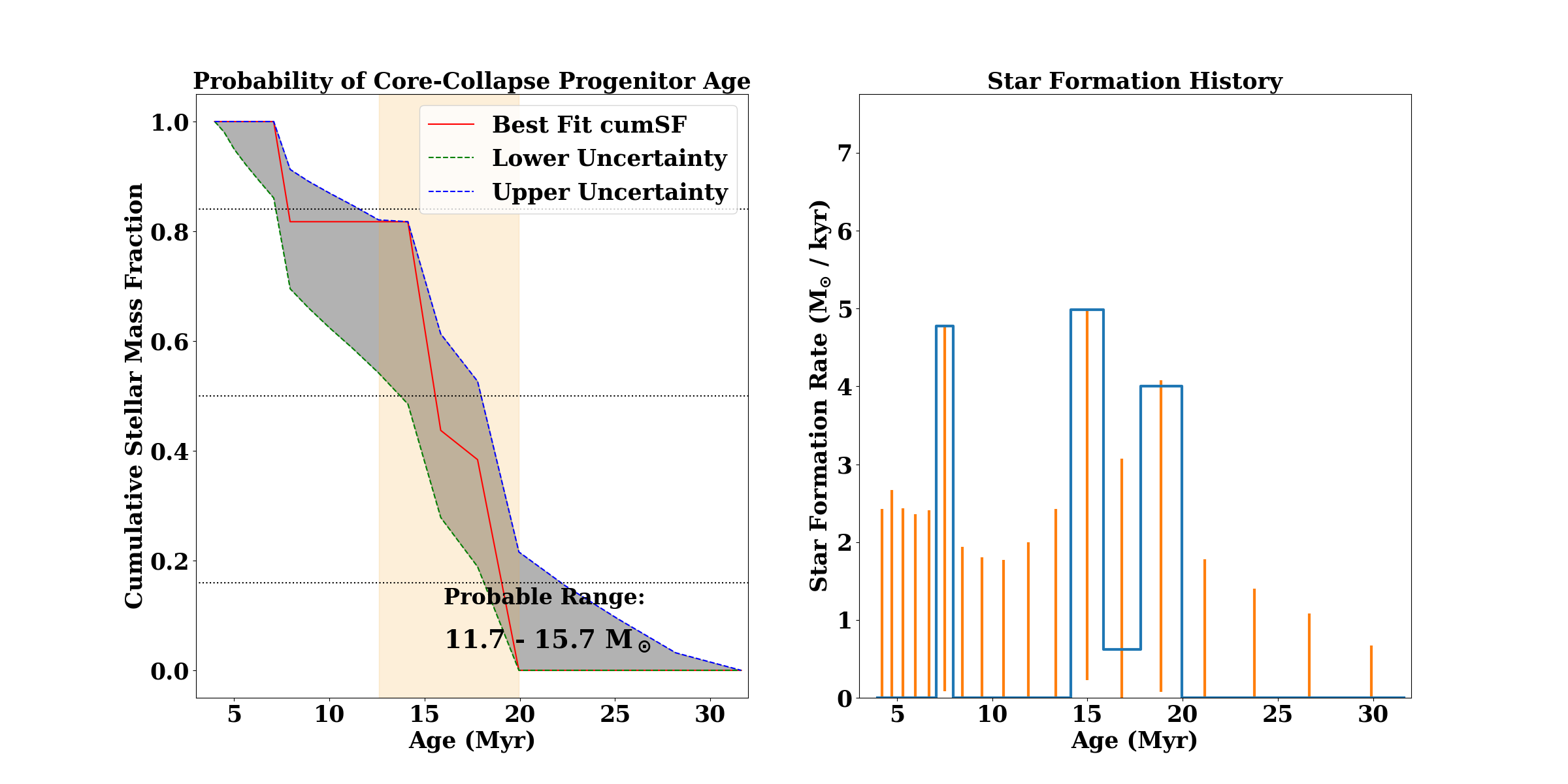
we fed into MATCH to determine SFH. The green dashed line indicates the completeness limits determined by MATCH during the fitting. The gray-scale points are the background sources used to determine the expected population. The bottom set of plots represents a rerun of the output from MATCH in order to determine better constraints on the uncertainties. The method of determining uncertainties is described in Williams et al. (2018). The left plot is similar to the left plot on the top but focuses on the best fit, the uncertainties on that fit only, and the age estimate from the fit. The plot on the right shows the star formation rate at different ages from the population and the uncertainties.

RSG 767 - 9 Myr
RSG 928 - 24 Myr
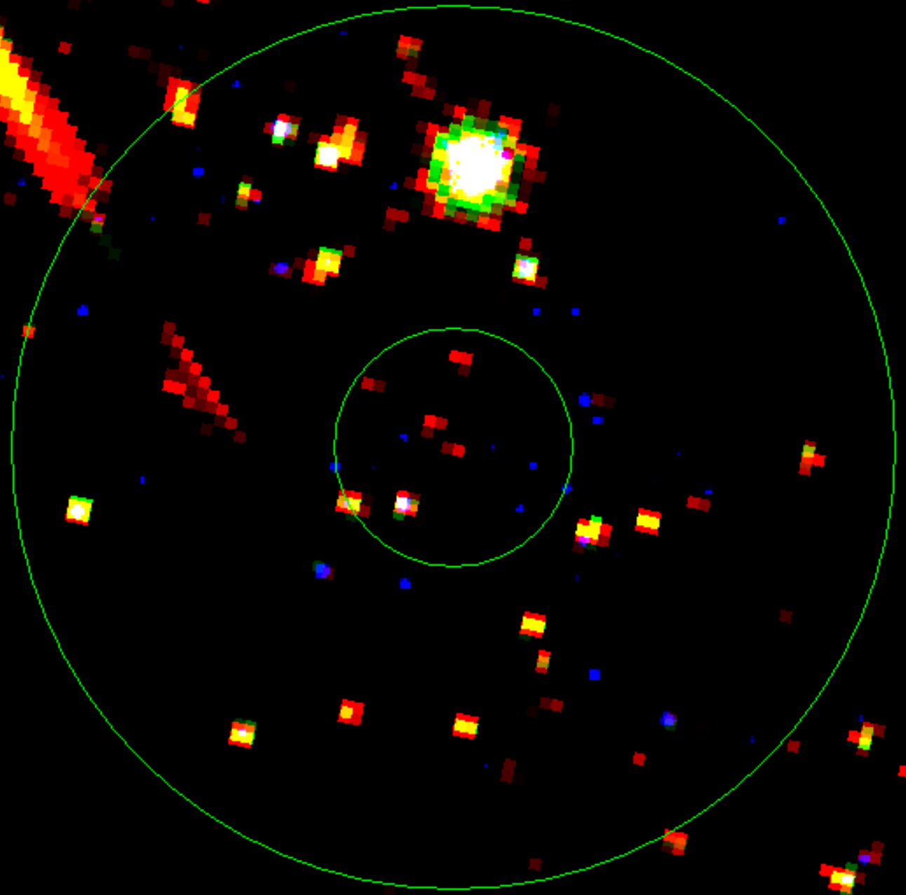
RSG 1282 - 14 Myr
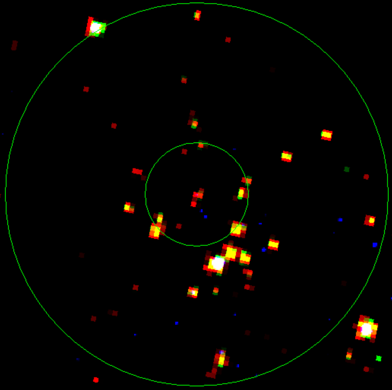
RSG 1321 - 15 Myr
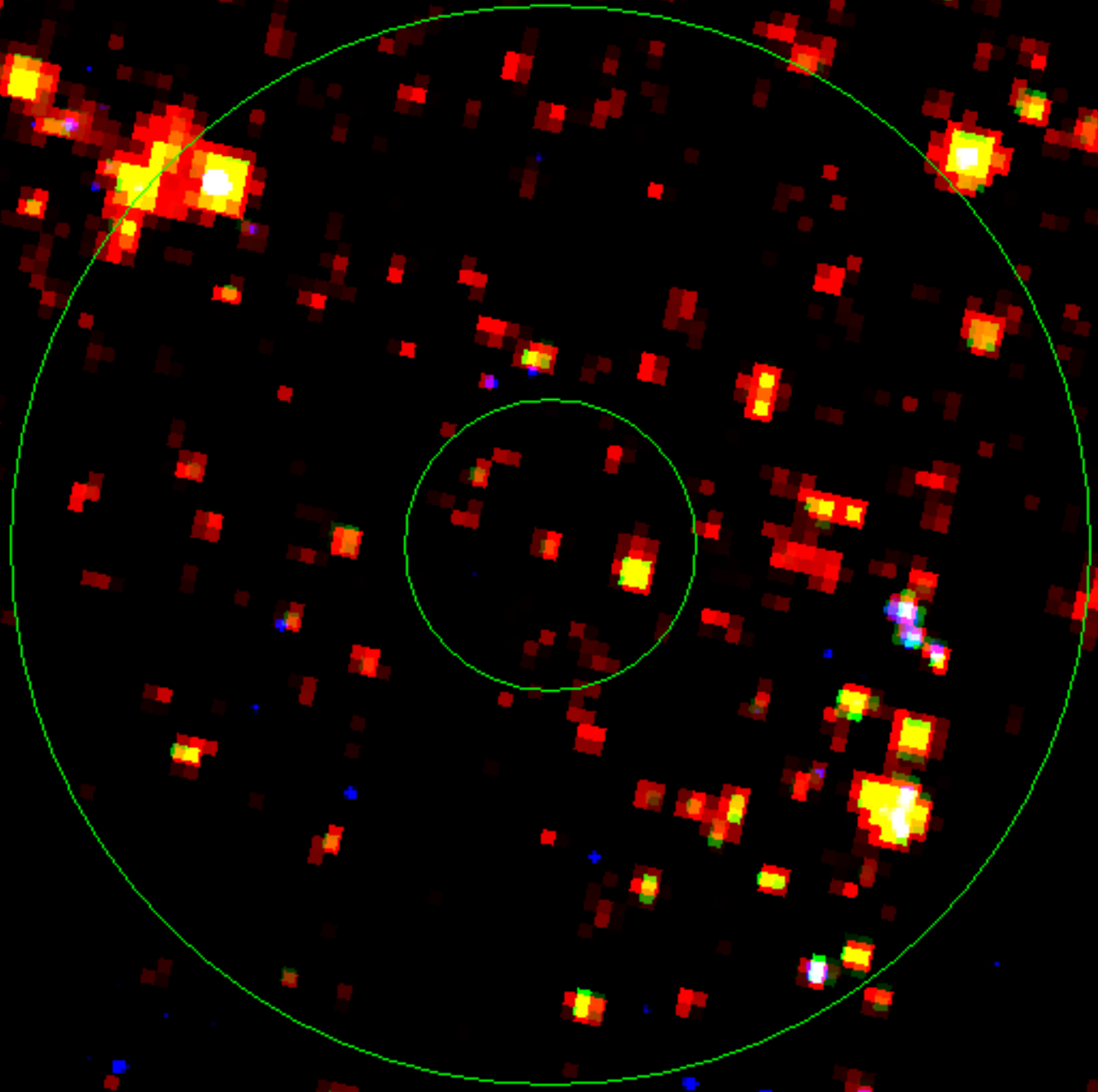
RSG 1355 - 10 Myr
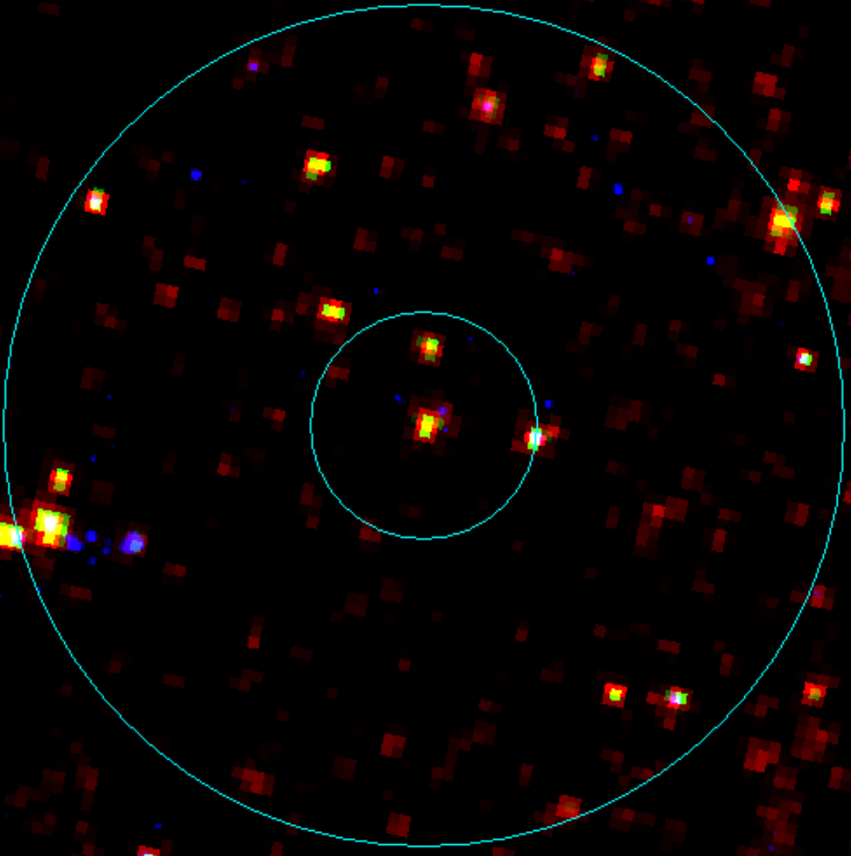
RSG 1534 - 4 Myr
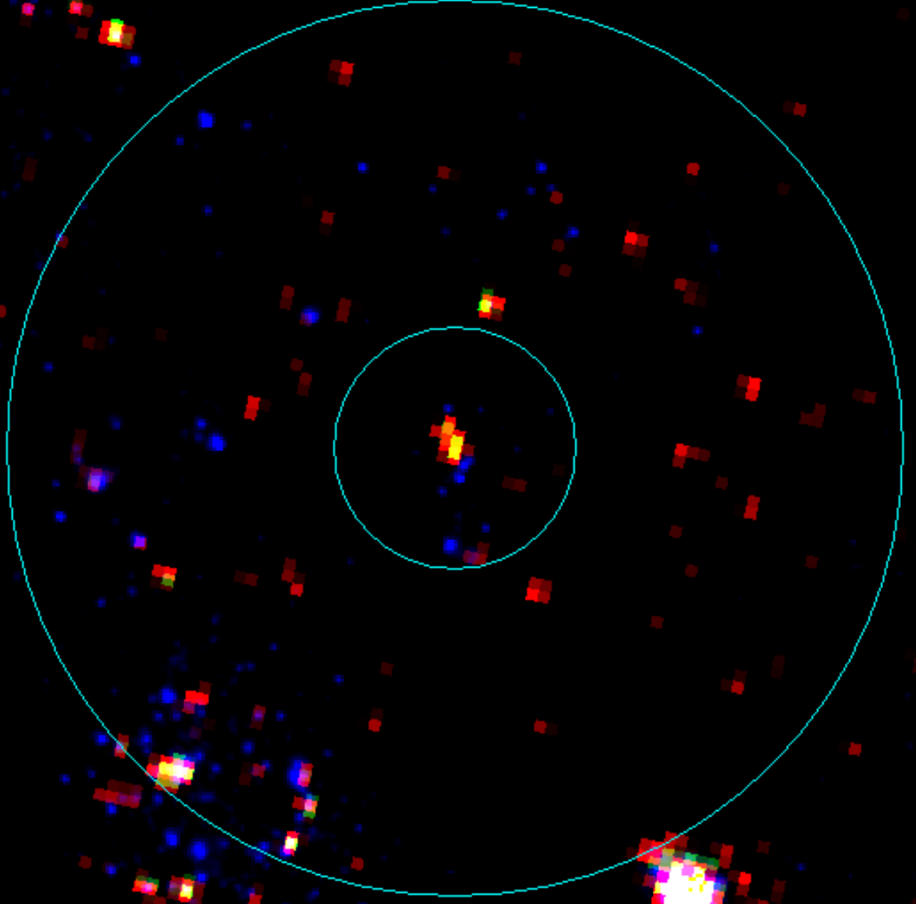
RSG 1539 - 5 Myr
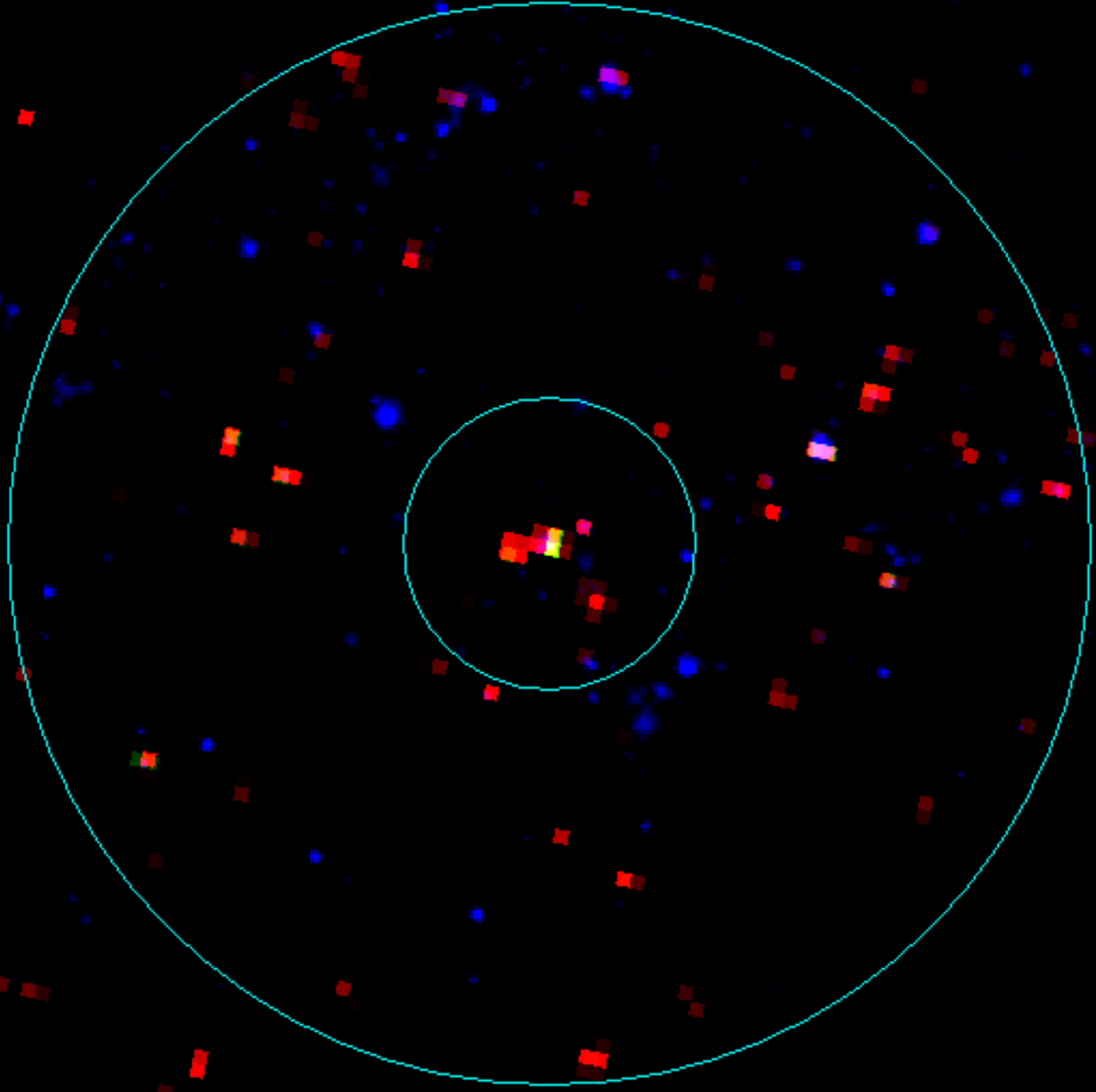
RSG 1661 - 5 Myr
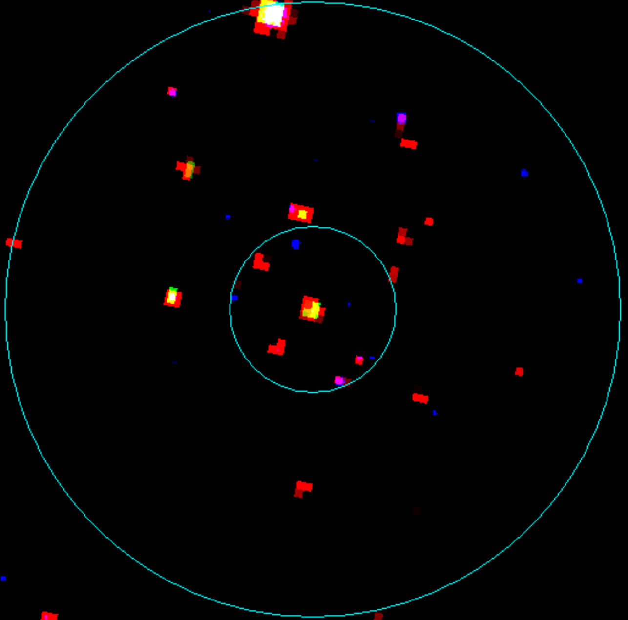
RSG 1966 - 5 Myr
