Enhancing Activity Prediction Models in Drug Discovery with the Ability to Understand Human Language

Abstract

Activity and property prediction models are the central workhorses in drug discovery and materials sciences, but currently they have to be trained or fine-tuned for new tasks. Without training or fine-tuning, scientific language models could be used for such low-data tasks through their announced zero- and few-shot capabilities. However, their predictive quality at activity prediction is lacking. In this work, we envision a novel type of activity prediction model that is able to adapt to new prediction tasks at inference time, via understanding textual information describing the task. To this end, we propose a new architecture with separate modules for chemical and natural language inputs, and a contrastive pre-training objective on data from large biochemical databases. In extensive experiments, we show that our method CLAMP yields improved predictive performance on few-shot learning benchmarks and zero-shot problems in drug discovery. We attribute the advances of our method to the modularized architecture and to our pre-training objective.

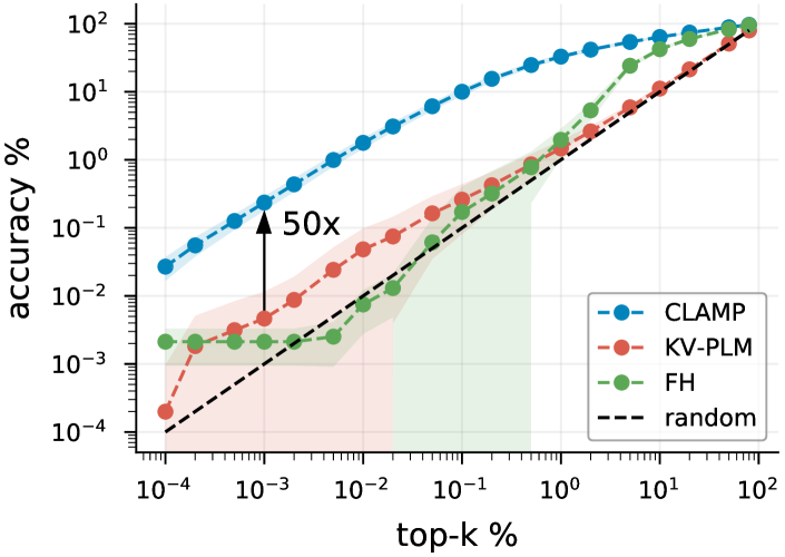
Figure 1: Performance at retrieving active molecules from a chemical database of 1M molecules in a zero-shot setting. Our method CLAMP enriches active molecules for unseen assays by 50x over the next best method KV-PLM (Zeng et al., 2022b), the best-performing scientific language model. Shaded areas represent standard deviation across 2,543 prediction tasks.

Figure 2: Comparison of approaches for activity prediction. a) Activity prediction models use the chemical structure as input and use a molecule encoder to obtain embeddings. b) Scientific language models (SLMs) are able to process biomedical texts that contain both human language and chemical structure. As an example, the displayed text contains a string representation of a molecule CN12..C)NC=N2. SLMs tokenize those strings and treat tokens representing chemical structures in the same way as tokens for natural language. c) Our model, called CLAMP, uses separate encoders for chemical and natural language data and embeds them into a joint embedding space. This allows CLAMP to predict activities for new wet-lab procedures, i.e. bioassays, that are described in human language.

1 Introduction

Activity and property prediction models are the main workhorses in computational drug discovery, and hence are roughly analogous to language models in natural language processing (NLP) and image classification models in computer vision (CV).

The task to predict chemical, macroscopic properties or biological activity of a molecule based on its chemical structure is a decade-old, central problem in natural sciences (Hansch et al., 1962; Hansch, 1969). Machine learning methods have been regularly used to learn these relations between the chemical structure and the properties based on measurement or simulated data since at least the early 90s (King et al., 1993). With the advent of Deep Learning (DL) in drug discovery (Lusci et al., 2013; Dahl et al., 2014; Unterthiner et al., 2014; Chen et al., 2018; Hochreiter et al., 2018) many different molecule encoders (Xu et al., 2019; Mayr et al., 2018; Gilmer et al., 2017) have been suggested that obtain embeddings from chemical structures which are used to predict activities and properties. Activity prediction models are used to select or rank molecules for further biological testing (Melville et al., 2009; Unterthiner et al., 2014) or for flagging or removing molecules with unwanted properties (Mayr et al., 2016). In connection with generative models for molecules (Segler et al., 2018; Gómez-Bombarelli et al., 2018), activity prediction models usually serve as a reward function when the molecule structure should be optimized toward a particular objective (Sanchez-Lengeling & Aspuru-Guzik, 2018; Olivecrona et al., 2017). The combination of activity prediction and generative models has brought a strong speed-up to early phases of drug discovery (Zhavoronkov et al., 2019). As a central tool for drug discovery, activity prediction models are analogous to language models in NLP as well as to image classification models used in computer vision.

Molecule encoders extract relevant features from chemical structures and are trained on bioactivity data.

Activity prediction models based on DL use different low-level or initial descriptions of the chemical structure, such as the molecular graph (Scarselli et al., 2008; Merkwirth & Lengauer, 2005; Kipf & Welling, 2016; Gilmer et al., 2017), the string-representation SMILES (Weininger, 1988; Mayr et al., 2018), chemical fingerprints or descriptors (Dahl et al., 2014; Unterthiner et al., 2014; Mayr et al., 2016), or a combination of those (Yang et al., 2019). While there have been several successes with such DL architectures, such as graph neural networks (GNNs) (Scarselli et al., 2008; Gilmer et al., 2017), their improvements are still disputed and have not been as ground-breaking as for vision and language (Jiang et al., 2021; Bender & Cortés-Ciriano, 2021; Sun, 2022). These activity prediction models are usually trained on pairs of molecules and activity labels from biological experiments, so-called biological assays or bioassays. Bioassays are often wet-lab procedures involving several chemical and biological processing steps, such as growing cell lines and administering chemical agents. Because the labels for the training data points, called bioactivities, are highly time- and cost-intensive to acquire, there has been a considerable interest in being able to efficiently train activity prediction models on few data points. The recently suggested benchmarking dataset FS-Mol (Stanley et al., 2021), provides as few as 16 labeled molecules for an activity prediction task, such that methods must be able to efficiently transfer knowledge from other tasks. Although there would also be substantial information about the activity prediction tasks available in the form of natural language (Kim et al., 2019), the textual description of the biological experiment in the wet-lab, current activity prediction models cannot use this information (Fig. 2a). These models require measurement data from that activity prediction task or bioassay on which they are trained or fine-tuned. Therefore current activity prediction models cannot perform zero-shot activity prediction (Larochelle et al., 2008; Wu et al., 2022) and have limited predictive quality in few-shot settings (Stanley et al., 2021) (Sec. 4).

Scientific language models (SLMs) can utilize both natural language and chemical structure but are suboptimal activity predictors.

Large language models have demonstrated great zero- and few-shot capabilities (Brown et al., 2020; Wei et al., 2021) and they have brought a paradigm-shift for NLP (Sun et al., 2022). Some of these large language models have been also trained on scientific literature (Taylor et al., 2022; Beltagy et al., 2019; Singhal et al., 2022; Edwards et al., 2022), and concretely on biomedical texts (Zeng et al., 2022b), which also contain limited amounts of chemical structures. The SLMs Galactica (Taylor et al., 2022) and KV-PLM (Zeng et al., 2022a) tokenize the SMILES representations of chemical structures and embed those chemical tokens in the same embedding space as language tokens. Therefore, these SLMs can in principle be used to perform zero-shot activity prediction based on the textual description of the bioassay (Fig. 2b). However, SLMs still under-perform at activity prediction (Taylor et al., 2022; Zeng et al., 2022b) (Fig. 1 and Sec. 5), which we attribute to two reasons: a) they are using a sub-optimal molecule encoder, and b) they are trained on overly limited training data. Concerning a), there has been substantial work by the scientific community on finding effective molecule encoders (Gilmer et al., 2017; Wang et al., 2022; Zhu et al., 2022a; Fang et al., 2022; Sun, 2022; Liu et al., 2021; Abdel-Aty & Gould, 2022; Benjamin et al., 2022; He et al., 2022; Rong et al., 2020; Chilingaryan et al., 2022; Winter et al., 2019; Maziarka et al., 2020, 2021; Huang et al., 2021) (Appendix A.9). In comparative studies, the encoder that is implicitly used by the SLMs, i.e., tokenization of SMILES strings with subsequent attention-layers, does not appear as one of the best encoders (Xu et al., 2019; Mayr et al., 2018; Jiang et al., 2021). Concerning b), biomedical texts only contain few tens of thousands of chemical structures, while chemical databases contain hundreds of millions of chemical structures and bioactivities (Kim et al., 2019), which are not used to train SLMs. In summary, we hypothesize that choosing an effective molecule encoder and utilizing chemical databases as training or pre-training data could lead to improved activity prediction.

We propose a modularized architecture with a separate molecule and language encoder and a contrastive learning objective.

In order to i) use an effective molecule encoder, ii) be able to pre-train on data from chemical databases, and iii) to enhance activity prediction models with the ability to utilize human language, we propose an architecture with two separate modules. The first module is a molecule encoder and the second module is a text encoder, that are contrastively pre-trained across these two data modalities (Fig. 2c). Cross-modal contrastive learning (Zhang et al., 2020) and especially Contrastive Language-Image Pre-training (CLIP) (Radford et al., 2021) has strongly impacted several areas of computer vision and NLP. CLIP has brought a tremendous improvement for example for generative models (Ramesh et al., 2022), retrieval systems (Borgeaud et al., 2022), and zero- and few-shot prediction (Radford et al., 2021). One aspect of these successes is that CLIP is modularized: it uses both an effective language encoder (Vaswani et al., 2017; Devlin et al., 2019; Brown et al., 2020) and an effective vision encoder (He et al., 2016). The learning objective of CLIP enables the interaction of these two encoders and a common embedding space of images and language. Furthermore, the success of CLIP rests on the availability of large datasets of pairs of images and text captions (Schuhmann et al., 2022). Both of these aspects, the interaction with predictive or generative models through natural language and the availability of a large dataset of pairs of modalities, could also be beneficial for machine learning systems in drug discovery. At inference time, such a system would be able to acquire new knowledge about a prediction task by accessing the textual description of the bioassay procedure, and thus to predict the activity of molecules without adjusting weights or re-training. This ability could be considered as understanding the bioassay procedure described by human language. The possibility to pre-train this architecture on large chemical databases that contain hundreds of millions of chemical structures paired with textual descriptions of the bioassays, offers an opportunity to train encoders that provide rich representations (Radford et al., 2021).

Our proposed approach unlocks large chemical databases for pre-training.

SLMs are pre-trained on datasets such as ChEBI-20 (Edwards et al., 2021) and ChEBI-22 (Liu et al., 2022a), which comprise only few tens of thousands of molecules. Galactica (Taylor et al., 2022) is additionally trained on the chemical structure of 2M and Grover (Rong et al., 2020) on 10M molecules, however, without associated biological information. In contrast to these pre-training datasets, chemical databases, such as PubChem (Kim et al., 2019) and ChEMBL (Gaulton et al., 2012) contain orders of magnitude more molecules with associated biological information than biomedical texts. The chemical database PubChem contains 114M chemical structures (Kim et al., 2019) and $\sim$300M bioactivity measurements. Additionally, these chemical databases contain textual descriptions of the bioassays that were used to determine the bioactivity of those molecules (Kim et al., 2019). A bioactivity datapoint represents a numeric or binary outcome of bioassay measurement of a molecule, and hence a label for a molecule-text pair. We hypothesize that the chemical databases comprise information that can be leveraged for pre-training cross-modal contrastive learning methods in drug discovery. The amount of information contained in chemical databases could lead to improved molecule encoders and richer representations. To investigate this, we construct a large-scale, open, dataset of chemical structures of molecules and natural language descriptions of bioassays, together with bioactivity measurements from PubChem.

The zero-shot problem in drug discovery is equivalent to the library design problem.

In drug discovery, bioassays take the central role to determine the biological properties of a small molecule, such as inhibitory activity on a drug target in a wet-lab test. A drug target describes a protein whose activity is modulated by a small molecule, whereas a bioassay can measure multiple biological interactions not only constrained to a single protein. New bioassays are often developed with the aim to screen a large library of molecules for a particular activity on a drug target. At this initial phase, when a new bioassay has been developed, the library design problem emerges in all drug discovery projects (Nicolaou & Brown, 2013). The library design problem concerns how to select molecules to be screened without previous experience about the new bioassay (Hajduk et al., 2011; Dandapani et al., 2012; Irwin, 2006), and hence this constitutes a zero-shot prediction problem. A good selection of molecules will lead to a high number of active molecules, which can potentially be further developed into a drug. Therefore, this initial selection of molecules critically determines the success of a drug discovery project and is usually both time- and cost-intensive. The drug discovery process could be made more effective by improving the selection of molecules to be tested in a newly developed bioassay (Sec. 4), which could be tackled with activity prediction models that understand the description of the bioassay procedure. Therefore, we aim at enhancing activity prediction models with the ability to utilize human language.

In summary, our contributions are the following:

• We propose a new architecture for activity prediction that is able to condition on the textual description of the prediction task.

• In contrast to almost all previous approaches, we suggest the use of separate modules for chemical and natural language data.

• We propose a contrastive pre-training objective on information contained in chemical databases as training data. This data contains orders of magnitudes more chemical structures than contained in biomedical texts

• We show that our approach allows for zero-shot activity prediction, yields transferable representations, and improves predictive performance on few-shot benchmarks and zero-shot experiments.

• From a more general perspective, our results show how ML models in application domains can be enhanced with an inferface with human language (Sec. 6).

2 Problem setting: the zero-shot activity prediction in drug discovery

Single-task bioactivity prediction. Bioactivity prediction has been usually considered as a classical supervised, binary prediction prediction task. For a given bioassay or drug target, a machine learning model $\hat{y}=g(m)$ can be trained on a set of available measurement pairs of molecules and activity labels $\{(m_{1},y_{1}),\ldots,(m_{N},y_{N})\}$, where $m_{n}\in\mathcal{M}$ is a representation of a molecule from the chemical space $\mathcal{M}$ and $y_{n}\in\{0,1\}$ is a binary activity label.

Multi-task bioactivity prediction. The problem has also been treated as a multi-task learning problem (Unterthiner et al., 2014; Dahl et al., 2014; Ramsundar et al., 2015; Mayr et al., 2016, 2018), in which several types of activity labels are available for a molecule $\{(m_{1},\bm{y}_{1}),\ldots,(m_{N},\bm{y}_{N})\}$, where $\bm{y}_{n}\in\{0,1\}^{K}$ are vectors containing activity values for $K$ different bioassays or drug targets. The advantage of multi-task learning over single-task is that a learned molecule encoder $\bm{m}=\bm{f}(m)$ can be shared across prediction tasks. However, multi-task deep neural networks (MT-DNN) cannot be used meaningfully for zero-shot transfer learning, when predictions should be made for a new bioassay for which no training data is available.

Zero-shot bioactivity prediction. To allow for zero-shot predictions of new bioassays, for which no training data is available, a textual representation $a$ of the bioassay, which represents the prediction task, can be used. Thus, computational methods are allowed to use both a molecule representation $m$ and a bioassay representation $a\in\mathcal{A}$ from the space $\mathcal{A}$ of textual description of biossays as input. To train such models, the training data can be considered as triplets $\{(m_{1},a_{1},y_{1}),\ldots,(m_{N},a_{N},y_{N})\}$, where $y_{n}\in\{0,1\}\ \forall n$ is a binary activity label, from which the models should learn to provide a prediction $\hat{y}$ based on a new input molecule $m^{*}$ and a new input bioassay $a^{*}$.

3 Contrastive Language-Assay-Molecule Pre-training (CLAMP)

Figure 3: Schematic overview of our approach. CLAMP learns to associate active molecules with their corresponding assay descriptions. The stacked molecule embeddings $\bm{M}=[m_{1},m_{2},m_{3}]$ are contrasted against the bioassay embedding $\bm{a}$. Similar representations in the association space indicate that molecule $m_{1}$ is active, while $m_{3}$ is inactive on bioassay $a$.

Model architecture and objective. Our method uses a trainable molecule encoder $f:\mathcal{M}\mapsto\mathbb{R}^{d}$ to obtain molecule embeddings $\bm{m}=\bm{f}(m)$ and a trainable text encoder $g:\mathcal{A}\mapsto\mathbb{R}^{d}$ to obtain bioassay embeddings $\bm{a}=\bm{g}(a)$. We assume that the embeddings are layer-normalized (Ba et al., 2016). CLAMP also comprises a scoring function $k(\bm{m},\bm{a})$ that should return high values if a molecule $\bm{m}$ is active on a bioassay $\bm{a}$ and low values otherwise. The contrastive learning approach equips our model with the potential for zero-shot transfer learning, that is, supplying meaningful predictions for unseen bioassays.

The CLAMP model has the following structure:

$$\hat{y}=k(\bm{m},\bm{a})=k(\bm{f}(m),\bm{g}(a)),$$ (1)

where $\hat{y}$ is the predicted activity. $k(.,.)$ is a score function that should approximate the targeted distribution $p(y=1\mid\bm{m},\bm{a})$. In practice, we use the following: $k(\bm{m},\bm{a})=\frac{\exp(\tau^{-1}\bm{m}^{T}\bm{a})}{\exp(\tau^{-1}\bm{m}^{T}\bm{a})+1}$, where $\tau^{-1}$ can either be a hyperparameter in the range of $1/\sqrt{d}$ or a learned parameter (Appendix A.4).

The objective of our model is to minimize the following contrastive loss function with respect to $\bm{w}$ and $\bm{v}$ (Gutmann & Hyvärinen, 2010; Mikolov et al., 2013; Lopez-Martin et al., 2021; Jiang et al., 2019; Zang & Wang, 2021; Zhai et al., 2023):

$$\mathrm{L}_{\mathrm{NCE}}=-\frac{1}{N}\sum_{n=1}^{N} y_{n}\log(k(\bm{f}_{\bm{w}}(m_{n}),\bm{g}_{\bm{v}}(a_{n})))+$$

$$(1-y_{n})\log(1-k(\bm{f}_{\bm{w}}(m_{n}),\bm{g}_{\bm{v}}(a_{n})),$$ (2)

where $\bm{f}_{\bm{w}}(.)$ and $\bm{g}_{\bm{v}}(.)$ are neural networks with adjustable weights $\bm{w}$ and $\bm{v}$, respectively. $\{(m_{1},a_{1},y_{1}),\ldots,(m_{N},a_{N},y_{N})\}$ is the training data set of molecule-text-activity triplets (Sec. 2).

The contrastive loss function encourages molecules that are active on a bioassay to have similar embeddings to the embedding of the given bioassay, whereas inactive molecules should have embeddings that are dissimlar to it. In contrast to our approach, in which we have access to many labeled pairs, recent prominent contrastive learning approaches (Radford et al., 2021; Chen et al., 2020) only have access to pairs without label. These methods contrast the matched pair against generated un-matched pairs. Another difference to these methods is that other contrastive learning methods have access to representations of all classes, whereas in our setting of zero-shot transfer learning of bioactivity tasks, only a representation of the positive class, but not of the negative class, is available.

Encoders.Since there are many possible architectures both for the molecule encoder (Xu et al., 2019) as well as for the text encoder, we performed a study in which we assessed different molecule encoders (Appendix A.4 and A.9.4). Molecule encoder. Briefly, for the molecule encoder we tested graph- (Kipf & Welling, 2016), SMILES- (Mayr et al., 2018), and descriptor-based fully-connected architectures (Unterthiner et al., 2014). We found that descriptor-based fully-connected networks as encoders yielded the best performance on a validation set, which is in accordance with recent results on few- and zero-shot drug discovery (Stanley et al., 2021; Jiang et al., 2021; Schimunek et al., 2023). Text encoder. For the text encoder input, we experimented with BioBERT (Lee et al., 2020), Sentence-T5 (Ni et al., 2021) based on T5 (Raffel et al., 2020), KV-PLM (Zeng et al., 2022b), Galactica (Taylor et al., 2022), CLIP text-encoder (Radford et al., 2021), and Latent Semantic Analysis (LSA) (Deerwester et al., 1990) representations of the text. We also consider combinations of these representations. Surprisingly, LSA works well in combinations with language models, which we attribute to the specific characteristics of the language used to describe bioassays (Sec. 6).

Training and hyperparameters. We train the CLAMP architecture from scratch using the AdamW (Loshchilov & Hutter, 2017) optimizer to minimize the objective Eq. (3), and for most cases, a learning rate of 5e-5 is used. The main hyperparameters are the size $d$ of the embedding dimension, the number of layers and neurons of the molecule encoder, the initial assay presentation as well as the initial molecule representation. These hyperparameters are selected on a validation set using manual tuning (Sec. A.4.4).

4 Related work

Scientific language models. Our work is related to scientific language models (SLM) that are able to process chemical inputs. Large language models such as Galactica (Taylor et al., 2022), and KV-PLM (Zeng et al., 2022a) are trained with the usual masking objective (Devlin et al., 2019). MolT5 (Edwards et al., 2022) is using a special objective (Raffel et al., 2020) and also fine-tunes on molecule caption generation. Typically the SLMs’ input tokens represent chemical structures or sub-structures. For example, KV-PLM tokenizes SMILES (Weininger, 1988) strings. The pre-training is done on large sets of scientific (Taylor et al., 2022) or biomedical literature (Zeng et al., 2022a) which contain both natural language and chemical structures.

Activity and property prediction models and few- and zero-shot drug discovery. There is an immense body of works on activity and property prediction models, such that we find it useful refer to survey articles (Muratov et al., 2020; Lo et al., 2018; Walters & Barzilay, 2020; Hochreiter et al., 2018). Since the advent of Deep Learning methods in drug discovery, activity and property prediction models have been strongly improved with respect to predictive quality and thus ranking and selection of molecules with desired activity (Dahl et al., 2014; Unterthiner et al., 2014; Chen et al., 2018; Klambauer et al., 2019; Yang et al., 2019; Walters & Barzilay, 2021). Usually several tens of active and inactive molecules are necessary to train models with a good predictive quality (Mayr et al., 2018; Yang et al., 2019; Sturm et al., 2020). To this end, recent efforts have been undertaken to make Deep Learning models more efficient with respect to the necessary training data (Altae-Tran et al., 2017; Nguyen et al., 2020; Stanley et al., 2021), an area of research which is called few-shot learning or low-resource drug discovery. There are approaches on learning to use protein representations of the drug target together with the chemical structure (van Westen et al., 2011) or to use physical simulations to dock molecules to a protein (Dias et al., 2008), both of which allow for zero-shot activity prediction if the protein target is known. However, these approaches restrict zero-shot activity prediction to the space of bioassays that focus on a particular drug target and exclude all types of functional or toxic activities.

Cross-modal contrastive learning methods and pre-training strategies in drug discovery.

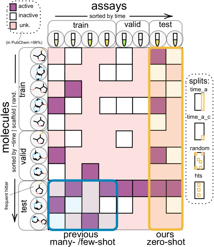
Figure 4: Predictive ability of methods: Rows represent different molecules and columns different bioassays or prediction tasks. While previous methods, e.g. multi-task deep networks, make predictions on unseen molecules and known bioassays (blue box), CLAMP allows to make predictions for molecules on unseen bioassays (yellow box).

Our work is motivated by the advances that cross-modal contrastive learning brought (Radford et al., 2021; Fürst et al., 2022) and is related to cross-modal contrastive learning methods in drug discovery. Usually, one of the data modalities in drug discovery is the chemical structure of the molecule, which is encoded by a molecule encoder. Chang & Ye (2022) contrasts a molecular property vector with a SMILES encoder. Guo et al. (2022) contrasts the IUPAC International Chemical Identifier (InChi) with a SMILES encoder. Zhu et al. (2022a) contrasts different representations including SMILES, FP, 3D-geometry, of molecules with each other. The second modality could be natural language (Zeng et al., 2022a; Edwards et al., 2021) but also other modalities such as chemical reaction-templates (Seidl et al., 2022), microscopy images (Sanchez-Fernandez et al., 2022), proteins (Li et al., 2022) or different molecular representations have been suggested. Edwards et al. (2021) contrasts molecules with textual descriptions and constructs a dataset of 33k corresponding molecule and text descriptions termed ChEBI-20. Liu et al. (2022b) contrast molecules with a corresponding text from proposed dataset PubChemSTM with 280K text-molecule pairs. Further related work in Sec. A.1.

5 Experiments and Results

To demonstrate the effectiveness of our method, we performed three sets of experiments: a) Zero-shot transfer learning: In this experiment, we test the ability of methods to predict the activity of molecules on a bioassay of which only a textual description is available. This setting assesses whether models are able to acquire new knowledge on the prediction task from the textual bioassay description. The usual activity prediction models (Fig. 2) cannot perform this task, but SLMs have shown some capabilities. b) Representation learning: To check whether the learned molecule representations of different methods are rich and transferable, we perform linear probing on a variety of benchmarking datasets (Wu et al., 2018). c) Retrieval and library design: In this third experiment, we demonstrate the use of our method as a retrieval system. Based on the bioassay representation, molecules can be retrieved from a chemical database and then ranked for wet-lab testing. We supply several additional experiments in Sec. A.9.

Table 1: Zero-shot results of different methods on four different datasets. Green cells indicate the highest values and values within yellow cells are within the standard-deviation to the highest value. Error bars represent standard deviations across the five training re-runs (if computationally feasible). Results are reported in %.

metric	dataset	split	random	GAL 125M†	KV-PLM†	1-NN	soft-NN	FH	CLAMP
$\Delta$AP	FS-Mol	default	${01.57^{\pm{0.3}}}$	${01.44^{\pm{0.0}}}$	${01.84^{\pm{0.0}}}$	${14.68^{\pm{0.7}}}$	${13.81^{\pm{1.8}}}$	${18.50^{\pm{0.2}}}$	${19.37^{\pm{0.2}}}$
	PubChem	hts	${00.01^{\pm{0.0}}}$	${00.00^{\pm{0.0}}}$	${00.10^{\pm{0.0}}}$	${01.20^{\pm{0.1}}}$	${02.04^{\pm{0.4}}}$	${03.10^{\pm{0.1}}}$	${08.43^{\pm{0.1}}}$
		time_a	${02.13^{\pm{0.3}}}$	${01.39^{\pm{0.0}}}$	${03.57^{\pm{0.0}}}$	${12.96^{\pm{1.0}}}$	${05.67^{\pm{0.7}}}$	${10.23^{\pm{0.5}}}$	${14.77^{\pm{0.3}}}$
		time_a_c	${04.39^{\pm{0.5}}}$	${04.20^{\pm{0.0}}}$	${07.99^{\pm{0.0}}}$	${11.11^{\pm{0.3}}}$	${06.99^{\pm{2.8}}}$	${10.35^{\pm{0.9}}}$	${11.67^{\pm{0.6}}}$
AUROC	FS-Mol	default	${50.24^{\pm{0.4}}}$	${50.50^{\pm{0.0}}}$	${50.56^{\pm{0.0}}}$	${64.69^{\pm{0.8}}}$	${63.92^{\pm{1.9}}}$	${68.22^{\pm{0.2}}}$	${69.26^{\pm{0.2}}}$
	PubChem	hts	${49.92^{\pm{0.2}}}$	${49.32^{\pm{0.0}}}$	${49.65^{\pm{0.0}}}$	${67.92^{\pm{0.8}}}$	${68.41^{\pm{0.9}}}$	${73.48^{\pm{0.4}}}$	${73.83^{\pm{0.3}}}$
		time_a	${50.08^{\pm{0.5}}}$	${47.05^{\pm{0.0}}}$	${54.92^{\pm{0.0}}}$	${66.53^{\pm{0.6}}}$	${57.85^{\pm{1.7}}}$	${66.77^{\pm{1.5}}}$	${68.66^{\pm{0.5}}}$
		time_a_c	${49.91^{\pm{0.4}}}$	${48.04^{\pm{0.0}}}$	${57.00^{\pm{0.0}}}$	${61.98^{\pm{0.4}}}$	${55.06^{\pm{6.3}}}$	${61.65^{\pm{0.8}}}$	${63.66^{\pm{0.4}}}$

^† for the SLMs, we chose a single model provided by the authors. Training re-runs are computationally infeasible (see Sec. A.10).

Metrics. We compare different methods for their ability to rank active molecules higher than inactive molecules. Due to the imbalanced nature of the prediction tasks, usually the frequency of inactive molecules is much higher than that of active molecules. We use delta average precision ($\Delta$AP) as main metric (Stanley et al., 2021) in Experiments a) and b) and the enrichment factor (EF) (Friesner et al., 2004) as metric for experiment c) (see Sec. A.3),

5.1 Zero-Shot Transfer

All methods have to predict the activity of molecules for new activity prediction tasks based on the textual description of the task without any available labels for that task. This setting represents a zero-shot problem in drug discovery.

Datasets. To this end, we use the benchmarking dataset FS-Mol (Stanley et al., 2021) and propose a zero-shot mode. Further, we construct three different splits of the PubChem (Kim et al., 2019) database (Fig. 4): the "hts" split contains high-throughput assays (Laufkötter et al., 2019), the "time_a" split contains assays sorted by time. We test on 4,201 assays from 2013-11 to 2018-05. For the "time_a_c" split, we additionally sort compounds by time and test on new unseen molecules from new assays.

Methods compared. We compared the method CLAMP, the following baseline methods and competitor methods: 1-nearest-neighbour (1-NN): this method uses textual description of the given bioassay, to identify the most similar bioassay in the training set. Then the predictions for this training set assay are used for the given prediction task. The predictions are based on a MT-DNN. soft-nearest-neighbour (soft-NN): Uses the same approach as 1-NN only that the predictions of the training set assay are weighted by their similarity to the given assay. The last baseline is the so-called Frequent hitters (FH) model (Schimunek et al., 2023): this model predicts the general activity of a molecule across all prediction task. This is a strong baseline, since there are molecule that often test positive in any bioassay (Baell & Holloway, 2010). Another category of methods that are able to perform zero-shot activity predictions are SLMs that are able to process chemical structures: The SLM Galactica (GAL 125M) has been included with an appropriate text prompt (Appendix A.6.1) and also the SLM KV-PLM. We use the publicly available SLMs that were pre-trained on their suggested text corpora. For details, see Appendix A.6.

Results. The results are shown in Tab. 1. CLAMP significantly outperforms all other methods with respect to $\Delta$AP (paired Wilcoxon test) except the FH models on the "hts" and "time_a_c" splits. Notably, the SLMs do not reach the predictive performance of the FH baseline that completely ignores the textual information.

5.2 Representation Learning

Table 2: Linear probing results of different methods with respect to $\Delta$AP. Green cells indicate the highest values in a category of tasks and areas in yellow cells within the standard-deviation to the maximum value. Because of the low variability of training re-runs of a linear probing model, the error bars represents standard-deviation obtained through bootstrap resampling. Rank-avg represents the mean rank over all assays. Methods are assigned to categories (cat): self-supervised learning methods (SSL), scientific lanuage models (SLM), and chemical descriptors or fingerprints (FP)

dataset		BACE	BBBP	ClinTox	HIV	SIDER	Tox21	ToxCast	Tox21-10k
split		scaffold	scaffold	scaffold	scaffold	scaffold	scaffold	scaffold	original
# of assays	cat	1	1	2	1	27	12	617	68	rank-avg
CLAMP	ours	${27.47^{\pm{\scriptscriptstyle 4}}}$	${16.47^{\pm{\scriptscriptstyle 4}}}$	${11.05^{\pm{\scriptscriptstyle 6}}}$	${28.49^{\pm{\scriptscriptstyle 4}}}$	${08.96^{\pm{\scriptscriptstyle 4}}}$	${23.35^{\pm{\scriptscriptstyle 6}}}$	${09.44^{\pm{\scriptscriptstyle 5}}}$	${51.27^{\pm{\scriptscriptstyle 10}}}$	${02.85^{\pm{\scriptscriptstyle 2}}}$
Grover	SSL	${21.74^{\pm{\scriptscriptstyle 4}}}$	${16.76^{\pm{\scriptscriptstyle 4}}}$	${22.74^{\pm{\scriptscriptstyle 8}}}$	${13.58^{\pm{\scriptscriptstyle 3}}}$	${05.41^{\pm{\scriptscriptstyle 4}}}$	${12.88^{\pm{\scriptscriptstyle 5}}}$	${05.22^{\pm{\scriptscriptstyle 3}}}$	${42.23^{\pm{\scriptscriptstyle 10}}}$	${05.08^{\pm{\scriptscriptstyle 3}}}$
Mc+RDKc	FP	${23.87^{\pm{\scriptscriptstyle 4}}}$	${18.39^{\pm{\scriptscriptstyle 4}}}$	${17.75^{\pm{\scriptscriptstyle 7}}}$	${25.57^{\pm{\scriptscriptstyle 4}}}$	${08.43^{\pm{\scriptscriptstyle 4}}}$	${13.96^{\pm{\scriptscriptstyle 5}}}$	${05.18^{\pm{\scriptscriptstyle 4}}}$	${42.45^{\pm{\scriptscriptstyle 10}}}$	${05.64^{\pm{\scriptscriptstyle 3}}}$
CDDD	SSL	${17.51^{\pm{\scriptscriptstyle 5}}}$	${20.56^{\pm{\scriptscriptstyle 4}}}$	${33.82^{\pm{\scriptscriptstyle 7}}}$	${12.29^{\pm{\scriptscriptstyle 3}}}$	${05.30^{\pm{\scriptscriptstyle 4}}}$	${10.34^{\pm{\scriptscriptstyle 4}}}$	${04.82^{\pm{\scriptscriptstyle 3}}}$	${36.32^{\pm{\scriptscriptstyle 9}}}$	${05.79^{\pm{\scriptscriptstyle 3}}}$
BARTSmiles	SSL	${29.16^{\pm{\scriptscriptstyle 3}}}$	${17.09^{\pm{\scriptscriptstyle 4}}}$	${10.94^{\pm{\scriptscriptstyle 6}}}$	${07.88^{\pm{\scriptscriptstyle 2}}}$	${05.24^{\pm{\scriptscriptstyle 4}}}$	${10.34^{\pm{\scriptscriptstyle 4}}}$	${05.07^{\pm{\scriptscriptstyle 3}}}$	${30.40^{\pm{\scriptscriptstyle 9}}}$	${05.79^{\pm{\scriptscriptstyle 3}}}$
KV-PLM	SLM	${24.44^{\pm{\scriptscriptstyle 4}}}$	${17.61^{\pm{\scriptscriptstyle 4}}}$	${07.08^{\pm{\scriptscriptstyle 4}}}$	${06.20^{\pm{\scriptscriptstyle 2}}}$	${04.61^{\pm{\scriptscriptstyle 4}}}$	${09.90^{\pm{\scriptscriptstyle 4}}}$	${04.53^{\pm{\scriptscriptstyle 3}}}$	${30.92^{\pm{\scriptscriptstyle 10}}}$	${05.88^{\pm{\scriptscriptstyle 3}}}$
MFBERT	SSL	${14.89^{\pm{\scriptscriptstyle 4}}}$	${19.77^{\pm{\scriptscriptstyle 4}}}$	${11.84^{\pm{\scriptscriptstyle 7}}}$	${06.09^{\pm{\scriptscriptstyle 1}}}$	${06.93^{\pm{\scriptscriptstyle 4}}}$	${08.46^{\pm{\scriptscriptstyle 4}}}$	${04.72^{\pm{\scriptscriptstyle 3}}}$	${25.61^{\pm{\scriptscriptstyle 8}}}$	${06.20^{\pm{\scriptscriptstyle 3}}}$
Graphormer	SSL	${20.22^{\pm{\scriptscriptstyle 4}}}$	${08.67^{\pm{\scriptscriptstyle 4}}}$	${04.51^{\pm{\scriptscriptstyle 4}}}$	${06.87^{\pm{\scriptscriptstyle 2}}}$	${05.71^{\pm{\scriptscriptstyle 4}}}$	${08.16^{\pm{\scriptscriptstyle 4}}}$	${04.10^{\pm{\scriptscriptstyle 3}}}$	${29.50^{\pm{\scriptscriptstyle 9}}}$	${06.55^{\pm{\scriptscriptstyle 3}}}$
Morgan	FP	${27.79^{\pm{\scriptscriptstyle 4}}}$	${16.06^{\pm{\scriptscriptstyle 4}}}$	${23.86^{\pm{\scriptscriptstyle 8}}}$	${16.23^{\pm{\scriptscriptstyle 4}}}$	${06.97^{\pm{\scriptscriptstyle 4}}}$	${09.69^{\pm{\scriptscriptstyle 4}}}$	${04.28^{\pm{\scriptscriptstyle 3}}}$	${36.07^{\pm{\scriptscriptstyle 10}}}$	${06.64^{\pm{\scriptscriptstyle 3}}}$
MolT5	SLM	${11.51^{\pm{\scriptscriptstyle 4}}}$	${16.03^{\pm{\scriptscriptstyle 4}}}$	${10.06^{\pm{\scriptscriptstyle 6}}}$	${15.92^{\pm{\scriptscriptstyle 3}}}$	${02.91^{\pm{\scriptscriptstyle 3}}}$	${06.20^{\pm{\scriptscriptstyle 3}}}$	${03.53^{\pm{\scriptscriptstyle 3}}}$	${15.65^{\pm{\scriptscriptstyle 6}}}$	${07.36^{\pm{\scriptscriptstyle 3}}}$
MolCLR	SSL	${15.59^{\pm{\scriptscriptstyle 4}}}$	${13.01^{\pm{\scriptscriptstyle 4}}}$	${00.99^{\pm{\scriptscriptstyle 3}}}$	${02.57^{\pm{\scriptscriptstyle 1}}}$	${06.13^{\pm{\scriptscriptstyle 4}}}$	${06.08^{\pm{\scriptscriptstyle 3}}}$	${02.43^{\pm{\scriptscriptstyle 2}}}$	${13.21^{\pm{\scriptscriptstyle 5}}}$	${08.20^{\pm{\scriptscriptstyle 3}}}$

In this experiment, we use linear probing (Alain & Bengio, 2016) to assess how robust and transferable the embeddings of different encoders are.

Datasets. We use the MoleculeNet (Wu et al., 2018) benchmarking datasets, BACE, BBBP, ClinTox, HIV, SIDER, Tox21 and ToxCast. Additionally, we compare methods on Tox21-10k (Richard et al., 2021). We remove all downstream test-set molecules from the pre-training dataset (Sec. A.2.4).

Methods compared. Molecular encoders are pre-trained in their proposed way. CLAMP was pre-trained on PubChem with a random split and we removed all test-set-molecules that are contained in the downstream tasks to avoid data leakage (Appendix A.2.4). We included several baseline encoders, that extract substructures from molecules, that is, Morgan fingerprints (Morgan, 1965) of length 1024, and a combination of those with chemical descriptors (Landrum, 2013) Mc+RDKc of length 8192. Furthermore, the following molecule encoders that were pre-trained in self-supervised fashion were assessed: Grover (Rong et al., 2020), a graph transformer, CDDD (Winter et al., 2019), a SMILES-LSTM based autoencoder, the SMILES-Tranformers BARTSmiles (Chilingaryan et al., 2022), Graphormer (Ying et al., 2021), MFBERT (Abdel-Aty & Gould, 2022), and MolCLR (Wang et al., 2021b), a contrastively pre-trained GNN. We also use the SLMs KV-PLM (Zeng et al., 2022b), MolT5 (Edwards et al., 2022) and Galactica (Taylor et al., 2022).

Results. Tab. 2 displays the results of different methods on the linear probing experiments with respect to $\Delta$AP. CLAMP performs best on average and significantly (paired Wilcoxon test; all $p$-values $<$1e-10) outperforms all other methods with respect to $\Delta AP$ across prediction tasks. Our method yields the best performing representations in 5 of the 8 datasets, and the datasets on which CLAMP is not the best method, it is within the standard-deviation. Notably, CLAMP strongly improves predictive performance on on ToxCast from a $\Delta AP$ of $05.22^{\pm 3}$ to $09.44^{\pm 5}$, which is an average over 617 prediction tasks.

5.3 Retrieval and library design

Here we consider a retrieval task, in which molecules from a chemical database must be ranked based on a given bioassay that represents the query. Molecules that are active on the given bioassay should be ranked high. The enrichment-factor (EF) is used as metric to evaluate this type of retrieval tasks (Truchon & Bayly, 2007). The EF calculates how much a given method improves the top-$k$ accuracy over a random ordering for a given $k$.

Dataset. We use the PubChem dataset with assay based temporal split time_a. For molecule retrieval, we chose the assay-based temporal split time_a (Appendix A.2). For the chemical databases we consider two sizes: 1M or 10k molecules. Molecules have been selected in order of their PubChem compound-ID (CID). To obtain robust estimates, we consider assays with more than 100 active molecules and report the average over assays. This results in 190 assays for the 10k molecules setting and 2,543 assays for the 1M molecule setting for testing.

Methods compared. The methods CLAMP and FH are trained on the time_a split and chosen based on validation $\Delta AP$. For FH baseline the ranking for the molecules remains the same regardless of the assay. We benchmarked against KV-PLM and Galactica. Evaluating Galactica on the 1M benchmark is computationally infeasible (Appendix A.10) because for each combination a full forward-pass has to be performed. At the 10k setting, it takes $\sim$13sec for KV-PLM, $\sim$9sec for CLAMP and $\sim$19h for GAL for 190 assays.

Results. We find that CLAMP enriches active molecules for unseen assays by more than 10-fold in the case of 10k, and by more than 250-fold in the case of 1M molecules. KV-PLM (Zeng et al., 2022b), the best- performing scientific language model is outperformed by 50x (Fig. 1). Fig. A7 shows a comparison between the methods across different top-$k$ accurracies. CLAMP consistently outperforms all other methods.

6 Discussion

Conclusions. Our proposed contrastive learning method CLAMP exhibits the best performance at zero-shot prediction drug discovery tasks on several large datasets. The pre-trained molecule-encoder of CLAMP yields transferable representations. Our results also point out that, although the scientific language models can in principle be used for zero-shot activity prediction, they are not performing well at this task and are computationally demanding (Sec. 5.3). Limitations and Future work. Currently, our approach is mostly limited by computational complexity, since both hyperparameter and model selection is computationally demanding. We leave it to future work, to expand on the search for different encoders in conjunction with our approach. The models can perform activity prediction, but is not able to generate molecules. However, the embedding space of CLAMP is a prime candidate for conditional generation as it is analogous to the CLIP latent space (Ramesh et al., 2022). Chemical dosage, which affects the assay outcome, as with many other approaches, is not considered. It may also struggle with negations and grammatical nuances, resulting in inaccurate predictions. As for all ML methods, the predictive ability of CLAMP can decrease outside the chemical and bioassay space of the training data and suffers from biases that are present in chemical databases. Broader impact. See Sec. A.11.

Data and software availability. Python code and instructions to reproduce the results are provided as Supplementary Material and will be available at https://github.com/ml-jku/clamp

Acknowledgments The ELLIS Unit Linz, the LIT AI Lab, the Institute for Machine Learning, are supported by the Federal State Upper Austria. IARAI is supported by Here Technologies. We thank the projects AI-MOTION (LIT-2018-6-YOU-212), DeepFlood (LIT-2019-8-YOU-213), Medical Cognitive Computing Center (MC3), INCONTROL-RL (FFG-881064), PRIMAL (FFG-873979), S3AI (FFG-872172), DL for GranularFlow (FFG-871302), EPILEPSIA (FFG-892171), AIRI FG 9-N (FWF-36284, FWF-36235), ELISE (H2020-ICT-2019-3 ID: 951847), Stars4Waters (HORIZON-CL6-2021-CLIMATE-01-01). We thank Audi.JKU Deep Learning Center, TGW LOGISTICS GROUP GMBH, Silicon Austria Labs (SAL), FILL Gesellschaft mbH, Anyline GmbH, Google, ZF Friedrichshafen AG, Robert Bosch GmbH, UCB Biopharma SRL, Merck Healthcare KGaA, Verbund AG, GLS (Univ. Waterloo) Software Competence Center Hagenberg GmbH, TÜV Austria, Frauscher Sensonic and the NVIDIA Corporation.

Appendix A Appendix

A.1 Further related work

Zero-shot learning problems.

From the perspective of machine-learning, the described problem represents a zero-data or zero-shot prediction task (Chang et al., 2008; Larochelle et al., 2008; Farhadi et al., 2009; Palatucci et al., 2009), for which several methods in the area of computer vision and natural language processing have been developed (Wang et al., 2019). The setting is that no training data are available and only a description of the classes or tasks are provided, which in our case is the textual description of the bioassay. In contrast to zero-shot problems in computer vision where a description of each class is available, in the drug discovery setting only a description of the positive class is available. Contrastive learning for zero-data problems has recently been exemplified with the ConVIRT (Zhang et al., 2020) or the CLIP algorithm (Radford et al., 2021), in which representations of natural images and language are learned.

Proteo-chemometric and molecular docking.

Several efforts have been devoted to being able to make predictions for new biological targets, such as proteins. The set of proteochemometric methods (van Westen et al., 2011) use information about the protein, such as its 1D structure, and combine it with information about the molecule. Molecular docking methods use the 3D structure of the protein and search for a conformation of a ligand that fits into a binding pocket (Pagadala et al., 2017; Meng et al., 2011). However, many bioassays are not focused on a target, but rather measure a general effect, such as a toxic response or cell proliferation, which limits or prohibits the use of proteochemic or docking methods.

Recommender systems.

The zero-data problem has earlier been identified by the recommender systems and matrix factorization research community as cold-start problem (Schein et al., 2002). The cold-start problem is how to to provide good recommendations for novel users or items. Remedies for the cold-start problem of recommender systems exploit similarities of initial descriptions between users and items (Lika et al., 2014). Contrastive learning has recently been suggested to learn the similarities between users and items (Liu et al., 2021; Zhou et al., 2020). From the perspective of recommender systems, our method CLAMP can be understood as having to suggest molecules representing items for a new bioassay representing a new user.

Selection strategies for bioassay screening.

Our approach is related to works on different strategies for selecting a molecule library for wet-lab testing. A prominent approach is high-throughput screening, in which large parts of physically available molecules are screened at high-throughput (Hajduk et al., 2011). This is possible if the bioassay can be performed in high throughput, the wet-lab facilities and a large molecule library are available. High-throughput screening has been seen as a strong improvement in drug discovery. Naturally, many computational methods have also been suggested to first virtually screen (Shoichet, 2004) chemical libraries and then perform bioassay screening on the top-ranked molecules. Data-driven strategies, such as machine learning and Deep Learning, have brought a strong improvement of virtual screening methods. However, data-driven strategies are not possible for new bioassays (Ain et al., 2015) since no data is available, and no actives or inactives are known. To ameliorate this central problem, practitioners and scientists have resorted to using information from similar bioassays, facilitated by efforts to semantically structure the information about bioassays (Visser et al., 2011). However, this type of information has not been integrated into machine learning approaches yet. In summary, while data-driven virtual screening strategies have been shown to be highly effective, it is currently unclear how those approaches could be used for designing libraries for newly developed bioassays.

Information from the textual description of the bioassay can be leveraged with contrastive learning.

Despite the lack of known active and inactive molecules for novel bioassays, there is information available that could potentially be used for machine learning: the textual description of the bioassay. For each bioassay, the procedure in the wet-lab, their endpoint, and the substrate, are usually described in textual form. There have even been efforts to semantically describe such bioassays using an ontology (Visser et al., 2011).

A.2 Datasets

Here we provide an overview of the datasets used in this work. The summary statistics can be found in Tab. A3.

Table A3: Main datasets summary statistics overview.

	PubChem	PubChem HTS	FS-Mol
Source	PubChem	PubChem	ChEMBL27
# measurements	223,219,241	143,886,653	501,366
# molecules	2,120,811	715,231	240,465
# assays	21,002	582	5,135
% of assays with only one class	74.54	1.37	0.00
Mean # compounds / assay	10,628.48	247,227.93	96.32
Median # compounds / assay	35.00	304,804.00	46.00
% active	1.51	0.70	46.48
% density	0.50	34.57	0.04
Mean % active per assay	79.46	1.04	47.17
Median % active per assay	100.00	0.42	48.84

A.2.1 An open, large-scale dataset for zero-shot drug discovery derived from PubChem

We constructed a large public dataset extracted from PubChem (Kim et al., 2019; Preuer et al., 2018), an open chemistry database, and the largest collection of readily available chemical data. We take assays ranging from 2004 to 2018-05. It initially comprises 224,290,250 records of molecule-bioassay activity, corresponding to 2,120,854 unique molecules and 21,003 unique bioassays. We find that some molecule-bioassay pairs have multiple activity records, which may not all agree. We reduce every molecule-bioassay pair to exactly one activity measurement by applying majority voting. Molecule-bioassay pairs with ties are discarded. This step yields our final bioactivity dataset, which features 223,219,241 records of molecule-bioassay activity, corresponding to 2,120,811 unique molecules and 21,002 unique bioassays ranging from AID 1 to AID 1259411. Molecules range up to CID 132472079. The dataset has 3 different splitting schemes which are further described in Sec. A.2.5.

A.2.2 FS-Mol

The FS-Mol dataset (Stanley et al., 2021) has been constructed based on ChEMBL (Gaulton et al., 2012) with the focus on providing a few-shot learning dataset to the research community. The dataset comprises $\sim$240k molecules and 5k prediction tasks, roughly equivalent to bioassays. In the original form of FS-Mol, for each prediction task a small training set (support-set) of 16, 32, 64, or 128 molecules together with binary activity labels are available for few-shot learning.

We extend the dataset with textual descriptions sourced from ChEMBL. We further use this dataset in a zero-shot setting, where we only have the text description of the prediction task available (examples in Tab. A5). For the standard setting in few-shot learning, with a training set of 16 molecules, the prediction metrics of few-shot learning methods are in the range of a $\Delta$AP of $20$-$25$ % (Schimunek et al., 2023). Notably, CLAMP reaches a $\Delta$AP of $19.4$% without any training data for that task.

A.2.3 Downstream datasets

In this work, we further test on a range of datasets in the domains of biophysics as well as physiology. We mainly focus on datasets from the MoleculeNet benchmark (Wu et al., 2018). Despite their small size and a limited number of tasks, these datasets are widely used to assess and compare graph neural networks (Rong et al., 2020). The benchmark contains the following datasets:

Table A4: Downstream datasets overview

	Downstream
	BACE	BBBP	ClinTox	HIV	SIDER	Tox21	ToxCast	Tox21-10k	Tox21og
# measurements	1,513	2,039	2,956	41,127	38,529	93,972	5,291,392	402,885	108,372
# compounds	1,513	1,975	1,459	41,127	1,427	7,831	8,576	7,659	8,968
# assays	1	1	2	1	27	12	617	68	12
% of assays with only one class	0.00	0.00	0.00	0.00	0.00	0.00	0.00	0.00	0.00
Mean # compounds / assay	1,513.00	1,975.00	1,459.00	41,127.00	1,427.00	7,831.00	8,576.00	5,924.78	7,482.67
Median # compounds / assay	1,513.00	1,975.00	1,459.00	41,127.00	1,427.00	7,831.00	8,576.00	5,963.00	7,531.00
% active	45.67	76.51	50.61	3.51	56.76	6.24	2.39	5.10	7.27
% density	100.00	103.24	101.30	100.00	100.00	100.00	100.00	77.36	100.70
Mean % active per assay	45.67	76.51	50.61	3.51	56.76	6.24	2.39	5.34	7.52
Median % active per assay	45.67	76.51	50.61	3.51	66.29	4.61	1.28	4.52	5.16

BACE.

BACE contains $\sim$1.5 molecules and their bioactivity measurements for inhibition of human$\beta$-secretase 1 (BACE-1). The bioactivity values are an aggregate of scientific literature and not from a single bioassay. Scaffold splitting is recommended and used.

BBBP.

The Blood–brain barrier penetration (BBBP) dataset, original form Martins et al. (2012), contains $\sim$2k molecules and activity values for whether a molecule is able to pass a highly selective membrane and enter into the brain fluid. This is a vital physiological function an has implications for drug-design. Scaffold splitting is recommended and used. We note that some molecules are duplicates and have conflicting measurements, but those remain in the minority.

ClinTox.

The Clinical Toxicity (ClinTox) (Artemov et al., 2016; Gayvert et al., 2016) contains two bioactivity prediction tasks: (1) FDA-approval and (2) failed clinical trials for toxicity reasons. The dataset contains $\sim$58k molecules, we find that molecules have multiple measurements. We also hypothesize that zero-imputation was used for unknown values, since the activity matrix does not contain missing values. Predicting if a molecule will fail clinical trials or whether it be approved by the FDA is a difficult task because of the high variability of the labeling procedure, which arises from genetic variability, variability assessment procedure, and environmental variability. Random splitting is recommended, but we chose the more challenging scaffold splitting scheme.

We found that SMILES-based models performed best on this task and hypothesize that there might be an artifact in the representations of the SMILES-strings. We found that after standardization of the SMILES-strings (Sec. A.2.4) of molecules, the metric $\Delta$AP drops significantly, e.g. for CDDD from 33.82 to 8.85%. Due to comparability, we report results for the default representation of molecules.

HIV.

This dataset was introduced by Drug Therapeutics Program AIDS Antiviral Screen, contains $\sim$40k molecules, and measures evidence of anti-HIV activity. The original source also contains moderately active molecules, which were classified as inactive by the MoleculeNet authors for this classification task. There are several bioassays in PubChem that are highly related to this assay e.g. AID 179, because inhibitory activity against HIV is a highly researched area. We removed standardized molecules from pre-training for the downstream experiments.

SIDER.

The SIDe Effect Resource (SIDER) dataset has been derived from a database of marketed drugs and their corresponding adverse drug reactions (Kuhn et al., 2016). The MoleculeNet version uses a subset of side effects and contains 27 tasks, which correspond to system organ classes. Although a random split is recommended, we opt for the more challenging scaffold splitting scheme.

Tox21.

A public database assessing toxicity was made available by the Toxicology in the 21st Century (Tox21) initiative. A subset of the screening data was used in the Tox21 Data Challenge in 2014 (Mayr et al., 2016). The dataset poses 12 prediction tasks of different toxic effects, such as heat-shock response and DNA damage. The Tox21 dataset in MoleculeNet made several changes to the original Challenge dataset, such as zero-imputation for missing data. Despite these changes introduced by MoleculeNet, we used the Tox21 as provided with scaffold splitting due to comparability.

ToxCast.

The ToxCast dataset provides toxicological information for a sizable drug library based on in vitro high-throughput screening. This dataset was also part of the same program as Tox21. The qualitative outcomes of more than 600 studies on 8,615 chemicals are included (Richard et al., 2016). Random splitting is recommended by MoleculeNet, but again we use the more challenging scaffold splitting. Note that for the scaffold split, 9 tasks only have 1 class in the test-set. Since the metrics cannot be computed, they are omitted from the mean.

Tox21-10k.

We also use an extended version of the Tox21 dataset that has additional toxicity prediction tasks (Richard et al., 2021; Wu et al., 2021) and  408k bioactivity measurements. Concretely Tox21-10k has 68 prediction tasks compared to 12 prediction tasks in the original Tox21 dataset (see above). We use the original splitting of the dataset.

A.2.4 Data Overlap Analysis

To avoid biases in the evaluation procedure on downstream tasks, we avoid data leakage between pre-training data and the test-data. Data leakage might occur if the bioactivity measurements of downstream tasks were present in the database on which pre-training is done. To this end, we made sure that these bioactivity measurements were removed from the pre-training data.

We therefore standardized all molecules. We remove Hs, disconnect metal atoms, and normalize the molecule. The molecules are re-ionized and we correct for valence information as well as for ring information. We adapted the following steps suggested by the RDKit (Landrum, 2013) author. The InChiKeys have been calculated to identify the molecules between the datasets. All molecules that overlap with the downstream test set were removed from the pre-training dataset. For example, 1,740 molecules were removed from the PubChem pre-train dataset based on the 784 molecules in Tox21-test set.

A total of 11,828 unique molecules were removed from pre-training.

A.2.5 Data splitting procedures

Assay and Molecule temporal split time_a_c.

We conduct a temporal split (Sheridan, 2013) to simulate the situation in which new molecules and bioassays have to be predicted. We approximate this effect by assuming that new molecules and bioassays receive increasingly larger identifiers (Kim et al., 2019). We split both the unique PubChem Compound identifiers (CIDs) and the unique PubChem bioassay identifiers (AIDs) into the oldest 60%, the following 20%, and the most recent 20%. Then, we take the bioactivity records corresponding to the 60% oldest molecules and bioassays for training, the bioactivity records corresponding to the following 20% of molecules and bioassays for validation, and the bioactivity records corresponding to the 20% most recent molecules and bioassays for testing (Fig. 4). We train on assays from the first assay deposited in 2004 up to AID 602432 from 2012-03, validate on assays up to AID 602433 from 2013-11 and test assays from AID 602434 to AID 1259411 from 2018-05. The training dataset contains 11,661 assays and 143M bioactivity measurements, the validation dataset 2,959 assays and 8M bioactivity measurements, and test 3,933 assays and 1.2M bioactivity measurements.

Our temporal splitting setting for both molecules and bioassays represents a challenging prediction problem. Molecule-bioassay pairs corresponding to older molecules tested on newer bioassays, will not be included in any of the splits. Thus, molecules that are well characterized by measurements on bioactivity tasks in the training datasets are removed from evaluation. We favor this difficult setting of both new molecules and bioassays splits, to assess the evaluation of whether our proposed method both generalize to novel molecules and bioassays.

Assay temporal split time_a.

We again split assays in the same manner as in time_a_c, but we test and validate also on "known" molecules, that is, molecules that have been entered into PubChem up to this time. These known molecules might be characterized by bioactivity measurements on bioassays included in the training datasets and thus might be easier to predict. The size of the test-set increases drastically from 1.2M up to 11M measurements with 4,201 assays that can be used for testing. This split is also effective and applicable to the real situation of testing new assays.

High Throughput Screening hts-split.

High throughput screenings (HTS) are bioassays that can test a large scale of molecules in an automated manner (Mayr & Bojanic, 2009). Laufkötter et al. (2019) suggested a dataset based on PubChem based around HTS data. We adapt the same split as suggested to test zero-shot capabilities. Additionally, we benchmark against the proposed methods HTSFP and BaSH (Laufkötter et al., 2019), two fingerprint-variants based on HTS data (Sec. A.9.2).

Scaffold split.

Chemical datasets are characterized by strong biases, such as the compound series bias (Mayr et al., 2018). The compound series bias arises from the fact that molecules are often generated by adding functional groups to a scaffold molecule. This leads to clusters of highly similar molecules being present in a chemical database. As a further consequence, performance estimation on a test set of molecules that were randomly selected from the dataset usually overestimated the predictive quality (Mayr et al., 2018). To counter this bias, the data is often split by chemical clusters or scaffolds, called "scaffold split" (Wu et al., 2018).

We use the scaffold split for several downstream datasets. This splitting procedure is one of the standard settings in MoleculeNet (Wu et al., 2018; Bemis & Murcko, 1996). We use the exact split provided by the framework, for comparability, if not stated otherwise.

FS-Mol split.

The FS-Mol split corresponds to the data splits in (Stanley et al., 2021). The version that is used is fsmol-0.1. FS-Mol splits the data into training, validation, and test tasks, which corresponds to splitting the bioassays. Bioassays are not split by a temporal procedure as in our PubChem splits (see above), but are randomly distributed across training and test (stratified by protein class). We evaluate the compared methods on the test tasks of FS-Mol, but in a zero-shot setting, where no support-set molecules are drawn.

A.2.6 Assay Description

Processing.

For PubChem, we chose to use the title of the bioassay and the descriptions provided by the database (Kim et al., 2019). The descriptions from FS-Mol have been added based on their ChEMBL ID, and multiple attributes have been used, such as: assay-organism, confidence-description or assay_type, if present. The textual descriptions for MoleculeNet datasets have been used in the zero-shot out- of-domain experiments found in Sec. A.6. We hand-crafted the textual descriptions from information from multiple sources. Currently, a field of research called prompt engineering is devoted on how to optimize such task descriptions, often called text prompts (Liu & Chilton, 2022). In our case, only one prompt per task is used, and we leaf it to further work to optimize the assay descriptions.

Examples for assay descriptions.

In this section, we provide examples of bioassay descriptions, which we sampled randomly from PubChem, FS-Mol and MoleculeNet (see Tab. A5). These bioassay descriptions usually use very compact language and contain terminology from molecular biology or chemistry and, thus, are very dissimilar from the language on which language models are usually trained (Devlin et al., 2019). Fig. A5 shows a Wordcloud of assay-descriptions for PubChem.

index	PubChem
8568	Antiviral activity against pseudotype HIV1 JRFL infected in human HeLa67 cells expressing CD4/CCR5 after 3 days by luciferase reporter gene assay
16956	SANGER: Inhibition of human MHH-PREB-1 cell growth in a cell viability assay.
8871	Screen and Counter Screen to Identify Novel Compounds that Selectively Sensitize Mycobacterium Tuberculosis to Beta-lactam Antibiotics
4871	In vitro inhibitory concentration against HIV-1 reverse transcriptase using rC-dG template primer
17467	A549 Cytotoxicity Assay Measured in Cell-Based System Using Plate Reader - 7071-06_Inhibitor_Dose_DryPowder_Activity_Set11
18903	Inhibition of human Cav1.3 channel in human SH-SY5Y cells assessed as 70 mM K+ induced calcium elevation compound treated 15 mins before stimulus by Fluo-4/AM assay
1194	Screen for compounds that decrease glutamate induced motor neuron death measured by TUNEL staining for DNA degradation (MNGlu)
482	Dose Response Cell Based Assay for Antagonists of the 5-Hydroxytryptamine Receptor Subtype 1E (5HT1E
17241	HepG2 Cytotoxicity Assay Measured in Cell-Based System Using Plate Reader - 7071-02_Inhibitor_Dose_DryPowder_Activity_set2
9444	Inhibition of p38 alpha

index	FS-Mol
2175	assay_organism: Homo sapiens confidence_description: Direct single protein target assigned relationship_description: Direct protein target assigned description: PUBCHEM_BIOASSAY: MITF Measured in Cell-Based System Using Plate Reader - 2084-01_Inhibitor_DoseNoFile_CherryPick_Activity_Set4. (Class of assay: confirmatory) [Related pubchem assays (depositor defined):AID488944] target_chembl_id: CHEMBL1741165
1850	confidence_description: Homologous single protein target assigned relationship_description: Homologous protein target assigned description: Allosteric enhancer activity score measured by its ability to stabilize the agonist-receptor-G protein ternary complex at a concentration of 100 uM target_chembl_id: CHEMBL226
1246	confidence_description: Homologous single protein target assigned relationship_description: Homologous protein target assigned description: Inhibition of uridine phosphorylase (UrdPase) from murine liver. target_chembl_id: CHEMBL3718
2196	assay_test_type: In vitro assay_test_type: In vitro confidence_description: Homologous single protein target assigned relationship_description: Homologous protein target assigned description: Binding constant for TNK2 kinase domain target_chembl_id: CHEMBL4599

index	MoleculeNet - BBBP
0	BBBP: Binary labels of blood-brain barrier penetration (permeability).

index	MoleculeNet - SIDER
18	Infections and infestations, drug side effect
0	Hepatobiliary disorders, drug side effect
22	Pregnancy, puerperium and perinatal conditions, drug side effect
4	Investigations, drug side effect

index	MoleculeNet - Tox21
2	qHTS assay to identify small molecule agonists of the androgen receptor (AR) signaling pathway: Summary
9	qHTS assay for small molecule activators of the heat shock response signaling pathway: Summary
0	qHTS assay to identify small molecule agonists of the androgen receptor (AR) signaling pathway using the MDA cell line
6	qHTS assay to identify small molecule agonists of the peroxisome proliferator-activated receptor gamma (PPARg) signaling pathway: Summary

Table A5: Examples for bioassay descriptions.

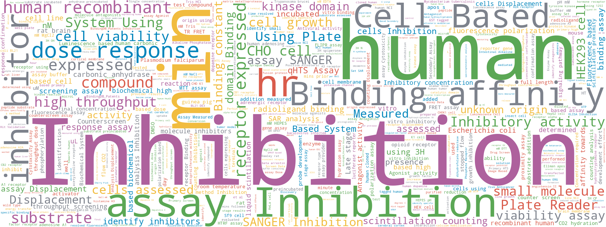
Figure A5: Wordcloud of PubChem Assay descriptions.

A.3 Metrics

In this work, we report four performance metrics, which we denote as AUROC, AP, $\Delta$AP, and $\neg$AP. AUROC is the area under the ROC curve. AP is the mean average precision, which is an approximation of the area under the precision-recall curve. $\Delta$AP additionally subtracts the base-rate, portion of positive-samples in the test-set from AP for each task. The last metric, which we dub $\neg$AP for negative-class mean average precision, is not standard, but it is very informative. It is simply the mean average precision of the negative class. That is, if the negative class is coded as 0 and the positive class is coded as 1, then NegAVGP is,

$$\neg\text{AP} =\text{AP}(1-y,1-\hat{y}),$$ (A3)

where $\hat{y}$ are the predictions and $y$ is the true label. For retrieval tasks, we use the top-$k$ accuracy as well as the enrichment-factor EF (Friesner et al., 2004). Top-$k$ accuracy measures how often the active compound is within the $k$ suggested, ranked by the method. Top-$k$% is the top-$k$ accuracy divided by the number of total choices for the method. EF normalizes top-$k$ accuracy by the score of a random choice.

Choice of main metric.

Typically AUROC is used to compare different methods (Wu et al., 2018). It measures the area under the true-positive rate vs the false-positive rate for different thresholds and can be regarded as a general sorting ability of a model. A valuable property of this metric is that a random model will produce an AUROC of 0.5. However, for imbalanced datasets, AUROC should be used with caution because it weighs the more frequent class higher (Zhao et al., 2009). In drug discovery, there is a bigger emphasis on finding active compounds which are typically rare. This is much more reflected by the Area under the Precision-Recall Curve (AUPRC) (aka PRCAUC, equiv. to AP). AP is highly dependent on the base rate of the task, and averaging over many tasks biases towards imbalanced tasks. $\Delta$AP subtracts the base-rate and for a random classifier is at 0. The metric is also adopted as the main metric in the FS-Mol benchmark (termed $\Delta$AUPRC there) (Stanley et al., 2021). Alternatively, BedROC (Truchon & Bayly, 2007) might also be used (see Tab. A8). The metric has additional parameters such as $\alpha$.

A.4 Details on Contrastive Language-Assay-Molecule Pre-training (CLAMP)

A.4.1 Molecule encoders

Programmatically we handle molecules as SMILES strings (Weininger, 1988), and convert them to different other representations from which an encoding can be generated. Several encodings of molecules were considered, which we categorize into a) fingerprint-based encoding and b) NN-based encoding. Encodings can also be combined for modeling.

Fingerprint-based.

We use the Python API of the RDKit open-source chemoinformatics software to extract fingerprints. The sparse fingerprint (FP) sprsFP is a concatenation of Daylight-like FPs, Morgan fingerprints and MACCS keys. We remove fingerprint features with low variance across training samples and finally end up with a vector of size 2176. Mc+RDKc is an addition of fingerprint-counts from the Morgan fingerprint and the RDKit-FP. We additionally scale the counts by $\ln(1+c)$.

NN-based.

We included the following NN-based embeddings, which were pre-trained in a self-supervised fashion: Grover (Rong et al., 2020), a graph transformer, CDDD (Winter et al., 2019), a SMILES-LSTM based autoencoder, MFBERT (Abdel-Aty & Gould, 2022) a SMILES-Transformer. The embeddings from these neural networks are projected by a linear layer into $d$-dimensional embeddings. Further details on the network architecture and the choice of the dimension $d$ are provided in Sec. A.4.3. Results for different embeddings can be seen in Tab. A15.

A.4.2 Assay encoders

For each unique bioassay in the bioactivity dataset, we retrieve a textual description of the bioassay, which includes both the bioassay title and, if available, a more detailed description. We process each textual description to obtain a fix-length bioassay vector. We follow two different pipelines, which we then assess separately.

Term-based.

We pre-train a Latent Semantic Analysis LSA (Deerwester et al., 1990) model on bioassay descriptions. In the case of PubChem, we obtain textual descriptions for 1,252,874 bioassays. To avoid leaking information, we exclude those corresponding to bioassays present in the validation and test splits of the bioactivity dataset. To train the LSA model, we first compute a bioassay-term matrix of tf-idf coefficients and then compute its truncated SVD decomposition. Finally, we extract the LSA embedding vectors for all the bioassay descriptions in our bioactivity dataset. The LSA embedding vectors have dimension 2048 in the case of PubChem and 128 in the case of FS-Mol. In the case of FS-Mol we additionally obtain different attributes for each assay. A collection of attributes is one-hot encoded leading to an encoding vector of size 355 termed category. A further simplistic encoding-vector in the case of FS-Mol, is a 2-dimensional vector describing if the company millipore has conducted the experiment. The FH baseline can be seen as a special case of the architecture in which a constant is used as encoding.

NN-based.

We use pre-trained model instances of several publicly available language models. We consider a BioBERT model (Lee et al., 2020), which uses a transformer architecture (Vaswani et al., 2017) and has been trained on biomedical text corpora. Each bioassay description is provided as input to BioBERT and we keep the activations at the last layer as the bioassay vector and apply mean pooling. These are of dimension 1024. We further use the text-encoder part of CLIP (Radford et al., 2021), which has been trained on a dataset of 400M image, text pairs from the internet. The output of the model is 768 dimensional. Sentence-T5 sT5 (Ni et al., 2021) is a transformer variant based on T5 (Raffel et al., 2020), trained to summarize sentences and for textual similarity. We use the XXL variant with 11b parameters available at huggingface (Jain, 2022).

A feed-forward neural network takes the assay encodings as input and projects them to $d$-dimensional embeddings. Further details on the network architecture and the choice of the dimension $d$ are provided in Sec. A.4.4. Results for different assay encodings can be seen in Tab. A14. We found a combination of LSA and CLIP to work well in our setting.

A.4.3 Feed forward neural networks

The molecule and the bioassay encoders process their input vectors using each a feed-forward neural network. The network architecture on each encoder can be different, except for the output dimensionality $d$, which maps into the shared multi-modal embedding space.

The input and hidden layers of the fully-connected networks have the following structure

$$\bm{h}^{l+1} =\text{dropout}\Big{(}\text{ReLU}\big{(}\text{norm}(\bm{W}\bm{h}^{l}+\bm{b})\big{)}\Big{)},$$ (A4)

where $\bm{h}^{l}$ is the input to the layer and $\bm{h}^{l+1}$ is its output. The variables $\bm{W}$ and $\bm{b}$ are learnable weights. The preactivations are followed by batch normalization (Ioffe & Szegedy, 2015) or layer normalization (Ba et al., 2016), a rectified linear unit (ReLU) activation function, and dropout (Srivastava et al., 2014). The output layer does not have normalization, activation function, nor dropout, as it directly serves as the molecule or the bioassay embedding.

A.4.4 Hyperparameters

Models were selected by conducting a manual hyperparameter search (Tab. A6). We explored different configurations for the embedding dimension $d$, the learning rate, the number of layers, the number of hidden units in each layer, and the dropout probability. We also experimented with the parameter $\tau$, necessary for the scoring function (Eq. 1), being set to 1 or learned, and with using either batch or layer normalization.

Table A6: Hyperparameter settings explored during model selection

Hyperparameter	Explored values
assay encoding	-, BioBERT, LSA, category, CLIP, millipore, sT5
batch_size	12, 32, 128, 256, 512, 1024, 2048, 4096, 32768
$\tau$	1.0, learned
molecule encoding	CDDD, CLIP, Graphormer, GROVER, MFBERT, Morganc+RDKc, sprsFP
dropout_hidden	0.05, 0.1, 0.15, 0.2, 0.3, 0.4
dropout_input	0.0, 0.1
embedding_size	128, 256, 512, 768, 1024, 2048
epoch_max	1, 2, 3, 4, 5, 7, 10, 50
hidden_layers	[1024, 1024], [2048, 1024], [4096, 2048, 1024], [4096, 2048], [4096, 4096, 2048], [4096], [4098, 4098], [512, 512]
lr_factor	0.95, 1.0
lr_ini	0.0001, 1e-05, 2e-05, 3e-05, 4e-05, 5e-05
model_class	Galactica, FH, KVPLM, MLPLayerNorm, MultitaskMLPLayerNorm, ScaledMLPLayerNorm
multitask_temperature	1, 100, 10e6, nan
nonlinearity	ReLU
optimizer	Adam, AdamW
patience	1, 3, 5, 10

• dropout_hidden: Dropout rate at the hidden layers

• dropout_input: Dropout rate at the input layer

• lr_factor: cosine annealing lr-schedule factor

• lr_ini: initial learning-rate

• embedding_size: association dimension $d$

• multitask_temperature: softmax temperature for 1-/soft-NN baseline

• patience: nr. of epochs to continue training after best optimization score has been reached

Table A7: Hyperparameter settings selected based on validation performance.

Hyperparameter	FSMOL				PubChem
	default				hts				time_a				time_a_c
	1-NN	CLAMP	Frequent hitters	soft-NN	1-NN	CLAMP	Frequent hitters	soft-NN	1-NN	CLAMP	Frequent hitters	soft-NN	1-NN	CLAMP	Frequent hitters	soft-NN
assay encoding	LSA	clip& lsa	-	LSA	LSA	clip& lsa&sT5	-	LSA	LSA	clip& lsa	-	clip& lsa	LSA	clip& lsa&sT5	-	clip& lsa
batch_size	512	256	512	512	512	2,048	1,024	4,096	512	1,024	512	1,024	1,024	32,768	512	512
molecule encoding	mc+rdkc	mc+rdkc	mc+rdkc	mc+rdkc	sprsFP	mc+rdkc	mc+rdkc	sprsFP	sprsFP	mc+rdkc	sprsFP	mc+rdkc	sprsFP	mc+rdkc	sprsFP	sprsFP
dropout_hidden	0.20	0.40	0.20	0.20	0.20	0.30	0.20	0.20	0.20	0.20	0.20	0.20	0.30	0.30	05	0.20
dropout_input	0	0.1	0	0	0	0.1	0.1	0	0	0.1	0	0.1	0.1	0.1	0.1	0
embedding_size	1,024	512	1,024	1,024	1,024	768	1,024	1,024	1,024	768	1,024	768	768	768	256	1,024
epoch_max	50	50	50	50	50	50	50	50	50	50	50	50	50	50	50	50
hidden_layers	[4096, 2048]	[2048, 1024]	[4096, 2048]	[4096, 2048]	[4096, 2048]	[4096, 2048]	[2048, 1024]	[4096, 2048]	[4096, 2048]	[4096, 2048, 1024]	[4096, 2048]	[4096, 2048]	[4096, 2048]	[4096, 2048]	[4096, 2048]	[4096, 2048]
layer_norm	True	True	False	True	True	True	False	True	True	True	False	True	True	True	False	True
lr_factor	1	1	1	1	1	1	1	1	1	1	1	1	1	1	1	1
lr_ini	1e-05	1e-05	1e-05	1e-05	1e-05	4e-05	5e-05	1e-05	1e-05	5e-05	1e-05	5e-05	5e-05	5e-05	5e-05	1e-05
MT_temperature	10e6	NaN	NaN	1	10e6	NaN	1	1	10e6	NaN	NaN	1	10e6	NaN	NaN	1
patience	3	3	5	3	3	3	3	3	3	3	3	3	3	3	1	3
$\tau$	1	1	1	1	1	1	1	1	1	1	1	1	1	1	1	1
warmup_epochs	2	2	0	2	2	2	2	2	2	2	2	2	2	2	1	2

• dropout_hidden: Dropout rate at the hidden layers

• dropout_input: Dropout rate at the input layer

• lr_factor: cosine annealing lr-schedule factor

• lr_ini: initial learning-rate

• embedding_size: association dimension $d$

• multitask_temperature: softmax temperature for 1-/soft-NN baseline

• patience: nr. of epochs to continue training after best optimization score has been reached

Model weights were initialized with MSRA (He et al., 2015). For each hyperparameter configuration, we optimized the objective function (Eq. 3) using AdamW (Loshchilov & Hutter, 2017). For each hyperparameter configuration, a copy of the model weights achieving the highest $\Delta AP$ on the respective validation set over max_epochs training epochs was stored. Upon analysis of the obtained validation metrics, we selected the final models (Tab. A7).

A.5 Details on compared methods and baselines

1-NN and soft-NN.

We propose baselines, which could be considered two variants of multi-task deep networks (MT-DNN), for the purpose of making activity predictions for novel bioassays. Our baselines could, however, also be considered as new methods, as, to the best of our knowledge, they have not been suggested before. In both cases, for a target novel bioassay, we compute the cosine similarity between its text encoding and those of all the training bioassays, thus obtaining a vector of textual similarities. The first baseline method, 1-nearest neighbour (1-NN), predicts the bioactivity values that MT-DNN would predict for the training bioassay most similar to the target novel bioassay. If the training set of this reference is vastly different from the molecules that should be predicted, technically predictions can be made, but they will suffer from the usual decreased performance caused by the domain shift. In this scenario also an experienced chemist might find it hard to find a reference experiment.

The second baseline, soft-nearest neighbours (soft-NN), is a smoother version of the first one. The vector of similarities between the target novel bioassay and the training bioassays is normalized using the softmax function, such that the resulting vector of weights sums up to one. Then, soft-NN predicts the weighted average of the values that MT-DNN would predict for all the training bioassays.

Frequent hitters (FH).

A further baseline is the Frequent hitters (FH) model (Schimunek et al., 2023). This baseline models the average activity of a molecule, regardless of the assay. This model can perform well because there are molecules that show up repeatedly as “active” across many different bioassays, and are also termed promiscuous molecules. Several publications have described the phenomena (Roche et al., 2002; Gilberg et al., 2016; Senger et al., 2016; Schuffenhauer et al., 2020), but it is missing as a baseline in publications related to few-and-zero-shot drug discovery (Stanley et al., 2021; Chen et al., 2022). Frequent hitter molecules can be related to molecules which interfere with the measurement rather than the object of interest, so called Pan-Assay Interference Compounds (PAINS) (Baell & Holloway, 2010; Baell & Nissink, 2018).

Hyperparameters.

We trained a dedicated MT-DNN for each baseline model. Since our training-, validation-, and test-splits are bioassay-wise disjoint, we propose the following training procedure. Each MT-DNN visits the training-set as usual, but it is then evaluated on the (bioassay-wise disjoint) validation set by using its predictions directly as 1-NN or soft-NN. In this way, we can train MT-DNN models for our baselines using exactly the same splits and information that CLAMP used.

Given the results of the hyperparameter search conducted for CLAMP, we conducted a hyperparameter search where we explored different configurations for the learning rate, the number of layers, the number of hidden units in each layer, and the dropout probability (Tab. A6). We set the parameter $\tau$ to $1$ and used layer normalization.

Model weights were initialized with MSRA (He et al., 2015). For each hyperparameter configuration, we optimized the multi-task masked loss (Mayr et al., 2016) using AdamW (Loshchilov & Hutter, 2017) with a batch size of 512 samples. For each hyperparameter configuration, a copy of the model weights achieving the highest validation $\Delta$AP over epoch_max training epochs was stored. Upon analysis of the obtained validation metrics, we selected the final models (Tab. A7).

A.6 Details on the Zero-Shot Transfer experiment (5.1)

A.6.1 Details on compared SLMs.

Galactica (GAL).

Galactica (GAL) is a SLM, trained on a large scientific corpus of papers. Among other scientific tasks, it was trained on the structure of 20M molecules, as well as on a set of 44 assays from the MoleculeNet benchmark (Wu et al., 2018). We used the publicly available weights, and test the model. Currently, only one of the specifically designed prompts is known, in order to query the model about bioassays. We design our prompt similar to the one suggested in the paper in the form of:

"Here is a SMILES formula: [START_SMILES]" + SMILES + "[END_SMILES] Will the chemical molecule be active in the assay:" + ASSAY_DESCRIPTION + "Answer (Yes or No):".

Further, we take the logit at the position of the "Yes" token as ranking between molecules.

Table A8: Zero-shot results for different metrics in %. Green values indicate the highest values and yellow values within the std to the maximum value. Error bars represent standard deviations across the best five runs based on validation $\Delta$AP.

metric	dataset	split	random	GAL 125M†	KV-PLM†	1-NN	soft-NN	FH	CLAMP
$\Delta$AP	FS-Mol	default	${01.57^{\pm{0.3}}}$	${01.44^{\pm{0.0}}}$	${01.84^{\pm{0.0}}}$	${14.68^{\pm{0.7}}}$	${13.81^{\pm{1.8}}}$	${18.50^{\pm{0.2}}}$	${19.37^{\pm{0.2}}}$
	PubChem	hts	${00.01^{\pm{0.0}}}$	${00.00^{\pm{0.0}}}$	${00.10^{\pm{0.0}}}$	${01.20^{\pm{0.1}}}$	${02.04^{\pm{0.4}}}$	${03.10^{\pm{0.1}}}$	${08.43^{\pm{0.1}}}$
		time_a	${02.13^{\pm{0.3}}}$	${01.39^{\pm{0.0}}}$	${03.57^{\pm{0.0}}}$	${12.96^{\pm{1.0}}}$	${05.67^{\pm{0.7}}}$	${10.23^{\pm{0.5}}}$	${14.77^{\pm{0.3}}}$
		time_a_c	${04.39^{\pm{0.5}}}$	${04.20^{\pm{0.0}}}$	${07.99^{\pm{0.0}}}$	${11.11^{\pm{0.3}}}$	${06.99^{\pm{2.8}}}$	${10.35^{\pm{0.9}}}$	${11.67^{\pm{0.6}}}$
AUROC	FS-Mol	default	${50.24^{\pm{0.4}}}$	${50.50^{\pm{0.0}}}$	${50.56^{\pm{0.0}}}$	${64.69^{\pm{0.8}}}$	${63.92^{\pm{1.9}}}$	${68.22^{\pm{0.2}}}$	${69.26^{\pm{0.2}}}$
	PubChem	hts	${49.92^{\pm{0.2}}}$	${49.32^{\pm{0.0}}}$	${49.65^{\pm{0.0}}}$	${67.92^{\pm{0.8}}}$	${68.41^{\pm{0.9}}}$	${73.48^{\pm{0.4}}}$	${73.83^{\pm{0.3}}}$
		time_a	${50.08^{\pm{0.5}}}$	${47.05^{\pm{0.0}}}$	${54.92^{\pm{0.0}}}$	${66.53^{\pm{0.6}}}$	${57.85^{\pm{1.7}}}$	${66.77^{\pm{1.5}}}$	${68.66^{\pm{0.5}}}$
		time_a_c	${49.91^{\pm{0.4}}}$	${48.04^{\pm{0.0}}}$	${57.00^{\pm{0.0}}}$	${61.98^{\pm{0.4}}}$	${55.06^{\pm{6.3}}}$	${61.65^{\pm{0.8}}}$	${63.66^{\pm{0.4}}}$
BEDROC	FS-Mol	default	${48.16^{\pm{0.6}}}$	${49.12^{\pm{0.0}}}$	${47.63^{\pm{0.0}}}$	${67.53^{\pm{1.0}}}$	${66.04^{\pm{2.5}}}$	${73.30^{\pm{0.5}}}$	${73.77^{\pm{0.6}}}$
	PubChem	hts	${05.31^{\pm{0.1}}}$	${05.21^{\pm{0.0}}}$	${05.96^{\pm{0.0}}}$	${18.53^{\pm{1.2}}}$	${21.37^{\pm{0.7}}}$	${27.27^{\pm{0.6}}}$	${32.02^{\pm{0.7}}}$
		time_a	${34.44^{\pm{0.8}}}$	${33.23^{\pm{0.0}}}$	${36.00^{\pm{0.0}}}$	${50.67^{\pm{1.1}}}$	${40.55^{\pm{1.3}}}$	${47.51^{\pm{0.7}}}$	${54.06^{\pm{0.7}}}$
		time_a_c	${35.18^{\pm{1.6}}}$	${35.31^{\pm{0.0}}}$	${39.16^{\pm{0.0}}}$	${43.53^{\pm{0.4}}}$	${37.06^{\pm{4.3}}}$	${42.73^{\pm{1.8}}}$	${44.81^{\pm{1.1}}}$
AP	FS-Mol	default	${48.75^{\pm{0.3}}}$	${48.48^{\pm{0.0}}}$	${49.02^{\pm{0.0}}}$	${61.86^{\pm{0.7}}}$	${60.99^{\pm{1.8}}}$	${65.68^{\pm{0.2}}}$	${66.55^{\pm{0.2}}}$
	PubChem	hts	${00.58^{\pm{0.0}}}$	${00.57^{\pm{0.0}}}$	${00.67^{\pm{0.0}}}$	${01.78^{\pm{0.1}}}$	${02.61^{\pm{0.4}}}$	${03.67^{\pm{0.1}}}$	${09.00^{\pm{0.1}}}$
		time_a	${35.42^{\pm{0.3}}}$	${34.68^{\pm{0.0}}}$	${36.87^{\pm{0.0}}}$	${46.26^{\pm{1.0}}}$	${38.97^{\pm{0.7}}}$	${43.53^{\pm{0.5}}}$	${48.06^{\pm{0.3}}}$
		time_a_c	${38.50^{\pm{0.5}}}$	${38.31^{\pm{0.0}}}$	${42.10^{\pm{0.0}}}$	${45.22^{\pm{0.3}}}$	${41.10^{\pm{2.8}}}$	${44.46^{\pm{0.9}}}$	${45.78^{\pm{0.6}}}$
$\neg$AP	FS-Mol	default	${54.17^{\pm{0.3}}}$	${54.56^{\pm{0.0}}}$	${54.38^{\pm{0.0}}}$	${67.87^{\pm{0.8}}}$	${67.24^{\pm{1.8}}}$	${71.04^{\pm{0.3}}}$	${72.22^{\pm{0.2}}}$
	PubChem	hts	${99.43^{\pm{0.0}}}$	${99.45^{\pm{0.0}}}$	${99.43^{\pm{0.0}}}$	${99.71^{\pm{0.0}}}$	${99.68^{\pm{0.0}}}$	${99.78^{\pm{0.0}}}$	${99.77^{\pm{0.0}}}$
		time_a	${69.03^{\pm{0.2}}}$	${68.27^{\pm{0.0}}}$	${71.45^{\pm{0.0}}}$	${75.30^{\pm{0.2}}}$	${73.07^{\pm{0.8}}}$	${76.24^{\pm{0.4}}}$	${76.19^{\pm{0.3}}}$
		time_a_c	${69.36^{\pm{0.1}}}$	${68.36^{\pm{0.0}}}$	${72.78^{\pm{0.0}}}$	${74.63^{\pm{0.1}}}$	${72.05^{\pm{2.1}}}$	${74.75^{\pm{0.5}}}$	${74.67^{\pm{0.5}}}$

^† for the SLMs, we chose a single model provided by the authors. Training re-runs are computationally too costly.

KV-PLM.

The SLM KV-PLM (Zeng et al., 2022b) is also able to process molecules and text in one model. KV-PLM is a BERT (Devlin et al., 2019) transformer variant and the weights, as well as the tokenizer, are available online. We use the matching score from SMILES input and textual description as ranking for molecules within an assay. As textual description, we use the same assay description source as in CLAMP (see Tab. A5 for example descriptions). KV-PLM has not been trained on assay descriptions specifically and tuning the prompt remains future work.

A.6.2 Additional metrics

Tab. A8 is an extension of Tab. 1 with additional metrics. CLAMP significantly (paired Wilcoxon test) outperforms all baselines and other methods with respect to both $\Delta$AP and AUROC. The FH method performs well for $\neg$AP for the three splits in PubChem (not significantly compared to CLAMP). We speculate, that it might have learned general attributes about molecules that make them very unlikely to be active in any assay.

A.7 Details on the representation learning study (5.2)

We examine the effectiveness of representation learning methods by evaluating the ability to produce rich representations for a variety of tasks. The quality of a learned representation is a highly debated topic in the field, but one important aspect is, that a given representation is linearly separable for a given new task (Alain & Bengio, 2016).

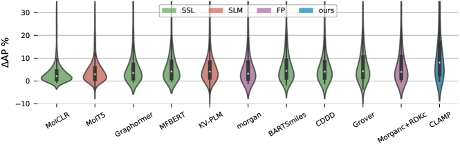
Figure A6: $\Delta AP$ violin-plot over all tasks within the downstream datasets. SSL represents self-supervised methods, SLM scientific language models, FP fingerprint baselines.

We use linear probing performance as a proxy for representation quality (Alain & Bengio, 2016; Radford et al., 2021). We precompute the representations for several methods, and run a logistic regression model for 1500 iterations with balanced class weights, L2 regularization and lbfgs solver. We compute a Logistic Regression model for each method and assay, and compute the metrics as mean performance over assays. Tab. 2 in the main manuscript shows the $\Delta$AP results and Fig. A6 shows a violin-plot representing the $\Delta$AP distribution for each method and per assay.

A.7.1 Further metrics for results

Tab. A10 is an extension of Tab. 2 with the AUROC metric. CLAMP significantly (paired Wilcoxon test) outperforms all baselines and other methods with respect to AUROC.

Table A9: Linear probing results of different methods with respect to $\Delta$AP, including Galactica. Green cells indicate the highest values in a category of tasks and areas in yellow cells within the standard deviation to the maximum value. Because of the low variability of training re-runs of a linear probing model, the error bars represent standard deviation obtained through bootstrap resampling. Rank-avg represents the mean rank over all assays. Methods are assigned to categories (cat): self-supervised learning methods (SSL), scientific language models (SLM), and chemical descriptors or fingerprints (FP)

dataset		BACE	BBBP	ClinTox	HIV	SIDER	Tox21	ToxCast	Tox21-10k
split		scaffold	scaffold	scaffold	scaffold	scaffold	scaffold	scaffold	original
# of assays	cat	1	1	2	1	27	12	617	68	rank-avg
CLAMP	ours	${27.47^{\pm{\scriptscriptstyle 4}}}$	${16.47^{\pm{\scriptscriptstyle 4}}}$	${11.05^{\pm{\scriptscriptstyle 6}}}$	${28.49^{\pm{\scriptscriptstyle 4}}}$	${08.96^{\pm{\scriptscriptstyle 4}}}$	${23.35^{\pm{\scriptscriptstyle 6}}}$	${09.44^{\pm{\scriptscriptstyle 5}}}$	${51.27^{\pm{\scriptscriptstyle 10}}}$	${02.85^{\pm{\scriptscriptstyle 2}}}$
Grover	SSL	${21.74^{\pm{\scriptscriptstyle 4}}}$	${16.76^{\pm{\scriptscriptstyle 4}}}$	${22.74^{\pm{\scriptscriptstyle 8}}}$	${13.58^{\pm{\scriptscriptstyle 3}}}$	${05.41^{\pm{\scriptscriptstyle 4}}}$	${12.88^{\pm{\scriptscriptstyle 5}}}$	${05.22^{\pm{\scriptscriptstyle 3}}}$	${42.23^{\pm{\scriptscriptstyle 10}}}$	${05.08^{\pm{\scriptscriptstyle 3}}}$
Mc+RDKc	FP	${23.87^{\pm{\scriptscriptstyle 4}}}$	${18.39^{\pm{\scriptscriptstyle 4}}}$	${17.75^{\pm{\scriptscriptstyle 7}}}$	${25.57^{\pm{\scriptscriptstyle 4}}}$	${08.43^{\pm{\scriptscriptstyle 4}}}$	${13.96^{\pm{\scriptscriptstyle 5}}}$	${05.18^{\pm{\scriptscriptstyle 4}}}$	${42.45^{\pm{\scriptscriptstyle 10}}}$	${05.64^{\pm{\scriptscriptstyle 3}}}$
CDDD	SSL	${17.51^{\pm{\scriptscriptstyle 5}}}$	${20.56^{\pm{\scriptscriptstyle 4}}}$	${33.82^{\pm{\scriptscriptstyle 7}}}$	${12.29^{\pm{\scriptscriptstyle 3}}}$	${05.30^{\pm{\scriptscriptstyle 4}}}$	${10.34^{\pm{\scriptscriptstyle 4}}}$	${04.82^{\pm{\scriptscriptstyle 3}}}$	${36.32^{\pm{\scriptscriptstyle 9}}}$	${05.79^{\pm{\scriptscriptstyle 3}}}$
BARTSmiles	SSL	${29.16^{\pm{\scriptscriptstyle 3}}}$	${17.09^{\pm{\scriptscriptstyle 4}}}$	${10.94^{\pm{\scriptscriptstyle 6}}}$	${07.88^{\pm{\scriptscriptstyle 2}}}$	${05.24^{\pm{\scriptscriptstyle 4}}}$	${10.34^{\pm{\scriptscriptstyle 4}}}$	${05.07^{\pm{\scriptscriptstyle 3}}}$	${30.40^{\pm{\scriptscriptstyle 9}}}$	${05.79^{\pm{\scriptscriptstyle 3}}}$
KV-PLM	SLM	${24.44^{\pm{\scriptscriptstyle 4}}}$	${17.61^{\pm{\scriptscriptstyle 4}}}$	${07.08^{\pm{\scriptscriptstyle 4}}}$	${06.20^{\pm{\scriptscriptstyle 2}}}$	${04.61^{\pm{\scriptscriptstyle 4}}}$	${09.90^{\pm{\scriptscriptstyle 4}}}$	${04.53^{\pm{\scriptscriptstyle 3}}}$	${30.92^{\pm{\scriptscriptstyle 10}}}$	${05.88^{\pm{\scriptscriptstyle 3}}}$
MFBERT	SSL	${14.89^{\pm{\scriptscriptstyle 4}}}$	${19.77^{\pm{\scriptscriptstyle 4}}}$	${11.84^{\pm{\scriptscriptstyle 7}}}$	${06.09^{\pm{\scriptscriptstyle 1}}}$	${06.93^{\pm{\scriptscriptstyle 4}}}$	${08.46^{\pm{\scriptscriptstyle 4}}}$	${04.72^{\pm{\scriptscriptstyle 3}}}$	${25.61^{\pm{\scriptscriptstyle 8}}}$	${06.20^{\pm{\scriptscriptstyle 3}}}$
Graphormer	SSL	${20.22^{\pm{\scriptscriptstyle 4}}}$	${08.67^{\pm{\scriptscriptstyle 4}}}$	${04.51^{\pm{\scriptscriptstyle 4}}}$	${06.87^{\pm{\scriptscriptstyle 2}}}$	${05.71^{\pm{\scriptscriptstyle 4}}}$	${08.16^{\pm{\scriptscriptstyle 4}}}$	${04.10^{\pm{\scriptscriptstyle 3}}}$	${29.50^{\pm{\scriptscriptstyle 9}}}$	${06.55^{\pm{\scriptscriptstyle 3}}}$
Morgan	FP	${27.79^{\pm{\scriptscriptstyle 4}}}$	${16.06^{\pm{\scriptscriptstyle 4}}}$	${23.86^{\pm{\scriptscriptstyle 8}}}$	${16.23^{\pm{\scriptscriptstyle 4}}}$	${06.97^{\pm{\scriptscriptstyle 4}}}$	${09.69^{\pm{\scriptscriptstyle 4}}}$	${04.28^{\pm{\scriptscriptstyle 3}}}$	${36.07^{\pm{\scriptscriptstyle 10}}}$	${06.64^{\pm{\scriptscriptstyle 3}}}$
MolT5	SLM	${11.51^{\pm{\scriptscriptstyle 4}}}$	${16.03^{\pm{\scriptscriptstyle 4}}}$	${10.06^{\pm{\scriptscriptstyle 6}}}$	${15.92^{\pm{\scriptscriptstyle 3}}}$	${02.91^{\pm{\scriptscriptstyle 3}}}$	${06.20^{\pm{\scriptscriptstyle 3}}}$	${03.53^{\pm{\scriptscriptstyle 3}}}$	${15.65^{\pm{\scriptscriptstyle 6}}}$	${07.36^{\pm{\scriptscriptstyle 3}}}$
MolCLR	SSL	${15.59^{\pm{\scriptscriptstyle 4}}}$	${13.01^{\pm{\scriptscriptstyle 4}}}$	${00.99^{\pm{\scriptscriptstyle 3}}}$	${02.57^{\pm{\scriptscriptstyle 1}}}$	${06.13^{\pm{\scriptscriptstyle 4}}}$	${06.08^{\pm{\scriptscriptstyle 3}}}$	${02.43^{\pm{\scriptscriptstyle 2}}}$	${13.21^{\pm{\scriptscriptstyle 5}}}$	${08.20^{\pm{\scriptscriptstyle 3}}}$
GAL 6.7B	SLM	${23.14^{\pm{\scriptscriptstyle 4}}}$	${24.53^{\pm{\scriptscriptstyle 4}}}$	- †	${18.35^{\pm{\scriptscriptstyle 4}}}$	-†	${13.79^{\pm{\scriptscriptstyle 5}}}$	-†	${42.80^{\pm{\scriptscriptstyle 11}}}$	-

^† model was pre-trained on a different split which would result in dataset-leakage and an overestimate in performance

Table A10: Linear probing results of different methods with respect to AUROC. Green cells indicate the highest values in a category of tasks and areas in yellow cells within the standard-deviation to the best value. Because of the low variability of training re-runs of a linear probing model, the error bars represent bootstrap standard deviation. Rank-avg represents the mean rank over all assays.

	BACE	BBBP	ClinTox	HIV	SIDER	Tox21	ToxCast	Tox21-10k
	scaffold	scaffold	scaffold	scaffold	scaffold	scaffold	scaffold	split	rank-avg
CLAMP	${84.28^{\pm{\scriptscriptstyle 3}}}$	${68.22^{\pm{\scriptscriptstyle 4}}}$	${75.31^{\pm{\scriptscriptstyle 8}}}$	${76.34^{\pm{\scriptscriptstyle 2}}}$	${65.15^{\pm{\scriptscriptstyle 7}}}$	${78.23^{\pm{\scriptscriptstyle 4}}}$	${74.00^{\pm{\scriptscriptstyle 6}}}$	${90.85^{\pm{\scriptscriptstyle 4}}}$	${02.41^{\pm{\scriptscriptstyle 2}}}$
Grover	${78.64^{\pm{\scriptscriptstyle 4}}}$	${67.94^{\pm{\scriptscriptstyle 4}}}$	${89.48^{\pm{\scriptscriptstyle 4}}}$	${77.52^{\pm{\scriptscriptstyle 2}}}$	${59.63^{\pm{\scriptscriptstyle 7}}}$	${68.16^{\pm{\scriptscriptstyle 5}}}$	${67.26^{\pm{\scriptscriptstyle 7}}}$	${86.62^{\pm{\scriptscriptstyle 5}}}$	${04.66^{\pm{\scriptscriptstyle 3}}}$
KV-PLM	${79.91^{\pm{\scriptscriptstyle 4}}}$	${69.27^{\pm{\scriptscriptstyle 4}}}$	${73.10^{\pm{\scriptscriptstyle 9}}}$	${69.76^{\pm{\scriptscriptstyle 2}}}$	${57.36^{\pm{\scriptscriptstyle 7}}}$	${64.74^{\pm{\scriptscriptstyle 5}}}$	${66.32^{\pm{\scriptscriptstyle 7}}}$	${82.16^{\pm{\scriptscriptstyle 5}}}$	${05.32^{\pm{\scriptscriptstyle 3}}}$
CDDD	${76.83^{\pm{\scriptscriptstyle 4}}}$	${72.45^{\pm{\scriptscriptstyle 4}}}$	${92.41^{\pm{\scriptscriptstyle 5}}}$	${73.87^{\pm{\scriptscriptstyle 3}}}$	${59.72^{\pm{\scriptscriptstyle 7}}}$	${68.55^{\pm{\scriptscriptstyle 5}}}$	${64.85^{\pm{\scriptscriptstyle 7}}}$	${85.66^{\pm{\scriptscriptstyle 5}}}$	${05.52^{\pm{\scriptscriptstyle 3}}}$
BARTSmiles	${83.21^{\pm{\scriptscriptstyle 3}}}$	${70.90^{\pm{\scriptscriptstyle 4}}}$	${79.30^{\pm{\scriptscriptstyle 8}}}$	${70.91^{\pm{\scriptscriptstyle 3}}}$	${57.66^{\pm{\scriptscriptstyle 7}}}$	${65.16^{\pm{\scriptscriptstyle 5}}}$	${64.98^{\pm{\scriptscriptstyle 7}}}$	${83.04^{\pm{\scriptscriptstyle 5}}}$	${05.58^{\pm{\scriptscriptstyle 3}}}$
MFBERT	${71.63^{\pm{\scriptscriptstyle 4}}}$	${71.61^{\pm{\scriptscriptstyle 3}}}$	${77.99^{\pm{\scriptscriptstyle 10}}}$	${71.12^{\pm{\scriptscriptstyle 2}}}$	${61.14^{\pm{\scriptscriptstyle 7}}}$	${63.95^{\pm{\scriptscriptstyle 5}}}$	${63.72^{\pm{\scriptscriptstyle 7}}}$	${80.62^{\pm{\scriptscriptstyle 5}}}$	${06.13^{\pm{\scriptscriptstyle 3}}}$
Graphormer	${75.72^{\pm{\scriptscriptstyle 4}}}$	${58.71^{\pm{\scriptscriptstyle 4}}}$	${68.64^{\pm{\scriptscriptstyle 9}}}$	${71.61^{\pm{\scriptscriptstyle 3}}}$	${58.82^{\pm{\scriptscriptstyle 7}}}$	${65.48^{\pm{\scriptscriptstyle 5}}}$	${62.92^{\pm{\scriptscriptstyle 7}}}$	${83.38^{\pm{\scriptscriptstyle 5}}}$	${06.38^{\pm{\scriptscriptstyle 3}}}$
MolT5	${63.46^{\pm{\scriptscriptstyle 5}}}$	${65.06^{\pm{\scriptscriptstyle 4}}}$	${73.78^{\pm{\scriptscriptstyle 9}}}$	${72.81^{\pm{\scriptscriptstyle 3}}}$	${53.20^{\pm{\scriptscriptstyle 7}}}$	${63.63^{\pm{\scriptscriptstyle 4}}}$	${62.98^{\pm{\scriptscriptstyle 7}}}$	${74.99^{\pm{\scriptscriptstyle 6}}}$	${06.88^{\pm{\scriptscriptstyle 3}}}$
Mc+RDKc	${81.16^{\pm{\scriptscriptstyle 4}}}$	${69.67^{\pm{\scriptscriptstyle 4}}}$	${84.81^{\pm{\scriptscriptstyle 5}}}$	${72.25^{\pm{\scriptscriptstyle 3}}}$	${62.41^{\pm{\scriptscriptstyle 7}}}$	${69.61^{\pm{\scriptscriptstyle 5}}}$	${60.73^{\pm{\scriptscriptstyle 8}}}$	${82.72^{\pm{\scriptscriptstyle 6}}}$	${06.99^{\pm{\scriptscriptstyle 3}}}$
Morgan	${80.94^{\pm{\scriptscriptstyle 3}}}$	${66.09^{\pm{\scriptscriptstyle 4}}}$	${74.99^{\pm{\scriptscriptstyle 9}}}$	${71.31^{\pm{\scriptscriptstyle 3}}}$	${59.00^{\pm{\scriptscriptstyle 7}}}$	${64.65^{\pm{\scriptscriptstyle 5}}}$	${59.12^{\pm{\scriptscriptstyle 8}}}$	${79.99^{\pm{\scriptscriptstyle 6}}}$	${07.98^{\pm{\scriptscriptstyle 3}}}$
MolCLR	${70.43^{\pm{\scriptscriptstyle 5}}}$	${61.07^{\pm{\scriptscriptstyle 4}}}$	${53.64^{\pm{\scriptscriptstyle 12}}}$	${63.87^{\pm{\scriptscriptstyle 3}}}$	${56.84^{\pm{\scriptscriptstyle 7}}}$	${63.16^{\pm{\scriptscriptstyle 4}}}$	${59.23^{\pm{\scriptscriptstyle 7}}}$	${73.82^{\pm{\scriptscriptstyle 6}}}$	${08.16^{\pm{\scriptscriptstyle 3}}}$
Gal 6.7B	${78.97^{\pm{\scriptscriptstyle 4}}}$	${75.72^{\pm{\scriptscriptstyle 3}}}$	-	${74.10^{\pm{\scriptscriptstyle 3}}}$	-	${69.14^{\pm{\scriptscriptstyle 5}}}$	-	${86.84^{\pm{\scriptscriptstyle 5}}}$	-

A.7.2 Comparison to literature.

In this section, we present a selection of prior works that have also benchmarked on the MoleculeNet dataset. For a fair comparison, is important to ensure that the same data split in referenced prior works is also the one used in our experiments. We use the initial scaffold-split from MoleculeNet and do not take multiple-scaffold splits as in e.g. Graphormer(Ying et al., 2021). Furthermore, while many of the prior works report results using the AUROC metric, we prefer $\Delta$AP. In our experiments optimize on validation $\Delta$AP as the primary metric (Sec. A.3). Tab. A11 shows our linear probing results compared to fine-tuned models from the literature. CLAMP yields the best performance of the linear probing methods.

Table A11: MoleculeNet ROC-AUC comparison to literature reported values on scaffold-split for all datasets. LP stands for linear probing, all other methods have been fine-tuned. Standard-Error for methods with LP reports dataset bootstrap variance whereby other methods typically report re-run variance. Results are reported in % and methods are sorted by the last column.

method	LP	BACE	BBBP	ClinTox	HIV	SIDER	Tox21	Toxcast	avg
MolCLR (Wang et al., 2021b)	X	${70.43^{\pm{4.6}}}$	${61.07^{\pm{3.9}}}$	${53.64^{\pm{11.7}}}$	${63.87^{\pm{2.6}}}$	${56.84^{\pm{7.6}}}$	${63.16^{\pm{4.6}}}$	${59.23^{\pm{8.8}}}$	${61.18^{\pm{5.0}}}$
JOAOv2 (Wang et al., 2022)		${67.40^{\pm{0.7}}}$	${66.40^{\pm{0.9}}}$	${64.50^{\pm{0.9}}}$	${68.40^{\pm{0.5}}}$	${59.10^{\pm{0.7}}}$	${68.20^{\pm{0.8}}}$	${57.00^{\pm{0.5}}}$	${64.43^{\pm{4.2}}}$
MolT5-large (Edwards et al., 2022)	X	${63.46^{\pm{4.6}}}$	${65.06^{\pm{3.9}}}$	${73.78^{\pm{8.6}}}$	${72.81^{\pm{2.7}}}$	${53.20^{\pm{7.4}}}$	${63.63^{\pm{4.4}}}$	${62.98^{\pm{8.5}}}$	${64.99^{\pm{6.4}}}$
Graphormer (Ying et al., 2021)	X	${75.72^{\pm{4.1}}}$	${58.71^{\pm{3.9}}}$	${68.64^{\pm{9.4}}}$	${71.61^{\pm{2.5}}}$	${58.82^{\pm{7.1}}}$	${65.48^{\pm{4.9}}}$	${62.92^{\pm{8.3}}}$	${65.99^{\pm{5.9}}}$
GAL 120B (Taylor et al., 2022)		${61.70^{\pm{0.0}}}$	${66.10^{\pm{0.0}}}$	${-}$	${74.50^{\pm{0.0}}}$	${-}$	${68.90^{\pm{0.0}}}$	${-}$	${67.80^{\pm{4.6}}}$
GNN (Wang et al., 2022)		${80.90^{\pm{1.9}}}$	${66.40^{\pm{0.9}}}$	${66.30^{\pm{0.6}}}$	${71.40^{\pm{1.2}}}$	${61.70^{\pm{1.9}}}$	${69.70^{\pm{2.3}}}$	${58.70^{\pm{0.5}}}$	${67.87^{\pm{6.7}}}$
Morgan-FP	X	${80.94^{\pm{3.5}}}$	${66.09^{\pm{3.8}}}$	${74.99^{\pm{9.5}}}$	${71.31^{\pm{2.7}}}$	${59.00^{\pm{8.0}}}$	${64.65^{\pm{4.9}}}$	${59.12^{\pm{8.9}}}$	${68.01^{\pm{7.6}}}$
3D Infomax (Stärk et al., 2022)		${79.42^{\pm{1.9}}}$	${69.10^{\pm{1.1}}}$	${59.43^{\pm{3.2}}}$	${76.08^{\pm{1.3}}}$	${53.37^{\pm{3.3}}}$	${74.46^{\pm{0.7}}}$	${64.41^{\pm{0.9}}}$	${68.04^{\pm{8.8}}}$
KV-PLM (Zeng et al., 2022b)	X	${79.91^{\pm{3.8}}}$	${69.27^{\pm{3.6}}}$	${73.10^{\pm{9.4}}}$	${69.76^{\pm{2.4}}}$	${57.36^{\pm{7.4}}}$	${64.74^{\pm{5.0}}}$	${66.32^{\pm{8.1}}}$	${68.64^{\pm{6.5}}}$
MFBERT (Abdel-Aty & Gould, 2022)	X	${71.63^{\pm{4.4}}}$	${71.61^{\pm{3.3}}}$	${77.99^{\pm{10.2}}}$	${71.12^{\pm{2.4}}}$	${61.14^{\pm{7.4}}}$	${63.95^{\pm{4.8}}}$	${63.72^{\pm{8.3}}}$	${68.74^{\pm{5.5}}}$
MISU (Benjamin et al., 2022)		${70.52^{\pm{3.8}}}$	${66.71^{\pm{1.8}}}$	${78.00^{\pm{4.3}}}$	${-}$	${59.73^{\pm{0.8}}}$	${76.30^{\pm{0.7}}}$	${62.79^{\pm{0.5}}}$	${69.01^{\pm{6.7}}}$
KV-PLM (Zeng et al., 2022b)		${78.50^{\pm{2.7}}}$	${70.50^{\pm{0.5}}}$	${89.17^{\pm{2.7}}}$	${65.40^{\pm{1.7}}}$	${59.83^{\pm{0.6}}}$	${72.12^{\pm{1.0}}}$	${55.03^{\pm{1.6}}}$	${70.08^{\pm{10.6}}}$
BARTSmiles (Chilingaryan et al., 2022)	X	${83.21^{\pm{3.3}}}$	${70.90^{\pm{3.7}}}$	${79.30^{\pm{7.5}}}$	${70.91^{\pm{2.6}}}$	${57.66^{\pm{6.9}}}$	${65.16^{\pm{5.0}}}$	${64.98^{\pm{8.6}}}$	${70.30^{\pm{8.1}}}$
MegaMolBART (Liu et al., 2022a)		${82.46^{\pm{0.8}}}$	${68.89^{\pm{0.2}}}$	${78.12^{\pm{4.6}}}$	${71.04^{\pm{1.7}}}$	${59.52^{\pm{1.8}}}$	${73.89^{\pm{0.7}}}$	${63.32^{\pm{0.8}}}$	${71.03^{\pm{7.4}}}$
Mc+RDKc-FP	X	${81.16^{\pm{3.5}}}$	${69.67^{\pm{3.7}}}$	${84.81^{\pm{4.9}}}$	${72.25^{\pm{2.8}}}$	${62.41^{\pm{7.7}}}$	${69.61^{\pm{4.8}}}$	${60.73^{\pm{8.9}}}$	${71.52^{\pm{8.2}}}$
Grover (Rong et al., 2020)r	X	${78.64^{\pm{3.8}}}$	${67.94^{\pm{4.0}}}$	${89.48^{\pm{4.3}}}$	${77.52^{\pm{2.2}}}$	${59.63^{\pm{7.8}}}$	${68.16^{\pm{5.4}}}$	${67.26^{\pm{8.2}}}$	${72.66^{\pm{9.1}}}$
CDDD (Winter et al., 2019)	X	${76.83^{\pm{4.2}}}$	${72.45^{\pm{3.6}}}$	${92.41^{\pm{4.6}}}$	${73.87^{\pm{2.6}}}$	${59.72^{\pm{7.1}}}$	${68.55^{\pm{5.0}}}$	${64.85^{\pm{8.2}}}$	${72.67^{\pm{9.7}}}$
GraphMVP-C (Liu et al., 2022a)		${81.20^{\pm{0.9}}}$	${72.40^{\pm{1.6}}}$	${77.50^{\pm{4.2}}}$	${77.00^{\pm{1.2}}}$	${63.90^{\pm{1.2}}}$	${74.40^{\pm{0.2}}}$	${63.10^{\pm{0.4}}}$	${72.79^{\pm{6.4}}}$
GIN-node-pretrain (Sun, 2022)		${83.66^{\pm{0.8}}}$	${73.45^{\pm{0.3}}}$	${-}$	${-}$	${65.08^{\pm{0.1}}}$	${75.30^{\pm{0.4}}}$	${66.50^{\pm{0.1}}}$	${72.80^{\pm{6.7}}}$
ECFP6||RDKd-FP	X	${80.36^{\pm{0.0}}}$	${71.98^{\pm{0.0}}}$	${87.59^{\pm{0.0}}}$	${73.45^{\pm{0.0}}}$	${63.02^{\pm{0.0}}}$	${71.41^{\pm{0.0}}}$	${67.73^{\pm{0.0}}}$	${73.65^{\pm{7.5}}}$
MOCO (Zhu et al., 2022b)		${82.60^{\pm{0.3}}}$	${71.60^{\pm{1.0}}}$	${81.60^{\pm{3.7}}}$	${78.30^{\pm{0.4}}}$	${61.20^{\pm{0.6}}}$	${76.70^{\pm{0.4}}}$	${64.90^{\pm{0.8}}}$	${73.84^{\pm{7.7}}}$
GIN-sup.-cont.-pt. (Sun, 2022)		${86.33^{\pm{0.2}}}$	${74.38^{\pm{0.9}}}$	${-}$	${-}$	${62.22^{\pm{0.5}}}$	${78.16^{\pm{0.2}}}$	${68.71^{\pm{0.1}}}$	${73.96^{\pm{8.2}}}$
MoleculeSTM-s (Liu et al., 2022a)		${81.99^{\pm{0.4}}}$	${70.75^{\pm{1.9}}}$	${86.60^{\pm{2.3}}}$	${77.02^{\pm{0.4}}}$	${63.70^{\pm{0.8}}}$	${75.71^{\pm{0.9}}}$	${65.17^{\pm{0.4}}}$	${74.42^{\pm{7.8}}}$
CLAMP	X	${84.28^{\pm{3.4}}}$	${68.22^{\pm{3.8}}}$	${75.31^{\pm{7.8}}}$	${76.34^{\pm{2.4}}}$	${65.15^{\pm{7.5}}}$	${78.23^{\pm{4.2}}}$	${74.00^{\pm{7.7}}}$	${74.50^{\pm{5.9}}}$
MoleculeSTM-g (Liu et al., 2022a)		${80.77^{\pm{1.3}}}$	${69.98^{\pm{0.5}}}$	${92.53^{\pm{1.1}}}$	${76.93^{\pm{1.8}}}$	${60.96^{\pm{1.1}}}$	${76.91^{\pm{0.5}}}$	${65.05^{\pm{0.4}}}$	${74.73^{\pm{9.8}}}$
GEM (Fang et al., 2022)		${85.60^{\pm{1.1}}}$	${72.40^{\pm{0.4}}}$	${90.10^{\pm{1.3}}}$	${-}$	${67.20^{\pm{0.4}}}$	${78.10^{\pm{0.1}}}$	${69.20^{\pm{0.4}}}$	${77.10^{\pm{8.4}}}$
Uni-Mol (Zhou et al., 2022)		${85.70^{\pm{0.2}}}$	${72.90^{\pm{0.6}}}$	${91.90^{\pm{1.8}}}$	${80.80^{\pm{0.3}}}$	${65.90^{\pm{1.3}}}$	${79.60^{\pm{0.5}}}$	${69.60^{\pm{0.1}}}$	${78.06^{\pm{8.5}}}$
MMM (He et al., 2022)		${86.20^{\pm{2.3}}}$	${75.20^{\pm{0.7}}}$	${90.90^{\pm{2.5}}}$	${-}$	${68.20^{\pm{0.4}}}$	${79.30^{\pm{0.2}}}$	${69.90^{\pm{0.2}}}$	${78.28^{\pm{8.2}}}$
Unified2D3D (Zhu et al., 2022a)		${86.80^{\pm{0.6}}}$	${77.40^{\pm{0.6}}}$	${95.40^{\pm{1.1}}}$	${82.20^{\pm{1.0}}}$	${67.40^{\pm{0.5}}}$	${75.90^{\pm{0.3}}}$	${-}$	${80.85^{\pm{8.8}}}$

A.8 Details on the retrieval and library design study (5.3)

In this task, molecules from a chemical database must be ranked according to a description of a specific bioassay. Molecules that have been measured as active in the given bioassay should be given a high ranking. If the top-k ranked molecules contain the known active, then the prediction is considered accurate. This task is a proxy for how relevant suggestions of a given method are.

We use the PubChem dataset with assay-based temporal split time_a for molecule retrieval. We consider two different set-sizes: 1M an 10k molecules, selected in order of their PubChem Compound-ID (CID). The 10k molecule setting is used for computational feasibility and to include Galactica in the comparison. To obtain robust estimates of the performance metric, we report the average over assays with more than 100 active molecules. This results in 190 assays for the 10k molecules setting and 2,543 assays for the 1M molecule setting for testing.

The enrichment-factor (EF) is used as evaluation metric (see Sec. A.3 for details). The results of this study in terms of enrichment factor for different top-$k$ accuracies are shown in Fig. A7.

Figure A7: Molecule-retrieval enrichment factor plots. The x-axis displays different $k$ for top-$k$ accuracies and on the y-axis the enrichment factor is displayed. Different methods are represented by colored lines. Each dot represents a mean over bioassays and the shaded areas indicate the standard deviation over assays. Left: Retrieving from a database of 10k molecules. Right: Retrieval from a database of 1M molecules.

A.9 Extended experiments

A.9.1 Out-of-domain zero-shot on downstream datasets.

In this experiment, we evaluate the generalization capabilities of a model in an out-of-domain setting by assessing its robustness to variations in assay description. We aim to test the model’s ability to perform well on unseen assay descriptions that are distinct from those in the training dataset.

Datasets. The MoleculeNet datasets and Tox21-10k were utilized in this study in a zero-shot manner. The original datasets did not include assay descriptions, thus, we manually created descriptions by integrating information from multiple sources. However, additional efforts are required to refine and optimize these descriptions. The zero-shot performance is evaluated on the default scaffold test-split, except for Tox21-10k where we use the default test split.

Methods compaired. We pre-train a CLAMP and FH model on PubChem, removing compounds that are in the test set (as in experiments Sec. 5.2 and further described in Sec. A.2.4), and train on a random-split. We benchmark against FH and KV-PLM. Galactica was not included as a comparison model in this study, as the use of pre-trained models on the datasets being tested would introduce a potential source of dataset leakage and lead to an overestimation of performance.

Results. Results are presented in Tab. A12. Overall, our model demonstrates prominent performance on the HIV dataset, with an AUROC score that surpasses that of linear probing performance. The performance of the FH model on the HIV dataset is also noteworthy, with an AUROC score of 68.21, which is outperformed by CLAMP with an AUROC of 80.67. The zero-shot performance, in this case, is better than the linear-probing performance of 76.34 (see Tab. A10). However, for datasets such as ClinTox and BBBP, the performance of all three models is relatively poor. On average, over datasets, our model outperforms both FH and KV-PLM.

Table A12: Out of domain zero-shot on downstream datasets. Results are reported in %. Avg represents the mean over datasets.

metric	method	BACE	BBBP	ClinTox	HIV	SIDER	Tox21	ToxCast	Tox21-10k	avg
$\Delta$AP	KVPLM	${-4.15}$	${08.63}$	${04.54}$	${00.00}$	${01.67}$	${03.20}$	${02.61}$	${04.20}$	${02.59}$
	FH	${10.78}$	${06.15}$	${01.38}$	${02.89}$	${00.32}$	${01.70}$	${03.66}$	${07.67}$	${04.32}$
	CLAMP	${07.85}$	${-0.12}$	${03.93}$	${16.24}$	${03.99}$	${05.40}$	${02.80}$	${12.02}$	${06.51}$
AUROC	KVPLM	${45.29}$	${56.38}$	${49.94}$	${53.37}$	${47.71}$	${55.73}$	${59.07}$	${60.62}$	${53.51}$
	FH	${63.77}$	${56.34}$	${48.03}$	${68.21}$	${49.14}$	${57.15}$	${61.99}$	${71.39}$	${59.50}$
	CLAMP	${64.76}$	${47.88}$	${49.03}$	${80.67}$	${54.23}$	${60.58}$	${53.83}$	${69.70}$	${60.09}$

A.9.2 Comparison to bioactivity descriptors

In this experiment, we benchmark learned representation against bioactivity descriptors. A molecule can be described structurally via e.g. a fingerprint but also assay-measurements can be used to represent a molecule. The HTS Fingerprint (HTSFP) Petrone et al. (2012) is a bioactivity descriptor using historical activity data to represent a molecules. The HTSFP has the benefit of not requiring any structural information. Additionally, active substances with distinctive mechanisms of action can be found using HTSFPs. However, predictions can only be made for substances that have already been examined in HTS assays, and substances with sparse HTSFPs are frequently removed from the dataset because they may introduce noise into the data and reduce predictive performance.

Datasets. We reproduce the setting of Laufkötter et al. (2019): 582 HTS assays from PubChem are selected, 24 of which are used for testing. The split is termed hts-split. Note that this corresponds to a random assay-split.

Methods compared. Laufkötter et al. (2019) suggests the bioactivity-structure hybrid (BaSH) fingerprint. BaSH concatenates HTSFP and a structural FP. They empirically show that the BaSH fingerprint improves performance when compared to the use of the HTSFP fingerprint alone. Compared to the implementation of Laufkötter et al. (2019), we remove all test and validation assays from the FPs and do not remove only one assay dimension at a time, when testing (leaf-one-out at the task level). Instead of using a Random Forest Model, we train a Logistic Regression model on the FPs, which corresponds to linear probing.

We compare against our method CLAMP: We pre-train a CLAMP model on training assays from the hts-split. For BaSH and HTSFP, missing values get imputed as zeros, which is not the case for our pre-training our method. We select the best model based on zero-shot validation $\Delta$AP. Finally, we test the molecular representations on the 24 test-set assays of the hts-split. We perform linear probing for each method for a 5-fold random cross-validation for each test-assays.

Results. We report the mean 5-fold cross-validation-AUROC over 24 test assays. Tab. A13 demonstrated that CLAMP outperforms the proposed BaSH fingerprint. The FH baseline is superior to using LP on fingerprint-based molecular descriptors. With only 1.23 % of training data in the pretraining set, CLAMP 2048-Shot achieves better results than HTSFP. CLAMP also addresses its drawbacks. Particularly, the BaSH and HTSFP fingerprint are restricted to molecules with activity data, whereas CLAMP can perform inference on molecules without activity data.

Table A13: Linear probing %AUROC results for PubChem hts-split. Average over 24 assays. LP stands for linear probing. % of train corresponds to the amount of training data that has been used.

method	LP	AUROC	% of train
CLAMP	x	${81.00^{\pm{3.7}}}$	$100.00$
BaSH (Laufkötter et al., 2019)	x	${79.19^{\pm{4.6}}}$	$100.00$
CLAMP 2048-Shot	x	${78.08}^{\pm{4.1}}$	$1.23$
HTSFP (Laufkötter et al., 2019)	x	${77.37^{\pm{4.0}}}$	$100.00$
CLAMP Zero-Shot		${73.84}^{\pm{4.7}}$	$0.00$
FH Zero-Shot		${73.48}^{\pm{4.8}}$	$0.00$
ECFP+TT+MACCS	x	${73.04^{\pm{5.0}}}$	$100.00$
ECFP4	x	${71.67^{\pm{4.6}}}$	$100.00$

A.9.3 Few-Shot on FS-Mol

Few-shot learning is a setting where only a number of training samples are given, the so-called support-set. The support-set can be used to train the model. The model is evaluated on the remaining samples. A support-set-size of 16 is a common choice, also referred to as 16-shot. The zero-shot setting refers to having no support-set molecules, and is particularly challenging. Specific methods have been suggested for few-shot learning for molecules (Stanley et al., 2021; Schimunek et al., 2023; Altae-Tran et al., 2017; Guo et al., 2021; Wang et al., 2021a; Chen et al., 2022). Schemes include data-augmentation-based approaches, nearest-neighbor approaches and optimization-based or fine-tuning-based methods using meta-optimizers. We don’t employ any of those techniques, and add the support-set to the pre-training set. We do this for CLAMP and FH.

Datasets. We use the same setup as in FS-Mol (Stanley et al., 2021): the data is split into a training-, validation- and test-set based on assays. We use the same split and draw a random sample of support-set-size number of molecules from the test set.

Results. Our results can be seen in Figure A8. The FH method also introduced in (Schimunek et al., 2023), provides a strong baseline, outperforming other methods like Random-Forest (RF) of few-shot specific methods like GNN-MAML(Stanley et al., 2021) even without a support-set. CLAMP shows impressive zero-and 16-shot performance, but for larger support-set-sizes is outperformed by PN(Stanley et al., 2021) and MHNfs (Schimunek et al., 2023) at 16-shot.

Specific few-shot learning schemes could also be employed on top of the CLAMP representation, which we leaf to future work.

Figure A8: Few- and Zero-shot results for FS-Mol (Stanley et al., 2021)

A.9.4 Molecule- and assay-encoder ablation

In this study, we investigated which molecule and text encoder provide the best predictive performance for the CLAMP approach. The setting is the same as in the zero-shot transfer experiments. The experiments were in no way exhaustive. We mainly explored parameters for FS-Mol due to the smaller size. Tab. A14 shows test-set performance for different assay encoders. CLIP concatenated with LSA encoding works well. Tab. A15 shows test-set performance for different molecule encoders.

Table A14: Results for different assay encodings.

assay encoding	FSMOL	PubChem
	default	hts	time_a	time_a_c
CLIP||LSA	${19.60^{\pm{0.4}}}$	${07.92^{\pm{0.8}}}$	${14.83^{\pm{0.3}}}$	${10.82^{\pm{1.6}}}$
LSA	${19.56^{\pm{0.3}}}$	${07.99^{\pm{1.3}}}$	${13.37^{\pm{1.1}}}$	${11.28^{\pm{0.8}}}$
CLIP	${19.42^{\pm{0.2}}}$		${12.72^{\pm{1.4}}}$
CLIP||LSA||sT5	${19.29^{\pm{0.5}}}$	${08.24^{\pm{0.3}}}$		${11.95^{\pm{1.4}}}$
category	${19.15^{\pm{0.2}}}$
category||millipore	${19.12^{\pm{0.3}}}$
millipore	${19.07^{\pm{0.5}}}$
BioBERT	${19.01^{\pm{0.1}}}$
constant†	${18.50^{\pm{0.2}}}$	${03.10^{\pm{0.1}}}$	${10.23^{\pm{0.5}}}$	${10.35^{\pm{0.9}}}$
GAL 6.7B	${18.50^{\pm{0.2}}}$

^† a constant as assay-encoding corresponds to FH model

Table A15: Results for different molecule encodings.

molecule encoding	FSMOL	PubChem
	default	hts	time_a	time_a_c
multiple†	${19.51^{\pm{0.2}}}$
Morganc+RDKc	${19.35^{\pm{0.2}}}$	${08.35^{\pm{0.3}}}$	${14.77^{\pm{0.3}}}$	${11.80^{\pm{0.7}}}$
CDDD	${18.17^{\pm{1.1}}}$
MFBERT	${18.43^{\pm{1.2}}}$
Grover	${17.86^{\pm{1.1}}}$
sprsFP	${13.98^{\pm{0.6}}}$	${04.14^{\pm{3.6}}}$	${11.28^{\pm{1.3}}}$	${11.18^{\pm{0.8}}}$
MolT5-large	${16.20^{\pm{2.1}}}$
KV-PLM	${11.11^{\pm{3.2}}}$
GAL 6.7B	${09.25^{\pm{0.9}}}$

^† concatenation of CDDD, Graphormer, Grover, MFBERT, Mc+RDKc.

A.10 Computational Resources

The code was run on different servers with diverse Nvidia GPUs, the best of which was an NVIDIA A100-SXM4-80GB, using PyTorch 1.13.0 (Paszke et al., 2019). The total compute run-time was around 170 days and $\sim$800 runs (without linear probing). The minimum GPU-memory experiments were run with 12GB. Further statement on computational feasibility: Based on our current setup, we would consider an experiment that is 10 times larger than our current setup as computationally infeasible.

A.11 Broader Impact

We envision that our approach can also be used to enhance models in other application domains with an interface with human language. Furthermore, our results reveal drawbacks of multi-modal language models. Our results also hint at the fact that specialized modules for each data modality whose representations are later combined could be necessary for good predictive performance.

A.12 Social Impact

Our method has the potential to significantly impact the field of drug discovery and development. By associating molecules with bioassay descriptions, the model can aid in the identification of new drug candidates and provide insight into the potential side effects of existing molecules. This can lead to a more efficient drug development process, potentially reducing time and cost associated with bringing new treatments to market.

However, it is important to note that there are also ethical and societal implications of the CLAMP method. Potential biases in the data influence the model’s predictions and highlight the need for responsible data management practices. Additionally, it is important to consider the impact of the technology and take steps to ensure that the benefits of the model are shared equitably. As previously demonstrated by Urbina et al. (2022), models like CLAMP can not only be used to identify and avoid toxicity but also to suggest highly toxic chemicals.

In conclusion, the CLAMP method has the potential to significantly impact the field of drug discovery and development, but it is crucial to consider the ethical and societal implications of the technology in order to ensure that its benefits are shared equitably. Note that our method would not be used by the general public but by researchers, such as chemists or molecular biologists.

A.13 List of Acronyms

AUPR

Area Under Precision Recall curve

AUROC

Area Under Receiver-Operating-Characterstic curve

AP

Average Precision

CV

Computer Vision

CLIP

Contrastive Language–Image Pre-training

CLAMP

Contrastive Language–Assay-Molecule Pre-training

ChEMBL

A biochemical database

ChEBI

Chemical Entities of Biological Interest

ConVIRT

Contrastive VIsual Representation Learning from Text

DL

Deep Learning

DNN

Deep Neural Network

ECFP

Extended Connectivity Fingerprint

EF

Enrichment Factor

FP

FingerPrint

FH

Frequent Hitters

GNN

Graph Neural Network

HTS

High-Throughput Screening

IUPAC

International Union of Pure and Applied Chemistry

InChI

International Chemical Identifier

KV-PLM

A scientific language model

LSA

Latent Semantic Analysis

ML

Machine Learning

NCE

Noise Contrastive Estimation

NLP

Natural Language Processing

NN

Neural Network

PubChem

A biochemical database

SLM

Scientific Language Model

SMILES

Simplified Molecular-Input Line-Entry System

References

- Abdel-Aty & Gould (2022) Abdel-Aty, H. and Gould, I. R. Large-scale distributed training of transformers for chemical fingerprinting. Journal of Chemical Information and Modeling, 62(20):4852–4862, 2022.
- Ain et al. (2015) Ain, Q. U., Aleksandrova, A., Roessler, F. D., and Ballester, P. J. Machine-learning scoring functions to improve structure-based binding affinity prediction and virtual screening. Wiley Interdisciplinary Reviews: Computational Molecular Science, 5(6):405–424, 2015.
- Alain & Bengio (2016) Alain, G. and Bengio, Y. Understanding intermediate layers using linear classifier probes. arXiv preprint arXiv:1610.01644, 2016.
- Altae-Tran et al. (2017) Altae-Tran, H., Ramsundar, B., Pappu, A. S., and Pande, V. Low data drug discovery with one-shot learning. ACS Central Science, 3(4):283–293, 2017.
- Artemov et al. (2016) Artemov, A. V., Putin, E., Vanhaelen, Q., Aliper, A., Ozerov, I. V., and Zhavoronkov, A. Integrated deep learned transcriptomic and structure-based predictor of clinical trials outcomes. BioRxiv, pp. 095653, 2016.
- Ba et al. (2016) Ba, J. L., Kiros, J. R., and Hinton, G. E. Layer normalization. arXiv preprint arXiv:1607.06450, 2016.
- Baell & Holloway (2010) Baell, J. B. and Holloway, G. A. New Substructure Filters for Removal of Pan Assay Interference Compounds (PAINS) from Screening Libraries and for Their Exclusion in Bioassays. Journal of Medicinal Chemistry, 53(7):2719–2740, 2010. ISSN 0022-2623.
- Baell & Nissink (2018) Baell, J. B. and Nissink, J. W. M. Seven Year Itch: Pan-Assay Interference Compounds (PAINS) in 2017—Utility and Limitations. ACS Chem. Biol., 13(1):36–44, 2018. ISSN 1554-8929.
- Beltagy et al. (2019) Beltagy, I., Lo, K., and Cohan, A. SciBERT: A pretrained language model for scientific text. In Proceedings of the 2019 Conference on Empirical Methods in Natural Language Processing, pp. 3615–3620, 2019.
- Bemis & Murcko (1996) Bemis, G. W. and Murcko, M. A. The properties of known drugs. 1. molecular frameworks. Journal of Medicinal Chemistry, 39(15):2887–2893, 1996.
- Bender & Cortés-Ciriano (2021) Bender, A. and Cortés-Ciriano, I. Artificial intelligence in drug discovery: what is realistic, what are illusions? part 1: ways to make an impact, and why we are not there yet. Drug Discovery Today, 26(2):511–524, 2021.
- Benjamin et al. (2022) Benjamin, R., Singer, U., and Radinsky, K. Graph neural networks pretraining through inherent supervision for molecular property prediction. In Proceedings of the 31st ACM International Conference on Information & Knowledge Management, pp. 2903–2912, 2022.
- Borgeaud et al. (2022) Borgeaud, S., Mensch, A., Hoffmann, J., Cai, T., Rutherford, E., Millican, K., Van Den Driessche, G. B., Lespiau, J.-B., Damoc, B., Clark, A., et al. Improving language models by retrieving from trillions of tokens. In International Conference on Machine Learning, pp. 2206–2240. PMLR, 2022.
- Brown et al. (2020) Brown, T., Mann, B., Ryder, N., Subbiah, M., Kaplan, J. D., Dhariwal, P., Neelakantan, A., Shyam, P., Sastry, G., Askell, A., et al. Language models are few-shot learners. Advances in Neural Information Processing Systems, 33:1877–1901, 2020.
- Chang & Ye (2022) Chang, J. and Ye, J. C. Molecular structure-property co-trained foundation model for in silico chemistry. arXiv preprint arXiv:2211.10590, 2022.
- Chang et al. (2008) Chang, M.-W., Ratinov, L., Roth, D., and Srikumar, V. Importance of semantic representation: dataless classification. In Proceedings of the 23rd National Conference on Artificial Intelligence-Volume 2, pp. 830–835, 2008.
- Chen et al. (2018) Chen, H., Engkvist, O., Wang, Y., Olivecrona, M., and Blaschke, T. The rise of deep learning in drug discovery. Drug Discovery Today, 23(6):1241–1250, 2018.
- Chen et al. (2020) Chen, T., Kornblith, S., Norouzi, M., and Hinton, G. A simple framework for contrastive learning of visual representations. In International Conference on Machine Learning, pp. 1597–1607. PMLR, 2020.
- Chen et al. (2022) Chen, W., Tripp, A., and Hernández-Lobato, J. M. Meta-learning adaptive deep kernel gaussian processes for molecular property prediction. In NeurIPS 2022 AI for Science: Progress and Promises, 2022.
- Chilingaryan et al. (2022) Chilingaryan, G., Tamoyan, H., Tevosyan, A., Babayan, N., Khondkaryan, L., Hambardzumyan, K., Navoyan, Z., Khachatrian, H., and Aghajanyan, A. BARTSmiles: Generative masked language models for molecular representations. arXiv preprint arXiv:2211.16349, 2022.
- Dahl et al. (2014) Dahl, G. E., Jaitly, N., and Salakhutdinov, R. Multi-task neural networks for QSAR predictions. arXiv preprint arXiv:1406.1231, 2014.
- Dandapani et al. (2012) Dandapani, S., Rosse, G., Southall, N., Salvino, J. M., and Thomas, C. J. Selecting, acquiring, and using small molecule libraries for high-throughput screening. Current Protocols in Chemical Biology, 4(3):177–191, 2012.
- Deerwester et al. (1990) Deerwester, S., Dumais, S. T., Furnas, G. W., Landauer, T. K., and Harshman, R. Indexing by latent semantic analysis. Journal of the American Society for Information Science, 41(6):391–407, 1990.
- Devlin et al. (2019) Devlin, J., Chang, M., Lee, K., and Toutanova, K. BERT: pre-training of deep bidirectional transformers for language understanding. In Burstein, J., Doran, C., and Solorio, T. (eds.), Proceedings of the 2019 Conference of the North American Chapter of the Association for Computational Linguistics, pp. 4171–4186. Association for Computational Linguistics, 2019.
- Dias et al. (2008) Dias, R., de Azevedo, J., and Walter, F. Molecular docking algorithms. Current Drug Targets, 9(12):1040–1047, 2008.
- Edwards et al. (2021) Edwards, C., Zhai, C., and Ji, H. Text2Mol: Cross-Modal Molecule Retrieval with Natural Language Queries. In Proceedings of the 2021 Conference on Empirical Methods in Natural Language Processing, pp. 595–607, Online and Punta Cana, Dominican Republic, 2021. Association for Computational Linguistics.
- Edwards et al. (2022) Edwards, C., Lai, T., Ros, K., Honke, G., and Ji, H. Translation between Molecules and Natural Language. arXiv preprint arxiv:2204.11817, 2022.
- Fang et al. (2022) Fang, X., Liu, L., Lei, J., He, D., Zhang, S., Zhou, J., Wang, F., Wu, H., and Wang, H. Geometry-enhanced molecular representation learning for property prediction. Nature Machine Intelligence, 4(2):127–134, 2022.
- Farhadi et al. (2009) Farhadi, A., Endres, I., Hoiem, D., and Forsyth, D. Describing objects by their attributes. In 2009 IEEE Conference on Computer Vision and Pattern Recognition, pp. 1778–1785. IEEE, 2009.
- Friesner et al. (2004) Friesner, R. A., Banks, J. L., Murphy, R. B., Halgren, T. A., Klicic, J. J., Mainz, D. T., Repasky, M. P., Knoll, E. H., Shelley, M., Perry, J. K., et al. Glide: a new approach for rapid, accurate docking and scoring. 1. method and assessment of docking accuracy. Journal of medicinal chemistry, 47(7):1739–1749, 2004.
- Fürst et al. (2022) Fürst, A., Rumetshofer, E., Tran, V., Ramsauer, H., Tang, F., Lehner, J., Kreil, D., Kopp, M., Klambauer, G., Bitto-Nemling, A., et al. CLOOB: Modern Hopfield networks with InfoLOOB outperform clip. Advances in Neural Information Processing Systems, 2022.
- Gaulton et al. (2012) Gaulton, A., Bellis, L. J., Bento, A. P., Chambers, J., Davies, M., Hersey, A., Light, Y., McGlinchey, S., Michalovich, D., Al-Lazikani, B., et al. ChEMBL: a large-scale bioactivity database for drug discovery. Nucleic Acids Research, 40(D1):D1100–D1107, 2012.
- Gayvert et al. (2016) Gayvert, K. M., Madhukar, N. S., and Elemento, O. A data-driven approach to predicting successes and failures of clinical trials. Cell Chemical Biology, 23(10):1294–1301, 2016.
- Gilberg et al. (2016) Gilberg, E., Jasial, S., Stumpfe, D., Dimova, D., and Bajorath, J. Highly Promiscuous Small Molecules from Biological Screening Assays Include Many Pan-Assay Interference Compounds but Also Candidates for Polypharmacology. Journal of Medicinal Chemistry, 59(22):10285–10290, 2016. ISSN 0022-2623.
- Gilmer et al. (2017) Gilmer, J., Schoenholz, S. S., Riley, P. F., Vinyals, O., and Dahl, G. E. Neural message passing for quantum chemistry. In International Conference on Machine Learning, pp. 1263–1272. PMLR, 2017.
- Gómez-Bombarelli et al. (2018) Gómez-Bombarelli, R., Wei, J. N., Duvenaud, D., Hernández-Lobato, J. M., Sánchez-Lengeling, B., Sheberla, D., Aguilera-Iparraguirre, J., Hirzel, T. D., Adams, R. P., and Aspuru-Guzik, A. Automatic chemical design using a data-driven continuous representation of molecules. ACS Central Science, 4(2):268–276, 2018.
- Guo et al. (2021) Guo, Z., Zhang, C., Yu, W., Herr, J., Wiest, O., Jiang, M., and Chawla, N. V. Few-shot graph learning for molecular property prediction. Proceedings of the Web Conference 2021, pp. 2559–2567, 2021.
- Guo et al. (2022) Guo, Z., Sharma, P., Martinez, A., Du, L., and Abraham, R. Multilingual molecular representation learning via contrastive pre-training. In Proceedings of the 60th Annual Meeting of the Association for Computational Linguistics (Volume 1: Long Papers), pp. 3441–3453, 2022.
- Gutmann & Hyvärinen (2010) Gutmann, M. and Hyvärinen, A. Noise-contrastive estimation: A new estimation principle for unnormalized statistical models. In Proceedings of the Thirteenth International Conference on Artificial Intelligence and Statistics, pp. 297–304. JMLR Workshop and Conference Proceedings, 2010.
- Hajduk et al. (2011) Hajduk, P. J., Galloway, W. R., and Spring, D. R. A question of library design. Nature, 470(7332):42–43, 2011.
- Hansch (1969) Hansch, C. Quantitative approach to biochemical structure-activity relationships. Accounts of chemical research, 2(8):232–239, 1969.
- Hansch et al. (1962) Hansch, C., Maloney, P. P., Fujita, T., and Muir, R. M. Correlation of biological activity of phenoxyacetic acids with hammett substituent constants and partition coefficients. Nature, 194(4824):178–180, 1962.
- He et al. (2022) He, J., Tian, K., Luo, S., Min, Y., Zheng, S., Shi, Y., He, D., Liu, H., Yu, N., Wang, L., Wu, J., and Liu, T.-Y. Masked molecule modeling: A new paradigm of molecular representation learning for chemistry understanding. Research Square, 2022. doi: 10.21203/rs.3.rs-1746019/v1.
- He et al. (2015) He, K., Zhang, X., Ren, S., and Sun, J. Delving deep into rectifiers: Surpassing human-level performance on imagenet classification. In Proceedings of the IEEE international conference on computer vision, pp. 1026–1034, 2015.
- He et al. (2016) He, K., Zhang, X., Ren, S., and Sun, J. Deep residual learning for image recognition. In Proceedings of the IEEE Conference on Computer Vision and Pattern Recognition, pp. 770–778, 2016.
- Hochreiter et al. (2018) Hochreiter, S., Klambauer, G., and Rarey, M. Machine learning in drug discovery. Journal of Chemical Information and Modeling, 58(9):1723–1724, 2018.
- Huang et al. (2021) Huang, K., Fu, T., Gao, W., Zhao, Y., Roohani, Y., Leskovec, J., Coley, C. W., Xiao, C., Sun, J., and Zitnik, M. Therapeutics data commons: Machine learning datasets and tasks for drug discovery and development. arXiv preprint arXiv:2102.09548, 2021.
- Ioffe & Szegedy (2015) Ioffe, S. and Szegedy, C. Batch normalization: Accelerating deep network training by reducing internal covariate shift. In International conference on machine learning, pp. 448–456. PMLR, 2015.
- Irwin (2006) Irwin, J. J. How good is your screening library? Current Opinion in Chemical Biology, 10(4):352–356, 2006.
- Jain (2022) Jain, S. M. Hugging face. In Introduction to Transformers for NLP: With the Hugging Face Library and Models to Solve Problems, pp. 51–67. Springer, 2022.
- Jiang et al. (2021) Jiang, D., Wu, Z., Hsieh, C.-Y., Chen, G., Liao, B., Wang, Z., Shen, C., Cao, D., Wu, J., and Hou, T. Could graph neural networks learn better molecular representation for drug discovery? a comparison study of descriptor-based and graph-based models. Journal of Cheminformatics, 13(1):1–23, 2021.
- Jiang et al. (2019) Jiang, H., Wang, R., Shan, S., and Chen, X. Transferable contrastive network for generalized zero-shot learning. In Proceedings of the IEEE/CVF International Conference on Computer Vision, pp. 9765–9774, 2019.
- Kim et al. (2019) Kim, S., Chen, J., Cheng, T., Gindulyte, A., He, J., He, S., Li, Q., Shoemaker, B. A., Thiessen, P. A., Yu, B., et al. PubChem 2019 update: improved access to chemical data. Nucleic Acids Research, 47(D1):D1102–D1109, 2019.
- King et al. (1993) King, R. D., Hirst, J. D., and Sternberg, M. J. New approaches to qsar: neural networks and machine learning. Perspectives in Drug Discovery and Design, 1(2):279–290, 1993.
- Kipf & Welling (2016) Kipf, T. and Welling, M. Semi-supervised classification with graph convolutional networks. International Conference on Learning Representations, 2016.
- Klambauer et al. (2019) Klambauer, G., Hochreiter, S., and Rarey, M. Machine learning in drug discovery. Journal of Chemical Information and Modeling, 59(3):945, 2019.
- Kuhn et al. (2016) Kuhn, M., Letunic, I., Jensen, L. J., and Bork, P. The sider database of drugs and side effects. Nucleic Acids Research, 44(D1):D1075–D1079, 2016.
- Landrum (2013) Landrum, G. Rdkit documentation. Release, 1(1-79):4, 2013.
- Larochelle et al. (2008) Larochelle, H., Erhan, D., and Bengio, Y. Zero-data learning of new tasks. In Fox, D. and Gomes, C. P. (eds.), Proceedings of the Twenty-Third AAAI Conference on Artificial Intelligence, AAAI 2008, Chicago, Illinois, USA, July 13-17, 2008, pp. 646–651. AAAI Press, 2008.
- Laufkötter et al. (2019) Laufkötter, O., Sturm, N., Bajorath, J., Chen, H., and Engkvist, O. Combining structural and bioactivity-based fingerprints improves prediction performance and scaffold hopping capability. Journal of Cheminformatics, 11(1):1–14, 2019.
- Lee et al. (2020) Lee, J., Yoon, W., Kim, S., Kim, D., Kim, S., So, C. H., and Kang, J. BioBERT: a pre-trained biomedical language representation model for biomedical text mining. Bioinformatics, 36(4):1234–1240, 2020.
- Li et al. (2022) Li, M., Xu, S., Cai, X., Zhang, Z., and Ji, H. Contrastive meta-learning for drug-target binding affinity prediction. In 2022 IEEE International Conference on Bioinformatics and Biomedicine (BIBM), pp. 464–470. IEEE, 2022.
- Lika et al. (2014) Lika, B., Kolomvatsos, K., and Hadjiefthymiades, S. Facing the cold start problem in recommender systems. Expert Systems with Applications, 41(4):2065–2073, 2014.
- Liu et al. (2022a) Liu, S., Nie, W., Wang, C., Lu, J., Qiao, Z., Liu, L., Tang, J., Xiao, C., and Anandkumar, A. Multi-modal molecule structure-text model for text-based retrieval and editing. arXiv preprint arXiv:2212.10789, 2022a.
- Liu et al. (2022b) Liu, S., Nie, W., Wang, C., Lu, J., Qiao, Z., Liu, L., Tang, J., Xiao, C., and Anandkumar, A. Multi-modal Molecule Structure-text Model for Text-based Retrieval and Editing. arXiv preprint arxiv:2212.10789, 2022b.
- Liu & Chilton (2022) Liu, V. and Chilton, L. B. Design guidelines for prompt engineering text-to-image generative models. CHI Conference on Human Factors in Computing Systems, pp. 1–23, 2022.
- Liu et al. (2021) Liu, Z., Ma, Y., Ouyang, Y., and Xiong, Z. Contrastive learning for recommender system. arXiv preprint arXiv:2101.01317, 2021.
- Lo et al. (2018) Lo, Y.-C., Rensi, S. E., Torng, W., and Altman, R. B. Machine learning in chemoinformatics and drug discovery. Drug Discovery Today, 23(8):1538–1546, 2018.
- Lopez-Martin et al. (2021) Lopez-Martin, M., Sanchez-Esguevillas, A., Arribas, J. I., and Carro, B. Supervised contrastive learning over prototype-label embeddings for network intrusion detection. Information Fusion, 2021.
- Loshchilov & Hutter (2017) Loshchilov, I. and Hutter, F. Decoupled weight decay regularization. arXiv preprint arXiv:1711.05101, 2017.
- Lusci et al. (2013) Lusci, A., Pollastri, G., and Baldi, P. Deep architectures and deep learning in chemoinformatics: the prediction of aqueous solubility for drug-like molecules. Journal of Chemical Information and Modeling, 53(7):1563–1575, 2013.
- Martins et al. (2012) Martins, I. F., Teixeira, A. L., Pinheiro, L., and Falcao, A. O. A bayesian approach to in silico blood-brain barrier penetration modeling. Journal of Chemical Information and Modeling, 52(6):1686–1697, 2012.
- Mayr et al. (2016) Mayr, A., Klambauer, G., Unterthiner, T., and Hochreiter, S. Deeptox: toxicity prediction using deep learning. Frontiers in Environmental Science, 3:80, 2016.
- Mayr et al. (2018) Mayr, A., Klambauer, G., Unterthiner, T., Steijaert, M., Wegner, J. K., Ceulemans, H., Clevert, D.-A., and Hochreiter, S. Large-scale comparison of machine learning methods for drug target prediction on ChEMBL. Chemical Science, 9(24):5441–5451, 2018.
- Mayr & Bojanic (2009) Mayr, L. M. and Bojanic, D. Novel trends in high-throughput screening. Current Opinion in Pharmacology, 9(5):580–588, 2009.
- Maziarka et al. (2020) Maziarka, Ł., Danel, T., Mucha, S., Rataj, K., Tabor, J., and Jastrzębski, S. Molecule attention transformer. arXiv preprint arXiv:2002.08264, 2020.
- Maziarka et al. (2021) Maziarka, Ł., Majchrowski, D., Danel, T., Gaiński, P., Tabor, J., Podolak, I., Morkisz, P., and Jastrzębski, S. Relative molecule self-attention transformer. arXiv preprint arXiv:2110.05841, 2021.
- Melville et al. (2009) Melville, J. L., Burke, E. K., and Hirst, J. D. Machine learning in virtual screening. Combinatorial Chemistry & High Throughput Screening, 12(4):332–343, 2009.
- Meng et al. (2011) Meng, X.-Y., Zhang, H.-X., Mezei, M., and Cui, M. Molecular docking: a powerful approach for structure-based drug discovery. Current computer-aided drug design, 7(2):146–157, 2011.
- Merkwirth & Lengauer (2005) Merkwirth, C. and Lengauer, T. Automatic generation of complementary descriptors with molecular graph networks. Journal of Chemical Information and Modeling, 45(5):1159–1168, 2005.
- Mikolov et al. (2013) Mikolov, T., Sutskever, I., Chen, K., Corrado, G. S., and Dean, J. Distributed representations of words and phrases and their compositionality. In Advances in Neural Information Processing Systems, pp. 3111–3119, 2013.
- Morgan (1965) Morgan, H. L. The generation of a unique machine description for chemical structures-a technique developed at chemical abstracts service. Journal of Chemical Documentation, 5(2):107–113, 1965.
- Muratov et al. (2020) Muratov, E. N., Bajorath, J., Sheridan, R. P., Tetko, I. V., Filimonov, D., Poroikov, V., Oprea, T. I., Baskin, I. I., Varnek, A., Roitberg, A., et al. QSAR without borders. Chemical Society Reviews, 49(11):3525–3564, 2020.
- Nguyen et al. (2020) Nguyen, C. Q., Kreatsoulas, C., and Branson, K. M. Meta-learning initializations for low-resource drug discovery. arXiv preprint arXiv:2003.05996, 2020.
- Ni et al. (2021) Ni, J., Ábrego, G. H., Constant, N., Ma, J., Hall, K. B., Cer, D., and Yang, Y. Sentence-t5: Scalable sentence encoders from pre-trained text-to-text models. arXiv preprint arXiv:2108.08877, 2021.
- Nicolaou & Brown (2013) Nicolaou, C. A. and Brown, N. Multi-objective optimization methods in drug design. Drug Discovery Today: Technologies, 10(3):e427–e435, 2013.
- Olivecrona et al. (2017) Olivecrona, M., Blaschke, T., Engkvist, O., and Chen, H. Molecular de-novo design through deep reinforcement learning. Journal of Cheminformatics, 9(1):1–14, 2017.
- Pagadala et al. (2017) Pagadala, N. S., Syed, K., and Tuszynski, J. Software for molecular docking: a review. Biophysical reviews, 9(2):91–102, 2017.
- Palatucci et al. (2009) Palatucci, M., Pomerleau, D., Hinton, G. E., and Mitchell, T. M. Zero-shot learning with semantic output codes. Advances in Neural Information Processing Systems, 22, 2009.
- Paszke et al. (2019) Paszke, A., Gross, S., Massa, F., Lerer, A., Bradbury, J., Chanan, G., Killeen, T., Lin, Z., Gimelshein, N., Antiga, L., et al. PyTorch: An Imperative Style, High-Performance Deep Learning Library. arXiv preprint arXiv:1912.01703, 2019.
- Petrone et al. (2012) Petrone, P. M., Simms, B., Nigsch, F., Lounkine, E., Kutchukian, P., Cornett, A., Deng, Z., Davies, J. W., Jenkins, J. L., and Glick, M. Rethinking molecular similarity: comparing compounds on the basis of biological activity. ACS chemical biology, 7(8):1399–1409, 2012.
- Preuer et al. (2018) Preuer, K., Renz, P., Unterthiner, T., Hochreiter, S., and Klambauer, G. Fréchet ChemNet distance: a metric for generative models for molecules in drug discovery. Journal of Chemical Information and Modeling, 58(9):1736–1741, 2018.
- Radford et al. (2021) Radford, A., Kim, J. W., Hallacy, C., Ramesh, A., Goh, G., Agarwal, S., Sastry, G., Askell, A., Mishkin, P., Clark, J., et al. Learning transferable visual models from natural language supervision. arXiv preprint arXiv:2103.00020, 2021.
- Raffel et al. (2020) Raffel, C., Shazeer, N., Roberts, A., Lee, K., Narang, S., Matena, M., Zhou, Y., Li, W., Liu, P. J., et al. Exploring the limits of transfer learning with a unified text-to-text transformer. Journal of Machine Learning Research, 21(140):1–67, 2020.
- Ramesh et al. (2022) Ramesh, A., Dhariwal, P., Nichol, A., Chu, C., and Chen, M. Hierarchical text-conditional image generation with clip latents. arXiv preprint arXiv:2204.06125, 2022.
- Ramsundar et al. (2015) Ramsundar, B., Kearnes, S., Riley, P., Webster, D., Konerding, D., and Pande, V. Massively multitask networks for drug discovery. arXiv preprint arXiv:1502.02072, 2015.
- Richard et al. (2016) Richard, A. M., Judson, R. S., Houck, K. A., Grulke, C. M., Volarath, P., Thillainadarajah, I., Yang, C., Rathman, J., Martin, M. T., Wambaugh, J. F., et al. Toxcast chemical landscape: paving the road to 21st century toxicology. Chemical Research in Toxicology, 29(8):1225–1251, 2016.
- Richard et al. (2021) Richard, A. M., Huang, R., Waidyanatha, S., Shinn, P., Collins, B. J., Thillainadarajah, I., Grulke, C. M., Williams, A. J., Lougee, R. R., Judson, R. S., et al. The tox21 10k compound library: Collaborative chemistry advancing toxicology. Chemical Research in Toxicology, 34(2):189–216, 2021.
- Roche et al. (2002) Roche, O., Schneider, P., Zuegge, J., Guba, W., Kansy, M., Alanine, A., Bleicher, K., Danel, F., Gutknecht, E.-M., Rogers-Evans, M., et al. Development of a virtual screening method for identification of "frequent hitters" in compound libraries. Journal of Medicinal Chemistry, 45(1):137–142, 2002. ISSN 0022-2623.
- Rong et al. (2020) Rong, Y., Bian, Y., Xu, T., Xie, W., Wei, Y., Huang, W., and Huang, J. Self-supervised graph transformer on large-scale molecular data. Advances in Neural Information Processing Systems, 33:12559–12571, 2020.
- Sanchez-Fernandez et al. (2022) Sanchez-Fernandez, A., Rumetshofer, E., Hochreiter, S., and Klambauer, G. Contrastive learning of image-and structure-based representations in drug discovery. In ICLR2022 Workshop on Machine Learning for Drug Discovery, 2022.
- Sanchez-Lengeling & Aspuru-Guzik (2018) Sanchez-Lengeling, B. and Aspuru-Guzik, A. Inverse molecular design using machine learning: Generative models for matter engineering. Science, 361(6400):360–365, 2018.
- Scarselli et al. (2008) Scarselli, F., Gori, M., Tsoi, A. C., Hagenbuchner, M., and Monfardini, G. The graph neural network model. IEEE Transactions on Neural Networks, 20(1):61–80, 2008.
- Schein et al. (2002) Schein, A. I., Popescul, A., Ungar, L. H., and Pennock, D. M. Methods and metrics for cold-start recommendations. In Proceedings of the 25th Annual International ACM SIGIR Conference on Research and Development in Information Retrieval, pp. 253–260, 2002.
- Schimunek et al. (2023) Schimunek, J., Seidl, P., Friedrich, L., Kuhn, D., Rippmann, F., Hochreiter, S., and Klambauer, G. Context-enriched molecule representations improve few-shot drug discovery. International Conference on Learning Representations, 2023.
- Schuffenhauer et al. (2020) Schuffenhauer, A., Schneider, N., Hintermann, S., Auld, D., Blank, J., Cotesta, S., Engeloch, C., Fechner, N., Gaul, C., Giovannoni, J., et al. Evolution of Novartis’ Small Molecule Screening Deck Design. Journal of Medicinal Chemistry, 63(23):14425–14447, 2020. ISSN 0022-2623.
- Schuhmann et al. (2022) Schuhmann, C., Beaumont, R., Vencu, R., Gordon, C., Wightman, R., Cherti, M., Coombes, T., Katta, A., Mullis, C., Wortsman, M., et al. LAION-5b: An open large-scale dataset for training next generation image-text models. arXiv preprint arXiv:2210.08402, 2022.
- Segler et al. (2018) Segler, M. H., Kogej, T., Tyrchan, C., and Waller, M. P. Generating focused molecule libraries for drug discovery with recurrent neural networks. ACS Central Science, 4(1):120–131, 2018.
- Seidl et al. (2022) Seidl, P., Renz, P., Dyubankova, N., Neves, P., Verhoeven, J., Wegner, J. K., Segler, M., Hochreiter, S., and Klambauer, G. Improving few-and zero-shot reaction template prediction using modern hopfield networks. Journal of Chemical Information and Modeling, 62(9):2111–2120, 2022.
- Senger et al. (2016) Senger, M. R., Fraga, C. A. M., Dantas, R. F., and Silva, F. P. Filtering promiscuous compounds in early drug discovery: is it a good idea? Drug Discovery Today, 21(6), 2016. ISSN 1359-6446.
- Sheridan (2013) Sheridan, R. P. Time-split cross-validation as a method for estimating the goodness of prospective prediction. Journal of Chemical Information and Modeling, 53(4):783–790, 2013.
- Shoichet (2004) Shoichet, B. K. Virtual screening of chemical libraries. Nature, 432(7019):862–865, 2004.
- Singhal et al. (2022) Singhal, K., Azizi, S., Tu, T., Mahdavi, S. S., Wei, J., Chung, H. W., Scales, N., Tanwani, A., Cole-Lewis, H., Pfohl, S., et al. Large Language Models Encode Clinical Knowledge. arXiv preprint arxiv:2212.13138, 2022.
- Srivastava et al. (2014) Srivastava, N., Hinton, G., Krizhevsky, A., Sutskever, I., and Salakhutdinov, R. Dropout: a simple way to prevent neural networks from overfitting. The Journal of Machine Learning Research, 15(1):1929–1958, 2014.
- Stanley et al. (2021) Stanley, M., Bronskill, J. F., Maziarz, K., Misztela, H., Lanini, J., Segler, M., Schneider, N., and Brockschmidt, M. Fs-mol: A few-shot learning dataset of molecules. In Thirty-fifth Conference on Neural Information Processing Systems Datasets and Benchmarks Track (Round 2), 2021.
- Stärk et al. (2022) Stärk, H., Beaini, D., Corso, G., Tossou, P., Dallago, C., Günnemann, S., and Liò, P. 3D infomax improves GNNs for molecular property prediction. In International Conference on Machine Learning, pp. 20479–20502. PMLR, 2022.
- Sturm et al. (2020) Sturm, N., Mayr, A., Le Van, T., Chupakhin, V., Ceulemans, H., Wegner, J., Golib-Dzib, J.-F., Jeliazkova, N., Vandriessche, Y., Böhm, S., et al. Industry-scale application and evaluation of deep learning for drug target prediction. Journal of Cheminformatics, 12(1):1–13, 2020.
- Sun (2022) Sun, R. Does GNN pretraining help molecular representation? arXiv preprint arXiv:2207.06010, 2022.
- Sun et al. (2022) Sun, T.-X., Liu, X.-Y., Qiu, X.-P., and Huang, X.-J. Paradigm shift in natural language processing. Machine Intelligence Research, 19(3):169–183, 2022.
- Taylor et al. (2022) Taylor, R., Kardas, M., Cucurull, G., Scialom, T., Hartshorn, A., Saravia, E., Poulton, A., Kerkez, V., and Stojnic, R. Galactica: A large language model for science. arXiv preprint arXiv:2211.09085, 2022.
- Truchon & Bayly (2007) Truchon, J.-F. and Bayly, C. I. Evaluating Virtual Screening Methods: Good and Bad Metrics for the “Early Recognition” Problem. Journal of Chemical Information and Modeling, 47(2):488–508, 2007. ISSN 1549-9596.
- Unterthiner et al. (2014) Unterthiner, T., Mayr, A., Klambauer, G., Steijaert, M., Wegner, J. K., Ceulemans, H., and Hochreiter, S. Deep learning as an opportunity in virtual screening. In Deep Learning and Representation Learning Workshop, NIPS 2014, 2014.
- Urbina et al. (2022) Urbina, F., Lentzos, F., Invernizzi, C., and Ekins, S. Dual use of artificial-intelligence-powered drug discovery. Nature Machine Intelligence, 4(3):189–191, 2022.
- van Westen et al. (2011) van Westen, G. J., Wegner, J. K., IJzerman, A. P., van Vlijmen, H. W., and Bender, A. Proteochemometric modeling as a tool to design selective compounds and for extrapolating to novel targets. Medicinal Chemistry Communications, 2(1):16–30, 2011.
- Vaswani et al. (2017) Vaswani, A., Shazeer, N., Parmar, N., Uszkoreit, J., Jones, L., Gomez, A. N., Kaiser, L., and Polosukhin, I. Attention is all you need. arXiv preprint arXiv:1706.03762, 2017.
- Visser et al. (2011) Visser, U., Abeyruwan, S., Vempati, U., Smith, R. P., Lemmon, V., and Schürer, S. C. Bioassay ontology (bao): a semantic description of bioassays and high-throughput screening results. BMC Bioinformatics, 12(1):1–16, 2011.
- Walters & Barzilay (2020) Walters, W. P. and Barzilay, R. Applications of deep learning in molecule generation and molecular property prediction. Accounts of Chemical Research, 54(2):263–270, 2020.
- Walters & Barzilay (2021) Walters, W. P. and Barzilay, R. Critical assessment of ai in drug discovery. Expert Opinion on Drug Discovery, pp. 1–11, 2021.
- Wang et al. (2022) Wang, H., Kaddour, J., Liu, S., Tang, J., Kusner, M., Lasenby, J., and Liu, Q. Evaluating self-supervised learning for molecular graph embeddings. arXiv preprint arXiv:2206.08005, 2022.
- Wang et al. (2019) Wang, W., Zheng, V. W., Yu, H., and Miao, C. A survey of zero-shot learning: Settings, methods, and applications. ACM Transactions on Intelligent Systems and Technology (TIST), 10(2):1–37, 2019.
- Wang et al. (2021a) Wang, Y., Abuduweili, A., Yao, Q., and Dou, D. Property-aware relation networks for few-shot molecular property prediction. Advances in Neural Information Processing Systems, 34:17441–17454, 2021a.
- Wang et al. (2021b) Wang, Y., Wang, J., Cao, Z., and Farimani, A. B. MolCLR: Molecular contrastive learning of representations via graph neural networks. arxiv preprint arxiv:2102.10056, 2021b.
- Wei et al. (2021) Wei, J., Bosma, M., Zhao, V. Y., Guu, K., Yu, A. W., Lester, B., Du, N., Dai, A. M., and Le, Q. V. Finetuned language models are zero-shot learners. arXiv preprint arXiv:2109.01652, 2021.
- Weininger (1988) Weininger, D. SMILES, a chemical language and information system. 1. introduction to methodology and encoding rules. Journal of Chemical Information and Computer Sciences, 28(1):31–36, 1988.
- Winter et al. (2019) Winter, R., Montanari, F., Noé, F., and Clevert, D.-A. Learning continuous and data-driven molecular descriptors by translating equivalent chemical representations. Chemical Science, 10(6):1692–1701, 2019.
- Wu et al. (2021) Wu, L., Huang, R., Tetko, I. V., Xia, Z., Xu, J., and Tong, W. Trade-off predictivity and explainability for machine-learning powered predictive toxicology: An in-depth investigation with Tox21 data sets. Chemical Research in Toxicology, 34(2):541–549, 2021.
- Wu et al. (2022) Wu, Y., Rabe, M. N., Hutchins, D., and Szegedy, C. Memorizing transformers. arXiv preprint arXiv:2203.08913, 2022.
- Wu et al. (2018) Wu, Z., Ramsundar, B., Feinberg, E. N., Gomes, J., Geniesse, C., Pappu, A. S., Leswing, K., and Pande, V. Moleculenet: a benchmark for molecular machine learning. Chemical Science, 9(2):513–530, 2018.
- Xu et al. (2019) Xu, Y., Cai, C., Wang, S., Lai, L., and Pei, J. Efficient molecular encoders for virtual screening. Drug Discovery Today: Technologies, 32:19–27, 2019.
- Yang et al. (2019) Yang, K., Swanson, K., Jin, W., Coley, C., Eiden, P., Gao, H., Guzman-Perez, A., Hopper, T., Kelley, B., Mathea, M., et al. Analyzing learned molecular representations for property prediction. Journal of Chemical Information and Modeling, 59(8):3370–3388, 2019.
- Ying et al. (2021) Ying, C., Cai, T., Luo, S., Zheng, S., Ke, G., He, D., Shen, Y., and Liu, T.-Y. Do transformers really perform badly for graph representation? Advances in Neural Information Processing Systems, 2021.
- Zang & Wang (2021) Zang, C. and Wang, F. SCEHR: Supervised contrastive learning for clinical risk prediction using electronic health records. In 2021 IEEE International Conference on Data Mining (ICDM), pp. 857–866. IEEE, 2021.
- Zeng et al. (2022a) Zeng, Z., Yao, Y., Liu, Z., and Sun, M. A deep-learning system bridging molecule structure and biomedical text with comprehension comparable to human professionals. Nature Communications, 13(1):1–11, 2022a.
- Zeng et al. (2022b) Zeng, Z., Yao, Y., Liu, Z., and Sun, M. A deep-learning system bridging molecule structure and biomedical text with comprehension comparable to human professionals. Nature Communications, 13(1):862, 2022b. ISSN 2041-1723.
- Zhai et al. (2023) Zhai, X., Mustafa, B., Kolesnikov, A., and Beyer, L. Sigmoid loss for language image pre-training. arXiv preprint arXiv:2303.15343, 2023.
- Zhang et al. (2020) Zhang, Y., Jiang, H., Miura, Y., Manning, C. D., and Langlotz, C. P. Contrastive learning of medical visual representations from paired images and text. arXiv preprint arXiv:2010.00747, 2020.
- Zhao et al. (2009) Zhao, W., Hevener, K. E., White, S. W., Lee, R. E., and Boyett, J. M. A statistical framework to evaluate virtual screening. BMC bioinformatics, 10(1):1–13, 2009.
- Zhavoronkov et al. (2019) Zhavoronkov, A., Ivanenkov, Y. A., Aliper, A., Veselov, M. S., Aladinskiy, V. A., Aladinskaya, A. V., Terentiev, V. A., Polykovskiy, D. A., Kuznetsov, M. D., Asadulaev, A., et al. Deep learning enables rapid identification of potent DDR1 kinase inhibitors. Nature Biotechnology, 37(9):1038–1040, 2019.
- Zhou et al. (2020) Zhou, C., Ma, J., Zhang, J., Zhou, J., and Yang, H. Contrastive learning for debiased candidate generation in large-scale recommender systems. arXiv preprint arXiv:2005.12964, 2020.
- Zhou et al. (2022) Zhou, G., Gao, Z., Ding, Q., Zheng, H., Xu, H., Wei, Z., Zhang, L., and Ke, G. Uni-mol: A universal 3d molecular representation learning framework. ChemRxiv, 2022.
- Zhu et al. (2022a) Zhu, J., Xia, Y., Wu, L., Xie, S., Qin, T., Zhou, W., Li, H., and Liu, T.-Y. Unified 2d and 3d pre-training of molecular representations. In Proceedings of the 28th ACM SIGKDD Conference on Knowledge Discovery and Data Mining, pp. 2626–2636, 2022a.
- Zhu et al. (2022b) Zhu, Y., Chen, D., Du, Y., Wang, Y., Liu, Q., and Wu, S. Improving molecular pretraining with complementary featurizations. arXiv preprint arXiv:2209.15101, 2022b.