Star-Image Centering with Deep Learning: HST/WFPC2 Images

Abstract

A Deep Learning (DL) algorithm is built and tested for its ability to determine centers of star images on HST/WFPC2 exposures, in filters F555W and F814W. These archival observations hold great potential for proper-motion studies, but the undersampling in the camera’s detectors presents challenges for conventional centering algorithms. Two exquisite data sets of over 600 exposures of the cluster NGC 104 in these filters are used as a testbed for training and evaluation of the DL code. Results indicate a single-measurement standard error of from 8.5 to 11 mpix, depending on detector and filter. This compares favorably to the $\sim 20$ mpix achieved with the customary “effective PSF” centering procedure for WFPC2 images. Importantly, pixel-phase error is largely eliminated when using the DL method. The current tests are limited to the central portion of each detector; in future studies the DL code will be modified to allow for the known variation of the PSF across the detectors.

1 Introduction

Deep learning is a class of Machine Learning inspired by the human brain structure and operation. This approach is based on layers of representation specialized in detecting features from the data to be analyzed. Different models are designed depending on the signal (voice, image, etc.) and the particular application (segmentation, denoising, etc.). Specifically, Convolutional Neural Networks (CNNs) are common in visual imagery and make use of convolutional kernels to create feature maps at each layer of representation. Deep learning (Lecun et al., 2015) has taken over fields such as natural language processing, medical image analysis, image restoration and reconstruction, recommendation systems and many others.

In astronomy this technique was pioneered in problems such as galaxy classifications and galaxy/star discrimination (e.g., Kim & Brunner, 2017) and is used now in numerous applications such as stellar variability and pulsations (Martínez-Palomera et al., 2022), star-cluster classification (Castro-Ginard et al., 2022), galactic structure (Dropulic et al., 2021), photometric redshift (Henghes et al., 2022), etc. Given the unprecedented amount of data available for astronomers, this technique is here to stay, and will probably be the norm for the foreseeable future.

In astrometry, only timid attempts to utilize machine learning have been made thus far, with a focus on determining a PSF model for ground-based, wide-field surveys (Herbel et al., 2018). In general, these efforts for obtaining an accurate PSF have as objective the measurement of the volume under the PSF for photometry, its shape for weak lensing, or to discriminate between point sources and fuzzy, extended objects. Here, we begin to explore the use of deep learning methods with the specific purpose of measuring more accurate centers of point sources, and consequently improve the centering precision and overall astrometry that can be achieved with CCD detectors. We will focus on undersampled images such as those taken with the wide field planetary camera 2 (WFPC2) on the Hubble Space Telescope (HST) as a testbed for these techniques.

WFPC2 exposures were taken between 1993 and 2009, the period the camera was active on HST. These archived images offer a unique time baseline of between $\sim 20$ and 30 years for high-precision, proper-motion studies that would incorporate either ACS/WFC HST exposures or JWST exposures as second epoch. Recent astrometric calibration work for the WFPC2 provided an improved distortion solution (Casetti-Dinescu et al., 2021), and found no other fixed-pattern systematic effects on length scales smaller than 34 pixels, besides the well-documented 34th-row problem (Anderson & King, 1999). However, on the scale of a single pixel one must deal with an error known as the pixel-phase error, which is particularly prevalent in undersampled images. This error is caused by a mismatch between the PSF used in the centering algorithm and the true PSF of a given image, leading to a bias in the derived fractional-pixel position of the fitted PSF. Anderson & King (2000) addressed this issue by building an effective PSF (ePSF) empirically from observations. However, the ePSF library developed for the WFPC2 is not sufficient to remove this pixel-phase bias, particularly when the target images are taken at different epochs from the images used to build the ePSF library. To this end, we explore an entirely new approach to centering these undersampled images. We use a deep-learning technique together with various training samples of simulated and real data to address the pixel-phase bias problem.

2 Formulating the Problem

The undersampled nature of star images in WFPC2 exposures poses special problems for astrometric centering. Traditional techniques, such as fitting an analytic function to each stellar profile, deliver centers that are biased by as much as 0.05 pixels (depending on the function used), with centers preferentially located to either the centers or the edges of pixels. A histogram of the fractional pixel of such centers clearly shows a non-uniform distribution; Anderson & King (2000) called this effect ”pixel-phase error”. To address this problem, and simultaneously improve the derived photometry, Anderson & King (2000) developed the effective PSF (ePSF) method of image fitting. The ePSF differs from the actual PSF in that it effectively (and implicitly) contains an integration across the area of each pixel, times the pixel response function. Thus, in practice, when determining the amplitude of the ePSF at the location of a specific pixel – for the purpose of star-profile fitting – one need simply evaluate the ePSF as opposed to computing a 2-d numerical integration across the pixel. The ePSF is constructed empirically from numerous star images extracted from a suitable set of repeated, offset exposures. Typically the ePSF is represented on a super-resolution grid, thus alleviating the effects of pixel-phase error. Employing the ePSF technique, Anderson & King (2000) demonstrated they could largely eliminate the pixel-phase bias and obtain uncertainty estimates for WFPC2 stellar positions of the order of 20 mpix, with the residual errors being random in nature. However, the existing ePSF library constructed by Anderson & King (2000), upon which a practical application of the technique relies, is based on a limited set of observations. Furthermore, the quoted errors of 20 mpix were determined from the same set of observations used to build the ePSF library (Anderson & King, 2000). Ultimately, the precision of this technique will depend on the extent to which it can be applied to exposures having the same (or very similar) PSFs to those used to construct the library ePSFs.

To better illustrate this pixel-phase bias we make use of a unique data set in the WFPC2 archive. The set — PID 8267 Gilliland — was taken at the core of globular cluster 47 Tuc (NGC 104) in July 1999. All exposures are 160 sec, and there are 636 in filter F555W and 654 in F814W. The offsets between exposures are small (up to 2 PC pixels, or 1 WF pixel ), and, while not spatially random, they do not have a quantized, fixed pattern either. The small, fractional-pixel offsets are very helpful in characterizing the pixel-phase bias, since on the scale of these offsets effects due to differential distortion and the 34th-row error can effectively be ignored.

The ePSF technique is implemented in the hst1pass code (Anderson & King, 2000; Anderson, 2022). We use this code to obtain detections, object centers, instrumental magnitudes and a quality-of-fit parameter (q). We use only objects with q = 0.0001 to 1.0. At the lower limit (q = 0.0001), the restriction is intended to eliminate bright stars which are not necessarily saturated, but are deemed not well centered by the hst1pass algorithm, which fits only the inner $5\times 5$ pixels of an object.

Precise offsets between the 636 exposures were determined from the transformation of each exposure into the first one of the set, which is taken as a reference exposure. We use a general cubic polynomial transformation, in each coordinate, between the reference image positions and the target image positions. The coefficients (including the offsets) are determined by an iterative least-squares procedure with outlier culling. The residuals of this transformation are the differences between the positions of the stars in the reference image and the transformed positions of same stars in the target image. The standard error of the transformation will be used as a diagnostic tool in what follows. In Figure 1 we show the distribution of derived offsets in PC-pixels (0.046 “/pixel) for filter F555W; filter F814W has a nearly-identical distribution.

Figure 1: Distribution of offsets with respect to the reference image for the F555W data set. There are 635 offsets shown; the reference image is at $(X,Y)=(0.,0.)$

In Figure 2 we plot the standard error of the transformations as a function of offset for both x and y coordinates, for all exposures. Each WFPC2 chip is treated separately. In the transformations we use the raw positions from hst1pass, uncorrected for distortion and the 34th-row bias, and restrict ourselves to the central third of the chip in each coordinate, i.e., stars in the central 1/9th area of each chip. The hst1pass code employs a library of ePSFs specifically constructed for the WFPC2. For each chip a $3\times 3$ x-y grid of ePSFs is provided to account for the variability of the ePSF across each chip. Since in the current work we are solely concerned with better modeling the undersampling effect on stars’ centers, we will focus only on the central 1/9 part of the chip, which is assumed to be characterized by a constant ePSF. For this reason, throughout the paper, when considering real data, we will restrict the analysis to the central part of each chip.

Figure 2: Standard error of the transformation of each exposure’s star positions into those of the reference exposure, as a function of the offset from the reference exposure. Star centers are obtained with hst1pass (Anderson & King, 2000; Anderson, 2022). We restrict this test to the central area of each chip. Dashed lines mark the 20- and 40-mpix level. The vertical line marks the 0-pixel offset. The variation of the standard error with offset is striking and demonstrates the presence of the pixel-phase bias.

Figure 2 shows a striking dependence of the standard error of the transformation with image offset from the reference image. When the offset is an integer pixel, the standard error is small, as all stars fall on the same fractional part of a pixel as in the reference exposure. As the offset departs from an integer pixel, the standard error increases to a maximum at (modulo) half-pixel offsets. Such a dependence is explained by the presence of pixel-phase bias. That is, the fractional part of the derived star centers is not randomly distributed; rather, it prefers the center or the edge of a pixel. Thus, when images are not offset by whole integer pixels, the bias is manifested by an inflated standard error. In our previous work (see Fig. 3 in Casetti-Dinescu et al., 2021) we have used a diagnostic tool somewhat different from a simple histogram to explore this bias; namely, a differential curve based on the distribution of pixel fractions compared to that of a uniform sample. Here, we are able to present a more direct test based on the many repeated images within the Gilliland data set. While in Casetti-Dinescu et al. (2021) we explored various classic centering algorithms, and established that the hst1pass performed best, here we show that the pixel-phase bias is still present. Its presence is most likley due to a slight mismatch between the library ePSF and that of the actual observations under consideration. Note that we have also built similar curves using positions corrected for the 34th-row and optical distortions; their shapes are nearly-identical to those in Fig. 2. Thus, we conclude the dominant cause of the striking coherence of these curves is the presence of pixel-phase bias, and it is this aspect that we focus on in this work. For reference, we show in Figure 3 the run of the quality-of-fit parameter q as a function of instrumental magnitude for the PC and one WF chip (WF3). Objects that participate in calculating the standard errors shown in Fig. 2 are, by far, predominantly those with good q values. Thus, the variation of standard errors with offsets is not attributable to the inclusion of sources with poor-quality fits (such as saturated objects, or too-faint objects).

Figure 3: Quality-of-fit, q, as a function of magnitude for one representative exposure of the NGC 104 data set. Only objects within the central $11\%$ area of the chip are considered.

3 Centering Star Images with a Deep Learning Algorithm

3.1 Strategy

To our knowledge, Deep Learning (DL) has not previously been used for the computation of star centers in CCD images for astrometric purposes.

We strive only to model the center position of a stellar image, not its magnitude. This is in order to simplify the approach at the outset and solely focus on aspects that affect the stellar center. Certainly, magnitude determination could be introduced into the process, but this is beyond the scope of the present study. Thus, in what follows, instrumental magnitudes do not participate directly in the training process and are only used to help restrict samples to, for instance, well-measured objects. The input for the training process consists of the $(x,y)$ star center and the pixel intensity map of that star. This map is basically a square raster cutout around the star from the calibrated fits file of a given exposure. We have tested various raster sizes and eventually decided to use a $6\times 6$ pixel size as we explain in Sec. 4.3. As far as the algorithm is concerned, the stars’ centers are with respect to the bottom left corner of the raster.

Initially we employ simulated images, as described in Sec. 4, where the ground truth is exactly known. After that, we perform tests with real images where, in principle, the true positions are not known. Instead, we adopt a “ground truth” based on a (sigma-clipped) average-position catalog obtained from the 636 (645) images in the F555W (F814W) filter as detailed in Sec. 5.

Note that this approach does not make any assumption regarding the PSF shape, but instead estimates the (x,y) coordinates of the star center by measuring correlations in the pixel intensity values within a square raster around each star. Previous and related work done by our group, but which only includes preliminary results from simulated data, can be found in Baena-Gallé et al. (2022). In that work, we have explored two different image simulation codes, two different PSF types and two different classic centering algorithms. The major conclusion of that work is that the DL code provides an astrometric precision superior to the classic centering algorithms. More specifically, the DL code in Baena-Gallé et al. (2022) shows an improvement of between 20% and 30% compared to the hst1pass code.

3.2 Deep Learning Model

Our specific CNN model is a VGG (Simonyan & Zisserman, 2014) with six trainable layers, four of them convolutional layers plus two fully-connected, and which end in two neuron outputs. Each of these is to provide an estimate along the x- and y-axis, respectively. One max-pool layer is inserted every two convolutional ones, and all hidden layers are equipped with ReLu non-linearity except the last one which is linear, in accordance with the regression nature of this problem. We found that inserting a batch-normalization layer after the fourth convolutional one yields better results and helps stabilize the convergence process in our specific problem. The final architecture is illustrated schematically in Figure 4.

Due to the finite dimensions of the original cutout image of $6\times 6$ pixels, the model is limited in depth. Therefore, we must limit the total number of layers, which under other circumstances would have allowed us to increase the level of detail that can be analyzed or the number of features that can be extracted from the data. In our case, we have instead opted to modify the number of trainable parameters by increasing the number of kernels at each layer. This allows us to check how the model behaves with respect to the number of parameters, in terms of overfitting. This is critical at this stage since our assumptions are that 1) stars are isolated within their cutout region, with no nearby source contamination, and 2) the PSF does not vary across the chip.

To this end, two different VGG models are trained, the first one with 34K parameters (hereafter called V1), and a second one with 214K parameters (called V2). We found that V2 gives better results but with some overfitting effect during training. The $6\times 6$ pixel rasters are also zero padded to guarantee a minimum number of layers as the model increases in depth.

The input data set of stars is divided into subgroups of $70:10:20\%$ for training, validation, and final testing, respectively. All input cutout images’ intensities are normalized to a sum of one, regardless of the noise level or whether the star is saturated. The minimization of the cost function (Mean Absolute Error) benefited from low learning rates ($10^{-5}$), while epochs had to be increased up to 1000. The model was designed in Keras/TF (Chollet & others, 2018) and optimized with ADAM using default values.

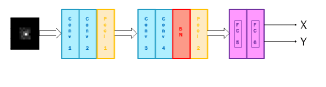
Figure 4: VGG6 model architecture.

The specific properties of the VGG6 models used here are listed in Table 1.

Table 1: VGG6 models

Layer (type)	Output shape	$\#$ of param.
V1 model - 34K parameters
conv1 (Conv2D)	(None, 14, 14, 16)	160
conv2 (Conv2D)	(None, 12, 12, 16)	2320
max-pool2d (MaxPooling2D)	(None, 6, 6, 16)	0
conv3 (Conv2D)	(None, 4, 4, 32)	4640
conv4 (Conv2D)	(None, 2, 2, 32)	9248
bn2 (BatchNormalization)	(None, 2, 2, 32)	128
max-pool2d-1 (MaxPooling2D)	(None, 1, 1, 32)	0
flatten (Flatten)	(None, 32)	0
fc-1 (Dense)	(None, 512)	16896
fc-out (Dense)	(None, 2)	1026
Total param.: 34418; trainable param.: 34354
V2 model - 214K parameters
conv1 (Conv2D)	(None, 16, 16, 32)	832
conv2 (Conv2D)	(None, 12, 12, 32)	25632
max-pool2d (MaxPooling2D)	(None, 8, 8, 32)	0
conv3 (Conv2D)	(None, 6, 6, 64)	18496
conv4 (Conv2D)	(None, 4, 4, 64)	36928
bn2 (BatchNormalization)	(None, 4, 4, 64)	256
max-pool2d-3 (MaxPooling2D)	(None, 2, 2, 64)	0
flatten-1 (Flatten)	(None, 256)	0
fc-1 (Dense)	(None, 512)	131584
fc-out (Dense)	(None, 2)	1026
Total param.: 214754; trainable param.: 214626

4 Application to Simulated Data

4.1 Simulation Code

As a precursor to exploring the effectiveness of the VGG centering on real WFPC2 images, an in-house image simulation code was written to construct star-field images that specifically emulate processed WFPC2 exposures. Given an ePSF profile – such as those used in the standard hst1pass source detection and centering software – and an input list of star positions and magnitudes, simulated image files are produced for each of the four WFPC2 chips. The simulation code includes the effects of gain, exposure time, field-dependent sensitivity and vignetting (via actual WFPC2 flatfield-correction files), A/D saturation, column bleeding, charge transfer inefficiency charge shifts (CTI), sky background, cosmic rays, and bias and dark current. Poisson noise is added for the appropriate sources of such, as well as Gaussian readout noise. Finally, the images are given bias, dark-current, and flatfield corrections yielding the equivalent of processed WFPC2 images.

Note that actual WFPC2 images exhibit a field dependent ePSF requiring interpolation within a spatial grid of ePSFs, in practice. For the trials presented here we restrict ourselves to a uniform ePSF for each chip. In effect, all of the simulated star images are as if they were found within the central portion of a real WFPC2 chip. Also, CTI and cosmic rays have been ”turned off” in the present simulations. For these simulation tests we use the hst1pass library central ePSF for filter F555W to construct constant-ePSF images of the PC and WF3 chips in this filter.

Our simulation code does not include the 34th-row systematic error or the astrometric effects of optical distortion, as we are concerned here only with the PSF modeling.

4.2 Simulation Input

To generate a WFPC2-type exposure we start with an input catalog of positions and magnitudes. We note that throughout this discussion magnitudes are instrumental (uncalibrated) magnitudes. We begin with the filter F555W test, for which the input catalog is created as follows. One of the F555W 160-sec exposures is processed with hst1pass — specifically the PC chip — to produce a list of detections with input $(x,y)$ positions and instrumental magnitudes. We include all objects with quality parameter q = 0.0 to 1.0. Note that objects with q = 0.0 are detected but not precisely centered by hst1pass as they are deemed saturated; hst1pass assigns such objects a fractional pixel-position of 0. This does not matter since we discard the fractional part of the $(x,y)$ positions of all objects in the list, and assign randomly chosen pixel fractions. This ensures there is no fractional-pixel bias in our input catalog. This input list is then used to generate a PC and a WF3 image with the simulation code described in Sec. 4.1. The magnitude distribution of this input list is the natural magnitude distribution of stars in cluster NGC 104, and as such most objects are toward fainter magnitudes. Thus, the training process will be dominated by stars with rather faint magnitudes. We will refer to this sample as “natural”.

However, we also want to better explore the performance of the DL algorithm at the bright end. Accordingly, we have created a second input catalog with an artificial magnitude distribution, such that bright stars are overly represented. We refer to this sample as “bright-enhanced”.

4.3 Simulation Results

In Table 2 we show the total number of input objects, (N_tot), that went into the DL modeling process. The training+validation sample uses $80\%$ of these objects, while the testing is done on the remaining $20\%$. The total number of testing objects, (N_test), is shown in column 3 of Tab. 2. In column 4, (N_eval), we indicate the average number of objects used to evaluate the standard deviation of differences in position between the input (true) values and the DL-determined ones. This latter number is derived from the N_test sample, but trimmed within a fixed magnitude range — to ensure we are dealing with well-measured stars — and further trimmed by eliminating $3\sigma$ position-difference outliers in an iterative procedure. The magnitude range of N_eval for the natural-magnitude distribution sample is thus limited to the subset of stars with magnitudes between 15.0 and 18.0, and for the bright-enhanced magnitude distribution sample to between 13.0 and 15.0.

Table 2: Simulated-data sample statistics

Sample	Ntot	Ntest	Neval
Natural	4648	930	$\sim 600$
Bright-enhanced	8493	1699	$\sim 530$

In Figure 5 we show the loss function of the training and testing samples as a function of model epoch. This is run for the natural-magnitude distribution sample and for a raster size of $6\times 6$ pixels; both V1 and V2 models are shown. The plots indicate that model V2 achieves a better loss trend than does model V1.

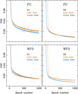
Figure 5: Simulated data for the natural-magnitude distribution sample: the loss function and its dependence on epoch for the $6\times 6$-pixel raster run. Both PC and WF3 chips for models V1 and V2 are shown. Recall that WF3 is more severely undersampled compared to the PC, by roughly a factor of 2.

Next, we plot position differences as a function of magnitude for both the natural and bright-enhanced samples in Figure 6. The realization shown is for the PC with raster size of $6\times 6$ pixels and for version V2 of the DL model (see 3.2).

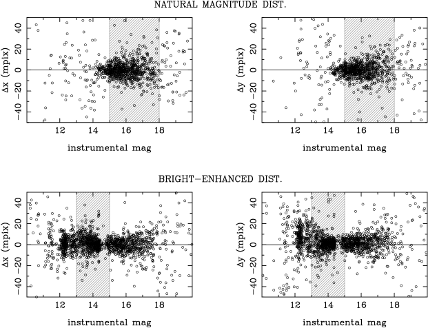
Figure 6: Position differences (DL-derived minus true) as a function of magnitude for simulated data. This realization is for the PC, using a raster size of $6\times 6$ pixels, and model V2. Both natural (top) and bright-enhanced (bottom) magnitude distribution samples are shown. The hashed areas highlight the restricted magnitude range over which standard deviations are calculated.

In the bright-enhanced sample, the larger scatter in $\Delta y$ compared to that in $\Delta x$ at magnitudes $\leq 13.5$ is due to saturation and bleeding effects along the read-out direction of the chip. Nevertheless, the bright end still has a tight position-difference distribution for the sample that includes many more bright stars in the training process. This indicates that the bright stars can be reliably DL-modeled, if special attention is given them.

In what follows, we will use the standard deviation of the position differences as a measure of the error in each model realization. We use values obtained from samples within the restricted magnitude ranges listed above, and with $3-\sigma$ outlier clipping. We explore these errors as a function of the raster size cutout around each object. Simulations for both the PC and WF3 are tested, and for both V1 and V2 DL models. Again, both the natural and bright-enhanced samples are studied.

The standard deviations of position differences are shown in Figure 7. Error bars were estimated for the $6\times 6$-raster experiment by repeating the experiment five times, i.e., the uncertainty estimates are based on the scatter produced by the randomness of the selection of the $20\%$ test sample in the DL code. For comparison, we also indicate the value of the standard deviation calculated from hst1pass-derived positions obtained on these same simulated images, within the restricted central 1/9 area of the chip. We use raw hst1pass positions, i.e., uncorrected for 34-row and optical distortion, since the simulations do not incorporate these effects. The generic hst1pass code was applied only to the natural magnitude distribution sample, as it is not optimized for bright objects.

Fig. 7 indicates that version V2 of the DL model gives better results than does V1; this is in agreement with the indication by the loss function shown in Fig. 5. Small raster-size cutouts tend to give better results than do large ones, for the natural magnitude sample. For WF3, there appears to be a minimum at a raster size of around 6 pixels, while for the PC this value is also near minimum. Therefore, in our exploration of real data, we will adopt a fixed $6\times 6$ raster size for both the PC and the WF chips.

The hst1pass standard deviations are in reasonable agreement with the low portion of the DL values, at raster sizes between 4 and 8 pixels. This is not surprising, since the simulated images were built with an ePSF that is exactly that from the hst1pass standard library. In fact, for the WF3 chip, the DL V2 results are even somewhat better than those of hst1pass. Finally, for the bright-enhanced sample, it is evident that excellent results can be obtained with the DL methodology, given adequate input training data.

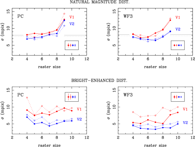
Figure 7: Standard deviation of position differences as a function of raster size for simulated PC and WF3 images. Continuous lines correspond to the $x$ coordinate, and dashed lines to the $y$ coordinate, The two versions of the DL model are shown. Also, both natural and bright-enhanced magnitude distribution samples are plotted, as labeled. For the natural sample we also indicate with horizontal solid and dashed lines the standard deviations in each coordinate obtained from hst1pass-based positions. For the bright-enhanced sample there are no such values, since hst1pass is not designed to center these stars. Typical error bars obtained for the $6\times 6$-pixel raster experiment are given in the legend box.

5 Application to Real Data

5.1 Input and DL model

For real WFPC2 images it is clear that we do not readily have “true” positions in order to train the DL technique. Is it possible to form a catalog of positions that are sufficiently precise to serve this purpose? The NGC 104 Gilliland data set offers such a possibility; with over 600 exposures taken at various small offsets (up to 2 PC pixels, see Fig. 1) an average catalog can be built and used as “true” positions for training. We construct this average catalog by first transforming the positions from each exposure into those of the first exposure thus placing all exposures on the system of the first one. The positions to be used are those from the hst1pass runs. Only objects with quality parameter q = 0.0001 to 1.0 are used; thus bright stars, with inferior hst1pass centers, do not participate in this process. The polynomial transformation between reference and target exposure includes up to 3rd order terms. Once all are on the same system, the repeated measures for the same star are combined to form a mean position, after iteratively removing any measures more than $3\sigma$ from the mean. The resulting average catalog’s positions can then be transformed back to the system of each individual exposure, providing what will serve as a “true” position to correspond to each star’s cutout raster.

To avoid having to consider effects from the variable PSF across each WFPC2 detector, only stars in the central part of each chip are used, specifically, the central third of both the $x$ and $y$ coordinate range. We further refine the input list by discarding all objects that have a neighbor within 5 pixels, such that random blends and crowdiness do not confuse the training process.

Note that the large number of exposures, and the distribution of fractional-pixel offsets among them, will serve to effectively average out any pixel-phase bias present in the hst1pass positions, as well improving the precision well beyond that of any single exposure. It is this that allows us to use the hst1pass-based positions to form a sufficiently precise and systematic-free set of “true” positions to do DL modeling.

In practice, for each exposure we extract rasters of $6\times 6$ pixels around each object in the input list. The DL model can then be trained and verified using the average catalog positions — always in the system of the corresponding exposure — along with the cutout rasters. Although confined to the central area of each chip, the 636 exposures in filter F555W provide an ample amount of input data to construct a DL model. A separate run/model is made for each of the four WFPC2 chips. The model architecture is the same as that used for the simulated data, i.e., the two versions of VGG6 described in Sec. 3.2.

In a similar manner, separate DL models can also be constructed based on the F814W data set, which has 654 exposures. The number of useful stars per exposure and chip in the input lists is between 350 and 400 objects for the F555W data set, and between 430 and 480 for the F814W data set. The total numbers of objects that enter into the model building for the entire set of over 600 exposures are listed in Table 3 for each chip and filter. These numbers are a factor of between $\sim 50$ and 70 larger than the number of input objects in the simulation experiments (see Tab. 2).

Table 3: Number of input objects per chip and filter

Filter	Nexp	NPC	NWF2	NWF3	NWF4
F555W	636	235912	231391	253207	224953
F814W	654	289430	297036	310076	282431

Figure 8 shows the resulting loss-function trends with epoch for the F555W data. Each panel represents a different chip and version of the DL model, as labeled. Figure 9 shows the equivalent information for the DL modeling of the F814W data. The second version of the model appears to perform better than the first version, especially for the PC detector.

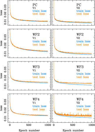
Figure 8: Real F555W data: the loss-function trend with epoch for the four chips and two versions of the DL model.

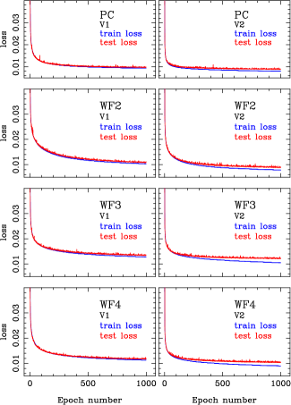
Figure 9: Real F814W data: the loss function trend with epoch for the four chips and two versions of the DL model.

5.2 Real-Data Results

The models derived in Sec. 5.1 can be applied to all (hst1pass) detections in all exposures of the real data sets upon which they were built, namely the NGC 104 Gilliland sets in F555W and F814W, provided one also adheres to the central-area limits imposed by the presumption of non-variance of the PSF. It would be interesting to see if these same models, derived from NGC 104 data, can be applied to other WFPC2 data sets that have sufficient numbers of offset exposures and stars per exposure to allow evaluation of the astometric accuracy of the resulting star centers.

To this end, a search was made of the WFPC2 archive of observations to identify any such data sets. Specifically, we require data sets of targets sufficiently rich in measurable stars and containing a number of repeated exposures with small offsets. The repeated, offset exposures will allow for the detection of any pixel-phase bias, while numerous stars are needed to ensure a reliable transformation from any given exposure into a chosen reference one, even while considering only the central 1/9th of each chip. Not surprisingly, there are very few such data sets in the archive, and these all are in dense areas of not-too-distant globular clusters. In Table 4 we summarize the properties of candidate data sets in each of the two filters. The NGC 104 data sets used to build the models are listed first, in bold letters, while the subsequent targets are listed by observation date.

Table 4: Data sets used to test the DL models

Target field	Nexp	Exp. time	Epoch
F555W
NGC 104	636	160	1999.5
NGC 6752 - PC	118	26	1994.6
NGC 6441	36	160	2007.3
NGC 6341	28	100	2008.1
F814W
NGC 104	654	160	1999.5
NGC 6752 - PC	109	50	1994.6
NGC 6656	170	260	1999.1-2000.1
NGC 6205	25	140	1999.8
NGC 5139	24	80	2008.1

The appropriate DL models, by filter and chip, were applied to each of these sets. Star detection and cutout rasters were made using hst1pass star centers as rough, preliminary positions and confining the test samples to the central area of each chip. Polynomial transformations of star positions from each exposure into those of a selected reference exposure were then made in order to evaluate the standard errors of the DL-model positions.

We present the results for our test data sets in plots similar to those in Fig. 2. However, in this case the standard errors are plotted as a function of the pixel phase of the offset from the reference exposure, instead of the full offset itself. In other words, this is the fractional part of the full offset, (shifting all offsets by a constant, if need be, to ensure they are positive). We designate this offset phase $\phi$, and its value ranges from 0 to 1.

As such, in Fig. 2, the pixel-phase bias manifests itself as either a “W” or ”V”-shaped curve for the PC and WF chips, respectively. When plotting versus pixel-phase, these curves are essentially folded and the bias shows itself as a curve with minimum standard error at $\phi$ = 0 and 1, and rising to a maximum at mid values of $\phi$. In the absence of any pixel-phase bias, the standard error curves should be flat as a function of offset phase.

For each cluster and filter — as specified in the label above each plot — we show these standard error curves for positions obtained with hst1pass, and with the VGG6 model. For NGC 104 we show results for both versions of the VGG6 model, while for the remaining clusters we show only the VGG6 version V2 results, as these were deemed the best.

The results for NGC 104 in F555W presented in Figure 10 show a vast improvement of the VGG6 positions over those obtained with hst1pass in all four chips. Also version V2 of the VGG6 model gives slightly better results than does version V1. The DL positions show almost no pixel-phase bias.

Next, we present results for the other data sets observed in filter F555W. Keep in mind the DL models applied to these sets were based on the NGC 104 data, while the target sets were generally taken at a different observation epoch. Also, none of these sets have the number of repeats or excellent offset-phase $\phi$ coverage of the NGC 104 data set, making the standard error plots noisier and less coherent. Finally, consideration of the observation exposure times and inherent richness of some target clusters leads to a range in overall quality of the standard-error plots.

The data set for NGC 6752 had only PC observations, in both filters. This is a bit unfortunate, since this data set is the only one taken at an earlier epoch compared to the NGC 104 sets (see Tab. 4). Results shown in Figure 11 indicate that the VGG6 model is an improvement for the F555W data set. However, the sampling is unfortunate as we miss the mid portion of this figure where the presence of pixel-phase bias shows itself best.

Results for NGC 6441 and NGC 6341 in filter F555W are presented in Figures 12 and 13. For the PC there is marked improvement in the VGG6 positions compared to the hst1pass ones. However, for the WF there is only marginal improvement. Both these data sets were taken at a much later epoch than the NGC 104 set. Presumably, the VGG6 PSF model based on the NGC 104 data set is likely no longer representative for the later sets, and this results in the retention of some pixel-phase bias. This is manifested more so in the WF chips since these are the most undersampled.

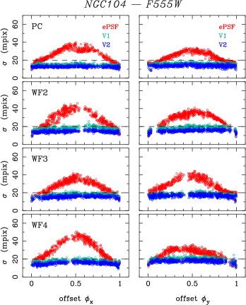
Figure 10: Standard error of the transformation (of a target exposure into the reference exposure) as a function of offset phase. x and y- coordinate values are shown in the left and right panels, respectively, and each row represents a chip, as labeled. A curve exhibiting larger standard errors near mid pixel-phase values indicates the presence of pixel-phase bias in the positions. Three centering algorithms are presented and color-coded, as labeled: classic ePSF/hst1pass and DL VGG6 versions V1 and V2. Note the flat curves at $\sim 13-15$ mpix obtained for the DL centers. These results are for exposures of NGC 104 in filter F555W.

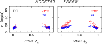
Figure 11: As in Fig. 10, only for NGC 6752 in F555W.

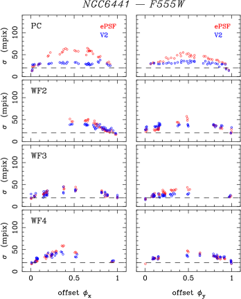
Figure 12: As in Fig. 10, only for NGC 6441 in F555W.

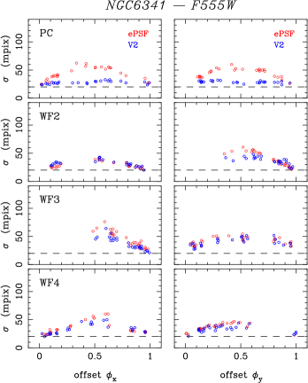
Figure 13: As in Fig. 10, only for NGC 6341 in F555W.

Turning our attention to the F814W data sets, Figure 14 shows the standard errors of the various centering algorithms as applied to the NGC 104 exposures in this filter. The results are qualitatively similar to those of the F555W data set for this cluster, i.e., both V1 and V2 showing much less pixel-phase bias compared to hst1pass. Although, for the PC, the improvement is not as dramatic in F814W as it was in F555W. This is probably explained by the F814W images being better sampled (especially in the PC) at these longer wavelengths and, thus, it would be expected that any pixel-phase bias present in the hst1pass centers would be less severe.

Next, we show the results for the PC-only F814W data set of NGC 6752 in Figure 15. Improvement in the standard errors of the DL positions over those from hst1pass is barely perceptible, at best. The limited pixel-phase coverage hinders any real conclusion here.

Also in filter F814W, we present results for three other clusters. The NGC 6656 and NGC 6205 data sets were taken at about the same epoch as that of NGC 104, (upon which the DL model is based), while the NGC 5139 set is at a much later epoch (see Tab. 4). Figures 16, 17 and 18 present results for these clusters’ data sets. For the PC, there is little to no improvement of the VGG6 positions compared to the hst1pass ones. However, for the WF chip, there is notable improvement seen in Figs. 16 and 17. Taken at about the same epoch as the NGC 104 set, it is reasonable that the PSF for these clusters’ data sets would be similar to that for the NGC 104 set. Presumably, it is because of this that the VGG6 model works reasonably well correcting the bias in these two sets.

For the later epoch NGC 5139 set (Fig. 18 ), there is only marginal improvement. This would be in keeping with the supposition that because of the large epoch difference, the VGG6-derived model is no longer appropriate. The PC results for NGC 5139 are also rather noisy and thus inconclusive. This is because only of the order of 25 stars were available for each PC solution, rather than the typical number of the order of 100 to a few hundred.

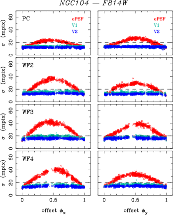
Figure 14: As in Fig. 10, only for NGC 104 in F814W.

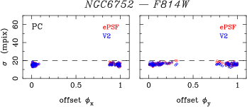
Figure 15: As in Fig. 10, only for NGC 6752 in F814W.

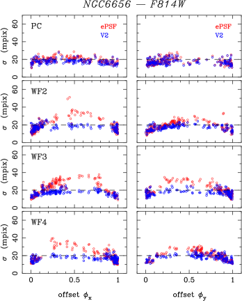
Figure 16: As in Fig. 10, only for NGC 6656 in F814W.

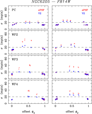
Figure 17: As in Fig. 10, only for NGC 6205 in F814W.

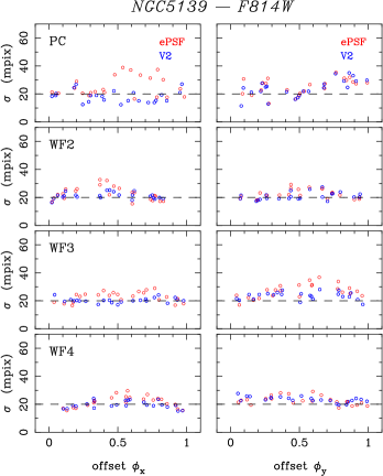
Figure 18: As in Fig. 10, only for NGC 5139 in F814W.

5.3 Per-star Comparison Examples

Figures 10 through 18 represent one way of illustrating the precision of DL centering compared to that of ePSF/hst1pass, one in which pixel phase error is highlighted. Another means of comparison can be made that more directly mimics how stellar centers are employed in practice, e.g., in proper-motion studies. How do the standard errors per exposure shown in the aforementioned figures translate into positional precision for individual stars when averaged over multiple exposures at a given epoch? To answer this question we select three exemplary data sets and apply the following procedure.

Star positions for each exposure are transformed into the system of a chosen reference exposure (just as in Figures 10 through 18). Once on a common system, repeat measures of each star are averaged, discarding any egregious outliers via a conservative sigma clipping. The resulting rms about each star’s mean position is an indicator of its astrometric precision. Distributions of the rms values for the ensemble of stars can then be used to directly compare the different centering methods. Figure 19 shows such rms distributions for three data sets: NGC 104 in F555W, both PC and WF3; and NGC 6341 in F555W, the PC. The distributions, as shown, are constructed by summing unit-area Gaussian functions of an adequately narrow width (1.3 mpix) at the location of each star’s rms value along x or y.

As can be seen in the figure, the VGG6-V2 centers outperform those of ePSF/hst1pass. Averaged over the stars depicted in Fig. 19, the ratio of rms values from the two methods ranges from 1.4 to 1.8 for these three examples, i.e., the ePSF/hst1pass errors are from 40 to $80\%$ larger. Admittedly, the three specific cases selected here are among those in which the corresponding standard-error plots already show the DL centers to be superior. It should be noted that the VGG6-V2 model was trained on a subset of the images in the NGC 104 exposures, while the NGC 6341 data set is completely independent. Nevertheless, in these selected cases the improvement is substantial, as can be judged directly by the scatter about the average stellar positions.

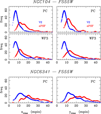
Figure 19: Distributions of rms about mean stellar positions as derived from repeated measures, based on hst1pass/ePSF centers (red symbols) and VGG6-V2 centers (blue symbols). Distributions along both x and y axes are shown for NGC 104 (PC and WF3) and for NGC 6341 (PC), all in F555W. The distributions from hst1pass are broader and shifted to higher values compared to those of VGG-V2. These can be compared to the range in standard deviation seen in the corresponding solutions of these same observations, Figs 10 and 13.

5.4 Two Ancillary Tests

We have performed two more tests involving the DL centering procedure and think it worthwhile including a description of these here.

First, we explore the possibility of taking our DL models based on simulated exposures and applying them to real WFPC2 data. The utility of such an approach would be considerable, given the dearth of available WFPC2 data sets (such as those of NGC 104) that have the required star density and repeated offset exposures to allow for the construction of an empirical DL model. The ability to build reliable DL models from simulated images would provide a means of reducing WFPC2 exposures at any epoch, yielding star centers free of pixel-phas bias. As a naive test, we have applied to the real (F555W) exposures of NGC 104 the DL model of Sec. 4.3, which was based on our simulations of the F555W NGC 104 data set. In effect, this is a test of just how well the simulated images mimic real ones. Alas, the resulting standard-error plots showed the same “W” and “V”-type curves (as in Fig. 2 for instance) indicating significant pixel-phase bias. Recall that the simulation code relies on the hst1pass library ePSF profiles, which our other tests have shown are not ideally suited for the NGC 104 data sets. An alternate means for constructing a faithful WFPC2 ePSF is required.

Second is a test that is of a completely different nature. We experiment to see whether any improvement is to be gained by modifying the real-data DL modeling procedure of Sec. 5.1 with a “second iteration” of the average catalog used as the “ ground truth”. In the original implementation, the catalog was constructed from the trimmed mean of hst1pass positions for well-measured stars over all 636 exposures. Perhaps a superior average catalog could be built from positions derived by applying the “first-iteration” DL model to all 636 NGC 104 exposures and using these to form a trimmed mean for each star, thus greatly reducing any remnant of the original hst1pass positions. The second-iteration DL model could then be applied to all 636 exposures and evaluated as before, by plotting standard error versus offset phase such as in Fig 10. Having done so, we find no significant improvement over the results of the first-iteration DL model.

We thus conclude that critical to improving DL-derived positions is the quality of the initial input “truth” that goes into the model building. Thus far we find ourselves limited to the data sets of NGC 104; perhaps a more sophisticated scheme for combining data sets of different targets but of similar ePSF composition can be developed. This will have to be the subject of future study.

6 Summary

Pixel-phase bias, acknowledged early in the studies of WFPC2 images (Anderson & King, 2000), remains a frustrating source of systematic error even when the ePSF fitting method and library specifically constructed to address the undersampling issues of WFPC2 are used to center star images.

This bias can be difficult to pinpoint, and only specially-designed data sets are appropriate to diagnose and characterize it. It’s amplitude can be as large as 50 mpix (i.e., 2.3 mas for the PC, and 5 mas for the WF) even when using state-of-the-art, traditional centering algorithms. Such pixel-phase bias is propagated into positions as unaccounted-for noise, as subsequent astrometric corrections (such as the 34th-row and optical distortion corrections) combined with large offsets between repeated images will smear out this systematic error and make it appear a random one.

We re-address the elimination of pixel-phase bias by using a novel approach based on a DL scheme, where the PSF is learned via training of a VGG6 network with simulated images, as well as with real images.

Simulated WFPC2 images helped us develop, test and characterize the DL model. We obtain errors of the order of 7-8 mpix for the PC and 6-7 mpix for the WF for typical simulated-star profiles. High signal-to-noise, very well-measured stars can achieve 5-mpix errors in the PC and 3 mpix in the WF.

Subsequently, we use real WFPC2 images to build another set of DL models. The unique NGC 104 data set of over 600 exposures, taken with a range of fractional-pixel offsets, is used to construct an average catalog of positions that is precise and bias free. We adopt this catalog as the “truth” in the training process for the real images. These DL models, one for each WFPC2 detector, are then applied to all detected stars to derive DL-based positions. These are then compared internally, within the repeated exposures, to test for pixel-phase bias and astrometric precision, as detailed in Sec. 5.2. The DL models derived from the real NGC 104 data set are applied not only to the NGC 104 data, but also to suitable data sets of other cluster fields. For now, we have limited all our analysis to the central portion of each WFPc2 chip, in order to avoid complications due to a field-varying PSF. Note that this entire procedure is performed, separately, on real images in two filters: F555W and F814W.

Doing so, we obtain excellent results for the NGC 104 data sets. Positional errors are determined from the standard errors in Figs. 10 and 14, after appropriate division by $\sqrt{2}$ since these standard errors include the measurement error of the star on the reference image and that on the test image. The best error values are achieved using version V2 of the VGG6 model. For the PC we obtain errors of the order of 9 to 10 mpix in filter F555W, and 8.5 mpix in F814W. For the WF chips we obtain 10 to 11 mpix in F555W, and 8.5 to 9.5 mpix in F814W.

The DL models built on the NGC 104 data sets are also applied to other cluster data sets, as mentioned above. In these cases we generally obtain significantly improved results over those of the classic ePSF centering procedure. Exceptions are those clusters whose observing epoch differed by many years from that of NGC 104, the set used to build the DL models. Presumably, the PSF changes with time to an extent that renders the DL models less of a good fit. Nonetheless, in every case the DL positions performed at least as well as the classic ePSF ones.

7 Future Work

These initial results obtained with a relatively simple form for the DL model are very encouraging. Still, there are some obvious refinements that could be made to improve the procedure, and these we hope to explore in subsequent studies. An immediate objective is to build a model where the PSF is allowed to vary with position on the chip. It is known that the variation of the PSF across each chip is rather mild, (Anderson & King, 2000), therefore this variation should be easily captured by a straightforward adjustment of the DL model. Note that the slight increase in model complexity will be more than compensated for by the increase in the number of stars per chip available to train the model, a factor of 9 more stars than in our present tests, once the entire chip is modeled.

Next, we plan to automatically search the hyperparameters of the DL model to further refine the training process. More imporantly, we plan to explore other alternatives such as Residual Networks architectures (He et al., 2016) with skip-connections, which allow building deeper neural networks, or Symbolic Regression (Schmidt & Lipson, 2009) to infere analytical expressions from the observed data.

Finally, we will strive to incorporate more WFPC2 data sets into future model building, as well improve the of the simulated images.

References

- Anderson (2022) Anderson, J. 2022, One-Pass HST Photometry with hst1pass, Instrument Science Report ACS 2022-02, ,
- Anderson & King (1999) Anderson, J., & King, I. R. 1999, PASP, 111, 1095
- Anderson & King (2000) —. 2000, PASP, 112, 1360
- Baena-Gallé et al. (2022) Baena-Gallé, R., Girard, T. M., Casetti-Dinescu, D. I., & Martone, M. 2022, in press:Proceedings of the XV Scientific Meeting of the Spanish Astronomical Society 2022
- Casetti-Dinescu et al. (2021) Casetti-Dinescu, D. I., Girard, T. M., Kozhurina-Platais, V., et al. 2021, PASP, 133, 064505
- Castro-Ginard et al. (2022) Castro-Ginard, A., Jordi, C., Luri, X., et al. 2022, A&A, 661, A118
- Chollet & others (2018) Chollet, F., & others. 2018, Keras: The Python Deep Learning library, Astrophysics Source Code Library, record ascl:1806.022, ,
- Dropulic et al. (2021) Dropulic, A., Ostdiek, B., Chang, L. J., et al. 2021, ApJ, 915, L14
- He et al. (2016) He, K., Zhang, X., Ren, S., & Sun, J. 2016, in 2016 IEEE Conference on Computer Vision and Pattern Recognition (CVPR), 770–778
- Henghes et al. (2022) Henghes, B., Thiyagalingam, J., Pettitt, C., Hey, T., & Lahav, O. 2022, MNRAS, 512, 1696
- Herbel et al. (2018) Herbel, J., Kacprzak, T., Amara, A., Refregier, A., & Lucchi, A. 2018, J. Cosmology Astropart. Phys, 2018, 054
- Kim & Brunner (2017) Kim, E. J., & Brunner, R. J. 2017, MNRAS, 464, 4463
- Lecun et al. (2015) Lecun, Y., Bengio, Y., & Hinton, G. 2015, Nature, 521, 436
- Martínez-Palomera et al. (2022) Martínez-Palomera, J., Bloom, J. S., & Abrahams, E. S. 2022, AJ, 164, 263
- Schmidt & Lipson (2009) Schmidt, M. D., & Lipson, H. 2009, Science, 324, 81
- Simonyan & Zisserman (2014) Simonyan, K., & Zisserman, A. 2014, arXiv e-prints, arXiv:1409.1556