Distributionally robust model predictive control for wind farms

Abstract

In this paper, we develop a distributionally robust model predictive control framework for the control of wind farms with the goal of power tracking and mechanical stress reduction of the individual wind turbines. We introduce an ARMA model to predict the turbulent wind speed, where we merely assume that the residuals are sub-Gaussian noise with statistics contained in an moment-based ambiguity set. We employ a recently developed distributionally model predictive control scheme to ensure constraint satisfaction and recursive feasibility of the control algorithm. The effectiveness of the approach is demonstrated on a practical example of five wind turbines in a row.

1 Introduction

A large part of green energy production is currently covered by wind farms (WF), where several wind turbines (WT) are placed in close proximity to each other to reduce the cost of cabling and maintenance. One problem that occurs in such an environment is that each wind turbine generates a wake that moves downstream and is characterized by a flow velocity deficit and increased turbulence intensity Barthelmie et al. (2007). The flow velocity deficit directly impacts the power production of downstream turbines Barthelmie et al. (2010), while the increased turbulence intensity increases the fatigue loads Bossuyt et al. (2017).

In this paper, a distributionally robust model predictive controller (DR-MPC) is developed as a supervisory controller for a wind farm with the primary objective of dynamically allocating a required wind farm power reference to the individual wind turbines in the field. The WT power references are then tracked by underlying local WT controllers, which operate on a much faster timescale (millisecond range) compared to the WF controller (second range). A secondary objective of the wind farm controller is to reduce fatigue loads of the turbines to increase their overall lifetime. The DR-MPC algorithm is based on our previous publication Mark and Liu (2023), but has been extended to include cost functions for output variables.

Related work: In Riverso et al. (2016), the authors consider the same setup as we do and use a stochastic MPC (SMPC) to design a supervisory control system for wind farms, adopting the probabilistic SMPC framework from Farina et al. (2013). However, their approach is based on the assumption that the true wind speed is normally distributed and the moments are known exactly. In Boersma et al. (2019), a scenario-based SMPC for power reference tracking is developed, where Gaussianity of the wind speed distribution is assumed. Fatigue load reduction is not considered explicitly in this work. The authors of Spudić et al. (2011) investigated a deterministic MPC approach for wind farm control. Similar to our approach, the goal was to track power and reduce mechanical stress, however, the stochasticity of the wind is neglected and assumed to be constant over the prediction horizon. This approach was extended to a distributed MPC in Spudić et al. (2015). In terms of wind turbine control, several papers have been published that address fatigue reduction, such as Evans et al. (2014), where a robust MPC was developed for oscillation damping, or Gros and Schild (2017), where an economic nonlinear MPC was applied to reduce structural and actuator fatigue.

1.1 Notation

A probability space is defined by the triplet $(\Omega,\mathcal{F},\mathbb{P})$, where $\Omega$ is the sample space, $\mathcal{F}$ the Borel $\sigma$-algebra on $\Omega$ and $\mathbb{P}$ the probability measure on $(\Omega,\mathcal{F})$. The set of all probability distributions supported on $\Omega$ with finite second moment is $\mathcal{M}(\Omega)$. Given an event $E_{1}$ we define the probability occurrence as $\mathbb{P}(E_{1})$ and the conditional probability given $E_{2}$ as $\mathbb{P}(E_{1}|E_{2})$. For a random variable $w$, we define the expected value as $\mathbb{E}(w)$, whereas the conditional expectation of $w$ conditional to a random variable $x$ is denoted as $\mathbb{E}(w|x)$. The weighted 2-norm w.r.t. a positive definite matrix $Q=Q^{\top}$ is $\|x\|_{Q}^{2}=x^{\top}Qx$. Positive definite and semidefinite matrices are indicated as $A\succ 0$ and $A\succeq 0$, respectively. The pseudo inverse of a matrix $A$ is denoted as $A^{\dagger}$. The stacked column vector $x\in\mathbb{R}^{Nn}$ of subvectors $x_{1},\ldots,x_{N}\in\mathbb{R}^{n}$ is defined as $x=\mathrm{col}_{i=1,\ldots,N}(x_{i})$. The Kroneker product is denoted as $\otimes$.

1.2 Outline

In Section 2, we introduce the wind farm model and pose the general optimization problem of interest. Section 3 is devoted to the theoretical background of the distributionally robust MPC, which is based on our previous publication Mark and Liu (2023). In Section 4, we perform two simulations using a wind farm with five wind turbines in a row. The paper closes with Section 5, where we summarize the results and provide a brief outlook.

2 Problem description

In this paper, we use a linearized version of the NREL WT as proposed by Riverso et al. (2016), where the $i$-th WT is described by a linear time-invariant system of the form

$$x_{i}(k+1) =A_{i}x_{i}(k)+B_{i}u_{i}(k)+E_{i}w_{i}(k)$$ (1a)

$$y_{i}(k) =C_{i}x_{i}(k)+D_{i}u_{i}(k)+F_{i}w_{i}(k)$$ (1b)

with state $x_{i}=(\beta_{i},\omega_{i,\mathrm{r}},\omega^{\mathrm{f}}_{i,\mathrm{g}})-(\beta_{i,0},\omega_{i,\mathrm{r0}},\omega_{i,\mathrm{g0}})$, input $u_{i}=P^{\mathrm{wt}}_{i,\mathrm{ref}}-P^{\mathrm{wt}}_{i,0}$, disturbance $w_{i}=\tilde{w}_{i}-w_{i,0}$ and output $y_{i}=(F_{i,\mathrm{t}},T_{i,\mathrm{s}})-(F_{i,\mathrm{t0}},T_{i,\mathrm{s0}})$. The individual components are the blade pitch angle $\beta_{i}\>[\mathrm{{}^{\circ}}]$, the rotor angular velocity $\omega_{i,\mathrm{r}}\>[\mathrm{rad/s}]$, the filtered generator angular velocity $\omega_{i,\mathrm{g}}\>[\mathrm{rad/s}]$, the power reference $P^{\mathrm{wt}}_{i,\mathrm{ref}}\>[\mathrm{W}]$, the effective wind velocity $\tilde{w}_{i}\>[\mathrm{m/s}]$, the tower bending force $F_{i,\mathrm{t}}\>[\mathrm{N}]$ and the main shaft torque $T_{i,\mathrm{s}}\>[\mathrm{Nm}]$. Quantities with a subindex $0$ denote the nominal operating (linearization) point. The wind farm model is obtained by stacking $N_{\mathrm{wt}}\in\mathbb{N}$ individual WT models (1), so that $x=\mathrm{col}_{i=1,\ldots,N_{\mathrm{wt}}}(x_{i})$, $u=\mathrm{col}_{i=1,\ldots,N_{\mathrm{wt}}}(u_{i})$, $w=\mathrm{col}_{i=1,\ldots,N_{\mathrm{wt}}}(w_{i})$ and $y=\mathrm{col}_{i=1,\ldots,N_{\mathrm{wt}}}(y_{i})$, while the dynamic matrices $A-F$ are given by block diagonal stacking of the local matrices $A_{i}-F_{i}$ for all $i=1,\ldots,N_{\mathrm{wt}}$, resulting in

$$x(k+1) =Ax(k)+Bu(k)+Ew(k)$$ (2a)

$$y(k) =Cx(k)+Du(k)+Fw(k).$$ (2b)

The main objective of a wind farm controller in the above rated region is to distribute the wind power reference provided by the system operator to each wind turbine in the field while minimizing fatigue load Knudsen et al. (2015); Andersson et al. (2021). Fatigue loads result from repetitive stress reversals on a specific part of the structure, where typical fatigue prone components are the turbine tower and the generator shaft Spudić (2012). Therefore, we formulate the following infinite horizon stochastic optimal control problem

$$\!\min_{u(k)\forall k\in\mathbb{N}} \quad\mathbb{E}_{\mu^{*}}\left(\sum_{k=0}^{\infty}\|y(k)\|_{Q_{\mathrm{y}}}^{2}+\|u(k)\|_{R}^{2}\bigg{|}x(0)\right)$$ (3a)

$$\mathrm{s.t.}\hskip 9.10004pt \quad x(k+1)=Ax(k)+Bu(k)+Ew(k)$$

$$\quad y(k)=Cx(k)+Du(k)+Fw(k)$$ (3b)

$$\quad\mathbb{P}(l_{j}^{\top}u(k)\leq 1\>|\>x(0))\geq p^{u}_{j}\quad j\in\{1,\ldots,s\}$$ (3c)

$$\quad\mathbbm{1}^{\top}u(k)=0,$$ (3d)

where (3a) is an expected value quadratic cost function that penalizes deviations of the output and input with weights $Q_{\mathrm{y}}\succeq 0$ and $R\succ 0$, (3c) denotes a set of individual input chance constraints of probability level $p_{j}^{\mathrm{u}}\in(0,1)$ and (3d) enforces that the power deviations in sum are equal to zero to cover the nominal demand.

The optimization problem (3) contains several sources of intractability, i.e., (i) the control input $u$ in the presence of an additive uncertainty renders the problem infinite dimensional; (ii) the expectation in (3a) is taken w.r.t. the unknown probability distribution $\mu^{*}$ and (iii) the chance constraints (3c) are evaluated under the unknown probability measure $\mathbb{P}$. Point (i) will be tackled in Section 3.3, where we introduce a simplified affine disturbance feedback (SADF) parameterization, while the uncertainty sources (ii) and (iii) are addressed with a distributionally robust cost function and distributionally robust constraints in Sections 3.4 and 3.5 based on a moment-based ambiguity set introduced in Section 3.2.

3 Distributionally robust MPC

In this section, we use a DR-MPC scheme recently proposed by the authors Mark and Liu (2023) to approximate the infinite horizon problem (3) over a finite prediction horizon.

3.1 Prediction dynamics

To distinguish between closed-loop and predicted states and inputs, we introduce the $N$-step ahead prediction of (2a) over a horizon of length $N\in\mathbb{N}$

$$\bar{x}_{k}=\bar{A}x_{0|k}+\bar{B}\bar{u}_{k}+\bar{E}\bar{w}_{k},$$ (4)

where $\bar{x}_{k}=[x^{\top}_{0|k},x^{\top}_{1|k},\ldots,x^{\top}_{N|k}]^{\top}$ denotes the state sequence, $\bar{u}_{k}=[u^{\top}_{0|k},\ldots,u^{\top}_{N-1|k}]^{\top}$ the input sequence and $\bar{w}_{k}=[w^{\top}_{0|k},\ldots,w^{\top}_{N-1|k}]^{\top}$ the disturbance sequence, while the matrices are defined as

$$\bar{A}=\begin{bmatrix}I\\ A\\ \vdots\\ A^{N}\end{bmatrix},\bar{B}=\begin{bmatrix}0&0&\dots&0\\ B&0&\dots&0\\ AB&B&\dots&0\\ \vdots&\ddots&\ddots&0\\ A^{N-1}B&\dots&AB&B\end{bmatrix},\bar{E}=\begin{bmatrix}0&0&\dots&0\\ E&0&\dots&0\\ AE&E&\dots&0\\ \vdots&\ddots&\ddots&0\\ A^{N-1}E&\dots&AE&E\end{bmatrix}.$$

Similar to the state sequence (4), we represent the output equation (2b) in a compact form as

$$\bar{y}_{k}=\bar{C}\bar{x}_{k}+\bar{D}\bar{u}_{k}+\bar{F}\bar{w}_{k},$$ (5)

where $\bar{y}_{k}=[y_{0|k}^{\top},\ldots,y_{N|k}^{\top}]^{\top}$ and the matrices are given by

$$\bar{C}=\begin{bmatrix}C&0&\dots&0&0\\ 0&C&\dots&0&0\\ \vdots&\vdots&\ddots&\vdots&\vdots\\ 0&0&\dots&C&0\\ 0&0&\dots&0&C\end{bmatrix},\bar{D}=\begin{bmatrix}0&0&\dots&0\\ D&0&\dots&0\\ 0&D&\dots&0\\ \vdots&\vdots&\ddots&\vdots\\ 0&0&\dots&D\end{bmatrix},\bar{F}=\begin{bmatrix}0&0&\dots&0\\ F&0&\dots&0\\ 0&F&\dots&0\\ \vdots&\vdots&\ddots&\vdots\\ 0&0&\dots&F\end{bmatrix}.$$

Note that $\bar{w}_{k}$ represents a turbulent wind speed prediction that is typically non-i.i.d. and correlated in time. Therefore, to restore the sub-Gaussianity of the random variables as required by Mark and Liu (2023), we identify an auto-regressive moving average model that serves as a whitening filter for the turbulent wind speed.

3.2 ARMA model and ambiguity set

An ARMA model represents a stochastic process in terms of two polynomials, where the first one represents the auto-regressive (AR) part and the second one the moving average (MA) part Box et al. (2015). In particular, an $\mathrm{ARMA}(p,q)$ model with $p$ AR terms and $q$ MA terms is given by

$${w}(k)=\sum_{l=1}^{p}a_{l}{w}(k-l)+\sum_{l=1}^{q}b_{l}\epsilon(k-l)+\epsilon(k),$$

where $\epsilon$ is a zero-mean i.i.d white noise. In related work, e.g. Ono et al. (2013); Riverso et al. (2016), the authors make a more stringent assumption that the noise $\epsilon$ is normally distributed, which in case of wind turbulence data is prone to be wrong, cf. Van Parys et al. (2015). Therefore, we treat $\epsilon$ as a zero-mean white noise with unknown (but finite) variance $\Sigma_{\epsilon}\succ 0$. In practice, one needs to identify the ARMA model with limited data. Therefore, the empirical variance is typically falsified due to sample inaccuracies, for which we introduce a moment-based ambiguity set that captures the true variance with high probability

$$\mathcal{P}(w_{\mathrm{0}},T_{\mathrm{I}})\coloneqq\left\{\mu\in\mathcal{M}(\mathbb{R}^{n})\ \middle|\begin{array}[]{l}\mathbb{E}_{\mu}(\epsilon)=0\\ \mathbb{E}_{\mu}(\epsilon\epsilon^{\top})\preceq\kappa^{(w_{\mathrm{0}},T_{\mathrm{I}})}_{\beta}\hat{\Sigma}_{\epsilon}^{(w_{\mathrm{0}},T_{\mathrm{I}})}\end{array}\right\}.$$ (8)

Note that we parameterize the ambiguity set with the mean wind speed and turbulence intensity pair $(w_{\mathrm{0}},T_{\mathrm{I}})$. The ambiguity radius $\kappa^{(w_{\mathrm{0}},T_{\mathrm{I}})}_{\beta}$ can readily be found with (Mark and Liu, 2023, Prop. 1).

We identify for each wind turbine $i=1,\ldots,N_{\mathrm{wt}}$ an $\mathrm{ARMA}(p,p-1)$ model, which can be converted to a canonical form similar to Ono et al. (2013), i.e,

$$\psi_{i}(k+1) =A_{\psi,i}\psi_{i}(k)+B_{\psi,i}\epsilon_{i}(k)$$

$${w}_{i}(k) =C_{\psi,i}\psi_{i}(k),$$

where the matrices are defined as follows

$$A_{\psi,i}\coloneqq\begin{bmatrix}a_{i,1}&1&0&\dots&0\\ a_{i,2}&0&1&&0\\ \vdots&\vdots&&\ddots&\\ a_{i,p-1}&0&0&&1\\ a_{i,p}&0&0&\dots&0\end{bmatrix},B_{\psi,i}\coloneqq\begin{bmatrix}1\\ b_{i,1}\\ \vdots\\ b_{i,p-2}\\ b_{i,p-1}\end{bmatrix},$$

$C_{\psi,i}\coloneqq\begin{bmatrix}1&0&\cdots&0\end{bmatrix}$ and the auxiliary state vector $\psi_{i}$ is given by $\psi_{i}(k)=\begin{bmatrix}w^{\top}_{i}(k),\psi^{\top}_{i,2}(k),\dots,\psi^{\top}_{i,p}(k)\end{bmatrix}^{\top}$ with

$$\psi_{i,j}(k) =\sum_{l=j}^{p}a_{i,l}{w}_{i}(k+j-l-1)$$

$$+\sum_{l=j-1}^{p-1}b_{i,l}\epsilon_{i}(k+j-l-1)\quad\forall i\in\{1,\ldots,N_{\mathrm{wt}}\}.$$

To obtain farm-wide wind predictions, we stack the local matrices and vectors, such that $A_{\psi}=\mathrm{diag}(A_{\psi,1},\ldots,A_{\psi,N_{\mathrm{wt}}})$, $B_{\psi}=\mathrm{diag}(B_{\psi,1},\ldots,B_{\psi,N_{\mathrm{wt}}})$, $C_{\psi}=\mathrm{diag}(C_{\psi,1},\ldots,C_{\psi,N_{\mathrm{wt}}})$ and $\psi=\text{col}_{i=1}^{N_{\mathrm{wt}}}(\psi_{i})$. A $N$-step prediction of the turbulent wind speed is readily given by

$$\bar{w}_{k}\coloneqq\bar{C}_{\psi}\bar{A}_{\psi}\psi(k)+\bar{C}_{\psi}\bar{B}_{\psi}\bar{\epsilon}_{k},$$ (9)

where $\bar{C}_{\psi}\coloneqq\mathrm{diag}(C_{\psi},\ldots,C_{\psi})$,

$$\bar{A}_{\psi}\coloneqq\begin{bmatrix}I\\ A_{\psi}\\ A_{\psi}^{2}\\ \vdots\\ A_{\psi}^{N-1}\end{bmatrix},\bar{B}_{\psi}\coloneqq\begin{bmatrix}0&0&\dots&0\\ B_{\psi}&0&\dots&0\\ A_{\psi}B_{\psi}&B_{\psi}&\dots&0\\ \vdots&\ddots&\ddots&0\\ A_{\psi}^{N-2}B_{\psi}&\dots&A_{\psi}B_{\psi}&B_{\psi}\end{bmatrix},$$

while the random vector $\bar{\epsilon}_{k}$ is zero-mean and each element is i.i.d. with variance $\Sigma_{\epsilon}^{(w_{\mathrm{0}},T_{\mathrm{I}})}$.

3.3 Simplified affine disturbance feedback

To render the resulting MPC optimization problem finite dimensional, we parameterize the control input with a SADF policy, cf. Zhang and Ohtsuka (2020), of the form

$$\bar{u}_{k}=\bar{v}_{k}+\bar{M}_{k}\bar{\epsilon}_{k},$$ (10)

where the matrices are defined as

$$\bar{M}_{k}\coloneqq\begin{bmatrix}0&0&\dots&0\\ M_{1|k}&0&\dots&0\\ \vdots&\ddots&\ddots&0\\ M_{N-1|k}&\dots&M_{1|k}&0\end{bmatrix},\>\bar{v}_{k}\coloneqq\begin{bmatrix}v_{0|k}\\ v_{1|k}\\ \vdots\\ v_{N-1|k}\end{bmatrix}.$$

Next, we substitute the state prediction (4), the ARMA prediction (9) and the SADF policy (10) into the output prediction (5), resulting in

$$\bar{y}_{k} =\bar{C}\bar{x}_{k}+\bar{D}\bar{u}_{k}+\bar{F}\bar{w}_{k}$$

$${=}\underbrace{\bar{C}\bar{A}x_{0|k}+(\bar{C}\bar{B}+\bar{D})\bar{v}_{k}+(\bar{C}\bar{E}+\bar{F})\bar{C}_{\psi}\bar{A}_{\psi}\psi(k)}_{\tilde{\bar{y}}_{k}}$$

$$\quad+\underbrace{[\bar{C}\bar{B}\bar{M}_{k}+\bar{D}\bar{M}_{k}+(\bar{C}\bar{E}+\bar{F})\bar{C}_{\psi}\bar{B}_{\psi}]}_{\Psi_{k}}\bar{\epsilon}_{k}.$$ (11)

The output prediction now depends only on the initial conditions $x_{0|k},\psi(k)$, as well as on the optimization variables $\bar{v}_{k}$ and $\bar{M}_{k}$.

Remark 1

The decision variables using the SADF policy grow linearly in the prediction horizon $N$, whereas the original affine disturbance feedback policy grows quadratically Zhang and Ohtsuka (2020). Thus, the SADF policy results in less demanding optimization problems.

3.4 Cost function

We approximate the infinite horizon cost function (3a) over the prediction horizon $N$, while we replace the expected value over $\mu^{*}$ with the supremum over all distributions contained in the ambiguity set (8), i.e.,

$$J_{k} =\sup_{\mu\in\mathcal{P}}\>\mathbb{E}_{\mu}\left(\bar{y}_{k}^{\top}\bar{Q}_{\mathrm{y}}\bar{y}_{k}+\bar{u}_{k}^{\top}\bar{R}\bar{u}_{k}\bigg{|}x(k)\right)$$

$${=}\text{tr}\left(\hat{\Sigma}_{N}^{(w_{\mathrm{0}},T_{\mathrm{I}})}\big{[}\bar{H}_{\mathrm{y},k}^{\top}\bar{Q}_{\mathrm{y}}\bar{H}_{\mathrm{y},k}+\bar{H}_{\mathrm{u},k}^{\top}\bar{R}\bar{H}_{\mathrm{u},k}\big{]}\right),$$ (12)

where $\bar{H}_{\mathrm{y},k}=\begin{bmatrix}\Psi_{k}^{\top}&\tilde{\bar{y}}_{k}^{\top}\end{bmatrix}^{\top}$, $\bar{H}_{\mathrm{u},k}=\begin{bmatrix}\bar{M}_{k}^{\top}&\bar{v}_{k}^{\top}\end{bmatrix}^{\top}$, $\bar{Q}_{\mathrm{y}}=\mathrm{diag}(Q_{\mathrm{y}},\ldots,Q_{\mathrm{y}})$ and $\bar{R}=\mathrm{diag}(R,\ldots,R)$. The worst-case covariance matrix $\hat{\Sigma}_{N}^{(w_{\mathrm{0}},T_{\mathrm{I}})}$ is defined through the moment-based ambiguity set (8)

$$\hat{\Sigma}_{N}^{(w_{\mathrm{0}},T_{\mathrm{I}})} \coloneqq\sup_{\mu\in\mathcal{P}}\bigg{(}\begin{bmatrix}\bar{\epsilon}_{k}\\ 1\end{bmatrix}\begin{bmatrix}\bar{\epsilon}_{k}\\ 1\end{bmatrix}^{\top}\bigg{|}x(k)\bigg{)}$$

$${=}\mathrm{diag}\left(I_{N}\otimes\sup_{\mu\in\mathcal{P}(w_{\mathrm{0}},T_{\mathrm{I}})}\bigg{(}\begin{bmatrix}\epsilon\\ 1\end{bmatrix}\begin{bmatrix}\epsilon\\ 1\end{bmatrix}^{\top}\bigg{|}x(k)\bigg{)},1\right)$$

$${=}\mathrm{diag}(I_{N}\otimes\kappa^{(w_{\mathrm{0}},T_{\mathrm{I}})}_{\beta}\hat{\Sigma}_{\epsilon}^{(w_{\mathrm{0}},T_{\mathrm{I}})},1),$$

where the first equality follows from the i.i.d. sequence $\bar{\epsilon}_{k}$, i.e., $\bar{\epsilon}_{k}$ contains $N$-times the i.i.d. random variable $\epsilon$. For details on the reformulation steps, please refer to our recent paper Mark and Liu (2023).

3.5 Chance constraints

Since the probability measure $\mathbb{P}$ required for the chance constraints (3c) is unknown, we instead impose distributionally robust chance constraints, i.e., we enforce the chance constraint for all distributions contained in the ambiguity set (8), resulting in

$$\inf_{\mu\in\mathcal{P}}\>\mathbb{P}(l_{t,j}^{\top}\bar{u}_{k}\leq 1\>|\>x(k))\geq p^{u}_{s}$$

$$\overset{\eqref{eq:power_system:disturbance_feedback}}{=}\inf_{\mu\in\mathcal{P}}\>\mathbb{P}\bigg{(}\begin{bmatrix}\bar{\epsilon}_{k}^{\top}&1\end{bmatrix}\begin{bmatrix}l^{\top}_{t,j}\bar{M}_{k}\\ l^{\top}_{t,j}\bar{v}_{k}\end{bmatrix}\leq 1\bigg{|}x(k)\bigg{)}\geq p_{j}^{\mathrm{u}},$$

which can equivalently be expressed as second-order cone constraint via (Calafiore and Ghaoui, 2006, Thm 3.1)

$$l^{\top}_{t,j}\bar{v}_{k}\leq 1-\sqrt{\frac{p_{u}}{1-p_{u}}}\|l_{t,j}^{\top}\bar{M}_{k}(\hat{\Sigma}_{N}^{(w_{\mathrm{0}},T_{\mathrm{I}})})^{\frac{1}{2}}\|_{2}.$$ (13)

The vector $l_{t,j}$ is a lifted version $l_{j}$ from constraint (3c) to fit the dimension of the nominal input vector $\bar{v}_{k}$.

3.6 MPC optimization problem

At each time step $k\in\mathbb{N}$, we solve the following MPC optimization problem

$$\!\min_{\bar{v}_{k},\bar{M}_{k},\lambda_{k}} \text{tr}\left(\hat{\Sigma}_{N}^{(w_{\mathrm{0}},T_{\mathrm{I}})}\big{[}\bar{H}_{\mathrm{y},k}^{\top}\bar{Q}_{\mathrm{y}}\bar{H}_{\mathrm{y},k}+\bar{H}_{\mathrm{u},k}^{\top}\bar{R}\bar{H}_{\mathrm{u},k}\big{]}\right)$$ (14a)

$$\quad\mathrm{s.t.} \bar{y}_{k}=\tilde{\bar{y}}_{k}+\Psi_{k}\bar{\epsilon}_{k}$$ (14b)

$$\bar{z}_{k}=\bar{A}x_{0|k}+\bar{B}\bar{v}_{k}+\bar{E}\bar{C}_{\psi}\bar{A}_{\psi}\psi(k)$$ (14c)

$$x_{0|k}=(1-\lambda_{k})x(k)+\lambda z^{*}_{1|k-1},\quad\lambda_{k}\in[0,1]$$ (14d)

$$l^{\top}_{t,j}\bar{v}_{k}\leq 1-\sqrt{\frac{p_{u}}{1-p_{u}}}\|l_{t,j}^{\top}\bar{M}_{k}(\hat{\Sigma}_{N}^{(w_{\mathrm{0}},T_{\mathrm{I}})})^{\frac{1}{2}}\|_{2}$$ (14e)

$$\mathbbm{1}^{\top}v(k)=0\quad\forall j\in\{1,\ldots,s\}\>\forall t\in\{0,\ldots,N-1\},$$ (14f)

where (14d) is a so-called interpolating initial constraint that ensures recursive feasibility if the optimization problem is feasible at time $k=0$, cf. Köhler and Zeilinger (2022); Mark and Liu (2023). The constraint (14c) denotes the nominal state prediction, while (14f) enforces that the mean power demand is in sum equal to zero.

The optimal solution of the MPC optimization problem (14) yields the SADF pair $(\bar{v}_{k}^{*},\bar{M}_{k}^{*})$ and the mean state prediction $\bar{z}_{k}^{*}$. Following the lines of Mark and Liu (2023), we obtain an equivalent admissible error feedback control policy via

$$\bar{K}_{k}^{*} =(I+\bar{M}_{k}^{*}\bar{E}^{\dagger}\bar{B})^{-1}\bar{M}^{*}_{k}\bar{E}^{\dagger}$$

$$\bar{g}_{k}^{*} =(I+\bar{M}_{k}^{*}\bar{E}^{\dagger}\bar{B})^{-1}(\bar{v}^{*}_{k}-\bar{M}_{k}^{*}\bar{E}^{\dagger}Az^{*}_{0|k}),$$

where

$${\tiny\bar{K}_{k}\coloneqq\begin{bmatrix}K_{0|k}&0&\ldots&0&0\\ K_{1|k}&K_{0|k}&\ldots&0&0\\ \vdots&\ddots&\ddots&\vdots&0\\ K_{N-1|k}&\ldots&K_{1|k}&K_{0|k}&0\end{bmatrix},\bar{g}_{k}\coloneqq\begin{bmatrix}g_{0|k}\\ g_{1|k}\\ \vdots\\ g_{N-1|k}\end{bmatrix},}$$

while the input to the wind turbines is defined as

$$P^{\mathrm{wt}}_{\mathrm{ref}}(k)=u(k)=P^{\mathrm{wt}}_{\mathrm{ref0}}+g^{*}_{0|k}+K_{0|k}^{*}(x(k)-z_{0|k}^{*}),$$

where $P^{\mathrm{wt}}_{\mathrm{ref0}}$ is a vector of nominal power references for all wind turbines.

4 Numerical example

In the following, we apply our proposed DR-MPC to a wind farm consisting of $N_{\mathrm{wt}}=5$ NREL $5$ MW wind turbines in a row, see Figure 1, where each WT is equidistantly arranged with $d=400$ m. We use the Matlab/Simulink toolbox SimWindFarm (SWF) Grunnet et al. (2010) as our simulation environment.

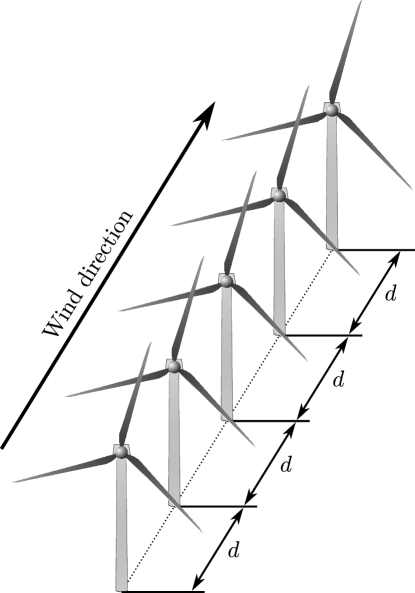
Figure 1: Simulation setup with five equidistantly arranged wind turbines.

Controller types

We compare the DR-MPC to an open-loop Scheduler that assigns a constant power references $P^{\mathrm{wt}}_{i,\mathrm{ref}}=3\>\mathrm{MW}$ for each wind turbine $i=1,\ldots,N_{\mathrm{wt}}$ for the entire simulation horizon of $T=900$ s, i.e., the wind farm should nominally produce $P^{\mathrm{wf}}_{\mathrm{ref0}}=15\>\mathrm{MW}$. In addition, we consider the SWF controller Grunnet et al. (2010), which dynamically distributes the power references based on the available wind power estimates of each wind turbine

$$P_{i,\mathrm{avail}}=\min\left\{P_{\mathrm{0}},\frac{1}{2}\pi\rho R^{2}\tilde{w}_{i}^{3}C^{\mathrm{max}}_{\mathrm{p}}\right\}\quad\forall i\in\{1,\ldots,N_{\mathrm{wt}}\},$$

where $\tilde{w}_{i}$ is the measured (effective) wind speed at turbine $i$, $P_{\mathrm{0}}$ the rated power and $C^{\mathrm{max}}_{\mathrm{p}}=0.45$ the maximum power coefficient. Therefore, the SWF controller distributes the power as follows

$$P^{\mathrm{wt}}_{i,\mathrm{ref}}=\max\left\{0,\min\bigg{\{}P_{\mathrm{0}},\frac{P^{\mathrm{wf}}_{\mathrm{ref0}}P_{i,\mathrm{avail}}}{\sum_{i=1}^{N_{\mathrm{wt}}}P_{i,\mathrm{avail}}}\bigg{\}}\right\}$$

for all $i=1,\ldots,N_{\mathrm{wt}}$.

Performance metrics

Similar to Riverso et al. (2016), we use the following metrics to evaluate the performance of each controller:

• Tracking $\displaystyle J_{\mathrm{p}}=\sqrt{\frac{1}{T}\sum_{k=0}^{T-1}\sum_{i=1}^{N_{\mathrm{wt}}}\frac{(P_{i,\mathrm{out}}(k)-P^{\mathrm{wt}}_{i,\mathrm{ref}}(k))^{2}}{N_{\mathrm{wt}}P_{\mathrm{0}}}}$,

• Shaft fatigue $\displaystyle J_{\mathrm{s}}=\mathrm{std}\left(\frac{\sum_{k=0}^{T-1}\sum_{i=1}^{N_{\mathrm{wt}}}T_{i,\mathrm{s}}(k)}{N_{\mathrm{wt}}T_{\mathrm{s0}}}\right)$,

• Tower fatigue $\displaystyle J_{\mathrm{t}}=\mathrm{std}\left(\frac{\sum_{k=0}^{T-1}\sum_{i=1}^{N_{\mathrm{wt}}}F_{i,\mathrm{t}}(k)}{N_{\mathrm{wt}}T_{\mathrm{t0}}}\right)$,

where $P_{i,\mathrm{out}}$, $T_{i,\mathrm{s}}$ and $F_{i,\mathrm{t}}$ denote the power output, main shaft torque and tower bending force of WT $i$, while $T_{\mathrm{s0}}=2.5\cdot 10^{6}$ and $T_{\mathrm{t0}}=0.27\cdot 10^{6}$ are standardization constants. To reduce the tuning effort of the MPC cost function, we fix the output weight $\bar{Q}_{\mathrm{y}}$ to

$$\bar{Q}_{\mathrm{y}}=I_{N+1}\otimes\mathrm{diag}\left(\begin{bmatrix}\frac{1}{F_{\mathrm{t0}}^{2}N}&0\\ 0&\frac{100}{T_{\mathrm{s0}}^{2}N}\end{bmatrix},\ldots,\begin{bmatrix}\frac{1}{F_{\mathrm{t0}}^{2}N}&0\\ 0&\frac{100}{T_{\mathrm{s0}}^{2}N}\end{bmatrix}\right)$$

and, analogously, the input weighting matrix to

$$\bar{R}=I_{N}\otimes\begin{bmatrix}\frac{r}{P^{2}_{\mathrm{0}}N}&\cdots&0\\ \vdots&\ddots&\vdots\\ 0&\cdots&\frac{r}{P^{2}_{\mathrm{0}}N}\end{bmatrix},$$

where $r\in\mathbb{R}_{>0}$. Thus, it remains to tune the parameter $r$, which introduces a trade-off between tracking performance and fatigue load reduction. We consider a prediction horizon of $N=5$ seconds for each simulation.

Operation scenario

We consider a realistic wind farm operation scenario in which some wind turbines temporarily operate in the below rated region due to deficiencies in wind speed, while others operate in the above rated region, cf. Morgan et al. (2011). The wind field has a mean velocity of $w_{\mathrm{0}}~{}=~{}12~{}\mathrm{m/s}$ and a turbulence intensity of $T_{\mathrm{I}}=0.1$, yielding a turbulence variance of $\sigma^{2}_{\mathrm{w}}=1.44$. For the DR-MPC, we identify during the offline phase for each wind turbine an ARMA model based on an independent wind scenario (training data) of $1000$ time steps, i.e., $N_{s}=1000$ samples. We identified both an ARMA$(2,1)$ and an ARMA$(3,2)$ model and chose the latter due to its lower root mean square error between the ARMA prediction and the training data.

In view of (Mark and Liu, 2023, Prop. 1), we derive an ambiguity radius of $\kappa^{(w_{\mathrm{0}},T_{\mathrm{I}})}_{\beta}=2.36$ with a confidence of $1-\beta=0.95$, while the empirical covariance matrix of the ARMA residuals is given by

$$\hat{\Sigma}_{\epsilon}^{(12,0.1)}=\mathrm{diag}(0.255,\>0.270,\>0.288,\>0.262,\>0.274).$$

We constrain the input deviations to $\pm 1\>\mathrm{MW}$ around the nominal operating point of $3\>\mathrm{MW}$ with a probability of $90\%$, which allows the DR-MPC to dynamically dispatch the power references depending on the available wind speed, while ensuring a power tracking goal and minimizing fatigue load. This is enforced with the input chance constraint (14e), while in addition a penalty term $5\lambda^{2}$ is added to the cost function (14a), which enforces that the interpolated initial constraint (14d) favors the feedback initialization.

4.1 Simulation results

In Table 4.1, we compare the performance of each controller regarding tracking accuracy, tower fatigue and transmission shaft fatigue, where the Scheduler is considered to be the baseline, i.e., $100\%$. Numbers below $100\%$ indicate a relative increase in performance, while numbers above $100\%$ reflect a relative decrease in performance. In particular, for $r=1$, we increase the tracking performance compared to the scheduler by approximately $52.6\%$ and compared to the SWF controller by $4.4\%$. The tracking performance increase comes at the price of increasing the tower fatigue by $27.8\%$, while reducing the main shaft fatigue by $10\%$. A reasonable choice is $r=500$, which only marginally increases the mechanical stress on the tower, while still increasing the tracking performance by nearly $34\%$.

In Figure 2, we illustrate the electrical power output of each wind turbine. First, a wake turbulence can be observed through the wind farm that causes the power output of the downstream turbines to temporarily fall below the nominal value of $3\mathrm{MW}$, e.g., at time $t~{}\approx~{}50$ the second turbine experiences a wind speed deficit that causes the power output to fall below the nominal value, while at time $t\approx 95$ the wake turbulence affects turbine five. This illustrates the weakness of the open-loop scheduler, as there is no immediate feedback to increase the output of the upstream turbines and compensate for the loss of the others. The SWF controller and the DR-MPC are both feedback strategies, which dynamically allocate power references, i.e., turbine one increases its power output as soon as the downstream turbines drop below their nominal value. This immediately results in an increase in tracking performance, but also additional mechanical fatigue. Compared to the SWF controller, the DR-MPC allows for systematically balancing the tracking performance with the increasing mechanical fatigue, which can be seen in less variance in the electrical output among all turbines.

The DR-MPC optimization problem (14) is implemented with Yalmip Lofberg (2004) and Mosek ApS (2022), and is solved in $35.6$ ms on average on an Intel i7-9700k processor with 16gb ram, confirming real-time capability as the controller should typically operate in the seconds range Spudić et al. (2015).

Table 1: Performance comparison for different controller types/parameterizations.

Method	$J_{\mathrm{p}}$	$J_{\mathrm{t}}$	$J_{\mathrm{s}}$
Scheduler	$0.0999$	$0.3217$	$0.0734$
SWF controller	$51.79\%$	$131.99\%$	$90.15\%$
DR-MPC $R=1$	$47.38\%$	$127.85\%$	$89.99\%$
DR-MPC $R=500$	$65.79\%$	$105.30\%$	$93.41\%$
DR-MPC $R=10^{3}$	$84.07\%$	$101.88\%$	$93.67\%$
DR-MPC $R=10^{4}$	$98.55\%$	$100.12\%$	$99.21\%$

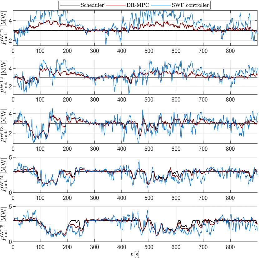
Figure 2: Wind turbine electrical power output. The DR-MPC uses the weight $r=500$.

5 Conclusion

In this paper, we presented a distributionally robust MPC approach to tackle the problem of coordinating individual wind turbines inside of a wind farm. The main objective hereby was to ensure power tracking, while a secondary goal was to reduce the mechanical stress acting on the tower and main transmission shaft. In a case study of five wind turbines in a row, we numerically verified the increase in tracking performance as well as the reduction in mechanical fatigue compared to a simple open-loop scheduler approach. In addition, we illustrated the trade-off between power tracking and fatigue reduction. We considered an ARMA model to predict the turbulent wind speed locally for each wind turbine individually, neglecting the broader picture of spatial correlations of the wind field. This can be improved by considering a spatio-temporal wind speed forecast that includes wind measurements from neighboring turbines, e.g., as proposed by Zhu et al. (2018). This could further increase the tracking performance, i.e., when a wind deficit is measured at an upstream turbine, it is inevitably passed on to the downstream turbines, allowing us to anticipate the temporary drop in output power in the future. Therefore, the output of the unaffected wind turbines can be increased to compensate for the loss of output power of the others.

References

• Andersson et al. (2021) Andersson, L.E., Anaya-Lara, O., Tande, J.O., Merz, K.O., and Imsland, L. (2021). Wind farm control-Part I: A review on control system concepts and structures. IET Renewable Power Generation, 15(10), 2085–2108.
• ApS (2022) ApS, M. (2022). The MOSEK optimization toolbox for MATLAB manual. Version 10.0. URL http://docs.mosek.com/9.0/toolbox/index.html.
• Barthelmie et al. (2007) Barthelmie, R.J., Frandsen, S.T., Nielsen, M., Pryor, S., Rethore, P.E., and Jørgensen, H.E. (2007). Modelling and measurements of power losses and turbulence intensity in wind turbine wakes at Middelgrunden offshore wind farm. Wind Energy: An International Journal for Progress and Applications in Wind Power Conversion Technology, 10(6), 517–528.
• Barthelmie et al. (2010) Barthelmie, R.J., Pryor, S.C., Frandsen, S.T., Hansen, K.S., Schepers, J., Rados, K., Schlez, W., Neubert, A., Jensen, L., and Neckelmann, S. (2010). Quantifying the impact of wind turbine wakes on power output at offshore wind farms. Journal of Atmospheric and Oceanic Technology, 27(8), 1302–1317.
• Boersma et al. (2019) Boersma, S., Doekemeijer, B.M., Keviczky, T., and van Wingerdenl, J. (2019). Stochastic model predictive control: uncertainty impact on wind farm power tracking. In Proc. American Control Conf. (ACC), 4167–4172. IEEE.
• Bossuyt et al. (2017) Bossuyt, J., Howland, M.F., Meneveau, C., and Meyers, J. (2017). Measurement of unsteady loading and power output variability in a micro wind farm model in a wind tunnel. Experiments in Fluids, 58(1), 1–17.
• Box et al. (2015) Box, G.E., Jenkins, G.M., Reinsel, G.C., and Ljung, G.M. (2015). Time series analysis: forecasting and control. John Wiley & Sons.
• Calafiore and Ghaoui (2006) Calafiore, G.C. and Ghaoui, L.E. (2006). On distributionally robust chance-constrained linear programs. Journal of Optimization Theory and Applications, 130(1), 1–22.
• Evans et al. (2014) Evans, M.A., Cannon, M., and Kouvaritakis, B. (2014). Robust MPC tower damping for variable speed wind turbines. IEEE Transactions on Control Systems Technology, 23(1), 290–296.
• Farina et al. (2013) Farina, M., Giulioni, L., Magni, L., and Scattolini, R. (2013). A probabilistic approach to model predictive control. In Proc. 52nd IEEE Conference on Decision and Control (CDC), 7734–7739. IEEE.
• Gros and Schild (2017) Gros, S. and Schild, A. (2017). Real-time economic nonlinear model predictive control for wind turbine control. International Journal of Control, 90(12), 2799–2812.
• Grunnet et al. (2010) Grunnet, J.D., Soltani, M., Knudsen, T., Kragelund, M.N., and Bak, T. (2010). Aeolus toolbox for dynamics wind farm model, simulation and control. In Proc. European Wind Energy Conf. and Exhibition (EWEC).
• Knudsen et al. (2015) Knudsen, T., Bak, T., and Svenstrup, M. (2015). Survey of wind farm control-power and fatigue optimization. Wind Energy, 18(8), 1333–1351.
• Köhler and Zeilinger (2022) Köhler, J. and Zeilinger, M.N. (2022). Recursively feasible stochastic predictive control using an interpolating initial state constraint. IEEE Control Systems Letters.
• Lofberg (2004) Lofberg, J. (2004). YALMIP: A toolbox for modeling and optimization in MATLAB. In Proc. IEEE Int. Conf. on Robotics and Automation (IEEE Cat. No. 04CH37508), 284–289. IEEE.
• Mark and Liu (2023) Mark, C. and Liu, S. (2023). Recursively Feasible Data-Driven Distributionally Robust Model Predictive Control With Additive Disturbances. IEEE Control Systems Letters, 7, 526–531.
• Morgan et al. (2011) Morgan, E.C., Lackner, M., Vogel, R.M., and Baise, L.G. (2011). Probability distributions for offshore wind speeds. Energy Conversion and Management, 52(1), 15–26.
• Ono et al. (2013) Ono, M., Topcu, U., Yo, M., and Adachi, S. (2013). Risk-limiting power grid control with an arma-based prediction model. In Proc. Conf. on Decision and Control, 4949–4956. IEEE.
• Riverso et al. (2016) Riverso, S., Mancini, S., Sarzo, F., and Ferrari-Trecate, G. (2016). Model predictive controllers for reduction of mechanical fatigue in wind farms. IEEE Transactions on Control Systems Technology, 25(2), 535–549.
• Spudić (2012) Spudić, V. (2012). Coordinated optimal control of wind farm active power. Ph. D. dissertation, Fak. elektrotehnike i računarstva, Sveučilište u Zagrebu.
• Spudić et al. (2015) Spudić, V., Conte, C., Baotić, M., and Morari, M. (2015). Cooperative distributed model predictive control for wind farms. Optimal Control Applications and Methods, 36(3), 333–352.
• Spudić et al. (2011) Spudić, V., Jelavić, M., and Baotić, M. (2011). Wind turbine power references in coordinated control of wind farms. Automatika, 52(2), 82–94.
• Van Parys et al. (2015) Van Parys, B.P., Kuhn, D., Goulart, P.J., and Morari, M. (2015). Distributionally robust control of constrained stochastic systems. IEEE Transactions on Automatic Control, 61(2), 430–442.
• Zhang and Ohtsuka (2020) Zhang, J. and Ohtsuka, T. (2020). Stochastic Model Predictive Control Using Simplified Affine Disturbance Feedback for Chance-Constrained Systems. IEEE Control Systems Letters, 5(5), 1633–1638.
• Zhu et al. (2018) Zhu, Q., Chen, J., Zhu, L., Duan, X., and Liu, Y. (2018). Wind speed prediction with spatio–temporal correlation: A deep learning approach. Energies, 11(4), 705.