Single Qubit Error Mitigation by Simulating Non-Markovian Dynamics

Abstract

Quantum simulation is a powerful tool to study the properties of quantum systems. The dynamics of open quantum systems are often described by Completely Positive (CP) maps, for which several quantum simulation schemes exist. We present a simulation scheme for open qubit dynamics described by a larger class of maps: the general dynamical maps which are linear, hermitian preserving and trace preserving but not necessarily positivity preserving. The latter suggests an underlying system-reservoir model where both are entangled and thus non-Markovian qubit dynamics. Such maps also come about as the inverse of CP maps. We illustrate our simulation scheme on an IBM quantum processor by showing that we can recover the initial state of a Lindblad evolution. This paves the way for a novel form of quantum error mitigation. Our scheme only requires one ancilla qubit as an overhead and a small number of one and two qubit gates.

Introduction.- Quantum computing has created a computational paradigm that may lead to the development of new and powerful solutions to computational tasks. A prominent application of digital quantum computers is their ability to simulate other quantum systems, already on the level of noisy intermediate scale (NISQ) quantum platforms Georgescu et al. (2014).

Although there already exists a wide range of quantum simulation methods for closed quantum systems, see e.g. Lloyd (1996); Berry et al. (2006); Childs (2009); Wiebe et al. (2011), the simulation of an open quantum system is a more arduous task. Since it is often not possible to simulate the complete system plus environment dynamics, simulation methods mainly focus on realizing the reduced effective dynamics of the open quantum system.

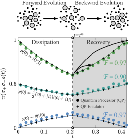
Figure 1: (Top) Reversing the direction of time of a dissipative system brings it back to its initial state. (Bottom) We recover the initial state of a Lindblad evolution (Single Qubit Error Mitigation by Simulating Non-Markovian Dynamics) by simulating its time-reversed evolution $\frac{d}{dt}\rho_{t}=-\mathcal{L}_{t}(\rho_{t})$, for different initial states. For $t\leq t^{*}$ the points show the forward evolution simulated on an IBM quantum computer, for $t>t^{*}$ the backward evolution. The lines are the numerical integration of the master equations (Single Qubit Error Mitigation by Simulating Non-Markovian Dynamics) and their time-reversed versions. $\mathcal{F}$ gives the fidelity between the final recovered state and the initial state. The parameters of the master equations are $\beta=\omega=\gamma=1$.

To find reduced descriptions for the evolution of open quantum systems, one typically assumes that system and environment are initially in a product state. In this case, the evolution is guaranteed to be described by a Completely Positive (CP) map Rivas and Huelga (2012) acting on the initial system state, which can be obtained by resorting to numerical methods (such as Strathearn et al. (2018); Suess et al. (2014); Prior et al. (2010); Tanimura and Kubo (1989); Xu et al. (2022)) or perturbative schemes Breuer and Petruccione (2002). A CP map is said to be CP-divisible if it can be divided into small arbitrary parts that are themselves CP. In this case, the evolution of the system can be described by the Lindblad-Gorini-Kossakowski-Sudarshan equation Lindblad (1976); Gorini et al. (1976). When a significant amount of entanglement accumulates between the system and the environment, the use of CP maps no longer makes sense Rivas (2020).

Quantum simulation methods for Lindblad-like dynamics have been extensively studied Bacon et al. (2001); Lloyd and Viola (2001); Weimer et al. (2010); Wang et al. (2011); Kliesch et al. (2011); Barthel and Kliesch (2012) and experimentally implemented Schindler et al. (2013). Recently the authors of Guimarães et al. (2023) simulated Lindbladian dynamics on an IBM quantum processor by exploiting error mitigation. An efficient simulation scheme for any CP qubit map was developed by Wang et al. (2013), based on the results of King and Ruskai (2001); Ruskai et al. (2002). The scheme by Wang et al. (2013) uses a single ancillary qubit, single qubit rotations and CNOT gates and was experimentally realised on a superconducting circuit Han et al. (2021).

In this Letter we propose a novel simulation scheme for general qubit dynamical maps going beyond CP divisible maps King and Ruskai (2001); Ruskai et al. (2002); Wang et al. (2013). General dynamical maps are trace-preserving and hermicity-preserving, but not necessarily positivity-preserving. They naturally arise as the inverse of CP maps, and thus the ability to simulate them allows to revert noise effects on the system. In Fig. 1 we recover several initial states of a qubit disturbed by a thermal Lindblad equation on an IBM quantum processor. General dynamical maps also arise in the context of general time-local master equations in which the initial state is not assumed to be in a product state, but has already created some system-bath entanglement. Their derivation is based on tracing out environmental degrees of freedom in Gaussian boson Feynman and Vernon (1963); Karrlein and Grabert (1997), fermion Tu and Zhang (2008); Donvil et al. (2020) or other exactly solvable models John and Quang (1994), or via time convolutionless perturbation theory methods Hashitsumae et al. (1977); Breuer and Petruccione (2002).

For our proposed scheme, we exploit the fact that general dynamical maps acting on finite dimensional systems can always be decomposed as the difference of two CP maps Sweke et al. (2016); Rossini et al. . We demonstrate that the decomposition can be brought into a suitable form for quantum simulations, namely, as a weighted difference of two completely positive trace-preserving (CPTP) maps.

Another, more general avenue for the simulation of open quantum systems on a quantum computer are collision methods Ciccarello et al. (2022); Cattaneo et al. (2021). Here the open quantum system repeatedly interacts or ”collides” with ancillary systems. Non-Markovian dynamics can be implemented by allowing the ancillas to interact amongst themselves in between system-ancilla collisions McCloskey and Paternostro (2014); Lorenzo et al. (2016); Kretschmer et al. (2016). Such models were successfully implemented on IBM quantum processors Guillermo García-Pérez and Maniscalco (2020). Other methods for quantum simulation of open quantum systems have been proposed in the context of non-equilibrium systems Lamm and Lawrence (2018) and quantum thermodynamics Jin-Fu Chen and Dong (2021).

In contrast to collision-based methods such as McCloskey and Paternostro (2014); Lorenzo et al. (2016); Kretschmer et al. (2016), the main advantage of the algorithm we present here is its problem-agnostic applicability. No specific design is required for each dynamics one aims to simulate. In fact, we are able to simulate the dynamics of a given system from any point in time to any later time, whereas collision-based methods require the protocol to always start from the initial time of the evolution and rely on the Trotterization of the dynamics. As an additional benefit, our proposed scheme is resource efficient as the computational overhead does not grow with the simulated time.

We illustrate these features by implementing two paradigmatic examples on IBM quantum processors which demonstrate the ability to simulate the time evolution from any intermediate point in time, even when the evolution map is not CP and the ability to recover the initial state of a Lindbladian evolution Donvil and Muratore-Ginanneschi (2022), see Fig. 1.

This last example shows that one of the promising applications of the new scheme is to perform error mitigation on a NISQ platform by recovering the typically unknown undisturbed initial state.

Theoretical framework.- A finite dimensional linear map $\Lambda$ is CP if and only if its action on a state $\rho$ can be written in terms of a set of matrices $\{K_{j}\}_{j}$, often referred to as Kraus operators: $\Lambda(\rho)=\sum_{j}K_{j}\rho K_{j}^{\dagger}$. The map is trace preserving iff. $\sum_{j}K_{j}^{\dagger}K_{j}=\mathbb{I}$, where $\mathbb{I}$ is the identity on the appropriate Hilbert space, see e.g. Breuer and Petruccione (2002); Rivas and Huelga (2012). The results of King and Ruskai (2001); Ruskai et al. (2002) prove that any CPTP qubit map $\Lambda$ is equal to the convex sum of two extremal CP maps $\Lambda_{1}$ and $\Lambda_{2}$ that are both realised by a pair of Kraus operators. Concretely, they showed that for every CPTP qubit map $\Lambda$ there exist two pairs of unitaries $U_{j}$, $V_{j}$ and two pairs of Kraus operators $F_{i,j}$ (with $i,j\in\{1,2\}$) defining the extremal maps

$$\Lambda_{j}(\rho)=U_{j}\left(\sum_{i=1}^{2}F_{i,j}(V_{j}\rho V_{j}^{\dagger})F_{i,j}^{\dagger}\right)U_{j}^{\dagger}$$ (1)

such that

$$\Lambda(\rho)=\frac{1}{2}\Lambda_{1}(\rho)+\frac{1}{2}\Lambda_{2}(\rho).$$ (2)

The authors of Wang et al. (2013) devised a simple circuit shown in Fig. 2 (b) to realise the action of the $\Lambda_{j}$ using just one ancillary qubit and CNOT gates.

General dynamical maps are linear, trace-preserving and self-adjoint but not necessarily positivity preserving. For finite dimensional systems such maps can always be written as the difference of two CP maps Rossini et al.

$$\Sigma(\rho)=\Lambda_{+}(\rho)-\Lambda_{-}(\rho)=\sum_{j}K_{j}\rho K_{j}^{\dagger}-\sum_{j}M_{j}\rho M_{j}^{\dagger}.$$ (3)

The map $\Sigma$ is trace preserving under the condition $\sum_{j}K_{j}^{\dagger}K_{j}-\sum_{j}M_{j}^{\dagger}M_{j}=\mathbb{I}$. Since $\Lambda_{\pm}$ are bounded, there exists a positive number $p$ such that $\sum_{j}M_{j}^{\dagger}M_{j}\leq p\,\mathbb{I}$. We define the semi-positive definite operator $D=\sqrt{p\,\mathbb{I}-\sum_{j}M_{j}^{\dagger}M_{j}}$ and write

$$\Sigma(\rho)=(1+p)\Lambda^{*}_{+}-p\Lambda^{*}_{-},$$ (4)

where $\Lambda^{*}_{+}=\frac{\sum_{j}K_{j}\rho K_{j}^{\dagger}+D\rho D^{\dagger}}{1+p}$ and $\Lambda^{*}_{-}=\frac{\sum_{j}M_{j}\rho M_{j}^{\dagger}+D\rho D^{\dagger}}{p}$. It is straightforward to check that both maps $\Lambda^{*}_{\pm}$ are trace preserving and CP. The above equation is our first main result. It shows that any general dynamical map $\Sigma$ can be decomposed as the weighted difference of two CPTP maps. The above decomposition is an alternative to the decomposition in terms of CPTP maps by Sudarshan and Shaji (2003) which involves applying positive, non-unitary transformations to the quantum state. The latter makes our decomposition more attuned for simulating the action of $\Sigma$ on an experimental platform.

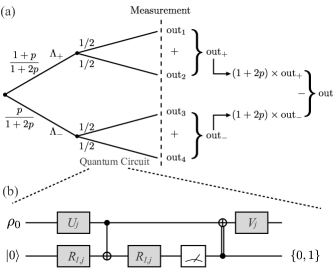
Figure 2: (a) Representation of the algorithm simulating general dynamical maps decomposed as the weighted difference of two CPTP maps 4. At each branching point a choice is made with a classical random number generator with the indicated probability. At the dashed line, the measurement of some observable is performed. Finally, the outcomes are rescaled and subtracted from one another. (b) The circuit by Wang et al. (2013) to realise the extremal maps (2).

.

Algorithm and circuit schemes.- The simulation scheme we propose for general dynamical maps is illustrated in Fig. 2(a). First, a classical random number generator is used to choose the branch $\Lambda_{+}^{*}$ or $\Lambda_{-}^{*}$ corresponding to equation (4), with probabilities $\frac{1+p}{1+2p}$ and $\frac{p}{1+2p}$, respectively. Then one of the two extremal maps (2) is selected with probability 1/2 and realized by the circuit representation for the extremal maps of Wang et al. (2013) shown in Fig. 2(b). Next, a measurement of an observable is performed and the outcomes within the plus and minus branch are summed. Finally, the measurement result is rescaled by $1+2p$ to restore normalization, and the results of both branches are subtracted.

The scheme depicted in Fig. 2 can be straightforwardly be implemented on a quantum computational platform. Particularly, we use the Ehningen IBM quantum device. Generating the dynamics of a system using the algorithm described above requires eight different quantum circuits as shown in Fig.2(b). Every circuit requires single-qubit unitary gates $U_{j}$, $V_{j}$, $R_{1,j}$ and $R_{2,j}$, which we construct explicitly in Rossini et al. , are realized via a universal set of single-qubit gates. Beyond single-qubit unitary gates, CNOT gates and a measurement operation on the ancilla are performed. With this circuit representation any single qubit map $\Lambda$ can be simulated with an error $\leq\varepsilon$ using a computer time of $O(\textrm{polylog}(1/\varepsilon))$ Wang et al. (2013).

In order to minimize the noise effects of the quantum device, we implemented standard methods of quantum error mitigation Rossini et al. . We select the qubits and connections on the platform showing the least error rate for each circuit implementation and optimise the specific gate protocol to minimise the number CX gates, being most prone to generate errors. We make use of readout error mitigation with an exploratory run on the device to uncover its systematic readout error and apply this to correct the measurement results.

The data points in Figs. 1 and 4 are each averaged over ten runs of each 10000 shots, i.e. 10000 circuits are implemented according to the probability distribution in Fig. 2(a). Errors bars are within the size of the data points. Therefore, the final infidelity is mostly due to systematic errors in the quantum gates and the measurement scheme within a specific circuit calibration .

Simulating General Time Local Master Equations.- General trace-preserving time-local master equations are of the form

$$\frac{d}{dt}\rho_{t}=\mathcal{L}_{t}(\rho_{t})$$

$$=-i[H_{t},\rho_{t}]+\sum_{k}\Gamma_{k,t}(L_{k}\rho_{t}L_{k}^{\dagger}-\frac{1}{2}\{L_{k}^{\dagger}L_{k},\rho_{t}\}),$$ (5)

where the $L_{k}$ are operators and the $\Gamma_{k}(t)$ are scalar weight functions. The above equation has the appearance of a Lindblad equation except for the fact that the weight functions $\Gamma_{k}(t)$ are not assumed to be positive definite. General time-local master equations describe the evolution of a wide class of open quantum systems, as they can be derived from the Nakajima-Zwanzig equation Zwanzig (2001) when its solution has an inverse that exists during a finite time interval Vstovsky (1973); Grabert et al. (1977); van Wonderen and Lendi (1995); Andersson et al. (2007); Chruściński and Kossakowski (2010). For an initial condition $\rho_{0}$ the formal solution of (Single Qubit Error Mitigation by Simulating Non-Markovian Dynamics) is $\rho_{t}=\Lambda_{t,0}(\rho_{0})=T\exp\left(\int_{0}^{t}ds\,\mathcal{L}_{s}\right)\rho_{0}$, where the map $\Lambda_{t,0}$ is guaranteed to be CP if the underlying system-environment model is in a product state.

The master equation (Single Qubit Error Mitigation by Simulating Non-Markovian Dynamics) generates maps that satisfy the semi-group property: For $\Lambda_{t,s}$ being the map that evolves a state from time $s$ to time $t$, then $\Lambda_{t,s}=\Lambda_{t,u}\Lambda_{u,s}$ for $t\geq u\geq s$. This property is very convenient since we can split up the evolution into smaller segments that evolve the density matrix from one time to the next. However, complete positivity of $\Lambda_{t,0}$ does not necessarily guarantee that all intermediate maps $\Lambda_{s,u}$ are CP. In fact, if this is the case, all weights $\Gamma_{k,t}$ are positive definite and (Single Qubit Error Mitigation by Simulating Non-Markovian Dynamics) reduces to the conventional Lindblad form.

If intermediate $\Lambda_{u,s}$ are not positivity preserving, this implies that not all quantum states are mapped into quantum states, i.e. some quantum states are mapped into operators with negative eigenvalues. Indeed, weight factors $\Gamma_{k,t}$ taking negative values capture an underlying system-environment model with meaningful entanglement built up between them. In this case, the reduced system state operator at an instant of time is no longer sufficient to describe the subsequent time evolution, as one requires knowledge of the history of the system-environment interaction.

To illustrate this, we consider a qubit master equation with four operators and their respective weight functions, i.e. $L_{1}=\sigma_{-}$, $L_{2}=\sigma_{+}$, $L_{3}=\tau_{-}$ and $L_{4}=\tau_{+}$ with $\sigma_{\pm}$ being the raising and lowering operators of $\sigma_{z}$ and $\tau_{\pm}$ of $\sigma_{x}$, respectively. As weight factors we choose a typical non-Markovian model with oscillations to negative values that exponentially decay, which mimics resonance with an environmental mode Breuer et al. (2016). Figure 3 displays these weight functions, where the grey zone indicates the times at which they are all negative. If the evolution of the density according to (Single Qubit Error Mitigation by Simulating Non-Markovian Dynamics) starts in this time interval, for short times it will not be positivity preserving. Therefore, the solution of the master equation from these times has to be described within the above framework of general dynamical map.

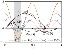
Figure 3: Weight functions of the time local master equation (Single Qubit Error Mitigation by Simulating Non-Markovian Dynamics). The rates are of the form $\Gamma_{j}(t)=a_{j}\exp(-t)(b_{j}-\sin^{2}(c_{j}\pi t))-d_{j}$, with $a_{2}=a_{3}=1$, $a_{1}=3$ and $a_{4}=1.5$; $b_{1}=4.5$, $b_{2}=3.5$, $b_{3}=1$ and $b_{4}=1.5$; $c_{1}=2$, $c_{2}=2$, $c_{3}=2.3$ and $c_{4}=2.2$, $d_{1}=d_{2}=2.6$ and $d_{3}=d_{4}=0.4$

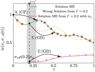
Figure 4: Excited state population according to solutions of (Single Qubit Error Mitigation by Simulating Non-Markovian Dynamics) (lines) and IBM simulations (symbols), for an initial state $\rho_{0}=(1+\sigma_{z})/2$. In the shaded region all weights are negative, so the evolution starting from there is ensured to be non-positivity preserving. The dynamical map $\Lambda_{t,0}$ is CP, while starting at a later time $t^{\prime}=0.2$, the map $\Sigma\equiv\Lambda_{t,t^{\prime}}$ is only ensured to be a general dynamical map. The (yellow) line shows the evolution of the state from time $t^{\prime}=0.2$ when forgetting about the past interaction with the environment. The purple line (green triangles) show the evolution from $t^{\prime}=0.20$ after the unitary transformation $\sigma_{x}$ was applied to the state.

The excited state population according to (Single Qubit Error Mitigation by Simulating Non-Markovian Dynamics) is shown in Fig. 4. Results obtained with the CP map $\Lambda_{t,0}[\rho_{0}]$ with $\rho_{0}=(1+\sigma_{z})/2$ are shown as (green) full line for a direct integration of (Single Qubit Error Mitigation by Simulating Non-Markovian Dynamics) together with those from simulations on the IBM device (squares) following the recipe outlined above. Starting at the intermediate time $t^{\prime}=0.2$ in the grey area of Fig. 3, diamonds display IBM simulations with the general dynamical map $\Sigma\equiv\Lambda_{t,t^{\prime}}[\rho_{t^{\prime}}]$. Since at $t^{\prime}$ all weight functions are negative definite, the solution (for short times, at least) is not CP. In contrast, when forgetting about the past interaction with the environment according to an evolution with $\Lambda_{t-t^{\prime},0}[\rho_{t^{\prime}}]$ (dashed yellow), the correct dynamics of (Single Qubit Error Mitigation by Simulating Non-Markovian Dynamics) is not recovered.

Having access to the intermediate evolution maps starting from $t^{\prime}>0$ has great advantages. For example, we are able to evolve a state from $0$ to $t^{\prime}$, perform a quantum operation on it and then evolve it further with a completely bounded evolution. The (pink) full line in Fig. 4 displays this situation after applying the unitary transformation $\sigma_{x}$ to the state at $t^{\prime}=0.2$, while the (green) triangles show the corresponding IBM simulations of the general dynamical map according to the new scheme.

Quantum State Recovery.- Another intriguing consequence of the new simulation method is that one can recover the initial state of a Lindblad evolution obtained on a quantum device by implementing its time reversed master equation Donvil and Muratore-Ginanneschi (2022). Concretely, we consider a master equation for a qubit weakly coupled to a thermal reservoir $\frac{d}{dt}\rho_{t}=\mathcal{L}_{t}(\rho_{t})$ with

$$\mathcal{L}_{t}(\rho_{t})= -i\omega[\sigma_{z}/2,\rho_{t}]+\gamma e^{\beta\omega}(\sigma_{-}\rho\sigma_{+}\frac{1}{2}\{\sigma_{+}\sigma_{-},\rho_{t}\})$$

$$+\gamma(\sigma_{+}\rho\sigma_{-}\frac{1}{2}\{\sigma_{-}\sigma_{+},\rho_{t}\})$$ (6)

and its time reversed evolution $\frac{d}{dt}\rho_{t}=-\mathcal{L}_{t}(\rho_{t})$.

Thus, evolving a state for a time $t$ with (Single Qubit Error Mitigation by Simulating Non-Markovian Dynamics) and then for a time $s\leq t$ with its time reversed evolution results in the state obtained by just evolving with (Single Qubit Error Mitigation by Simulating Non-Markovian Dynamics) for a time $t-s$. We implement both the forwards and backwards evolution on the IBM device with our simulation scheme (4).

In Fig. 1 data points for $t\leq t^{*}$ and various initial states reflect the thermalization dynamics of (Single Qubit Error Mitigation by Simulating Non-Markovian Dynamics). At $t=t^{*}$ the recovery sets in to approach earlier states in the dissipative time evolution. Note that the recovery is performed by mapping the state $\rho(t=t^{*})$ directly to each recovered state with only one algorithm run per state.

Outlook.- We have shown that the class of general qubit dynamical maps can be straightforwardly simulated using just four extremal CP maps each consisting of two pairs of Kraus operators. Environmental noise on a quantum system is generally described by a CP map. As the inverse of a CP map is a general dynamical map, one of the promising applications of our simulation scheme is to perform error mitigation by recovering the typically unknown bare qubit state in absence of any environmental coupling. We prove the viability of this in Fig. 1 on an IBM quantum processor. A next step is to determine the noise CP map of a single qubit of a quantum processor and to revert it using our simulation scheme and thus performing genuine quantum error mitigation.

Acknowledgements

We thank P. Muratore-Ginanneschi, M. Donvil and J. Stockburger for valuable discussions. Financial support through the WM-BW within the Quantum Computing Competence Network BW (SiQuRe), the BMBF within QSens (QComp), and QSolid (BMBF) is gratefully acknowledged.

I Supplemental Material

The authors of Wang et al. (2013) present a simple simulation scheme for completely positive trace preserving qubit maps, i.e. qubit channels. Recently, the protocol was realised experimentally by Han et al. (2021). The method of Wang et al. (2013) relies on an earlier mathematical results by Ruskai et al. (2002); King and Ruskai (2001) which allow to write qubit channels as the convex sum of extremal channels. Concretely, these channels consist of two unitary transformations and the sum of two rather simple Kraus operators.

We are concerned with trace preserving general qubit dynamical maps. These maps are trace-preserving, self-adjoint but not necessarily positivity-preserving. Importantly, these maps can always be written as the difference of two completely positive maps. We show that here that any general dynamical map can be written as the weighted difference of two quantum channels. Combining this with the results of Ruskai et al. (2002); King and Ruskai (2001); Wang et al. (2013) we find a general simulation method for general qubit dynamics which needs just one ancilla qubit.

II General dynamical maps

Completely bounded maps are linear maps $\Lambda$ for which the trivial extensions $\Lambda_{N}=\Lambda\otimes\mathbb{I}_{N}$ to larger Hilbert spaces $\mathcal{H}\otimes\mathbb{C}_{N}$ satisfy

$$\|\Lambda\|_{cb}=\sup_{N}\|\Lambda_{N}\|<\infty.$$ (7)

All maps linear maps acting on finite dimensional systems are completely bounded Paulsen (2003). When these linear maps are trace preserving and self-adjoint we call them general dynamical maps. A physically relevant example of general dynamical maps are solutions to general time local master equations

$$\frac{d}{dt}\rho_{S}(t)=-i[H,\rho_{S}(t)]+\sum_{k}\gamma_{k}(t)\left(L_{k}\rho_{S}(t)L_{k}^{\dagger}-\frac{1}{2}\{L_{k}^{\dagger}L_{k},\rho_{S}(t)\}\right)$$ (8)

where the weights $\gamma_{k}(t)$ have no positivity requirements.

The Wittstock-Paulsen decomposition for completely bounded maps states that any completely bounded map can be written as the difference of two completely positive maps. Concretely, for every completely bounded $\Lambda$ there exist two completely positive maps $\Lambda_{\pm}$ such that

$$\Lambda=\Lambda_{+}-\Lambda_{-}.$$ (9)

where $\|\Lambda_{+}\|,\,\|\Lambda_{-}\|\leq\|\Lambda\|_{cb}$. We can write the completely positive maps in terms of Kraus operators

$$\Lambda_{+}\rho=\sum_{k}M_{k}\rho M_{k}^{\dagger},\quad\Lambda_{-}\rho=\sum_{l}K_{l}\rho K_{l}^{\dagger}.$$ (10)

If $\Lambda$ is trace preserving then

$$\sum_{k}M_{k}^{\dagger}M_{k}-\sum_{j}K_{j}^{\dagger}K_{j}=\mathbb{I}.$$ (11)

Since $\|\Lambda_{-}\|$ is bounded, there exists and $\alpha\geq\|\Lambda\|_{cb}$ such that

$$\sum_{j}K_{j}^{\dagger}K_{j}\leq p\mathbb{I}$$ (12)

Therefore the difference $p\mathbb{I}-\sum_{j}K_{j}^{\dagger}K_{j}=D^{\dagger}D$ is a positive matrix and

$$\sum_{j}K_{j}^{\dagger}K_{j}+D^{\dagger}D=p\mathbb{I}.$$ (13)

Let us now rewrite (9) as

$$\Lambda(\rho)=({1+p})\left(\frac{\Lambda_{+}(\rho)+D\rho D^{\dagger}}{1+p}\right)-p\left(\frac{\Lambda_{-}(\rho)+D\rho D^{\dagger}}{p}\right)$$ (14)

where the above equation is the weighted difference of completely positive maps. Moreso, the operators between the brackets are both trace 1.

II.1 Decomposition into completely positive maps

Let $\Sigma$ be a general dynamical map acting on a finite dimensional space. We compute the Choi matrix $C(\Sigma)$

$$C(\Sigma)=\sum_{ij}e_{ij}\otimes\Sigma(e_{ij}),$$

where $e_{ij}$ are the elementary matrices. The map $\Sigma$ can be obtained from the Choi matrix by

$$\Sigma(\rho)=\textrm{tr}_{1}(C(\Sigma)\,\rho^{\top}\otimes\mathbb{I})$$

where $\textrm{tr}_{1}$ and $\rho^{\top}$ is the transpose of $\rho$.

The Choi matrix has the property that its positivity is equivalent to the complete positivity of underlying map. Since $\Sigma$ is self-adjoint, $C(\Sigma)$ is a self-adjoint matrix and therefore diagonalisable. Let its eigenvectors and eigenvalues be $v_{i}$ and $\lambda_{i}$, we the define

$$C_{\pm}(\Sigma)=\sum_{i}\max(0,\pm\lambda_{i})\,v_{i}v_{i}^{\dagger}$$

such that

$$C(\Sigma)=C_{+}(\Sigma)-C_{-}(\Sigma).$$ (15)

We then define $\Lambda_{\pm}(\rho)$ in equation (9) as $\Lambda_{\pm}(\rho)=\textrm{tr}_{1}(C_{\pm}(\Sigma)\,\rho^{\top}\otimes\mathbb{I})$.

III Decomposition in extremal maps

The authors of Ruskai et al. (2002); King and Ruskai (2001) proved that any single qubit channel $\Lambda$ can be written as the convex sum of two channels ”belonging to the closure of the set of extreme points of single qubit channels”.

Let $\Lambda$ be a completely positive trace preserving map acting on qubit states. We can represent the action of $\Lambda$ on a state $\rho=\frac{1}{2}(\mathbb{I}+w\cdot\sigma)$ in terms of a $4\times 4$ matrix $\mathbb{T}$

$$\mathbb{T}=\begin{pmatrix}1&0\\ t&T\end{pmatrix},\quad\mathbb{T}_{ij}=\frac{1}{2}\text{tr}(\sigma_{i}\Lambda(\sigma_{j}))$$ (16)

such that

$$\Lambda(\rho)=(\mathbb{I}+(t+Tw)\cdot\sigma).$$ (17)

There then exist two unitaries $U$, $V$ and a completely positive map $\Lambda^{\prime}$ with diagonal $T$ such that

$$\Lambda(\rho)=U\Lambda^{\prime}(V\rho V^{\dagger})U^{\dagger}$$ (18)

where

$$T^{\prime}=\begin{pmatrix}\lambda_{1}&0&0\\ 0&\lambda_{2}&0\\ 0&0&\lambda_{3}\end{pmatrix}$$ (19)

For the extremal maps, $\mathbb{T}^{\prime}$ can be written as

$$\mathbb{T}^{\prime}=\begin{pmatrix}1&0&0&0\\ 0&\cos\nu&0&0\\ 0&0&\cos\mu&0\\ \sin\mu\,\cos\mu&0&0&\cos\mu\,\cos\mu\end{pmatrix}$$ (20)

The map defined by $\mathbb{T}^{\prime}$ can be obtained from just 2 Kraus operators

$$F_{0}=\begin{pmatrix}\cos\frac{\mu-\nu}{2}&0\\ 0&\sin\frac{\mu+\nu}{2}\end{pmatrix},\qquad F_{1}=\begin{pmatrix}0&\cos\frac{\mu+\nu}{2}\\ \sin\frac{\mu-\nu}{2}&0\end{pmatrix},$$ (21)

By Ruskai et al. (2002); King and Ruskai (2001) any completely positive qubit channel $\Lambda$ can be written as the convex sum of two convenient completely positive maps

$$\Lambda=\Lambda_{1}+\Lambda_{2}.$$ (22)

with

$$\Lambda_{j}(\rho)=U_{j}(F_{0,j}\,V_{j}\rho V_{j}^{\dagger}\,F^{\dagger}_{0,j}+F_{1,j}\,V_{j}\rho V_{j}^{\dagger}\,F^{\dagger}_{1,j})U_{j}^{\dagger}$$ (23)

where $V_{j}$ and $U_{j}$ are unitaries and the Kraus operators $F_{0,j}$ and $F_{1,j}$.

IV Completely Positive Maps

IV.1 Diagonal representation of completely positive maps

The action of a qubit channel on a qubit state can be expressed in terms of a 3 dimensional vector $t$ and a $3\times 3$ matrix $T$. Let $\rho=\frac{1}{2}(\mathbb{I}+w\cdot\sigma)$, then

$$\Lambda(\rho)=\frac{1}{2}(\mathbb{I}+(t+Tw)\cdot\sigma).$$

In this section, we follow King and Ruskai (2001) and show how to find a diagonal representation. We write the singular value decomposition for $T$

$$T=VDW^{\dagger}$$ (24)

where, since $T$ is a real matrix, $V$ and $W$ can be chosen to be real and thus orthogonal matrices. If $\det(V)=1$, $V$ is a rotation matrix, if $\det(V)=-1$ then $-V$ is a rotation matrix. Thus let $R_{1,2}$ are rotation matrices, then

$$T=\frac{V}{\det V}\frac{D}{(\det V)(\det W^{\dagger})}\frac{W^{\dagger}}{\det(W^{\dagger})}$$ (25)

IV.1.1 Rotation on the Bloch Sphere as a Unitary Transformation

A rotation on the Bloch sphere around the axis $\hat{n}$ with and angle $\theta$ can be represented by the unitary transformation on the Hilbert space

$$U=\exp\left(-i\theta\,\hat{n}\cdot\frac{1}{2}\vec{\sigma}\right)$$

We find the axis of a rotation matrix $R$ by solving

$$(R-\mathbb{I})\hat{n}=0$$ (26)

with $\|\hat{n}\|=1$ and the angle of rotation by

$$\text{tr}(R)=1+2\cos\theta$$ (27)

IV.1.2 Diagonal representation

We can thus write

$$\Lambda(\rho)=U_{1}\Lambda_{D}(U_{2}\rho U_{2}^{\dagger})U_{1}^{\dagger}$$

where

$$\Lambda_{D}\left(\frac{1}{2}(\mathbb{I}+w\cdot\sigma)\right)=\frac{1}{2}\left(\mathbb{I}+\left(\frac{V^{\dagger}}{\det V^{\dagger}}\,t+\frac{D}{(\det V)(\det W^{\dagger})}w\right)\cdot\sigma\right)$$

IV.2 Convex sum

I repeat here the main results of Ruskai et al. (2002) to show how a completely positive map can be written as the convex sum of two extremal maps.

Let $\Phi$ be a completely-positive trace-preserving qubit map and let $\hat{\Phi}$ be its adjoint. The Choi representation of $\hat{\Phi}$ is then a $4\times 4$ matrix of the form

$$C(\hat{\Phi})=\begin{pmatrix}\hat{\Phi}(E_{11})&\hat{\Phi}(E_{12})\\ \hat{\Phi}(E_{21})&\hat{\Phi}(E_{22})\end{pmatrix}=\begin{pmatrix}A&C\\ C^{\dagger}&\mathbb{I}-A\end{pmatrix}.$$

where $A$ and $C$ are $2\times 2$ matrices. The diagonal elements sum to one since $\hat{\Phi}(E_{11})+\hat{\Phi}(E_{22})=\hat{\Phi}(\mathbb{I})=\mathbb{I}$ by trace preservation. Furthermore, since $\hat{\Phi}(E_{11}),\,\hat{\Phi}(E_{22})\geq 0$, we have that $A\leq\mathbb{I}$. Note that the Choi matrix of $\Phi$ and $\hat{\Phi}$ are related by

$$C(\hat{\Phi})=\overline{U^{\dagger}_{23}C({\Phi})U_{23}},$$

where $U_{23}$ is the unitary matrix

$$U_{23}=U^{\dagger}_{23}=\begin{pmatrix}1&0&0&0\\ 0&0&1&0\\ 0&1&0&0\\ 0&0&0&1\end{pmatrix}.$$

Such that $C(\hat{\Phi})$ is positive definite if and only if $C(\Phi)$ positive definite is.

Lemma 1.

A matrix

$$\begin{pmatrix}A&C\\ C^{\dagger}&B\end{pmatrix}$$

is positive semi-definite if and only if $A\geq 0$, $B\geq 0$ and $C=\sqrt{A}R\sqrt{B}$ where $R$ is a contraction (i.e. $\|R\|\leq 1$).

The following proposition then tells us something about the $R$ for generalised extreme points

Proposition 1.

A map is a generalised extreme point if and only if $C(\hat{\Phi})$ is of the form

$$C(\hat{\Phi})=\begin{pmatrix}A&\sqrt{A}U\sqrt{\mathbb{I}-A}\\ \sqrt{\mathbb{I}-A}U^{\dagger}\sqrt{A}&\mathbb{I}-A\end{pmatrix}$$

where $U$ is a unitary and $0\leq A\leq\mathbb{I}$.

Lemma 2.

Let $R$ be a $2\times 2$ contraction, its singular value decomposition is of the form

$$R =V\begin{pmatrix}\cos\theta_{1}&0\\ 0&\cos\theta_{2}\end{pmatrix}W^{\dagger}$$

$$=\frac{1}{2}V\begin{pmatrix}e^{i\theta_{1}}&0\\ 0&e^{i\theta_{2}}\end{pmatrix}W^{\dagger}+\frac{1}{2}V\begin{pmatrix}e^{-i\theta_{1}}&0\\ 0&e^{-i\theta_{2}}\end{pmatrix}W^{\dagger}$$

$$=\frac{U_{1}}{2}+\frac{U_{2}}{2}$$

where $U_{1,2}$ are unitaries.

Proposition 2.

The Choi representation of the adjoint of any qubit channel $\Phi$ can be written as the convex sum of the Choi representation of two generalised extremal channels.

Proof.

We have that

$$C(\hat{\Phi}) =\begin{pmatrix}A&\sqrt{A}R\sqrt{\mathbb{I}-A}\\ \sqrt{\mathbb{I}-A}R^{\dagger}\sqrt{A}&\mathbb{I}-A\end{pmatrix}$$

$$=\frac{1}{2}\begin{pmatrix}A&\sqrt{A}U_{1}\sqrt{\mathbb{I}-A}\\ \sqrt{\mathbb{I}-A}U_{1}^{\dagger}\sqrt{A}&\mathbb{I}-A\end{pmatrix}+\frac{1}{2}\begin{pmatrix}A&\sqrt{A}U_{2}\sqrt{\mathbb{I}-A}\\ \sqrt{\mathbb{I}-A}U_{2}^{\dagger}\sqrt{A}&\mathbb{I}-A\end{pmatrix}$$

∎

V Error Mitigation

In order to obtain meaningful results from state-of-the-art NISQ quantum devices, it is necessary to employ methods aimed at mitigating the effect of noise. Among the various methods available in the field of quantum error correction and mitigation, we chose to use three methods to reduce the impact of device errors in our measurements.

The first is to transpile, i.e. the operation that translates any theoretically designed circuit into the base of gates that the quantum device can actually implement, the circuit we have designed in order to reduce errors. This can be done, for example, by reducing the amount of CX gates needed to perform the given task.

The second is to choose from the set of qubits available in the quantum processor those that, at the time of each simulation, have the best coherence properties and protection from measurement errors with regard to the circuit we want to run. This can be done using specially designed functions from the Qiskit package, which can retrieve the state of each qubit in the processor directly from IBM’s servers.

The third and slightly most refined method is readout error mitigation. Ideal measurements can be described by projection operators: each possible measurement result $i$ corresponds to a projection operator $P_{i}$, where $\sum_{i}P_{i}=I$. Performing a measurement on a quantum system in state $\rho$, the probability $p_{i}$ of obtaining result $i$ is given by $p_{i}={\rm Tr}(P_{i}\rho)$. Let us now assume that the measurement contains errors of the following kind: with probability $p_{1|0}$, the result ‘0‘ is turned into ‘1‘, and vice versa $p_{0|1}$. Although the resulting measurement is no longer projective, the basic formalism (POVM: positive operator valued measure) remains the same - except for the fact that the operators become

$$P_{0}=\left(\begin{array}[]{cc}1-p_{1|0}&0\\ 0&p_{0|1}\end{array}\right),\,P_{1}=\left(\begin{array}[]{cc}p_{1|0}&0\\ 0&1-p_{0|1}\end{array}\right)$$

The above operators are not projection operators but instead positive, self-adjoint. An error of the above kind (which only concerns the assignment of measurement results) can be corrected by classical post-processing of measurement results using a method called LocalReadoutError implemented in the Qiskit experiments library.

References

- Georgescu et al. (2014) I. M. Georgescu, S. Ashhab, and F. Nori, Reviews of Modern Physics 86, 153 (2014).
- Lloyd (1996) S. Lloyd, Science 273, 1073 (1996).
- Berry et al. (2006) D. W. Berry, G. Ahokas, R. Cleve, and B. C. Sanders, Communications in Mathematical Physics 270, 359 (2006).
- Childs (2009) A. M. Childs, Communications in Mathematical Physics 294, 581 (2009).
- Wiebe et al. (2011) N. Wiebe, D. W. Berry, P. Høyer, and B. C. Sanders, Journal of Physics A: Mathematical and Theoretical 44, 445308 (2011).
- Rivas and Huelga (2012) A. Rivas and S. F. Huelga, Open Quantum System: An Introduction (Springer, 2012).
- Strathearn et al. (2018) A. Strathearn, P. Kirton, D. Kilda, J. Keeling, and B. W. Lovett, Nature Communications 9, 10.1038/s41467-018-05617-3 (2018).
- Suess et al. (2014) D. Suess, A. Eisfeld, and W. T. Strunz, Physical Review Letters 113, 150403 (2014).
- Prior et al. (2010) J. Prior, A. W. Chin, S. F. Huelga, and M. B. Plenio, Physical Review Letters 105, 050404 (2010).
- Tanimura and Kubo (1989) Y. Tanimura and R. Kubo, Journal of the Physical Society of Japan 58, 101 (1989).
- Xu et al. (2022) M. Xu, Y. Yan, Q. Shi, J. Ankerhold, and J. T. Stockburger, Taming quantum noise for efficient low temperature simulations of open quantum systems (2022).
- Breuer and Petruccione (2002) H. P. Breuer and F. Petruccione, The theory of open quantum systems (Clarendon Press Oxford, 2002).
- Lindblad (1976) G. Lindblad, Commun. Math. Phys. 48, 119 (1976).
- Gorini et al. (1976) V. Gorini, A. Kossakowski, and E. C. G. Sudarshan, Journal of Mathematical Physics 17, 821 (1976).
- Rivas (2020) Á. Rivas, Physical Review Letters 124, 160601 (2020).
- Bacon et al. (2001) D. Bacon, A. M. Childs, I. L. Chuang, J. Kempe, D. W. Leung, and X. Zhou, Physical Review A 64, 062302 (2001).
- Lloyd and Viola (2001) S. Lloyd and L. Viola, Physical Review A 65, 010101(R) (2001).
- Weimer et al. (2010) H. Weimer, M. Müller, I. Lesanovsky, P. Zoller, and H. P. Büchler, Nature Physics 6, 382 (2010).
- Wang et al. (2011) H. Wang, S. Ashhab, and F. Nori, Physical Review A 83, 062317 (2011).
- Kliesch et al. (2011) M. Kliesch, T. Barthel, C. Gogolin, M. Kastoryano, and J. Eisert, Physical Review Letters 107, 120501 (2011).
- Barthel and Kliesch (2012) T. Barthel and M. Kliesch, Physical Review Letters 108, 230504 (2012).
- Schindler et al. (2013) P. Schindler, M. Müller, D. Nigg, J. T. Barreiro, E. A. Martinez, M. Hennrich, T. Monz, S. Diehl, P. Zoller, and R. Blatt, Nature Physics 9, 361 (2013).
- Guimarães et al. (2023) J. D. Guimarães, J. Lim, M. I. Vasilevskiy, S. F. Huelga, and M. B. Plenio, Noise-assisted digital quantum simulation of open systems (2023).
- Wang et al. (2013) D.-S. Wang, D. W. Berry, M. C. de Oliveira, and B. C. Sanders, Physical Review Letters 111, 130504 (2013).
- King and Ruskai (2001) C. King and M. Ruskai, IEEE Transactions on Information Theory 47, 192 (2001).
- Ruskai et al. (2002) M. B. Ruskai, S. Szarek, and E. Werner, Linear Algebra and its Applications 347, 159 (2002).
- Han et al. (2021) J. Han, W. Cai, L. Hu, X. Mu, Y. Ma, Y. Xu, W. Wang, H. Wang, Y. P. Song, C.-L. Zou, and L. Sun, Phys. Rev. Lett. 127, 020504 (2021).
- Feynman and Vernon (1963) R. Feynman and F. Vernon, Annals of Physics 24, 118 (1963).
- Karrlein and Grabert (1997) R. Karrlein and H. Grabert, Physical Review E 55, 153 (1997).
- Tu and Zhang (2008) M. W. Y. Tu and W.-M. Zhang, Physical Review B 78, 235311 (2008).
- Donvil et al. (2020) B. Donvil, P. Muratore-Ginanneschi, and D. Golubev, Physical Review B 102, 245401 (2020).
- John and Quang (1994) S. John and T. Quang, Physical Review A 50, 1764 (1994).
- Hashitsumae et al. (1977) N. Hashitsumae, F. Shibata, and M. Shingū, Journal of Statistical Physics 17, 155 (1977).
- Sweke et al. (2016) R. Sweke, M. Sanz, I. Sinayskiy, F. Petruccione, and E. Solano, Physical Review A 94, 022317 (2016).
- (35) M. Rossini, D. Maile, J. Ankerhold, and B. Donvil, Supplemental material.
- Ciccarello et al. (2022) F. Ciccarello, S. Lorenzo, V. Giovannetti, and G. M. Palma, Physics Reports 954, 1 (2022).
- Cattaneo et al. (2021) M. Cattaneo, G. De Chiara, S. Maniscalco, R. Zambrini, and G. L. Giorgi, Physical Review Letters 126, 130403 (2021).
- McCloskey and Paternostro (2014) R. McCloskey and M. Paternostro, Physical Review A 89, 052120 (2014).
- Lorenzo et al. (2016) S. Lorenzo, F. Ciccarello, and G. M. Palma, Physical Review A 93, 052111 (2016).
- Kretschmer et al. (2016) S. Kretschmer, K. Luoma, and W. T. Strunz, Physical Review A 94, 012106 (2016).
- Guillermo García-Pérez and Maniscalco (2020) M. A. C. R. Guillermo García-Pérez and S. Maniscalco, npj Quantum Information 6, 1 (2020).
- Lamm and Lawrence (2018) H. Lamm and S. Lawrence, Physical Review Letters 121, 170501 (2018).
- Jin-Fu Chen and Dong (2021) Y. L. Jin-Fu Chen and H. Dong, Entropy 23(3), 353 (2021).
- Donvil and Muratore-Ginanneschi (2022) B. Donvil and P. Muratore-Ginanneschi, Unraveling-paired dynamical maps can recover the input of quantum channels (2022).
- Sudarshan and Shaji (2003) E. C. G. Sudarshan and A. Shaji, Journal of Physics A: Mathematical and General 36, 5073 (2003).
- Note (1) These recalibrations are done on a daily basis by the IBM staff, see https://quantum-computing.ibm.com/admin/docs/admin/calibration-jobs, accessed on the 6th of March 2023.
- Zwanzig (2001) R. Zwanzig, Nonequilibrium statistical mechanics (Oxford University Press, 2001) p. 240.
- Vstovsky (1973) V. P. Vstovsky, Physics Letters A 44, 283 (1973).
- Grabert et al. (1977) H. Grabert, P. Talkner, and P. Hänggi, Zeitschrift für Physik B Condensed Matter 26, 389 (1977).
- van Wonderen and Lendi (1995) A. J. van Wonderen and K. Lendi, Journal of Statistical Physics 80, 273 (1995).
- Andersson et al. (2007) E. Andersson, J. D. Cresser, and M. J. W. Hall, Journal of Modern Optics 54, 1695 (2007), 0801.4100 .
- Chruściński and Kossakowski (2010) D. Chruściński and A. Kossakowski, Physical Review Letters 104, 070406 (2010).
- Breuer et al. (2016) H.-P. Breuer, E.-M. Laine, J. Piilo, and B. Vacchini, Reviews of Modern Physics 88, 021002 (2016).
- Paulsen (2003) V. Paulsen, Completely Bounded Maps and Operator Algebras (Cambridge University Press, 2003).