Safe Reinforcement Learning via Probabilistic Logic Shields

Abstract

Safe Reinforcement learning (Safe RL) aims at learning optimal policies while staying safe. A popular solution to Safe RL is shielding, which uses a logical safety specification to prevent an RL agent from taking unsafe actions. However, traditional shielding techniques are difficult to integrate with continuous, end-to-end deep RL methods. To this end, we introduce Probabilistic Logic Policy Gradient (PLPG). PLPG is a model-based Safe RL technique that uses probabilistic logic programming to model logical safety constraints as differentiable functions. Therefore, PLPG can be seamlessly applied to any policy gradient algorithm while still providing the same convergence guarantees. In our experiments, we show that PLPG learns safer and more rewarding policies compared to other state-of-the-art shielding techniques.

1 Introduction

Shielding is a popular Safe Reinforcement Learning (Safe RL) technique that aims at finding an optimal policy while staying safe Jansen et al. (2020). To do so, it relies on a shield, a logical component that monitors the agent’s actions and rejects those that violate the given safety constraint. These rejection-based shields are typically based on formal verification, offering strong safety guarantees compared to other safe exploration techniques García and Fernández (2015). While early shielding techniques operate completely on symbolic state spaces Jansen et al. (2020); Alshiekh et al. (2018); Bastani et al. (2018), more recent ones have incorporated a neural policy learner to handle continuous state spaces Hunt et al. (2021); Anderson et al. (2020); Harris and Schaub (2020). In this paper, we will also focus on integrating shielding with neural policy learners.

In current shielding approaches, the shields are deterministic, that is, an action is either safe or unsafe in a particular state. This is an unrealistic assumption as the world is inherently uncertain and safety is a matter of degree and risk rather than something absolute. For example, Fig. 1 demonstrates a scenario in which a car must detect obstacles from visual input and the sensor readings are noisy. The uncertainty arising from noisy sensors cannot be directly exploited by such rejection-based shields. In fact, it is often assumed that agents have perfect sensors Giacobbe et al. (2021); Hunt et al. (2021), which is unrealistic. By working with probabilistic rather than deterministic shields, we will be able to cope with such uncertainties and risks.

Moreover, even when given perfect safety information in all states, rejection-based shielding may fail to learn an optimal policy Ray et al. (2019); Hunt et al. (2021); Anderson et al. (2020). This is due to the way the shield and the agent interact as the learning agent is not aware of the rejected actions and continues to update its policy as if all safe actions were sampled directly from its safety-agnostic policy instead of through the shield. By eliminating the mismatch between the shield and the policy, we will be able to guarantee convergence towards an optimal policy if it exists.

We introduce probabilistic shields as an alternative to the deterministic rejection-based shields. Essentially, probabilistic shields take the original policy and noisy sensor readings to produce a safer policy, as demonstrated in Fig. 2 (right). By explicitly connecting action safety to probabilistic semantics, probabilistic shields provides a realistic and principled way to balance return and safety. This also allows for shielding to be applied at the level of the policy instead of at the level of individual actions, which is typically done in the literature Hunt et al. (2021); Jansen et al. (2020).

We propose the concept of Probabilistic Logic Shields (PLS) and its implementation in probabilistic logic programs. Probabilistic logic shields are probabilistic shields that models safety through the use of logic. The safety specification is expressed as background knowledge and its interaction with the learning agent and the noisy sensors is encoded in a probabilistic logic program, which is an elegant and effective way of defining a shield. Furthermore, PLS can be automatically compiled into a differentiable structure, allowing for the optimization of a single loss function through the shield, enforcing safety directly in the policy. Probabilistic logic shields have several benefits:

• A Realistic Safety Function. PLS models a more realistic, probabilistic evaluation of safety instead of a deterministic one, it allows to balance safety and reward, and in this way control the risk.

• A Simpler Model. PLS do not require for knowledge of the underlying MDP, but instead use a simpler safety model that only represents internal safety-related properties. This is less demanding than requiring the full MDP be known required by many model-based approaches Jansen et al. (2020); Hunt et al. (2021); Carr et al. (2022).

• End-to-end Deep RL. By being differentiable, PLS allows for seamless application of probabilistic logic shields to any model-free reinforcement learning agent such as PPO Schulman et al. (2018), TRPO Schulman et al. (2015), A2C Mnih et al. (2016), etc.

• Convergence. Using PLS in deep RL comes with convergence guarantees unlike the use of rejection-based shields.

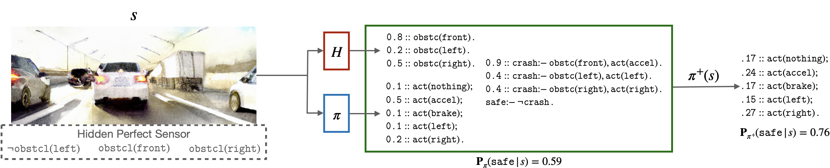
Figure 1: A motivation example of Probabilistic Logic Shields. We encode the interaction between the base policy $\pi$, the state-abstraction $H$ and the safety specification using a ProbLog program $\mathcal{T}$. This provides a uniform language to express many aspects of the shielding process. The shielded policy $\pi^{+}(s)$ decreases the probability of unsafe actions, e.g. acceleration and increases the likelihood of being safe.

2 Preliminaries

Probabilistic Logic Programming

We will introduce probabilistic logic programming (PLP) using the syntax of the ProbLog system De Raedt and Kimmig (2015). An atom is a predicate symbol followed by a tuple of logical variables and/or constants. A literal is an atom or its negation. A ProbLog theory (or program) $\mathcal{T}$ consists of a finite set of probabilistic facts $\mathcal{F}$ and a finite set of clauses $\mathcal{BK}$. A probabilistic fact is an expression of the form $\mathtt{p_{i}::f_{i}}$ where $\mathtt{p_{i}}$ denotes the probability of the fact $\mathtt{f_{i}}$ being true. It is assumed that the probabilistic facts are independent of one other (akin to the nodes with parents in Bayesian networks) and the dependencies are specified by clauses (or rules). For instance, $\mathtt{0.8::obstc(front).}$ states that the probability of having an obstacle in front is 0.8. A clause is a universally quantified expression of the form $\mathtt{h:\!\!-b_{1},...,b_{n}}$ where $\mathtt{h}$ is a literal and $\mathtt{b_{1},...,b_{n}}$ is a conjunction of literals, stating that $\mathtt{h}$ is true if all $\mathtt{b_{i}}$ are true. The clause defining $\mathtt{safe}$ in Fig. 1 states that it is safe when there is no crash. Each truth value assignment of all probabilistic facts $\mathcal{F}$, denoted by $\mathcal{F}_{k}$, induces a possible world $w_{k}$ where all ground facts in $w_{k}$ are true and all that are not in $w_{k}$ are false. Formally, the probability of a possible world $w_{k}$ is defined as follows.

$$P(w_{k})=\prod_{\mathtt{f_{i}}\in w_{k}}\mathtt{p_{i}}\prod_{\mathtt{f_{i}}\not\in w_{k}}\mathtt{(1-p_{i})}.$$ (1)

ProbLog allows for annotated disjunctions (ADs). An AD is a clause with multiple heads $\mathtt{h_{i}}$ that are mutually exclusive to one another, meaning that exactly one head is true when the body is true, and the choice of the head is governed by a probability distribution. An AD has the form of $\mathtt{p_{1}::h_{1};\cdots;p_{m}::h_{m}}$ where each $\mathtt{h_{i}}$ is the head of a clause and $\sum^{m}_{i=1}\mathtt{p_{i}}\leq 1$ De Raedt and Kimmig (2015); Fierens et al. (2015). For instance, $\{\mathtt{0.1::act(nothing);}$ $\mathtt{0.5::act(accel);}$ $\mathtt{0.1::act(brake);}$ $\mathtt{0.1::act(left);}$ $\mathtt{0.2::act(right)}\}$ is an AD (with no conditions), stating the probability with which each action will be taken. The success probability of an atom $q$ given a theory $\mathcal{T}$ is the sum of the probabilities of the possible worlds that entail $q$. Formally, it is defined as $P(q):=\sum_{w_{k}\models q}P(w_{k}).$ Given a set of atoms $E$ as evidence, the conditional probability of a query $q$ is $\mathbf{P}(q|E)=\frac{P(q,E)}{P(E)}$. For instance, in Fig. 1, the probability of being safe in the next state given that the agent accelerates is $\mathbf{P}(\mathtt{safe|act(accel)})=\frac{0.14}{0.5}=0.28$.

MDP

A Markov decision process (MDP) is a tuple $M=\langle S,A,T,R,\gamma\rangle$ where $S$ and $A$ are state and action spaces, respectively. $T(s,a,s^{\prime})=P(s^{\prime}|s,a)$ defines the probability of being in $s^{\prime}$ after executing $a$ in $s$. $R(s,a,s^{\prime})$ defines the immediate reward of executing $a$ in $s$ resulting in $s^{\prime}$. $\gamma\in[0,1]$ is the discount factor. A policy $\pi:S\times A\to[0,1]$ defines the probability of taking an action in a state. We use $\pi(a|s)$ to denote the probability of action $a$ in state $s$ under policy $\pi$ and $\pi(s)$ for the probability distribution over all the actions in state $s$.

Shielding

A shield is a reactive system that guarantees safety of the learning agent by preventing it from selecting any unsafe action at run time Jansen et al. (2020). Usually, a shield is provided as a Markov model and a temporal logical formula, jointly defining a safety specification. The shield constrains the agent’s exploration by only allowing it to take actions that satisfy the given safety specification. For example, when there is a car driving in front and the agent proposes to accelerate, a standard shield (Fig. 2, left) will reject the action as the agent may crash.

Policy Gradients

The objective of a RL agent is to find a policy $\pi_{\theta}$ (parameterized by $\theta$) that maximizes the total expected return along the trajectory, formally,

$$J(\theta)=\mathbb{E}_{\pi_{\theta}}[\sum_{t=0}^{\infty}\gamma^{t}r_{t}]$$

$J(\theta)$ is assumed to be finite for all policies. An important class of RL algorithms, particularly relevant in the setting of shielding, is based on policy gradients, which maximize $J(\theta)$ by repeatedly estimating the gradient $\nabla_{\theta}J(\theta)$. The general form of policy gradient methods is:

$$\nabla_{\theta}J(\theta)=\mathbb{E}_{\pi_{\theta}}[\sum_{t=0}^{\infty}\Psi_{t}\nabla_{\theta}\log\pi_{\theta}(s_{t},a_{t})]$$ (2)

where $\Psi_{t}$ is an empirical expectation of the return Schulman et al. (2018). The expected value is usually computed using Monte Carlo methods, requiring efficient sampling from $\pi_{\theta}$.

3 Probabilistic Logic Shields

3.1 Probabilistic Shielding

To reason about safety, we will assume that we have a safety-aware probabilistic model $\mathbf{P}(\mathtt{safe}|a,s)$, indicating the probability that an action $a$ is safe to execute in a state $s$. We use bold $\mathbf{P}$ to distinguish it from the underlying probability distributions $P(\cdot)$ of the MDP. Our safety-aware probabilistic model does not require that the underlying MDP is known. However, it needs to represent internally safe relevant-dynamics as the safety specification. Therefore, the safety-aware model $\mathbf{P}$ is not a full representation of the MDP, it is limited to safety-related properties.

Notice that for traditional logical shields actions are either safe or unsafe, which implies that $\mathbf{P}(\mathtt{safe}|a,s)=1$ or $0$. We are interested in the safety of policies, that is, in

$$\mathbf{P}_{\pi}(\mathtt{safe}|s)=\sum_{a\in A}\mathbf{P}(\mathtt{safe}|s,a)\pi(a|s).$$ (3)

By marginalizing out actions according to their probability under $\pi$, the probability $\mathbf{P}_{\pi}$ measures how likely it is to take a safe action in $s$ according to $\pi$.

Definition 3.1.

Probabilistic Shielding Given a base policy $\pi$ and a probabilistic safety model $\mathbf{P}(\mathtt{safe}|s,a)$, the shielded policy is

$$\pi^{+}(a|s) =\mathbf{P}_{\pi}(a|s,\mathtt{safe})=\frac{\mathbf{P}(\mathtt{safe}|s,a)}{\mathbf{P}_{\pi}(\mathtt{safe}|s)}\pi(a|s)$$ (4)

Intuitively, a shielded policy is a re-normalization of the base policy that increases (resp. decreases) the probabilities of the actions that are safer (resp. less safe) than average.

Proposition 1.

A shielded policy is always safer than its base policy in all states, i.e. $P_{\pi^{+}}(\mathtt{safe}|s)\geq P_{\pi}(\mathtt{safe}|s)$ for all $s$ and $\pi$. (A proof is in Appendix B)

3.2 Shielding with Probabilistic Logics

In this paper, we focus on probabilistic shields implemented through probabilistic logic programs. The ProbLog program defining probabilistic safety consists of three parts.

First, an annotated disjunction $\mathbf{\Pi}_{s}$, which represents the policy $\pi(a|s)$ in the logic program. For example, in Fig. 1, the policy $\pi(a|s)$ is represented as the annotated disjunction $\mathbf{\Pi}_{s}$ $=\{\mathtt{0.1::act(nothing);}$ $\mathtt{0.5::act(accel);}$ $\mathtt{0.1::act(brake);}$ $\mathtt{0.1::act(left);}$ $\mathtt{0.2::act(right)}\}$.

The second component of the program is a set of probabilistic facts $\mathbf{H}_{s}$ representing an abstraction of the current state. Such abstraction should contain information needed to reason about the safety of actions in that state. Therefore, it should not be a fair representation of the entire state $s$. For example, in Fig. 1, the abstraction is represented as the set of probabilistic facts: $\mathbf{H}_{s}=\{$ $\mathtt{0.8::obstc(front).}$ $\mathtt{0.2::obstc(left).}$ $\mathtt{0.5::obstc(right)}.\}$

The third component of the program is a safety specification $\mathcal{BK}$, which is a set of clauses and ADs representing knowledge about safety. In our example, the predicates $\mathtt{crash}$ and $\mathtt{safe}$ are defined using clauses. The first clause for $\mathtt{crash}$ states that the probability of having a crash is 0.9 if the agent accelerates when there is an obstacle in front of it. The clause for $\mathtt{safe}$ states that it is safe if no crash occurs.

Therefore, we obtain a ProbLog program $\mathcal{T}(s)=\mathcal{BK}\cup\mathbf{H}_{s}\cup\boldsymbol{\Pi}_{s}$, inducing a probabilistic measure $\textbf{P}_{\mathcal{T}}$. By querying this program, we can reason about safety of policies and actions. More specifically, we can use $\mathcal{T}(s)$ to obtain:

• action safety in $s$: $\textbf{P}(\mathtt{safe}|s,a)=\mathbf{P}_{\mathcal{T}}(\mathtt{safe}|a)$

• policy safety in $s$: $\textbf{P}_{\pi}(\mathtt{safe}|s)=\mathbf{P}_{\mathcal{T}}(\mathtt{safe})$

• the shielded policy in $s$: $\textbf{P}_{\pi}(a|s,\mathtt{safe})=\mathbf{P}_{\mathcal{T}}(a|\mathtt{safe})$

Notice that these three distributions can be obtained by querying the same identical program ProbLog program $\mathcal{T}$.

It is important to realize that although we are using the probabilistic logic programming language ProbLog to reason about safety, we could also have used alternative representations such as Bayesian networks, or other StarAI models De Raedt et al. (2016). The ProbLog representation is however convenient because it allows to easily model planning domains, it is Turing equivalent and it is differentiable. At the same time, it is important to note that the safety model in ProbLog is an abstraction, using possibly a different representation than that of the underlying MDP.

Perception Through Neural Predicates

The probabilities of both $\mathbf{\Pi}_{s}$ and $\mathbf{H}_{s}$ depend on the current state $s$. We compute these probabilities using two neural networks $\pi$ and $H$ operating on real valued inputs (i.e. images or sensors). We feed then the probabilities to the ProbLog program. As we depicted in Fig. 1, both these functions take a state representation $s$ as input (e.g. an image) and they output the probabilities the facts representing, respectively, the actions and the safe-relevant abstraction of the state. This feature is closely related to the notion of neural predicate, which can — for the purposes of this paper — be regarded as encapsulated neural networks inside logic. Since ProbLog programs are differentiable with respect to the probabilities in $\mathbf{\Pi}_{s}$ and $\mathbf{H}_{s}$, the gradients can be seamlessly backpropagated to network parameters during learning.

4 Probabilistic Logic Policy Gradient

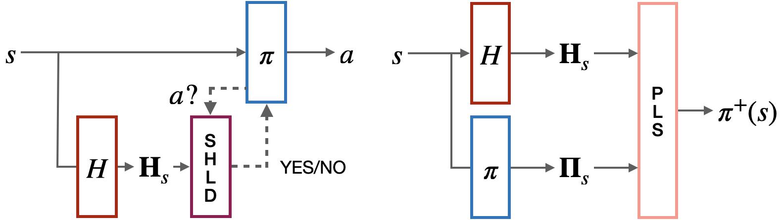
Figure 2: A comparison between a traditional rejection-based shield (SHLD) and a Probabilistic Logic Shield (PLS). Both shields take a policy $\pi$ and a set of noisy sensor readings $\mathbf{H_{s}}$ to compute a safe action. Left: The policy must keep sampling actions until a safe action is accepted by the rejection-based shield. This requires an assumption that an action is either completely safe or unsafe. Right: We replace SHLD with PLS that proposes a safer policy $\pi^{+}$ on the policy level without imposing the assumption.

In this section, we demonstrate how to use probabilistic logic shields with a deep reinforcement learning method. We will focus on real-vector states (such as images), but the safety constraint is specified symbolically and logically. Under this setting, our goal is to find an optimal policy in the safe policy space $\Pi_{\mathtt{safe}}=\{\pi\in\Pi|\mathbf{P}_{\pi}(\mathtt{safe}|s)=1,\forall s\in S\}$. Notice that it is possible that no optimal policies exist in the safe policy space. In this case, our aim will be to find a policy that it as safe as possible.

We propose a new safe policy gradient technique, which we call Probabilistic Logic Policy Gradient (PLPG). PLPG applies probabilistic logic shields and is guaranteed to converge to a safe and optimal policy if it exists.

4.1 PLPG for Probabilistic Shielding

To integrate PLS with policy gradient, we simply replace the base policy in Eq. 2 with the shielded policy obtained through Eq. 4. We call this a shielded policy gradient.

$$\mathbb{E}_{\pi^{+}_{\theta}}[ \sum_{t=0}^{\infty}\Psi_{t}\nabla_{\theta}\log\pi^{+}_{\theta}(a_{t}|s_{t})]$$ (5)

This requires the shield to be differentiable and cannot be done using rejection-based shields. The gradient encourages policies $\pi^{+}$ that are more rewarding, i.e. that has a large $\Psi$, in the same way of a standard policy gradient. It does so by assuming that unsafe actions have been filtered by the shield. However, when the safety definition is uncertain, unsafe actions may still be taken and such a gradient may still end up encouraging unsafe but rewarding policies.

For this reason, we introduce a safety loss to penalize unsafe policies. Intuitively, a safe policy should have a small safety loss, and the loss of a completely safe policy should be zero. The loss can be expressed by interpreting the policy safety as the probability that $\pi^{+}$ satisfies the safety constraint (using the semantic loss of Xu et al. (2018)); more formally, $L^{s}:=-\log\mathbf{P}_{\pi^{+}}(\mathtt{safe}|s)$. Then, the corresponding safety gradient is as follows.

$$-\mathbb{E}_{\pi^{+}_{\theta}}[\nabla_{\theta}\log\mathbf{P}_{\pi^{+}}(\mathtt{safe}|s)]$$ (6)

Notice that the safety gradient is not a shielding mechanism but a regret due to its loss-based nature. By combining the shielded policy gradient and the safety gradient, we obtain a new Safe RL technique.

Definition 4.1.

(PLPG) The probabilistic logic policy gradient $\nabla_{\theta}J(\theta)$ is

$$\mathbb{E}_{\pi^{+}_{\theta}}[ \sum_{t=0}^{\infty}\Psi_{t}\nabla_{\theta}\log\pi^{+}_{\theta}(a_{t}|s_{t})-\alpha\nabla_{\theta}\log\mathbf{P}_{\pi^{+}_{\theta}}(\mathtt{safe}|s_{t})]$$ (7)

where $\alpha$ is the safety coefficient that indicates the weight of the safety gradient.

We introduce the safety coefficient $\alpha$, a hyperparameter that controls the combination of the two gradients.

Both gradients in PLPG are essential. The shielded policy gradient forbids the agent from immediate danger and the safety gradient penalizes unsafe behavior. The interaction between shielded and loss-based gradients is still a very new topic, nonetheless, recent advances in neuro-symbolic learning have shown that both are important Ahmed et al. (2022). Our experiments shows that having only one but not both is practically insufficient.

4.2 Probabilistic vs Rejection-based Shielding

The problem of finding a policy in the safe policy space cannot be solved by rejection-based shielding (cf. Fig. 2, left) without strong assumptions, such as that a state-action pair is either completely safe or unsafe. It is in fact often assumed that a set of safe state-action pairs $SA_{\mathtt{safe}}$ is given. To implement a rejection-based shield, the agent must keep sampling from the base policy until an action $a$ is accepted. This approach implicitly conditions through very inefficient rejection sampling schemes as below, which has an unclear link to probabilistic semantics Robert et al. (1999).

$$\pi^{+}(a|s)=\frac{\mathbbm{1}_{[(s,a)\in SA_{\mathtt{safe}}]}\pi(a|s)}{\sum\limits_{a^{\prime}\in A}\mathbbm{1}_{[(s,a^{\prime})\in SA_{\mathtt{safe}}]}\pi(a^{\prime}|s)}$$ (8)

Convergence Under Perfect Safety Information

It is common for existing shielding approaches to integrate policy gradients with a rejection-based shield, e.g. Eq. 8, resulting in the following policy gradient.

$$\nabla_{\theta}J(\theta)=\mathbb{E}_{\pi^{+}_{\theta}}[\sum_{t=0}^{\infty}\Psi_{t}\nabla_{\theta}\log\pi_{\theta}(s_{t},a_{t})]$$ (9)

It is a known problem that this approach may result in sub-optimal policies, even though the agent has perfect safety information Kalweit et al. (2020); Ray et al. (2019); Hunt et al. (2021); Anderson et al. (2020). This is due to a policy mismatch between $\pi^{+}$ and $\pi$ in Eq. 9. More specifically, Eq. 9 is an off-policy algorithm, meaning that the policy used to explore (i.e. $\pi^{+}$) is different from the policy that is updated (i.e. $\pi$). For any off-policy policy gradient method to converge to an optimal policy (even in the tabular case), the behavior policy (to explore) and the target policy (to be updated) must appropriately visit the same state-action space, i.e., if $\pi(a|s)>0$ then $\pi^{+}(a|s)>0$ Sutton and Barto (2018). This requirement is violated by Eq. 9.

PLPG, on the other hand, reduces to Eq. 5 when given perfect sensor information of the state. Since it has the same form as the standard policy gradient (Eq. 9), PLPG is guaranteed to converge to an optimal policy according to the Policy Gradient Theorem Sutton et al. (2000).

Proposition 2.

PLPG, i.e. Eq. 7, converges to an optimal policy given perfect safety information in all states.

It should be noted that the base policy learnt by PLPG is unlikely to be equivalent to the policy that would have been learnt without a shield, all other things being equal. That is, in general, $\pi_{\theta}$ in Eq. 9 will not tend to be the same as $\pi_{\theta}$ in  Eq. 7 as learning continues. This is because the parameters $\theta$ in Eq. 7 depend on $\pi^{+}_{\theta}$ instead of $\pi_{\theta}$, and $\pi_{\theta}$ is learnt in a way to make $\pi^{+}$ optimal given safety imposed by the shield.

Learning From Unsafe Actions

PLPG has a significant advantage over a rejection-based shield by learning not only from the actions accepted by the shield but also from the ones that would have been rejected. This is a result of the use of ProbLog programs that computes the safety of all available actions in the current state, allowing us to update the base policy in terms of safety without having to actually execute the other actions.

Leveraging Probabilistic Logic Programming

Probabilistic logic programs can, just like Bayesian networks, be compiled into circuits using knowledge compilation Darwiche (2003). Although probabilistic inference is hard (#P-complete), once the circuit is obtained, inference is linear in the size of the circuit De Raedt and Kimmig (2015); Fierens et al. (2015). Furthermore, the circuits can be used to compute gradients and the safety model only needs to be compiled once. We show a compiled program in Appendix C. Our PLP language is still restricted to discrete actions, although it should be possible to model continuous actions using extensions thereof in future work Nitti et al. (2016).

5 Experiments

Now, we present an empirical evaluation of PLPG, when compared to other baselines in terms of return and safety.

Experimental Setup

Experiments are run in three environments. (1) Stars, the agent must collect as many stars as possible without going into a stationary fire; (2) Pacman, the agent must collect stars without getting caught by the fire ghosts that can move around, and (3) Car Racing, the agent must go around the track without driving into the grass area. We use two configurations for each domain. A detailed description is in Appendix A.

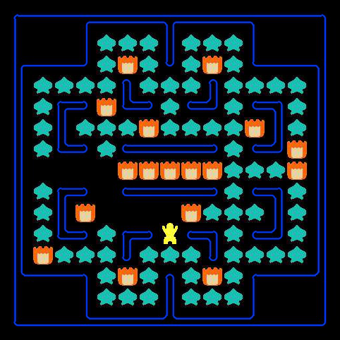
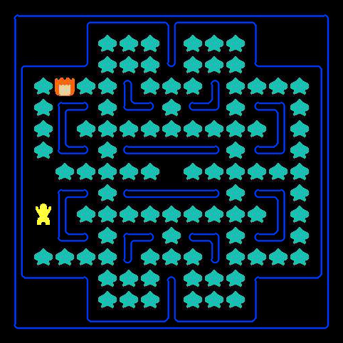
Figure 3: The domains of Stars, Pacman and Car Racing. The difference between Stars and Pacman is that fires in Stars are stable and the ones in Pacman move around.

We compare PLPG to three RL baselines.

• PPO, a standard safety-agnostic agent that starts with a random initial policy Schulman et al. (2017).

• VSRL, an agent augmented with a deterministic rejection-based shield Hunt et al. (2021). Its structure is shown in Fig. 2 (left).

• $\epsilon$-VSRL a new risk-taking variant of VSRL that has a small $\epsilon$ probability of accepting any action, akin to $\epsilon$-greedy Fernández and Veloso (2006) As $\epsilon$-VSRL simulates an artificial noise/distrust in the sensors, we expect that it improves VSRL’s ability to cope with noise.

In order to have a fair comparison, VSRL, $\epsilon$-VSRL and PLPG agents have identical safety sensors and safety constraints, and PPO does not have any safety sensors. We do not compare to shielding approaches that require a full model of the environment since they are not applicable here. We train all agents in all domains using 600k learning steps and all experiments are repeated using five different seeds.

In our experiments, we answer the following questions :

• Does PLPG produce safer and more rewarding policies than its competitors?

• What is the effect of the hyper-parameters $\alpha$ and $\epsilon$?

• Does the shielded policy gradient or the safety gradient have more impact on safety in PLPG?

• What are the performance and the computational cost of a multi-step safety look-ahead PLS?

Metrics

We compare all agents in terms of two metrics: (1) average normalized return, i.e. the standard per-episode normalized return averaged over the last 100 episodes; (2) cumulative normalized violation, i.e. the accumulated number of constraint violations from the start of learning. The absolute numbers are listed in Appendix D.

Probabilistic Safety via Noisy Sensor Values

We consider a set of noisy sensors around the agent for safety purposes. For instance, the four fire sensor readings in Fig. 3 (left) might $\{\mathtt{0.6::fire(0,1).}$ $\mathtt{0.1::fire(0,-1).}$ $\mathtt{0.1::fire(-1,0).}$ $\mathtt{0.4::fire(1,0).}\}$ These sensors provide to the shield only local information of the learning agent. PLPG agents are able to directly use the noisy sensor values. However, as VSRL and $\epsilon$-VSRL agents require 0/1 sensor values to apply formal verification, noisy sensor readings must be discretized to $\{0,1\}$. For example, the above fire sensor readings become $\{\mathtt{1::fire(0,1).}$ $\mathtt{0::fire(0,-1).}$ $\mathtt{0::fire(-1,0).}$ $\mathtt{0::fire(1,0).}\}$ For all domains, the noisy sensors are standard, pre-trained neural approximators of an accuracy higher than $99\%$. The training details are presented in Appendix A. Even with such accurate sensors, we will show that discretizing the sensor values, as in VSRL, is harmful for safety. Details of the pre-training procedure are in Appendix A.

Q1: Lower Violation and Higher Return

We evaluate how much safer and more rewarding PLPG is compared to baselines by measuring the cumulative safety violation and the average episodic return during the learning process. Before doing so, we must select appropriate hyperparameters for PLPG and VSRL agents. Since our goal is to find an optimal policy in the safe policy space, we select the $\alpha\in\{0,0.1,0.5,1,5\}$ and $\epsilon\in\{0,0.005,0.01,0.05,0.1,0.2,0.5,1.0\}$ values that result in the lowest violation in each domain. The hyperparameter choices are listed in Appendix D. These values are fixed for the rest of the experiments (except for Q2 where we explicitly analyze their effects). We show that PLPG achieves the lowest violation while having a comparable return to other agents.

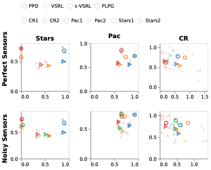
Figure 4: Trade-off between Violation (x-axis) and Return (y-axis). Each small data point is an agent’s policy and the large data points are the average of five seeds. An ideal policy should lie in the upper-left corner.

The results are plotted in Fig. 4 where each data point is a policy trained for 600k steps. Fig. 4 clearly shows that PLPG is the safest in most tested domains. When augmented with perfect sensors, PLPG’s violation is lower than PPO by 50.2% and lower than VSRL by 25.7%. When augmented with noisy sensors, PLPG’s violation is lower than PPO by 51.3%, lower than VSRL by 24.5% and lower than $\epsilon$-VSRL by 13.5%. Fig. 4 also illustrates that PLPG achieves a comparable (or slightly higher) return while having the lowest violation. When augmented with perfect sensors, PLPG’s return is higher than PPO by 0.5% and higher than VSRL by 4.8%. When augmented with noisy sensors, PLPG’s return is higher than PPO by 4.5%, higher than VSRL by 6.5% and higher than $\epsilon$-VSRL by 6.7%.

Car Racing has complex and continuous action effects compared to the other domains. In CR, safety sensor readings alone are not sufficient for the car to avoid driving into the grass as they do not capture the inertia of the car, which involves the velocity and the underlying physical mechanism such as friction. In domains where safety sensors are not sufficient, the agent must be able to act a little unsafe to learn, as PPO, $\epsilon$-VSRL and PLPG can do, instead of completely relying on sensors such as VSRL. Hence, compared to the safety-agnostic baseline PPO, while $\epsilon$-VSRL and PLPG respectively reduce violations by 37.8% and 50.2%, VSRL causes 18% more violations even when given perfect safety sensors. Note that we measure the actual violations instead of policy safety $P_{\pi}(\mathtt{safe}|s)$. The policy safety during the learning process is plotted in Appendix D.

Q2: Selection of Hyperparameters $\alpha$ and $\epsilon$

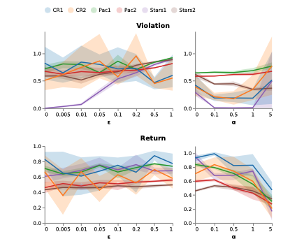
Figure 5: The episodic return and cumulative constraint violation of VSRL (left) and PLPG (right) agents in noisy environments. Left: The effect of $\epsilon$ is not significant. Right: Increasing $\alpha$ gives a convex trend in both return and violation. The absolute numbers are listed in Appendix D.

We analyze how the hyper-parameters $\alpha$ and $\epsilon$ respectively affect the performance of PLPG and VSRL in noisy environments. Specifically, we measure the episodic return and cumulative constraint violation. The results are plotted in Fig. 5.

The effect of different values of $\alpha$ to PLPG agents is clear. Increasing $\alpha$ gives a convex trend in both the return and the violation counts. The optimal value of $\alpha$ is generally between $0.1$ and $1$, where the cumulative constraint violation and the return are optimal. This illustrates the benefit of combining the shielded policy gradient and the safety gradient. On the contrary, the effect of $\epsilon$ to VSRL agents is not significant. Increasing $\epsilon$ generally improves return but worsens constraint violation. This illustrates that simply randomizing the policy is not effective in improving the ability of handling noisy environments. Notice that there is no one-to-one mapping between the two hyper-parameters, as $\alpha$ controls the combination of the gradients and $\epsilon$ controls the degree of unsafe exploration.

Q3: PLPG Gradient Analysis

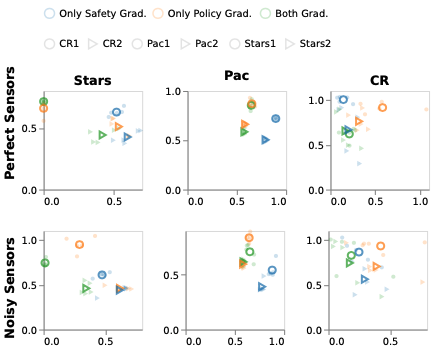
Figure 6: Trade-off between Violation (x-axis) and Return (y-axis). Each data point is an agent’s policy and the big data points are the average of five seeds.

We analyze how the shielded policy gradient and the safety gradient interact with one another. To do this, we introduce two ablated agents, one uses only safety gradients (Eq. 5) and the other uses only policy gradients (Eq. 6). The results are plotted in Fig. 6 where each data point is a policy trained for 600k steps.

Fig. 6 illustrates that combining both gradients is safer than using only one gradient. When augmented with perfect sensors, the use of both gradients has a violation that is lower than using only safety or policy gradient by 24.7% and 10.8%, respectively. When augmented with noisy sensors, using both gradients has a violation that is lower than using only safety or policy gradient by 25.5% and 15.5%, respectively. Nonetheless, the importance of policy and safety gradients varies among domains. In Stars and Pacman, using only policy gradients causes fewer violations than using only safety gradients. In CR, however, using only safety gradients causes fewer violations. This is a consequence of the inertia of the car not being fully captured by safety sensors, as discussed in Q1.

Q4: Multi-step Safety Look-ahead

We analyze the behaviour of PLPG when we use probabilistic logic shields for multi-step safety look-ahead. In this case, the safety program requires more sensors around the agent for potential danger over a larger horizon in the future. In Pacman, for example, new sensors are required to detect whether there is a ghost N units away where N is the safety horizon. We analyze the behavior/performance in terms of return/violation and computational cost. The results are shown in Table 1. Increasing the horizon causes an exponential growth in the compiled circuit size and the corresponding inference time. However, we can considerably improve both safety and return, especially when moving from one to two steps.

Safety horizon	1 step	2 steps	3 steps	4 steps
#sensors	4	12	24	40
Circuit size	116	1073	8246	373676
Compilation (s)	0.29	0.70	1.70	15.94
Evaluation (s)	0.01	0.08	0.66	27.39
Ret./Vio.	0.81 / 0.82	0.85 / 0.65	0.86 / 0.57	-

Table 1: Multi-step Safety Look-ahead

6 Related Work

Safe RL.

Safe RL aims to avoid unsafe consequences through the use of various safety representations  García and Fernández (2015). There are several ways to achieve this goal. One could constrain the expected cost Achiam et al. (2017); Moldovan and Abbeel (2012), maximize safety constraint satisfiability through a loss function Xu et al. (2018), add a penalty to the agent when the constraint is violated Pham et al. (2018); Tessler et al. (2019); Memarian et al. (2021), or construct a more complex reward structure using temporal logic De Giacomo et al. (2021); Camacho et al. (2019); Jiang et al. (2021); Hasanbeig et al. (2019); Den Hengst et al. (2022). These approaches express safety as a loss, while our method directly prevents the agent from taking actions that can potentially lead to safety violation.

Probabilistic Shields.

Shielding is a safe reinforcement learning approach that aims to completely avoid unsafe actions during the learning process Alshiekh et al. (2018); Jansen et al. (2020). Previous shielding approaches have been limited to symbolic state spaces and are not suitable for noisy environments Jansen et al. (2020); Harris and Schaub (2020); Hunt et al. (2021); Anderson et al. (2020). To address uncertainty, some methods incorporate randomization, e.g. simulating future states in an emulator to estimate risk Li and Bastani (2020); Giacobbe et al. (2021), using $\epsilon$-greedy exploration that permits unsafe actions García and Fernández (2019), or randomizing the policy based on the current belief state Karkus et al. (2017). To integrate shielding with neural policies, one can translate a neural policy to a symbolic one that can be formally verified Bastani et al. (2018); Verma et al. (2019). However, these methods rely on sampling and do not have a clear connection to uncertainty present in the environment while our method directly exploits such uncertainty through the use of PLP principles. Belief states can capture uncertainty but require an environment model to to keep track of the agent’s belief state, which is a stronger assumption than our method Junges et al. (2021); Carr et al. (2022).

Differentiable layers for neural policies.

The use of differentiable shields has gain some attention in the field. One popular approach is to add a differentiable layer to the policy network to prevent constraint violations. Most of these methods focus on smooth physical rules Dalal et al. (2018); Pham et al. (2018); Cheng et al. (2019) and only a few involve logical constraints. In Kimura et al. (2021), an optimization layer is used to transform a state-value function into a policy encoded as a logical neural network. Ahmed et al. (2022) encode differentiable and hard logical constraints for neural networks using PLP. While being similar, this last model focuses on prediction tasks and do not consider a trade-off between return and constraint satisfiability.

7 Conclusion

We introduced Probabilistic Logic Shields, a proof of concept of a novel class of end-to-end differentiable shielding techniques. PLPG enable efficient training of safe-by-construction neural policies. This is done by using a probabilistic logic programming layer on top of the standard neural policy. PLPG is a generalization of classical shielding Hunt et al. (2021) that allows for both deterministic and probabilistic safety specifications. Future work will be dedicated to extending PLS to be used with a larger class of RL algorithms such as the ones with continuous policies.

Appendix A Experiment settings

Experiments are run on machines that consist of Intel(R) Xeon(R) E3-1225 CPU cores and 32Gb memory. All environments in this work are available on GitHub under the MIT license. The measurements are obtained by taking the average of five seeds. All agents are trained using PPO in stable-baselines Hill et al. [2018] with batch size=512, n_epochs=15, n_steps=2048, clip range=0.1, learning rate=0.0001. All policy networks and value networks have two hidden layers of size 64. All the other hyperparameters are set to default as in stable-baselines Hill et al. [2018]. The source code will be available upon publication of the paper.

A.1 Stars

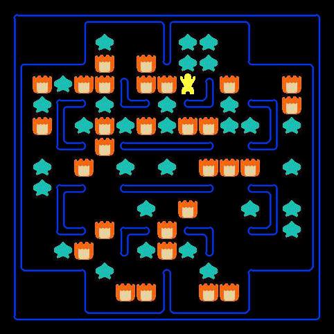
Figure 7: Left: A Stars image. Middle: A Stars state (downsampled from the left). Right: A example to pre-train noisy sensors.

We build the Stars environments using Berkeley’s Pac-Man Project . Our environment is a 15 by 15 grid world containing stars and fires, e.g. Fig. 7, where the agent can move around using five discrete, deterministic actions: stay, up, down, left, right. Each action costs a negative reward of $-0.1$. The task of the agent is to collect all stars in the environment. Collecting one star yields a reward of $1$. When the agent finds all stars, the episode ends with a reward of $10$. If the agent crashes into fire or has taken $200$ steps (maximum episode length), the episode ends with no rewards. Each state is a downsampled, grayscale image where each pixel is a value between -1 and 1, e.g. Fig. 7 (right).

We use the following probabilistic logic shield. The $\mathtt{act/1}$ predicates represent the base policy and the $\mathtt{fire/2}$ predicates represent whether there is fire in an immediate neighboring grid. These predicates are neural predicates, meaning that all probabilities $\mathtt{a_{i}}$ (resp. $\mathtt{f_{i}}$ will be substituted by real values in $[0,1]$, produced by the underlying base policy (resp. perfect or noisy sensors). In Fig. 7 (right), the sensors may produce $\{\mathtt{0::fire(0,1)}$, $\mathtt{0::fire(0,-1)}$, $\mathtt{1::fire(-1,0)}$, $\mathtt{0::fire(1,0)}\}$.

% BASE POLICY
a0::act(stay); a1::act(up);
a2::act(down); a3::act(left);
a4::act(right).

% SENSORS
f0::fire( 0, 1).  f1::fire( 0,-1).
f2::fire(-1, 0).  f3::fire( 1, 0).

% SAFETY LOOKAHEAD
xagent(stay, 0, 0).  xagent(left,-1, 0).
xagent(right,1, 0).  xagent(up,   0, 1).
xagent(down, 0,-1).

% SAFETY CONSTRAINT
crash:- act(A),
        xagent(A, X, Y), fire(X, Y).
safe:- not(crash).

A.2 Pacman

Pacman is more complicated than the Stars in that the fire ghosts can move around and their transition models are unknown. All the other environmental parameters are the same as Stars.

We use the following probabilistic logic shield to perform a two-step look-ahead. The agent has 12 sensors to detect whether there is a fire ghost one or two units away. The agent is assumed to follow the policy at $T=0$ and then do nothing at $T=1$. The fire ghosts are assumed to be able to move to any immediate neighboring cells at $T=0$ and $T=1$. A crash can occur at $T=0$ or $T=1$.

% BASE POLICY
a0::act(stay); a1::act(up);
a2::act(down); a3::act(left);
a4::act(right).

% SENSORS
f0:: fire(0, 0, 1). f1:: fire(0, 0,-1).
f2:: fire(0,-1, 0). f3:: fire(0, 1, 0).
f4:: fire(0, 0, 2). f5:: fire(0, 0,-2).
f6:: fire(0,-2, 0). f7:: fire(0, 2, 0).
f8:: fire(0, 1, 1). f9:: fire(0, 1,-1).
f10::fire(0,-1, 1). f11::fire(0,-1,-1).

% SAFETY LOOKAHEAD
fire(T, X, Y):-
    fire(T-1, PrevX, PrevY),
    move(PrevX, PrevY, _, X, Y).

agent(1, X, Y):-
    action(A), move(0, 0, A, X, Y).

agent(2, X, Y):- agent(1, X, Y).

move(X, Y, stay,  X,   Y).
move(X, Y, left,  X-1, Y).
move(X, Y, right, X+1, Y).
move(X, Y, up,    X,   Y+1).
move(X, Y, down,  X,   Y-1).

% SAFETY CONSTRAINT
crash:- fire(T, X, Y), agent(T, X, Y).
safe:- not(crash).

A.3 Car Racing

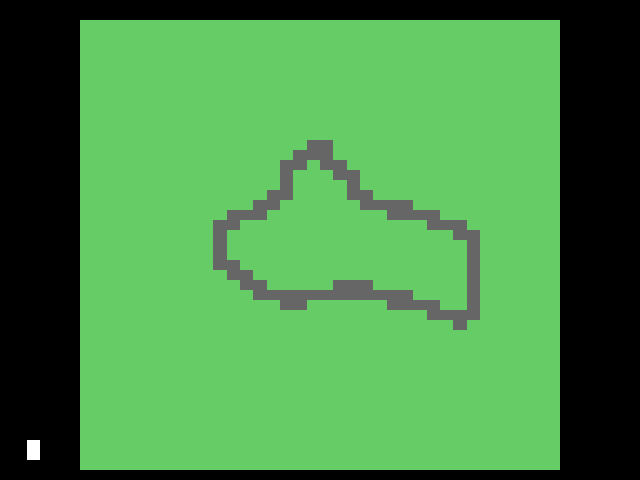
Figure 8: Left: A lap in Car Racing (Configuration 1). Middle: A CR image. We mark the sensors around the agent white but they not visible in training. Right: A CR state (downsampled from the middle).

We simplify Gym’s Car Racing environment Brockman et al. [2016]. Our environment is a randomly generated car track, e.g. Fig. 8 (left). At the beginning, the agent will be put on the track, e.g. Fig. 8 (middle). The task of the agent is to drive around the track (i.e. to finish one lap) within 1000 frames. In each frame, the agent takes a discrete action: do-nothing, accelerate, brake, turn-left or turn-right. Each action costs a negative reward of $-0.1$. The agent gets a small reward if it continues to follow the track. The agent does not get a penalty for driving on the grass, however, if the car drives outside of the map (i.e. the black part in Fig. 8, left), the episode ends with a negative reward of $-100$. Each state is a downsampled, grayscale image where each pixel is a value between $-1$ and $1$, e.g. Fig. 8 (right).

The original environment has a continuous action space that consists of three parameters: steering, gas and break with the minimum values $[-1,0,0]$ and the maximum values $[+1,+1,+1]$. In this paper, all agents use five discrete actions: do-nothing ($[0,0,0]$), accelerate ($[0,1,0]$), brake ($[0,0,0.8]$), turn-left ($[-1,0,0]$), turn-right ($[1,0,0]$).

We use the following probabilistic logic shield. The $\mathtt{act/1}$ predicates represent the base policy and the $\mathtt{grass/1}$ predicates represent whether there is grass in front, on the left or right hand side of the agent. In Fig. 8 (middle), the sensors may produce $\{\mathtt{0::grass(0)}$, $\mathtt{0::grass(1)}$ $\mathtt{0::grass(2)}\}$.

% BASE POLICY
a0::act(dn);   a1::act(accel);
a2::act(brake);
a3::act(left); a4::act(right).

% SENSORS
g0::grass(front).  g1::grass(left).
g2::grass(right).

% SAFETY LOOKAHEAD
ingrass:-
    grass(left), not(grass(right)),
    (act(left); act(accel)).
ingrass:-
    not(grass(left)), grass(right),
    (act(right); act(accel)).

% SAFETY CONSTRAINT
safe:- not(ingrass).

A.4 Approximating Noisy Sensors

We approximate noisy sensors using convolutional neural networks. In all the environments, we use 4 convolutional layers with respectively 8,16,32,64 (5x5) filters and relu activations. The output is computed by a dense layer with sigmoid activation function. The number of output neurons depends on the ProbLog program for that experiment (see Appendix A.1). We pre-train the networks and then we fix them during the reinforcement learning process. The pre-training strategy is the following. We generated randomly 3k images for Stars and Pacman with 30 fires and 30 stars, e.g. Fig. 7 (right), and 2k images for Car Racing, e.g. Fig. 8 (right). We selected the size of the pre-training datasets in order to achieve an accuracy higher than 99% on a validation set of 100 examples.

Appendix B Safety Guarantees of Probabilistic Logic Shield

In Definition 3.1, a shielded policy $\pi^{+}$ is always safer than its base policy $\pi$ for all $s$ and $\pi$, i.e.

$$\mathbf{P}_{\pi^{+}}(\mathtt{safe}|s)\geq\mathbf{P}_{\pi}(\mathtt{safe}|s)\mbox{ }\forall\pi\in\Pi\mbox{ and }\forall s\in S$$

Proof.

$$\mathbf{P}_{\pi^{+}}(\mathtt{safe}|s) \triangleright$$ Eq. 3

$$= \sum_{a\in A}\pi^{+}(a|s)\mathbf{P}(\mathtt{safe}|s,a) \triangleright$$ Eq. 4

$$= \frac{1}{\mathbf{P}_{\pi}(\mathtt{safe}|s)}[\sum_{a\in A}\pi(a|s)\mathbf{P}(\mathtt{safe}|s,a)^{2}] \triangleright$$ Jensen’s inequality

$$\geq \frac{1}{\mathbf{P}_{\pi}(\mathtt{safe}|s)}[\sum_{a\in A}\pi(a|s)\mathbf{P}(\mathtt{safe}|s,a)]^{2} \triangleright$$ Eq. 3

$$= \mathbf{P}_{\pi}(\mathtt{safe}|s)$$

The inequality comes from Jensen’s inequality Pishro-Nik [2014], which states that $\mathbb{E}[g(X)]\geq g(\mathbb{E}[X])$ for any convex function $g(X)$. In this proof, $g(X)=X^{2}$. ∎

Appendix C A Compiled Circuit

The following program is compiled to the circuit in Fig. 9.

0.2::act(dn); 0.6::act(left);
0.2::act(right).
0.8::ghost(left).  0.1::ghost(right).
crash:- act(left), ghost(left).
crash:- act(right), ghost(right).

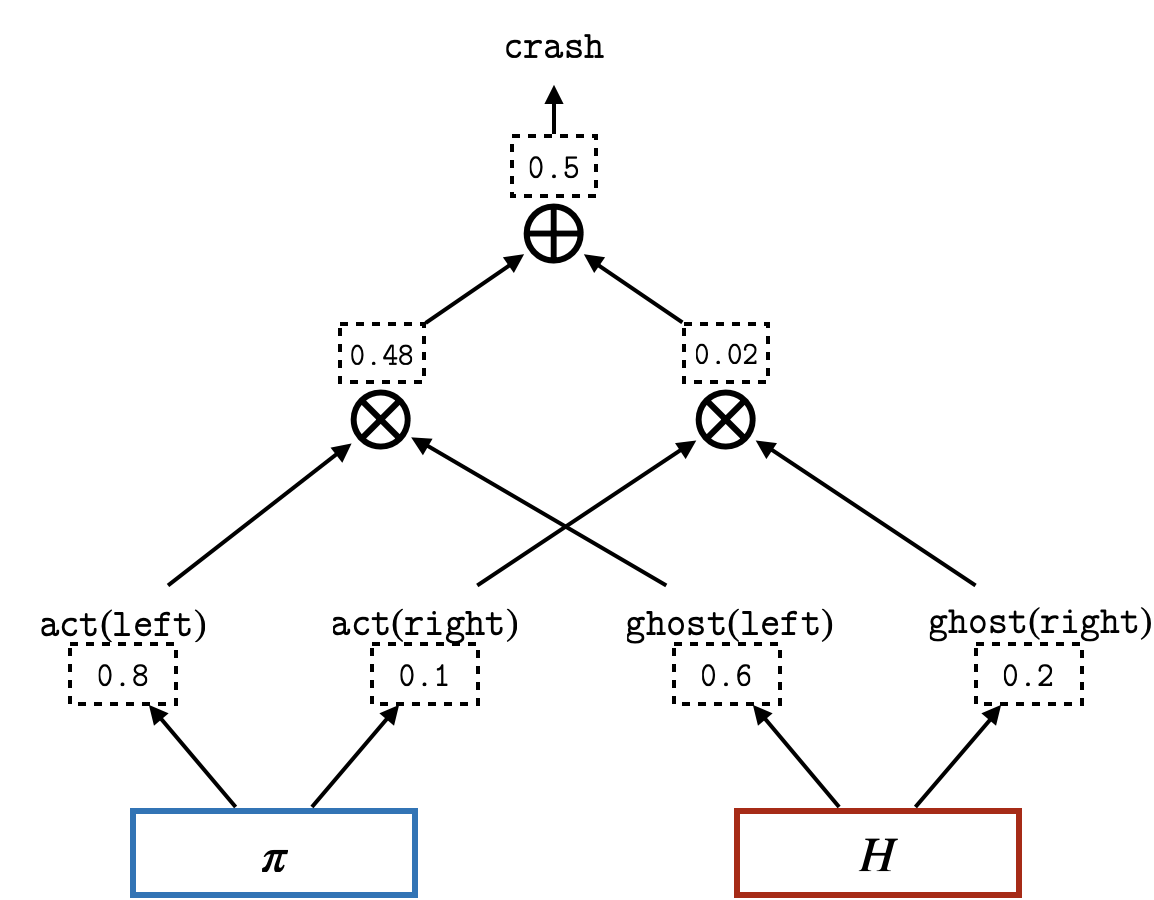
Figure 9: A circuit compiled from a program.

	Description	Return Range	Violation Range	Perfect Sensors	Noisy Sensors
				$\alpha$	$\epsilon$	$\alpha$
Stars1	Deterministic actions	[0, 45]	[0, 15k]	0.5	0.005	1
Stars2	Stochastic actions			1	0.01	1
Pacman1	One ghost	[0, 40]	[0, 7k]	0.1	0.05	0.5
Pacman2	Two ghosts		[0, 15k]	0.5	0.005	0.1
Car Racing1	Smoother track	[0, 900]	[0, 1]	0.5	0.5	1
Car Racing2	Curlier track			0.1	0.5	0.5

Table 2: Summary of configurations.

Appendix D Experiment Details

We run two configurations for each domain. The second configuration is more challenging than the first one. The configurations may have different normalization ranges and hyperparameters. We select the hyperparameters that result in the lowest violations in each configuration. Table 2 lists a summary of all configurations and all other tables follows this table if not explicitly specified.

We train all agents in all configurations using 600k learning steps and all experiments are repeated using five different seeds. The following tables list the normalized, average return and violation values of the five runs. Table 3 lists the return/violation results of all agents (cf. the large data points in Fig. 4). Table 4 lists the return/violation results for PLPG gradient analysis (cf. the large data points in Fig. 6). Tables 5 and 6 respectively list the return/violation results for $\alpha\in\{0,0.1,0.5,1,5\}$ and $\epsilon\in\{0,0.005,0.01,0.05,0.1,0.2,0.5,1.0\}$ (cf. Fig. 5).

Return/Violation	No Safety	Perfect Sensors		Noisy Sensors
	PPO	VSRL	PLPG	VSRL	$\epsilon$-VSRL	PLPG
Stars1	0.68 / 0.90	0.57 / 0.00	0.71 / 0.00	0.61 / 0.00	0.64 / 0.03	0.74 / 0.01
Stars2	0.50 / 0.89	0.43 / 0.58	0.44 / 0.42	0.43 / 0.59	0.46 / 0.52	0.46 / 0.35
Pacman1	0.74 / 0.92	0.72 / 0.74	0.85 / 0.65	0.71 / 0.72	0.75 / 0.65	0.71 / 0.65
Pacman2	0.56 / 0.82	0.56 / 0.62	0.59 / 0.58	0.46 / 0.67	0.51 / 0.62	0.62 / 0.59
Car Racing1	0.77 / 0.60	0.74 / 0.84	0.62 / 0.21	0.83 / 0.82	0.88 / 0.47	0.83 / 0.18
Car Racing2	0.58 / 0.55	0.55 / 0.67	0.65 / 0.17	0.67 / 0.51	0.70 / 0.45	0.74 / 0.17

Table 3: Normalized return and violation for all agents (cf. the large data points in Fig. 4).

Return/Violation	Perfect Sensors			Noisy Sensors
	Only Safety Grad	Only Policy Grad	Both	Only Safety Grad	Only Policy Grad	Both
Stars1	0.63 / 0.52	0.66 / 0.00	0.71 / 0.00	0.61 / 0.47	0.95 / 0.29	0.74 / 0.01
Stars2	0.43 / 0.60	0.51 / 0.53	0.44 / 0.42	0.44 / 0.62	0.46 / 0.62	0.46 / 0.35
Pacman1	0.72 / 0.89	0.87 / 0.65	0.85 / 0.65	0.54 / 0.88	0.84 / 0.64	0.71 / 0.65
Pacman2	0.51 / 0.79	0.66 / 0.58	0.59 / 0.58	0.39 / 0.78	0.60 / 0.58	0.62 / 0.59
Car Racing1	1.00 / 0.14	0.91 / 0.58	0.62 / 0.21	0.86 / 0.25	0.93 / 0.42	0.83 / 0.18
Car Racing2	0.67 / 0.20	0.76 / 0.32	0.65 / 0.17	0.56 / 0.29	0.70 / 0.39	0.74 / 0.17

Table 4: Analysis of PLPG gradients (cf. the large data points in Fig. 6).

$\alpha$	0	0.1	0.5	1	5
Stars1	0.95 / 0.29	0.68 / 0.01	0.68 / 0.01	0.74 / 0.01	0.17 / 0.50
Stars2	0.46 / 0.62	0.53 / 0.44	0.51 / 0.45	0.46 / 0.35	0.34 / 0.37
Pacman1	0.84 / 0.64	0.79 / 0.66	0.71 / 0.65	0.56 / 0.69	0.31 / 0.77
Pacman2	0.60 / 0.58	0.62 / 0.59	0.50 / 0.62	0.43 / 0.62	0.27 / 0.67
Car Racing1	0.93 / 0.42	0.99 / 0.19	0.82 / 0.19	0.83 / 0.18	0.47 / 0.52
Car Racing2	0.70 / 0.39	0.84 / 0.21	0.74 / 0.17	0.60 / 0.34	0.21 / 0.77

Table 5: The return and violation of different $\alpha$ values in noisy environments (cf. Fig. 5).

$\epsilon$	0 (VSRL)	0.005	0.01	0.05	0.1	0.2	0.5	1 (PPO)
Stars1	0.61 / 0.00	0.64 / 0.03	0.69 / 0.07	0.76 / 0.30	0.69 / 0.54	0.76 / 0.65	0.68 / 0.80	0.68 / 0.90
Stars2	0.43 / 0.59	0.46 / 0.59	0.46 / 0.52	0.46 / 0.62	0.48 / 0.67	0.47 / 0.78	0.49 / 0.85	0.50 / 0.89
Pacman1	0.71 / 0.72	0.64 / 0.81	0.66 / 0.80	0.75 / 0.65	0.66 / 0.86	0.72 / 0.71	0.77 / 0.84	0.74 / 0.92
Pacman2	0.46 / 0.67	0.51 / 0.62	0.48 / 0.67	0.52 / 0.65	0.51 / 0.68	0.53 / 0.70	0.54 / 0.74	0.56 / 0.82
Car Racing1	0.83 / 0.82	0.65 / 0.65	0.61 / 0.84	0.67 / 0.80	0.75 / 0.72	0.66 / 0.73	0.88 / 0.47	0.77 / 0.60
Car Racing2	0.67 / 0.51	0.36 / 0.62	0.67 / 0.75	0.43 / 0.86	0.63 / 0.57	0.52 / 0.95	0.70 / 0.45	0.58 / 0.55

Table 6: The return and violation of different $\epsilon$ values in noisy environments (cf. Fig. 5).

We plot episodic return, cumulative violation and step-wise policy safety in the learning process for all agents ($\mathbf{P}_{\pi^{+}}(\mathtt{safe}|s)$ for shielded agents and $\mathbf{P}_{\pi}(\mathtt{safe}|s)$ for PPO). Fig. 11 plots these curves for the agents augmented with perfect sensors and Fig. 10 for the ones with noisy sensors. PPO agents are plotted in both figures as a baseline but they are not augmented with any sensors. The return and policy safety curves are smoothed by taking the exponential moving average with the coefficient of 0.05.

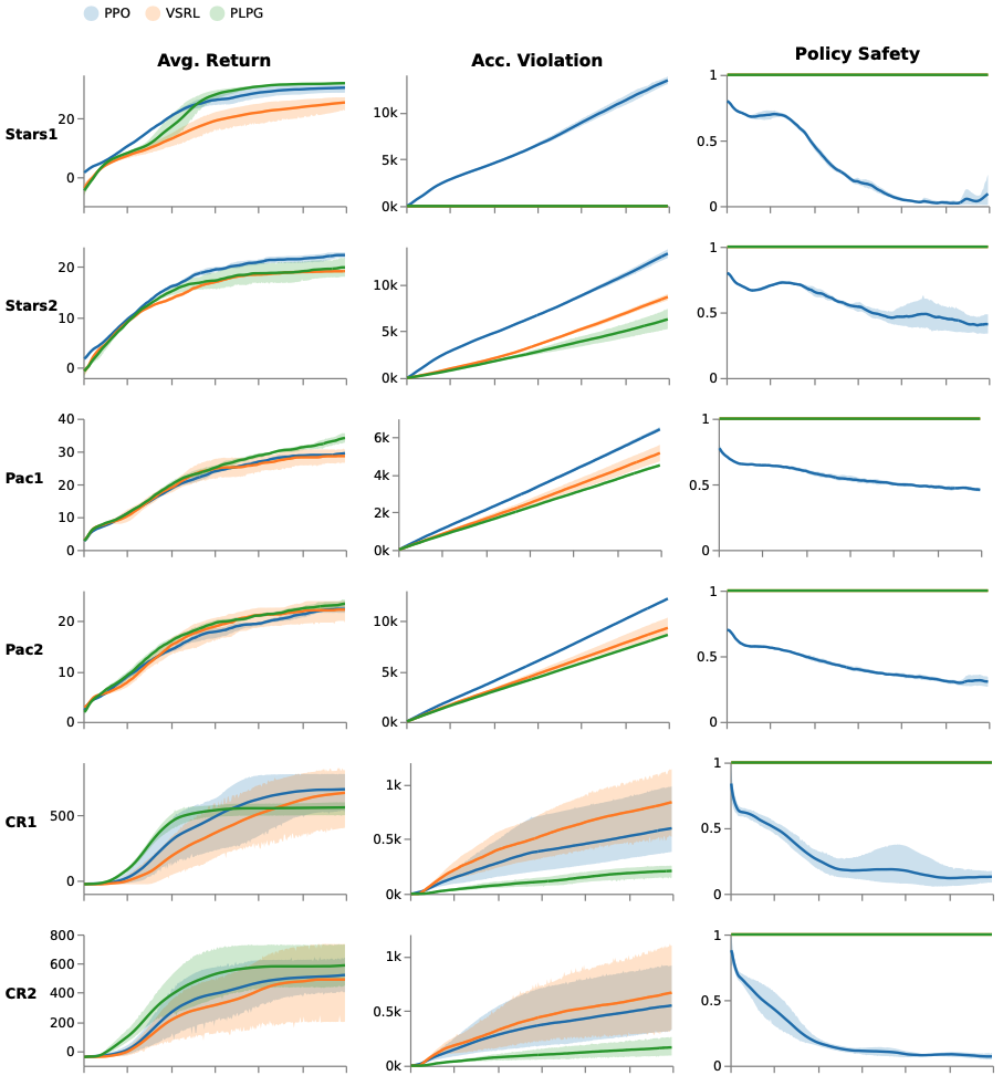
Figure 10: Performance of agents augmented with perfect sensors. Left: The average episodic return. Middle: The cumulative episodic constraint violation. Right: The step-wise policy safety, i.e. $P_{\pi}(\mathtt{safe}|s)$.

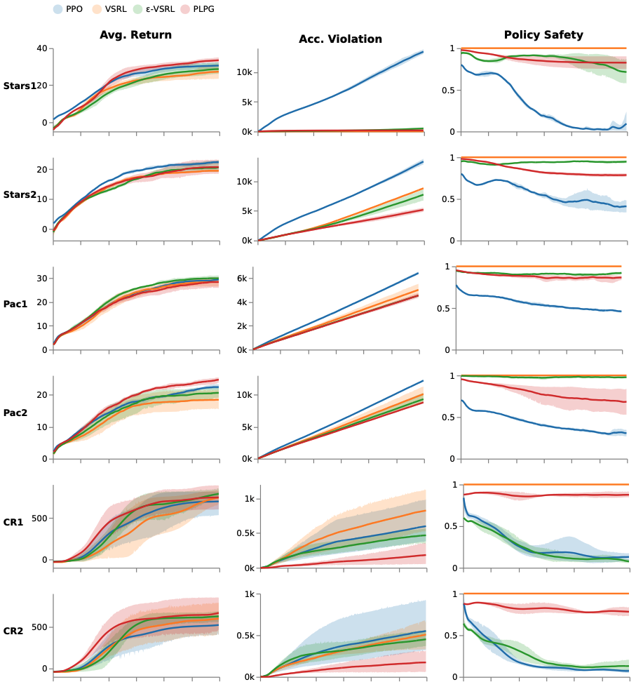
Figure 11: Performance of agents augmented with noisy sensors. Left: The average episodic return. Middle: The cumulative episodic constraint violation. Right: The step-wise policy safety, i.e. $P_{\pi}(\mathtt{safe}|s)$.

References

- Achiam et al. [2017] Joshua Achiam, David Held, Aviv Tamar, and Pieter Abbeel. Constrained policy optimization. In Proceedings of the 34th International Conference on Machine Learning - Volume 70, ICML’17, page 22–31. JMLR.org, 2017.
- Ahmed et al. [2022] Kareem Ahmed, Stefano Teso, Kai-Wei Chang, Guy Van den Broeck, and Antonio Vergari. Semantic probabilistic layers for neuro-symbolic learning. In Advances in Neural Information Processing Systems, 2022.
- Alshiekh et al. [2018] Mohammed Alshiekh, Roderick Bloem, Rüdiger Ehlers, Bettina Könighofer, Scott Niekum, and Ufuk Topcu. Safe reinforcement learning via shielding. AAAI’18/IAAI’18/EAAI’18. AAAI Press, 2018.
- Anderson et al. [2020] Greg Anderson, Abhinav Verma, Isil Dillig, and Swarat Chaudhuri. Neurosymbolic reinforcement learning with formally verified exploration. In Proceedings of the 34th International Conference on Neural Information Processing Systems, NIPS’20, 2020.
- Bastani et al. [2018] Osbert Bastani, Yewen Pu, and Armando Solar-Lezama. Verifiable reinforcement learning via policy extraction. In Proceedings of the 32nd International Conference on Neural Information Processing Systems, NIPS’18, page 2499–2509. Curran Associates Inc., 2018.
- Brockman et al. [2016] Greg Brockman, Vicki Cheung, Ludwig Pettersson, Jonas Schneider, John Schulman, Jie Tang, and Wojciech Zaremba. Openai gym, 2016.
- Camacho et al. [2019] Alberto Camacho, Rodrigo Toro Icarte, Toryn Q. Klassen, Richard Valenzano, and Sheila A. McIlraith. Ltl and beyond: Formal languages for reward function specification in reinforcement learning. In Proceedings of the Twenty-Eighth International Joint Conference on Artificial Intelligence, IJCAI-19, 7 2019.
- Carr et al. [2022] Steven Carr, Nils Jansen, Sebastian Junges, and Ufuk Topcu. Safe reinforcement learning via shielding under partial observability, 2022.
- Cheng et al. [2019] Richard Cheng, Gábor Orosz, Richard M. Murray, and Joel W. Burdick. End-to-end safe reinforcement learning through barrier functions for safety-critical continuous control tasks. AAAI’19/IAAI’19/EAAI’19. AAAI Press, 2019.
- Dalal et al. [2018] Gal Dalal, Krishnamurthy Dvijotham, Matej Vecerik, Todd Hester, Cosmin Paduraru, and Yuval Tassa. Safe exploration in continuous action spaces, 2018.
- Darwiche [2003] Adnan Darwiche. A differential approach to inference in bayesian networks. J. ACM, 50(3):280–305, may 2003.
- De Giacomo et al. [2021] Giuseppe De Giacomo, Luca Iocchi, Marco Favorito, and Fabio Patrizi. Foundations for restraining bolts: Reinforcement learning with ltlf/ldlf restraining specifications. Proceedings of the International Conference on Automated Planning and Scheduling, 29(1):128–136, 2021.
- De Raedt and Kimmig [2015] Luc De Raedt and Angelika Kimmig. Probabilistic (logic) programming concepts. Mach. Learn., 100(1):5–47, 2015.
- De Raedt et al. [2016] Luc De Raedt, Kristian Kersting, Sriraam Natarajan, and David Poole. Statistical Relational Artificial Intelligence: Logic, Probability, and Computation, volume 32 of Synthesis Lectures on Artificial Intelligence and Machine Learning. Morgan & Claypool, 2016.
- Den Hengst et al. [2022] Floris Den Hengst, Vincent François-Lavet, Mark Hoogendoorn, and Frank van Harmelen. Planning for potential: Efficient safe reinforcement learning. Mach. Learn., 111(6):2255–2274, 2022.
- Fernández and Veloso [2006] Fernando Fernández and Manuela Veloso. Probabilistic policy reuse in a reinforcement learning agent. AAMAS ’06. Association for Computing Machinery, 2006.
- Fierens et al. [2015] Daan Fierens, Guy Van den Broeck, Joris Renkens, Dimitar Shterionov, Bernd Gutmann, Ingo Thon, Gerda Janssens, and Luc De Raedt. Inference and learning in probabilistic logic programs using weighted Boolean formulas. Theory and Practice of Logic Programming, 15:358–401, 5 2015.
- García and Fernández [2015] Javier García and Fernando Fernández. A comprehensive survey on safe reinforcement learning. Journal of Machine Learning Research, 16:1437–1480, 2015.
- García and Fernández [2019] Javier García and Fernando Fernández. Probabilistic policy reuse for safe reinforcement learning. ACM Trans. Auton. Adapt. Syst., 13(3), 2019.
- Giacobbe et al. [2021] Mirco Giacobbe, Mohammadhosein Hasanbeig, Daniel Kroening, and Hjalmar Wijk. Shielding atari games with bounded prescience. In Proceedings of the 20th International Conference on Autonomous Agents and MultiAgent Systems, AAMAS ’21, 2021.
- Harris and Schaub [2020] Andrew Harris and Hanspeter Schaub. Spacecraft command and control with safety guarantees using shielded deep reinforcement learning. AIAA Scitech 2020 Forum, 1 PartF, 2020.
- Hasanbeig et al. [2019] M. Hasanbeig, Y. Kantaros, A. Abate, D. Kroening, G. J. Pappas, and I. Lee. Reinforcement learning for temporal logic control synthesis with probabilistic satisfaction guarantees. In 2019 IEEE 58th Conference on Decision and Control (CDC), 2019.
- Hill et al. [2018] Ashley Hill, Antonin Raffin, Maximilian Ernestus, Adam Gleave, Anssi Kanervisto, Rene Traore, Prafulla Dhariwal, Christopher Hesse, Oleg Klimov, Alex Nichol, Matthias Plappert, Alec Radford, John Schulman, Szymon Sidor, and Yuhuai Wu. Stable baselines. https://github.com/hill-a/stable-baselines, 2018.
- Hunt et al. [2021] Nathan Hunt, Nathan Fulton, Sara Magliacane, Trong Nghia Hoang, Subhro Das, and Armando Solar-Lezama. Verifiably safe exploration for end-to-end reinforcement learning. In Proceedings of the 24th International Conference on Hybrid Systems: Computation and Control, HSCC ’21, 2021.
- Jansen et al. [2020] Nils Jansen, Bettina Könighofer, Sebastian Junges, Alex Serban, and Roderick Bloem. Safe reinforcement learning using probabilistic shields. In 31st International Conference on Concurrency Theory, CONCUR 2020, 2020.
- Jiang et al. [2021] Yuqian Jiang, Suda Bharadwaj, Bo Wu, Rishi Shah, Ufuk Topcu, and Peter Stone. Temporal-logic-based reward shaping for continuing reinforcement learning tasks. Proceedings of the AAAI Conference on Artificial Intelligence, 35(9):7995–8003, 2021.
- Junges et al. [2021] Sebastian Junges, Nils Jansen, and Sanjit A. Seshia. Enforcing almost-sure reachability in pomdps. In Computer Aided Verification. Springer International Publishing, 2021.
- Kalweit et al. [2020] Gabriel Kalweit, Maria Huegle, Moritz Werling, and Joschka Boedecker. Deep Constrained Q-learning. 2020.
- Karkus et al. [2017] Peter Karkus, David Hsu, and Wee Sun Lee. Qmdp-net: Deep learning for planning under partial observability. In Proceedings of the 31st International Conference on Neural Information Processing Systems, NIPS’17. Curran Associates Inc., 2017.
- Kimura et al. [2021] Daiki Kimura, Subhajit Chaudhury, Akifumi Wachi, Ryosuke Kohita, Asim Munawar, Michiaki Tatsubori, and Alexander Gray. Reinforcement Learning with External Knowledge by using Logical Neural Networks. 2021.
- Li and Bastani [2020] Shuo Li and Osbert Bastani. Robust Model Predictive Shielding for Safe Reinforcement Learning with Stochastic Dynamics. Proceedings - IEEE International Conference on Robotics and Automation, 2020.
- Memarian et al. [2021] Farzan Memarian, Wonjoon Goo, Rudolf Lioutikov, Ufuk Topcu, and Scott Niekum. Self-Supervised Online Reward Shaping in Sparse-Reward Environments. 2021.
- Mnih et al. [2016] Volodymyr Mnih, Adrià Puigdomènech Badia, Mehdi Mirza, Alex Graves, Timothy P. Lillicrap, Tim Harley, David Silver, and Koray Kavukcuoglu. Asynchronous methods for deep reinforcement learning. 2016.
- Moldovan and Abbeel [2012] Teodor Mihai Moldovan and Pieter Abbeel. Safe exploration in markov decision processes. In Proceedings of the 29th International Coference on International Conference on Machine Learning, ICML’12. Omnipress, 2012.
- Nitti et al. [2016] Davide Nitti, Tinne De Laet, and Luc De Raedt. Probabilistic logic programming for hybrid relational domains. Machine Learning, 103:407–449, 2016.
- Pham et al. [2018] Tu-Hoa Pham, Giovanni De Magistris, and Ryuki Tachibana. Optlayer - practical constrained optimization for deep reinforcement learning in the real world. In 2018 IEEE International Conference on Robotics and Automation (ICRA), pages 6236–6243, 2018.
- Pishro-Nik [2014] H. Pishro-Nik. Introduction to Probability, Statistics, and Random Processes. Kappa Research, LLC, 2014.
- Ray et al. [2019] Alex Ray, Joshua Achiam, and Dario Amodei. Benchmarking Safe Exploration in Deep Reinforcement Learning. arXiv preprint, pages S. 1–6, 2019.
- Robert et al. [1999] Christian P Robert, George Casella, and George Casella. Monte Carlo statistical methods, volume 2. Springer, 1999.
- Schulman et al. [2015] John Schulman, Sergey Levine, Pieter Abbeel, Michael Jordan, and Philipp Moritz. Trust region policy optimization. In Proceedings of the 32nd International Conference on Machine Learning, Proceedings of Machine Learning Research. PMLR, 2015.
- Schulman et al. [2017] John Schulman, Filip Wolski, Prafulla Dhariwal, Alec Radford, and Oleg Klimov. Proximal policy optimization algorithms, 2017.
- Schulman et al. [2018] John Schulman, Philipp Moritz, Sergey Levine, Michael Jordan, and Pieter Abbeel. High-dimensional continuous control using generalized advantage estimation, 2018.
- Sutton and Barto [2018] Richard S. Sutton and Andrew G. Barto. Reinforcement Learning: An Introduction. A Bradford Book, 2018.
- Sutton et al. [2000] Richard S Sutton, David McAllester, Satinder Singh, and Yishay Mansour. Policy gradient methods for reinforcement learning with function approximation. In Advances in Neural Information Processing Systems, volume 12. MIT Press, 2000.
- Tessler et al. [2019] Chen Tessler, Daniel J. Mankowitz, and Shie Mannor. Reward constrained policy optimization. In 7th International Conference on Learning Representations, ICLR. OpenReview.net, 2019.
- Verma et al. [2019] Abhinav Verma, Hoang M. Le, Yisong Yue, and Swarat Chaudhuri. Imitation-projected programmatic reinforcement learning. In Proceedings of the 33rd International Conference on Neural Information Processing Systems, 2019.
- Xu et al. [2018] Jingyi Xu, Zilu Zhang, Tal Friedman, Yitao Liang, and Guy Van den Broeck. A semantic loss function for deep learning with symbolic knowledge. In Proceedings of the 35th International Conference on Machine Learning, ICML’18. PMLR, 2018.