The area of rhumb polygons

Abstract

The formula for the area of a rhumb polygon, a polygon whose edges are rhumb lines on an ellipsoid of revolution, is derived and a method is given for computing the area accurately. This paper also points out that standard methods for computing rhumb lines give inaccurate results for nearly east- or west-going lines; this problem is remedied by the systematic use of divided differences.

1 Introduction

A rhumb line (also called a loxodrome) is a line of constant azimuth on the surface of an ellipsoid, see Figs. 1 and 2. It is important for historical reasons because sailing with a constant compass heading is simpler than sailing the shorter geodesic course; the distinguishing feature of the Mercator projection is that rhumb lines map to straight lines in this projection. The method for computing rhumb lines on a sphere was given by Wright in 1599 and this was extended to an ellipsoid of revolution by Lambert (1772) who derived the ellipsoidal generalization of the Mercator projection. Distances along the rhumb line are then given in terms of the incomplete elliptic integral of the second kind (Legendre, 1811). Subsequent papers on rhumb lines largely focus on simplifications to allow them to be easily computed by navigators at sea.

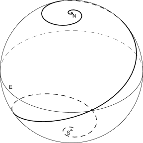
Figure 1: A rhumb line on a sphere illustrating its distinctive characteristic: spiraling infinitely many times around each pole (in the polar stereographic projection, the rhumb line maps to a logarithmic spiral). However, the rhumb line distance between the poles is finite; in this case, the constant azimuth is taken to be $\sec^{-1}3=70.5^{\circ}$ so that this distance is 3 times the distance along the meridian. The rhumb line is viewed in an orthographic projection from a point at latitude $35^{\circ}$; the poles and the equator are labeled “N”, “S”, and “E”.

In this paper we address two issues:

1. Computing rhumb lines accurately for the case of headings close to $\pm 90^{\circ}$. The standard method results in a severe loss of significant bits. This can be avoided by the use of divided differences.

2. Finding the area “under” a rhumb line segment, i.e., the area of the quadrilateral formed by the segment, two meridian arcs, and a segment of the equator. This allows the areas of rhumb polygons to be computed accurately even for very eccentric ellipsoids.

We consider an ellipsoid of revolution with equatorial radius $a$ and polar semi-axis $b$. The shape of the ellipsoid is variously characterized by the flattening $f=(a-b)/a$, the third flattening $n=(a-b)/(a+b)$, the eccentricity squared $e^{2}=(a^{2}-b^{2})/a^{2}$, or the second eccentricity squared $e^{\prime 2}=(a^{2}-b^{2})/b^{2}$. The (geographic) latitude and longitude are denoted by $\phi$ and $\lambda$. The azimuth of a rhumb line, measured clockwise from north is denoted by $\alpha$.

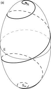
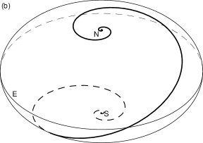
Figure 2: Rhumb lines (a) on a prolate ellipsoid, $b/a=2$, and (b) on an oblate ellipsoid, $b/a=\frac{1}{2}$. The bearing of the rhumb line and the projection match that of Fig. 1.

2 Formulation of the rhumb line problem

Rhumb lines map to straight lines in the Mercator projection because this projection is conformal and because it maps meridians to parallel straight lines. Ellipsoidal effects can be simply introduced using various auxiliary latitudes, the conformal latitude $\chi$, the rectifying latitude $\mu$, the parametric latitude $\beta$, and the authalic latitude $\xi$. In the spherical limit, these four auxiliary latitudes reduce to the geographic latitude $\phi$.

It is possible to convert between these various latitudes accurately (Karney, 2022b) and, in this paper, we treat this as a solved problem. We keep the notation simple by writing, for example, $\mu_{1}$ instead of $\mu(\phi_{1})$.

The Mercator projection maps a point on the earth with longitude $\lambda$ and latitude $\phi$ to a point $(\lambda,\psi)$ on the plane where $\psi$ is the isometric latitude

$$\psi=\mathop{\mathrm{lam}}\nolimits\chi=\mathop{\mathrm{gd}}\nolimits^{-1}\chi=\sinh^{-1}\tan\chi,$$ (1)

$\mathop{\mathrm{lam}}\nolimits\chi$ is the Lambertian function, and its inverse, $\mathop{\mathrm{gd}}\nolimits\psi=\tan^{-1}\sinh\psi$, is the gudermannian function (Olver et al., 2010, §http://dlmf.nist.gov/4.23.viii).

Treating first the inverse rhumb line problem, finding the course $\alpha_{12}$ and length $s_{12}$ of the rhumb line between two points $(\phi_{1},\lambda_{1})$ and $(\phi_{2},\lambda_{2})$, we have simply

$$\alpha_{12} =\tan^{-1}\genfrac{}{}{1.4pt}{0}{\lambda_{12}}{\psi_{12}},$$ (2)

$$\frac{s_{12}}{R} =\mu_{12}\sec\alpha_{12}$$

$$=\frac{\mu_{12}}{\psi_{12}}\sqrt{\lambda_{12}^{2}+\psi_{12}^{2}},$$ (3)

where $R$ is the rectifying radius of the ellipsoid, $\psi_{12}=\psi_{2}-\psi_{1}$, $\mu_{12}=\mu_{2}-\mu_{1}$, $\lambda_{12}=\lambda_{2}-\lambda_{1}$; typically, $\lambda_{12}$ is reduced to the range $[-\pi,\pi]$ (thus giving the course of the shortest rhumb line). The heavy ratio line in Eq. (2) indicates that the quadrant of the arctangent is determined by the signs of the numerator and denominator of the ratio. The distance from the equator to a pole can be expressed in terms of $R$ as

$$\frac{\pi}{2}R=aE(e)=bE(ie^{\prime})=2R_{G}(0,a^{2},b^{2}),$$ (4)

where $E(k)$ is the complete elliptic integral of the second kind (Olver et al., 2010, §http://dlmf.nist.gov/19.2.ii) and $R_{G}(x,y,z)$ is one of the symmetric elliptic integrals (Olver et al., 2010, §http://dlmf.nist.gov/19.16.ii). For small flattening, we can use (Ivory, 1798)

$$R =\frac{a}{1+n}\sum_{j=0}^{\infty}\biggl{(}\frac{(2j-3)!!}{(2j)!!}\biggr{)}^{2}n^{2j}$$

$$=\frac{a}{1+n}\bigl{(}\textstyle 1+\frac{1}{4}n^{2}+\frac{1}{64}n^{4}+\frac{1}{256}n^{6}+O(n^{8})\bigr{)}.$$ (5)

The direct problem is treated similarly. We are given the starting point $(\phi_{1},\lambda_{1})$, the course $\alpha_{12}$, and the distance $s_{12}$ along a rhumb line, and wish to determine the destination $(\phi_{2},\lambda_{2})$. We can write

$$\mu_{12}=\frac{s_{12}}{R}\cos\alpha_{12},$$ (6)

from which we can find $\mu_{2}$, $\phi_{2}$ and $\psi_{2}$. Then we have

$$\lambda_{12} =\psi_{12}\tan\alpha_{12}$$

$$=\frac{s_{12}}{R}\frac{\psi_{12}}{\mu_{12}}\sin\alpha_{12}.$$ (7)

In this formulation, we do not restrict the sign of $s_{12}$; negative distances are allowed in the direct problem. If the value of $\mu_{2}=\mu_{1}+\mu_{12}$ lies outside the normal range for latitudes, $[-\frac{1}{2}\pi,\frac{1}{2}\pi]$, then it should be replaced by its supplement. Because, in this case, the rhumb line has spiraled infinitely many times around the pole, see Figs. 1 and 2, $\lambda_{12}$ is then indeterminate. This is also the outcome if $\mu_{2}=\pm\frac{1}{2}\pi$ because then $\psi_{12}=\pm\infty$ and Eq. (7) gives an indeterminate result.

Both Eqs. (3) and (7) are indeterminate in the limit $\phi_{2}\rightarrow\phi_{1}$, since both $\psi_{12}$ and $\mu_{12}$ vanish. However, we can apply l’Hôpital’s rule and write

$$\frac{\mu_{12}}{\psi_{12}}\rightarrow\frac{\mathrm{d}\mu_{1}}{\mathrm{d}\psi_{1}}=\frac{a\cos\beta_{1}}{R},$$ (8)

where the formula for the derivative follows from the defining differential equations for $\psi$ and $\mu$. Note that $a\cos\beta_{1}$ is the radius of a circle of latitude $\phi_{1}$.

This provides a complete solution for the course of rhumb lines. We can see that by using auxiliary latitudes, the spherical solution is readily generalized to an ellipsoid; Fig. 2 shows rhumb lines on prolate and oblate ellipsoids. In implementing such a solution, we have a choice of using series expansions for converting between auxiliary latitudes, recommended for $\lvert f\rvert\lesssim\frac{1}{100}$, or directly evaluating the formulas for the auxiliary latitudes. Details of both methods are given in Karney (2022b).

When using Eqs. (3) and (7), we are faced with a severe loss of accuracy if $\phi_{2}\approx\phi_{1}$ because then both $\mu_{12}$ and $\psi_{12}$ involve the difference between two nearly equal quantities resulting in catastrophic roundoff errors.

A simple solution, suggested, for example, by Meyer and Rollins (2011), is to extend the treatment of rhumb lines that run exactly along parallels to the case $\phi_{2}\approx\phi_{1}$, i.e., to replace the ratio $\mu_{12}/\psi_{12}$ by the derivative $\mathrm{d}\mu/\mathrm{d}\psi$, Eq. (8), evaluated at the midpoint $\phi={\frac{1}{2}(\phi_{1}+\phi_{2})}$. However this is not entirely satisfactory: you have to pick the transition point where the derivative takes over from the ratio of differences; and, near this transition point, many bits of accuracy will be lost.

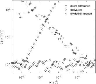
Figure 3: The absolute errors $\delta s_{12}$ in computing $s_{12}$ for rhumb lines on a sphere of radius $a=6400\,\mathrm{km}$, with mean latitude $\frac{1}{2}(\phi_{1}+\phi_{2})=45^{\circ}$, longitude difference $\lambda_{12}=90^{\circ}$, and various values of $\phi_{12}=\phi_{2}-\phi_{1}$. Three methods of computing $\mu_{12}/\psi_{12}$ are compared: the direct ratio of the differences Eq. (3) (plus signs); approximating the ratio by the derivative Eq. (8) (crosses); evaluating the ratio using divided differences Eq. (28) (diamonds). The systematic variation of the errors for the derivative approximation is indicative that this is (for the most part) a truncation error. The random variations for the other cases are due to roundoff. In all three cases, the calculations are carried out in double precision (53 bits in the fraction of the floating-point representation); these are compared with the results of a high (256-bit) precision calculation which are taken to be “exact”.

This conundrum is nicely illustrated by Fig. 3 which shows the errors $\delta s_{12}$ in the computed distance as $\phi_{12}=\phi_{2}-\phi_{1}$ is varied. Here the plus signs and crosses give $\delta s_{12}$ when computing $\mu_{12}/\psi_{12}$ using the ratio of the differences and the mid-point derivative, respectively. Given just these two choices for the calculation, there is an unavoidable degradation in the accuracy for $0.000\,01^{\circ}<\phi_{12}<1^{\circ}$. Selecting $\phi_{12}=0.001^{\circ}$ as the transition point, the maximum error in the distance is about $0.1\,\mathrm{mm}$. This loss of accuracy may not matter in some applications; however, we would wish to avoid such a compromise if possible.

It turns out that we can do substantially better and maintain full double-precision accuracy. Indeed Botnev and Ustinov (2014) provide formulas which allow $\mu_{12}/\psi_{12}$ to be computed accurately; however their treatment of $\psi_{12}$ is somewhat ad hoc and their formula for $\mu_{12}$ applies only for small flattening. The problem can be addressed more simply by using the algebra of divided differences (Kahan and Fateman, 1999). This technique can be used to reduce roundoff errors in a wide range of applications and we detail how it can be applied to computing $\mu_{12}/\psi_{12}$ in Appendix A. The result is illustrated by the diamonds in Fig. 3 which show that the errors using divided differences with double precision are on the order of $1\,\mathrm{nm}$ throughout the range of $\phi_{12}$. This establishes that the conventional approach for computing the distance (the plus signs and the crosses) needlessly loses, in some cases, just over a quarter of the bits of precision in a floating-point number. Using divided differences allows for a single computational method, avoids the tricky business of picking transition points, and maintains full accuracy.

3 The area under a rhumb line

The boundaries of political entities are sometimes defined as oblique “straight” lines, e.g., the border between California and Nevada, the border between Algeria and its southern neighbors, Mauritania and Mali, and the zigzag border between Jordan and Saudi Arabia. It’s often not clear precisely how these lines are defined. Reasonable choices are geodesics (straight on the ellipsoid), rhumb lines (straight in the Mercator projection), or straight lines in some other agreed-upon projection. Borders can also be specified as a circle of latitude (which is, of course, also a rhumb line), for example, the 49th parallel which separates the USA and Canada. Assuming that the border of an entity is defined in terms of rhumb lines, we might wish to compute the resulting area.

This exercise was carried out for geodesic polygons in Karney (2013), where, following Danielsen (1989), the area between a geodesic line segment and the equator was determined. The area of a polygon is then given by summing algebraically the contribution from each of the polygon edges (with an adjustment required for polygons that encircle a pole).

Here, we repeat this exercise by computing $S_{12}$, the area of a rhumb quadrilateral with vertices $(0,\lambda_{1})$, $(0,\lambda_{2})$, $(\phi_{2},\lambda_{2})$, and $(\phi_{1},\lambda_{1})$ made up of two meridian arcs, an equatorial segment, and a general rhumb segment. With this result in hand, we can compute the area of arbitrary rhumb polygons. The area for a particular segment is given by

$$S_{12}=\int_{\lambda_{1}}^{\lambda_{2}}c^{2}\sin\xi\,\mathrm{d}\lambda,$$ (9)

where $\xi$ is the authalic latitude and

$$c^{2}=\frac{a^{2}}{2}+\frac{b^{2}}{2}\frac{\tanh^{-1}e}{e}$$ (10)

is the authalic radius squared. We change the variable of integration in Eq. (9) first from $\lambda$ to $\psi$, using $\mathrm{d}\lambda/\mathrm{d}\psi=\lambda_{12}/\psi_{12}$, and then to $\chi$, using $\mathrm{d}\psi/\mathrm{d}\chi=\sec\chi$, to obtain

$$S_{12}=c^{2}\lambda_{12}\frac{p_{12}}{\psi_{12}},$$ (11)

where $p_{12}=p(\chi_{2})-p(\chi_{1})$ and

$$p(\chi)=\int\sin\xi\sec\chi\,\mathrm{d}\chi.$$ (12)

In the limit, $\chi_{2}\rightarrow\chi_{1}$, we have (applying l’Hôpital’s rule again)

$$S_{12}\rightarrow c^{2}\lambda_{12}\frac{\mathrm{d}p(\chi_{1})/\mathrm{d}\chi_{1}}{\mathrm{d}\psi_{1}/\mathrm{d}\chi_{1}}=c^{2}\lambda_{12}\sin\xi_{1},$$ (13)

the well-known result for the area under a segment of a circle of latitude.

In the spherical limit, we have $\sin\xi\rightarrow\sin\chi$ and the integrand in Eq. (12) becomes $\tan\chi$. This suggests that we separate $p(\chi)$ into a spherical contribution and an ellipsoidal correction by writing

$$p(\chi) =p_{0}(\chi)+p_{\chi}(\chi),$$ (14)

$$p_{0}(\chi) =\int\tan\chi\,\mathrm{d}\chi$$

$$=\log\sec\chi=\sinh^{-1}\frac{\tan\chi\sin\chi}{2},$$ (15)

$$p_{\chi}(\chi) =\int q_{\chi}(\chi)\,\mathrm{d}\chi,$$ (16)

$$q_{\chi}(\chi) =\frac{\sin\xi-\sin\chi}{\cos\chi}.$$ (17)

The spherical term $p_{0}(\chi)$ is singular for $\chi\rightarrow\frac{1}{2}\pi$; this just reflects the rapid encircling of the pole by a rhumb line as it approaches a pole. The second expression for the integral in Eq. (15) avoids roundoff errors for small $\chi$.

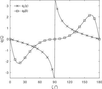
Figure 4: The integrands $q_{\chi}(\chi)$ and $q_{\beta}(\beta)$, Eqs. (17) and (19), for the ellipsoidal correction for the area integral marked, respectively, with crosses and squares. The case illustrated is for a prolate ellipsoid with $n=-\frac{5}{8}$. Note that $\int_{0}^{\pi/2}q_{\chi}(\chi)\,\mathrm{d}\chi=\int_{0}^{\pi/2}q_{\beta}(\beta)\,\mathrm{d}\beta$.

We are now confronted with the evaluation of $p_{\chi}(\chi)$, Eq. (16). Almost certainly the integral cannot be carried out in closed form. However, since $q_{\chi}(\chi)$ is a periodic function (with period $\pi$), it is natural to develop it as a Fourier series allowing the integral to be simply performed. Unfortunately, even though the integrand $q_{\chi}(\chi)$, Eq. (17), is a well-behaved function of $\chi$, it can vary strongly particularly for prolate ellipsoids; for example, the curve marked with crosses in Fig. 4 shows $q_{\chi}(\chi)$ for $n=-\frac{5}{8}$ or $b/a=13/3$. As a result, the Fourier series converges slowly with many terms needed to yield an accurate result.

We address this problem by changing the variable of integration in Eq. (16) from $\chi$ to the parametric latitude $\beta$. Thus we replace Eq. (16) by

$$p_{\beta}(\beta)=\int q_{\beta}(\beta)\,\mathrm{d}\beta,$$ (18)

with

$$q_{\beta}(\beta)=q_{\chi}(\chi)\frac{\mathrm{d}\chi}{\mathrm{d}\beta}=(1-f)\frac{\sin\xi-\sin\chi}{\cos\phi},$$ (19)

where we have used

$$\frac{\mathrm{d}\chi}{\mathrm{d}\beta}=(1-f)\frac{\cos\chi}{\cos\phi}.$$ (20)

Our notation here is such that $p_{\beta}(\beta)=p_{\beta}\bigl{(}\beta(\chi)\bigr{)}=p_{\chi}(\chi)$. The curve marked with squares in Fig. 4 shows $q_{\beta}(\beta)$ for $n=-\frac{5}{8}$ confirming that it varies more smoothly than $q_{\chi}(\chi)$. Finally, we write

$$p_{\beta}(\beta)=\sum_{l=1}^{L}P_{l}\cos 2l\beta,$$ (21)

where $P_{l}$ are the coefficients of the Fourier series for $p_{\beta}(\beta)$ and $L$ is picked sufficiently large that we may approximate $P_{l}=0$ for $l>L$. For the case illustrated in Fig. 4, $n=-\frac{5}{8}$, taking $L=50$ allows $q_{\beta}(\beta)$ to be evaluated with full double-precision accuracy; in contrast, we would have needed to include $L=L_{\chi}=3993$ terms if we were fitting $q_{\chi}(\chi)$. Since $p_{\beta}(\beta)$ is an indefinite integral, Eq. (18), we pick the constant of integration such that $P_{0}=0$ and the Fourier series, Eq. (21), starts with the $l=1$ term.

If the flattening of the ellipsoid is small, we can expand $q_{\beta}(\beta)$ as a Taylor series in $n$; this allows the integral to be performed analytically, giving the following series approximations for $P_{l}$:

$$\mathbf{P}^{(L)}=\mathsf{Q}^{(L)}\cdot\mathbf{N}^{(L)}+O(n^{L+1}),$$ (22)

where

$$\mathbf{P}^{(L)} =[P_{1},P_{2},P_{3},\ldots,P_{L}]^{\mathsf{T}},$$ (23)

$$\mathbf{N}^{(L)} =[n,n^{2},n^{3},\ldots,n^{L}]^{\mathsf{T}}$$ (24)

are column vectors of length $L$ and, for $L=6$,

$$\mathsf{Q}^{(6)}=\begin{bmatrix}-\frac{1}{3}&\frac{22}{45}&-\frac{398}{945}&\frac{596}{2025}&-\frac{102614}{467775}&\frac{138734126}{638512875}\\ &\frac{1}{5}&-\frac{118}{315}&\frac{1543}{4725}&-\frac{24562}{155925}&\frac{17749373}{425675250}\\ &&-\frac{17}{315}&\frac{152}{945}&-\frac{38068}{155925}&\frac{1882432}{8513505}\\ &&&\frac{5}{252}&-\frac{752}{10395}&\frac{268864}{2027025}\\ &&&&-\frac{101}{17325}&\frac{62464}{2027025}\\ &&&&&\frac{11537}{4054050}\end{bmatrix}$$ (25)

is an $L\times L$ upper triangular matrix. (Note that $P_{l}=O(n^{l})$, so that all the neglected, $l>L$, terms in the Fourier series for $p_{\beta}(\beta)$ are $O(n^{L+1})$.) Here the necessary algebra for carrying out the Taylor expansion and subsequent integration was performed by Maxima (2022). Truncating the expansion at $L=6$ as shown here gives full double-precision accuracy for $\lvert f\rvert\leq\frac{1}{100}$.

The radius of convergence of this series can be estimated by examining the coefficients $\mathsf{Q}^{(40)}$, which indicates convergence for $\lvert n|\lesssim 1$, i.e., for all eccentricities. Nevertheless, it is wise to limit the series method to reasonably small values of the flattening, say $\lvert f\rvert\leq\frac{1}{10}$ (for which $L=12$ gives full accuracy).

This completes the formulation for the area under a rhumb line for the case of small flattening. For larger eccentricities, we adopt the technique introduced in Karney (2022a), namely to evaluate the Fourier coefficients $P_{l}$ appearing in Eq. (21) at run time by performing a discrete Fourier transform (DFT) on a set of evenly spaced samples of $q_{\beta}(\beta)$. The details of this approach are given in Appendix C. Here, we merely note that a modest number of Fourier coefficients allows the area to be computed with full double-precision accuracy (see Table 1 in Appendix C).

The term $p_{12}/\psi_{12}$ appearing in Eq. (11) presents precisely the same issues as $\mu_{12}/\psi_{12}$ in Eq. (3), namely taking the ratio of two differences which is potentially subject to an unacceptable loss of accuracy. If $\phi_{2}=\phi_{1}$, we can use Eq. (13); but in the general case, we need again to use divided differences as explained in Appendix C.

It is interesting to compare this result, Eqs. (11) and (14), with the corresponding result for the geodesic problem, Eqs. (58), (59), and (61) in Karney (2013). In both cases, we have separated the area into a spherical contribution, which has singular behavior for paths that pass close to a pole, and an ellipsoidal correction.

However, in distinction to the geodesic problem, the longitude enters the formula for the area, Eq. (11), as a multiplicative factor, $\lambda_{12}$; this reflects the simple geometry of rhumb lines. As a consequence, $p_{12}$ depends just on the latitudes of the endpoints and on the flattening of the ellipsoid. This allows the coefficients $P_{l}$ in Eq. (21) to be evaluated as soon as the flattening is specified. For the geodesic problem, this was not possible, because the ellipsoidal correction, Eq. (61) in Karney (2013), involves both the flattening and the equatorial azimuth of the geodesic inextricably linked together.

4 Conclusions

We have provided a method for computing the area under a segment of a rhumb line. The sum of the signed contributions for all the segments making up a rhumb polygon gives the area of the polygon. As with geodesic polygons (Karney, 2013), a simple adjustment of the sum is required if the polygon includes a pole. This result for the area is new. Freire and de Vasconcello (2010) have also considered the area of rhumb polygons, but their approach involves breaking up the edges into sufficiently short segments so that Simpson’s method can be applied: the cost of the area evaluation is then proportional to the perimeter of the polygon. In contrast, the cost of the method described here is proportional to the number of vertices in the polygon. Remarkably, the comparatively simple result for a sphere, when Eqs. (14) and (15) reduce to $p(\chi)=\log\sec\chi$, is also new.

Key to maintaining accuracy in this work is the use of divided differences. Although these techniques are well established (Kahan and Fateman, 1999), they have been largely overlooked in geodetic applications. The application of divided differences to Clenshaw summation is also new.

The methods described here were implemented as part of GeographicLib (Karney, 2023) in 2014; however, the area calculations were based on the Taylor expansion of $p_{\chi}(\chi)$ and were therefore limited to small flattenings. For this paper, the routines were reimplemented to utilize the development of auxiliary latitudes given in Karney (2022b), to improve the treatment of the area integral by the change of variables from $\beta$ to $\chi$, and to compute the coefficients for the area integral using a DFT which provided accurate results for the area for highly eccentric ellipsoids. The interface consists of

• C++ classes Rhumb and RhumbLine to solve inverse and direct rhumb line problems;

• a command-line utility RhumbSolve which provides a convenient front end to these classes;

• a command-line utility Planimeter to compute the area of geodesic and rhumb polygons;

• online versions of these tools are also available at https://geographiclib.sourceforge.io/cgi-bin/RhumbSolve and https://geographiclib.sourceforge.io/cgi-bin/Planimeter.

This reimplementation is included in version 2.2 of GeographicLib.

Supplementary data

The following files are provided in

Series expansions for computing rhumb areas,
doi:10.5281/zenodo.7685484,

as supplementary data for this paper:

• rhumbarea.mac: the Maxima code used to obtain the series expansions for $\mathbf{P}^{(L)}$, Eq. (22). Instructions for using this code are included in the file.

• auxlvals40.mac: The series for conversions between auxiliary latitudes which is required by rhumbarea.mac. This is a copy of a file provided in Karney (2022c).

• rhumbvals40.mac: The matrix $\mathsf{Q}$ produced by rhumbarea.mac for $L=40$ in a form suitable for loading into Maxima.

• rhumbvals{6,16,40}.m: The matrix $\mathsf{Q}$ in Octave/MATLAB notation for $L=6$ and $16$ (using exact fractions) and $L=40$ (written as floating-point numbers). rhumbvals6.m reproduces Eq. (25) in “machine-readable” form. rhumbvals40.m can be used to estimate the radii of convergence of Eq. (22). The format of these files is sufficiently simple that they can be easily adapted for any computer language.

Appendix A Use of divided differences

Here I explore how to compute expressions such as $\mu_{12}/\psi_{12}$, which appears in Eqs. (3) and (7), in a way that maintains accuracy. Such expressions can be treated in a systematic way using the algebra of divided differences; the subject is discussed in detail by Kahan and Fateman (1999, henceforth referred to as KF). The divided difference of $f(x)$ is defined by

$$\mathord{\ooalign{$\triangle$\cr\hfil$\mid$\hfil\cr}}[f](x,y)=\begin{cases}df(x)/dx,&\text{if $x=y$,}\\[2.15277pt] \displaystyle\frac{f(y)-f(x)}{y-x},&\text{otherwise.}\end{cases}$$ (26)

The second form above can be used in a computation provided that $x$ and $y$ are sufficiently far apart. The key is to recast this expression into one that avoids excessive roundoff error when $y\approx x$.

Many readers will already be familiar with suitable substitutions for some cases, e.g.,

$$\mathord{\ooalign{$\triangle$\cr\hfil$\mid$\hfil\cr}}[\sin](x,y)={\textstyle\cos\frac{1}{2}(x+y)}\frac{\sin\frac{1}{2}(y-x)}{\frac{1}{2}(y-x)},$$ (27)

which can be evaluated accurately if $y\approx x$ even if the relative error in $y-x$ is significant; because the last factor above varies slowly near $y-x=0$, this error in the divided difference depends only on the absolute error in $y-x$. Section 1.4 in KF provides a set of rules which allow the technique to be applied to a wide range of problems. In particular, suitable divided difference formulas are given for all the elementary functions.

If we regard $\mu$ and $\psi$ as functions of $\chi$, we can write

$$\frac{\mu_{12}}{\psi_{12}}=\frac{\mathord{\ooalign{$\triangle$\cr\hfil$\mid$\hfil\cr}}[\mu](\chi_{1},\chi_{2})}{\mathord{\ooalign{$\triangle$\cr\hfil$\mid$\hfil\cr}}[\psi](\chi_{1},\chi_{2})}.$$ (28)

In the spherical limit, where $\mu=\chi$, the numerator reduces to unity. Therefore we start by considering the denominator, which can be expressed as

$$\mathord{\ooalign{$\triangle$\cr\hfil$\mid$\hfil\cr}}[\psi](\chi_{1},\chi_{2})=\mathord{\ooalign{$\triangle$\cr\hfil$\mid$\hfil\cr}}[\sinh^{-1}](\tan\chi_{1},\tan\chi_{2})\\ \times\mathord{\ooalign{$\triangle$\cr\hfil$\mid$\hfil\cr}}[\tan](\chi_{1},\chi_{2}),$$ (29)

where I have applied the chain rule

$$\mathord{\ooalign{$\triangle$\cr\hfil$\mid$\hfil\cr}}[f\circ g](x,y)=\mathord{\ooalign{$\triangle$\cr\hfil$\mid$\hfil\cr}}[f]\bigl{(}g(x),g(y)\bigr{)}\,\mathord{\ooalign{$\triangle$\cr\hfil$\mid$\hfil\cr}}[g](x,y)$$ (30)

(here $f\circ g$ refers to functional composition) to Eq. (1). Using $\tan\chi$ as the independent variable (instead of $\chi$) allows us to represent accurately values of $\chi$ close to $0$ and $\pm\frac{1}{2}\pi$; thus we use the inverse function rule,

$$\mathord{\ooalign{$\triangle$\cr\hfil$\mid$\hfil\cr}}[f^{-1}](x,y)=1/\mathord{\ooalign{$\triangle$\cr\hfil$\mid$\hfil\cr}}[f]\bigl{(}f^{-1}(x),f^{-1}(y)\bigr{)},$$ (31)

to rewrite Eq. (29) as

$$\mathord{\ooalign{$\triangle$\cr\hfil$\mid$\hfil\cr}}[\psi](\chi_{1},\chi_{2})=\frac{\mathord{\ooalign{$\triangle$\cr\hfil$\mid$\hfil\cr}}[\sinh^{-1}](\tan\chi_{1},\tan\chi_{2})}{\mathord{\ooalign{$\triangle$\cr\hfil$\mid$\hfil\cr}}[\tan^{-1}](\tan\chi_{1},\tan\chi_{2})}.$$ (32)

Note that the chain rule and inverse function rules, Eqs. (30) and (31), are direct analogs of the corresponding rules for derivatives. Equation (32) can be evaluated using the formulas from KF:

$$\mathord{\ooalign{$\triangle$\cr\hfil$\mid$\hfil\cr}}[\sinh^{-1}](x,y) =\sinh^{-1}\biggl{(}\frac{(y-x)(x+y)}{x\sqrt{1+y^{2}}+y\sqrt{1+x^{2}}}\biggr{)}$$ (35)

$$\qquad{}\times\frac{1}{y-x},$$ (36)

$$\mathord{\ooalign{$\triangle$\cr\hfil$\mid$\hfil\cr}}[\tan^{-1}](x,y) =\frac{1}{y-x}\tan^{-1}\frac{y-x}{1+xy}.$$ (39)

For a sphere, where $\mathord{\ooalign{$\triangle$\cr\hfil$\mid$\hfil\cr}}[\mu](\chi_{1},\chi_{2})=1$, Eq. (3) can now be evaluated using Eqs. (28) and (32). Repeating the numerical experiment of Fig. (3), the roundoff errors using divided differences are shown as diamonds; this confirms that this method is effective in dramatically reducing the numerical error.

I’ve only included the basic results in Eqs. (36) and (39); KF supplement these with the derivatives if $y-x$ vanishes or the direct ratios if $x$ and $y$ have opposite signs. Also, it is wise to ensure that correct results are returned in “corner cases”, e.g., $x=0$ and $y=\infty$.

Turning now to the numerator of Eq. (28), $\mathord{\ooalign{$\triangle$\cr\hfil$\mid$\hfil\cr}}[\mu](\chi_{1},\chi_{2})$. We distinguish two cases: if the flattening of the ellipsoid is small, say $\lvert f\rvert\leq\frac{1}{100}$, then we can use a sixth-order trigonometric series to convert between $\chi$ and $\mu$. This can be evaluated using Clenshaw summation and to compute the divided difference we need to extend Clenshaw summation. Since this method is generally useful, we address this separately in Appendix B.

For arbitrary flattening, we recast Eq. (28) as

$$\frac{\mu_{12}}{\psi_{12}}=\frac{\mathord{\ooalign{$\triangle$\cr\hfil$\mid$\hfil\cr}}[\mu](\beta_{1},\beta_{2})\,\mathord{\ooalign{$\triangle$\cr\hfil$\mid$\hfil\cr}}[\beta](\phi_{1},\phi_{2})}{\mathord{\ooalign{$\triangle$\cr\hfil$\mid$\hfil\cr}}[\psi](\phi_{1},\phi_{2})},$$ (40)

and apply divided differences to

$$\beta(\phi) =\tan^{-1}\bigl{(}(1-f)\tan\phi\bigr{)},$$ (41)

$$\mu(\beta) =\frac{bE(\beta,ie^{\prime})}{R},$$ (42)

$$\psi(\phi) =\mathop{\mathrm{lam}}\nolimits\phi-e\tanh^{-1}(e\sin\phi),$$ (43)

where $E(x,k)$ is the incomplete elliptic integral of the second kind (Olver et al., 2010, §http://dlmf.nist.gov/19.2.ii). For Eqs. (41) and (43), this is just a routine exercise applying the results of KF.

KF do not provide a formula for $\mathord{\ooalign{$\triangle$\cr\hfil$\mid$\hfil\cr}}[E](x,y;k)$; they do however note “Examination of ‘addition formulas’ may provide some suggestions for divided differences of additional special functions.” Indeed, the necessary addition formula is found in Olver et al. (2010, Eq. http://dlmf.nist.gov/19.11.E2). With the substitutions $\theta=y$, $\phi=-x$, $\psi=z$, this can be converted to the following divided difference formula,

$$\mathord{\ooalign{$\triangle$\cr\hfil$\mid$\hfil\cr}}[E](x,y;k)=\begin{cases}\sqrt{1-k^{2}\sin^{2}x},&\text{if $x=y$,}\\[2.15277pt] \displaystyle\frac{E(y,k)-E(x,k)}{y-x},&\text{if $xy\leq 0$,}\\[2.15277pt] \displaystyle\biggl{(}\frac{E(z,k)}{\sin z}-k^{2}\sin x\sin y\biggr{)}\\ \qquad\displaystyle{}\times\frac{\sin z}{y-x},&\text{otherwise,}\end{cases}$$ (44)

where the angle $z$ is given by

$$z =\tan^{-1}\genfrac{}{}{1.4pt}{0}{2t}{(1-t)(1+t)},$$ (45)

$$t =\frac{(y-x)\mathord{\ooalign{$\triangle$\cr\hfil$\mid$\hfil\cr}}[\sin](x,y)}{\sin x\sqrt{1-k^{2}\sin^{2}y}+\sin y\sqrt{1-k^{2}\sin^{2}x}}$$ (48)

$$\qquad{}\times\frac{\sin x+\sin y}{\cos x+\cos y}.$$ (49)

(Note that the quantity $t$ is just $\tan\frac{1}{2}z$.) This formula is restricted to the case $\lvert x\rvert\leq\frac{1}{2}\pi$ and $\lvert y\rvert\leq\frac{1}{2}\pi$. It is best used for $k^{2}<0$ so that the two terms in large parentheses have the same sign; this is the case for an oblate ellipsoid ($e^{\prime 2}>0$), since $k^{2}=-e^{\prime 2}<0$. For a prolate ellipsoid ($e^{2}<0$), we can apply finite differences to $\mu^{\prime}(\beta^{\prime})$ (the primes indicate the complementary angles), where

$$\mathord{\ooalign{$\triangle$\cr\hfil$\mid$\hfil\cr}}[\mu](\beta_{1},\beta_{2}) =\mathord{\ooalign{$\triangle$\cr\hfil$\mid$\hfil\cr}}[\mu^{\prime}](\beta^{\prime}_{1},\beta^{\prime}_{2}),$$ (54)

$$\mu^{\prime}(\beta^{\prime}) =\frac{aE(\beta^{\prime},e)}{R},$$ (55)

and once again we have $k^{2}=e^{2}<0$.

We have given here a cursory examination of using divided differences for the ellipsoid with arbitrary flattening. Full details are available in the implementation described in Sec. 4.

Appendix B Divided differences for Clenshaw summation

The numerator of Eq. (28) is $\mathord{\ooalign{$\triangle$\cr\hfil$\mid$\hfil\cr}}[\mu](\chi_{1},\chi_{2})$. Here, we examine evaluating $\mathord{\ooalign{$\triangle$\cr\hfil$\mid$\hfil\cr}}[\eta](\zeta_{1},\zeta_{2})$ for any two auxiliary latitudes $\zeta$ and $\eta$ in the limit of small flattening. In this case, we can approximate (Karney, 2022b)

$$\eta(\zeta) =\zeta+\Delta\eta(\zeta)+O(n^{L+1}),$$ (56)

$$\Delta\eta(\zeta) =\sum_{l=1}^{L}C_{l}\sin 2l\zeta,$$ (57)

where choosing $L=6$ suffices to provide accurate results for $\lvert f\rvert\leq\frac{1}{150}$. The additive property of divided differences lets us write

$$\mathord{\ooalign{$\triangle$\cr\hfil$\mid$\hfil\cr}}[\eta](\zeta_{1},\zeta_{2})=1+\mathord{\ooalign{$\triangle$\cr\hfil$\mid$\hfil\cr}}[\Delta\eta](\zeta_{1},\zeta_{2}).$$ (58)

Because in computing the area under a rhumb line we also need to compute a cosine sum, we consider the more general sum

$$p(\zeta)=\sum_{k=0}^{K-1}c_{k}f_{k}(\zeta),$$ (59)

where

$$f_{k}(\zeta)=\sin\bigl{(}2(k+k_{0})\zeta+\zeta_{0}\bigr{)}.$$ (60)

For the conversions between auxiliary latitudes, Eq. (57), we have $k_{0}=1$ and $\zeta_{0}=0$, $f_{k}(\zeta)=\sin 2{(k+1)}\zeta$; for computing areas, Eq. (21), we have $k_{0}=1$ and $\zeta_{0}=\frac{1}{2}\pi$, $f_{k}(\zeta)=\cos 2{(k+1)}\zeta$.

Clenshaw (1955) summation can be applied to Eqs. (59) and (60) as follows: Noting that $f_{k}(\zeta)$ obeys the recurrence relation

$$f_{k-1}(\zeta)+f_{k+1}(\zeta)=2xf_{k}(\zeta),$$ (61)

where

$$x=\cos 2\zeta=(\cos\zeta+\sin\zeta)(\cos\zeta-\sin\zeta),$$ (62)

we have

$$u_{k} =\begin{cases}0,&\text{for $k\geq K$,}\\ 2xu_{k+1}-u_{k+2}+c_{k},&\text{for $k<K$},\end{cases}$$ (63)

$$p(\zeta) =u_{0}f_{0}(\zeta)-u_{1}f_{-1}(\zeta).$$ (64)

This method of summation has the advantages: (1) minimal evaluation of trigonometric functions, (2) the code executes a tight loop as it reads an array of coefficients, and (3) the terms are summed in reverse order (which in the usual case implies from smallest to largest).

Applying divided differences, Eq. (26), to Eq. (59) gives

$$\mathord{\ooalign{$\triangle$\cr\hfil$\mid$\hfil\cr}}[p](\zeta_{1},\zeta_{2})=\sum_{k=0}^{K-1}c_{k}\mathord{\ooalign{$\triangle$\cr\hfil$\mid$\hfil\cr}}[f_{k}](\zeta_{1},\zeta_{2}),$$ (65)

with

$$\mathord{\ooalign{$\triangle$\cr\hfil$\mid$\hfil\cr}}[f_{k}](\zeta_{1},\zeta_{2})=2\cos\bigl{(}(k+k_{0})\zeta_{+}+\zeta_{0}\bigr{)}\frac{\sin(k+k_{0})\zeta_{-}}{\zeta_{-}},$$ (66)

where $\zeta_{-}=\zeta_{2}-\zeta_{1}$, $\zeta_{+}=\zeta_{2}+\zeta_{1}$, and in the limit $\zeta_{-}\rightarrow 0$, we have $\bigl{(}\sin{(k+k_{0})}\zeta_{-}\bigr{)}/\zeta_{-}\allowbreak\rightarrow k+k_{0}$. While this form avoids the loss of accuracy when $\zeta_{2}\approx\zeta_{1}$, we have lost the first two advantages listed above for Clenshaw summation.

Here we give a generalization of Clenshaw summation which allows for the sum and difference of $p(\zeta_{1,2})$ to be computed together. We write

$$\mathbf{P}(\zeta_{1},\zeta_{2})=\begin{bmatrix}p(\zeta_{2})+p(\zeta_{1})\\[2.15277pt] \displaystyle\frac{p(\zeta_{2})-p(\zeta_{1})}{\Delta}\end{bmatrix}=\sum_{k=0}^{K-1}\mathbf{F}_{k}(\zeta_{1},\zeta_{2}),$$ (67)

where

$$\mathbf{F}_{k}(\zeta_{1},\zeta_{2})=\begin{bmatrix}f_{k}(\zeta_{2})+f_{k}(\zeta_{1})\\[2.15277pt] \displaystyle\frac{f_{k}(\zeta_{2})-f_{k}(\zeta_{1})}{\Delta}\end{bmatrix},$$ (68)

and we consider either $\Delta=1$, where the second component of $\mathbf{P}(\zeta_{1},\zeta_{2})$ is the plain difference, or $\Delta=\zeta_{2}-\zeta_{1}$, where the second component is the divided difference, $\mathord{\ooalign{$\triangle$\cr\hfil$\mid$\hfil\cr}}[p](\zeta_{1},\zeta_{2})$.

Equations (61) and (62) generalize to

$$\mathbf{F}_{k-1}(\zeta_{1},\zeta_{2})+\mathbf{F}_{k+1}(\zeta_{1},\zeta_{2})=2\mathsf{X}\cdot\mathbf{F}_{k}(\zeta_{1},\zeta_{2}),$$ (69)

where

$$\mathsf{X}=\begin{bmatrix}\cos\zeta_{-}\cos\zeta_{+}&-\Delta\sin\zeta_{-}\sin\zeta_{+}\\[2.15277pt] -\displaystyle\frac{\sin\zeta_{-}}{\Delta}\sin\zeta_{+}&\cos\zeta_{-}\cos\zeta_{+}\end{bmatrix}.$$ (70)

Finally, Eqs. (63) and (64) are replaced by

$$\mathsf{U}_{k} =\begin{cases}\mathsf{0},&\text{for $k\geq K$},\\ 2\mathsf{X}\cdot\mathsf{U}_{k+1}-\mathsf{U}_{k+2}+c_{k}\mathsf{I},&\text{for $k<K$},\end{cases}$$ (71)

$$\mathbf{P}(\zeta_{1},\zeta_{2}) =\mathsf{U}_{0}\cdot\mathbf{F}_{0}(\zeta_{1},\zeta_{2})-\mathsf{U}_{1}\cdot\mathbf{F}_{-1}(\zeta_{1},\zeta_{2}).$$ (72)

For evaluating the series for auxiliary latitudes as in Eq. (57), we set $f_{k}(\zeta)=\sin 2{(k+1)}\zeta$ and we obtain

$$\mathbf{F}_{-1}(\zeta_{1},\zeta_{2})=\mathbf{0},\quad\mathbf{F}_{0}(\zeta_{1},\zeta_{2})=2\begin{bmatrix}\sin\zeta_{+}\cos\zeta_{-}\\[2.15277pt] \cos\zeta_{+}\displaystyle\frac{\sin\zeta_{-}}{\Delta}\end{bmatrix}.$$ (73)

Likewise, for the area series Eq. (21), we set $f_{k}(\zeta)=\cos 2{(k+1)}\zeta$ which yields

$$\mathbf{F}_{-1}(\zeta_{1},\zeta_{2})=\begin{bmatrix}2\\ 0\end{bmatrix},\quad\mathbf{F}_{0}(\zeta_{1},\zeta_{2})=2\begin{bmatrix}\cos\zeta_{+}\cos\zeta_{-}\\[2.15277pt] -\sin\zeta_{+}\displaystyle\frac{\sin\zeta_{-}}{\Delta}\end{bmatrix}.$$ (74)

The $2\times 2$ matrices, $\mathsf{X}$ and $\mathsf{U}_{k}$, are of the form

$$\begin{bmatrix}x&\Delta^{2}y\\ y&x\end{bmatrix}.$$ (75)

Multiplication and addition of such matrices yield matrices of the same form. In carrying out the matrix operations computationally, it is therefore possible to compute and store just the first column of the matrix. The cost of computing the divided difference, $\mathord{\ooalign{$\triangle$\cr\hfil$\mid$\hfil\cr}}[p](\zeta_{1},\zeta_{2})$, in this more accurate fashion, is then only modestly more than the cost of computing $p(\zeta_{1})$ and $p(\zeta_{2})$ separately.

Appendix C Evaluating the area integral

Here we cover two issues with computing the area $S_{12}$ from Eq. (11): the use of divided differences to $p_{12}/\psi_{12}$, and evaluating $P_{l}$ appearing in Eq. (21) when the eccentricity is large.

Addressing the first issue, we apply divided differences to $p(\chi)=p_{0}(\chi)+p_{\beta}\bigl{(}\beta(\chi)\bigr{)}$ to obtain

$$\frac{p_{12}}{\psi_{12}}=\frac{\mathord{\ooalign{$\triangle$\cr\hfil$\mid$\hfil\cr}}[p_{0}](\chi_{1},\chi_{2})}{\mathord{\ooalign{$\triangle$\cr\hfil$\mid$\hfil\cr}}[\psi](\chi_{1},\chi_{2})}\\ {}+\mathord{\ooalign{$\triangle$\cr\hfil$\mid$\hfil\cr}}[p_{\beta}](\beta_{1},\beta_{2})\frac{\mathord{\ooalign{$\triangle$\cr\hfil$\mid$\hfil\cr}}[\beta](\chi_{1},\chi_{2})}{\mathord{\ooalign{$\triangle$\cr\hfil$\mid$\hfil\cr}}[\psi](\chi_{1},\chi_{2})}.$$ (76)

For the first (spherical) term in Eq. (76), we rewrite Eq. (15) as

$$p_{0}(\chi) =\sinh^{-1}h(\tan\chi),$$ (77)

$$h(x) =\frac{x^{2}}{2\sqrt{1+x^{2}}}.$$ (78)

We now have

$$\frac{\mathord{\ooalign{$\triangle$\cr\hfil$\mid$\hfil\cr}}[p_{0}](\chi_{1},\chi_{2})}{\mathord{\ooalign{$\triangle$\cr\hfil$\mid$\hfil\cr}}[\psi](\chi_{1},\chi_{2})}=\frac{\mathord{\ooalign{$\triangle$\cr\hfil$\mid$\hfil\cr}}[\sinh^{-1}]\bigl{(}h(\tan\chi_{1}),h(\tan\chi_{2})\bigr{)}}{\mathord{\ooalign{$\triangle$\cr\hfil$\mid$\hfil\cr}}[\sinh^{-1}](\tan\chi_{1},\tan\chi_{2})}\\[2.15277pt] {}\times\mathord{\ooalign{$\triangle$\cr\hfil$\mid$\hfil\cr}}[h](\tan\chi_{1},\tan\chi_{2}),$$ (79)

where straightforward algebraic simplification gives

$$\mathord{\ooalign{$\triangle$\cr\hfil$\mid$\hfil\cr}}[h](x,y)=\\ \frac{(x+y)(x^{2}+y^{2}+x^{2}y^{2})}{2\sqrt{1+x^{2}}\sqrt{1+y^{2}}\bigl{(}x^{2}\sqrt{1+y^{2}}+y^{2}\sqrt{1+x^{2}}\bigr{)}}.$$ (80)

Turning now to the second (ellipsoidal) term in Eq. (76), the first factor, $\mathord{\ooalign{$\triangle$\cr\hfil$\mid$\hfil\cr}}[p_{\beta}](\beta_{1},\beta_{2})$, can be straightforwardly evaluated using the divided difference method for Clenshaw sums (see Appendix B) because we represent $p_{\beta}(\beta)$ as a cosine series, Eq. (21); this applies to our approaches both for small flattening and for arbitrary eccentricity.

For the second factor in the ellipsoidal term in Eq. (76), $\mathord{\ooalign{$\triangle$\cr\hfil$\mid$\hfil\cr}}[\beta](\chi_{1},\chi_{2})/\mathord{\ooalign{$\triangle$\cr\hfil$\mid$\hfil\cr}}[\psi](\chi_{1},\chi_{2})$, we again distinguish two cases. If the flattening is small, we can represent $\beta(\chi)$ as a series of the form given in Eqs. (56) and (57), and this term can be evaluated using Eqs. (32) and (58). If the flattening is large, both $\beta$ and $\psi$ should be treated as functions of $\phi$ giving

$$\frac{\mathord{\ooalign{$\triangle$\cr\hfil$\mid$\hfil\cr}}[\beta](\chi_{1},\chi_{2})}{\mathord{\ooalign{$\triangle$\cr\hfil$\mid$\hfil\cr}}[\psi](\chi_{1},\chi_{2})}=\frac{\mathord{\ooalign{$\triangle$\cr\hfil$\mid$\hfil\cr}}[\beta](\phi_{1},\phi_{2})}{\mathord{\ooalign{$\triangle$\cr\hfil$\mid$\hfil\cr}}[\psi](\phi_{1},\phi_{2})},$$ (81)

which can be evaluated by applying divided differences to Eqs. (41) and (43).

The remaining task is to prescribe how $P_{l}$ in Eq. (21) can be evaluated for large eccentricity. Karney (2022a) establishes that these coefficients can be computed by performing a DFT on equally sampled values of the integrand $q_{\beta}(\beta)$, Eq. (19); this provides an accurate method for numerically computing the indefinite integral of a periodic function.

Naturally, when evaluating $q_{\beta}(\beta)$ numerically we should replace Eq. (19) by

$$q_{\beta}(\beta)=(1-f)\frac{\cos\chi-\cos\xi}{\cos\phi}\frac{\cos\xi+\cos\chi}{\sin\xi+\sin\chi},$$ (82)

when $\lvert\sin\chi\rvert>\lvert\cos\chi\rvert$, in order to minimize the roundoff error. Here $\chi$ and $\xi$ are considered as functions of $\beta$ and these functions must be implemented in such a way that the relative errors in $\cos\chi$ and $\cos\xi$ are small; the conversion formulas that are given in Karney (2022b) fulfill this condition.

The function $q_{\beta}(\beta)$ is an odd periodic function of $\beta$ with period $\pi$ and so can be written as

$$q_{\beta}(\beta)=\sum_{l=1}^{\infty}b_{l}\sin 2l\beta.$$ (83)

However, because the routines used to compute the DFT of the geodesic area integral in Karney (2022a) were specialized to DST-III and DST-IV transforms, we elect to work with

$$\frac{q_{\beta}(\beta)}{\cos\beta}=\sum_{l=1}^{\infty}c_{l}\sin(2l-1)\beta,$$ (84)

where

$$c_{l}=\frac{4}{\pi}\int_{0}^{\pi/2}\frac{q_{\beta}(\beta)}{\cos\beta}\sin(2l-1)\beta\,\mathrm{d}\beta.$$ (85)

Now the Fourier coefficients for $q_{\beta}(\beta)$ and $p_{\beta}(\beta)$ in Eqs. (83) and (21) are

$$b_{l} =\frac{c_{l}+c_{l+1}}{2},$$ (86)

$$P_{l} =-\frac{c_{l}+c_{l+1}}{4l}.$$ (87)

Table 1: The required number of terms in the Fourier series for the ellipsoidal contribution to the area $p_{\beta}(\beta)$, Eq. (21), as a function of the third flattening $n$. $L$ is the minimum number of coefficients to provide full double-precision accuracy. $L^{\prime}$ is the estimate of the number of coefficients using a simple rule that can be implemented in double precision. $L_{\chi}$ is the minimum number of coefficients that are required for accurately representing $q_{\chi}(\chi)$; here the notation “$-$” indicates that $L_{\chi}>2^{14}$.

$n$	$L$	$L^{\prime}$	$L_{\chi}\rule{11.99998pt}{0.0pt}$	$n$	$L$	$L^{\prime}$	$L_{\chi}\rule[-6.45831pt]{0.0pt}{19.37494pt}\rule{6.99997pt}{0.0pt}$
$\pm 0.01$	$6$	$7$	$7\rule[0.0pt]{0.0pt}{12.91663pt}\rule{11.99998pt}{0.0pt}$
$\pm 0.02$	$7$	$8$	$9\rule{11.99998pt}{0.0pt}$
$\hphantom{\pm}0.05$	$9$	$11$	$12\rule{11.99998pt}{0.0pt}$	$-0.05$	$8$	$10$	$13\rule{6.99997pt}{0.0pt}$
$\hphantom{\pm}0.10$	$11$	$13$	$17\rule{11.99998pt}{0.0pt}$	$-0.10$	$12$	$14$	$18\rule{6.99997pt}{0.0pt}$
$\hphantom{\pm}0.20$	$16$	$19$	$28\rule{11.99998pt}{0.0pt}$	$-0.20$	$16$	$19$	$35\rule{6.99997pt}{0.0pt}$
$\hphantom{\pm}0.30$	$21$	$24$	$44\rule{11.99998pt}{0.0pt}$	$-0.30$	$21$	$24$	$69\rule{6.99997pt}{0.0pt}$
$\hphantom{\pm}0.40$	$27$	$30$	$68\rule{11.99998pt}{0.0pt}$	$-0.40$	$27$	$31$	$158\rule{6.99997pt}{0.0pt}$
$\hphantom{\pm}0.50$	$34$	$38$	$107\rule{11.99998pt}{0.0pt}$	$-0.50$	$35$	$39$	$473\rule{6.99997pt}{0.0pt}$
$\hphantom{\pm}0.60$	$44$	$50$	$179\rule{11.99998pt}{0.0pt}$	$-0.60$	$46$	$51$	$2352\rule{6.99997pt}{0.0pt}$
$\hphantom{\pm}0.70$	$60$	$66$	$326\rule{11.99998pt}{0.0pt}$	$-0.70$	$63$	$69$	$-\hphantom{0}\rule{6.99997pt}{0.0pt}$
$\hphantom{\pm}0.80$	$89$	$95$	$712\rule{11.99998pt}{0.0pt}$	$-0.80$	$97$	$108$	$-\hphantom{0}\rule{6.99997pt}{0.0pt}$
$\hphantom{\pm}0.90$	$164$	$167$	$2383\rule{11.99998pt}{0.0pt}$	$-0.90$	$205$	$222$	$-\hphantom{0}\rule{6.99997pt}{0.0pt}$
$\hphantom{\pm}0.95$	$288$	$276$	$7096\rule{11.99998pt}{0.0pt}$	$-0.95$	$421$	$446$	$-\hphantom{0}\rule{6.99997pt}{0.0pt}$
$\hphantom{\pm}0.99$	$\hphantom{0}942$	$\hphantom{0}688$	$-\hphantom{0}\rule{11.99998pt}{0.0pt}$	$-0.99$	$2146$	$2163$	$-\hphantom{0}\rule[-6.45831pt]{0.0pt}{6.45831pt}\rule{6.99997pt}{0.0pt}$

In order to evaluate the integral Eq. (85) for $c_{l}$, we sample $q_{\beta}(\beta)/\cos\beta$ at $L$ equally spaced points over a quarter period and perform a discrete sine transform on these values. This gives an estimate of the first $L$ coefficients $c_{l}$ and, from Eq. (87), $P_{l}$. We are confronted with the question of picking a suitable value of $L$ to guarantee that the absolute error in $p_{\beta}(\beta)$ is no more than $2^{-53}$ (the roundoff limit for double precision). This value of $L$ can be readily found using high (256-bit) precision arithmetic; the results are shown in the column labeled $L$ in Table 1 for selected values of the third flattening $n$. These results are surprisingly close to the corresponding values, $N$, for the geodesic area problem (Karney, 2022a, Fig. 5).

We would like to be able to estimate $L$ at run time when high-precision arithmetic is not available. In this case, computing the error is confounded by roundoff. So instead we determine $L^{\prime}$, the minimum value of $L$ such that a fraction $\frac{1}{8}$ of the last coefficients $P_{l}$ are all less than $2^{-53}$ in magnitude. The resulting values of $L^{\prime}$ are also given in Table 1. This approximation to $L$ is slightly conservative ($L^{\prime}$ modestly bigger than $L$) for $n\leq 0.92$ or $a/b\leq 24$, i.e., for all but highly oblate ellipsoids.

Determining $L^{\prime}$ can be done inexpensively because increasing the number of samples used to compute the DFT from $L$ to $2L$ can be carried out by combining the order $L$ Fourier coefficients with a separate order $L$ calculation using interleaved samples. This allows $P_{l}$ to be computed once the flattening of the ellipsoid is specified.

The column headed $L_{\chi}$ in Table 1 shows the number of Fourier coefficients we would have required had we computed the Fourier series for $q_{\chi}(\chi)$. The larger values of $L_{\chi}$ reflect the near singular behavior of $q_{\chi}(\chi)$ exhibited in Fig. 4 and this shows the dramatic benefit of making the change of variables from $\chi$ to $\beta$.

It is instructive to compare the two approaches for approximating $P_{l}$ for a given $L$: using a Taylor series truncated at order $n^{L}$ or using the DFT on $L$ samples of $q_{\beta}(\beta)$.

• The error in the individual coefficients is smaller using the DFT method.

• Using the Taylor series method requires storing the upper triangular matrix $\mathsf{Q}^{(L)}$, i.e., about $\frac{1}{2}L^{2}$ numbers. In contrast, the DFT method requires only storing coefficients $P_{l}$, i.e., $L$ values.

• The DFT requires $L$ evaluations of $q_{\beta}(\beta)$ and a subsequent DFT to compute $c_{l}$ and $P_{l}$ with cost $O(L\log L)$. Evaluating $P_{l}$ with the Taylor series method requires the matrix-vector product, Eq. (22), at a cost of $\frac{1}{2}L^{2}$; of course, each of these operations is very simple compared, for example, to the cost of computing a single value of $q_{\beta}(\beta)$.

• The Taylor series method entails very simple programming, while the DFT method requires the complex machinery for fast Fourier transforms.

These considerations reinforce the conclusion that the approach using Taylor series is appropriate for small flattening where a small value $L$ is adequate, while the DFT method is preferred for larger eccentricities.

We close by giving a numerical example of the area computation: consider an ellipsoid with $a=6400\,\mathrm{km}$ and $f=\frac{1}{5}$ and a rhumb segment starting on the equator at $\phi_{1}=0^{\circ}$, $\lambda_{1}=0^{\circ}$, with azimuth $\alpha_{12}=45^{\circ}$ and length $s_{12}=2000\,\mathrm{km}$. The endpoint of this segment $\phi_{2}=19.380\,181\,12^{\circ}$, $\lambda_{2}=12.823\,427\,61^{\circ}$ and the area between it and the equator is $S_{12}=1\,012\,834.108\,565\,\mathrm{km}^{2}$. Readers can generate additional examples using the online RhumbSolve tool mentioned at the end of Sec. 4.

References

- Botnev and Ustinov (2014) V. A. Botnev and S. M. Ustinov, 2014, Metody resheniya pryamoy i obratnoy geodezicheskikh zadach s vysokoy tochnost’yu (Methods for direct and inverse geodesic problems solving with high precision), St. Petersburg State Polytechnical University Journal, 3(198), 49–58, https://ntv.spbstu.ru/fulltext/T3.198.2014˙05.PDF.
- Clenshaw (1955) C. W. Clenshaw, 1955, A note on the summation of Chebyshev series, Math. Comp., 9(51), 118–120, doi:10.1090/S0025-5718-1955-0071856-0.
- Danielsen (1989) J. S. Danielsen, 1989, The area under the geodesic, Survey Review, 30(232), 61–66, doi:10.1179/003962689791474267.
- Freire and de Vasconcello (2010) R. R. Freire and J. C. P. de Vasconcello, 2010, Geodetic or rhumb line polygon area calculation over the WGS-84 datum ellipsoid, in XXIV FIG International Congress, https://www.fig.net/resources/proceedings/fig˙proceedings/fig2010/papers/fs02c/fs02c˙freire˙vasconcellos˙3868.pdf.
- Ivory (1798) J. Ivory, 1798, A new series for the rectification of the ellipsis, Trans. Roy. Soc. Edinburgh, 4(2), 177–190, doi:10.1017/S0080456800030817, https://books.google.com/books?id=FaUaqZZYYPAC&pg=PA177.
- Kahan and Fateman (1999) W. M. Kahan and R. J. Fateman, 1999, Symbolic computation of divided differences, SIGSAM Bull., 33(2), 7–28, doi:10.1145/334714.334716.
- Karney (2013) C. F. F. Karney, 2013, Algorithms for geodesics, J. Geodesy, 87(1), 43–55, doi:10.1007/s00190-012-0578-z.
- Karney (2022a) —, 2022a, Geodesics on an arbitrary ellipsoid of revolution, Technical report, SRI International, eprint: arxiv:2208.00492.
- Karney (2022b) —, 2022b, On auxiliary latitudes, Technical report, SRI International, eprint: arxiv:2212.05818.
- Karney (2022c) —, 2022c, Series expansions for converting between auxiliary latitudes, doi:10.5281/zenodo.7382666.
- Karney (2023) —, 2023, GeographicLib, version 2.2, https://geographiclib.sourceforge.io/C++/2.2.
- Lambert (1772) J. H. Lambert, 1772, Notes and comments on the composition of terrestrial and celestial maps, in R. Caddeo and A. Papadopoulos, editors, Mathematical Geography in the Eighteenth Century: Euler, Lagrange and Lambert (2022), pp. 367–422 (Springer), doi:10.1007/978-3-031-09570-2_16, translated from German by A. A’Campo-Neuen, https://books.google.com/books?id=o˙s˙MR3NUD4C.
- Legendre (1811) A. M. Legendre, 1811, Exercices de Calcul Intégral sur Divers Ordres de Transcendantes et sur les Quadratures, volume 1 (Courcier, Paris), https://iris.univ-lille.fr/handle/1908/1541.
- Maxima (2022) Maxima, 2022, A computer algebra system, version 5.46.0, https://maxima.sourceforge.io.
- Meyer and Rollins (2011) T. H. Meyer and C. Rollins, 2011, The direct and indirect problem for loxodromes, Navigation, 58(1), 1–6, doi:10.1002/j.2161-4296.2011.tb01787.x.
- Olver et al. (2010) F. W. J. Olver, D. W. Lozier, R. F. Boisvert, and C. W. Clark, editors, 2010, NIST Handbook of Mathematical Functions (Cambridge Univ. Press), https://dlmf.nist.gov.