ON THE SIZES OF IONIZED BUBBLES AROUND GALAXIES DURING THE REIONIZATION EPOCH.
THE SPECTRAL SHAPES OF THE LYMAN-ALPHA EMISSION FROM GALAXIES.

Abstract

We develop a new method to determine the distance between a high-redshift galaxy and a foreground screen of atomic hydrogen. In a partially neutral universe, and assuming spherical symmetry, this equates to the radius of a ionized ‘bubble’ ($R_{\mathrm{B}}$) surrounding the galaxy. The method requires an observed Ly$\alpha$ equivalent width, its velocity offset from systemic, and an input Ly$\alpha$ profile for which we adopt scaled versions of the profiles observed in low-$z$ galaxies. We demonstrate the technique in a sample of 23 galaxies at $z>6$, including eight at $z=7.2-10.6$ recently observed with JWST. Our model estimates the emergent Ly$\alpha$ properties, and the foreground distance to the absorbing IGM. We find that galaxies at $z>7.5$ occupy smaller bubbles ($\sim 0.5-1$ pMpc) than those at lower-$z$. With a relationship that is secure at 99% confidence, we empirically demonstrate the growth of ionized regions during the reionization epoch for the first time. We independently estimate the upper limit on the Strömgren radii ($R_{\mathrm{S}}$), and derive the escape fraction of ionizing photons ($f_{\mathrm{esc}}^{\mathrm{LyC}}$) from the ratio of $R_{\mathrm{B}}$/$R_{\mathrm{S}}$, deriving a median value of 5% which on average represents the lower end of the photon budget necessary for reionization.

1 Introduction

Observations of Ly$\alpha$ emission from galaxies have long been known to fulfill a key role in charting the history of cosmic reionizaton (see Dijkstra, 2014, for a review). Because nebular Ly$\alpha$ emission can be redshifted from the systemic velocity (typically by a few hundred km s^-1) it can be detected through the damping wing of the Gunn-Peterson trough (Miralda-Escudé & Rees, 1998), albeit with possibly-significant attenuation. This makes the population Ly$\alpha$-emitting galaxies a very powerful tool to study the epoch of reionization (EoR), where an abundant Ly$\alpha$-emitting galaxy population produces strong line emission just redward of systemic velocity.

Purely photometric Ly$\alpha$ measurements have been employed for EoR studies for almost two decades. The most common approaches have been to study flux deficit of Ly$\alpha$ compared with expectations. The first attempts performed differential comparison of the Ly$\alpha$ luminosity function (LF) across redshifts (e.g. Malhotra & Rhoads, 2004; Kashikawa et al., 2006), although see Dijkstra et al. (2007) for further considerations. Developments of the technique study Ly$\alpha$ in comparison to the UV continuum flux, either as the the ‘volumetric escape fraction’ (Hayes et al., 2011; Wold et al., 2017) or an evolution of the equivalent width distribution (Stark et al., 2011; Schenker et al., 2014; Cassata et al., 2015; Arrabal Haro et al., 2018). These methods, however, all rely upon ensemble of galaxies to derive one quantity, which is typically the average neutral fraction ($\bar{x}_{\mathrm{HI}}$) at a given redshift (e.g. Mason et al., 2018). One cannot trivially derive higher order estimates of the reionization process, such as spatial variations, bubble size distribution, etc. For this kinematic/spectroscopic data are needed.

More nuanced estimates can be attained if the intrinsic Ly$\alpha$ properties of a galaxy are known: specifically comparisons of the observed Ly$\alpha$ EW and velocity profiles with their intrinsic values would lead directly to a measure of the distance between a galaxy and the foreground screen of absorbing H i. Little progress has been made because we need to know both the EW and velocity offset of emergent Ly$\alpha$, which depend on stellar conditions and radiative transfer effects in the interstellar and circumgalactic media (Verhamme et al., 2006; Dijkstra et al., 2006; Laursen et al., 2009). Moreover, without systemic redshifts ($z_{\mathrm{sys}}$) we cannot even begin to estimate the velocity offset with respect to that of the IGM (simply distance in an expanding universe). Mason & Gronke (2020) provide the singular exception to this, attempting to circumvent the problem using a double-peaked Ly$\alpha$-emitter and deriving a bubble radius of $\approx 0.7$ pMpc in the $z=6.6$ galaxy COLA1 (Matthee et al., 2018).

However this field is rapidly changing, and over recent years systemic redshifts have become available from other far ultraviolet emission lines like C iii] $\lambda\lambda 1907,1909$Å (Stark et al., 2015, 2017; Mainali et al., 2017) and infrared lines like [C ii]158µm (Pentericci et al., 2016; Carniani et al., 2017; Endsley et al., 2022b). More recently, JWST has delivered the restframe optical emission lines to provide $z_{\mathrm{sys}}$ and also find Ly$\alpha$ emission at $z>7.2$ (Tang et al., 2023; Saxena et al., 2023) and even almost $z=11$ (Bunker et al., 2023). Thus, part of the requirement of having systemic redshifts and Ly$\alpha$ EWs and velocity offsets are now falling into place.

In this Letter we take advantage of the fact that Ly$\alpha$ EWs and velocity offsets are now being measured in the EoR. We study a sample of 23 galaxies at $z=6-11$ with systemic redshifts and Ly$\alpha$ EWs and velocity shifts, which we present in Section 2. Their emergent Ly$\alpha$ profiles (i.e. those that leave the galaxy after radiation transport in the ISM and CGM) are not known, but using a large sample of low-$z$ galaxies (Hayes et al., 2023) where IGM attenuation is negligible, we build realistic models for the Ly$\alpha$ that emerges from galaxies. While there is no guarantee that the emergent Ly$\alpha$ spectral profiles at low-$z$ match those in the EoR, we showed in Hayes et al. (2021) that we do not find evidence of their evolution in currently-available data. Using the expected damping wing from a neutral universe, we build a model for the emergent Ly$\alpha$ observables, fitting the size of the ionized region and emergent Ly$\alpha$ EW in a hierarchical Bayesian framework. Thus, we empirically derive the distribution of the sizes of ionized bubbles that surround galaxies across most of the reionization timeline. This method is described in Section 3 and the results in Section 4. We discuss the impact of various assumptions in Section 5, and present our concluding remarks in Section 6. Throughout we assume a cosmology of $\{H_{0},\Omega_{\mathrm{M}},\Omega_{\Lambda}\}=\{70~{}\mathrm{km~{}s}^{-1}~{}\mathrm{Mpc}^{-1},0.3,0.7\}$.

2 The Galaxy Sample

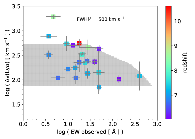
Figure 1: The Ly$\alpha$ observables of our sample. $\Delta v_{\mathrm{red}}(\mathrm{Ly}\alpha)$ is plotted on the ordinate axis, with EW on the abscissa. Galaxy redshift is color-coded, with the colorbar to the right. The shaded region shows the parameter space that can be matched using the emergent line profile of a low-$z$ galaxy (Hayes et al., 2023), when broadened synthetically to FWHM $=500$ km s^-1. We assume the IGM density at $z=7$, vary the velocity from 0 to 3000 km s^-1, and the EW between 0 and the very high value of 800 Å.

We obtain the spectral measurements for 23 galaxies at $z>6$, by combining various literature samples. We include the fifteen galaxies compiled by Endsley et al. (2022b), searching the primary references to obtain uncertainties on the Ly$\alpha$ EW and its velocity offset, $\Delta v_{\mathrm{red}}(\mathrm{Ly}\alpha)$. We add eight more galaxies with recently-obtained measurements from JWST. Six of these are taken from the The Cosmic Evolution Early Release Science Survey (CEERS, Finkelstein et al., 2023) that have Ly$\alpha$ detections: four from Tang et al. (2023) at $z=7.4-8.7$, and two from Jung et al. (2023) at $z\simeq 7.5$ after excluding one system for which $z_{\mathrm{sys}}$ is discussed as uncertain. The final two targets are JADES targets GNz11 at $z\simeq 10.6$ (Bunker et al., 2023) and GS-z7-LA at $z\simeq 7.3$ (Saxena et al., 2023). The main properties of interest are Ly$\alpha$ EW, velocity offset of the red peak, systemic redshifts and UV magnitudes. We show the distribution of these properties in Figure 1.

We note that this is a compilation of sources reported in different surveys, and requires spectroscopic detections in both Ly$\alpha$ and non-resonant emission lines. The quantitative interpretation will naturally be prone to selection effects. For example, over such a broad redshift range Malmquist biases are possible, but within this small sample there is currently no systematic evolution in the average luminosity. Different emission lines also measure $z_{\mathrm{sys}}$ at different redshifts, potentially impacting redshift precision where only weak lines are visible, but these uncertainties are treated within our method (Section 3.3). There is a general trend for galaxies with larger velocity shifts to show smaller EWs: this trend has been noted before, and is demonstrated in low-$z$ samples (e.g. Hayes et al., 2023) where the IGM has no influence. The relation probably arises because more massive galaxies have higher column densities of neutral gas: Ly$\alpha$ photons must therefore undergo more scattering events in order to take longer frequency excursions to the wings of the line profile and see the gas as optically thin (e.g. Verhamme et al., 2008; Hashimoto et al., 2013). This results in larger velocity offsets and also smaller Ly$\alpha$ escape fractions, because of the increased probability of dust absorption.

As the IGM becomes thicker with increasing redshift, and ionized regions are presumably smaller, a trend of increasing $\Delta v_{\mathrm{red}}(\mathrm{Ly}\alpha)$ with redshift could be expected. However, the apparent trend for galaxies with larger velocity shifts to lie at $z\gtrsim 7.5$ is not found to be significant by a two-sample Kolmogorov-Smirnoff test.

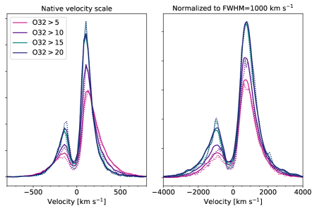
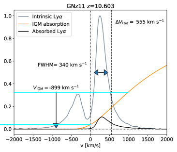
Figure 2: Left: model Ly$\alpha$ profiles. The far left spectrum shows the stacked profiles, where each spectrum is simply renormalized in luminosity at $\Delta v>0$ before stacking. As illustration, each colored line shows the stack of a subsample where all galaxies exceed the labeled O₃₂ ratio: greater than 5 in pink to greater than 20 in black. The central spectrum shows the same as the left, but the spectra are also rescaled to the same FWHM of the red peak prior to stacking. The reference FWHM is set to 1000 km s^-1 (note the different abscissa range of the two plots). Solid lines are mean stacks and dotted lines are median. The far right panel shows an example profile for GNz11 before and after IGM attenuation. We show the emergent Ly$\alpha$ profile as the grey line and the shape of the best-recovered Gunn Peterson absorption in orange. The observed Ly$\alpha$ profile is the product of the two and is shown in black. Various characteristic velocities are labeled.

3 Modeling Galaxies at Redshift 6–11

3.1 The ‘Emergent’ Lyman alpha profile

We use three different adjectives to describe Ly$\alpha$ in this paper: the intrinsic properties that are produced by the H ii regions, and the observed properties that reach the telescope are commonly-used terms. Here we also use the term emergent, which refers to the Ly$\alpha$ emitted by the galaxy (after the CGM) but before attenuation by the IGM. The emergent Ly$\alpha$ profile is estimated from the sample of starburst galaxies at $0.05<z<0.44$ observed with the Cosmic Origins Spectrograph on HST (Hayes et al., 2021, 2023). At this redshift, the Ly$\alpha$ profile is unaffected by IGM absorption.

In Hayes et al. (2023) we produced stacked average Ly$\alpha$ spectra, where we binned the sample by various galaxy properties. Here we use the same software to estimate the emergent Ly$\alpha$ profiles from the EoR galaxies, and show some examples in the left panels of Figure 2. We stack spectra based up measured quantities that match galaxies recently observed with JWST/NIRspec (e.g. Brinchmann, 2022; Cameron et al., 2023; Tang et al., 2023), such as high [O iii]$\lambda 5007$/[O ii]$\lambda 3727$ line ratios ($\equiv\mathrm{O}_{32}$). We adopt the stack of galaxies with $\mathrm{O}_{32}$ ratios above 10, to approximately match the measured values at $z>6$ where these measurements have been made (Tang et al., 2023; Saxena et al., 2023). While the optical spectroscopic properties of the low- and high-$z$ galaxies match well, the study relies upon invariance of the Ly$\alpha$ profiles with redshift, which we cannot test directly for EoR galaxies. However we showed in Hayes et al. (2021) that these profiles accurately reproduce those of Ly$\alpha$-emitters at $3\lesssim z\lesssim 6$ when the effects of an absorbing IGM are applied. We regard this as cause for optimism, and assert that the same general profile shape can be applied at higher redshifts still.

All spectra are first continuum-subtracted, using the modeled continuum spectra described in Hayes et al. (2023) and Hayes (2023). We then shift all spectra into the restframe, using the systemic redshifts measured from optical emission lines – average stacks of these spectra are shown in the left panel of Figure 2, where each has been normalized by the luminosity in the red Ly$\alpha$ peak before combination. However, because we are mostly interested in the spectral shape of the Ly$\alpha$ profile at velocities redwards of line-centre, we also re-normalize our spectra onto a common frequency metric: we convert the spectra to velocity space, and rescale each to FWHM=1000 km s^-1 in the red peak – these are shown in the central panel of Figure 2. The individual resampled spectra are renomalized by redshifted Ly$\alpha$ luminosity before combination. This provides us with the average shape of the Ly$\alpha$ emission, and in computing it we have written up a function to give the Ly$\alpha$ profile for an arbitrary input FWHM. Thus, our software treats FWHM as a free parameter.

3.2 Absorption by the Intergalactic Medium

With a model for the emergent Ly$\alpha$ profiles, we attenuate the spectra with a model IGM. We take the cosmic hydrogen number density scaled by a factor of $(1+z_{\mathrm{sys}})^{3}$ at each redshift. From this we calculate the expected Ly$\alpha$ optical depth profile $\tau_{\mathrm{IGM}}(v)$ as a function of velocity, as radiation redshifts through a neutral universe.

The unknown quantity is by how much the Ly$\alpha$ is cosmologically redshifted before it encounters the absorbing H i in the foreground. We estimate the absorption of Ly$\alpha$ using Voigt profiles, implementing successive absorptions numerically over velocity shift, $\Delta v_{\mathrm{IGM}}$, which equates to a distance in an expanding universe. We multiply the emergent Ly$\alpha$ profile by $\exp(-\tau_{\mathrm{IGM}}(v))$ and calculate the zeroth and first moments of the ‘observed’ profile. For a given emergent EW we rescale the zeroth moment to an ‘observed’ EW that accounts for the IGM. I.e $EW_{\mathrm{obs}}=EW_{\mathrm{emerge}}(m_{\mathrm{0,obs}}/m_{\mathrm{0,emerge}})$. $EW_{\mathrm{emerge}}$ therefore becomes a free parameter in our model, and can be compared with the EWs and velocity shifts shown in Figure 1.

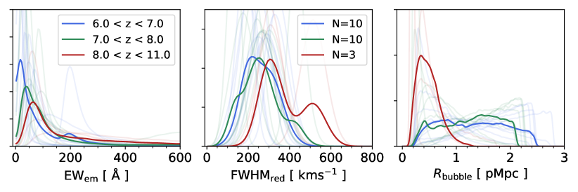
Figure 3: Binned probability distribution functions from traces of the Monte Carlo sampler. Left shows the emergent Ly$\alpha$ EW, and center shows the FWHM of the Ly$\alpha$ red peak. Right shows the bubble size in proper Mpc. Each posterior is color-coded by redshift, as labeled in the left plot. Hard lines show the means of the posterior distributions in each redshift bin, while faint lines show those for individual galaxies. The number of galaxies per bin is shown in the legend of the central plot.

3.3 Bayesian Inference on EW_em, FWHM_red, and $R_{\mathrm{B}}$

For each galaxy, we perform a hierarchical Bayesian inference analysis to estimate the free parameters of our model: $EW_{\rm em}$, $FWHM_{\rm red}$, and $R_{\mathrm{B}}$. We model the likelihood of observing the available data, i.e., the pair of $\{EW_{\mathrm{obs}}\pm\sigma_{EW_{\mathrm{obs}}},\Delta(v_{\mathrm{Ly\alpha}})_{\mathrm{obs}}\pm\sigma_{\Delta(v_{\mathrm{Ly\alpha}})}\}$, with a bivariate Normal distribution including known errors. Defining the vector of model parameters as $\theta=\{EW_{\rm em},FWHM_{\rm red},v_{\rm IGM}\}$, we write the posterior for $\theta$ as:

$$p(\theta|EW_{\mathrm{obs}},\sigma_{EW_{\mathrm{obs}}},\Delta(v_{\mathrm{Ly\alpha}})_{\mathrm{obs}},\sigma_{\Delta(v_{\mathrm{Ly\alpha}})},M_{\mathrm{UV}})\propto\\ N(EW_{\mathrm{tr}},\Delta(v_{\mathrm{Ly\alpha}})_{\mathrm{tr}}|\sigma_{EW_{\mathrm{obs}}},\sigma_{\Delta(v_{\mathrm{Ly\alpha}})},\theta,M_{\mathrm{UV}})p(\theta|M_{\mathrm{UV}})$$

where $p(\theta|M_{UV})$ is the prior on the model parameters, given the UV magnitude of each galaxy. Subscript ‘tr’ refers to Ly$\alpha$ quantities after transmission through the IGM, which are compared to the observed quantities given a subscript ‘obs’. We assume that $p(\theta|M_{\mathrm{UV}})=p(EW_{\mathrm{em}})p(v_{\rm IGM})p(FWHM_{\rm red}|M_{\mathrm{UV}})$, i.e., the priors on the emergent EW, the Ly$\alpha$ line width and the bubble radius are independent. The prior on $\Delta v_{\mathrm{IGM}}$ is the simplest to treat – we have no empirical knowledge of this and adopt a uniform prior. For the emergent FWHM distribution we base our prior upon strong trends between $M_{\mathrm{UV}}$ and the FWHM of the red peak (Hayes et al., 2023). We adopt measurements from the Lyman alpha Spectral Database (LASD; Runnholm et al., 2021) and the GALEX-measured UV magnitudes (see Hayes et al., 2023, Figure 21 of the online-only material) and fit a power-law between FWHM and $M_{\mathrm{UV}}$; our prior is then Normal around this relation, and includes errors on the fit. For the emergent Ly$\alpha$ EW we adopt an exponential distribution based upon very deep MUSE and HST observations at $z=6$. We take the exponential scale length of $EW_{0}=212\pm 186$Å from Hashimoto et al. (2017). This value is already corrected for IGM absorption in that paper (following Inoue et al. 2014, same as Hayes et al. 2021), and thus should be comparable to the emergent EW required for our method. We then make the assumption that the EW distribution does not evolve strongly over the redshift of the sample.

We sample the posterior distribution using a Metropolis Hastings sampler built in pycm (Salvatier et al., 2016). $\Delta v_{\mathrm{IGM}}$ is converted to $R_{\mathrm{B}}$ using Hubble’s law. We show an example fit in the right panel of Figure 2. In Figure 3 we show the posterior distribution functions for $EW_{\rm em}$, $FWHM_{\rm red}$, and $R_{\mathrm{B}}$ for each galaxy (light curves), divided into three samples according to redshift. In the discussion that follows, we use the maximum a posteriori and its associated 68% credibility interval as our best estimate and associated uncertainty on each parameter.

4 Main Results and Discussion

4.1 An Example: GNz11

We show an example model for GNz11 (Bunker et al., 2023) in the right panel of Figure 2. This is currently the highest redshift known Ly$\alpha$-emitting galaxy. The galaxy has an observed Ly$\alpha$ EW of 18 Å, and $\Delta v_{\mathrm{red}}(\mathrm{Ly}\alpha)$ of 555 km s^-1. While it may be an AGN, our models show that its spectral properties in Ly$\alpha$ can be recovered with relatively normal conditions. Naively, it may be considered difficult to explain a Ly$\alpha$ emission line from $z=10.6$, but in actuality it is not especially hard.

The maximum of the posterior on the Ly$\alpha$ FWHM is 340 km s^-1 – this is quite high, but within the range of widths measuerd in low-$z$ galaxies (the broadest we find in the $z\sim 0$ COS sample has a FWHM=350 km s^-1 in its red peak). This modeled broad Ly$\alpha$ has a wing visible out to $v\simeq 1200$ km s^-1 at low flux density. The maximum of the posterior probability function for the IGM velocity is almost 900 km s^-1 – at this velocity offset, the damping wing draws a steep diagonal line across the emerging red Ly$\alpha$ peak, absorbing $\sim 8$ times more flux at $v=0$ compared to at $v=1000$ km s^-1. The result is a significant shift in the first moment of the line, to the 555 km s^-1 that is observed. In doing so the Ly$\alpha$ is also significantly suppressed, and only $\sim 7$% of the emergent Ly$\alpha$ survives IGM absorption. The emergent Ly$\alpha$ EW is $\simeq 260$ Å with a credibility range of 153–800 Å at 16–84%. This value is again high for a star-forming galaxy, but not higher than observed in galaxies at effectively all redshifts. Based upon the observed H$\gamma$ flux and Case B recombination theory, Bunker et al. (2023) estimate that around 4% of the intrinsic Ly$\alpha$ escapes the galaxy. The is comparable to the 7 % we estimate from the emergent Ly$\alpha$ flux; the further factor of $\sim 2$ could indicate that $\sim 50$ % of the intrinsic Ly$\alpha$ escapes the galaxy after internal radiative transfer effects.

4.2 Sample-Averaged Galaxy Properties

We take the H i velocity offsets, emergent Ly$\alpha$ EW and FWHM from the maximum values of the posterior sampling (Section 3.3) and show the pdfs in Figure 3. Faint lines show the pdfs for individual galaxies, color coded by redshift, while solid lines show the arithmetic mean pdf in each bin. Emergent EWs are typically peaked towards the lower end of the distribution near 100 Å – a value that is quite typical of star-forming galaxies and does not require extreme stellar populations or AGN. Only a handful of individual galaxies show posteriors that peak at EWs above 200 Å, one of which is obviously JADES-GS-z7-LA, with its observed EW of 400 Å.

The FWHM also peak in ranges that are typical of star forming galaxies at low-$z$, of around 200 km s^-1, with a tail up to 600 km s^-1. Here there is a more obvious signature for galaxies at the higher redshifts to be intrinsically broader than those at $z=6-8.5$, although we note that this highest redshift bin contains only three galaxies. This may be a signature of a selection bias in the requirement of Ly$\alpha$, where only broad emergent Ly$\alpha$ profiles are able evade the damping wing of the IGM and be reported as a Ly$\alpha$ detection.

4.3 The Evolution of Ionized Regions Through the EoR

After converting the IGM velocity offset to a foreground H i distance using the Hubble parameter, we show the resulting combined posterior probabilities in the right panel of Figure 3. Estimated H i foreground distances generally show flat combined posteriors for the $z=6-8$ subsamples, which indicates a broad range of bubble sizes, from $\simeq 0.5$ pMpc, and extending to $\simeq 2.5$ Mpc. However the combined posterior of the $z>8$ subsample is much more strongly peaked around distances below 1 pMpc, shows a much sharper decline with redshift, and drops to zero at 1 pMpc.

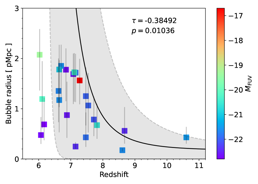
Figure 4: Evolution of the bubble radius, $R_{\mathrm{B}}$ (ordinate) with redshift (abscissa). Uncertainties refer to the 16th and 84th percentiles of the posterior. Absolute UV magnitude is color-coded. The shaded regions shows the 10-90-percentile range of bubble sizes from the simulation of Giri & Mellema (2021).

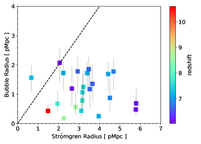
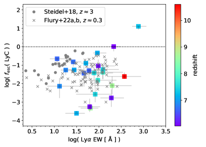
Figure 5: Left: the radii of the bubble inferred from Ly$\alpha$ modeling ($R_{\mathrm{B}}$), contrasted with that of the Strömgren sphere ($R_{\mathrm{S}}$). Right: the comparison of the LyC escape fraction ($f_{\mathrm{esc}}^{\mathrm{LyC}}$; inferred from the left plot) with the model-inferred EW of Ly$\alpha$. We over-plot the values measured at $z\simeq 3$ by Steidel et al. (2018) and at $z\simeq 0.3$ by Flury et al. (2022a). Redshift is color-coded in both cases.

In Figure 4 we show the evolution of the distance to the foreground screen of H i (taking the peak of the posterior) as a function of redshift. Distances to the foreground H i screen range from around 0.5 to 2.5 proper Mpc at the lower redshift end. We note that our approach – and observations in general – may not be sensitive to smaller bubble radii, as a certain minimum offset will be required for Ly$\alpha$ to be detected, and therefore be reported in the literature. There is in principle no reason why the method could not be applied to galaxies without Ly$\alpha$ emission, but in order to avoid great degeneracies such an approach would require more informed priors on the intrinsic EW. This could perhaps be attained from optical line emission (e.g. Runnholm et al., 2020; Hayes et al., 2023).

The interpretation of the larger radii at $z\simeq 6$ is likely to be that the these galaxies reside in an ionized universe, and far out in the damping wing (after $\sim 2000$ km s^-1) there is little power in the IGM to modulate the Ly$\alpha$ observables – the method breaks down for large bubbles and all $\Delta v_{\mathrm{IGM}}$ are equally valid. The lower end of the distribution ($\Delta v_{\mathrm{IGM}}$ $\simeq 1$ pMpc) are consistent estimates from Ly$\alpha$ spectral profiles (Mason & Gronke, 2020) and from ionization balance considerations (Bagley et al., 2017), both of which are estimated at comparable redshifts.

Figure 4 is striking in its absence of larger bubbles at higher redshifts. Using Kendall’s $\tau$ statistic, we find the trend to be significant at $p=1\times 10^{-2}$, and we note that similar credibility regions are determined at $z>8$ compared with the galaxies at the lower redshift end of the sample. If taken at face value, the result implies that ionized regions increase in size from $z\simeq 11$ to 6 – this empirical find of ionized regions growing with time fulfills the main expectations of reioinization. The selection bias of needing Ly$\alpha$ in emission may also enter here: smaller bubbles will not enable Ly$\alpha$ transfer through the IGM, implying a lower limit on the bubble sizes we can capture. As this is more likely to be the case at earlier times, the strength of the relationship would only increase.

In the same figure we also show computational results from Giri & Mellema (2021). The simulated relation takes a similar form: starting from $z\sim 11$, the bubble size of GNz11 falls just at the upper edge of the distribution. The simulated bubble sizes then increases towards $z\simeq 7$, forming a fully ionized universe (effectively infinite bubble radii) by $z=6.5$. However, simulated bubbles grow somewhat faster than our data suggest. There are four observed galaxies at $z\sim 6$ that seemingly have much smaller bubble radii than suggested by the simulations. If the universe is fully ionized at $z=6$ on these sightlines, the inference for these galaxies could be the result of proximate Ly$\alpha$-absorbing systems (possibly galaxies) whose damping wings suppress and redshift Ly$\alpha$, and cause our model estimate smaller radii. This result may reflect the high end of the broader range of Ly$\alpha$ optical depths observed in quasar spectra at $z\approx 6$ (e.g. Bosman et al., 2022).

4.4 The Escape of Ionizing Radiation

In Section 4.3 we estimated the distance between the galaxy and the absorbing H i gas in the foreground. Here we test whether these main targeted galaxies are capable of ionizing their own H ii regions and, if so, what their properties must be. We proceed by simply investigating the size of the Strömgren sphere: $R_{\mathrm{S}}$ $=(3Q_{0}f_{\mathrm{esc}}^{\mathrm{LyC}}/4\pi n_{\mathrm{H}}^{2}\alpha_{\mathrm{B}})^{1/3}$. Here, $Q_{0}$ is the intrinsic production rate of ionizing photons and $f_{\mathrm{esc}}^{\mathrm{LyC}}$ is the ionizing escape fraction; hence the product of the two is the emitted ionizing photon rate. $\alpha_{\mathrm{B}}$ is the (temperature dependent) total recombination rate coefficient under Case B, for which we assume $10^{4}$ K. This includes three main assumptions: (1.) that we can estimate $Q_{0}$ from data; (2.) that galaxies remain ionizing for long enough to ionize their surrounding media; (3.) the IGM is homogeneous and of fixed density.

We assume $n_{\mathrm{H}}$ to be the cosmic value at the redshift of each galaxy, as we described also for the inference in Section 3.2. Each galaxy must be strongly star-forming, as evidenced by the emergent Ly$\alpha$ EWs of 100 Å (intrinsic values are likely higher still). Addressing assumption 1 above, we assume the ionizing photon production efficiency ($\xi_{\mathrm{ion}}$) measured for GNz11 of $5.2\times 10^{25}$ Hz erg^-1 (Bunker et al., 2023) and convert the UV luminosity to $Q_{0}$. By first setting $f_{\mathrm{esc}}^{\mathrm{LyC}}$ to 1, we compute $R_{\mathrm{S}}^{\mathrm{max}}$, finding values between 0.5 and 6 Mpc. We contrast this with the distances to the foreground H i (0.5–2.5 pMpc) in the left panel of Figure 5. It is immediately obvious that, if the above assumptions hold, then 22 of the 23 galaxies have sufficient ionizing power to ionize their own bubble.

Obviously $f_{\mathrm{esc}}^{\mathrm{LyC}}$ cannot be 1, or the galaxies would not produce the strong Ly$\alpha$ or observed nebular line emission. $f_{\mathrm{esc}}^{\mathrm{LyC}}$ cannot be measured at these redshifts, but under the assumption that each galaxy is singularly responsible for ionizing its own H ii region, we can solve for $f_{\mathrm{esc}}^{\mathrm{LyC}}$ in each galaxy by setting $R_{\mathrm{S}}$ equal to the inferred bubble size: $f_{\mathrm{esc}}^{\mathrm{LyC}}=(R_{\mathrm{Bub}}/R_{\mathrm{S}})^{3}$. We show $f_{\mathrm{esc}}^{\mathrm{LyC}}$ against the inferred Ly$\alpha$ EW in the right panel of Figure 5. These two quantities are strongly correlated at low- and mid-redshifts and we overplot the individual data points of Flury et al. (2022b) and stacks and Steidel et al. (2018) for comparison. Our estimates span the same range as the lower redshift estimates. While this plot is suggestive that relationship could also be identifiable for galaxies in the EoR, we do not yet have sufficient samples to make similar statements. The median value of $f_{\mathrm{esc}}^{\mathrm{LyC}}$ in our sample is 5.1 %, with a 16–84 percentile range of 1–21%, which is broadly consistent with requirements for cosmic reionization (e.g. Finkelstein et al., 2019). For GNz11 we estimate $f_{\mathrm{esc}}^{\mathrm{LyC}}$ to be just 2.4 % with a $1\sigma$ confidence intervals between 1 and 6.1%. This is remarkably coincident with the value of $0.03^{+0.05}_{-0.02}$, estimated by Bunker et al. (2023) using completely different methods. One galaxy significantly outlies the distribution, with $R_{\mathrm{B}}$ almost 3 times its supposed Strömgren radius, leading to an apparent escape fraction of 13. This is the extreme galaxy GS-z7-LA (Saxena et al., 2023), with Ly$\alpha$ EW of 400Å, and demonstrating that our assumptions do not hold everywhere.

5 Sources of Uncertainty

We now discuss each of the assumptions above as a source of uncertainty, beginning with the ionizing photon production efficiency. We have assumed log($\xi_{\mathrm{ion}}$/Hz erg^-1) $=25.7$ throughout. In our formulation $f_{\mathrm{esc}}^{\mathrm{LyC}}$ $\propto\xi_{\mathrm{ion}}^{-1}$, and variations of a factor of 2 in $\xi_{\mathrm{ion}}$ will change $f_{\mathrm{esc}}^{\mathrm{LyC}}$ by the corresponding amount. Significant reductions in $\xi_{\mathrm{ion}}$ are hard to envisage, as they must be able to reproduce the strong emergent Ly$\alpha$ and nebular line emission observed in the available JWST spectra. Increasing $\xi_{\mathrm{ion}}$ by a factor of 2 may perhaps be possible (e.g. Maseda et al., 2020), but values higher than this would become inconsistent with predictions from normal stellar populations.

Secondly we have assumed the Strömgren sphere can fully form, which would require $\simeq 0.6-7$ Myr based upon the inferred range of $R_{\mathrm{B}}$, and is largest at the lower redshift end. This timescale is short compared to the typical ionizing timescales of galaxies, even at this epoch. By modeling the SEDs of galaxies at a similar epoch, (Endsley et al., 2022a) find typical stellar ages greater than this for $\simeq 80$ % of their sample (and also exactly the same median value of $\xi_{\mathrm{ion}}$ we adopt above). Moreover, starburst events should not coordinate on times shorter than the freefall timescale, $t_{\mathrm{ff}}$: to bring $t_{\mathrm{ff}}$ below 7 Myr for a mass of $10^{8}$ M_⊙ would require all gas to fall from a radius of just 250 pc, which we deem unrealistic.

Next we address the assumption of fixed $n_{\mathrm{H}}$: $f_{\mathrm{esc}}^{\mathrm{LyC}}$ is proportional to the square of this density. It is worth noting that recombination timescale of gas at cosmic $n_{\mathrm{H}}$ is about twice the Hubble time at $z=6$: global recombinations do not significantly affect our calculations. If $n_{\mathrm{H}}$ varies substantially, it will also impact our estimates of $R_{\mathrm{B}}$, and to test this we have re-run our inference with $n_{\mathrm{H}}$ rescaled from the cosmic average. Reducing $n_{\mathrm{H}}$ by a factor of 2 decreases the median $R_{\mathrm{B}}$ by only 16%, but increases $R_{\mathrm{S}}$ by 60%; consequently $f_{\mathrm{esc}}^{\mathrm{LyC}}$ decreases to a median value of $\simeq 1$%. However it is very unlikely that the vicinity of galaxies is underdense at all compared to the cosmic average. The reverse situation is more likely: doubling $n_{\mathrm{H}}$ marginally increases $R_{\mathrm{B}}$, while $R_{\mathrm{S}}$ decreases, causing the median $f_{\mathrm{esc}}^{\mathrm{LyC}}$ to increase to $\simeq 18$%, which remains a realistic value in the EoR. In the instance where gas is clumped on smaller scales within the bubble, dense regions will experience increased recombination rates while the regions between them will have lower densities, which allows ionization fronts to propagate faster. In this case, sightline effects could also become important: if the denser regions lie in front of a galaxy, the excess absorption will push the inferred $R_{\mathrm{B}}$ to larger values to compensate. Assuming the denser clumps occupy a small volume, the decreased $n_{\mathrm{H}}$ elsewhere will mean the true $R_{\mathrm{S}}$ is slightly larger than our estimate. In this instance $f_{\mathrm{esc}}^{\mathrm{LyC}}$ will be underestimated, although if the denser regions lie outside of our sightline, the effects will mostly cancel.

Finally, we address the question of multiple galaxies contributing to the ionization of a single H ii region, which is indeed likely. However, it is also probable that the UV-selection of these targets has found the most luminous galaxy in the vicinity. Our median value of $R_{\mathrm{B}}$ $=1.1$ physical Mpc corresponds to a volume of $\simeq 2850$ comoving Mpc³ at $z=7$, and such a volume would on average contain only 0.04 galaxies brighter than $L^{\star}$ according to the recent LF of Harikane et al. (2023). In an unclustered universe, we would have to integrate to luminosities $\sim 5$ times fainter for the probability of finding another galaxy within $R_{\mathrm{B}}$ to reach 1. With all other quantities held constant, this would add only 20% more ionizing luminosity and not substantially changing the results. Of course galaxies do cluster, but we expect these results to hold on average in cases where the most luminous local source has been identified. We expect, however, that this is not the case for the very faint galaxy GS-z7-LA (Saxena et al., 2023), which has an observed Ly$\alpha$ EW of $\simeq 400$Å, and almost certainly requires assistance from nearby ionizing sources.

6 Concluding Remarks

We have built a hierarchical Bayesian model to estimate the intrinsic Ly$\alpha$ observables (emergent equivalent width and kinematic offset from systemic velocity) of galaxies in the reionization epoch, as well as the size of the ionized regions (‘bubbles’) in which they must reside. The model is built upon empirical Ly$\alpha$ spectral templates observed in lower redshift galaxies where the IGM has no impact, and estimates the IGM absorption at a given redshift that best matches observation. We have applied this framework to a sample of 23 ostensibly star-forming galaxies at redshift $z=6-11$ where systemic redshifts are available, including very recent observations from JWST. We find the following main results.

• The observed galaxies occupy ionized regions with sizes between 0.5 and 2.5 proper Mpc. The posterior probability distribution of the bubble size is not invariant with redshift, and is skewed towards smaller bubbles at higher redshifts. We detect an upwards evolution of the bubble size with redshift that is significant at better than $3\sigma$ and demonstrates that ionized regions grow with time. The recovered bubble radii are broadly consistent with results from numerical simulations of reionization.

• From the observed UV luminosity and reported ionizing photon production efficiencies, we compute the size of the Strömgren radius of each galaxy. The Strömgren radius does not correlate with the bubble radius. We use the ratio of these two radii to estimate the escape fraction of ionizing photons, recovering a median value of 5% – this is marginally consistent with the requirements for galaxies to reionize the universe. If the IGM density within the ionized region is overdense by a factor of 2, $f_{\mathrm{esc}}^{\mathrm{LyC}}$ increases to 18%. Our estimates of $f_{\mathrm{esc}}^{\mathrm{LyC}}$ and Ly$\alpha$ EW are comparable to those derived at lower-$z$, but we do not yet recover the correlation between these quantities.

References

- Arrabal Haro et al. (2018) Arrabal Haro, P., Rodríguez Espinosa, J. M., Muñoz-Tuñón, C., et al. 2018, MNRAS, 478, 3740, doi: 10.1093/mnras/sty1106
- Bagley et al. (2017) Bagley, M. B., Scarlata, C., Henry, A., et al. 2017, ApJ, 837, 11, doi: 10.3847/1538-4357/837/1/11
- Bosman et al. (2022) Bosman, S. E. I., Davies, F. B., Becker, G. D., et al. 2022, MNRAS, 514, 55, doi: 10.1093/mnras/stac1046
- Brinchmann (2022) Brinchmann, J. 2022, arXiv e-prints, arXiv:2208.07467, doi: 10.48550/arXiv.2208.07467
- Bunker et al. (2023) Bunker, A. J., Saxena, A., Cameron, A. J., et al. 2023, arXiv e-prints, arXiv:2302.07256, doi: 10.48550/arXiv.2302.07256
- Cameron et al. (2023) Cameron, A. J., Saxena, A., Bunker, A. J., et al. 2023, arXiv e-prints, arXiv:2302.04298, doi: 10.48550/arXiv.2302.04298
- Carniani et al. (2017) Carniani, S., Maiolino, R., Pallottini, A., et al. 2017, A&A, 605, A42, doi: 10.1051/0004-6361/201630366
- Cassata et al. (2015) Cassata, P., Tasca, L. A. M., Le Fèvre, O., et al. 2015, A&A, 573, A24, doi: 10.1051/0004-6361/201423824
- Dijkstra (2014) Dijkstra, M. 2014, PASA, 31, e040, doi: 10.1017/pasa.2014.33
- Dijkstra et al. (2006) Dijkstra, M., Haiman, Z., & Spaans, M. 2006, ApJ, 649, 14, doi: 10.1086/506243
- Dijkstra et al. (2007) Dijkstra, M., Wyithe, J. S. B., & Haiman, Z. 2007, MNRAS, 379, 253, doi: 10.1111/j.1365-2966.2007.11936.x
- Endsley et al. (2022a) Endsley, R., Stark, D. P., Whitler, L., et al. 2022a, arXiv e-prints, arXiv:2208.14999, doi: 10.48550/arXiv.2208.14999
- Endsley et al. (2022b) Endsley, R., Stark, D. P., Bouwens, R. J., et al. 2022b, MNRAS, 517, 5642, doi: 10.1093/mnras/stac3064
- Finkelstein et al. (2019) Finkelstein, S. L., D’Aloisio, A., Paardekooper, J.-P., et al. 2019, ApJ, 879, 36, doi: 10.3847/1538-4357/ab1ea8
- Finkelstein et al. (2023) Finkelstein, S. L., Bagley, M. B., Ferguson, H. C., et al. 2023, ApJ, 946, L13, doi: 10.3847/2041-8213/acade4
- Flury et al. (2022a) Flury, S. R., Jaskot, A. E., Ferguson, H. C., et al. 2022a, ApJS, 260, 1, doi: 10.3847/1538-4365/ac5331
- Flury et al. (2022b) —. 2022b, ApJ, 930, 126, doi: 10.3847/1538-4357/ac61e4
- Giri & Mellema (2021) Giri, S. K., & Mellema, G. 2021, MNRAS, 505, 1863, doi: 10.1093/mnras/stab1320
- Harikane et al. (2023) Harikane, Y., Ouchi, M., Oguri, M., et al. 2023, ApJS, 265, 5, doi: 10.3847/1538-4365/acaaa9
- Hashimoto et al. (2013) Hashimoto, T., Ouchi, M., Shimasaku, K., et al. 2013, ApJ, 765, 70, doi: 10.1088/0004-637X/765/1/70
- Hashimoto et al. (2017) Hashimoto, T., Garel, T., Guiderdoni, B., et al. 2017, A&A, 608, A10, doi: 10.1051/0004-6361/201731579
- Hayes et al. (2011) Hayes, M., Schaerer, D., Östlin, G., et al. 2011, ApJ, 730, 8, doi: 10.1088/0004-637X/730/1/8
- Hayes (2023) Hayes, M. J. 2023, MNRAS, 519, L26, doi: 10.1093/mnrasl/slac135
- Hayes et al. (2021) Hayes, M. J., Runnholm, A., Gronke, M., & Scarlata, C. 2021, ApJ, 908, 36, doi: 10.3847/1538-4357/abd246
- Hayes et al. (2023) Hayes, M. J., Runnholm, A., Scarlata, C., Gronke, M., & Rivera-Thorsen, T. E. 2023, MNRAS, 520, 5903, doi: 10.1093/mnras/stad477
- Inoue et al. (2014) Inoue, A. K., Shimizu, I., Iwata, I., & Tanaka, M. 2014, MNRAS, 442, 1805, doi: 10.1093/mnras/stu936
- Jung et al. (2023) Jung, I., Finkelstein, S. L., Arrabal Haro, P., et al. 2023, arXiv e-prints, arXiv:2304.05385, doi: 10.48550/arXiv.2304.05385
- Kashikawa et al. (2006) Kashikawa, N., Shimasaku, K., Malkan, M. A., et al. 2006, ApJ, 648, 7, doi: 10.1086/504966
- Laursen et al. (2009) Laursen, P., Sommer-Larsen, J., & Andersen, A. C. 2009, ApJ, 704, 1640, doi: 10.1088/0004-637X/704/2/1640
- Mainali et al. (2017) Mainali, R., Kollmeier, J. A., Stark, D. P., et al. 2017, ApJ, 836, L14, doi: 10.3847/2041-8213/836/1/L14
- Malhotra & Rhoads (2004) Malhotra, S., & Rhoads, J. E. 2004, ApJ, 617, L5, doi: 10.1086/427182
- Maseda et al. (2020) Maseda, M. V., Bacon, R., Lam, D., et al. 2020, MNRAS, 493, 5120, doi: 10.1093/mnras/staa622
- Mason & Gronke (2020) Mason, C. A., & Gronke, M. 2020, MNRAS, 499, 1395, doi: 10.1093/mnras/staa2910
- Mason et al. (2018) Mason, C. A., Treu, T., Dijkstra, M., et al. 2018, ApJ, 856, 2, doi: 10.3847/1538-4357/aab0a7
- Matthee et al. (2018) Matthee, J., Sobral, D., Gronke, M., et al. 2018, A&A, 619, A136, doi: 10.1051/0004-6361/201833528
- Miralda-Escudé & Rees (1998) Miralda-Escudé, J., & Rees, M. J. 1998, ApJ, 497, 21, doi: 10.1086/305458
- Pentericci et al. (2016) Pentericci, L., Carniani, S., Castellano, M., et al. 2016, ApJ, 829, L11, doi: 10.3847/2041-8205/829/1/L11
- Runnholm et al. (2021) Runnholm, A., Gronke, M., & Hayes, M. 2021, PASP, 133, 034507, doi: 10.1088/1538-3873/abe3ca
- Runnholm et al. (2020) Runnholm, A., Hayes, M., Melinder, J., et al. 2020, ApJ, 892, 48, doi: 10.3847/1538-4357/ab7a91
- Salvatier et al. (2016) Salvatier, J., Wiecki, T. V., & Fonnesbeck, C. 2016, PeerJ Computer Science, 2, e55, doi: 10.7717/peerj-cs.55
- Saxena et al. (2023) Saxena, A., Robertson, B. E., Bunker, A. J., et al. 2023, arXiv e-prints, arXiv:2302.12805, doi: 10.48550/arXiv.2302.12805
- Schenker et al. (2014) Schenker, M. A., Ellis, R. S., Konidaris, N. P., & Stark, D. P. 2014, ApJ, 795, 20, doi: 10.1088/0004-637X/795/1/20
- Stark et al. (2011) Stark, D. P., Ellis, R. S., & Ouchi, M. 2011, ApJ, 728, L2, doi: 10.1088/2041-8205/728/1/L2
- Stark et al. (2015) Stark, D. P., Richard, J., Charlot, S., et al. 2015, MNRAS, 450, 1846, doi: 10.1093/mnras/stv688
- Stark et al. (2017) Stark, D. P., Ellis, R. S., Charlot, S., et al. 2017, MNRAS, 464, 469, doi: 10.1093/mnras/stw2233
- Steidel et al. (2018) Steidel, C. C., Bogosavljević, M., Shapley, A. E., et al. 2018, ApJ, 869, 123, doi: 10.3847/1538-4357/aaed28
- Tang et al. (2023) Tang, M., Stark, D. P., Chen, Z., et al. 2023, arXiv e-prints, arXiv:2301.07072, doi: 10.48550/arXiv.2301.07072
- Verhamme et al. (2008) Verhamme, A., Schaerer, D., Atek, H., & Tapken, C. 2008, A&A, 491, 89, doi: 10.1051/0004-6361:200809648
- Verhamme et al. (2006) Verhamme, A., Schaerer, D., & Maselli, A. 2006, A&A, 460, 397, doi: 10.1051/0004-6361:20065554
- Wold et al. (2017) Wold, I. G. B., Finkelstein, S. L., Barger, A. J., Cowie, L. L., & Rosenwasser, B. 2017, ApJ, 848, 108, doi: 10.3847/1538-4357/aa8d6b