Abstract

Given a graph $G$, a subset $S$ of vertices of $G$ is an efficient dominating set (EDS) if $|N[v]\cap S|=1,$ for all $v\in V(G)$. A graph $G$ is efficiently dominatable if it possesses an EDS. The efficient domination number of $G$ is denoted by $F(G)$ and is defined to be $\max\left\{\sum_{v\in S}(1+\operatorname{deg}v):\right.$ $\left.S\subseteq V(G)\right.$ and $\left.|N[x]\cap S|\leq 1,\forall~{}x\in V(G)\right\}$. In general, not every graph is efficiently dominatable. Further, the class of efficiently dominatable graphs has not been completely characterized and the problem of determining whether or not a graph is efficiently dominatable is NP-Complete. Hence, interest is shown to study the efficient domination property for graphs under restricted conditions or special classes of graphs. In this paper, we study the notion of efficient domination in some Lattice graphs, namely, rectangular grid graphs ($P_{m}\Box P_{n}$), triangular grid graphs, and hexagonal grid graphs.

2010 Mathematics Subject Classification: 05C69,05B40

Keywords: Efficient domination, Efficient domination number, Independent perfect domination, $2$-packing, Lattice graphs, Grid graphs.

1 Introduction

Given a graph $G=(V,E)$, a set $S\subseteq V(G)$ is a dominating set if each vertex $v\in V(G)$ is either in $S$ or has at least one neighbor in $S$. The size of the smallest dominating set of $G$ is the domination number of $G$ and is denoted by $\gamma(G)$. The open neighborhood of a vertex $v$, denoted by $N(v)$, is the set of all vertices adjacent to $v$ and the closed neighborhood of $v$, denoted by $N[v]$ is defined as $N(v)\cup\{v\}$. A set $S\subseteq V(G)$ is an efficient dominating set (EDS) of $G$ if $|N[v]\cap S|=1$, for all $v\in V(G)$. That is, $S$ is an EDS, if each vertex $v\in V(G)$ is dominated by exactly one vertex (including itself) in $S$. Not every graph possesses an EDS. If a graph $G$ has an EDS, then it is said to be efficiently dominatable.

The distance between a pair of vertices $u$ and $v$ is the length of the shortest path between $u$ and $v$ and is denoted by $d(u,v)$. A set $S\subseteq V(G)$ is a 2-packing if for each pair $u,v\in S$, $N[u]\cap N[v]=\emptyset$. If $S$ is a 2-packing, then $d(u,v)\geq 3,$ for all $u,v\in S$. Thus, a dominating set is an EDS if and only if it is a $2$-packing. The influence of a set $S\subseteq V(G)$ is denoted by $I(S)$ and is the number of vertices dominated by $S$ (inclusive of vertices in $S$). If $S$ is a $2$-packing, then $I(S)=\sum_{v\in S}[1+\deg(v)].$ The maximum influence of a $2$-packing of $G$ is called the efficient domination number of $G$ and is denoted by $F(G)$. That is, $F(G)=\max\{I(S):~{}$S is a 2-packing$\}=\max\left\{\sum_{v\in S}(1+\operatorname{deg}v):S\subseteq V(G)\right.$ and $\left.|N[x]\cap S|\leq 1,\forall~{}x\in V(G)\right\}$. Clearly, $0\leq F(G)\leq|V(G)|$ and $G$ is efficiently dominatable if and only if $F(G)=|V(G)|$. A $2$-packing with influence $F(G)$ is called an $F(G)$-set.

The concept of efficient domination is found in the literature in different names like perfect codes or perfect $1$-codes [11], independent perfect domination [20], perfect $1$-domination [18] and efficient domination [2]. In this paper, we use the terminology “efficient domination” introduced by Bange et. al. [2]. The problem of determining whether $F(G)=|V(G)|$ is $\mathcal{NP}$-complete on arbitrary graphs [2] as well as on some special/restricted classes of graphs like bipartite graphs, chordal graphs, planar graphs of degree at most three, etc. [[15], whereas it is polynomial in the case of trees [2]. In [3], Goddard et al. have obtained bounds on the efficient domination number of arbitrary graphs and trees. Efficient Domination has also been studied on different special classes of graphs like chordal bipartite graphs [4], strong product of arbitrary graphs [5], cartesian product of cycles [12], etc. Hereditary efficiently dominatable graphs were defined and studied in [9] and [10].

The perfect codes or efficient domination finds wide applications in coding theory, resource allocation in computer networks, etc. (refer to [14], [17]), while lattice graph structures play a significant role in source and channel coding. Motivated by the applications and the graph theoretical significance of efficient domination and lattice structures, this papers focuses on the study of efficient domination in some special lattice structures, namely, finite rectangular grids ($P_{n}\Box P_{m}$, where $1\leq n,m<\infty$) (in 2.2.1), infinite rectangular grids (in 2.3.1), infinite triangular (in 2.3.2) and hexagonal grid graphs (in 2.3.3). The study on finite cases of triangular and hexagonal grid structures is in progress.

2 Main Results

2.1 Notations and Terminologies

Definition 2.1.

[16] The cartesian product of two graphs $G=(V_{1},\,E_{1})$ and $H=(V_{2},\,E_{2})$, denoted by $G\Box H$, is the graph with vertex set $V_{1}\times V_{2}$ in which two vertices $(u_{1},v_{1})$ and $(u_{2},\,v_{2})$ are adjacent if and only if either (i) $u_{1}=u_{2}$ and $v_{1}v_{2}\in E_{2}$ or (ii) $u_{1}u_{2}\in E_{1}$ and $v_{1}=v_{2}$.
The graphs $G$ and $H$ are called the factors of $G\Box H$. For $v\in V(H)$, the subgraph of $G\Box H$ induced by $\{(u,v)\in V(G\Box H):u\in V(G)\}$ is called the G-layer of $G\Box H$ with respect to $v$ and is denoted by $G^{(v)}$. Analogously, the $H$-layer, namely, $H^{(u)}$ is defined for each $u\in V(G).$

In literature, the cartesian product of two paths is referred by different terminologies like grid graphs, rectangular grid graphs, two-dimensional lattice graphs, etc. [13]. In this paper, we use rectangular grid graph to refer to the carterisan product of two paths $P_{n}$ and $P_{m}$.
In the discussions to follow, we consider three categories of rectangular grids:

• Those grids bounded on all four sides, referred to as finite rectangular grids, denoted by $P_{n}\Box P_{m}$, where $1\leq n,m<\infty$.

• Those grids bounded on three sides (top, left and right) or two sides (top and left) and unbounded on the other sides, denoted respectively as $\bf P_{n}\Box P_{\infty}$, where $\bf n\geq 1$ and $\bf P_{\infty}\Box P_{\infty}$.

• Those grids unbounded on all four sides, referred to as infinite rectangular grids.

Throughout this paper, we refer to vertices that are not dominated by a set as voids. In the figures given throughout this paper, shaded circular dots of larger size represent dominating vertices, shaded circular dots of smaller size denote vertices dominated by a set (excluding self-dominating vertices) and non-shaded circular dots correspond to voids.

2.2 Finite lattice graphs

2.2.1 Finite rectangular grid graphs

It is known that if a graph is efficiently dominatable, then all its EDSs are of same size and is equal to $\gamma(G)$ [1, 2]. The domination number of rectangular grid graphs has been studied in [6], [7]. In the discussions to follow, we give constructive characterizations for efficiently dominatable lattice graphs. In the case of graphs which are not efficiently dominatable, we obtain either the exact value or bounds of efficient domination number.

In what follows, assume that $V(P_{n}\Box P_{m})=\{v_{i,j}|1\leq i\leq m,1\leq j\leq n\}$, unless mentioned otherwise. For convenience, we label the $m$ $P_{n}$-layers of $P_{n}\Box P_{m}$ as $R_{1},R_{2},\dots R_{m}$ and its $n$ $P_{m}$-layers as $C_{1},C_{2},\dots C_{n}$, respectively. That is, for each $i$ $(1\leq i\leq m),$ $R_{i}\cong P_{n}$ and for each $j$ $(1\leq j\leq n),$ $C_{j}\cong P_{m}$. Further, it is noted that the distance between any two vertices $v_{i,j}$ and $v_{p,q}$ is $|i-p|+|j-q|$. With these conventions, the results discussed below lead to characterizations of efficiently dominatinable rectangular grids.

Theorem 2.2.

For $n\geq 1$, $P_{n}\Box P_{2}$ is efficiently dominatable if and only if $n$ is odd.

Proof.

The result is trivially true if $n=1$. So, assume that $n>1$ and $n$ is odd. That is, $n=2k+1$ for some natural number $k$. Then, $\{v_{1,j}|j=1,5,\dots,4\lfloor\frac{k}{2}\rfloor+1\}\cup\{(v_{2,j})|j=3,7,\dots,4\lfloor\frac{k-1}{2}\rfloor+3\}$ is an EDS of $P_{n}\Box P_{2}$ and hence, it is efficiently dominatable.

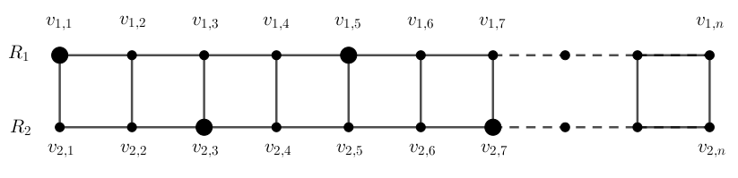
Figure 1: $P_{n}\Box P_{2}$

Suppose n is even, then we show that $F(P_{n}\Box P_{2})<2n.$ Let $n=2k$, for some natural number $k$ and $S$ be an $F(P_{n}\Box P_{2})$-set. If possible, assume that $I(S)=2n$. Then, by definition, $|N[v_{i,j}]\cap S|=1$, for each $v_{i,j}\in V(P_{n}\Box P_{2}).$

Consider an arbitrary vertex, say $v_{1,1}$. Since $I(S)=2n$, to dominate $v_{1,1}$, either $v_{1,1}\in S$ or $v_{1,2}\in S$ or $v_{2,1}\in S$. Suppose $v_{1,2}\in S$, then $N[v_{2,1}]\cap S=\emptyset$, which is a contradiction. Hence, either $v_{1,1}\in S$ or $v_{2,1}\in S$. Without loss of generality, let $v_{1,1}\in S$. Then, progressively including vertices in $S$ (refer to figure 1), it can be observed that to dominate $v_{2,2}$, $v_{2,3}$ must be in $S$. Next, to dominate $v_{1,4}$, $v_{1,5}\in S.$ Continuing this pattern, we get $S=\{v_{1,j}|j=1,5,9,\dots,4\lfloor\frac{k-1}{2}\rfloor+1\}\cup\{v_{2,j}|j=3,7,11,\dots,4\lfloor\frac{k}{2}\rfloor-1\}$. If $k$ is odd, then $S$ dominates all vertices except $v_{2,n}$. If $k$ is even, then $S$ dominates all vertices but $v_{1,n}$. In either case, $I(S)=2n-1$, which is a contradiction. Therefore, $P_{n}\Box P_{2}$ is not efficiently dominatable when $n$ is even and in particular, $F(P_{n}\Box P_{2})=2n-1$. ∎

In the next theorem, to study efficient domination in $P_{n}\Box P_{3}$, the grid is partitioned columnwise into $k$ blocks, say, $B_{1},B_{2},\dots B_{k}$, such that each $B_{i}$ $(1\leq i\leq k-1)$ is of size $3\times 3$ and $B_{k}$ is of size either $3\times 3$ or $3\times 4$ or $3\times 5$, depending on whether $n\equiv 0\,\,or\,\,1\,\,or\,\,2\,\,(mod\,\,3)$, respectively. Here, we refer a block $B_{i}$ to be internal if it is adjacent to two other blocks (namely, $B_{i-1}$ and $B_{i+1}$) and a terminal block if it is adjacent to only one block (to the left or right).

Observation 2.3.

Clearly, as observed in figure 2, $P_{3}\Box P_{3}$ (or any $3\times 3$ block) is not efficiently dominatable and $F(P_{3}\Box P_{3})=7$, resulting in two voids. And, if a $3\times 3$ block occurs as an internal block or a terminal block, then out of its two voids, atmost one can be dominated by an adjacent block in $P_{n}\Box P_{3}$. Therefore, any $3\times 3$ block in $P_{n}\Box P_{3}$ contains at least one void and this leads to a total of at least $\lfloor\frac{n}{3}\rfloor$ voids in $P_{n}\Box P_{3}$.

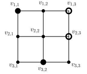
Figure 2: Efficient domination in $P_{3}\Box P_{3}$

In Theorem 2.4 we show the existence of a $2$-packing that results in exactly $\lfloor\frac{n}{3}\rfloor$ voids in $P_{n}\Box P_{3}$. Thereby, it is proved that $F(P_{n}\Box P_{3})=3n-\lfloor\frac{n}{3}\rfloor$ and hence, it is not efficiently dominatable. Further, in Theorem 2.4, for ease of reference we follow a different labeling for the vertices of $P_{n}\Box P_{3}$, than the one mentioned earlier in this section. Upon partitioning the vertices into blocks, label the vertices of each block in $P_{n}\Box P_{3}$ as shown in figure 3. Note that vertices at same positions in different blocks receive similar labels, but are distinguished in terms of the block they belong to. Similar pattern is extended for blocks of larger size.

Figure 3: Labeling of vertices of block $B_{i}$ in $P_{n}\Box P_{3}$

Theorem 2.4.

$P_{n}\Box P_{3}$ is not efficiently dominatable and $F(P_{n}\Box P_{3})=3n-\lfloor\frac{n}{3}\rfloor$.

Proof.

An $F(P_{n}\Box P_{3})$-set is obtained by choosing vertices blockwise as follows: As explained earlier, at most two vertices can be chosen from any $3\times 3$ block. Let $S=\{v_{1,1}^{(i)},v_{3,2}^{(i)}:1\leq i\leq k-2\}$. It can be observed from figure 4 that by the above choice of two vertices from each $B_{i}\,\,(1\leq i\leq k-3)$, the vertex $v_{1,3}^{(i)}$ that appeared as void in $B_{i}$ is later dominated by $v_{1,1}^{(i+1)}$. This results in exactly one void, namely $v_{2,3}^{(i)}$ in each $B_{i}\,\,(1\leq i\leq k-3)$. Next, based on the value of $n$, suitable vertices are chosen from $B_{k-1}$ and $B_{k}$ as explained below:
Case (i): $n\equiv 0\,\,(mod\,\,3)$
Let $S^{\prime}=\{v_{2,1}^{(k-1)},v_{1,3}^{(k-1)}\}\cup\{v_{3,1}^{(k)},v_{2,3}^{(k)}\}$. By this choice, the voids $v_{2,3}^{(k-2)}$, $v_{3,3}^{(k-1)}$ and $v_{1,1}^{(k)}$ that were in $B_{k-2}$, $B_{k-1}$ and $B_{k}$ are later dominated by $v_{2,1}^{(k-1)}$, $v_{3,1}^{(k)}$ and $v_{1,3}^{(k-1)}$ respectively (refer to figure 4). So, $S^{\prime}$ results in exactly one void each in $B_{k-2}$, $B_{k-1}$ and $B_{k}$. Totally there are $\lfloor\frac{n}{3}\rfloor$ blocks and $S\cup S^{\prime}$ results in one void in each block. Hence, $S\cup S^{\prime}$ is a $2$-packing with influence $3n-\lfloor\frac{n}{3}\rfloor$ in $P_{n}\Box P_{3}$.

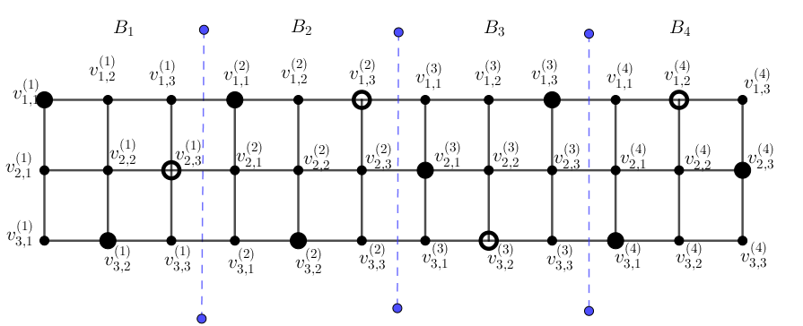
Figure 4: $P_{12}\Box P_{3}$

Case (ii): $n\equiv 1\,\,(mod\,\,3)$
In this case, the last block $B_{k}$ is of size $4\times 4$ (refer to figure 5). Let $S^{\prime\prime}=\{v_{1,1}^{(k-1)},v_{3,2}^{(k-1)}\}\cup\{v_{1,1}^{(k)},v_{3,2}^{(k)},v_{2,4}^{(k)}\}$. Then, by a similar argument as in case (i), $S\cup S^{\prime\prime}$ is a $2$-packing with influence $3n-\lfloor\frac{n}{3}\rfloor$ in $P_{n}\Box P_{3}$, when $n\equiv 1\,\,(mod\,\,3)$ (refer to figure 5).

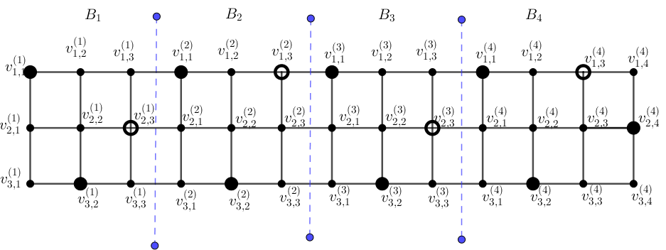
Figure 5: $P_{13}\Box P_{3}$

Case (iii): $n\equiv 2\,\,(mod\,\,3)$
In this case, $B_{k}$ is of size $3\times 5$. With $S^{\prime\prime\prime}=\{v_{1,1}^{(k-1)},v_{3,2}^{(k-1)}\}\cup\{v_{1,1}^{(k)},v_{3,2}^{(k)},v_{1,4}^{(k)},v_{3,5}^{(k)}\}$, it can be shown by a similar argument as in case (i) that $S\cup S^{\prime\prime\prime}$ is a $2$-packing with influence $3n-\lfloor\frac{n}{3}\rfloor$ in $P_{n}\Box P_{3}$, when $n\equiv 2\,\,(mod\,\,3)$ (refer to figure 6).

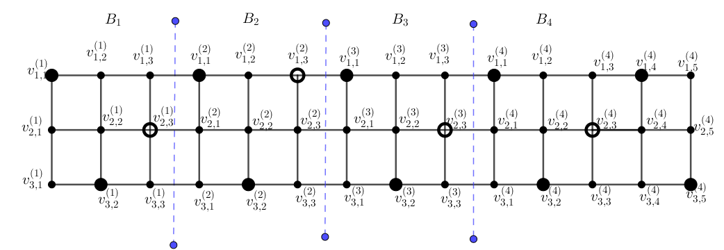
Figure 6: $P_{14}\Box P_{3}$

Thus, in each case, $P_{n}\Box P_{3}$ has a $2$-packing with influence $3n-\lfloor\frac{n}{3}\rfloor$ and it follows from Observation 2.3 that it is the maximum influence of $P_{n}\Box P_{3}$. Hence, the result follows. ∎

The next proposition deals with efficient domination in square grids of sizes $4$, $5$, and $6$ and the results follow trivially (refer to figures 7(a), 7(b) and 7(c)).

Proposition 2.5.

• $P_{4}\Box P_{4}$ is efficiently dominatable.

• $P_{5}\Box P_{5}$ is not efficiently dominatable and $F(P_{5}\Box P_{5})=23.$

• $P_{6}\Box P_{6}$ is not efficiently dominatable and $F(P_{6}\Box P_{6})=33.$

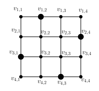
(a) $P_{4}\Box P_{4}$

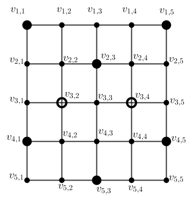
(b) $P_{5}\Box P_{5}$

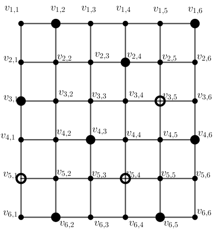
(c) $P_{6}\Box P_{6}$

Figure 7: Efficient domination in square grids of sizes 4, 5, and 6

Next in Theorem 2.7, we discuss the notion of efficient domination in $P_{n}\Box P_{m}$, for $n,m\geq 7$. Later using the proof technique adopted in this theorem and Proposition 2.5, we characterize the efficiently dominatable rectangular grids $P_{n}\Box P_{m}$, for $n,m\geq 3$. The following observation supports the discussions in Theorem 2.7.

Observation 2.6.

Suppose that $P_{n}\Box P_{m}$ ($n,m\geq 7$) is partitioned into blocks of suitable sizes and we identify vertices from each block to include in an $F(P_{n}\Box P_{m})$-set. Then, choosing vertices from a $3\times 3$ block as in either figure 8(a) (choosing $v_{i,j}$ and $v_{i+2,j+2}$) or figure 8(b) (choosing $v_{i,j}$ and $v_{i+2,j+2}$) will create a void in that block, at a vertex of degree four. In such cases, these voids cannot be further dominated by any other adjacent block in $P_{n}\Box P_{m}$, unlike the cases discussed earlier in Theorem 2.4. Hence, if such voids occur independently in any (sub)block of size $3\times 3$, they will continue to be voids in $P_{n}\Box P_{m}$.

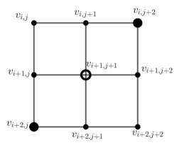
(a)

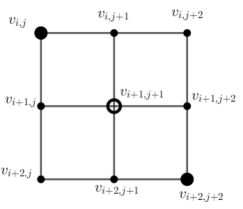
(b)

Figure 8: $2$-packings of $P_{3}\Box P_{3}$ creating a void at a vertex of degree four

Theorem 2.7.

If $n\geq 7$ and $m\geq 7$, then $P_{n}\Box P_{m}$ is not efficiently dominatable.

Proof.

Let $S$ be an $F(P_{n}\Box P_{m})$-set. If possible, assume that $I(S)=nm$. Then, $|N[v_{i,j}]\cap S|=1$, for each $v_{i,j}\in V(P_{n}\Box P_{m})$. Choose an arbitrary vertex, say $v_{1,1}$. Then, either $v_{1,1}\in S$ or exactly one of its neighbors, namely, $v_{1,2}$ or $v_{2,1}$ must be in $S$. The above three cases are discussed in detail as below:
Case (i): $v_{1,1}\in S$
If $v_{1,1}\in S$, then to dominate $v_{2,2}$, either $v_{2,3}$ or $v_{3,2}$ must be in $S$. Suppose $v_{2,3}\in S$, then to dominate $v_{3,1}$, $v_{4,1}\in S$. But, choosing $v_{2,3}$ and $v_{4,1}$ to include in $S$ results in a $3\times 3$ block in which the vertices are dominated as in figure 8 (a) (with $i=2,\,\,j=1$). Then, it follows from Observation 2.6 that $N[v_{3,2}]\cap S=\emptyset$, which is a contradiction.
On the other hand, if $v_{3,2}\in S$, then by a similar argument as above, to dominate $v_{1,3}$, $v_{1,4}\in S$. This choice of vertices results in a $3\times 3$ block with domination as in figure 8 (a) (with $i=1,\,\,j=2$). Hence, $N[v_{2,3}]\cap S=\emptyset$, which is a contradiction.

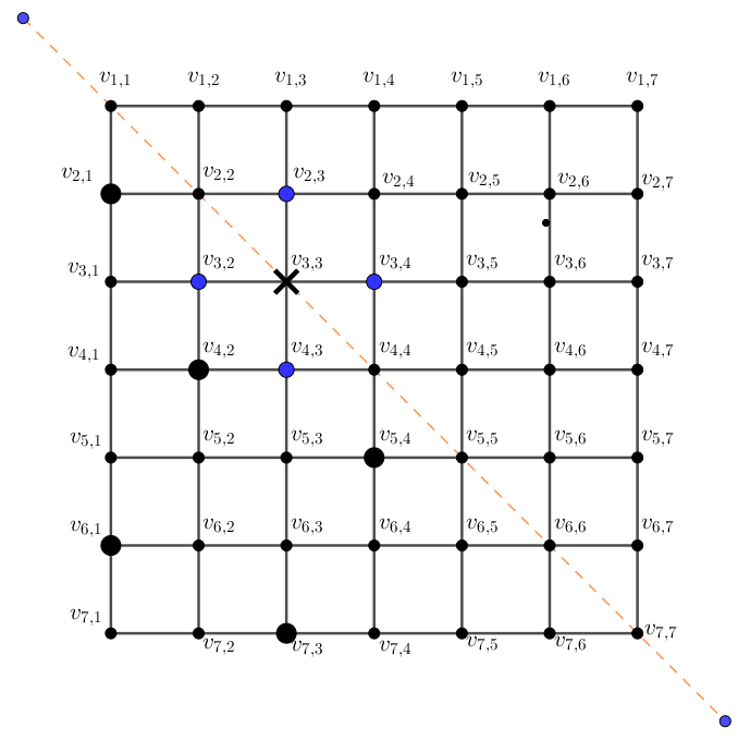
Figure 9: Efficient domination in $P_{7}\Box P_{7}$

Case (ii): $v_{2,1}\in S$
To dominate $v_{4,1}$, either $v_{5,1}$ or $v_{4,2}\in S$. If $v_{5,1}\in S$, then to dominate $v_{3,2}$, $v_{3,3}$ must be in $S$. This results in a $3\times 3$ block with domination as in figure 8 (a) (with $i=3,\,\,j=1$). Consequently, $N[v_{4,2}]\cap S=\emptyset$, leading to a contradiction. So, let $v_{4,2}\in S$. Then, to dominate $v_{5,1}$, $v_{6,1}\in S$. Next, to dominate $v_{6,3}$, either $v_{6,4}$ or $v_{7,3}\in S$.
If $v_{6,4}\in S$, then it results in a $3\times 3$ block with domination as in figure 8 (b) (with $i=4,\,\,j=2$). Hence, $N[v_{5,3}]\cap S=\emptyset$, leading to a contradiction.
So, let $v_{7,3}\in S$. Then, to dominate $v_{5,3}$ we are left with only one choice, namely, $v_{5,4}$ to include in $S$. At this stage, $S=\{v_{2,1},v_{4,2},v_{6,1},v_{7,3},v_{5,4}\}$. But, to dominate $v_{3,3}$, we are left with no choice as all its neighbors are at distance $1$ or $2$ from $S$ (refer to figure 9). Hence, $N[v_{3,3}]\cap S=\emptyset$, which is again a contradiction.
Case (iii): $v_{1,2}\in S$
Since there is an automorphism $f(v_{i,j})=v_{j,i}$ of $P_{n}\Box P_{m}$ that maps $v_{2,1}$ to $v_{1,2}$, the argument made in case(ii) can be modified accordingly. This results in $S=\{v_{1,2},v_{2,4},v_{1,6},v_{3,7},v_{4,5}\}$ in $S$. But, as discussed in case (ii), to dominate $v_{3,3}$, we are left with no choice as all its neighbors are at distance $1$ or $2$ from $S$. Hence, $N[v_{3,3}]\cap S=\emptyset$, which is a contradiction.
Summarizing the above arguments, it can be observed that each of these cases resulted in a void in $P_{n}\Box P_{m}$, whcih cannot be further dominated by any adjacent block. In particular, such a void is created in a $7\times 7$ block of $P_{n}\Box P_{m}$ (i.e., considering the first seven rows and the first seven columns). As $P_{7}\Box P_{7}$ is an induced subgraph of $P_{n}\Box P_{m}$, for all $n\geq 7$ and $m\geq 7$, $P_{n}\Box P_{m}$ is not efficiently dominatable when $n,m\geq 7$. ∎

The efficient domination in the grids $P_{n}\Box P_{4}$ for $n>4$, $P_{n}\Box P_{5}$ for $n>5$ and $P_{n}\Box P_{6}$ for $n>6$ can be studied by similar arguments as in Theorem 2.7 and we arrive at the following result.

Theorem 2.8.

For $4\leq m\leq 6$ and $n>m$, $P_{n}\Box P_{m}$ is not efficiently dominatable.

The results discussed above in Theorem 2.2 to Theorem 2.8 lead to the following characterization for efficiently dominatable grid graphs.

Corollary 2.9.

If $n\geq 3$ and $m\geq 3$, then $P_{n}\Box P_{m}$ is efficiently dominatable if and only if $n=m=4$.

Next, using Construction 2.10 discussed below, we derive a lower bound on $F(P_{n}\Box P_{n})$ for $n\geq 7$. The bound is obtained by constructing a $2$-packing which dominates all vertices of $P_{n}\Box P_{n}$, except a few vertices at the boundaries. Interestingly, it is evident from Table 1 that the $2$-packing obtained in the construction is nearly optimal (that is, most likely an $F(P_{n}\Box P_{n})$-set), as equality in the derived lower bound is attained for most values of $n$. In addition, the construction helps in generalizing the efficient domination property in the infinite cases disucssed in Section 2.3. An illustration of the construction is shown in figure 10 for $P_{9}\Box P_{9}$ and it is easy to extend the construction for any $n\geq 7$.

Figure 10: Efficient domination in $P_{9}\Box P_{9}$

Construction 2.10.

For $n\geq 7$, we obtain a nearly optimal $2$-packing for $P_{n}\Box P_{n}$ as follows:

• Initially, select vertices from the first and second columns alternatively and at each selection, pick up a pair of vertices, namely, $(v_{i,1},v_{i+2,2})$. Depending on the value of $n$, we start from either first or second row. Precisely, if $n=5k+4\,\,(k\in\mathbb{N})$, start with $v_{2,1}$. Else, start with $v_{1,1}$.

• Upon choosing each pair, skip two rows inbetween and proceed with the selection of next pair. For example, if $n=5k+4,$ the first pair is with $(v_{2,1},v_{4,2})$ and leaving two rows inbetwen, the second pair is $(v_{7,1},v_{9,2})$, third pair is $(v_{12,1},v_{14,2})$ and so on (refer to figure 10). Continue this selection until all rows are covered. Note that the last choice may be either a pair of vertices or a single vertex in first column.

• Let $x$ be the last vertex (may be from first column or second column) chosen in the above process. Based on the choice of $x$, we select a vertex $y$ from the last row as below:
  Case(i) : Suppose $x$ is $v_{n-2,2}$, then $y=v_{n,3}$. Case(ii) : Suppose $x$ is $v_{n-1,2}$, then $y=v_{n,5}$. Case(iii) : Suppose $x$ is $v_{n-1,1}$, then $y=v_{n,4}$. Case(iv) : Suppose $x$ is $v_{n,1}$, then $y=x=v_{n,1}$. Case(v) : Suppose $x$ is $v_{n,2}$, then $y=x=v_{n,2}$. (Occurs when $n=5k+4$)

• Upon fixing $y$ as above, select the vertices on the last row which are at a distance of $\{5k|k=1,2,\dots,\lfloor\frac{n}{5}\rfloor\}$ from $y$.

• Next, for each $v_{i,j}$ selected in above steps, choose the vertices $\{v_{i-k,j+2k}:k\in\mathbb{N}\}$ until the boundary is reached. The choice is analogous to a knight placed at $v_{i,j}$ moving towards east (two-step right, one step up) repeatedly.

It is evident from the above choice of vertices that the set of vertices generated at the end forms a $2$-packing of $P_{n}\Box P_{n}$, where $n\geq 7$ (refer to figure 10).

Number of voids generated by the above $2$-packing:

To compute the number of voids generated by the above $2$-packing, the following observations are noted:

• The vertices are included in $S$ in such a way that all vertices of $P_{n}\Box P_{n}$ are dominated exaclty once by $S$, except a few that lie on the boundaries. Hence, voids occur only at the boundaries, that is, on the rows $R_{1}$, $R_{n}$ and the columns $C_{1}$, $C_{n}$.

• It follows from the construction that such voids occur either between a pair of vertices in $S$ which are at distance five apart or at corners or at distance two from corner vertices.

• For instance, if $v_{1,j},v_{1,q}\in S\cap R_{1}$, then $d(v_{1,j},v_{1,q})=5$. Since $v_{1,j}$ and $v_{1,q}$ dominate their respective neighbors in $R_{1}$, out of the four internal vertices lying on the path between $v_{1,j}$ and $v_{1,q}$, possibly, there are at most two voids between $v_{1,j}$ and $v_{1,q}$. But, in cases where one of their neighbors in the adjacent row, namely, $R_{2}$ is in $S$, then the number of voids reduces to one. Similar arguments hold for $R_{n}$, $C_{1}$ and $C_{n}$. The number of such pairs of vertices at distance five on the boundaries and consequently, the number of voids depends on the value of $n$, as discussed in detail below:

• Case (i): $n\equiv 0\,\,(mod\,\,5)$ or $n=5k$
  In this case, $k$ vertices from each of $C_{1}$ and $R_{n}$ belong to $S$, resulting in a total of $2k$ voids on $C_{1}$ and $R_{n}$. Similarly, $k$ vertices from each of $C_{n}$ and $R_{1}$ belong to $S$, resulting in a total of $2k$ voids. Hence, if $n=5k$, then $S$ generates $4k$ voids in $P_{n}\Box P_{n}$, for $n\geq 7$.

• Case (ii): $n\equiv 1\,\,(mod\,\,5)$ or $n=5k+1$
  In this case, $k+1$ vertices from each of $R_{1}$,$C_{1}$,$R_{n}$ and $C_{n}$ belong to $S$, resulting in $k$ voids on each. Hence, totally $4k$ voids are generated by $S$, if $n=5k+1$.

• Case (iii): $n\equiv 2\,\,(mod\,\,5)$ or $n=5k+2$
  In this case, $k+1$ vertices from each of $R_{1}$ and $C_{1}$ belong to $S$, generating $k$ voids on each. And, $k$ vertices from $R_{n}$ and $C_{n}$ belong to $S$, leading to a total of $2k+1$ voids. Hence, totally $4k+1=n-k-1$ voids are generated by $S$, when $n=5k+1$.

• Case (iv): $n\equiv 3\,\,(mod\,\,5)$ or $n=5k+3$
  Here, $k+1$ vertices from each of $R_{1}$, $R_{n}$ and $C_{1}$ belong to $S$, resulting in a total of $3k+1$ of voids. Further, $k$ vertices from $C_{n}$ are in $S$, leading to $k+1$ voids. Hence, a total of $4k+2=n-k-1$ voids are generated by $S$.

• Case (v): $n\equiv 4\,\,(mod\,\,5)$ or $n=5k+4$
  In this case, $k+1$ vertices from each of $R_{1}$,$C_{1}$,$R_{n}$ and $C_{n}$ belong to $S$. This results in $k$ voids on each and hence, a total of $4k$ voids are generated by $S$.
  

For $n=9$, the pattern of selection is shown in figure 10 and it can be observed that the voids occur at the edges or boundaries. Following the above discussion, Table 1 gives the number of voids $(n^{2}-I(S))$ for $7\leq n\leq 22$, where $S$ is the $2$-packing obtained using Construction 2.10. In fact, for each $7\leq n\leq 22$, it is observed that the influence of $S$ obtained above is maximum and is equal to $F(P_{n}\Box P_{n})$.

Table 1: Number of voids in $P_{n}\Box P_{n}$

Construction 2.10 guarantees the existence of a $2$-packing for $P_{n}\Box P_{n}$ $(n\geq 7)$ resulting in the number of voids as discussed above. This leads to the following lower bound for $P_{n}\Box P_{n}$, when $n\geq 7$.

Theorem 2.11.

For $n\geq 7$ and $k=\lfloor\frac{n}{5}\rfloor$,

$F(P_{n}\Box P_{n})\geq\begin{cases}n^{2}-4k;&\mbox{if $n\equiv$ 0 or 1 or 4 (mod 5)}\\ {n^{2}-n+k+1};&\mbox{if $n\equiv$ 2 or 3 (mod 5)}\end{cases}$

As mentioned earlier, it is observed that the bound given in Thorem 2.11 is attained for most values of $n\geq 7$. Based on this, we state the following conjecture.

Conjecture 2.12.

For $n\geq 7$ and $k=\lfloor\frac{n}{5}\rfloor$,

$F(P_{n}\Box P_{n})=\begin{cases}n^{2}-4k;&\mbox{if $n\equiv$ 0 or 1 or 4 (mod 5)}\\ {n^{2}-n+k+1};&\mbox{if $n\equiv$ 2 or 3 (mod 5)}\end{cases}$

2.3 Infinite lattice graphs

The construction of a $2$-packing discussed for a finite rectangular grid in the previous section resulted in voids at the boundaries. The vertices included in the $2$-packing lie on the diagonal lines as shown in figure 10. This pattern can also be extended for an infinite rectangular grid and for an infinite triangular grid. The infinite hexagonal grid has another interesting pattern which is discussed in Section 2.3.3.

2.3.1 Infinite Rectangular grid

As mentioned earlier, a rectangular grid that is bounded on the three sides (top, left and right) and unbounded at the bottom is referred to as $P_{n}\Box P_{\infty}$, where $1\leq n<\infty$. The one which is bounded on the two sides (top and left) and unbounded at right and bottom is referred to as $P_{\infty}\Box P_{\infty}$.

It is noted that Table 1 depicts a pattern in the difference between the number of voids for consecutive values of $n$ as follows: $(+1,-2,+4,0,+1)$, $(+1,-2,4,0,+1)$ $\dots$ Hence, as $n$ increases or as $n\rightarrow\infty$, the number of voids keep oscillating and does not coverge to zero. Consequently, the grids $P_{n}\Box P_{\infty}$ for $1\leq n\leq\infty$ and $P_{\infty}\Box P_{\infty}$ are not efficiently dominatable.

In the next result, extending construction 2.10, we prove that an infinite rectangular grid (unbounded on all four sides) is efficiently dominatable.

Theorem 2.13.

An infinite rectangular grid is efficiently dominatable.

Proof.

Let $G$ denote an infinite rectangular grid. Construct an EDS $S$ for $G$ as follows: Start with an arbitrary vertex, say, $v_{i,j}$ and let $S=\{v_{i,j}\}$. Next, add the four vertices $v_{i+1,j-2},v_{i+2,j+1},v_{i-1,j+2}$, $v_{i-2,j-1}$ to $S$, if they are already not in $S$. Since $d(v_{i,j},v_{p,q})=|i-p|+|j-q|$, it can be observed that all these four vertices are at distance three from $v_{i,j}$ and they are also mutually at distance at least three. Hence, $S=S\cup\{v_{i+1,j-2},v_{i+2,j+1},v_{i-1,j+2},v_{i-2,j-1}\}$ is a $2$-packing of $G$. Next, for each vertex $v_{p,q}$ in $S$, select another set of four vertices in the same manner as above and add them to $S$. The vertices are chosen in such a way that distance between any two vertices in $S$ is at least three and hence, the set $S$ so obtained forms a $2$-packing of $G$. Note that the vertices in $S$ lie on the diagonal lines as shown in figure 11. Pairing the vertices of $S$ lying on consecutive diagonal lines to form opposite corners of $2\times 3$ grids as in figure 12, it can be observed these $2\times 3$ grids are disjoint and there are no voids between the diagonal lines. Since $G$ is infinite (or unbounded on all sides), this pattern of adding vertices to $S$ shall continue iteratively so that all vertices of $G$ are dominated, resulting in no void. Hence, the set $S$ so obtained is an EDS of $G$ or equivalently, $G$ is efficiently dominatable. ∎

Figure 11: Efficient domination in an Infinite rectangular grid

Figure 12: Disjoint $2\times 3$ grids

Construction 2.14.

Existence of efficiently dominatable near-Grid graphs:
Note that in figure 11, the intersections of two lines correspond to vertices. The subtructure $P_{11}\Box P_{11}$ of an infinite grid is highlighted using bold lines. Independently examining the grid $P_{11}\Box P_{11}$, it can be observed that there exists an $F(P_{11}\Box P_{11})$-set resulting in voids which lie on the boundaries as shown in figure 11. These voids can be dominated by adding new vertices, one to dominate each void so that the resultant graph is efficiently dominatable. In general, given a grid $P_{n}\Box P_{n}$, where $n\geq 7$, if there $k$ voids generated by an $F(P_{n}\Box P_{n})$-set, then by arranging them suitably to lie on the boundaries, we can add $k$ new vertices and make them adjacent to one void each. Then, the resultant graph becomes efficiently dominatable. This results in a new class of efficiently dominatable graphs which are nearly grid graphs.

2.3.2 Infinite Triangular grid

A triangular grid graph is formed by triangular tessellations. We label the $j^{th}$ vertex in the $i^{th}$ row of a triangular grid as $v_{i,j}$ (refer to figure 13). By following the same procedure explained for an infinte rectangular grid in Section 2.3.1, we can construct an EDS for an infinite triangular grid. For ease of reference, we refer to an infinite triangular grid by $T_{\infty}$.

Figure 13: Labeling of a Triangular Grid

Theorem 2.15.

An infinite triangular Grid is efficiently dominatable.

Proof.

We construct an EDS, say $S$, of $T_{\infty}$ as follows: Choose an arbitrary vertex, say $v_{i,j}$, and let $v_{i,j}\in S$. Select the four vertices $v_{i-1,j+2}$, $v_{i+1,j-2}$, $v_{i+2,j}$ and $v_{i-2,j}$ around $v_{i,j}$ as shown in figure 14. Clearly, these four vertices are at distance three from $v_{i,j}$ and are at mutually at distance at least three (refer to figure 14). Hence, the set $S=S\cup\{v_{i-1,j+2},v_{i+1,j-2},v_{i+2,j},v_{i-2,j}\}$ will be a $2$-packing of $T_{\infty}$. Next, for each vertiex $v_{p,q}\in S$, choose another set of four vertices in the same manner and add them to $S$. The chosen vertices are in such a way that they are mutually at distance at least three and they all fall on the diagonal lines as shown in the figure 15. Hence, the set $S$ so generated forms a $2$-packing of $T_{\infty}$. Further, pairing the vertices of consecutive diagonal lines to form opposite corners of disjoint $3\times 2$ triangular grids (that is, grids containing 3 rows with each row containing 2 vertices), it can be observed that these vertices dominate every vertex between the diagonal lines and no voids are created. As the grid is infinite, it is possible to iteratively continue this pattern of choosing vertices along all directions and add to $S$. Based on the way the vertices are selected, it can be observed the set $S$ obtained at each iteration is a $2$-packing of $T_{\infty}$ and all vertices between the diagonal lines are dominated (refer to figure 15). Hence, the final set $S$ so obtained will be an EDS of $T_{\infty}$. ∎

Figure 14: Choice of vertices in an infinite triangular grid

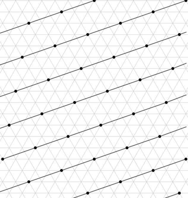
Figure 15: EDS of an Infinite triangular grid

2.3.3 Infinite hexagonal grid

A hexagonal grid graph is formed by tessellations of hexagons. We know that $C_{6}$ is an efficiently dominatable graph and any two diagonally opposite vertices form an EDS of $C_{6}$. This property forms the basis for constructing an EDS for an infinite hexagonal grid. For conveninece, we use $H_{\infty}$ to refer to an infinite hexagonal grid.

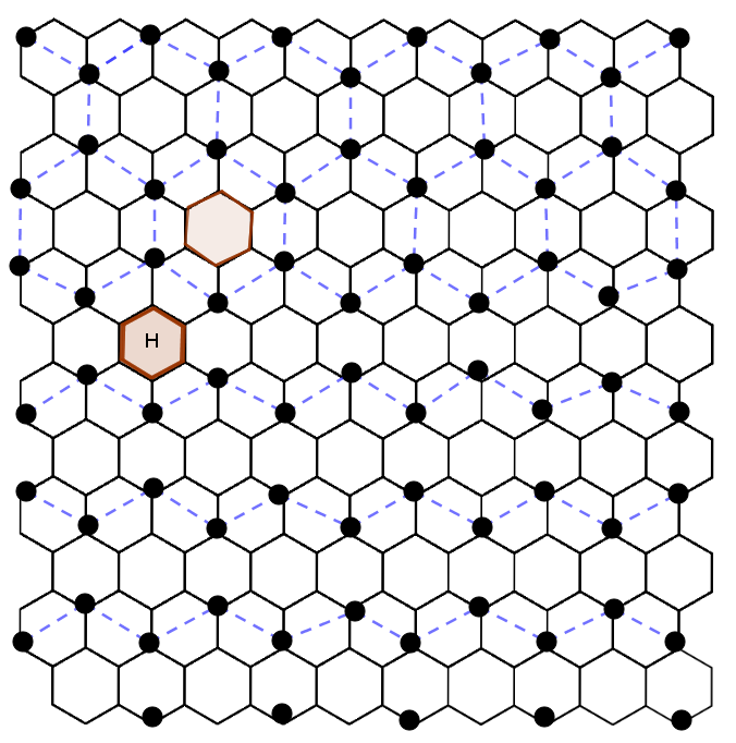
Figure 16: EDS of an infinite hexagonal grid

Theorem 2.16.

An infinite hexagonal grid is efficiently dominatable.

Proof.

We construct an EDS, say $S$, of $H_{\infty}$ as follows: Note that each vertex in an infinite hexagonal grid lies in (or common to) three adjacent hexagons. Choose an arbitrary vertex, say $v$, and let $v\in S$. Next, from each of the three hexagons to which $v$ belongs, select the vertices which are at distance $3$ from $v$ (that is, the vertex diagonally opposite to $v$ in each hexagon containing $v$). Add these three vertices to $S$. Note that the set $S$ generated at this stage is a $2$-packing as all its vertices are mutually at distance at least three in $H_{\infty}$ (refer to figure 16). Next, for each of the newly added vertices, repeat the process of choosing the diagonally opposite vertices from the hexagons they belong to. This process of constructing a $2$-packing for $H_{\infty}$ results in a structure as shown in figure 16. It can be observed that all those vertices in $S$ are mutually at distance at least three and they lie on the zig-zag lines. It can be noted that for any hexagon, either two diagonally opposite vertices lie on these lines or no vertex lies on these lines. Suppose no vertex of a hexagon $H$ belongs to $S$, then each vertex of $H$ is dominated by a unique neighbor outside $H$. Thereby, the set $S$ so generated dominates all vertices of $H_{\infty}$ and hence, $S$ is a EDS of $H_{\infty}$. ∎

3 Conclusion

In this paper, the concept of efficient domination has been studied on lattice graphs, namely rectangular grid graphs, triangular grid graphs, and hexagonal grid graphs. A characterization is obtained for efficiently dominatable finite rectangular grids. A finite square grid $P_{n}\Box P_{n}$ has been shown to efficiently dominatable if and only if $n=4$. For those finite square grids which are not efficiently dominatable, a lower bound on its efficient domination number is derived. A contructive procedure is given to derived these lower bounds and the construction could be extended to both infinite rectangular grids and infinite triangular grids to prove that they are efficiently dominatable. The lower bound derived is found to be attained at most values of $n$, based on which a conjecture is stated. Another constructive procedure has been discussed to study the notion of efficient domination in infinite hexagonal grids. The study on finite triangular and hexagonal grid structures is in progress.

References

- [1] Bange, D., Barkauskas, A., and Slater, P (1978) Disjoint dominating sets in trees, Technical Report 78-1087J, Sandia Laboratories.
- [2] Bange, D., Barkauskas, A., and Slater, P (1988) Efficient dominating sets in graphs, Appl. Disc. Math., 189-199.
- [3] Goddard, W., Oellermann, O., Slater, P., Swart, H. (2000). Bounds on the total redundance and efficiency of a graph. Ars Combinatoria, 54, 129-138.
- [4] Lu, C. L., Tang, C. Y. (2002). Weighted efficient domination problem on some perfect graphs. Discrete Applied Mathematics, 117 (1-3), 163-182.
- [5] Abay-Asmerom, Ghidewon, Richard H. Hammack, and Dewey T. Taylor (2009) Perfect r-codes in strong products of graphs. Bull. Inst. Combin. Appl, 55, 66-72.
- [6] Chang, Tony Yu, and W. Edwin Clark (1993) The domination numbers of the and grid graphs. Journal of Graph Theory, 17 (1), 81-107.
- [7] Gravier, Sylvain, and Michel Mollard (1997) On domination numbers of Cartesian product of paths. Discrete applied mathematics, 80 (2-3), 247-250.
- [8] Gonçalves, Daniel, Alexandre Pinlou, Michaël Rao, and Stéphan Thomassé (2011) The domination number of grids. SIAM Journal on Discrete Mathematics, 25 (3), 1443-1453.
- [9] Milanič, M. (2013). Hereditary efficiently dominatable graphs. Journal of Graph Theory, 73 (4), 400-424.
- [10] Barbosa, R. and Slater, P (2016) On the efficiency index of a graph. Journal of Combinatorial Optimization, 31 (3), 1134-1141.
- [11] Biggs, N (1973) Perfect codes in graphs, Journal of Combinatorial Theory, Series B, 15 (3), 289-296.
- [12] Chelvam, T. T. and Mutharasu, S (2011) Efficient domination in cartesian products of cycles. Journal of Advanced Research in Pure Mathematics, 3 (3), 42-49.
- [13] Acharya, B. D., and M. K. Gill (1981) On the index of gracefulness of a graph and the gracefulness of two-dimensional square lattice graphs. Indian J. Math, 23 (14), 81-94.
- [14] Vaishampayan, Vinay A., Neil JA Sloane, and Sergio D. Servetto (2001) Multiple-description vector quantization with lattice codebooks: Design and analysis. IEEE Transactions on Information Theory 47 (5), 1718-1734.
- [15] Haynes, T. W., Hedetniemi, S., and Slater, P (1998) Fundamentals of domination in graphs, New York: Marcel Dekker, Inc.
- [16] Imrich, W. and Klavžar, S (2000) Product graphs: Structure and Recognition, Wiley.
- [17] Livingston, M. and Stout, Q. F (1988) Distributing resources in hypercube computers, In The third conference on Hypercube concurrent computers and applications: Architecture, software, computer systems, and general issues, ACM-1, 222-231.
- [18] Livingston, M. and Stout, Q. F (1990) Perfect dominating sets. Congr. Numer., 79, 187-203.
- [19] West, D. B (2001) Introduction to graph theory, Pearson Education, India, 2nd edition.
- [20] Yen, C.-C. and Lee, R. C (1996) The weighted perfect domination problem and its variants. Discrete Applied Mathematics, 66 (2), 147-160.