Gluons, light and heavy quarks and their interactions in the instanton vacuum

Abstract

The interactions of colorful particles with QCD vacuum instantons are controlled by the instanton size $\rho$ and inter-instanton distance $R$, which are the main parameters of Instanton Liquid Model (ILM) of the QCD vacuum. Lattice, theoretical and phenomenological estimates show that the values of these parameters are $\rho\approx 1/3$ fm and $R\approx 1$ fm, and the corresponding packing parameter $\kappa=\rho^{4}/R^{4}\approx 0.01$. The strength of the light quark-instanton interaction is sizable and close to that of the gluon-instanton one. They are related to the dynamical light quark mass $M_{q}$ and dynamical gluon mass $M_{g}$, which are given by $M_{q}\approx M_{g}\approx 360$ MeV$\sim\kappa^{1/2}\rho^{-1}$. On the other hand, the strength of the heavy quark-instanton interaction is weak, and is determined by the direct instanton contribution to the heavy quark mass $\Delta M_{Q}^{{\rm dir}}\approx 70$ MeV$\sim\kappa\rho^{-1}.$ So, the instantons are responsible for mutual interactions among colored particles which are crossing the field of the same instanton, like for example t’Hooft-like interactions of $N_{f}$ light quarks ($N_{f}$ is the light quark flavors number). The light quark propagators in the instanton field have zero modes, which give dominant contributions. Within ILM we are able to derive the light quarks determinants and the light quarks partition function. These tools perfectly describe the light quark physics and its most important and basic phenomena - the spontaneous breaking of the chiral symmetry (SBChS). This allows to understand in details the effective low-energy Chiral Perturbation Theory (ChPT) in terms of quark degrees of freedom, and make unambiguous predictions of the Gasser-Leuteyller low-energy coupling constants. We conclude that ILM is a good framework for the light hadrons physics calculations. This framework allows us to find the properties of light and heavy quarks interactions by accounting of the light quarks determinant in ILM heavy quark correlators. ILM provides the framework for the calculation of SBChS traces in light-heavy quarks systems. As an example, we are considering the process of pions emission by excited heavy quarkonium states. We found a sizable corrections ( $\sim 20\%$) to the widely used dipole approximation for the process $\psi(2S)\rightarrow J/\psi\,\pi^{+}\pi^{-}$. So, we need to find heavy $Q\bar{Q}$ quarkonia spectra and their wave functions. Here we have interplay of two scales: short ($\sim(M_{Q}v)^{-1}\leq 0.15$ fm) perturbative QCD and large ($\sim(M_{Q}v^{2})^{-1}\sim 0.5$ fm) nonperturbative QCD scales, where $v$ is the velocity in $Q\bar{Q}$. We calculate the heavy quarks correlators with perturbative corrections within ILM. We find almost complete mutual cancellation of the ILM direct $O(\kappa)$ instanton and ILM perturbative $O(\kappa^{1/2}\alpha_{s})$ contributions to the heavy quark correlators.

I Introduction

The QCD vacuum is quite nontrivial non-perturbative quantum state characterized by the nonvanishing gluon and light quark condensates, which are well described within the Instanton Liquid Model (ILM) (see reviews [1, 2, 3]). The most essential assumption of ILM is the applicability of the semiclassical approximation, which means that the effective strong coupling $\alpha_{s}$ is rather small. The ILM is characterized by only two parameters: the average instanton size $\rho\approx 0.3\,{\rm fm}$ and the average inter-instanton distance $R\approx 1\,{\rm fm}$. These essential parameters were suggested by Shuryak [4] (see also [1, 2]) and were estimated phenomenologically in [5] (see also [3]). These values are in agreement with lattice measurements [12, 13, 14, 15], and lead to a comfortable value of the packing parameter $\kappa=\rho^{4}/R^{4}\sim 0.01$, which characterizes the fraction of the 4D space occupied by instantons. Such small value of $\kappa$ simplifies very much the calculations within ILM.

One of the most prominent achievements of the Instanton Liquid Model is the correct description of the spontaneous breaking of the chiral symmetry (SBChS), which is responsible for properties of light quark hadrons and nuclei (see reviews [1, 2, 3]). The SBChS is due to specific nonperturbative properties of the QCD vacuum, and is a very important object of investigations by methods of Nonperturbative Quantum Chromo Dynamics (NPQCD). In the instanton picture the SBChS occurs due to the delocalization of single-instanton quark zero modes in the instanton medium, which is possible since current light quark mass $m_{q}\ll 1/\rho$. All properties of light quark physics in ILM are controlled by a rather large value of light quark-instanton interaction effective strength, which is proportional to dynamical light quark mass $M_{q}\sim\kappa^{1/2}\rho^{-1}$. At typical values of the ILM parameters given above, this mass is given by $M_{q}\approx 360$ MeV. In contrast to this, the heavy quark physics is controlled mainly by the heavy quark mass $M_{Q}\gg\rho^{-1}$, with rather small influence of the instantons, since heavy quark-instanton interaction strength is given by $\Delta M_{Q}^{{\rm dir}}\approx 70$ MeV$\sim\kappa\rho^{-1}$.

In this context, we expect that essential properties of open heavy flavor hadrons seem to be strongly governed by such light quark properties as the phenomenon of spontaneous breaking of the chiral symmetry, which should be taken into account in an appropriate way. Consequently, the traces of the nonperturbative dynamics may be essential in the open heavy flavor systems not only for their decay modes into the lighter hadrons, but also for studies of their static properties. Similar effects are expected in the decay processes of exited heavy quarkonia, with emission of light hadrons.

In contrast, the heavy quarkonia spectrum and their wave functions could be affected by both perturbative and non-perturbative interaction forces [70, 71]. In ILM we have to take into account the $Q\bar{Q}$ perturbative potential with the modification of gluon properties due to presence of instantons in QCD vacuum together with direct instanton generated one  [77]. We have to note that, instanton media induced dynamical gluon mass $M_{g}\approx 360$ MeV$\sim\kappa^{1/2}\rho^{-1}$, which tells us that perturbative gluon-instanton interaction strength is the same as for light quarks and is large.

The overview of current situation is also one of the aims of the present review and will be done on a basis several recent studies [74, 75, 76, 77] developed in the framework of instanton liduid model (ILM) of QCD vacuum. We organize our review as follows: in the subsection I.1 of the Introduction we briefly remind the main concepts of the instanton liquid model (ILM) for QCD vacuum and its phenomenological parameters. The section II is devoted to discussion of the physics of the light quarks in ILM. In the subsection II.1 of that section we focus on the derivation of chiral light mesons effective action in the presence of external fields for the case of light quarks number $N_{f}=2$. The most essential part of our review is the section III, in which we consider the heavy and light quarks systems in ILM. In its subsection III.1 we calculate the strength of heavy-quark-instanton interaction, and in the following subsection III.2 we consider the instanton-generated heavy and light quark interactions in ILM. The subsection III.3 is devoted to the heavy quarkonium and light quarks interactions in ILM, where it is derived the effective action corresponding to the processes of pions emission by heavy quarkonium. In the subsection III.4 we compare the heavy quarkonium states and instanton sizes to clarify in the following subsection III.5 the mechanism of the $(Q\bar{Q})_{n^{\prime}}\rightarrow(Q\bar{Q})_{n}\,\,\pi\pi$ processes. From our estimates we have a sizable correction $\sim 20\%$ to the standard dipole approximation for the case of $\psi^{\prime}\rightarrow J/\psi\pi\pi$ process. In order to make precise calculations of this and similar processes, we have to calculate the quarkonium spectrum and wave functions within ILM. It requires the calculations of heavy quark correlators with perturbative $O(\alpha_{s})$ corrections in ILM, which are considered in the section IV. In the subsection IV.1 the gluon propagator is calculated within ILM, which is used in the subsection  IV.2 for the calculations of ILM perturbative corrections to the heavy quark mass and in the subsection IV.3 is applied to the calculations of heavy quarks $Q\bar{Q}$ singlet potential with perturbative corrections in ILM.

In the section V we give an overview of the ILM results and formulate the direction of the following research.

I.1 Instanton liquid model (ILM) for QCD vacuum and its parameters

The instanton is one of the possible manifestations of the rich topological structures of QCD vacuum. Mathematically, an instanton is a topologically non-trivial classical solution of the Yang-Mills equations in the 4-dimensional Euclidean space, and mathematically corresponds to the mapping of $SU(2)$ part of internal $SU(N_{c})$ color space to the appropriate $SU(2)$ part of the 4-dimensional Euclidean space.

The potential part of the classical Yang-Mills action has periodic dependence on the collective coordinate, which is called the Chern-Simons (CS) number $N_{{\rm CS}}$. The classical vacuum, being defined as minimum energy state, is infinitely degenerated set of solutions which differ by this choice of $N_{{\rm CS}}=n\in\mathbb{Z}$, as could be seen from the Fig. 1. It can be also considered as the lowest energy quantum state of the one-dimensional periodic crystal along the CS coordinate [6, 7]. In this context, the instanton might be considered as a tunneling path, which joins adjacent classical vacua with Chern-Simons indices $n$ and $n+1$, while the anti-instanton corresponds to transition in opposite direction [8].

,

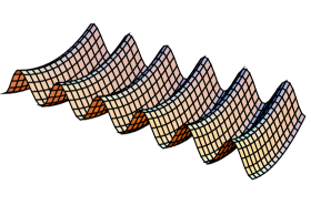
Figure 1: Left plot: Schematic illustration of the periodic dependence of potential energy on Chern-Simons number $N_{{\rm CS}}$, and mild (oscillator-like) growth in all other directions in functional space [6, 7]. Right plot: Upper row: a typical full configuration of the gluon field from lattice simulations  in the $(z,t)$ hyperplane with $(x,y)$ fixed. Lower row: the same after smearing of zero-point oscillations clearly shows 3 instantons and 2 anti-instantons. Left column: action density. Right column: topological charge density [13].

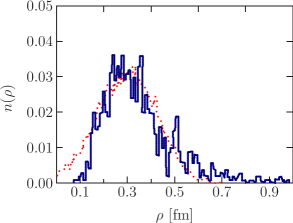
Figure 2: The instanton size distribution function $n(\rho)$. The dots correspond to the calculations in the framework of ILM, while the continuous lines correspond to the lattice simulations [16].

In what follows we will use a shorthand notation $\xi_{I},\xi_{\bar{I}}$ for the collective coordinates of the instantons and antiinstantons: the position in 4-dimensional Euclidean space $z_{I}$, the instanton size $\rho_{I}$ and the unitary SU$(N_{c})$ color orientation matrix $U_{I}$, which itself depends on $4N_{c}$ variables, where $N_{c}$ is the number of colors. Hereafter, sometimes we will drop the subscripts $I,\bar{I}$ for the sake of brevity, when this does not cause additional confusion.

There are two main parameters in ILM – the average instanton size $\bar{\rho}$ and the inter-instanton distance $R$. The latter describes the density of instanton media $N/V\equiv 1/R^{4}$, where $N$ is the total number of instantons. Phenomenologically this density is related to the gluon condensate as [9]

$$\frac{N}{V}\simeq\frac{1}{32\pi^{2}}\langle F_{\mu\nu}^{a}F_{\mu\nu}^{a}\rangle\simeq(200\,{\rm MeV})^{4}.$$ (1)

which allows to obtain an estimate $R\simeq 1\,{\rm fm}$.The instanton size $\rho$ effectively sets the scale, which controls the value of the renormalized strong coupling $\alpha_{s}$ [10, 11]. In one-loop approximation ( $\overline{{\rm MS}}$ scheme) we have

$$\frac{2\pi}{\alpha_{s}(\rho)}=b_{1}\ln\frac{1}{\Lambda_{\overline{MS}}\,\rho},\,\,\,b_{1}=\frac{11}{3}N_{c}-\frac{2}{3}N_{f}$$ (2)

where $N_{c}$ is the introduced earlier number of colors, and $N_{f}$ is the number of light flavors. At $1/\rho=600$ MeV, using $\Lambda_{\overline{MS}}=100$ MeV, we may obtain a rather large value$\alpha_{s}(\rho)=0.39.$

Due to conformal symmetry of classical QCD, a single instanton may have any size. However, due to quantum corrections, as we approach $\rho\Lambda_{\overline{MS}}\sim 1$, the semiclassical approximation becomes absolutely inapplicable. In the instanton-antiinstanton medium, due to mutual interactions, both parameters $R$ and $\rho$ are close to their average values $\bar{R}\approx 1$ fm, $\bar{\rho}\approx 0.33$ fm values, which were found by the application of Feynman variational method to this problem by Diakonov and Petrov [5] (see also reviews [3, 1, 2]), and further confirmed by the lattice simulations of the QCD vacuum [12, 13, 14, 15] (see Fig. 1). A detailed studies of the instanton size distribution $n(\rho)$ was made in [16], and is shown in Fig. 2, where the results in framework of ILM model are also given for comparison. We can see that at the relatively large values of instanton sizes $\rho\gtrsim R$, where more intensive overlapping of instantons might happen, the distribution function $n(\rho)$ is strongly suppressed. A rather narrow peak of the distribution is localized around $\rho\simeq 0.35$ fm, which corresponds to the average size $\bar{\rho}$. Therefore, for practical calculations we can disregard distribution of instantons by size, and effectively replace them all with average-size instantons. In what follows we will use this scheme and disregard possible corrections due to finite width of the distribution $n(\rho)$, assuming $\rho=\bar{\rho}$. The diluteness of the instanton gas and smallness of the packing fraction $\kappa=\bar{\rho}^{4}/R^{4}\sim 0.01$ justifies the use of simple sum-ansatz for the total instanton field $A(\xi)=\sum_{i}A_{i}(\xi_{i})$, which is expressed in terms of the single instanton solutions $A_{i}(\xi_{i})$ Using the typical values of the ILM parameters $R=1$ fm, $\bar{\rho}=1/3$ fm, we can estimate the QCD vacuum energy density, which takes the nonzero value, $\epsilon\approx-500\,{\rm MeV/fm^{3}}$ [1, 2].

Finally, we would like to mention that the large-size tail of the instanton distribution $n(\rho)$ becomes important in the confinement regime of QCD. Here in order to take instanton phenomena more accurately, we should replace Belavin-Polyakov-Schwarz-Tyupkin instantons by Kraan-vanBaal-Lee-Lu instantons [21, 22, 23] described in terms of dyons. In such a way, we get a natural extension of the instanton liquid model, the so-called liquid dyon model (LDM) [24, 25, 26]. This model allow to reproduce the confinement–deconfinement phases. The small size instantons in this approach can still be described in terms of their collective coordinates. For comparison, the average size of instantons in liduid dyon model is $\bar{\rho}_{{\rm LDM}}\approx 0.5\,{\rm fm}$ [24, 25, 26], slightly larger than the above-mentioned estimate in the instanton liquid model.

II Light quarks in ILM

As discussed earlier in Introduction, one of the most prominent achievements of the instanton vacuum model is the correct description of the spontaneous breaking of the chiral symmetry (SBChS), which is responsible for properties of most hadrons and nuclei  [17] and is due to specific nonperturbative properties of QCD vacuum. In the instanton picture SBChS occurs due to the delocalization of the single-instanton quark zero modes in the instanton medium.

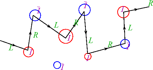
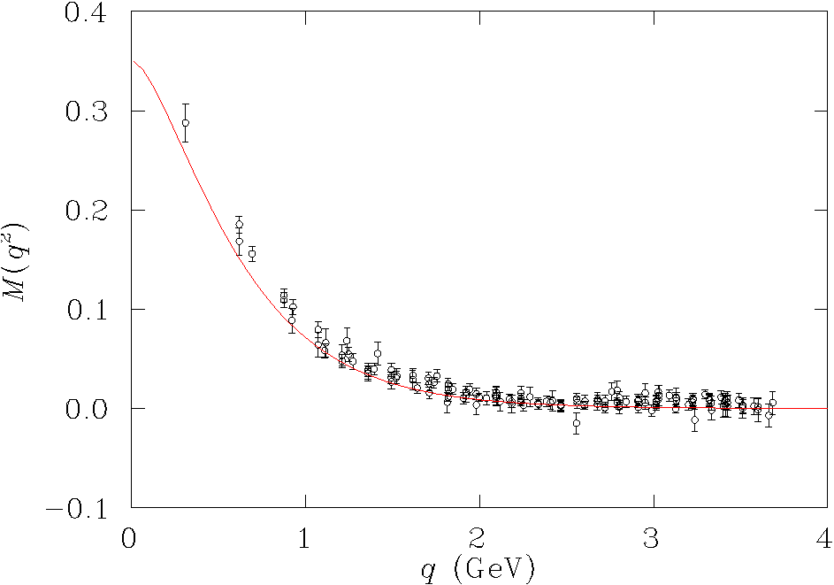
Figure 3: Left plot: Schematic illusration of quark rescatterings in the field of individual instantons and antinistantons which leads to SBChS. Right plot: Comparison of the dynamical quark mass $M_{q}(q)$ from ILM and lattice calculations [44].

The integration over the light quark degrees of freedom in the partition function leads to the determinant of the light quark propagator $S$ evaluated in the background field of instanton liquid. We may split this determinant into the low- and high-frequency parts according ${\rm Det}={\rm Det}_{\mathrm{low}}{\rm Det}_{\mathrm{high}}$. The high-energy part ${\rm Det}_{\mathrm{high}}$ is responsible mainly for the perturbative coupling renormalization, for this reason in what follows we disregard it and concentrate on the evaluation of the nonperturbative contribution ${\rm Det}_{\mathrm{low}}$, which is responsible for the low-energy domain. As was suggested in  [10, 18, 19, 20], we may start evaluation with the zero-mode approximation for the light quark propagator of a quark in the field of the isolated $i$-th instanton,

$$S_{i}=\frac{1}{\hbox to0.0pt{/\hss}{p}+\hbox to0.0pt{/\hss}{A}_{i}+im}=\frac{1}{\hbox to0.0pt{/\hss}{p}}+\frac{|\Phi_{i,0}\rangle\langle\Phi_{i,0}|}{im}.$$ (3)

While this approximation is good for small values of the current quark mass $m$, we need to extend it beyond the chiral limit as proposed in our previous works  [29, 30, 31, 32, 33, 35] as follows:

$$S_{i}=S_{0}+S_{0}\hbox to0.0pt{/\hss}{p}\frac{|\Phi_{0i}\rangle\langle\Phi_{0i}|}{c_{i}}\hbox to0.0pt{/\hss}{p}S_{0},$$ (4)

where

$$c_{i}=-\langle\Phi_{0i}|\hbox to0.0pt{/\hss}{p}S_{0}\hbox to0.0pt{/\hss}{p}|\Phi_{0i}\rangle=im\langle\Phi_{0i}|S_{0}\hbox to0.0pt{/\hss}{p}|\Phi_{0i}\rangle=im\langle\Phi_{0i}|\hbox to0.0pt{/\hss}{p}S_{0}|\Phi_{0i}\rangle.$$ (5)

The approximation given in Eq.(4) allows us to get correct projection of $S_{i}$ on the would-be zero-modes in presence of finite quark mass $m$,

$$S_{i}|\Phi_{0i}\rangle=\frac{1}{im}|\Phi_{0i}\rangle,\,\,\,\langle\Phi_{0i}|S_{i}=\langle\Phi_{0i}|\frac{1}{im}.$$ (6)

As we mentioned earlier, in dilute liquid approximation the instanton ensemble might be represented as a superposition of gluonic fields of individual instantons, for this reason we can represent the total quark propagator ${S}$ in the presence of the whole instanton ensemble $A$ in terms of the quark propagators of individual instantons. Physically, this corresponds to resummation of a multi-scattering series, shown schematically in the left panel of the Figure 3. Making a few technical steps [35], we may represent this determinant in terms of the low-energy contributions of individual instantons. In what follows we will focus on evaluation of the partition function, which depends on the external quark sources $\eta,\bar{\eta}$, for this reason from now on we will incorporate them in our consideration. The fermionized representation of the low-frequencies light quark determinant in the presence of these quark sources $\bar{\eta},\,\eta$ is given by

$${\rm Det}_{{\rm low}}\exp\left(-\eta^{+}S\eta\right)=$$

$$=\int\prod_{f}D\psi_{f}D\psi_{f}^{\dagger}\exp\int\sum_{f}\left(\psi_{f}^{\dagger}(\hat{p}\,+\,im_{f})\psi_{f}+\psi_{f}^{\dagger}\eta_{f}+\eta_{f}^{+}\psi_{f}\right)\prod_{f}\prod_{\pm}^{N_{\pm}}V_{\pm,f}[\psi^{\dagger},\psi,\xi_{\pm}],$$ (7)

where the vertices

$$V_{\pm,f}[\psi^{\dagger},\psi,\xi_{\pm}]=i\int d^{4}x\left(\psi_{f}^{\dagger}(x)\,\hat{p}\Phi_{\pm,0}(x;\xi_{\pm})\right)\int d^{4}y\left(\Phi_{\pm,0}^{\dagger}(y;\xi_{\pm})(\hat{p}\,\psi_{f}(y)\right)$$ (8)

correspond to interaction of the light quarks with individual instantons.

The averaging over the collective coordinates $\xi_{i,\pm}$ in (7, 8) is straightforward, since the low density of the instanton liquid allows to average over positions and orientations of the individual instantons independently from each other. This process leads to the light quark partition function $Z[\eta,\eta^{\dagger}]$. We see that

$$Y_{\pm}[\psi^{\dagger},\psi]=\int d\xi_{\pm}\prod_{f}V_{\pm,f}[\psi^{\dagger},\psi,\xi_{\pm}]$$ (9)

is instanton-generated light quarks $2N_{f}$-legs interaction represented in Fig. 4.

Figure 4: Instanton-generated light quarks interaction $W_{\pm}[\psi^{\dagger},\psi]$ with $2N_{f}$-legs.

The nonlocal form-factor in the interaction vertex (8, 9) is completely defined by the quark zero-mode. For further evaluations it is convenient to raise the vertices $Y_{\pm}$ into the argument of exponent, using the so-called exponentiation with the help of Stirling-like formula

$$Y_{\pm}^{N_{\pm}}=\int d\lambda_{\pm}\exp(N_{\pm}\ln\frac{N_{\pm}}{\lambda_{\pm}}-N_{\pm}+\lambda_{\pm}Y_{\pm}),$$ (10)

where $\lambda_{\pm}$ play a role of the dynamical coupling constant, defined by saddle-point condition at the integral (10). The validity of the formula (10) is controlled by the large number of instantons $N_{\pm}\gg 1$. The partition function of the light quarks (7) at $N_{f}=1$ and $N_{\pm}=N/2$ is exactly given by

$$Z\left[\eta,\eta^{\dagger}\right]=e^{-\eta^{+}\left(\hat{p}\,+\,i(m+M(p))\right)^{-1}\eta}\exp\left[{\rm Tr}\ln\left(\hat{p}\,+\,i(m+M_{q}(p))\right)+N\ln\frac{N}{2\lambda}-N\right],$$ (11)

$$N={\rm Tr}\frac{iM_{q}(p)}{\hat{p}\,+\,i(m+M_{q}(p))},\,\,\,M_{q}(p)=M_{q}F^{2}(p),\,\,\,\,M_{q}=\frac{\lambda}{N_{c}}(2\pi\rho)^{2},$$ (12)

where the form-factor $F(p)$ is related to the Fourier-transform of the zero-mode. The dynamical quark mass $M_{q}(p)$ defined in the Eq. (12) is the instanton-induced nonperturbative contribution to the dynamical quark mass, whose dependence on the quark momentum is shown in the right panel of the Figure 3. From this equation we can see that it simultaneously determines the strength of the light quark-instanton interaction, which is parametrically given by $M_{q}\sim\kappa^{1/2}\rho^{-1}$. Its numerical value might be found solving the first equation in (12), and at typical values of $\bar{\rho}\approx 1/3$ fm, $R\approx 1$ fm we may get $M_{q}\approx 360$ MeV. For number of flavors $N_{f}>1$, using the saddle-point approximation, in the leading order we may get the same value of $M_{q}$.

II.1 Light mesons effective action at $N_{f}=2$ with nonleading order (NLO) contributions
and Chiral Perturbation Theory (ChPT) couplings

The partition function in the presence of external fields provides a straightforward way for the calculations of various correlators. This function for the two light flavors has been evaluated in the framework of ILM in our previous paper [34]. We found that the light quarks partition function $Z[v,a,s,p,m]$ in the presence of external vector $v_{\mu}$, pseudovector $a_{\mu}$, scalar $s$ and pseudoscalar $p$ fields is given by:

$$\tilde{Z}[v,a,s,p,m]=\int\prod_{f}D\psi_{f}D\psi_{f}^{\dagger}\exp\left(\int d^{4}x\sum_{f,g}\psi_{f}^{\dagger}(\hat{p}\,+\,\hat{V}\,+\,im)_{fg}\psi_{g}\right)\prod_{\pm}^{N_{\pm}}\tilde{Y}_{\pm}[\psi^{\dagger},\psi],$$

$$\tilde{Y}_{\pm}[\psi^{\dagger},\psi]=\int d\xi_{\pm}\prod_{f}\tilde{V}_{\pm,f}[\psi^{\dagger},\psi],$$ (13)

where

$$\tilde{V}_{\pm}[\psi^{\dagger},\psi]=\int d^{4}x\left(\psi^{\dagger}(x)\,\bar{L}^{-1}(x,z_{\pm})\,\hat{p}\Phi_{\pm,0}(x;\xi_{\pm})\right)\int d^{4}y\left(\Phi_{\pm,0}^{\dagger}(y;\xi_{\pm})(\hat{p}\,L^{-1}(y,z_{\pm})\psi(y)\right),$$ (14)

$\tilde{Y}_{\pm}[\psi^{\dagger},\psi]$ is the t’Hooft-like non-local interaction term with $N_{f}$ pairs of quark legs in the presence of the external fields, and $L_{i}$ is the gauge connection defined as a path-ordered exponent

$$L_{i}(x,z_{i})={\rm P}\exp\left(i\int_{z_{i}}^{x}dy_{\mu}(v_{\mu}(y)+a_{\mu}(y)\gamma_{5})\right),\,\,\,\bar{L}_{i}(x,z_{i})=\gamma_{4}L_{i}^{\dagger}(x,z_{i})\gamma_{4};$$ (15)

the variable $z_{i}$ denotes the instanton or antiinstanton position. After integration over collective coordinates and exponentiation, the partition function may be reduced to the form :

$$\tilde{Z}=\int d\lambda_{+}d\lambda_{-}D\psi^{\dagger}D\psi\exp\left[-\left(N_{\pm}\ln\frac{K}{\lambda_{\pm}}-N_{\pm}+\psi^{\dagger}(i\hat{\partial}+\hat{V}+im)\psi+\lambda_{\pm}\tilde{Y}_{2}^{\pm}\right)\right];$$

$$\tilde{Y}_{2}^{\pm}=\frac{2N_{c}-1}{2N_{c}(N_{c}^{2}-1)}\left(\det_{f}J^{\pm}+\frac{1}{8N_{c}-4}\det_{f}J_{\mu\nu}^{\pm}\right),$$

$$J^{\pm}=\psi^{\dagger}\bar{L}\frac{1\pm\gamma_{5}}{2}L^{-1}\psi,\,\,J_{\mu\nu}^{\pm}=\psi^{\dagger}\bar{L}\sigma_{\mu\nu}\frac{1\pm\gamma_{5}}{2}L^{-1}\psi,$$ (16)

where the determinant is taken over the (implicit) flavor indices, and $K$ is some inessential constant introduced to make the argument of logarithm dimensionless. From (16) we can clearly see that the contribution of the tensor terms is just a $1/N_{c}$-correction. For the sake of simplicity we will postpone consideration of the tensor terms contribution and concentrate on the first term in (16). The expression $\det_{f}J^{\pm}$ includes a product of $2N_{f}$ quark operators, which might be represented in a more convenient form using the bosonization of the interaction term $H_{\pm}[\psi^{\dagger},\psi]$. For the sake of simplicity we will consider only the $N_{f}=2$ case, for which bosonization is an exact procedure, and take $N_{+}=N_{-}$, as discussed before. We get for the partition function

$$\tilde{Z}[v,a,s,p,m]=\int d\lambda D\Phi D\psi^{\dagger}D\psi$$

$$\times\exp\left[N\ln\frac{K}{\lambda}-N+\int dx\left(-2\Phi^{2}+\psi^{\dagger}(\hat{p}+\hat{v}+\hat{a}\gamma_{5}+im+i\frac{(2\pi\rho)^{2}\lambda^{0.5}}{2g}\bar{L}\hat{F}\Phi\cdot\Gamma\hat{F}L)\psi\right)\right]$$ (17)

or, integrating over fermions,

$$\tilde{Z}[v,a,s,p,m]=\int d\lambda D\Phi e^{-\tilde{S}[\lambda,\Phi,v,a,s,p,m]},$$ (18)

where

$$\tilde{S}[\lambda,\Phi,v,a,s,p,m] = 2\int dx\,\Phi^{2}+{\rm Tr}\ln\left(\frac{\hat{p}+\hat{v}+\hat{a}\gamma_{5}+im+i\frac{(2\pi\rho)^{2}\lambda^{0.5}}{2g}\bar{L}\hat{F}\Phi\cdot\Gamma\hat{F}L}{\hat{p}+\hat{v}+\hat{a}\gamma_{5}+im}\right)+N\ln\frac{K}{\lambda}-N$$ (19)

and $g^{2}=\frac{(N_{c}^{2}-1)2N_{c}}{2N_{c}-1}$ is a color factor;, matrices $\Gamma=\{1,\gamma_{5},i\vec{\tau},i\vec{\tau}\gamma_{5}\},$ and we will use notations for the components of the field $\Phi$ in front of them $\Phi=\{\Phi_{0},\vec{\Phi}\}=\{\sigma,\eta,\vec{\sigma},\vec{\phi}\}$, with $\Phi^{2}=\Phi_{0}^{2}+\vec{\Phi}^{2}=\sigma^{2}+\eta^{2}+\vec{\sigma}^{2}+\vec{\phi}^{2}$. Notice that in (17) in contrast to the NJL model the coupling constant $\lambda$ is not a parameter of the action but it is defined by saddle-point condition in the integral (17). The partition function (17) is invariant under local flavour rotations due to the gauge links $L$ in the interaction term $\tilde{V}_{\pm,f}[\psi^{\dagger},\psi]$. However, instead of the explicit violation of the gauge symmetry due to the zero-mode approximation (3,4), we have unphysical dependence of the effective action on the choice of the path in the gauge link $L$. In our evaluations we used the simplest straight-line path, though there is no physical reasons why the other choices should be excluded. In the low-energy region we demonstrated explicitly that the path dependence drops out.

We will start the calculations of the partition function assuming for simplicity zero external currents, and will apply it to evaluation of the quark condensate $\langle\bar{q}q\rangle$, which is one of the main manifestations of the SChSB. Technically, it happens due to the quark-quark interaction term (13), which leads to the strong attraction in the channels with vacuum (and pion) quantum numbers. As a consequence, the vacuum of the theory has a nonzero vacuum expectation $\sigma$ of scalar-isoscalar component of meson fields $\Phi$ and quark condensate $\langle\bar{q}q\rangle$. For evaluation of the partition function $Z[m]$ it is very convenient to use the formalism of the effective action [42, 43] $\Gamma_{eff}[m,\lambda,\Phi]$, which is defined as

$$\tilde{Z}[m]=\int d\lambda\tilde{Z}[m,\lambda]=\int d\lambda\exp(-\Gamma_{eff}\left[m,\lambda,\Phi\right]),$$ (20)

where the field $\Phi$ is the solution of the vacuum equation

$$\frac{\partial\Gamma_{eff}[m,\lambda,\Phi]}{\partial\Phi}=0,$$ (21)

and implicitly depends on $\lambda$, i.e. $\Phi=\Phi(\lambda)$. In view of (21), the definition (20) is equivalent to the definition via Legendre transformation of partition function, which is conventionally used in the Quantum Field Theory. The only nonzero vacuum meson field which might have nonzero vacuum expectation is a condensate $\Phi=\sigma$. In view of the translation invariance of the effective action $\Gamma_{eff}[m,\lambda,\Phi]$, on vacuum cconfigurations the latter may be replaced with effective potential $V_{eff}[m,\lambda,\sigma]$.

In absence of quantum (loop) corrections, the effective action just coincides with the action (19). Making expansion of the mesonic field near its vacuum value, $\Phi\approx\sigma+\Phi^{\prime}$, and integrating over the fluctuations, we get for the meson loop correction to the effective action

$$\Gamma_{eff}^{mes}[m,\lambda,\sigma]=\frac{1}{2}{\rm Tr}\ln\left(4\delta_{ij}-\frac{1}{\sigma^{2}}{\rm Tr}\frac{M_{q}(p)}{\hat{p}+i(m+M_{q}(p))}\Gamma_{i}\frac{M_{q}(p)}{\hat{p}+i(m+M_{q}(p))}\Gamma_{j}\right).$$ (22)

where $M_{q}(p)$ is the dynamical quark mass defined in (12). Formally, meson loops lead to NLO corrections which are suppressed as $\mathcal{O}\left(1/N_{c}\right)$  in the limit $N_{c}\to\infty$. We found as result of the calculations These corrections affect all physical observables, and for example, for the dynamical mass instead of (12) we get significantly more sophisticated equation whose solution yields

$$M(m)=0.36-2.36\,m-\frac{m}{N_{c}}(0.808+4.197\ln m)$$ (23)

The essential feature of Eq. (23) is the presence of the chiral logs originated from pion loops, as expected from chiral perturbation theory [45]. The accuracy of these solutions is ${\cal O}\left(m^{2},\frac{1}{N_{c}^{2}}\right).$ Left plot in Fig.5 represents the $M(m)$-dependence obtained from Eq. (21) with account of $\mathcal{O}(1/N_{c})$ meson loops corrections. For the sake of comparison, we also plotted the lattice data from [44].

Figure 5: Left plot: The $m$-dependence of the dynamical quark mass $M$. The solid curve is the exact numerical solution (23) of the vacuum Eqs. (21). The dashed curve is the solution obtained by the iterations ($1/N_{c}$-expansion) with the same accuracy. Data points are from [44]. Notice that the scale of the lattice data is $1.64\,{\rm GeV}$, not $\rho^{-1}\approx 0.6\,{\rm GeV}$. The discrepancy may be attributed to the scales difference. Right plot: The $m$-dependence of the quark condensate $-\langle\bar{q}q\rangle$. The long-dashed curve is the leading-order (LO) result $-<{\bar{q}q}>_{LO}$, The dot-dashed line represents LO in $1/N_{c}$-expansion result. The short-dashed curve is the NLO contribution $-<{\bar{q}q}>_{NLO}$, the solid curve is the total contribution $-<{\bar{q}q}>_{LO+NLO}$.

The quark condensate $\langle\bar{q}q\rangle$ can be extracted directly from the effective action as

$$\langle\bar{q}q\rangle=\frac{1}{2}\frac{\partial\Gamma_{eff}}{\partial m}$$ (24)

Evaluation of (24) gives

$$-\langle\bar{q}q\rangle(m)=\left[\left(0.00497-0.0343\,m\right)\,N_{c}+\right.$$ (25)

$$\left.+\left(0.00168-0.0494\,m-0.0580\,m\,\ln m\right)\right]\left[{\rm GeV}^{3}\right]+{\cal O}\left(m^{2},\frac{1}{N_{c}}\right)$$

The $\langle\bar{q}q\rangle(m)$-dependence is depicted in the right panel of the Fig. 5. We can see again that due to the chiral logarithm the $m$-dependence is not linear, and meson loops change drastically the $m-$dependence of the quark condensate.

The extension of this procedure in background of weak external sources $v,a,s,p$ is straightforward and might be done perturbatively. The correlators of axial-vector and pseudoscalar currents, which are important for the Chiral Perturbation Theory ($\chi$PT) [45], can be extracted from the Eq.(18) by taking into account respective external axial-vector and pseudoscalar sources. Using the action (19) and taking into account the loop corrections as described earlier, we may obtain the correlators of axial currents, which allow to extract the $m$-dependence of the pion decay constant $F_{\pi}$ and pion mass $M_{\pi}$,

$$F_{\pi}^{2}=N_{c}\left(\left(2.85-\frac{0.869}{N_{c}}\right)-\left(3.51+\frac{0.815}{N_{c}}\right)m-\frac{44.25}{N_{c}}\,m\,\ln m+{\cal O}\left(m^{2}\right)\right)\cdot 10^{-3}\;\left[{\rm GeV}^{2}\right]$$ (26)

where $m$ is given in GeV, the constant in front of ${\cal O}(m^{0})$ contribution is given in ${\rm GeV}^{2}$, and the constant in front of ${\cal O}(m)$ term is given in ${\rm GeV}$. The $F_{\pi}(m)$-dependence is shown in the left panel of the Fig. 6. For the sake of comparison, we also plotted the value $F_{\pi,0}$ which we would get using LO formulae with the mass $M_{0}(m)$. Recall that the value $F_{\pi}(m=0)=88\,{\rm MeV}$, as well as $<{\bar{q}q(m=0)}>=(255\,MeV)^{3}$, was used as the input in order to fix the parameters $(\rho,\,R)$. The comparison between the solid curve and the long-dashed one shows that the effect of the NLO-corrections grows with $m$ and is about $40\%$ at $m=0.1\,{\rm GeV}$. Similar calculations for the pion mass $M_{\pi}(m)$ yield

$$M_{\pi}^{2}=m\left(\left(3.49+\frac{1.63}{N_{c}}\right)+m\left(15.5+\frac{18.25}{N_{c}}+\frac{13.5577}{N_{c}}\ln m\right)+{\cal O}(m^{2})\right)$$ (27)

in the next-to leading order. The $M_{\pi}(m)$-dependence of the pion mass is shown in the right panel of Fig.  6. For the sake of comparison, we also plotted the value $M_{\pi,0}$. which one would get using LO formulae with the mass $M_{0}(m)$. Altogether, for this observables the NLO-corrections turn out to be small.

Figure 6: Left panel: The $m$-dependence of the pion decay constant $F_{\pi}$. The long-dashed curve is the LO contribution, the short-dashed curve is the NLO contribution, the solid curve is the total LO+NLO contribution. The dot-dashed line represents the leading-order in $1/N_{c}$-expansion result. Right panel: The $m$-dependence of the pion mass $M_{\pi}$. The long-dashed curve is the LO contribution, the short-dashed curve is the NLO contribution, the solid curve is the total LO+NLO contribution. The dot-dashed line represents the lowest order in $1/N_{c}$-expansion result.

These results are essential and allow for the extraction of the low-energy constants of Chiral Perturbation Theory (ChPT), matching the expected $m$-dependence in that theory with $m$-dependence found in Instanton Liquid Model. . According to [45], the low-energy constants $\bar{l}_{i}$ of the chiral lagrangian appear in some of the ${\cal O}(m)$-corrections to physical quantities, e.g.

$$M_{\pi}^{2}=m_{\pi}^{2}\left(1-\frac{m_{\pi}^{2}}{32\pi^{2}F^{2}}\bar{l}_{3}+{\cal O}(m_{\pi}^{4})\right),\,\,F_{\pi}^{2}=F^{2}\left(1+\frac{m_{\pi}^{2}}{8\pi^{2}F^{2}}\bar{l}_{4}+{\cal O}(m_{\pi}^{4})\right),$$ (28)

where $M_{\pi},F_{\pi}$ are the pion mass and decay constants, $m_{\pi}^{2}=2\,m\,B$ and $B,F$ are the phenomenological parameters of the chiral lagrangian. Using our results (26, 27), we can obtain

$$F^{2}=0.00284777N_{c}-0.000868917+{\cal O}\left(\frac{1}{N_{c}}\right),\,\,\,B=1.7467+\frac{0.8183}{N_{c}}+{\cal O}\left(\frac{1}{N_{c}^{2}}\right)$$ (29)

$$\bar{l}_{3}=0.0738267-1.14251\,N_{c}-0.999\,\ln\left(\frac{m}{{\rm GeV}}\right)+{\cal O}\left(\frac{1}{N_{c}}\right)$$ (30)

$$\bar{l}_{4}=-0.0793814\,N_{c}+0.0187608-1.000\,\ln\left(\frac{m}{{\rm GeV}}\right)+{\cal O}\left(\frac{1}{N_{c}}\right)$$ (31)

which gives numerically

$$F=88\,{\rm MeV},\;B=2.019\,{\rm GeV},\;\bar{l}_{3}=1.84,\;\bar{l}_{4}=4.98$$ (32)

for current mass $m=0.0055\,\,{\rm GeV}$; the corresponding values of the pion mass and decay constant are given by $M_{\pi}=0.142\,\,{\rm GeV}$, $F_{\pi}=0.0937\,\,{\rm GeV}$. We need to mention that the values of $F,-\langle{\bar{q}q(m=0)}\rangle=-F^{2}B$ in (32) were taken as input when we fixed the parameters $\bar{\rho},\,R$. Our results for $\bar{l}_{3},\bar{l}_{4}$ are in fair agreement with the phenomenological estimates [46, 47] and lattice predictions [48, 49] given in Table 1.

	ChPT	MILC	Del Debbio	ETM	Our
	[50, 45, 47]	[51]	et. al. [49]	[52]	prediction
$\bar{l}_{3}$	$2.9\pm 2.4$	$0.6\pm 1.2$	$3.0\pm 0.5$	$3.62\pm 0.12$	$1.84$
$\bar{l}_{4}$	$4.4\pm 0.2$	$3.9\pm 0.5$	—	$4.52\pm 0.06$	$4.98$

Table 1: Estimates and predictions of the low-energy constants $\bar{l}_{3},\,\bar{l}_{4}$. The first column contains phenomenological estimates, the next three columns are lattice results from different collaborations, the last column contains our results. The first four columns of the table are taken from [47].

Notice that in (30 - 32) we keep ${\cal O}(N_{c},N_{c}^{0})$-terms and drop NNLO terms ${\cal O}(1/N_{c})$ in agreement with our general framework. Without such expansion we would get

$$\bar{l}_{3}=0.28, \bar{l}_{4}=4.28.$$ (33)

Also, other similar ChPT low energy parameters were successfully calculated within ILM [32, 35, 36]. So, ILM is reliable nonperturbative QCD tool for low energy light quarks processes.

III Heavy and light quarks systems in ILM

As we found above, the strength of instanton-light quark interaction is fairly large and induces strong interaction between light quarks, leading to formation of almost massless pions and nonzero quark condensate, in accordance with expectations of SBChS. We have seen that the physics in this domain is closely related to the low-energy behaviour of the light quark propagator, which is dominated by its zero mode. On the other hand, heavy quarks dynamics is controlled mainly by their heavy masses $M_{Q}$, and we expect rather weak instanton-heavy quark interaction. Nevertheless, we expect essential influence of instantons for the heavy-light quarks systems.

III.1 The strength of heavy-quark-instanton interaction

First, we simplify the problem by taking an infinitely heavy quark, which interacts only through the fourth components of instantons $A_{4}$. Hereafter, we follow the definitions given in Ref. [74], i.e. $\theta$ is inverse of differentiation operator $\theta^{-1}=d/dt$ and $\langle t|\theta|t^{\prime}\rangle=\theta(t-t^{\prime})$ is a step-function. For the sake of convenience, we also redefine the gluonic field as $A\equiv iA_{4}$. Accordingly, the heavy quark $Q$ and antiquark $\bar{Q}$ Lagrangians can be expressed as

$$L_{Q}=Q^{+}(\theta^{-1}-gA+...)Q,\,\,\,L_{\bar{Q}}=\bar{Q}^{+}(\theta^{-1}-g\bar{A}+...)\bar{Q},$$ (34)

where the dots denote the next order in the inverse of heavy quark mass terms. In terms of SU($N_{c}$) generators, the fields $A$ and $\bar{A}$ are given as $A=A_{a}\lambda_{a}/2$ and $\bar{A}_{a}=A_{a}\bar{\lambda}_{a}/2$, where $\bar{\lambda}_{a}=-\lambda_{a}^{{\rm T}}$ (here ‘T’ means the transposition). In our calculations we may neglect the virtual processes $Q\rightarrow QQ\bar{Q}$ corresponding to the heavy quark loops, which effectively means the heavy quark determinant equals to unity. The functional space of heavy quarks $Q$ is not overlapping with the functional space of heavy antiquarks $\bar{Q}$ and, consequently, the total functional space is a direct product of $Q$ and $\bar{Q}$ spaces.

After averaging over instantons collective coordinates, the propagator of the infinitely heavy quark $Q$ in ILM is given by

$${w}=\!\int\!D\xi\frac{1}{\theta^{-1}-gA(\xi)}.$$ (35)

In order to integrate over instanton collective coordinates $\xi_{i}$ one can now apply Pobylitsa’s equation from Ref. [74] and follow their solution in the lowest order in packing parameter $\kappa$,

$$w^{-1}=\theta^{-1}-\sum_{i}^{N}\int d\xi_{i}\theta^{-1}\left(\frac{1}{\theta^{-1}-gA_{i}(\xi_{i})}-\theta\right)\theta^{-1}+O(\kappa^{2}).$$ (36)

The calculations of the matrix element of the second term in the right-hand side of Eq. (36) provides the direct ILM heavy quark mass shift $\Delta M_{Q}^{{\rm dir}}$ with corresponding order ${\cal O}(\kappa)$. We note that the direct instanton contribution to the heavy quark mass $\Delta M_{Q}^{{\rm dir}}$ was calculated first in Ref. [74]. Numerically, one can estimate

$$\Delta M_{Q}^{{\rm dir}}\simeq 70\,{\rm MeV}\sim\kappa\rho^{-1}.$$ (37)

This value controls the strength of heavy-quark-instanton interaction, which is much weaker than that of the light quarks, in agreement with expectations based on heavy quark mass limit.

III.2 Heavy and light quarks interactions in ILM

It is obvious that the light quarks affect the integration in (35) via the contributions of the light quark determinant. For our aim it is useful to take into account light quarks sources, Eq. (7), and extend the Eq. (35) in the form

$$w=\int\prod_{f}D\psi_{f}D\psi_{f}^{\dagger}\exp\int\sum_{f}\left(\psi_{f}^{\dagger}(\hat{p}\,+\,im_{f})\psi_{f}\right)\prod_{\pm}^{N_{\pm}}H_{\pm}[\psi^{\dagger},\psi]w[\psi,\psi^{\dagger}],$$ (38)

$$H_{\pm}[\psi^{\dagger},\psi]=\int d\xi_{\pm}\prod_{f}V_{\pm,f}[\psi^{\dagger},\psi,\xi_{\pm}],$$ (39)

$$w[\psi,\psi^{\dagger}]=\left\{\prod_{\pm}^{N_{\pm}}H_{\pm}[\psi^{\dagger},\psi]\right\}^{-1}\!\!\!\int\prod_{\pm}^{N_{\pm}}d\xi_{\pm}\left\{\prod_{\pm}^{N_{\pm}}V_{\pm,f}[\psi^{\dagger},\psi,\xi_{\pm}]\right\}\left(\theta^{-1}-\sum_{i}A_{i}\right)^{-1}.$$ (40)

The measure of the integration over $\xi_{\pm}$ in the Eq. (40) with and without light quark factor $\prod_{f}V_{\pm,f}[\psi^{\dagger},\psi]$ has the same structure as a product of independent integrations over the instanton collective coordinates $\xi_{\pm}$. Then, we may extend the derivation of the Pobylitca equations [74, 59] and solve them in the dilute approximation as

$$w^{-1}[\psi,\psi^{\dagger}]=\theta^{-1}-\frac{N}{2}\sum_{\pm}\frac{1}{H_{\pm}[\psi^{\dagger},\psi]}\Delta_{Qq,\pm}[\psi^{\dagger},\psi]+O(\kappa^{2}),$$ (41)

where, defining the heavy quark propagator in the single (anti)instanton field as $w_{\pm}=(\theta^{-1}-A_{\pm})^{-1}$, we have

$$\Delta_{Qq,\pm}[\psi^{\dagger},\psi]=\int d\xi_{\pm}\prod_{f}V_{\pm,f}[\psi^{\dagger},\psi,\xi_{\pm}]\theta^{-1}(w_{\pm}[\xi_{\pm}]-\theta)\theta^{-1}.$$ (42)

The last expression represents the interactions of heavy $Q$ and $N_{f}$ light quarks $q$ generated by instantons as (see Fig. 7)

$$S_{Qq}=-\lambda\sum_{\pm}\int Q^{\dagger}\Delta_{Qq,\pm}[\psi^{\dagger},\psi]Q.$$ (43)

Figure 7: Instanton generated heavy $Q$ and $N_{f}$ light $q$ quarks interaction.

It is straightforward to see that without light quarks factors $V_{\pm,f}[\psi^{\dagger},\psi,\xi_{\pm}]$, the Eq. (42) reduces to the second term of Eq. (36), which gives the direct ILM contribution to the heavy quark mass $\Delta M_{Q}^{{\rm dir}}$. It is obvious that the light quark pairs are produced in color singlet or color octet states. Let us consider $N_{f}=2$ colorless light quark pairs. These states are represented by mesons, and we’ll focus on the lightest of them, pions, as shown in Fig. 8.

Figure 8: Instanton generated emission of 2 pions by heavy $Q$ quark.

Technically, it can be done by bosonization method (see subsection II.1 for details). The corresponding amplitude of the emission of pions will have a form [39]

$$A_{Q\pi}=-F_{\pi Q}^{2}\int\frac{d^{4}x}{(2\pi)^{4}}e^{-ipx}{\rm tr}_{f}\partial_{\mu}U(x)\partial_{\mu}U^{+}(x)\Delta M_{Q}^{{\rm dir}}R^{4}F_{Q}(p),\,\,F_{Q}(p)=\frac{J_{0}(|\vec{p}|\rho)}{J_{0}(0)}.$$ (44)

where $J_{0}(|\vec{p}|\rho)$ is a Bessel function, and

$$F_{\pi Q}^{2}=2N_{c}\int\frac{d^{4}p}{(2\pi)^{4}}\frac{M^{2}(p)p^{2}}{(p^{2}+M^{2}(p))^{3}},$$ (45)

where $M(p)$ is the dynamical light quark mass. At the values of ILM parameters $\rho=1/3\,{\rm fm},\,\,\,R=1\,{\rm fm}$ one can get $F_{\pi Q}=0.6F_{\pi}$. Here the pion decay constant value in LO accordingly Eq. (29) is given by $F_{\pi}=92.4\,{\rm MeV}$. The integration over $x$ in Eq. (44) gives the $\delta$-function which reflects the energy-momentum conservation.

III.3 Heavy quarkonium and light quarks interactions in ILM

Now we will consider in ILM the $Q\bar{Q}$ correlator with the account of light quarks, which is defined as

$$\langle 0|T(Q^{\dagger}(t_{2}^{\prime},\vec{x}_{2})\bar{Q}^{\dagger}(t_{1}^{\prime},\vec{x}_{1}))\bar{Q}(t_{2},\vec{x}_{2})Q(t_{1},\vec{x}_{1})|0\rangle=\int D\psi_{f}D\psi_{f}^{\dagger}\left\{\prod_{\pm}^{N_{\pm}}H_{\pm}[\psi^{\dagger},\psi]\right\}$$

$$\times\exp\left(\int\sum_{f}\psi_{f}^{\dagger}(\hat{p}+im_{f})\psi_{f}\right)\langle t_{1}^{\prime},\vec{x}_{1};t_{2}^{\prime},\vec{x}_{2}|W[\psi,\psi^{\dagger}]|t_{1},\vec{x}_{1};t_{2},\vec{x}_{2}\rangle$$ (46)

where

$$\langle t_{1}^{\prime},\vec{x}_{1};t_{2}^{\prime},\vec{x}_{2}|W[\psi,\psi^{\dagger}]|t_{1},\vec{x}_{1};t_{2},\vec{x}_{2}\rangle=\left\{\prod_{\pm}^{N_{\pm}}H_{\pm}[\psi^{\dagger},\psi]\right\}^{-1}\int D\xi\left\{\prod_{\pm}^{N_{\pm}}\prod_{f}V_{\pm,f}[\psi_{f}^{\dagger},\psi_{f},\xi_{\pm}]\right\}$$ (47)

$$\times\langle t_{1}^{\prime},\vec{x}_{1}|\left(\theta^{-1}-\sum_{i}A_{i}^{(1)}\right)^{-1}|t_{1},\vec{x}_{1}\rangle\otimes\langle t_{2}^{\prime},\vec{x}_{2}|\left(\theta^{-1}-\sum_{i}\bar{A}_{i}^{(2)}\right)^{-1}|t_{2},\vec{x}_{2}\rangle$$

$${\rm and} \langle t_{1}^{\prime},\vec{x}_{1}|\left(\theta^{-1}-\sum_{i}A_{i}^{(1)}\right)^{-1}|t_{1},\vec{x}_{1}\rangle\otimes\langle t_{2}^{\prime},\vec{x}_{2}|\left(\theta^{-1}-\sum_{i}\bar{A}_{i}^{(2)}\right)^{-1}|t_{2},\vec{x}_{2}\rangle$$ (48)

$$= \left[T\exp\left(ig\int_{t_{1}^{\prime}}^{t_{1}}d\tau_{1}\sum_{i}A_{i,4}(\xi,\vec{x}_{1},\tau_{1})\right)\right]\left[T\exp\left(ig\int_{t_{2}^{\prime}}^{t_{2}}d\tau_{2}\sum_{i}\bar{A}_{i,4}(\xi,\vec{x}_{2},\tau_{2})\right)\right],$$

where $\otimes$ is a tensor product and the fields $A_{i}^{(1)}$ and $\bar{A}_{i}^{(2)}$ are the projections of the instanton fields onto the lines $L_{1}$ and $L_{2}$ corresponding to the heavy quark $Q$ and the heavy antiquark $\bar{Q}$, respectively.

Figure 9: The Wilson loop, corresponding to $Q\bar{Q}$ correlator.

Under the same argumentation as before (see Eq. (41)), one may extend Pobyitca’s Eq. [59] and, neglecting ${\cal O}(\kappa^{2})$ terms, get the solution of extended equation

$$W^{-1}[\psi,\psi^{\dagger}]=w^{(1)-1}[\psi,\psi^{\dagger}]\otimes\bar{w}^{(2)-1}[\psi,\psi^{\dagger}]-\frac{N}{2}\sum_{\pm}\frac{1}{H_{\pm}[\psi^{\dagger},\psi]}\int d\xi_{\pm}\prod_{f}V_{\pm,f}[\psi_{f}^{\dagger},\psi_{f},\xi_{\pm}]$$

$$\times\int d\xi_{\pm}\prod_{f}V_{\pm,f}[\psi_{f}^{\dagger},\psi_{f},\xi_{\pm}]\left[\left(\theta^{-1}(w_{\pm}^{(1)}-\theta)\theta^{-1}\right)\otimes\left(\theta^{-1}(\bar{w}_{\pm}^{(2)}-\theta)\theta^{-1}\right)\right].$$ (49)

The Eq. (49) describes a heavy quark-antiquark $Q\bar{Q}$ pair interacting with $N_{f}$ light quarks (see Fig. 10). We see from the structure of the first and second terms that they interfere strongly, and light quarks are emitted only from the region where heavy quarks $Q$ and $\bar{Q}$ stay inside the same instanton. Moreover, for colorless $Q\bar{Q}$ system with relative distance $r=0$ this emission must disappear. It can be understood from the consideration of the instanton contribution to the total energy $\Delta E^{{\rm dir}}(r)$ of $Q\bar{Q}$ colorless system extracted from the asymptotics ($T\rightarrow\infty$) of Eq. (47) by neglecting the light quarks factors in it ( this quantity can be extracted directly from Eq. (49)). We have $\Delta E^{{\rm dir}}(r)=2\Delta M_{Q}^{{\rm dir}}+V^{{\rm dir}}(r)$. It is clear that $\Delta E^{{\rm dir}}(\infty)=2\Delta M_{Q}^{{\rm dir}}$, while $\Delta E^{{\rm dir}}(0)=0$, since at zero separation between $Q$ and $\bar{Q}$ in colorless state their color multipole momentas become zero and there are no interaction with instantons.

Figure 10: Instanton generated heavy $Q\bar{Q}$ heavy quarks and $N_{f}$ $q$ light quarks interaction.

So, in the ILM without light quarks the Eqs. (47, 49) provide the direct instanton contribution to the $Q\bar{Q}$ potential as we discussed above

$$V_{{\rm dir}}(r)=\frac{N}{2VN_{c}}\sum_{\pm}\int d^{3}z_{\pm}{\rm tr}_{c}\left[1-P\exp\left(i\int_{L_{1}}dtA_{\pm,4}\right)\right]\left[1-P\exp\left(-i\int_{L_{2}}dtA_{\pm,4}\right)\right].$$ (50)

We have to note that similar quantity $V_{{\rm DPP}}(r)$ was originally derived in [74], which differs from Eq. (50) as

$$V_{{\rm DPP}}(r)\equiv\Delta E^{{\rm dir}}(r)=V_{{\rm dir}}(r)+2\Delta M_{Q}^{{\rm dir}}$$ (51)

At small ($x\ll\rho$) and large distances ($x\gg\rho$), it can be evaluated analytically and one has the following form of the potential

$$\Delta E^{{\rm dir}}(r<<\rho)\simeq\frac{4\pi^{4}\kappa}{3N_{c}}\left[\frac{\pi}{16}-J_{1}(2\pi)\right]\frac{r^{2}}{\rho}+...$$ (52)

$$\Delta E^{{\rm dir}}(r>>\rho)\simeq 2\Delta M_{Q}^{{\rm dir}}-\frac{2\pi^{3}\kappa}{N_{c}r}+....$$ (53)

in terms of the Bessel functions $J_{n}$. An average size of charmonium is comparable with the instanton size $r_{c}\sim\rho$ while for botomonium the relation $r_{b}<\rho$ is valid. Consequently, one may expect that $r^{2}$-approximation will work better in the botomonium case in comparison with the charmonium case. It is well know that $r^{2}$-approximation corresponds to the dipole approximation in the multi-pole expansion.

The interaction term in the Eq. (49) has a part corresponding to the colorless state of light quarks. From this part we can calculate the amplitude $A_{QQ\pi}$ of the process $(Q\bar{Q})_{n^{\prime}}\rightarrow(Q\bar{Q})_{n}\pi\pi$ (see Fig. 11), corresponding to the $N_{f}=2$ case

$$A_{QQ\pi}=F_{\pi Q}^{2}\int d^{4}z\,{\rm tr}_{f}\partial_{\mu}U(z)\partial_{\mu}U^{+}(z)\exp(i(\vec{p}^{\prime}-\vec{p})\vec{z})$$ (54)

$$\times\int d^{3}yd^{3}r\langle n|\vec{r}\rangle\exp(-i\vec{p}\vec{y})\frac{1}{N_{c}}{\rm tr}_{c}\left\{1-P\exp\left(i\int_{-\infty}^{\infty}d\tau_{1}A_{\pm,4}(\vec{y}+\vec{r}/2,\tau_{1})\right)\right.$$ (55)

$$\left.\times\,P\exp\left(-i\int_{-\infty}^{\infty}d\tau_{2}A_{\pm,4}(\vec{y}-\vec{r}/2,\tau_{2})\right)\right\}\exp(i\vec{p}^{\,\prime}\vec{y})\langle\vec{r}|n^{\prime}\rangle,$$ (56)

where $\vec{y}=\vec{x}-\vec{z}$, and the positions of $Q$ and $\bar{Q}$ are taken as $\vec{x}_{1}=\vec{x}+\vec{r}/2$ and $\vec{x}_{2}=\vec{x}-\vec{r}/2$.

Figure 11: Instanton generated emission of pions by heavy $Q\bar{Q}$ quark system.

In Eq. (56), $\exp(i\vec{p}^{\,\prime}\vec{x})|n^{\prime}\rangle$ and $\exp(i\vec{p}\vec{x})|n\rangle$ are the initial and final states of $Q\bar{Q}$ system with the corresponding total momentums $\vec{p}^{\,\prime}=(\vec{p}_{1}^{\,\prime}+\vec{p}_{2}^{\,\prime})$ and $\vec{p}=(\vec{p}_{1}+\vec{p}_{2})$, respectively. They are solutions of the Schrodinger equation with the Hamiltonian

$$H_{0}=T+V,\qquad T=\frac{{\vec{p}_{1}}^{\,2}}{2m_{Q}}+\frac{{\vec{p}_{2}}^{\,2}}{2m_{Q}},$$ (57)

where $V$ is the $Q\bar{Q}$ potential in the ILM, accompanied by phenomenological confining potential. We would like to mention that one of the most important components in $V$ is the perturbative QCD contribution. The matrix element between the heavy quarkonium $Q\bar{Q}$ states in the amplitude (56) has the factor $F(\vec{r},\vec{p}^{\,\prime}-\vec{p})$, which is given by

$$F(\vec{r},\vec{p}^{\,\prime}-\vec{p})=\frac{1}{N_{c}}\int d^{3}y\exp(i(\vec{p}^{\,\prime}-\vec{p})\vec{y})$$ (58)

$$\times{\rm tr}_{c}\left\{1-P\exp\left(i\int_{-\infty}^{\infty}d\tau_{1}A_{\pm,4}(\vec{y}+\vec{r}/2,\tau_{1})\right)P\exp\left(-i\int_{-\infty}^{\infty}d\tau_{2}A_{\pm,4}(\vec{y}-\vec{r}/2,\tau_{2})\right)\right\}.$$

From this equation we see that $F(\vec{r},\vec{p}^{\,\prime}-\vec{p}=0)=R^{4}E^{{\rm dir}}(r)$. For small $r\rho^{-1}$ we may apply an electric dipole approximation during the calculations of $F(\vec{r},\vec{p}^{\,\prime}-\vec{p})$. As we already mentioned, the dipole approximation may be well-justified in the botomonium case, while for the charmonium we expect sizable corrections from other terms of the expansion.

III.4 Instantons and heavy quarkonia’s sizes

In order to understand the applicability of ILM in the heavy quark sector, we should compare the typical sizes of quarkonia and ILM model parameters. For example, the sizes of heavy quarkonia are relatively small [53, 54] (see Table 2). One can see, that this is more pronounced for the low-lying states of sizes $r_{J/\psi}$ and $r_{\Upsilon}$.

Table 2: Masses and sizes of quarkonium states in the non-relativistic potential model [53].

Characteristics	Charmonia			Bottomonia
of states	$J/\psi$	$\chi_{c}$	$\psi^{\prime}$	$\Upsilon$	$\chi_{b}$	$\Upsilon^{\prime}$	$\chi_{b}^{\prime}$	$\Upsilon^{{}^{\prime\prime}}$
mass [GeV]	3.07	3.53	3.68	9.46	9.99	10.02	10.26	10.36
size $r$ [fm]	0.25	0.36	0.45	0.14	0.22	0.28	0.34	0.39

Estimates of nucleon’s quark core sizes also give the similar results $r_{N}\sim 0.3-0.5$ fm [55, 56, 57]. While the quark cores of hadrons are relatively small, one may conclude that they are insensitive to the confinement mechanism which is pronounced at distances $\sim 1$ fm. Consequently, the ILM may be safely applied for the description of hadron properties at the heavy quark sector too. During this applications one can apply a systematic approach to take into account the nonperturbative effects in the hadron properties in terms of the packing parameter $\kappa$. However, the perturbative effects must be carefully taken into account during the analysis of heavy quarkonia spectra and their wave functions.

III.5 Standard approach and Phenomenology of the $(Q\bar{Q})_{n^{\prime}}\rightarrow(Q\bar{Q})_{n}\,\,\pi\pi$ process

According to Ref. [73] the phenomenological definition of the coupling for $(Q\bar{Q})_{n^{\prime}}\rightarrow(Q\bar{Q})_{n}\,\pi\pi$ process can be written in the form of the effective lagrangian ${\cal L}$. In the chiral $(m_{q}\rightarrow 0)$ and heavy quark mass $(m_{Q}\rightarrow\infty)$ limits it has the form

$${\cal L}=gA_{\mu}^{(v)}B^{(v)\mu*}{\rm tr}[(\partial_{\nu}U)(\partial^{\nu}U)^{\dagger}]+h.c.$$ (59)

where $A_{\mu}^{(v)}$ and $B^{(v)\mu}$ are factors corresponding to $(Q\bar{Q})_{n^{\prime}}\sim(2S)$ and $(Q\bar{Q})_{n}\sim(1S)$ states. The experimental values of the couplings are given in Table 3.

Table 3: The values of coupling $g$ from the decay processes.

	$\psi(2S)\rightarrow J/\psi\pi^{+}\pi^{-}$	$\Upsilon(2S)\rightarrow\Upsilon(1S)\pi^{+}\pi^{-}$
g	$0.30\pm 0.02$	$0.25\pm 0.02$

Our estimate of $g_{J/\psi}$ in the framework of ILM is

$$g_{J/\psi}=\frac{F_{\pi Q}^{2}}{F_{\pi}^{2}}1.345\frac{r_{J/\psi}^{2}}{\rho^{2}}\left(1-0.372\frac{r_{J/\psi}^{2}}{\rho^{2}}\right)$$ (60)

where the quantity outside of the bracket corresponds to the dipole approximation, while the bracket takes into account the higher order corrections in the expansion over $(r/\rho)^{2}$. As expected, it is seen that $g_{\Upsilon}<g_{J/\psi}$.

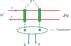
Figure 12: Two pion production from the charmonia transitions in dipole approximation.

The standard approach to ‘the quarkonium – light hadron transitions’ assumes an applicability of the multipole expansion, which means that the quarkonium sizes $r_{c,b}$ are much less than the typical size of the nonperturbative vacuum gluon fluctuation $\lambda_{g}$ (see e.g. [69]). According to this assumption, the dipole approximation can be represented as shown in Fig. 12. However, in ILM $\lambda_{g}\approx\rho$. Using the instanton parameter $\rho=0.33$ fm and the charmonium size $r_{J/\psi}=0.25$ fm (see Table 2) from Eq. (60) we can get the value $g_{J/\psi}=0.28(1-0.2)\simeq 0.22$. From here we can conclude that the correction to the dipole approximation in charmonium case is quite sizable, $\sim 20\%$.

IV Heavy quark correlators with perturbative corrections in ILM

Our previous discussion demonstrated the importance of the nonpertubative contributions for the spectra and wave functions of heavy quarkonia, which might be naturally incorporrated if we will use $Q\bar{Q}$ potential found within ILM approach. We will follow our previous work [77]. In calculations, one should also take into account that the instanton field has a specific $A\sim 1/g$ dependence on the strong coupling $g$. The normalized partition function $Z[j]$ in ILM can be given by an approximate expression

$$Z[j] =\int D\xi Dae^{-[S_{eff}[a,A(\xi)]+(ja)]}\approx\int D\xi e^{-\frac{1}{2}(j_{\mu}S_{\mu\nu}(\xi)j_{\nu})},$$ (61)

which accounts for the perturbative gluons $a_{\mu}$ and their corresponding sources $j_{\mu}$. In derrivation of the partition function in Eq. (61), we neglected the self-interaction terms of order ${\cal O}(a^{3},a^{4})$ , and used the shorthand notations

$$(ja)=\int d^{4}xj_{\mu}^{a}(x)a_{\mu}^{a}(x),\,\,\,j_{\mu}^{a}(x)S_{\mu\nu}^{ab}(x,y,\xi)j_{\nu}^{b}(y).$$

where $S_{\mu\nu}^{ab}(x,y,\xi)$ is a gluon propagator in the presence of the instanton background $A(\xi)$. Since an infinitely heavy quark interacts only through the fourth components of instantons $A_{4}$ and perturbative gluon $a_{4}$ fields, respectively, we need only $S_{44}(\xi)$ components of a gluon propagator.

Now we will focus on analysis of the heavy quark propagator in ILM framework. From Eq. (61) it is seen that the averaged heavy quark propagator ${w}$ with the account of perturbative gluon field fluctuations $a$ is given by the expression

$${w} =\int D\xi Da\exp[-S_{eff}(a,\xi)+(ja)]\left(\theta^{-1}-ga-g\sum_{i}A_{i}\right)^{-1}$$ (62)

$$=\int D\xi\left[\int\left(\theta^{-1}-g\frac{\delta}{\delta j}-g\sum_{i}A_{i}\right)^{-1}\exp\left\{\frac{1}{2}(jS(\xi)j)\right\}\right]_{j=0}.$$ (63)

It is straightforward to prove that

$$\left[\frac{1}{\theta^{-1}-g\frac{\delta}{\delta j}-gA(\xi)}\exp\left(\frac{1}{2}jS(\xi)j\right)\right]_{{}_{j=0}}=\left[\exp\left(\frac{1}{2}\frac{\delta}{\delta a_{a}}S_{ab}(\xi)\frac{\delta}{\delta a_{b}}\right)\frac{1}{\theta^{-1}-ga-gA(\xi)}\right]_{{}_{a=0}}\qquad$$ (64)

Furthermore, this equation can be extended to any correlator. Consequently, the path integral of heavy quark functional $F[A(\xi),a]$ in the approximations discussed above can be given by the equation

$$\int D\xi Da\exp\left\{-S_{eff}[A(\xi),a]\right\}F[A(\xi),a]=\int D\xi\left[\exp\left(\frac{1}{2}\frac{\delta}{\delta a_{a}}S_{ab}(\xi)\frac{\delta}{\delta a_{b}}\right)F[\xi,a]\right]_{a=0}.$$ (65)

Another equation similar to this, in the absence of instanton background $A(\xi)=0$ and for the gluon propagator taken in Coulomb gauge, was suggested before in Ref. [58].

As we mentioned at the subsection I.1, the systematic accounting of the nonperturbative effects in the ILM can be performed in terms of the dimensionless parameter $\kappa$ by using the Pobylitsa equations [59]. The situation here is quite comfortable for the performing systematic analysis of instanton effects, since the $\kappa$ value is very small at the values of instanton parameters discussed above, $\kappa\sim 0.01$.

In order to take into account the perturbative gluons effects, we should perform an expansion in terms of parameter $\alpha_{s}$. As was discussed in the subsection I.1, in ILM on its scale $\bar{\rho}\approx 0.33$ fm we have $\alpha_{s}(\rho)\approx 0.39$. The pure perturbative effects at the leading order appear as linear corrections in $\alpha_{s}$. A systematic analysis, including both the perturbative and nonperturbative effects, requires a double series expansion in terms of $\alpha_{s}$ and $\kappa$. In order to perform such analysis, we may assume that $\alpha_{s}\sim\kappa^{1/2}$, which is quite reasonable according to the phenomenological studies. Consequently, during the calculations one should keep all necessary terms at the order of ${\cal O}(\kappa)$ and ${\cal O}(\alpha_{s}\kappa^{1/2})$.

IV.1 Gluons in ILM

In the above mentioned approximation, the gluon propagator in the instanton medium can be represented by re-scattering series as

$$S(\xi)=S^{0}+\sum_{i}\Delta S^{i}(\xi_{i})+...,\quad\Delta S^{i}(\xi_{i})\equiv S^{i}(\xi_{i})-S^{0},$$

where $S^{0}$ is free gluon propagator, and $S^{i}(\xi_{i})$ is propagator of gluon in the instanton background. The averaged value of gluon propagator $\overline{S}$ in ILM can be found by extending the Pobylitsa’s equation to the gluon case [41]

$$\overline{S}(k)=\frac{1}{k^{2}+M_{g}^{2}(k)}.$$ (66)

Consequently, the perturbative gluons are also acquire the momentum dependent mass, which is defined by the expressions

$$M_{g}(k) =M_{g}(0)F(k),\quad M_{g}(0)=\frac{2\pi}{\rho}\left(\frac{6\kappa}{N_{c}^{2}-1}\right)^{1/2},\quad F(k)=k\rho K_{1}(k\rho).$$ (67)

Here $K_{1}$ is a modified Bessel function of the second type. Using the typical values of instanton parameters $\rho=1/3\,{\rm fm},\,\,R=1\,{\rm fm}$, we can estimate the dynamical gluon mass at zero momentum. Its value is given by $M_{g}(0)\simeq 358\,{\rm MeV}$ and is close to the value of dynamical light quark mass. We can also note, that the dynamical gluon and light quark masses appear at the same order ${\cal O}\big{(}\kappa^{1/2}\rho^{-1}\big{)}$. The gauge invariance of the dynamical gluon mass $M_{g}$ was proven in Ref. [41].

One may wonder if the instantons also generate the nonperturbative gluon-gluon interactions and, in such a way, contribute to the glueballs’ properties. The corresponding investigations in instanton liquid model [60, 61] devoted to the $J^{PC}=0^{++},0^{-+},2^{++}$ glueballs, showed that the instanton-induced forces between gluons lead to the strong attraction in the $0^{++}$ channel, to the strong repulsion in the $0^{-+}$ channel and to the absence of short-distance effects in the $2^{++}$ channel. Consequently, applications of ILM in studies of glueballs predicted hierarchy of the masses $m_{0^{++}}<m_{2^{++}}<m_{0^{-+}}$ and their corresponding sizes $r_{0^{++}}<r_{2^{++}}<r_{0^{-+}}$. These predictions were confirmed by the lattice calculations [62, 63, 64, 65, 66, 67, 68]. For typical values of ILM parameters $\rho=1/3$ fm and $R=1$ fm it has been found [60] that the mass of $0^{++}$ glueball $m_{0^{++}}=1.4\pm 0.2$ GeV and its size $r_{0^{++}}\approx 0.2$ fm, in a nice correspondence with the lattice calculations [62, 63, 64]. Further studies of the $0^{++}$ glueball in ILM [61] gave $m_{0^{++}}=1.29\,-\,1.42$ GeV, which was also in a good agreement with the lattice results [67, 68].

Main conclusion of the studies which we discussed above was that the origin of $0^{++}$ glueball is mostly provided by the short-sized nonperturbative fluctuations (instantons), rather than the confining forces. In a quick summary, we may conclude that ILM provides the promising framework for describing the lowest state glueball’s properties.

IV.2 Heavy quark propagator with perturbative corrections in ILM

Let us now discuss a single heavy quark properties in ILM by estimating the corresponding effects from perturbative and nonperturbative regions, as was done in Ref. [77]. An averaged infinitely heavy quark propagator in ILM according to Eqs.(63)-(64) is given by

$${w}=\!\left.\!\int\!\!D\xi\exp\left[\frac{1}{2}\!\left(\frac{\delta}{\delta a}S(\xi)\frac{\delta}{\delta a}\right)\!\right]\!\frac{1}{\theta^{-1}-ga-gA(\xi)}\right|_{a=0}\!\!\!$$ (68)

where we have used the shorthand notation

$$\left(\frac{\delta}{\delta a}S(\xi)\frac{\delta}{\delta a}\right)=\int d^{4}yd^{4}z\frac{\delta}{\delta a_{a}(y)}S_{ab}(\xi,y,z)\frac{\delta}{\delta a_{b}(z)}.$$ (69)

From our work [77] we can see that in the ILM the heavy quark propagator with perturbative corrections can be written as

$${w}=\int D\xi\left[\theta^{-1}-\sum_{i}\left(gA_{i}(\xi_{i})-g^{2}\left(\Delta S^{i}(\xi_{i})\theta\right)\right)\right]^{-1},$$ (70)

where the last term in the denominator means the heavy quark mass operator, which is formally a correction of the order ${\cal O}(\alpha_{s}\kappa^{1/2})$. Heavy quark propagator Eq. (70) and its special $g\rightarrow 0$ limit expression have similar structures, according to their dependencies on the instanton collective coordinates. We can now extend Pobylitsa’s equation from Ref. [74], which in the approximation of small ${\cal O}(\kappa,\,\alpha_{s}\kappa^{1/2})$ has a form

$${w}^{-1} = \theta^{-1}-\sum_{i}\int\xi_{i}\theta^{-1}\left(\frac{1}{\theta^{-1}-gA_{i}(\xi_{i})}-\theta\right)\theta^{-1}-g^{2}\left((\bar{S}-S^{0})\theta\right).$$

In the last term the averaged gluon propagator $\bar{S}$ is given by Eq. (66). In such a way, the second term in the right side of Eq. (41) leads to the ILM heavy quark mass shift $\Delta M_{Q}^{{\rm dir}}$ with the corresponding order ${\cal O}(\kappa),$ while the third term is ILM-modified perturbative gluon contribution to the heavy quark mass $\Delta M_{Q}^{{\rm pert}}$, which is formally of order ${\cal O}(\alpha_{s}\kappa^{1/2})$, respectively. We note that the direct mass contribution to the quark mass in instanton background $\Delta M_{Q}^{{\rm pert}}$ was calculated first in Ref. [74]. Numerically, we can estimate that in ILM

$$-\Delta M_{Q}^{{\rm pert}}\sim\frac{2}{N_{c}}\,\alpha_{s}M_{g}(0)\sim\Delta M_{Q}^{{\rm dir}}\simeq 70\,{\rm MeV}.$$ (71)

We see that ILM perturbative $\Delta M_{Q}^{{\rm pert}}$ and ILM direct $\Delta M_{Q}^{{\rm dir}}$ corrections to the heavy quark mass almost completely cancel each other. This estimate is in agreement with the above made assumptions ${\cal O}(\alpha_{s}\kappa^{1/2})\sim{\cal O}(\kappa)$.

IV.3 Heavy quarks singlet potential with perturbative corrections in ILM

Heavy quarks $Q\bar{Q}$ correlator in ILM can be calculated from the operator

$${W}=\int D\xi\exp\left[\frac{1}{2}\sum_{i,j=1}^{2}\left(\frac{\delta}{\delta a_{a}^{(i)}}S_{ab}^{(ij)}(\xi)\frac{\delta}{\delta a_{b}^{(j)}}\right)\right]\left.\frac{1}{D^{(1)}-ga^{(1)}}\frac{1}{\bar{D}^{(2)}-g\bar{a}^{(2)}}\right|_{a=0},$$ (72)

where the operator $D^{(1)}$ is defined as $D^{(1)}=\theta^{-1}-gA^{(1)}(\xi)$ and, $a^{(1)}$ and $A^{(1)}$ are the corresponding fields projections to the line $L_{1}$, respectively. Similarly, one has $\bar{D}^{(2)}=\theta^{-1}-g\bar{A}^{(2)}(\xi)$ where $\bar{a}^{(2)}$ and $\bar{A}^{(2)}$ are the corresponding fields projections to the line $L_{2}$, respectively (see Fig. 9). Consequently, extended Pobylitsa’s equation in the approximation ${\cal O}(\kappa,\alpha_{s}\kappa^{1/2})$ has the solution [77]:

$${W}^{-1}={w}^{(1)-1}{\bar{w}}^{(2)-1}-\sum_{i}\int d\xi_{i}\theta^{(1)-1}$$ (73)

$$\times\left(\frac{1}{D_{i}^{(1)}}-\theta^{(1)}\right)\theta^{(1)-1}\theta^{(2)-1}\left(\frac{1}{\bar{D}_{i}^{(2)}}-\theta^{(2)}\right)\theta^{(2)-1}-g^{2}\frac{\lambda_{a}}{2}\frac{\bar{\lambda}_{b}}{2}\int D\xi\,S_{ab}^{(12)},$$ (74)

where ${w}^{(1)-1}$ is given by Eq.(41). Note, that the equation for ${\bar{w}}^{(2)-1}$ also can be written in a form similar to Eq.(41).

It is clear that ILM contributions to the heavy quark masses $\Delta M_{Q}^{{\rm dir}}$ and $\Delta M_{Q}^{{\rm pert}}$ are coming from the first term of the Eq. (74), while $V_{{\rm dir}}(r)$ - from second, and $V_{{\rm pert}}(r)$ - from third one. First we note that

$$V_{{\rm pert}}(r)=V_{C}(r)+\Delta V_{{\rm pert}}(r),\,\,V_{C}(r)=-\frac{16\pi\alpha_{s}}{3}\int\frac{d^{3}q}{(2\pi)^{3}}e^{i\vec{q}\vec{r}}\frac{1}{q^{2}},\,\,\,$$

$$\Delta V_{{\rm pert}}(r)=\frac{16\pi\alpha_{s}}{3}\int\frac{d^{3}q}{(2\pi)^{3}}e^{i\vec{q}\vec{r}}\frac{M^{2}(q)}{q^{2}(q^{2}+M_{g}^{2}(q))},\,\,\,q=|\vec{q}|,$$ (75)

where $M_{g}(q)$ is given by Eq. (67), $V_{C}(r)$ is the perturbative QCD one gluon exchange (OGE) potential and $\Delta V_{{\rm pert}}(r)$ is ILM contribution $\sim O(\kappa^{1/2}\alpha_{s})$, which is positively defined. We can find now from the Eq. (74) the ILM contribution to the total energy of $Q\bar{Q}$ system in singlet color state as

$$\Delta E_{{\rm ILM}}(r)=\Delta E_{{\rm ILM}}^{{\rm dir}}(r)+\Delta E_{{\rm ILM}}^{{\rm pert}}(r),\,\,\,\Delta E_{{\rm ILM}}^{{\rm dir}}(r)=2\Delta M_{Q}^{{\rm dir}}+V_{{\rm dir}}(r),\,\,\,\Delta E_{{\rm ILM}}^{{\rm pert}}(r)=2\Delta M_{Q}^{{\rm pert}}+\Delta V_{{\rm pert}}(r)$$ (76)

The direct instanton contribution $\Delta E^{{\rm dir}}(r)$ was calculated early in Ref. [74]. It is clear that $\Delta E^{{\rm dir}}(r)$ is positively defined, since $\Delta E^{{\rm dir}}(0)=0$ and $\Delta E^{{\rm dir}}(\infty)=2\Delta M_{Q}^{{\rm dir}}>0$. On the other hand, comparing Eqs. (71) and (75), we find that $\Delta E_{{\rm ILM}}^{{\rm pert}}(r)$ is negatively defined, since $\Delta E_{{\rm ILM}}^{{\rm pert}}(0)=0$ and $\Delta E_{{\rm ILM}}^{{\rm pert}}(\infty)=2\Delta M_{Q}^{{\rm pert}}<0$. So, the two contributions almost cancel each other, and the total ILM contribution $\Delta E_{{\rm ILM}}(r)$ becomes small, as could be seen from the Fig. 13. For this reason we expect small influence of the instantons on the heavy quarkonia spectra and wave functions.

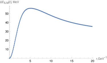
Figure 13: ILM total contribution $\Delta E_{{\rm ILM}}(r)$ to the energy of singlet $Q\bar{Q}$ system as a function of their relative distance. Basic parameters are taken as: $R=1$ fm, $\rho=0.33$ fm, $\alpha_{s}(\rho)=0.39$.

The relative sizes of all possible instanton effects in comparison with the results corresponding to the Cornell’s model results [72] found to be few percents in the ILM [75].

V Summary

QCD vacuum instantons generate the nonperturbative interactions among gluons, light and heavy quarks. The phase state of the instanton ensemble in the framework of the Instanton Liquid Model (ILM) is controlled by the packing parameter $\kappa=\rho^{4}/R^{4}$, which quantifies the fraction of the space occupied by instantons. Detailed considerations of the instanton size $\rho$ and inter-instanton distance $R$ showed that in average $\bar{\rho}\approx 1/3$ fm, and $R\approx 1$ fm, so the packing parameter is comfortably small $\kappa\approx 0.01$. This finding can be used as expansion parameter within Pobylitsa equations for averaging over the instanton collective coordinates in various correlators. Most essential conclusions can be made by considering the strength of particle-instanton interaction. We found that the dominance of zero-modes in light quark determinant provides strong light quark-instanton interaction, which leads to dynamical light quark mass $M_{q}\approx 360$ MeV$\sim\kappa^{1/2}\rho^{-1}$. In contrast, for heavy quarks their interaction with gluons is controlled mainly by their mass, and for this reason they rather weakly interact with instantons, so the instanton contribution to their mass is small and given by $\Delta M_{Q}^{{\rm dir}}\approx 70$ MeV$\sim\kappa\rho^{-1}.$ It is clear that instantons generate nonperturbative interactions between particles, which cross simultaneously the same instanton. This mechanism perfectly describes spontaneous breaking of chiral symmetry (SBChS), which is most essential phenomena for light quarks physics. On the other hand, this nonperturbative mechanism also contributes to the interaction between light and heavy quarks and might be used for studies of nonperturbative effects in light-heavy quarks systems. The manuscript provides the framework for the calculations of various problems for such a systems. As an example, we considered in detail the process of pion pair emission in decays of excited heavy quarkonia. This analysis requires calculation of heavy quarkonia spectra and their wave functions. While usually this analysis is done using perturbative QCD, which describes them fairly well, in our study we calculated ILM corrections to these quantities. In the calculations we took into account the perturbative gluon properties in the instanton medium. We found that perturbative gluon-instanton interaction is strong, as happens for light quarks, and the instanton-generated dynamical gluon mass $M_{g}\approx 360$ MeV$\sim\kappa^{1/2}\rho^{-1}$ is comparable to that of the light quarks. Finally, we found that $O(\kappa)$ contributions to the singlet heavy $Q\bar{Q}$ system energy almost completely cancel similar $O(\alpha_{s}\kappa^{1/2})$ contributions, and thus nonperturbative interactions have small influence on the heavy quarkonia spectrum and wave functions. In our evaluation we neglect possible contributions of the higher Fock state $Q\bar{q}q\bar{Q}$, which might be relevant at large scale distances $\sim 1/M_{q}\sim 0.5$ fm. We are planning to calculate this and similar problems related to the heavy-light quarks systems within ILM.

References

- [1] T. Schafer and E. V. Shuryak, Rev. Mod. Phys. 70 (1998) 32.
- [2] E. Shuryak, Lectures on nonperturbative QCD [arXiv:hep-ph/1812.01509 [hep-ph]].
- [3] D. Diakonov, Prog. Part. Nucl. Phys. 51 (2003) 173.
- [4] E. V. Shuryak, Nucl. Phys. B 203 (1982), 93.
- [5] D. Diakonov and V. Y. Petrov, Nucl. Phys. B 245 (1984), 259-292
- [6] L. D. Faddeev, Looking for multi-dimensional solitons in: Non-local Field Theories (Dubna, 1976).
- [7] R. Jackiw and C. Rebbi, Phys. Rev. Lett. 37 (1976) 172.
- [8] A. Belavin, A. M. Polyakov, A. Schwartz and Y, Tyupkin Phys. Lett. B 59 (1975) 85.
- [9] A. M. Shifman, A. I. Vainshtein and V. I. Zakharov, Nucl. Phys. B 147 (1979) 385.
- [10] G. ’t Hooft, Phys. Rev. D 14 (1976), 3432-3450 [erratum: Phys. Rev. D 18 (1978), 2199]
- [11] C. G. Callan, Jr., R. F. Dashen and D. J. Gross, Phys. Rev. D 17 (1978), 2717
- [12] M. Chu, J. Grandy, S. Huang and J. W. Negele, Phys. Rev. D 49 (1994) 6039.
- [13] J. W. Negele, Nucl. Phys. B Proc. Suppl. 73 (1999) 92.
- [14] T. A. DeGrand, Phys. Rev. D 64 (2001) 094508.
- [15] P. Faccioli and T. A. DeGrand, Phys. Rev. Lett. 91 (2003) 182001.
- [16] R. Millo and P. Faccioli, Phys. Rev. D 84 (2011) 034504.
- [17] H. Leutwyler, Czech. J. Phys. 52 (2002), B9-B27 [arXiv:hep-ph/0212325 [hep-ph]].
- [18] C. k. Lee and W. A. Bardeen, Nucl. Phys. B 153 (1979), 210-236
- [19] D. Diakonov and V. Y. Petrov, Nucl. Phys. B 272 (1986), 457-489
- [20] D. Diakonov, V. Polyakov and C. Weiss, Nucl. Phys. B 461 (1996) 539.
- [21] T. C. Kraan and P. van Baal, Phys. Lett. B 428 (1998) 268.
- [22] T. C. Kraan and P. van Baal, Nucl. Phys. B 533 (1998) 627.
- [23] K. M. Lee and C. H. Lu, Phys. Rev. D 58 (1998) 025011.
- [24] D. Diakonov, Nucl. Phys. B Proc. Suppl. 195 (2009) 5.
- [25] Y. Liu, E. Shuryak and I. Zahed, Phys. Rev. D 92 (2015) 085006.
- [26] E. Shuryak and I. Zahed, Phys. Rev. D 92 (2015) 085007.
- [27] M. Musakhanov and F. C. Khanna, Phys. Lett. B 395 (1997) 298.
- [28] E. D. Salvo and M. Musakhanov, Eur. Phys. J. C 5 (1998) 501.
- [29] M. Musakhanov, Eur. Phys. J. C 9 (1999) 235.
- [30] M. Musakhanov, Nucl. Phys. A 699 (2002) 340.
- [31] M. Musakhanov and H. C. Kim, Phys. Lett. B 572 (2003) 181.
- [32] H. C. Kim, M. Musakhanov and M. Siddikov, Phys. Lett. B 608 (2005) 95.
- [33] H. C. Kim, M. M. Musakhanov and M. Siddikov, Phys. Lett. B 633 (2006), 701-709 [arXiv:hep-ph/0508211 [hep-ph]].
- [34] K. Goeke, M. Musakhanov and M. Siddikov, Phys. Rev. D 76 (2007) 076007.
- [35] K. Goeke, H. C. Kim, M. Musakhanov and M. Siddikov, Phys. Rev. D 76 (2007) 116007.
- [36] K. Goeke, M. Musakhanov and M. Siddikov, Phys. Rev. D 81 (2010) 054029.
- [37] M. Musakhanov, PoS Baldin-ISHEPP-XXI (2012) 008.
- [38] M. Musakhanov, PoS Baldin-ISHEPPXXII (2015) 012.
- [39] M. Musakhanov, EPJ Web Conf. 182 (2018) 02092.
- [40] M. Musakhanov, EPJ Web Conf. 182 (2018) 02092.
- [41] M. Musakhanov and O. Egamberdiev, Phys. Lett. B 779 (2018) 206.
- [42] S. R. Coleman and E. Weinberg, Phys. Rev. D 7(1973) 1888.
- [43] R. Jackiw, Phys. Rev. D 9(1974) 1686.
-
[44]
P. O. Bowman, private communication ()-dependence.
See also P. O. Bowman, U. M. Heller, D. B. Leinweber, M. B. Parappilly, A. G. Williams and J. b. Zhang,
Phys. Rev. D 71 (2005) 054507 [arXiv:hep-lat/0501019]. - [45] J. Gasser and H. Leutwyler, Annals Phys. 158 (1984) 142.
- [46] H. Leutwyler, arXiv:hep-ph/0612112.
- [47] H. Leutwyler, arXiv:0706.3138 [hep-ph].
- [48] C. Aubin et al. [MILC Collaboration], Phys. Rev. D 70 (2004) 114501 [arXiv:hep-lat/0407028].
- [49] L. Del Debbio, L. Giusti, M. Luscher, R. Petronzio and N. Tantalo, JHEP 0702 (2007) 056 [arXiv:hep-lat/0610059].
- [50] G. Colangelo, J. Gasser and H. Leutwyler, Nucl. Phys. B 603 (2001) 125 [arXiv:hep-ph/0103088].
- [51] C. Bernard et al., arXiv:hep-lat/0611024.
- [52] Ph. Boucaud et al. [ETM Collaboration], arXiv:hep-lat/0701012.
- [53] S. Digal, O. Kaczmarek, F. Karsch and H. Satz, Eur. Phys. J. C 43 (2005) 71.
- [54] E. Eichten, K. Gottfried, T. Kinoshita, K. Lane and T. M. Yan, Phys. Rev. D 21 (1980) 203.
- [55] Y. He, F. Wang and C. W. Wong, Phys. Lett. B 168 (1986) 177.
- [56] W. Weise, Quarks, chiral symmetry and dynamics of nuclear constituents in: Quarks and Nuclei, (World Scientific,1985) p. 57-188.
- [57] R. Tegen, Nucleon form factors from elastic scattering of polarized leptons (, , ) from polarized nucleons in:Weak and Electromagnetic Interactions in Nuclei (Springer, 1986) p.435.
- [58] L. S. Brown and W. I. Weisberger, Phys. Rev. D 20 (1979) 3239.
- [59] P. Pobylitsa Phys. Lett. B 226 (1989) 387.
- [60] T. Schafer and E. V. Shuryak, Phys. Rev. Lett. 75 (1995) 1707.
- [61] M. C. Tichy and P. Faccioli, Eur. Phys. J. C 63 (2009) 423.
- [62] P. de Forcrand and K. F. Liu, Phys. Rev. Lett. 69 (1992) 245.
- [63] D. Weingarten, Nucl. Phys. B Proc. Suppl. 34 (1994) 29.
- [64] H. Chen, J. Sexton, A. Vaccarino and D. Weingarten, Nucl. Phys. B Proc. Suppl. 34 (1994) 357.
- [65] C. J. Morningstar and M. J. Peardon, Phys. Rev. D 60 (1999) 034509.
- [66] A. Athenodorou and M. Teper, The glueball spectrum of SU(3) gauge theory in 3+1 dimension’ [arXiv: hep-lat/2007.06422].
- [67] H. B. Meyer and M. J. Teper, Phys. Lett. B 605 (2005) 344.
- [68] H. B. Meyer, Glueball regge trajectories [arXiv: hep-lat/0508002].
- [69] M. B. Voloshin, Prog. Part. Nucl. Phys. 61 (2008) 455.
- [70] G. S. Bali, Phys. Rept. 343 (2001) 1. [hep-ph/0001312].
- [71] N. Brambilla, Y. Sumino and A. Vairo, Phys. Lett. B 513 (2001), 381-390 [arXiv:hep-ph/0101305 [hep-ph]].
- [72] V. Mateu, P. G. Ortega, D. R. Entem and F. Fernández, Eur. Phys. J. C 79 (2019) 323. [arXiv:1811.01982 [hep-ph]].
- [73] T. Mannel, R. Urech, Z Phys C 73 (1997) 541.
- [74] D. Diakonov, V. Y. Petrov and P. V. Pobylitsa, Phys. Lett. B 226 (1989) 372.
- [75] U. T. Yakhshiev, H. .C. Kim, M. Musakhanov, E. Hiyama and B. Turimov, Chin. Phys. C 41 (2017) 083102.
- [76] U. T. Yakhshiev, H. C. Kim and E. Hiyama, Phys. Rev. D 98 (2018) 114036.
- [77] M. Musakhanov, N. Rakhimov and U. T. Yakhshiev, Phys. Rev. D 102 (2020) 076022.