Reoriented Memory of Galaxy Spins for the Early Universe

Abstract

Galaxy spins are believed to retain the initially acquired tendency of being aligned with the intermediate principal axes of the linear tidal field, which disseminates a prospect of using them as a probe of early universe physics. This roseate prospect, however, is contingent upon the key assumption that the observable stellar spins of the present galaxies measured at inner radii have the same alignment tendency toward the initial tidal field as their dark matter counterparts measured at virial limits. We test this assumption directly against a high-resolution hydrodynamical simulation by tracing back the galaxy component particles back to the protogalactic stage. It is discovered that the galaxy stellar spins at $z=0$ have strong but reoriented memory for the early universe, exhibiting a significant signal of cross-correlation with the major principal axes of the initial tidal field at $z=127$. An analytic single-parameter model for this reorientation of the present galaxy stellar spins relative to the initial tidal field is devised and shown to be in good accord with the numerical results.

1 Introduction

The directions of galaxy angular momentum vectors, which will be referred to as the galaxy spins throughout this paper, have been regarded as one of those very few near-field observables that are analytically tractable within the linear perturbation theory (White, 1984; Catelan & Theuns, 1996), which generically predicts preferential alignments of the proto-galaxy spins with the intermediate principal axes of the initial tidal field (Lee & Pen, 2000, 2001; Porciani et al., 2002a, b). This version of the linear perturbation theory adapted for the origin of the galaxy angular momentum is often dubbed the linear tidal torque theory (LTTT). The initially acquired alignment tendency predicted by the LTTT is believed to be well retained during the subsequent nonlinear evolution (e.g., Lee & Erdogdu, 2007; Zhang et al., 2015; Lee et al., 2018; Motloch et al., 2021), even though the galaxy spins swing and flip with respect to the cosmic web through hierarchical merging process (e.g., Aragón-Calvo et al., 2007; Hahn et al., 2007; Paz et al., 2008; Codis et al., 2012; Trowland et al., 2013; Libeskind et al., 2013; Dubois et al., 2014; Codis et al., 2015; Wang & Kang, 2017; Codis et al., 2018; Ganeshaiah Veena et al., 2018; Wang et al., 2018; Kraljic et al., 2020; Lee et el., 2020; Lee & Libeskind, 2020).

Several $N$-body simulations have indeed confirmed the existence of the alignments between the spins of galactic halos and the intermediate principal axes of the local tidal field even in the nonlinear regime ($z\leq 2$), although the alignment tendency gradually becomes weaker at lower redshifts and on the lower mass scales (e.g., Forero-Romero et al., 2014; Chen et al., 2016; Lee et el., 2020; Lee et al., 2021). These numerical evidences inspired several authors to investigate a possibility of probing the physics of early universe with the galaxy spins. For instance, Yu et al. (2020) showed that the degree of chiral asymmetry could in principle be constrained by measuring the present galaxy spins. Motloch et al. (2021) suggested that the galaxy spins be a useful diagnostics of cosmic inflation and primordial gravitational waves. Lee & Libeskind (2020) found that the threshold mass at which the alignments between the galaxy spins and local tidal field become negligibly weak has a potential to distinguish between viable dark energy candidates. The success of this new probe, however, depends entirely on how strongly the present galaxy stellar spins are cross-correlated with the initial tidal field, which is not necessarily guaranteed by their correlations with the local tidal fields, i.e., surrounding cosmic web.

Motloch et al. (2021) reported a $2.7\sigma$ signal of the alignments between the present galaxy stellar spins and reconstructed initial galaxy dark matter (DM) spins from the observational data. The former was determined from the Sloan Digital Sky Survey (SDSS) galaxies whose morphologies had been classified by the Galaxy Zoo project (Lintott et al., 2008), while the latter was evaluated according to the LTTT with the initial density and tidal fields reconstructed by the ELUCID algorithm (Wang et al., 2016). Although this observational signal supports the conservation of the galaxy spins, it still cannot be directly translated into the existence of the alignments between the present galaxy stellar spins and the intermediate principal directions of the initial tidal field.

Furthermore, a recent numerical experiment based on a high-resolution hydrodynamical simulation found that the galaxy spins exhibit a radius dependent transition with respect to the local tidal field (Moon & Lee, 2023). Unlike the galaxy virial spins measured at the virial radii, $r_{\rm v}$, the galaxy inner spins measured at inner radii $r<r_{\rm v}$ were found to be aligned with the major principal axes of the local tidal field, depending on the scale. In true observations, the galaxy stellar spins can be measured only at $r\lesssim 2R_{1/2\star}$ (e.g., Romanowsky et al., 2003; Coccato et al., 2009) with the stellar half-mass radius $R_{1/2\star}$, much more inner regions than the virial limits. Meanwhile, what is predicted to be aligned with the intermediate principal directions of the initial tidal field is the galaxy virial spins (Lee & Pen, 2000, 2001).

The detection of the radius dependent spin transition phenomena gives a warning to any parallel comparison between the observable galaxy stellar spins and the predictions of LTTT. It is an essential prerequisite to explore if and how the observable stellar spins of the present galaxies measured at $\lesssim 2R_{1/2\star}$ are truly aligned with the principal axes of the initial tidal field smoothed on the galactic scale $\sim 0.5\,h^{-1}{\rm Mpc}$ (Bardeen et al., 1986), before using the galaxy spins as a new window on the early universe. In this Paper, we set out to fulfill this core mission.

2 Alignments between Present Galaxy Spins and Initial Tidal Fields

2.1 Numerical Analysis

We make use of the subhalos resolved via the SUBFIND algorithm (Springel et al., 2001) in the TNG300-1 hydrodynamical simulation of the IllustrisTNG project (Marinacci et al., 2018; Naiman et al., 2018; Nelson et al., 2018; Pillepich et al., 2018; Springel et al., 2018; Nelson et al., 2019), referring to them as the galaxies. The simulation was performed on a periodic cubic box of a side length $205\,h^{-1}{\rm Mpc}$ with a total of $2\times 2500^{3}$ elements for the Planck $\Lambda{\rm CDM}$ (cosmological constant $\Lambda$+cold dark matter) universe (Planck Collaboration et al., 2016). A half of the elements behaves as collisionless DM particles that only gravitationally interact, while the other half is the collisional baryons that can cool down to form stars. The average mass resolutions of the DM and baryonic elements attain $5.9\times 10^{7}\,M_{\odot}$ and $1.1\times 10^{7}\,M_{\odot}$, respectively. See the IllustrisTNG webpage for a full information on the codes and hydrodynamical physics implemented into the simulation.

Applying the cloud-in-cell method to the spatial distributions of all DM and baryon elements at $z=127$ where the simulation starts, we first construct a real-space initial density field, $\delta({\bf q})$, on the $512^{3}$ grids and then Fourier-transform it into $\delta({\bf k})$, with wave vector ${\bf k}=k(\hat{k}_{l})$. The initial tidal field, ${\bf T}\equiv(T_{ln})$, convolved with a Gaussian kernel of scale radius $R_{f}$, is then determined via an inverse Fourier transformation of $\hat{k}_{l}\hat{k}_{n}\exp(-k^{2}R^{2}_{f}/2)\delta({\bf k})$ as in Moon & Lee (2023). Throughout this paper, we will consider two different kernel scales, $R_{f}/(\,h^{-1}{\rm Mpc})=0.5$ and $1$.

For the current analysis, a total of $44956$ galaxies are selected at $z=0$, which have total masses $M_{g}$ in a range of $11.8\leq\log\tilde{M}_{g}\leq 12.6$ with $\tilde{M}_{g}\equiv M_{g}/(\,h^{-1}\,M_{\odot})$ and contain $300$ or more stellar particles ($n_{s}\geq 300$) within $2R_{1/2\star}$ (Bett et al., 2007). The present stellar spin of each selected galaxy is determined as $\hat{\bf j}_{\star}\equiv{\bf J}_{\star}(z=0)/|{\bf J}_{\star}(z=0)|$ with ${\bf J}_{\star}(z=0)\equiv\sum_{\gamma=1}^{n_{s}}{m_{\star\gamma}}\,({\bf x}_{c}-{\bf x}_{\gamma})\times({\bf v}_{c}-{\bf v}_{\gamma})$, where $m_{\star\gamma}$, ${\bf x}_{\gamma}$ and ${\bf v}_{\gamma}$ denote the mass, comoving position and peculiar velocity of the $\gamma$th stellar particle, respectively, while ${\bf x}_{c}$ and ${\bf v}_{c}$ are the comoving position and peculiar velocity of the potential minimum (coinciding well with the galaxy center of mass), respectively.

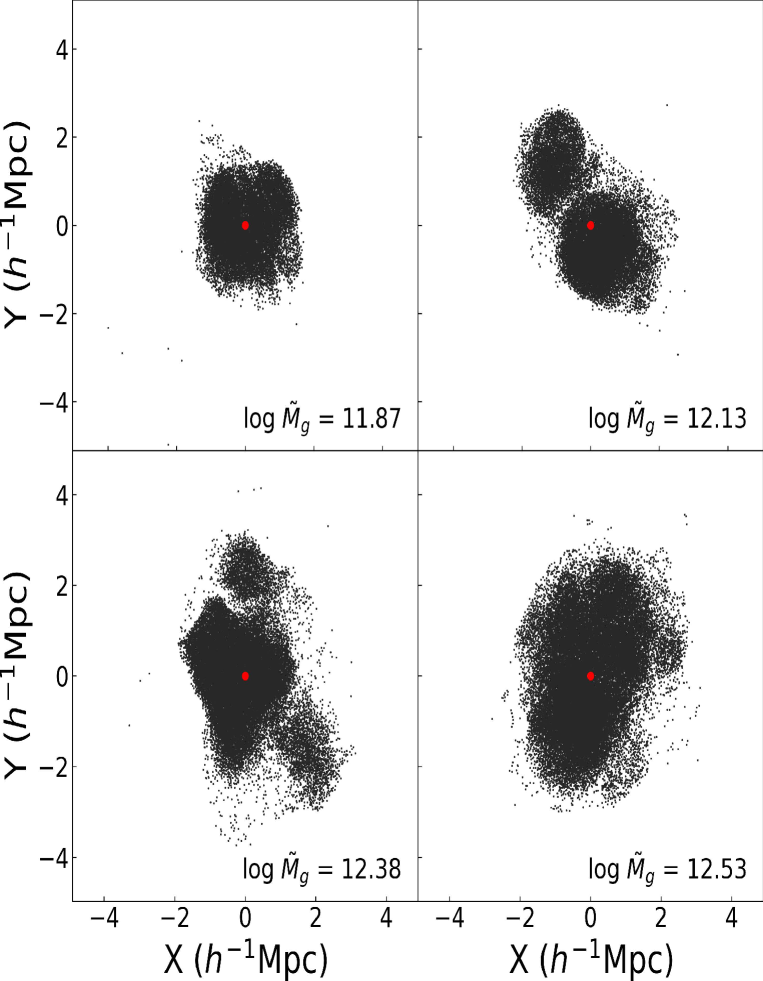
Figure 1: Two dimensional projected images of randomly selected four proto-galaxies in the $\hat{\bf x}$-$\hat{\bf y}$ plane at $z=127$.

Tracing all constituent DM particles of each selected galaxy enclosed within $r_{\rm v}$ back to $z=127$, we find its proto-galactic sites and locate its initial center of mass, ${\bf q}_{c}$. Figure 1 shows the two dimensional projected images of randomly selected proto-galaxies with their center of masses marked by red dots in four different mass sections. As can be seen, the spatial extents of the lowest-mass proto-galaxies are larger than the smoothing scales, $R_{f}/(\,h^{-1}{\rm Mpc})\leq 1$, which is important to ascertain since the initial tidal field smoothed on the scales larger than the spatial extents of the proto-galactic sites could produce overdamped alignment signals. The initial tidal field, ${\bf T}({\bf q}_{c})$, is put through a similarity transformation to yield its three orthonormal eigenvectors, $\{\hat{\bf t}_{1}({\bf q}_{c}),\hat{\bf t}_{2}({\bf q}_{c}),\hat{\bf t}_{3}({\bf q}_{c})\}$, parallel to its major, intermediate and minor principal axes, respectively. The alignments of the present galaxy stellar spins and the principal axes of the initial tidal field as a function of $\log\tilde{M}_{g}$ are then evaluated as $\{\langle|\hat{\bf j}_{\star}\cdot\hat{\bf t}_{l}|\rangle\}_{l=1}^{3}$, where the ensemble averages are taken over the galaxies whose masses fall in a given differential interval of $[\log\tilde{M}_{g},\log\tilde{M}_{g}+d\log\tilde{M}_{g}]$.

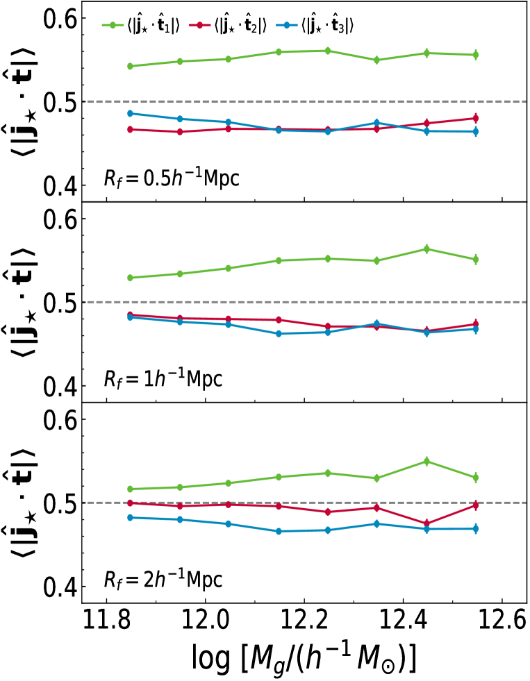
Figure 2: Alignments of the present galaxy stellar spins at $z=0$ and three principal axes of the initial tidal field at $z=127$ as a function of the logarithms of the total galaxy mass for three different cases of the smoothing scale. In line with observations, the present galaxy stellar spins are measured at $2R_{1/2\star}$.

In Figure 2 we show $\{\langle|\hat{\bf j}_{\star}\cdot\hat{\bf t}_{1}|\rangle$ (green line), $\langle|\hat{\bf j}_{\star}\cdot\hat{\bf t}_{2}|\rangle$ (red line), $\langle|\hat{\bf j}_{\star}\cdot\hat{\bf t}_{3}|\rangle\}$ (blue line) versus $\log\tilde{M}_{g}$ for three different cases of $R_{f}/(\,h^{-1}{\rm Mpc})=0.5$, $1$ and $2$ in the top, middle and bottom panels, respectively. The associated errors are computed as one standard deviation in the ensemble averages. As can be seen, the present galaxy stellar spins are preferentially aligned with the major (rather than intermediate) principal axes with the initial tidal field for all of the three cases of $R_{f}$, unlike the expectation based on the LTTT and angular momentum conservation (Lee & Pen, 2000, 2001). Note that the $\hat{\bf j}_{\star}$–$\hat{\bf t}_{1}$ alignment mildly dwindles as $\log\tilde{M}_{g}$ decreases and as $R_{f}$ increases.

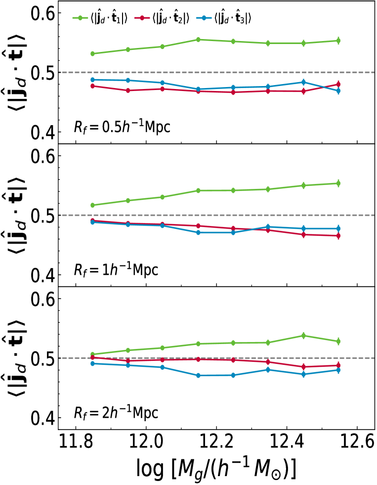
Figure 3: Same as Figure 2 but with the present galaxy DM inner spins measured at $2R_{1/2\star}$.

To see whether or not this somewhat unexpected $\hat{\bf j}_{\star}$–$\hat{\bf t}_{1}$ alignment is caused by some baryonic effects in the subsequent evolution, we measure the present galaxy DM spins, $\hat{\bf j}_{d}$, from the DM particles enclosed within $2R_{1/2\star}$ and repeat the same analysis, the results of which are shown in Figure 3. As can be seen, little difference exists between $\hat{\bf j}_{d}$ and $\hat{\bf j}_{\star}$ in the tendencies and strengths of their alignments with $\{\hat{\bf t}_{l}({\bf q}_{c})\}_{l=1}^{3}$, which clearly rules out any baryon effects as a possible origin of the $\hat{\bf j}_{\star}$–$\hat{\bf t}_{1}$ alignment.

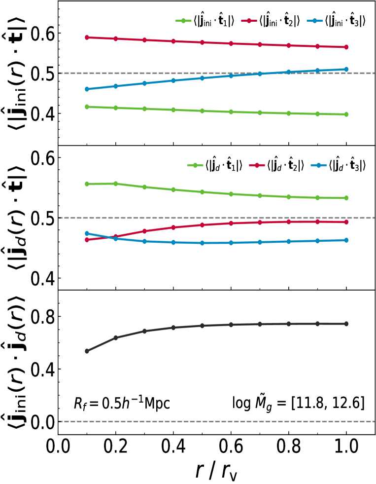
Figure 4: (Top panel): alignments between the initial galaxy spins measured at inner radii $r\leq r_{\rm v}$ and three principal axes of the initial tidal field at the same epoch as a function of the inner to virial radius ratio for the case of $R_{f}=0.5/(\,h^{-1}{\rm Mpc})$. (Middle panel): same as the top panel but with the present galaxy spins at $z=0$. (Bottom panel): alignments between the initial and present galaxy spins.

To test the LTTT whose archetypal prediction was the alignments between the initial galaxy spins and the intermediate principal axes of the initial tidal field, we measure the initial galaxy DM spins, $\hat{\bf j}_{\rm ini}\equiv\hat{\bf j}(z=127)$, from the initial positions and peculiar velocities of the DM particles that end up being within $r\leq r_{\rm v}$ from the present galaxy centers at $z=0$, and investigate their alignments with the principal axes of the initial tidal field, $\{\langle|\hat{\bf j}_{\rm ini}\cdot\hat{\bf t}_{l}|\rangle\}_{l=1}^{3}$, as a function of $r/r_{\rm v}$. The top panel of Figure 4 plots $\{\langle|\hat{\bf j}_{\rm ini}(r)\cdot\hat{\bf t}_{l}|\rangle\}_{l=1}^{3}$ versus $r/r_{\rm v}$ for the case of $R_{f}/(\,h^{-1}{\rm Mpc})=0.5$, demonstrating that the initial galaxy spins are indeed well aligned with the intermediate principal axes of the initial tidal field in the whole range of $0\leq r/r_{\rm v}\leq 1$. This result confirms that the LTTT predictions hold true not only for the virial spins but also for the inner spins as far as they are measured at the initial epochs. For comparison, the radius dependence of the alignment tendency of the present galaxy DM spins, $\hat{\bf j}_{d}(r)$, with the initial tidal field is also investigated and shown in the middle panel of Figure 4. Note that $\hat{\bf j}_{d}(r)$ are always aligned with $\hat{\bf t}_{1}$ not only for the case of $r<r_{\rm v}$ but also for the case $r=r_{\rm v}$.

Questioning if this obvious difference between the present and initial galaxy spins in their alignment tendencies toward the initial tidal field indicates a complete breakdown of angular momentum conservation, we also compute the alignments between the present and initial galaxy DM spins, $\langle\hat{\bf j}_{d}(z)\cdot\hat{\bf j}_{\rm ini}(r)\rangle$ as a function of $r/r_{\rm v}$, which are shown in the bottom panel of Figure 4. As can be seen, the present galaxy spins are indeed strongly aligned with the initial galaxy spins, confirming that the galaxy angular momentum are quite well conserved even during the nonlinear evolution.

A central implication of the results shown in Figs. 2–4 is the following. Despite that the LTTT is indeed quite successful in describing the correlations between the galaxy spins and the tidal field measured at the same initial epochs and that the present galaxy spins are well aligned with the initial counterparts, the validity of the LTTT cannot be extrapolated to predict the cross-correlations between the present galaxy inner spins (or stellar spins) and the initial tidal field since the present galaxy inner spins are reoriented from their initial versions. The more inner radii the present spins are measured at, the more strongly their alignment tendency deviates from the prediction of the LTTT.

2.2 Analytical Modeling

For a better understanding of the numerical results presented in Section 2.1, we construct an analytic model for the probability density function, $p(|\hat{\bf j}_{\star}\cdot\hat{\bf t}_{1}|)$. As in Lee & Pen (2001), we assume that the conditional joint probability density function of three coordinates of the angular momentum vectors of the galaxy stellar components given a tidal field, $p(J_{\star 1},J_{\star 2},J_{\star 3}|\tilde{\bf T})$, can be well approximated by the following multivariate Gaussian distribution (see also Lee, 2019)

$$p(J_{\star 1},\ J_{\star 2},\ J_{\star 3}|\tilde{\bf T})=\frac{1}{\sqrt{(2\pi)^{3}{\rm det}({\bf\Sigma})}}\exp\left[-\frac{1}{2}\left({\bf J}^{t}_{\star}\cdot{\bf\Sigma}^{-1}\cdot{\bf J}_{\star}\right)\right]\,,$$ (1)

where $\tilde{\bf T}$ is the traceless version of ${\bf T}$, and ${\bf\Sigma}=({\Sigma}_{ln})$ is the covariance matrix whose components are given as ${\Sigma}_{ln}\equiv\langle{J}_{\star l}{J}_{\star n}|\tilde{\bf T}\rangle$.

Marginalize $p(J_{\star 1},J_{\star 2},J_{\star 3}|\tilde{\bf T})$ over the magnitude of ${\bf J}_{\star}$, we compute the conditional probability density function of the galaxy stellar spins as

$$p(\hat{j}_{\star 1},\ \hat{j}_{\star 2},\ \hat{j}_{\star 3}|\hat{\bf T}) = \int\,p({\bf J}_{\star}|\tilde{\bf T})J^{2}_{\star}\,dJ_{\star}$$ (2)

$$= \frac{1}{4\pi\left[{\rm det}(\hat{\bf\Sigma})\right]^{1/2}}\left(\hat{\bf j}_{\star}\cdot\hat{\bf\Sigma}^{-1}\cdot\hat{\bf j}_{\star}\right)^{-3/2}\,,$$

where $\hat{\bf\Sigma}=(\hat{\Sigma}_{ln})$ is the unit covariance matrix, defined as $\hat{\Sigma}_{ln}=\langle\hat{j}_{\star l}\hat{j}_{\star n}|\hat{\bf T}\rangle$ with the unit traceless tidal field $\hat{\bf T}\equiv\tilde{\bf T}/|\tilde{\bf T}|$ (see, Lee & Pen, 2000, 2001; Lee, 2019).

Here, we propose an empirical, parameterized model for $\hat{\bf\Sigma}$:

$$\langle\hat{\bf j}_{\star l}\hat{\bf j}_{\star n}|\hat{\bf T}\rangle\approx\frac{1+\kappa}{3}\delta_{ln}-\kappa\hat{R}_{lu}\hat{T}_{un}\,,$$ (3)

where $\delta_{ln}$ is the Kronecker-delta symbol, the parameter $\kappa$ is a measure of the strength of the cross-correlation between $\hat{\bf j}_{\star}$ and $\hat{\bf T}$, and $\hat{\bf R}\equiv(\hat{R}_{ln})$ is a rotation matrix with $|\hat{\bf R}|=1$. In the original work of Lee & Pen (2001) who constructed an analytical model for the tidally induced spin alignments of the galactic halos, the unit covariance matrix, $\hat{\bf\Sigma}$, was modeled as $\langle\hat{\bf j}_{l}\hat{\bf j}_{n}|\hat{\bf T}\rangle\approx(1+\kappa)\delta_{ln}/3-\kappa\hat{T}_{lu}\hat{T}_{un}$, which naturally leads to the prediction of $\hat{\bf j}_{d}$-$\hat{\bf t}_{2}$ alignments. This original model, however, turned out to be valid only provided that the tidal fields and galaxy virial spins are measured at the same epochs.

To accommodate the cross-correlations between the present galaxy inner spins and the initial tidal fields, we make an ad-hoc modification of their model into Equation (3) by replacing $\hat{T}_{lu}\hat{T}_{un}$ by $\hat{R}_{lu}\hat{T}_{un}$. Basically, this rotation matrix, $\hat{\bf R}$, quantifies how the present galaxy spins are reoriented from the initial galaxy spins in the principal frame of the initial tidal field. Given the $\hat{\bf j}_{\star}$-$\hat{\bf t}_{1}$ alignments, we model $(\hat{R}_{ln})$ to represent a maximum $45^{\circ}$ rotation upon the $\hat{\bf t}_{1}$-axis in the plane spanned by $\hat{\bf t}_{2}$ and $\hat{\bf t}_{3}$, i.e, $\hat{R}_{11}=1$, $\hat{R}_{22}=\hat{R}_{23}=\hat{R}_{33}=-\hat{R}_{32}=1/\sqrt{2}$, and $\hat{R}_{12}=\hat{R}_{13}=\hat{R}_{21}=\hat{R}_{31}=0$.

Inserting Equation (3) into Equation (2), we now express the conditional probability density of the galaxy stellar spins in the principal frame of $\hat{\bf T}$

$$p(\hat{j}_{\star 1},\ \hat{j}_{\star 2},\ \hat{j}_{\star 3}|\hat{\bf T}) = \frac{1}{2\pi}\left[\prod_{n=1}^{3}\left(1+\kappa-3\kappa\hat{\varrho}_{n}\right)\right]^{-\frac{1}{2}}\left(\sum_{l=1}^{3}\frac{|\hat{\bf j}_{\star}\cdot\hat{\bf t}_{l}|^{2}}{1+\kappa-3\kappa\hat{\varrho}_{l}}\right)^{-\frac{3}{2}}\,,$$ (4)

where $\{\hat{\varrho}\}_{l=1}^{3}$ are the eigenvalues of the symmetric diagonal maxtrix, $\hat{\bf R}_{lu}\hat{\bf T}_{un}$. Recalling that the eigenvalues of $\hat{\bf T}$ has the ensemble averages of $\langle\hat{\lambda}_{1}\rangle\approx 1/\sqrt{2}$, $\langle\hat{\lambda}_{2}\rangle\approx 0$, and $\langle\hat{\lambda}_{3}\rangle\approx-1/\sqrt{2}$ (Lee & Pen, 2001), we expect $\langle\hat{\varrho}_{1}\rangle\approx 1/\sqrt{2}$, $\langle\hat{\varrho}_{2}\rangle\approx-1/2$, and $\langle\hat{\varrho}_{3}\rangle\approx-1/2$.

Let $\theta_{1}$ and $\phi_{1}$ denote the spherical polar and azimuthal angles of $\hat{\bf j}_{\star}$, respectively, in the Cartesian frame whose $\hat{\bf x}$, $\hat{\bf y}$, and $\hat{\bf z}$ axes are chosen to be parallel to $\hat{\bf t}_{2}$, $\hat{\bf t}_{3}$ and $\hat{\bf t}_{1}$, respectively. That is, $\theta_{1}\equiv|\hat{\bf j}_{\star}\cdot\hat{\bf t}_{1}|$, while $\phi_{1}$ is the angle of $\hat{\bf j}_{\star}$ projected onto the plane spanned by $\hat{\bf t}_{2}$ and $\hat{\bf t}_{3}$. We now express $p(\hat{\bf j}_{\star}|\hat{\bf T})$ in terms of $\cos\theta_{1}$ and $\phi_{1}$ as

$$p(\cos\theta_{1},\phi_{1}) = \frac{1}{2\pi}\left[\prod_{n=1}^{3}\left(1+\kappa-3\kappa\hat{\varrho}_{n}\right)\right]^{-\frac{1}{2}}\times$$ (5)

$$\left[\frac{\cos^{2}\theta_{1}}{1+\kappa-3\kappa\hat{\varrho}_{1}}+\frac{\left(1-\cos^{2}\theta_{1}\right)\cos^{2}\phi_{1}}{1+\kappa-3\kappa\hat{\varrho}_{2}}+\frac{\left(1-\cos^{2}\theta_{1}\right)\sin^{2}\phi_{1}}{1+\kappa-3\kappa\hat{\varrho}_{3}}\right]^{-\frac{3}{2}}\,,$$

Putting these ensemble average values into Equation (5) and marginalizing it over $\phi_{1}$, we have

$$p(\cos\theta_{1}) = \int_{0}^{2\pi}p(\hat{\bf j}_{\star}|\hat{\bf T})\,d\phi$$ (6)

$$= A\left[\frac{\cos^{2}\theta_{1}}{1+(1-3/\sqrt{2})\kappa}+\frac{1-\cos^{2}\theta_{1}}{1+5\kappa/2}\right]^{-\frac{3}{2}}\,,$$

where $A\equiv[(1+(1-3/\sqrt{2})\kappa)\left(1+5\kappa/2\right)^{2}]^{-\frac{1}{2}}$ (Lee, 2019).

The other two probability densities are also derived as

$$p(\cos\theta_{2}) = \frac{A}{2\pi}\!\int_{0}^{2\pi}d\phi_{2}\Bigg{\{}\frac{\cos^{2}\theta_{2}+\left(1-\cos^{2}\theta_{2}\right)\cos^{2}\phi_{2}}{1+5\kappa/2}+\frac{\left(1-\cos^{2}\theta_{2}\right)\sin^{2}\phi_{2}}{1+(1-3/\sqrt{2})\kappa}\Bigg{\}}^{-\frac{3}{2}},$$ (7)

$$p(\cos\theta_{3}) = \frac{A}{2\pi}\!\int_{0}^{2\pi}d\phi_{3}\Bigg{\{}\frac{\cos^{2}\theta_{3}+\left(1-\cos^{2}\theta_{3}\right)\sin^{2}\phi_{3}}{1+5\kappa/2}+\frac{\left(1-\cos^{2}\theta_{3}\right)\cos^{2}\phi_{3}}{1+(1-3/\sqrt{2})\kappa}\Bigg{\}}^{-\frac{3}{2}}\,,$$ (8)

with $\cos\theta_{2}\equiv|\hat{\bf j}_{\star}\cdot\hat{\bf t}_{2}|$, $\cos\theta_{3}\equiv|\hat{\bf j}_{\star}\cdot\hat{\bf t}_{3}|$, and $\{\phi_{2},\phi_{3}\}$ are the azimuthal angles of $\hat{\bf j}_{\star}$ projected onto the $\hat{\bf t}_{3}$-$\hat{\bf t}_{1}$ and $\hat{\bf t}_{1}$-$\hat{\bf t}_{2}$ planes, respectively.

In Figures 5-6 we demonstrate how well Equations (6)–(8) (gray areas) agree with the numerically obtained $\{p(|\hat{\bf j}_{\star}\cdot\hat{\bf t}_{l}|)\}_{l=1}^{3}$ (red filled circles) with Poisson errors in three different $\log\tilde{M}_{g}$ ranges for the cases of $R_{f}/(\,h^{-1}{\rm Mpc})=0.5$ and $1$, respectively. The one standard deviation confidence interval of $\kappa$ is determined by fitting the numerical result of $p(|\hat{\bf j}_{\star}\cdot\hat{\bf t}_{1}|)$ to Equations (6)–(8) via the $\chi^{2}$-minimization for each case. The good agreements between the analytical and numerical results are found to be robust against the variations of $\tilde{M}_{g}$ and $R_{f}$, proving the practical usefulness of Equation (3). Given that a more directly measurable quantity in practice is not the total mass of a galaxy but its stellar mass, we provide information on the mean stellar masses corresponding to the three $\tilde{M}_{g}$ ranges: $\langle\log M_{\star}/(\,h^{-1}\,M_{\odot})\rangle=10.06$, $10.27$, and $10.43$, respectively.

3 Summary and Conclusion

Analyzing the subhalo catalogs in the galactic mass range from the TNG300-1 hydrodynamic simulation (Marinacci et al., 2018; Naiman et al., 2018; Nelson et al., 2018; Pillepich et al., 2018; Springel et al., 2018; Nelson et al., 2019), we have discovered that the present galaxy stellar spins ($\hat{\bf j}_{\star}$) measured at the inner radii $2R_{1/2\star}$ are preferentially aligned with the directions parallel to the major principal axes ($\hat{\bf t}_{1}$) and perpendicular to the planes spanned by the intermediate and minor principal axes ($\hat{\bf t}_{2}$ and $\hat{\bf t}_{3}$, respectively) of the initial tidal field smoothed on the scales of $R_{f}/(\,h^{-1}{\rm Mpc})=0.5$ and $1$. The baryonic effects have been ruled out as a possible cause of the detected $\hat{\bf j}_{\star}$-$\hat{\bf t}_{1}$ alignments since the DM spins measured at $2R_{1/2\star}$ exhibit the same alignment tendency.

We put forth the following scenario to understand the observed $\hat{\bf j}_{\star}$-$\hat{\bf t}_{1}$ alignments. The initial tidal field exerts torque wrench on the proto-galaxies, which cause them to become compressed as well as to rotate. Before the turn-around moments, however, the proto-galaxies experience only rotations, developing the $\hat{\bf j}_{\rm ini}$-$\hat{\bf t}_{2}$ alignments as predicted by Lee & Pen (2000), since the tension produced by the expanding space-time completely cancels the compression. However, in the post turn-around era when the tension effect diminishes, the net compression effect begins to predominate especially in the galaxy inner regions. In consequence, the galaxy stellar spins become reoriented from the initial tendency, developing a preferential alignment toward $\hat{\bf t}_{1}$. Under this scenario, we have come up with an analytic single -parameter formula for the probability density functions, $\{p(|\hat{\bf j}_{\star}\cdot\hat{\bf t}_{l}|)\}_{l=1}^{3}$, with an ad-hoc assumption that the reorientation of the present galaxy stellar alignments can be described by a $45^{\circ}$ rotation of the principal frame of the initial tidal field upon the $\hat{\bf t}_{1}$-axis, and found that the formula with the best-fit values of the parameter agree quite well with the numerically determined $\{p(|\hat{\bf j}_{\star}\cdot\hat{\bf t}_{l}|)\}_{l=1}^{3}$ for both of the cases of $R_{f}$.

Despite that our result challenges the standard picture based on the LTTT combined with the conservation of galaxy spins which predicts the $\hat{\bf j}_{\star}$–$\hat{\bf t}_{2}$ alignments (e.g., Lee & Pen, 2000, 2001; Yu et al., 2020; Motloch et al., 2021), it does not controvert but rather corroborate the power of the present galaxy stellar spins as a cosmological probe owing to their even stronger memory for the early universe than expected by the LTTT. To properly probe the early universe physics with observable galaxy stellar spins, however, it would be desirable to construct a much more rigorous analytic model for their reorientations from the initial tendency under the torque wrench effect. Although our analytic formula has been found to effectively describe the numerical results, it is not a physical model derived from the first principles. We plan to work on this issue, hoping to report the result in the future.

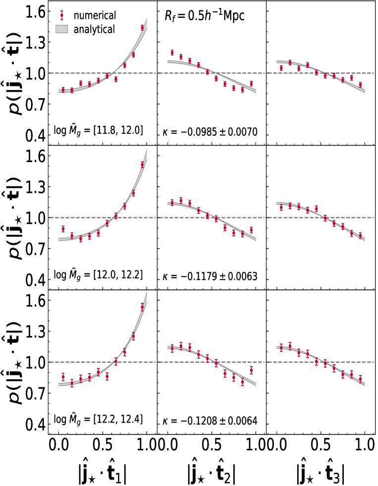
Figure 5: Analytic formula (gray areas) for the probability densities of the alignments between the present galaxy stellar spins and the three principal axes of the initial tidal field in three different mass ranges, compared with the numerical results (red filled circles) for the case of $R_{f}/(\,h^{-1}{\rm Mpc})=0.5$.

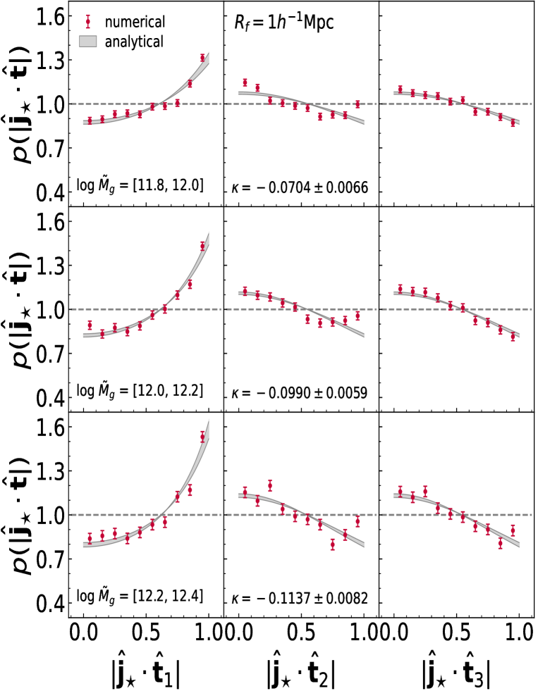
Figure 6: Same as Figure 5 but for the case of $R_{f}/(\,h^{-1}{\rm Mpc})=1$.

References

- Aragón-Calvo et al. (2007) Aragón-Calvo, M. A., van de Weygaert, R., Jones, B. J. T., et al. 2007, ApJ, 655, L5
- Ansar et al. (2023) Ansar, S., Kataria, S. K., & Das, M. 2023, MNRAS, 522, 2967. doi:10.1093/mnras/stad1060
- Bardeen et al. (1986) Bardeen, J. M., Bond, J. R., Kaiser, N., et al. 1986, ApJ, 304, 15. doi:10.1086/164143
- Bett et al. (2007) Bett, P., Eke, V., Frenk, C. S., et al. 2007, MNRAS, 376, 21
- Catelan & Theuns (1996) Catelan, P. & Theuns, T. 1996, MNRAS, 282, 436. doi:10.1093/mnras/282.2.436
- Chen et al. (2016) Chen, S., Wang, H., Mo, H. J., et al. 2016, ApJ, 825, 49. doi:10.3847/0004-637X/825/1/49
- Codis et al. (2012) Codis, S., Pichon, C., Devriendt, J., et al. 2012, MNRAS, 427, 3320. doi:10.1111/j.1365-2966.2012.21636.x
- Codis et al. (2015) Codis, S., Gavazzi, R., Dubois, Y., et al. 2015, MNRAS, 448, 3391
- Codis et al. (2018) Codis, S., Jindal, A., Chisari, N. E., et al. 2018, MNRAS, 481, 4753
- Coccato et al. (2009) Coccato, L., Gerhard, O., Arnaboldi, M., et al. 2009, MNRAS, 394, 1249. doi:10.1111/j.1365-2966.2009.14417.x
- Dubois et al. (2014) Dubois, Y., Pichon, C., Welker, C., et al. 2014, MNRAS, 444, 1453
- Forero-Romero et al. (2014) Forero-Romero, J. E., Contreras, S., & Padilla, N. 2014, MNRAS, 443, 1090
- Ganeshaiah Veena et al. (2018) Ganeshaiah Veena, P., Cautun, M., van de Weygaert, R., et al. 2018, MNRAS, 481, 414
- Ganeshaiah Veena et al. (2019) Ganeshaiah Veena, P., Cautun, M., Tempel, E., et al. 2019, MNRAS, 487, 1607. doi:10.1093/mnras/stz1343
- Ganeshaiah Veena et al. (2021) Ganeshaiah Veena, P., Cautun, M., van de Weygaert, R., et al. 2021, MNRAS, 503, 2280. doi:10.1093/mnras/stab411
- Hahn et al. (2007) Hahn, O., Carollo, C. M., Porciani, C., et al. 2007, MNRAS, 381, 41
- Herpich et al. (2015) Herpich, J., Stinson, G. S., Dutton, A. A., et al. 2015, MNRAS, 448, L99. doi:10.1093/mnrasl/slv006
- Herzog-Arbeitman et al. (2018) Herzog-Arbeitman, J., Lisanti, M., Madau, P., et al. 2018, Phys. Rev. Lett., 120, 041102. doi:10.1103/PhysRevLett.120.041102
- Kraljic et al. (2020) Kraljic, K., Davé, R., & Pichon, C. 2020, MNRAS, 493, 362. doi:10.1093/mnras/staa250
- Lee & Pen (2000) Lee, J. & Pen, U.-L. 2000, ApJ, 532, L5.
- Lee & Pen (2001) Lee, J. & Pen, U.-L. 2001, ApJ, 555, 106. doi:10.1086/321472
- Lee & Erdogdu (2007) Lee, J. & Erdogdu, P. 2007, ApJ, 671, 1248. doi:10.1086/523351
- Lee et al. (2018) Lee, J., Kim, S., & Rey, S.-C. 2018, ApJ, 860, 127. doi:10.3847/1538-4357/aac49c
- Lee (2019) Lee, J. 2019, ApJ, 872, 37. doi:10.3847/1538-4357/aafe11
- Lee et el. (2020) Lee, J., Libeskind, N. I., & Ryu, S. 2020, ApJ, 898, L27
- Lee & Libeskind (2020) Lee, J. & Libeskind, N. I. 2020, ApJ, 902, 22. doi:10.3847/1538-4357/abb314
- Lee et al. (2021) Lee, J., Moon, J.-S., Ryu, S., et al. 2021, ApJ, 922, 6.
- Lee et al. (2022) Lee, J., Moon, J.-S., & Yoon, S.-J. 2022, ApJ, 927, 29.
- Lee & Moon (2022) Lee, J. & Moon, J.-S. 2022, ApJ, 936, 119.
- Libeskind et al. (2013) Libeskind, N. I., Hoffman, Y., Forero-Romero, J., et al. 2013, MNRAS, 428, 2489
- Libeskind et al. (2018) Libeskind, N. I., van de Weygaert, R., Cautun, M., et al. 2018, MNRAS, 473, 1195. doi:10.1093/mnras/stx1976
- Lintott et al. (2008) Lintott, C. J., Schawinski, K., Slosar, A., et al. 2008, MNRAS, 389, 1179. doi:10.1111/j.1365-2966.2008.13689.x
- Marinacci et al. (2018) Marinacci, F., Vogelsberger, M., Pakmor, R., et al. 2018, MNRAS, 480, 5113
- Moon & Lee (2023) Moon, J.-S. & Lee, J. 2023, ApJ, 943, 13
- Motloch et al. (2021) Motloch, P., Yu, H.-R., Pen, U.-L., et al. 2021, Nature Astronomy, 5, 283. doi:10.1038/s41550-020-01262-3
- Motloch et al. (2022) Motloch, P., Pen, U.-L., & Yu, H.-R. 2022, Phys. Rev. D, 105, 083504. doi:10.1103/PhysRevD.105.083504
- Naiman et al. (2018) Naiman, J. P., Pillepich, A., Springel, V., et al. 2018, MNRAS, 477, 1206
- Nelson et al. (2018) Nelson, D., Pillepich, A., Springel, V., et al. 2018, MNRAS, 475, 624
- Nelson et al. (2019) Nelson, D., Springel, V., Pillepich, A., et al. 2019, Computational Astrophysics and Cosmology, 6, 2
- Paz et al. (2008) Paz, D. J., Stasyszyn, F., & Padilla, N. D. 2008, MNRAS, 389, 1127
- Pillepich et al. (2018) Pillepich, A., Nelson, D., Hernquist, L., et al. 2018, MNRAS, 475, 648
- Planck Collaboration et al. (2016) Planck Collaboration, Ade, P. A. R., Aghanim, N., et al. 2016, A&A, 594, A13
- Porciani et al. (2002a) Porciani, C., Dekel, A., & Hoffman, Y. 2002a, MNRAS, 332, 325. doi:10.1046/j.1365-8711.2002.05305.x
- Porciani et al. (2002b) Porciani, C., Dekel, A., & Hoffman, Y. 2002b, MNRAS, 332, 339. doi:10.1046/j.1365-8711.2002.05306.x
- Romanowsky et al. (2003) Romanowsky, A. J., Douglas, N. G., Arnaboldi, M., et al. 2003, Science, 301, 1696. doi:10.1126/science.1087441
- Springel et al. (2001) Springel, V., White, S. D. M., Tormen, G., et al. 2001, MNRAS, 328, 726
- Springel et al. (2018) Springel, V., Pakmor, R., Pillepich, A., et al. 2018, MNRAS, 475, 676
- Trowland et al. (2013) Trowland, H. E., Lewis, G. F., & Bland-Hawthorn, J. 2013, ApJ, 762, 72
- Wang et al. (2016) Wang, H., Mo, H. J., Yang, X., et al. 2016, ApJ, 831, 164. doi:10.3847/0004-637X/831/2/164
- Wang & Kang (2017) Wang, P. & Kang, X. 2017, MNRAS, 468, L123. doi:10.1093/mnrasl/slx038
- Wang et al. (2018) Wang, P., Guo, Q., Kang, X., et al. 2018, ApJ, 866, 138. doi:10.3847/1538-4357/aae20f
- White (1984) White, S. D. M. 1984, ApJ, 286, 38. doi:10.1086/162573
- Yu et al. (2019) Yu, H.-R., Pen, U.-L., & Wang, X. 2019, Phys. Rev. D, 99, 123532. doi:10.1103/PhysRevD.99.123532
- Yu et al. (2020) Yu, H.-R., Motloch, P., Pen, U.-L., et al. 2020, Phys. Rev. Lett., 124, 101302. doi:10.1103/PhysRevLett.124.101302
- Zhang et al. (2009) Zhang, Y., Yang, X., Faltenbacher, A., et al. 2009, ApJ, 706, 747. doi:10.1088/0004-637X/706/1/747
- Zhang et al. (2015) Zhang, Y., Yang, X., Wang, H., et al. 2015, ApJ, 798, 17. doi:10.1088/0004-637X/798/1/17
- Zhang et al. (2022) Zhang, B., Lee, K.-G., Krolewski, A., et al. 2022, arXiv:2211.09331 – subgrid physics