1

Deep Clustering with a Constraint for Topological Invariance based on Symmetric InfoNCE

Yuhui Zhang^1,∗, Yuichiro Wada^2,3,∗, Hiroki Waida^1,∗
Kaito Goto^1,†, Yusaku Hino^1,†, Takafumi Kanamori^1,3,‡
1Tokyo Institute of Technology, Tokyo, Japan
²Fujitsu Limited, Kanagawa, Japan
³RIKEN AIP, Tokyo, Japan

Keywords: Clustering, Deep Learning, Mutual Information, Contrastive Learning, Metric Learning

Abstract

We consider the scenario of deep clustering, in which the available prior knowledge is limited. In this scenario, few existing state-of-the-art deep clustering methods can perform well for both non-complex topology and complex topology datasets. To address the problem, we propose a constraint utilizing symmetric InfoNCE, which helps an objective of deep clustering method in the scenario train the model so as to be efficient for not only non-complex topology but also complex topology datasets. Additionally, we provide several theoretical explanations of the reason why the constraint can enhances performance of deep clustering methods. To confirm the effectiveness of the proposed constraint, we introduce a deep clustering method named MIST, which is a combination of an existing deep clustering method and our constraint. Our numerical experiments via MIST demonstrate that the constraint is effective. In addition, MIST outperforms other state-of-the-art deep clustering methods for most of the commonly used ten benchmark datasets.

1 Introduction

1.1 Background

Clustering is one of the most popular and oldest research fields of machine learning. Given unlabeled data points, the goal of clustering is to group them according to some criterion. In addition, in most of the cases clustering is performed with unlabeled datasets. Until today, many clustering algorithms have been proposed (MacQueen,, 1967; Day,, 1969; Girolami,, 2002; Wang et al.,, 2003; Ng et al.,, 2002; Ester et al.,, 1996; Sibson,, 1973). For a given unlabeled dataset, the number of clusters, and a distance metric, K-means (MacQueen,, 1967) aims to partition the dataset into the given number clusters. Especially when the squared Euclidean distance is employed as the metric, it returns convex-shaped clusters within short running time. GMMC (Gaussian Mixture Model Clustering) (Day,, 1969) assigns labels to estimated clusters after fitting GMM to an unlabeled dataset, where the number of clusters can be automatically determined by Bayesian Information Criterion (Schwarz,, 1978). The kernel K-means (Girolami,, 2002), kernel GMMC (Wang et al.,, 2003) and SC (Spectral Clustering) (Ng et al.,, 2002) can deal with more complicated shapes compared to K-means and GMMC. On the other hand, as examples categorized into a clustering method that does not require the number of clusters, DBSCAN (Ester et al.,, 1996) and Hierarchical Clustering (Sibson,, 1973) are listed.

Although the above-mentioned classical clustering methods are useful for low-dimensional small datasets, they often fail to handle large and high-dimensional datasets (e.g., image/text datasets). Due to the development of deep learning techniques for DNNs (Deep Neural Networks), we can now handle large datasets with high-dimension (Lecun et al.,, 2015). Note that a clustering method using DNNs is refereed to as Deep Clustering method.

1.2 Our Scenario with Deep Clustering

The most popular scenario for deep clustering is the domain-specific scenario (Scenario1) (Mukherjee et al.,, 2019; Ji et al.,, 2019; Asano et al.,, 2019; Van Gansbeke et al.,, 2020; Caron et al.,, 2020; Yang et al.,, 2020; Monnier et al.,, 2020; Li et al.,, 2021; Dang et al.,, 2021). In this scenario, an unlabeled dataset of a specific domain and its number of clusters are given, while specific rich knowledge in the domain can be available. The dataset is often represented by raw data. An example of the specific knowledge in the image domain is efficient domain-specific data-augmentation techniques (Ji et al.,, 2019). It is also known that CNN (Convolutional Neural Network) (LeCun et al.,, 1989) can be an efficient DNN to extract useful features from raw image data. In this scenario, most of the authors have proposed end-to-end methods, while some have done sequential methods. In the category of the end-to-end methods, a model is defined by an efficient DNN for a specific domain, where the input and output of the DNN are (raw) data and its predicted cluster label, respectively. The model is trained under a particular criterion as utilizing the domain-specific knowledge. In the category of the sequential methods, the clustering DNN is often constructed in the following three steps: 1) Create a DNN model that extracts features from data in a specific domain, followed by an MLP (Multi-Layer Perceptron) predicting cluster labels. 2) Train the feature-extracting DNN using an unlabeled dataset and domain-specific knowledge. Then, freeze the set of trainable parameters in the feature extracting DNN. 3) Train the MLP with the features obtained from the feature extracting DNN, and domain-specific knowledge.

The secondly important scenario is called the non-domain-specific scenario (Scenario2) (Springenberg,, 2015; Xie et al.,, 2016; Jiang et al.,, 2017; Guo et al.,, 2017; Hu et al.,, 2017; Shaham et al.,, 2018; Nazi et al.,, 2019; Gupta et al.,, 2020; McConville et al.,, 2020). In this scenario, an unlabeled dataset and the number of clusters are given, while a few generic assumptions for a dataset can be available, such as 1) the cluster assumption, 2) the manifold assumption, and 3) the smoothness assumption; see Chapelle et al., (2006) for details. In addition, unlabeled data is often represented by a feature vector. As well as Scenario1, many authors have proposed end-to-end methods where an MLP model is trained by utilizing some generic assumption, while some have done sequential methods.

A scenario apart from Scenario1 and Scenario2 is reviewed in Appendix A.1.

In this study, we focus on Scenario2 due to the following two reasons. The first reason is that we do not always encounter Scenario1 in practice. The second one is that if we prepare an efficient deep clustering algorithm of Scenario2, this algorithm can be incorporated into the third step of the sequential method of Scenario1.

1.3 Motivation behind and Goal

To understand the pros and cons of the recent state-of-the-art methods under Scenario2, we conduct preliminary experiments with eight deep clustering methods shown in Table 1. Among the eight methods, SCAN, IIC, CatGAN, and SELA are originally proposed in Scenario1. Therefore, we redefined the four methods to keep fairness in comparison; see Appendix E.3 for details of the alternative definitions that fit to our setting. For the datasets, we employed ten datasets as shown in the first row of Table 2. Here, Two-Moons and Two-Rings are synthetic, and the remaining eight are real-world; see more details in Section 4.2 and Appendix E.1. Throughout our experiments, we have found that the real-world datasets can be clustered well by performing K-means with the Euclidean distance, while the synthetic datasets cannot. We therefore regard the synthetic (resp. real-world) datasets as having complex topology (resp. non-complex topology). Intuitively, a dataset is topologically non-complex if it is clustered well by K-means with the Euclidean distance. Otherwise, the dataset is thought to have a complex topology. For more details of complex and non-complex topologies, see Appendix E.2.

Table 1: Representative deep clustering methods (either sequential or end-to-end). They are categorized into six types; $\mathfrak{T}_{1}$ to $\mathfrak{T}_{6}$. The example methods are shown for each type. Here, Seq. is abbreviation of the word ”Sequential”.

	Type	Explanation	Example(s)
Seq.	$\mathfrak{T}_{1}$	Plain embedding based	DEC (Xie et al.,, 2016), SCAN (Van Gansbeke et al.,, 2020)
	$\mathfrak{T}_{2}$	Spectral embedding based	SpectralNet (Shaham et al.,, 2018)
End-to-End	$\mathfrak{T}_{3}$	Variational bound based	VaDE (Jiang et al.,, 2017)
	$\mathfrak{T}_{4}$	Mutual information based	IMSAT (Hu et al.,, 2017), IIC (Ji et al.,, 2019)
	$\mathfrak{T}_{5}$	Generative adversarial net based	CatGAN (Springenberg,, 2015)
	$\mathfrak{T}_{6}$	Optimal transport based	SELA (Asano et al.,, 2019)

Table 2: Comparison of classical and deep clustering methods in terms of clustering accuracy (% One and seven trials are respectively conducted for the classical (top 3 methods) and the deep clustering methods, respectively. Mean and standard deviation of their accuracy are reported. Symbol ”-” means that result was not returned by the clustering algorithm within one hour of running. Numbers with $\dagger$ are copied from the corresponding studies. The symbol $\S$ means that an original method is redefined for Scenario2.

		Two-Moons	Two-Rings	MNIST	STL	CIFAR10	CIFAR100	Omniglot	20news	SVHN	Reuters10K
Classical Methods	K-means	75.1	50.0	53.2	85.6	34.4	21.5	12.0	28.5	17.9	54.1
	SC	100.0	100.0	63.7	83.1	36.6	-	-	-	27.0	43.5
	GMMC	85.9	50.3	37.7	83.5	36.7	22.5	7.6	39.0	14.2	67.7
Representative Existing Deep Methods	DEC	70.3(7.1)	50.7(0.3)	$\dagger$84.3	$\dagger$78.1(0.1)	$\dagger$46.9(0.9)	$\dagger$14.3(0.6)	$\dagger$5.7(0.3)	30.1(2.8)	$\dagger$11.9(0.4)	$\dagger$67.3(0.2)
	SpectralNet	100(0)	99.9(0.0)	$\dagger$82.6(3.0)	90.4(2.1)	44.3(0.6)	22.7(0.3)	2.5(0.1)	6.3(0.1)	10.4(0.1)	$\dagger$66.1(1.7)
	VaDE	50.0(0.0)	50.0(0.0)	83.0(2.6)	68.8(12.7)	39.5(0.7)	12.13(0.2)	1.0(0.0)	12.7(5.1)	32.9(3.2)	70.5(2.5)
	IMSAT	86.3(14.8)	71.3(20.4)	98.4(0.4)	93.8(0.5)	45.0(0.5)	27.2(0.4)	24.6(0.7)	37.4(1.4)	54.8(5.1)	72.7(4.6)
	IIC$\S$	77.2(18.4)	66.2(21.5)	45.4(8.3)	39.0(8.7)	23.9(4.8)	4.4(0.9)	2.3(0.4)	14.9(5.3)	17.1(1.1)	58.3(2.2)
	CatGAN$\S$	81.6(5.3)	53.7(2.5)	15.2(3.5)	32.9(3.0)	15.1(2.4)	5.1(0.5)	3.3(0.2)	19.5(6.5)	20.4(0.9)	43.6(7.3)
	SELA$\S$	62.7(9.5)	52.6(0.1)	46.1(3.4)	68.6(0.4)	29.7(0.1)	18.8(0.3)	11.3(0.2)	20.2(0.1)	19.3(0.3)	49.1(1.7)
	SCAN$\S$	85.7(22.6)	75.1(23.1)	82.1(3.7)	92.8(0.5)	43.3(0.6)	24.6(0.1)	17.6(0.4)	38.4(1.1)	23.2(1.6)	63.4(4.2)
	MIST via $\hat{I}_{\rm nce}$	100(0)	95.2(2.0)	98.0(1.0)	94.2(0.4)	48.9(0.7)	27.8(0.5)	24.0(1.0)	38.3(2.8)	58.7(3.5)	72.7(3.3)
	MIST (ours)	100(0)	93.3(16.3)	98.6(0.1)	94.5(0.1)	49.8(2.1)	27.8(0.5)	24.6(1.1)	38.8(2.3)	60.4(4.2)	73.4(4.6)

The experimental results are shown in Table 2. As shown in the table, for the complex topology datasets, all the eight deep clustering methods of Table 1 except for SpectralNet fail to cluster data points, compared to SC of a classical method. Note that, among the eight compared deep clustering methods, ones that incorporate the K-NN (K-Nearest Neighbor) graph tend to perform better for the complex topology datasets than ones that do not. Here, the methods incorporating the graph are SpectralNet, IMSAT, IIC, and SCAN. On the other hand, for the non-complex topology datasets, only IMSAT sufficiently outperforms the three classical methods on average. In addition, the average clustering performance of IMSAT over the ten datasets is the best among the eight methods. As Table 2 suggests, to the best of our knowledge, almost none of previous deep clustering methods sufficiently perform well for both non-complex and complex datasets. Those results motivate our study.

Our aim is to propose a constraint that helps an objective of deep clustering method in Scenario2 train the model so as to be efficient for not only non-complex topology but also complex topology datasets. Such a versatile deep clustering objective can be helpful for users.

1.4 Contributions

To achieve our goal, we propose the constraint for topological invariance. For two data points close to each other, the corresponding class probabilities computed by an MLP should be close. For example, in b) of Figure 1, any pair of two red points is close, while any pair of a red and a blue point are apart from each other. This constraint is introduced as a regularization based on the maximization of symmetric InfoNCE between the two probability vectors; see Section 3.3. In order to define the two probability vectors, we introduce two kinds of paired data. One is used for a non-complex topology dataset, which is based on a K-NN graph with the Euclidean metric; see Definition 3. The other is used for a complex topology dataset, and it is based on a K-NN graph with the geodesic metric on the graph; see Definition 4. Both graphs are defined only with an unlabeled dataset. The geodesic metric is defined by the graph-shortest-path distance on the K-NN graph constructed with the Euclidean distance.

We emphasize that under Scenario2, it is impossible to incorporate powerful domain-specific knowledge into a deep clustering method. In addition, the maximization of the symmetric InfoNCE has not been studied yet in the context of deep clustering. Moreover, we present the legitimacy of our topological invariant constraint by showing several theoretical findings from mainly two perspectives: 1) in Section 3.1, the motivations and the potential of the proposed constraint are clarified from the standpoint of statistical dependency measured by MI (Mutual Information), and 2) in Section 3.2, an extended result of the theory on contrastive representation learning derived from Wang et al., (2022) is presented to discuss advantages of the symmetric InfoNCE over InfoNCE for deep clustering. Note that InfoNCE (van den Oord et al.,, 2018) was ininitially used for domain-specific representation learning such as vision tasks, NLP, and reinforcement learning. Here, a purpose of representation learning is to extract useful features that can be applied to a variety range of machine learning methods (Bengio et al.,, 2013). Whereas, the purpose of clustering is to annotate the cluster labels to unlabeled data points.

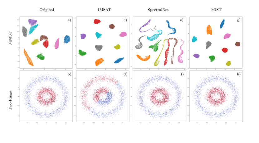
Figure 1: Two-dimensional visualizations of clustering results. In the first row except for a), three visualizations are obtained via the following procedure: using the trained MLP, compute the output for each feature in MNIST, where dimension of the feature is 784. Then, the outputs are transformed into two-dimensional vectors by UMAP. Thereafter, true labels are assigned to those vectors. As for a), the original features are directly transformed into two-dimensional vectors by UMAP, and then the labels are assigned to the transformed vectors. For the second row, the true labels (resp. predicted cluster labels by the trained MLP) are assigned to the original features for obtaining b) (resp. d), f), and h)). Note that the original features of Two-Rings belong to $\mathbb{R}^{2}$.

The main contributions are summarized as follows:

1. We propose a topological invariant constraint via the symmetric InfoNCE for the purpose of deep clustering in Scenario2, and then show the advantage by providing analysis from several theoretical aspects.

2. To evaluate the proposed constraint in numerical experiments, by applying the constraint to IMSAT, we define a deep clustering method named MIST (Mutual Information maximization with local Smoothness and Topologically invariant constraints). In the experiments, we confirm that the proposed constraint enhances the accuracy of a deep clustering method. Furthermore, to the best of our knowledge, MIST achieves state‐of‐the‐art clustering accuracy in Scenario2 for not only non-complex topology datasets but also complex topology datasets.

In Figure 1, a positive impact of the topological invariant constraint toward IMSAT is visualized via UMAP (McInnes et al.,, 2018); compare d) and h) in the figure. See further details of Figure 1 and more two-dimensional visualizations of MIST for other datasets in Appendix E.4.

This paper is organized as follows. In Section 2, we overview related works. In Section 3, we explain details of the topological invariant constraint, and then show the theoretical properties. In numerical experiments of Section 4, we define MIST. Then, we evaluate the proposed constraint via MIST using two synthetic datasets and eight real-world datasets. In the same section, some case studies are also provided. In Section Conclusion, we conclude this paper.

2 Related Works

In Section 2.1, we briefly explain representative deep clustering methods shown as examples in Table 1 since they are compared methods in numerical experiments of Section 4. Then, details of InfoNCE, which is closely related to our topological invariant constraint, is introduced in Section 2.2.

2.1 Representative Deep Clustering Methods

Let us start from sequential methods of $\mathfrak{T}_{1}$ and $\mathfrak{T}_{2}$ in Table 1. In DEC (Xie et al.,, 2016) of $\mathfrak{T}_{1}$, at first, a stacked denoising Auto-Encoder (AE) is trained with a set of unlabeled data points to extract the feature. Using the trained encoder, we can have the feature vectors. Then, K-means is used on the vectors in order to obtain the set of centroids. After that, being assisted by the centroids, the encoder is refined for the clustering. In SCAN (Van Gansbeke et al.,, 2020) of $\mathfrak{T}_{1}$, a ResNet (He et al.,, 2016) is trained using augmented raw image datasets under SimCLR (Chen et al.,, 2020) criterion to extract the features. Then, the clustering MLP added to the trained ResNet is tuned by maximizing Shannon-entropy of the cluster label while two data points in a nearest neighbor relationship are forced to have same cluster label. Then, in SpectralNet (Shaham et al.,, 2018) of $\mathfrak{T}_{2}$, at first, a Siamese network is trained by the predefined similarity scores on the K-NN graph. Then, being assisted by the trained Siamese network, a clustering DNN is trained. Note that the two networks (i.e., Siamese net and clustering net) are categorized into this method.

With regard to end-to-end methods of $\mathfrak{T}_{3}$ to $\mathfrak{T}_{6}$, in VaDE (Jiang et al.,, 2017) of $\mathfrak{T}_{3}$, a variational AE is trained so that the latent representation of unlabeled data points has the Gaussian mixture distribution. Here, the number of mixture components is equal to the number of clusters. For IMSAT and IIC of $\mathfrak{T}_{4}$, in IMSAT (Hu et al.,, 2017), the clustering model is trained via maximization of the MI between a data point and the cluster label, while regularizing the model to be locally smooth; see Appendix A.3. Likewise, IIC (Ji et al.,, 2019) returns the estimated cluster labels using the trained model for clustering. The training criterion is based on maximization of the MI between the cluster label of a raw image and the cluster label of the transformed raw image; see Appendix A.2. IIC employs a CNN-based clustering model to take advantages of image-specific prior knowledge. Furthermore, in CatGAN (Springenberg,, 2015) of $\mathfrak{T}_{5}$, the neural network for clustering is trained to be robust against noisy data. Here, the noisy data is defined as a set of fake data points obtained from the generator that is trained to mimic the distribution of original data. Lastly, in SELA (Asano et al.,, 2019) of $\mathfrak{T}_{6}$, a ResNet is trained for clustering using an augmented unlabeled dataset with pseudo labels under the cross-entropy minimization criterion. The pseudo labels are updated at the end of every epoch by solving an optimal transporting problem.

2.2 Info Noise Contrastive Estimation

In representation learning, InfoNCE (Info Noise Contrastive Estimation) based on NCE has recently become a popular objective. The ($q$-)InfoNCE of the random variables $Z$ and $Z^{\prime}$ is defined by

$$I_{\mathrm{nce},q}(Z;Z^{\prime})=\mathbb{E}[q(Z,Z^{\prime})]-\mathbb{E}_{Z}\big{[}\log\mathbb{E}_{Z^{\prime}}[e^{q(Z,Z^{\prime})}]\big{]},$$ (1)

where $q$ is called critic function that quantifies the dependency between $Z$ and $Z^{\prime}$. For any critic, $q$-InfoNCE provides a lower bound of an MI. Furthermore, we can see that the maximum value of $I_{\mathrm{nce},q}$ is the MI, which is attained by $q(z,z^{\prime})=\log p(z|z^{\prime})+[\text{any function of $z$}]$; see Poole et al., (2019); Belghazi et al., (2018) and Eq.(16) for details. Here, $p(z|z^{\prime})$ is the conditional probability of $z$ given $z^{\prime}$. When it comes to the image processing (Chen et al.,, 2020; Grill et al.,, 2020), the observations, $z$ and $z^{\prime}$, are often given as different views or augmentations of an image. For example, $z$ and $z^{\prime}$ are observed by rotating, cropping, or saturating the same source image. Such a pair of images are regarded as positive samples (pair). A pair of transformed images coming from different source images are negative samples (pair).

Suppose we have samples $z_{1},\cdots,z_{m}$ and $z_{1}^{\prime},\cdots,z_{m}^{\prime}$, such that $z_{i}$ and $z_{i}^{\prime}$ are all positive samples for $i=1,\cdots,m$ and $z_{i}$ and $z_{j}^{\prime}$ for $i\neq j$ are negative samples. Then, InfoNCE is empirically approximated by

$$\hat{I}_{\text{nce},q}=\frac{1}{m}\sum_{i=1}^{m}\log\frac{e^{q\left(z_{i},z^{\prime}_{i}\right)}}{\frac{1}{m}\sum_{j=1}^{m}e^{q\left(z_{i},z_{j}^{\prime}\right)}}.$$ (2)

In order to approximate the MI by InfoNCE, one can use a parameterized model with a critic function $q$. In the original work of InfoNCE (van den Oord et al.,, 2018) the critic $q_{W}(z,z^{\prime})=z^{T}Wz^{\prime}$ with the weight matrix $W$ is employed. Then, the maximum value of $\hat{I}_{\text{nce},q_{W}}$ w.r.t. $W$ is computed to estimate the MI. As pointed out by van den Oord et al., (2018); Poole et al., (2019); Tschannen et al., (2019), The empirical InfoNCE is bounded above by $\log m$, making the bound loose when $m$ is small, or the MI $I(Z;Z^{\prime})$ is large.

3 Proposed Constraint and its Theoretical Analysis

3.1 Notations

In the following, $\mathcal{D}=\{x_{i}\}_{i=1}^{n}$ ($\forall i;x_{i}\in\mathbb{R}^{d}$) is a set of unlabeled data, where $n$ is the number of data points and $d$ is the dimension of a data point. The number of clusters is denoted by $C$. Here, let $y_{i}$ denote the true label of $x_{i}$. Let us define $p\left(y|x\right)$ as the conditional discrete probability of a cluster label $y\in\{1,2,...,C\}$ for a data point $x\in\mathbb{R}^{d}$. The random variable corresponding to $x$ (resp. $y$) is denoted by $X$ (resp. $Y$). Let $\Delta^{C-1}=\{z\in\mathbb{R}^{C}\;|\;z\geq 0,z^{\top}\mathbf{1}=1\}$ be the $(C-1)$-dimensional probability simplex, where $\mathbf{1}$ is the $C$-dimensional vector $(1,1,...,1)^{\top}$.

Definition 1 (MLP model $g_{\theta}$)

Consider a DNN model $g_{\theta}(x):\mathbb{R}^{d}\to\Delta^{C-1}$ with trainable set of parameters $\theta$, where the activation for the last layer is defined by the $C$-dimensional softmax function. The $y$-th element of $g_{\theta}(x)$ is denoted by $g_{\theta}^{y}(x)$. Let $\theta^{\ast}$ denote the trained set of parameters via a clustering objective, using an unlabeled dataset $\mathcal{D}$. The predicted cluster label of $x_{i}\in\mathcal{D}$ is defined by $\hat{y}_{i}={\rm argmax}_{y\in\{1,\cdots,C\}}g_{\theta^{\ast}}^{y}(x_{i})$.

3.2 Preliminary

Consider Scenario2 of Section 1.2, where a set of unlabeled data $\mathcal{D}=\{x_{i}\}_{i=1}^{n},x_{i}\in\mathbb{R}^{d}$ and the number of clusters $C$ are given, while a few generic assumptions for the dataset can be available. We firstly in Section 3.3 introduce the topological invariant constraint based on symmetric InfoNCE and an MLP model $g_{\theta}$. Then, in Section 3.4, some relations between the symmetric InfoNCE and the corresponding MI are theoretically analyzed. Thereafter, based on the analysis, we explain theoretical advantages of the symmetric InfoNCE over existing popular constraints such as IIC and InfoNCE in terms of deep clustering.

Before stating the mathematical definitions and the properties, we briefly explain why the symmetric InfoNCE can enhance a deep clustering method as a topological invariant constraint. As mentioned in Section 1.4, the topological invariant constraint is expected to regularize $g_{\theta}$ so as to be $g_{\theta}(X)\approx g_{\theta}(X^{\prime})\in\Delta^{C-1}$ for any geodesically-close two data points $X,X^{\prime}\in\mathcal{D}$ in the original space $\mathbb{R}^{d}$. In other words, predicted cluster labels of $X$ and $X^{\prime}$ are enforced to be same. For the regularization, InfoNCE and its variants are potentially useful. The reason is that in representation learning InfoNCE is empirically successful for making the following two feature vectors close to each other: 1) a feature vector returned by a DNN with a raw data as an input, 2) a feature returned by the same DNN with an augmented data from the raw data (van den Oord et al.,, 2018; Chen et al.,, 2020). Note that feature vectors described in 1) and 2) are not in $\Delta^{C-1}$ but usually in the high-dimensional Euclidean space. In this study, the symmetric InfoNCE between $X$ and $X^{\prime}$ is proposed as a constraint for topological invariance. The pair $(X,X^{\prime})$ is given by $(X,T(X))$, where $T(X)$ is a transformation of $X$: some practical tranformations are introduced in Definition 3 and 4 of Section 3.3.

3.3 Topological Invariant Constraint

We aim to design a constraint for topological invariance that should satisfy the following condition; if clusters of $\mathcal{D}$ have a non-complex (resp. complex) topology, the constraint assists a model $g_{\theta}$ to predict the same cluster labels for $x\in\mathcal{D}$ and $x^{\prime}\in\mathcal{D}$ whenever $x$ and $x^{\prime}$ are close to each other in terms of the Euclidean (resp. geodesic) distance. In the sequel, we define the constraint via symmetric InfoNCE. Then, we investigate its theoretical properties.

Firstly, let us define a function $q:\Delta^{C-1}\times\Delta^{C-1}\to\mathbb{R}$ as follows:

$$q(z,z^{\prime})=\log\left(\exp_{\alpha}\big{(}\tau(z^{\top}z^{\prime}-1)\big{)}\right),$$ (3)

where $\alpha\in\mathbb{R}$ and $0\leq\tau\leq|1-\alpha|^{-1}$. In addition, for $u\in\mathbb{R}$, $\exp_{\alpha}(u)$ is defined by $[1+(1-\alpha)u]_{+}^{1/(1-\alpha)}$ for $\alpha\neq 1$ and $e^{u}$ for $\alpha=1$, where $[\;\cdot\;]_{+}=\max\{\cdot,0\}$. The function $q$ of Eq.(3) w.r.t. $z$ and $z^{\prime}$ is maximized if and only if $z$ and $z^{\prime}$ are the same one-hot vector. On the other hand, it is minimized if and only if $z^{\top}z^{\prime}=0$ (i.e., $z$ and $z^{\prime}$ are orthogonal to each other).

We then define transformation $T$ for constructing a pair of geodesically-close two data points $(X,T(X))$ based on $X$ as follows.

Definition 2 (Transformation $T$)

Let $X$ be a $d$-dimensional random variable. Then, $T:\mathbb{R}^{d}\to\mathbb{R}^{d}$ denote the transformation of $X$, and it is also a random variable. The realization is denoted by $t:\mathbb{R}^{d}\to\mathbb{R}^{d}$. Given a data point $x$, the function $t$ is sampled from the conditional probability $p(t|x)$.

The probability $p(t|x)$ is defined through a generative process. In this study, two processes, $\mathcal{T}_{\mathfrak{e}}$ and $\mathcal{T}_{\mathfrak{g}}$, are considered. The first (resp. second) one, $\mathcal{T}_{\mathfrak{e}}$ (resp. $\mathcal{T}_{\mathfrak{g}}$), is defined using the K-NN graph with the Euclidean (resp. geodesic) distance, and is employed for non-complex (resp. complex) topology datasets.

Definition 3 (Generative process $\mathcal{T}_{\mathfrak{e}}$)

Given an unlabeled dataset $\mathcal{D}=\{x_{i}\}_{i=1}^{n}$, a natural number $K_{0}$, and $\beta\in[0,1)$ as inputs, then the generative process of a transformation is defined as follows. 1) At the beginning, build a K-NN graph with $K=K_{0}$ on $\mathcal{D}$ based on the Euclidean distance. 2) For all $k=1+\lfloor\beta K_{0}\rfloor,\cdots,K_{0}$, define a function $t^{(i\to k)}:\mathbb{R}^{d}\to\mathbb{R}^{d}$ by $x^{(k)}_{i}=t^{(i\to k)}(x_{i})$, where $x^{(k)}_{i}$ is a $k$-th nearest neighbor data points of $x_{i}$ on the graph. 3) Define the conditional distribution $p(t|x_{i})$ as the uniform distribution on $t^{(i\to k)},k=1+\lfloor\beta K_{0}\rfloor,\cdots,K_{0}$.

Definition 4 (Generative process $\mathcal{T}_{\mathfrak{g}}$)

Given an unlabeled dataset $\mathcal{D}=\{x_{i}\}_{i=1}^{n}$, a natural number $K_{0}$, and $\beta\in[0,1)$ as inputs, then firstly build a K-NN graph based on the Euclidean distance with $K=K_{0}$ on $\mathcal{D}$. Then, in order to approximate the geodesic distance between $x_{i}$ and $x_{j}$, compute the graph-shortest-path distance. Let $\mathfrak{g}_{ij}$ be the approximated geodesic distance between $x_{i}$ and $x_{j}$, and $\mathfrak{G}$ be an $n\times n$ matrix $(\mathfrak{g}_{ij})_{i,j=1,\cdots,n}$. For each $i$, let $\mathcal{M}_{i}=\{j\;|\;0<\mathfrak{g}_{ij}<\infty\}$ be the set of indices whree each $x_{j}$ is a neighborhood of $x_{i}$ under the geodesic distance. For each $i$, the generative process of the transformation $t$ is given as follows. 1) For all $k=|\mathcal{M}_{i}|-\lfloor\beta K_{\mathfrak{g}}\rfloor+1,\cdots,|\mathcal{M}_{i}|$, define a function $t^{(i\to k)}:\mathbb{R}^{d}\to\mathbb{R}^{d}$ by $x^{(k)}_{i}=t^{(i\to k)}(x_{i})$, where $x^{(k)}_{i}$ is a $k$-th geodesically nearest neighbor data points from $x_{i}$ on $\mathfrak{G}$ except in the case of $\mathfrak{g}_{ij}=\infty$ and $\mathfrak{g}_{ij}=0$. 2) Define the conditional distribution $p(t|x_{i})$ as the uniform distribution on $t^{(i\to k)},k=|\mathcal{M}_{i}|-\lfloor\beta K_{\mathfrak{g}}\rfloor+1,\cdots,|\mathcal{M}_{i}|$.

The time and memory complexities with $\mathcal{T}_{\mathfrak{e}}$ and $\mathcal{T}_{\mathfrak{g}}$ are provided in Appendix D.2. Intuitively, when $\beta=0$, $\mathcal{T}_{\mathfrak{e}}$ picks a random neighbor of $x$ as $T(x)$ in the $K_{0}$-nearest neighbor graph, while $\mathcal{T}_{\mathfrak{g}}$ picks the a random neighbor by the geodesic metric induced by the $K_{0}$-nearest neighbor graph. Larger $\beta$ disables $\mathcal{T}_{\mathfrak{e}}$ and $\mathcal{T}_{\mathfrak{g}}$ from picking closest neighbors.

Using the function $q$ of Eq.(3), let us define $I_{\rm nce}\equiv I_{\mathrm{nce},q}(g_{\theta}(X);g_{\theta}(T(X)))$ and $I^{\prime}_{\rm nce}\equiv I_{\mathrm{nce},q}(g_{\theta}(T(X));g_{\theta}(X))$; see $I_{{\rm nce},q}$ in Eq.(1). We then define the symmetric InfoNCE by $\left(I_{\mathrm{nce}}+I^{\prime}_{\mathrm{nce}}\right)/2$. Then, the topological invariant constraint is defined as follows:

$$-M\leq-\frac{I_{\mathrm{nce}}+I^{\prime}_{\mathrm{nce}}}{2}\leq-M+\delta,$$ (4)

where $\delta$ is a small fixed positive value, and $M=\sup_{\theta}\left(I_{\mathrm{nce}}+I^{\prime}_{\mathrm{nce}}\right)/2$.

In practice, given a mini-batch $\mathcal{B}\subseteq\mathcal{D}$, we can approximate $-\left(I_{\mathrm{nce}}+I^{\prime}_{\mathrm{nce}}\right)/2$ by $-(\hat{I}_{\text{nce}}+\hat{I}^{\prime}_{\text{nce}})/2$ (recall Eq.(2) for $\hat{I}_{\rm nce}$), where $-\hat{I}_{\text{nce}}$ is given by

$$-\hat{I}_{\text{nce}}=-\frac{1}{|\mathcal{B}|}\sum_{x_{i}\in\mathcal{B}}\log\frac{e^{q\left(g_{\theta}(x_{i}),g_{\theta}\left(t_{i}(x_{i})\right)\right)}}{\frac{1}{|\mathcal{B}|}\sum_{x_{j}\in\mathcal{B}}e^{q\left(g_{\theta}(x_{i}),g_{\theta}\left(t_{j}(x_{j})\right)\right)}}$$ (5)

with the sampled transformation function $t_{i}$ from $p(t|x_{i})$ and $-\hat{I}^{\prime}_{\text{nce}}$ is given by switching two inputs in the function $q$ of Eq.(5). Here, $|\mathcal{B}|$ denotes the cardinality of $\mathcal{B}$.

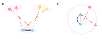
Figure 2: Illustration of the effect by minimizing point-wise positive loss $\ell_{\rm ps}(x_{i})$ and point-wise negative loss $\ell_{\rm ng}(x_{i})$. In both i) and ii), the colors (blue, magenta, and yellow) mean different labels, and the light-colored manifolds express true clusters. For i) (resp. ii)), the set of clusters builds Three-Blobs (resp. Two-Rings), and it is an example of non-complex (resp. complex) topology datasets. A pair of the small circle and triangle symbols with the same color means a pair of a data point $x$ and the transformed data point $t(x)$, where such pair is constructed by $\mathcal{T}_{\mathfrak{e}}$ of Definition 3 (resp. $\mathcal{T}_{\mathfrak{g}}$ of Definition 4) in i) (resp. ii)). The two data points connected by the red dash line (resp. blue straight or curved line) are enforced to be distant (resp. close) to each other by minimizing $\ell_{\rm ng}(x_{i})$ (resp. $\ell_{\rm ps}(x_{i})$).

To understand the above empirical symmetric InfoNCE more, we decompose $-(\hat{I}_{\text{nce}}+\hat{I}^{\prime}_{\text{nce}})/2$ into the following three terms:

$$\begin{split}-\log|\mathcal{B}|\underbrace{-\frac{1}{|\mathcal{B}|}\sum_{x_{i}\in\mathcal{B}}q\left(g_{\theta}(x_{i}),g_{\theta}\left(t_{i}(x_{i})\right)\right)}_{\text{$L_{\rm ps}$: positive loss}}\underbrace{+\frac{1}{|\mathcal{B}|}\sum_{x_{i}\in\mathcal{B}}\frac{1}{2}\log\left(\sum_{x_{j}\in\mathcal{B}}\sum_{x_{i^{\prime}}\in\mathcal{B}}e^{a\left(i,i^{\prime},j\right)}\right)}_{\text{$L_{\rm ng}$: negative loss}},\end{split}$$ (6)

where $a\left(i,i^{\prime},j\right)=q\left(g_{\theta}(x_{i}),g_{\theta}\left(t_{j}(x_{j})\right)\right)+q\left(g_{\theta}(x_{i^{\prime}}),g_{\theta}\left(t_{i}(x_{i})\right)\right)$. Note that the decomposition is based on the fact that $q(z,z^{\prime})=q(z^{\prime},z)$ for all $z,z^{\prime}\in\Delta^{C-1}$. In Eq.(6), we call the second and the third term positive loss and negative loss, respectively. These names are natural in the sense of metric learning (Sohn,, 2016). Indeed, making $L_{\rm ps}$ smaller w.r.t. $\theta$ leads to $g_{\theta}(x_{i})\approx g_{\theta}\left(t_{i}(x_{i})\right)$ for all $i$ due to the definition of $q$. Thus, since $t_{i}(x_{i})$ is a neighbor data point of $x_{i}$, via minimization of $L_{\rm ps}$, the model predicts the same cluster labels for $x_{i}$ and $t_{i}(x_{i})$. Here, the neighborhood is defined with the Euclidean (resp. the geodesical) neighborhood on K-NN graph of $\mathcal{D}$ through $\mathcal{T}_{\mathfrak{e}}$ (resp. $\mathcal{T}_{\mathfrak{g}}$). On the other hand, making $L_{\rm ng}$ smaller leads to $g_{\theta}(x_{i})\neq g_{\theta}\left(t_{j}(x_{j})\right)$ for all $i,j$ and $g_{\theta}(x_{i^{\prime}})\neq g_{\theta}\left(t_{i}(x_{i})\right)$ for all $i^{\prime}$ and $i$ due to the definition of $q$. Thus, via minimization of $L_{\rm ng}$, the model can return non-degenerate clusters (i.e., not all the predicted cluster labels are the same).

In Figure 2, for simplicity, we illustrate effects brought by minimizing point-wise positive loss $\ell_{\rm ps}(x_{i})$ and point-wise negative loss $\ell_{\rm ng}(x_{i})$, which are defined in Eq.(6) as follows; $\ell_{\rm ps}(x_{i})=-q\left(g_{\theta}(x_{i}),g_{\theta}\left(t_{i}(x_{i})\right)\right),\;\ell_{\rm ng}(x_{i})=\frac{1}{2}\log\left(\sum_{x_{j}\in\mathcal{B}}\sum_{x_{i^{\prime}}\in\mathcal{B}}e^{a\left(i,i^{\prime},j\right)}\right).$

3.4 Theoretical Analysis

In this section, we investigate theoretical properties of the symmetric InfoNCE loss. In Section 3.1, we study the relationship between MI and symmetric InfoNCE. In Section 3.2, we show a theoretical difference between InfoNCE and symmetric InfoNCE.

3.1 Relationship between Symmetric InfoNCE and MI

First we make clear the reason for selecting Eq.(3) as a critic function. Our explanation begins by deriving the optimal critic of the symmetric InfoNCE loss.

Proposition 1

Let $Z$ and $Z^{\prime}$ denote two random variables having the joint probability density $p$. Let $I_{\mathrm{nce},q}(Z;Z^{\prime})$ the InfoNCE loss defined in Eq.(1). Let us define $I_{\mathrm{nce},q}(Z^{\prime};Z)$ by switching $Z$ and $Z^{\prime}$ of $I_{\mathrm{nce},q}(Z;Z^{\prime})$. Then, the following MI, $I(Z;Z^{\prime}):=\mathbb{E}_{p(Z,Z^{\prime})}\left[\log\frac{p(Z,Z^{\prime})}{p(Z)p(Z^{\prime})}\right],$ is an upper bound of the symmetric InfoNCE, $\frac{I_{\mathrm{nce},q}(Z;Z^{\prime})+I_{\mathrm{nce},q}(Z^{\prime};Z)}{2}$. Moreover, if the function $q$ satisfies

$$q(z,z^{\prime})=\log{\frac{p(z,z^{\prime})}{p(z)p(z^{\prime})}}+c,\,c\in\mathbb{R},$$ (7)

then the equality $I(Z;Z^{\prime})=\frac{I_{\mathrm{nce},q}(Z;Z^{\prime})+I_{\mathrm{nce},q}(Z^{\prime};Z)}{2}$ holds. In other words, $q$ satisfying Eq.(7) is the optimal critic.

The proof is shown in Appendix B.1.

Consider $g_{\theta}(X)$ and $g_{\theta}(T(X))$ as $Z$ and $Z^{\prime}$ of Proposition 1, respectively. Then, the symmetric InfoNCE $\left(I_{\mathrm{nce}}+I^{\prime}_{\mathrm{nce}}\right)/2$ of Eq.(4) can be upper-bounded by

$$I(g_{\theta}(X);g_{\theta}(T(X))).$$ (8)

Thus, maximization of the symmetric InfoNCE (i.e., the constraint of Eq.(4)) is a reasonable approach to maximize the MI. Note that the computation of $I(g_{\theta}(X);g_{\theta}(T(X)))$ is difficult, since density-estimation on $\Delta^{C-1}$ is required.

It is interesting that the optimal critic of the symmetric InfoNCE loss is the pointwise MI of $g_{\theta}(X)$ and $g_{\theta}(T(X))$ up to an additive constant. Moreover, we remark that the function $q$ of Eq.(3) is in fact designed based on the optimal critic, Eq.(7), of the symmetric InfoNCE. As shown in the equation, the optimal critic of the symmetric InfoNCE is $q^{\ast}(z,z^{\prime})=\log\frac{p(z,z^{\prime})}{p(z)p(z^{\prime})}+c,c\in\mathbb{R}$. Thus, the joint probability density $p(z,z^{\prime})$ is expressed by $p(z,z^{\prime})\propto p(z)p(z^{\prime})e^{q^{\ast}(z,z^{\prime})}$. Hence, the critic function adjusts the statistical dependency between $z$ and $z^{\prime}$. In our study, we suppose that $z,z^{\prime}\in\Delta^{C-1}$, and the critic $q(z,z^{\prime})$ is expressed as an increasing function of $z^{\top}z^{\prime}$. When $z$ and $z^{\prime}$ are both the same one-hot vector in $\Delta^{C-1}$, $p(z,z^{\prime})$ is assumed to be large. On the other hand, if $z^{\top}z^{\prime}=0$, $p(z,z^{\prime})$ is assumed to take a small value. We also introduce a one-dimensional parameter $\alpha$ for the critic $q_{\alpha}$ to tune the intensity of the dependency. Although there are many choices of critic functions, we here employ the $\alpha$-exponential function, because $\exp_{\alpha}$ can express a wide range of common probabilities in statistics only by one parameter; see details of $\alpha$-exponential function in Naudts, (2009); Amari and Ohara, (2011); Matsuzoe and Ohara, (2012). Eventually, the model of the critic is given by $p_{\alpha}(z,z^{\prime})\propto p(z)p(z^{\prime})\exp_{\alpha}\big{(}\tau(z^{\top}z^{\prime}-1)\big{)}$, where $\alpha\in\mathbb{R}$ and $0\leq\tau\leq|1-\alpha|^{-1}$. Note that the normalization constant of $p_{\alpha}$ is no need when we compute the symmetric InfoNCE. In our experiments, we consider both $\alpha$ and $\tau$ as the hyper-parameters.

Remark 1

The cosine-similarity function $s(z,z^{\prime})=z^{\top}z^{\prime}/\|z\|_{2}\|z^{\prime}\|_{2},z,z^{\prime}\in\Delta^{C-1}$ is commonly used in the context of representation learning (Chen et al.,, 2020; Bai et al.,, 2021). However, we do not use the cosine-similarity function as the critic function $q$ in Eq.(3). This is because in our problem the cosine-similarity function is not relevant to estimate the one-hot vector by the model $g_{\theta}(x)$. Indeed, for $q(z,z^{\prime})=s(z,z^{\prime})$ and $C=2$, the pair $(z,z^{\prime})$ satisfying $z=z^{\prime}=(1/2,1/2)^{\top}\in\Delta^{C-1}$ is a maximizer of $q(z,z^{\prime})$, i.e., there exists a pair of non-one-hot vectors $z$ and $z^{\prime}$ that minimizes $L_{\rm ps}$ in Eq.(6).

Next, we investigate a few more properties of the symmetric InfoNCE loss from the perspective of MI. First we present a theoretical comparison between the symmetric InfoNCE loss and IIC (see IIC in Section 2.1 and Appendix A.2).

Proposition 2

Consider a feature $X$ and its transformation function $T$ of Definition 2. Let $Y$ (resp. $Y^{\prime}$) denote a cluster label of $X$ (resp. $T(X)$). Then, the following inequality holds:

$$I(Y;Y^{\prime})\leq I(g_{\theta}(X);g_{\theta}(T(X))),$$ (9)

where $g_{\theta}$ is the same model as introduce in Definition 1.

The proof is shown in Appendix B.2.

The above data processing inequality guarantees that $I(g_{\theta}(X);g_{\theta}(T(X)))$ brings richer information than $I(Y;Y^{\prime})$ used in IIC. Since our constraint is related to $I(g_{\theta}(X);g_{\theta}(T(X)))$, Eq.(9) indicates the advantage of ours over IIC. To discuss the consequence of Proposition 2 in more detail, we provide a statistical analysis on the gap between the following two quantities:

• The maximum value $I(g_{\theta}(X);g_{\theta}(T(X)))$ w.r.t. $\theta$,

• The mutual information evaluated at $\widehat{\theta}$, where $\widehat{\theta}$ is the parameter maximizing the empirical symmetric InfoNCE.

To the best of our knowledge, such statistical analysis is not provided in previous theoretical studies related to InfoNCE.

Theorem 1 (Informal version)

Consider the empirical symmetric InfoNCE of Section 3.3 with a critic $q\in\mathcal{Q}$ for a dataset $\mathcal{D}=\{x_{i}\}_{i=1}^{n}$. Here, $\mathcal{Q}$ is a set of critics defined as follows: $\mathcal{Q}=\{\phi_{(\alpha,\tau)}\,:\,(\alpha,\tau)\in\Xi\}$, where $\phi_{(\alpha,\tau)}(z^{\top}z^{\prime})=\log\left(\exp_{\alpha}\big{(}\tau(z^{\top}z^{\prime}-1)\big{)}\right)$ (see Eq.(3)), and $\Xi$ is a set of all possible $(\alpha,\tau)$ pairs. Let $\widehat{I}_{\mathrm{sym\_nce},q}(\theta)$ denote the empirical symmetric InfoNCE, where $\theta$ is a set of parameters in $g_{\theta}$ of Definition 1. Let us define $\widehat{\theta}$ by $\widehat{\theta}=\arg\max_{\theta}\sup_{q\in\mathcal{Q}}\widehat{I}_{\mathrm{sym\_nce},q}(\theta).$ We define $\theta^{*}$ as the maximizer of $I(g_{\theta}(X);g_{\theta}(T(X)))$ w.r.t $\theta$. Suppose that $0\leq\delta$ is a constant. Then, with the probability greater than $1-\delta$, the gap between $I(g_{\theta^{*}}(X);g_{\theta^{*}}(T(X)))$ and $I(g_{\widehat{\theta}}(X);g_{\widehat{\theta}}(T(X)))$ is given by

$$\begin{split}&\phantom{\leq}I(g_{\theta^{*}}(X);g_{\theta^{*}}(T(X)))-I(g_{\widehat{\theta}}(X);g_{\widehat{\theta}}(T(X)))\\ &\leq\mathrm{(Approx.~{}Err.)}+(\mathrm{Gen.~{}Err.})+c\,\sqrt{\frac{\log(1/\delta)}{n}},\end{split}$$ (10)

where $c>0$ is a constant, and Approx. Err. (resp. Gen. Err.) is short for Approximation Error (resp. Generalization Error). Note that the generalization error term $\mathrm{(Gen.~{}Err.)}$ consists of Rademacher complexities with a set of neural network models.

See Appendix B.3 for the proof of the formal version.

From Theorem 1, the gap indeed gets close if the following A1) and A2) hold:

• $(\mathrm{Approx.~{}Err.})$ of Eq.(10) is small (i.e., the set $\mathcal{Q}$ contains a rich quantity of critic functions).

• $(\mathrm{Gen.~{}Err.})$ and $\sqrt{\frac{\log(1/\delta)}{n}}$ of Eq.(10) are small.

It is known that the Rademacher complexity of a kind of neural network models is $O(n^{-1/2})$; see Bartlett and Mendelson, (2002). Thus, the condition A2) can be satisfied if the sample size $n$ is large enough. Moreover, by combining Proposition 2 with Theorem 1, we obtain the following implication: if $n$ is sufficiently large, then the gap between the MI, $I(g_{\theta^{*}}(X);g_{\theta^{*}}(T(X)))$, and the plug-in estimator with the optimal estimator $\widehat{\theta}$ of the empirical symmetric InfoNCE is reduced. On the other hand, from Proposition 2, the MI of the pair $Y$ and $Y^{\prime}$ is always less than or equal to that of the pair $g_{\theta}(X)$ and $g_{\theta}(T(X))$. Since IIC is an empirical estimator of the MI, $I(Y,Y^{\prime})$, the statistical dependency via MI of the probability vectors $g_{\theta}(X)$ and $g_{\theta}(T(X))$ obtained by optimizing the symmetric InfoNCE can be greater than that of $Y$ and $Y^{\prime}$ learned through the optimization of IIC. Therefore, the symmetric InfoNCE has a more potential to work as a topologically invariant constraint for deep clustering than other MIs such as IIC.

Note that in the almost same way as Theorem 1, it is possible to derive a similar result for the gap between the following two: 1) $I(g_{\theta^{*}}(X);g_{\theta^{*}}(T(X)))$ and 2) $\max_{\theta}\sup_{q\in\mathcal{Q}}\widehat{I}_{\mathrm{sym\_nce},q}(\theta)$. This fact indicates that if the upper bound derived in a similar way to Eq.(10) is small enough, then the empirical symmetric InfoNCE has a potential to strengthen the dependency between $g_{\theta}(X)$ and $g_{\theta}(T(X))$.

3.2 Further Motivations behind the Symmetric InfoNCE Loss

We also leverage the theoretical result on contrastive representation learning from Wang et al., (2022), in order to explain the difference between InfoNCE and symmetric InfoNCE.

Theorem 2

Let us define $X\in\mathbb{R}^{d}$ and $Y\in\{1,\cdots,C\}$ as described in Section 3.1. Let $Z=g_{\theta}(X)$ and $Z^{\prime}=g_{\theta}(T(X))$, where $g_{\theta}:\mathbb{R}^{d}\to\Delta^{C-1}$ and $T:\mathbb{R}^{d}\to\mathbb{R}^{d}$ are given by Definition 1 and 2, respectively. The symmetric InfoNCE $(I_{\mathrm{nce}}+I_{\mathrm{nce}}^{\prime})/2$ of Eq.(4) is supposed to set $\alpha=1$ and a fixed $\tau$ for the critic function of Eq.(3). Assume that $p(Y)$ is a uniform distribution. Let $\mathcal{L}_{\mathrm{CE,Raw}}^{\widetilde{\mu}}(g_{\theta})$ denote the mean supervised loss, which is given by $\mathcal{L}_{\mathrm{CE,Raw}}^{\widetilde{\mu}}(g_{\theta})=-\mathbb{E}_{p(Z,Y)}\left[\log{\frac{\exp(Z^{\top}\widetilde{\mu}_{Y})}{\sum_{k=1}^{C}\exp(Z^{\top}\widetilde{\mu}_{k})}}\right],$ where $\widetilde{\mu}_{k}=\tau\cdot\mathbb{E}_{p(Z^{\prime}|Y=k)}[Z^{\prime}],k\in\{1,\cdots,C\}$. In other words, $\mathcal{L}_{\mathrm{CE,Raw}}^{\widetilde{\mu}}(g_{\theta})$ is the cross-entropy loss via a linear evaluation layer, whose parameters are $\widetilde{\mu}=(\widetilde{\mu}_{1},\cdots,\widetilde{\mu}_{C})\in\mathbb{R}^{C\times C}$. Similarly we define $\mathcal{L}_{\mathrm{CE,Aug}}^{\widetilde{\mu}}(g_{\theta})$ by $\mathcal{L}_{\mathrm{CE,Aug}}^{\mu}(g_{\theta})=-\mathbb{E}_{p(Z^{\prime},Y)}\left[\log{\frac{\exp({Z^{\prime}}^{\top}\mu_{Y})}{\sum_{k=1}^{C}\exp({Z^{\prime}}^{\top}\mu_{k})}}\right],$ where $\mu_{k}=\tau\cdot\mathbb{E}_{p(Z|Y=k)}[Z],k\in\{1,\cdots,C\}$, and $\mu=(\mu_{1},\cdots,\mu_{C})$. Let us introduce the symmetric mean supervised loss as $\mathcal{L}_{\mathrm{SCE}}^{\mu,\widetilde{\mu}}(g_{\theta})=(\mathcal{L}_{\mathrm{CE,Raw}}^{\widetilde{\mu}}(g_{\theta})+\mathcal{L}_{\mathrm{CE,Aug}}^{\mu}(g_{\theta}))/2$. Then, we have

$$-\frac{I_{\mathrm{nce}}+I_{\mathrm{nce}}^{\prime}}{2}-\frac{1}{2}\left(\sqrt{\mathrm{Var}(Z|Y)}+\sqrt{\mathrm{Var}(Z^{\prime}|Y)}\right)-\frac{1}{2e}\mathrm{Var}(\exp({\tau}Z^{\top}Z^{\prime}))$$

$$\leq\mathcal{L}_{\mathrm{SCE}}^{\mu,\widetilde{\mu}}(g_{\theta})-\log{C}$$

$$\leq-\frac{I_{\mathrm{nce}}+I_{\mathrm{nce}}^{\prime}}{2}+\frac{1}{2}\left(\sqrt{\mathrm{Var}(Z|Y)}+\sqrt{\mathrm{Var}(Z^{\prime}|Y)}\right),$$

where

$$\mathrm{Var}(Z|Y) =\mathbb{E}_{p(Y)}[\mathbb{E}_{p(Z|Y)}[\|{\tau}Z-\mu_{Y}\|_{\infty}^{2}]],$$

$$\mathrm{Var}(Z^{\prime}|Y) =\mathbb{E}_{p(Y)}[\mathbb{E}_{p(Z^{\prime}|Y)}[\|{\tau}Z^{\prime}-\mu_{Y}\|_{\infty}^{2}]],$$

$$\mathrm{Var}(\exp(\tau Z^{\top}Z^{\prime})) =\mathbb{E}_{p(Z)p(Z^{\prime})}[(\exp(\tau Z^{\top}Z^{\prime})-\mathbb{E}_{p(Z)p(Z^{\prime})}[\exp(\tau Z^{\top}Z^{\prime})])^{2}].$$

The proof is shown in Appendix B.4.

Remark 2

In Theorem 2, the critic function with $\alpha=1$ is considered for the sake of simplicity. We can derive almost the same upper and lower bounds for the symmetric InfoNCE using the critic of Eq.(3) with $\alpha$ such that $1-1/\tau<\alpha<1$. The proof is the same as that of Theorem 2. We use the concavity of the function $u\mapsto\log\exp_{\alpha}(u)$ and the inequality $\log\exp_{\alpha}(x+y)\leq\log\exp_{\alpha}(x)+|y|/(1-(1-\alpha)\tau)$ for $x,x+y\in[-\tau,0]$.

Our result includes four technical differences and modifications from Wang et al., (2022) as follows: 1) Theorem 2 is intended for the symmetric InfoNCE loss. 2) We do not assume that any positive pair $(Z,Z^{\prime})\sim p(Z,Z^{\prime})$ has the identical label distribution given the representation (i.e., we do not rely on the assumption $p(Y|Z)=p(Y|Z^{\prime})$). Note that the assumption of $p(Y|Z)=p(Y|Z^{\prime})$ will not hold in practical settings. For instance, suppose that we have an image $X$. If $X$ is cropped, then the cropped image $T(X)$ may have lost some information included in $X$, which would result in the case where the distribution of $X$ and that of $T(X)$ do not agree. 3) In the proof of Theorem 2 (see Proposition 4 in Appendix B.4), we use the sharpened Jensen’s inequality (Liao and Berg,, 2019) in order to make our proof simpler. On the other hand, Theorem 4.2 of Wang et al., (2022) is obtained by utilizing Corollary 3.5 of Budimir et al., (2000). 4) We consider the case in which the distribution of a random variable representing unlabeled data and one of its augmentation data are the same. In our setup, if $p(Z,Y)=p(Z^{\prime},Y)$ holds, then we have $\mathcal{L}_{\mathrm{CE,Raw}}^{\widetilde{\mu}}(g_{\theta})=\mathcal{L}_{\mathrm{CE,Aug}}^{\mu}(g_{\theta})$. In general, however, the probability distribution of $Z$ and $Z^{\prime}$ are not necessarily the same. More precisely, let $(\Omega,\mathcal{F},P)$ be a probability space and $X$ be a random variable on $\Omega$. Then let us consider the push-forward distribution $Z_{\#}P$ and $Z^{\prime}_{\#}P$. Since the transformation map $T$ is also a random variable, generally these distributions are distinct from each other. We avoid this issue by starting from the general setting.

Furthermore, our result gives the following novel insight into the theoretical understanding of the symmetric InfoNCE: the symmetric InfoNCE reduces both $\mathcal{L}_{\mathrm{CE,Raw}}^{\widetilde{\mu}}(g_{\theta})$ and $\mathcal{L}_{\mathrm{CE,Aug}}^{\mu}(g_{\theta})$ at the same time. This property could explain why the symmetric InfoNCE performs more stable in practice than InfoNCE as a constraint of deep clustering methods: see also Table 2 that shows the comparison of InfoNCE (MIST via $\hat{I}_{\mathrm{nce}}$) and symmetric InfoNCE (MIST).

For further comparison between symmetric InfoNCE, InfoNCE, and SimCLR (Chen et al.,, 2020), see Appendix C.

4 Numerical Experiments

Throughout this section, we aim to evaluate the efficiency of the symmetric InfoNCE as topological invariant constraint for a deep clustering method. To this end, at first in Section 4.1, we define a deep clustering method of Scenario2 named MIST by applying the symmetric InfoNCE to IMSAT (Hu et al.,, 2017). The reason why we employ IMSAT is that it performs the best on average among deep clustering methods in Table 1. Then, in Section 4.5, we compare MIST and IMSAT in terms of clustering accuracy to observe the benefits of the symmetric InfoNCE, while comparing MIST with the other representative methods as well. Thereafter in Section 4.6, we conduct ablation studies on MIST objective to understand the effect of each term in Eq.(11). At last in Section 4.7, using MIST, we examine robustness of important hyper-parameters in the symmetric InfoNCE.

4.1 MIST: Application of Symmetric InfoNCE to IMSAT

Given a mini-batch $\mathcal{B}\subseteq\mathcal{D}$, by applying our empirical symmetric InfoNCE of Eq.(6) to the objective of IMSAT (see the objective in Eq.(15) of Appendix 1.2), we define the following objective of MIST:

$$\begin{split}\theta^{\ast}={\rm arg}{\rm min}_{\theta}\Biggl{[}\underbrace{R_{\rm vat}\left(\mathcal{B};\theta\right)}_{\hbox{\scriptsize{\lower0.2ex\hbox{A}}⃝}}-\mu\biggl{\{}\eta\underbrace{H(Y)}_{\hbox{\scriptsize{\lower0.2ex\hbox{B}}⃝}}-\underbrace{H(Y|X)}_{\hbox{\scriptsize{\lower0.2ex\hbox{C}}⃝}}-\gamma\underbrace{\left(L_{\rm ps}+L_{\rm ng}\right)}_{\hbox{\scriptsize{\lower0.2ex\hbox{D}}⃝}}\biggr{\}}\Biggr{]},\end{split}$$ (11)

where $\mu$, $\eta$ and $\gamma$ are positive hyper-parameters. The symbol \scriptsize{\lower0.2ex\hbox{A}}⃝ expresses VAT (Virtual Adversarial Training) loss (Miyato et al.,, 2019); see Eq.(13) of Appendix 1.1. In addition, \scriptsize{\lower0.2ex\hbox{B}}⃝ and \scriptsize{\lower0.2ex\hbox{C}}⃝ mean Shannon entropy (Cover,, 1999) w.r.t. a cluster label $Y$ and conditional entropy of $Y$ given a feature $X$, respectively. Moreover, minimization of the symbol \scriptsize{\lower0.2ex\hbox{D}}⃝ is equivalent to maximization of the empirical symmetric InfoNCE. Note that the major difference between MIST and IMSAT is the introduction of term \scriptsize{\lower0.2ex\hbox{D}}⃝. The minimization problem of Eq.(11) is solved via SGD (Stochastic Gradient Descent) (Shalev-Shwartz and Ben-David,, 2013) in our numerical experiments. See Appendix D.1 for further details of MIST objective, the pseudo algorithm (Algorithm 1), and the diagram (Table 5).

4.2 Dataset Description and Evaluation Metric

We use two synthetic datasets and eight real-world benchmark datasets in our experiments. All the ten datasets are given as feature vectors. For the synthetic datasets, we employ Two-Moons and Two-Rings of scikit-learn (Géron,, 2019). The real-world datasets are MNIST (LeCun et al.,, 1998), SVHN (Netzer et al.,, 2011), STL (Coates et al.,, 2011), CIFAR10 (Torralba et al.,, 2008), CIFAR100 (Torralba et al.,, 2008), Omniglot (Lake et al.,, 2011), 20news (Lang,, 1995) and Reuters10K (Lewis et al.,, 2004). The first six real-world datasets originally belong to the image domain and the last two originally belong to the text domain. As for the characteristic of each dataset, Two-Moons and Two-Rings are low-dimensional datasets with complex topology. MNIST, STL, and CIFAR10 are balanced datasets with the small number of clusters. CIFAR100, Omniglot, and 20news are balanced datasets with the large number of clusters. SVHN and Reuters10K are imbalanced datasets. For further details of the above ten datasets, see Appendix E.1.

In the unsupervised learning scenario, we adopt the standard metric for evaluating clustering performance, which measures how close the estimated cluster labels are to the ground truth under a permutation. For an unlabeled dataset $\left\{x_{i}\right\}_{i=1}^{n}$, let $\left\{y_{i}\right\}_{i=1}^{n}$ and $\left\{\hat{y}_{i}\right\}_{i=1}^{n}$ be its true cluster label set and estimated cluster label set, respectively. Suppose that the both true $y_{i}$ and estimated cluster labels $\hat{y}_{i}$ take the same range $\{1,\cdots,C\}$. The clustering accuracy ACC is defined by $\mathrm{ACC}\;(\%)=100\times\max_{\sigma}\frac{\sum_{i=1}^{n}\mathbb{I}\left[y_{i}=\sigma\left(\hat{y}_{i}\right)\right]}{n}$, where $\sigma$ ranges over all permutations of cluster labels, and $\mathbb{I}[\;\cdot\;]$ is the indicator function. The optimal assignment of $\sigma$ can be computed using the Kuhn-Munkres algorithm (Kuhn,, 1955).

4.3 Statistical Model and Optimization

Throughout all our experiments, we fix our clustering neural network model $g_{\theta}(x)\in\Delta^{C-1}$ to the following simple and commonly used MLP architecture with softmax (Hinton et al.,, 2012): $d-1200-1200-C$, where $d$ is the dimension of the feature vector. We apply the ReLU activation function (Nair and Hinton,, 2010) and BatchNorm (Ioffe and Szegedy,, 2015) for all hidden layers. In addition, the initial set with $\theta$ is defined by He-initialization (He et al.,, 2015). For optimizing the model, we employ Adam optimizer (Kingma and Ba,, 2015), and set $0.002$ as the learning rate.

We implemented MIST using Python with PyTorch library (Ketkar and Moolayil,, 2017). All experiments are evaluated with NVIDIA TITAN RTX GPU, which has a 24GiB GDDR6 video memory.

4.4 Compared Methods

As baseline methods, we employ the following three classical clustering methods: K-means (MacQueen,, 1967), SC (Ng et al.,, 2002) and GMMC (Day,, 1969). For deep clustering methods, we employ representative deep clustering methods from $\mathfrak{T}_{1}$ to $\mathfrak{T}_{6}$ of Table 1, MIST via $\hat{I}_{\rm nce}$, and MIST (our method) of Eq.(11). Here, MIST via $\hat{I}_{\rm nce}$ is defined by replacing $-(L_{\rm ps}+L_{\rm ng})$ of Eq.(11) by $-\hat{I}_{\text{nce}}$ of Eq.(5). The reason why MIST via $\hat{I}_{\rm nce}$ is employed is to check how much more efficiently symmetric InfoNCE can enhance a deep clustering method over the original InfoNCE. In both MIST and MIST via $\hat{I}_{\rm nce}$, $\mathcal{T}_{\mathfrak{g}}$ of Definition 4 (resp. $\mathcal{T}_{\mathfrak{e}}$ of Definition 3) is employed for synthetic datasets (resp. real-world datasets). For further details of hyper-parameter tuning with MIST and MIST via $\hat{I}_{\rm nce}$, see Appendix E.5. Moreover, from $\mathfrak{T}_{2}$, $\mathfrak{T}_{3}$, $\mathfrak{T}_{5}$, and $\mathfrak{T}_{6}$, SpectralNet (Shaham et al.,, 2018), VaDE (Jiang et al.,, 2017), CatGAN (Springenberg,, 2015) and SELA (Asano et al.,, 2019) are respectively examined. From $\mathfrak{T}_{1}$, DEC (Xie et al.,, 2016) and SCAN (Van Gansbeke et al.,, 2020) are examined. From $\mathfrak{T}_{4}$, IMSAT (Hu et al.,, 2017) and IIC (Ji et al.,, 2019) are examined. Note that SCAN, IIC, CatGAN, and SELA were originally proposed in Scenario1 of Section 1.2. Therefore, we redefine those methods to make them fit to Scenario2 in our experiments. The redefinitions and implementation details of all the existing methods are described in Appendix E.3

4.5 Analysis from Table 2

As briefly explained in Section 1.3, the average clustering accuracy and its standard deviation on each dataset for the corresponding clustering method are reported in Table 2. At first, since MIST clearly outperforms IMSAT for almost all the dataset, we can observe benefit of the symmetric InfoNCE. Especially for Two-Moons and Two-Rings (two complex topology datasets), it should be emphasized that the symmetric InfoNCE with $\mathcal{T}_{\mathfrak{g}}$ of Definition 4 brings significant enhancement to IMSAT. In addition, for CIFAR10 and SVHN, it brings a noticeable gain to IMSAT.

With comparison between MIST and SpectralNet, MIST cannot perform as stable as SpectralNet for Two-Rings dataset. However, MIST with a DNN needs a smaller memory complexity than SpectralNet with two DNNs. Moreover, the average performance of MIST on the eight real-world datasets are much better than that of SpectralNet.

Furthermore, through comparison between MIST and MIST via $\hat{I}_{\rm nce}$, we can observe that the symmetric InfoNCE enhances IMSAT more than InfoNCE does on average. The observation matches Theorem 2.

4.6 Ablation Study for MIST Objective

Recall \scriptsize{\lower0.2ex\hbox{A}}⃝ to \scriptsize{\lower0.2ex\hbox{D}}⃝ in Eq.(11). Here, we examine six variants of MIST objective of Eq.(11), which are shown in the first column of Table 3. For example, (\scriptsize{\lower0.2ex\hbox{B}}⃝, \scriptsize{\lower0.2ex\hbox{C}}⃝) means that only \scriptsize{\lower0.2ex\hbox{B}}⃝ and \scriptsize{\lower0.2ex\hbox{C}}⃝ are used to define a variant of the MIST objective, where \scriptsize{\lower0.2ex\hbox{B}}⃝ and \scriptsize{\lower0.2ex\hbox{C}}⃝ are linearly combined using a coefficient hyper-parameter. The detail of hyper-parameter tuning for each combination is described in Appendix E.5. For the study, Two-Rings, MNIST, CIFAR10, 20news, and SVHN are employed.

Table 3: Results of the ablation study for MIST objective. The number outside (resp. inside) of brackets expresses clustering accuracy (resp. standard deviation) over three trials. In the first column, six combinations based on \scriptsize{\lower0.2ex\hbox{A}}⃝ to \scriptsize{\lower0.2ex\hbox{D}}⃝ in Eq.(11) are shown, and each of the six defines a variant of MIST objective of Eq.(11).

	Two-Rings	MNIST	CIFAR10	20news	SVHN
(\scriptsize{\lower0.2ex\hbox{D}}⃝)	76.4(16.7)	72.7(4.8)	40.7(2.9)	21.9(3.2)	23.3(0.2)
(\scriptsize{\lower0.2ex\hbox{B}}⃝, \scriptsize{\lower0.2ex\hbox{C}}⃝)	58.7(9.6)	58.5(3.5)	40.3(3.5)	25.1(2.8)	26.8(3.2)
(\scriptsize{\lower0.2ex\hbox{B}}⃝, \scriptsize{\lower0.2ex\hbox{D}}⃝)	83.4(23.5)	81.9(4.3)	44.1(0.5)	40.1(1.1)	24.9(0.2)
(\scriptsize{\lower0.2ex\hbox{A}}⃝, \scriptsize{\lower0.2ex\hbox{D}}⃝)	100(0)	70.6(2.9)	35.8(4.9)	35.7(1.7)	44.8(4.8)
(\scriptsize{\lower0.2ex\hbox{A}}⃝, \scriptsize{\lower0.2ex\hbox{B}}⃝, \scriptsize{\lower0.2ex\hbox{C}}⃝)	69.0(21.9)	98.7(0.0)	44.9(0.6)	35.8(1.9)	54.8(2.8)
(\scriptsize{\lower0.2ex\hbox{B}}⃝, \scriptsize{\lower0.2ex\hbox{C}}⃝, \scriptsize{\lower0.2ex\hbox{D}}⃝)	83.4(23.4)	75.0(4.3)	45.1(1.8)	31.6(0.4)	21.0(2.5)

Firstly, by two comparisons of (\scriptsize{\lower0.2ex\hbox{B}}⃝, \scriptsize{\lower0.2ex\hbox{C}}⃝) vs. (\scriptsize{\lower0.2ex\hbox{B}}⃝, \scriptsize{\lower0.2ex\hbox{C}}⃝, \scriptsize{\lower0.2ex\hbox{D}}⃝) and (\scriptsize{\lower0.2ex\hbox{A}}⃝, \scriptsize{\lower0.2ex\hbox{B}}⃝, \scriptsize{\lower0.2ex\hbox{C}}⃝) vs. MIST results in Table 2, we see positive effect of the symmetric InfoNCE across the five datasets on average. Especially for the complex topology dataset (i.e., Two-Rings), the effect is very positive. Secondly, the result of (\scriptsize{\lower0.2ex\hbox{B}}⃝, \scriptsize{\lower0.2ex\hbox{C}}⃝) vs. (\scriptsize{\lower0.2ex\hbox{A}}⃝, \scriptsize{\lower0.2ex\hbox{B}}⃝, \scriptsize{\lower0.2ex\hbox{C}}⃝) indicates that VAT (Miyato et al.,, 2019) positively works for clustering tasks. Thirdly, via (\scriptsize{\lower0.2ex\hbox{D}}⃝) vs. (\scriptsize{\lower0.2ex\hbox{B}}⃝, \scriptsize{\lower0.2ex\hbox{D}}⃝), effect of maximizing $H(Y)$ is positive. For further analysis with \scriptsize{\lower0.2ex\hbox{A}}⃝ to \scriptsize{\lower0.2ex\hbox{D}}⃝, see Appendix D.

To sum up, although the combination of (\scriptsize{\lower0.2ex\hbox{A}}⃝, \scriptsize{\lower0.2ex\hbox{B}}⃝, \scriptsize{\lower0.2ex\hbox{C}}⃝), i.e., IMSAT, provides competitive clustering performance for non-complex topology datasets, the symmetric InfoNCE can bring benefit to the combination for not only the non-complex topology datasets but also the complex topology dataset.

4.7 Robustness for $K_{0}$, $\alpha$, and $\gamma$

Let us consider the influence of the hyper-parameters, $K_{0},\alpha$, and $\gamma$, in the MIST objective of Eq.(11) on the clustering performance. We evaluate how these hyper-parameters affect the clustering accuracy when other hyper-parameters are unchanged. In the study, some candidates of the three hyper-parameters are examined for Two-Rings, MNIST, CIFAR10, 20news, and SVHN.

Table 4: Results of robustness study for number of neighbors $K_{0}$ in Definition 3 and 4. The average clustering accuracy and std over three trials are shown. In the first column, hyper-parameter value outside (resp. inside) of brackets is used for Two-Rings, MNIST, CIFAR10 and SVHN (resp. 20news).

$K_{0}$	Two-Rings	MNIST	CIFAR10	20news	SVHN
$5(10)$	83.5(23.4)	98.2(0.4)	48.0(0.9)	34.2(1.5)	55.1(2.0)
$10(50)$	83.5(23.3)	96.6(5.7)	47.5(0.9)	36.5(1.0)	55.9(1.7)
$15(100)$	100(0)	98.4(0.0)	47.8(1.4)	38.8(0.9)	56.3(3.2)
$50(150)$	50.7(0.5)	93.6(7.2)	48.6(1.8)	36.9(2.2)	63.3(1.2)

Table 5: Results of robustness study for $\alpha$ in Eq.(3). The average clustering accuracy and std over three trials are shown.

$\alpha$	Two-Rings	MNIST	CIFAR10	20news	SVHN
$0$	67.2(23.2)	98.7(0.0)	49.5(0.3)	38.1(1.8)	61.4(2.1)
$1$	100(0)	97.6(1.1)	48.4(0.4)	39.9(3.3)	57.0(1.5)
$2$	66.7(23.5)	97.8(1.3)	46.6(0.4)	39.5(2.5)	57.6(2.4)

Table 6: Results of robustness study for $\gamma$ in MIST objective of Eq.(11). The average clustering accuracy and std over three trials are shown. In the first column, number outside (resp. inside) of brackets means value of $\gamma$ used for real-world datasets (resp. synthetic dataset).

$\gamma$	Two-Rings	MNIST	CIFAR10	20news	SVHN
$0.1(1)$	83.8(22.9)	93.7(7.0)	49.0(1.5)	40.7(1.1)	52.5(4.6)
$0.5(5)$	94.4(8.0)	98.0(1.0)	48.7(1.0)	35.0(2.3)	59.6(3.6)
$1.0(10)$	100(0)	97.9(1.1)	46.5(0.8)	37.4(0.7)	59.8(3.5)

1. The number of neighbors, $K_{0}$, is used in both $\mathcal{T}_{\mathfrak{e}}$ of Definition 3 and $\mathcal{T}_{\mathfrak{g}}$ of Definition 4. For Two-Rings, MNIST, CIFAR10, and SVHN (resp. 20news), the candidates, $K_{0}=5,10,15,50$ (resp. $K_{0}=10,50,100,150$), are examined. The results are shown in Table 4.

2. The hyper-parameter $\alpha$ is used in the critic function of Eq.(3). The candidates, $\alpha=0,1,2$, are examined. The results are shown in Table 5.

3. The importance weight, $\gamma$, is used for the symmetric InfoNCE in MIST objective Eq.(11). The candidates for real-world datasets (resp. synthetic dataset) are $\gamma=0.1,0.5,1.0$ (resp. $\gamma=1,5,10$). The results are shown in Table 6.

Other hyper-parameters are the same as those used in MIST of Table 2. Details are shown in Table 10 of Appendix E.5.

Firstly, as we can see that for most datasets in Table 4, MIST is robust to the change of $K_{0}$. The exception is Two-Rings. The clustering accuracy of MIST with $K_{0}=50$ is much lower than that with $K_{0}=15$. A possible reason is that the K-NN graph with a large $K_{0}$ has edges connecting two data points belonging to different rings. Therefore, maximization of the symmetric InfoNCE based on such a K-NN graph can negatively affect the clustering performance. Secondly, Table 5 indicates that for all real-world datasets, MIST is robust to the change of $\alpha$ that controls the intensity of the correlation. For Two-Rings, however, the performance of MIST is sensitive to $\alpha$. Finally, Table 6 shows that for all the datasets, MIST is stable to the change of $\gamma$.

Conclusion

In this study, to achieve the goal described in the end of Section 1.3, we proposed topological invariant constraint, which is based on the symmetric InfoNCE, in Section 3.3. Then, the theoretical advantages are intensively discussed from a deep clustering point of view in Section 3.4. In numerical experiments of Section 4, the efficiency of topologically invariant constraint is confirmed, using MIST defined by combining the constraint and IMSAT.

Future work will refine the symmetric InfoNCE to have fewer hyper-parameters for better and more robust generalization across datasets. Also, it is worthwhile to investigate a more advanced transformation function to deal with high-dimensional datasets with complex topology. Furthermore, developing an efficient way of incorporating information than the MI will enhance the reliability and prediction performance of deep clustering methods.

Acknowledgments

This work was supported by Japan Society for the Promotion of Science under KAKENHI Grant Number 17H00764, 19H04071, and 20H00576.

Appendix

Appendix A Review of Related Works

A.1 Deep Clustering Methods without Number of Clusters

Except for Scenario1 and Scenario2 where the number of clusters is given, some authors assume that the number of clusters is not given (Chen,, 2015; Yang et al.,, 2016; Caron et al.,, 2018; Mautz et al.,, 2019; Avgerinos et al.,, 2020). For example, in DLNC (Chen,, 2015), for a given unlabeled dataset, the feature is extracted by a deep belief network. Then, the obtained feature vectors are clustered by NMMC (Nonparametric Maximum Margin Clustering) with the estimated number of clusters. In DeepCluster (Caron et al.,, 2018), starting from an excessive number of clusters, the appropriate number of clusters is estimated.

A.2 Invariant Information Clustering

Given image data $\mathcal{D}=\{x_{i}\}_{i=1}^{n}$ and the number of clusters $C$, IIC (Invariant Information Clustering) (Ji et al.,, 2019) returns the estimated cluster labels $\{\hat{y}_{i}\}_{i=1}^{n}$ using the trained model for clustering. The training criterion is based on the maximization of the MI between the cluster label of a raw image and the cluster label of the transformed raw image. IIC employs the clustering model of $g_{\theta}(x)$ (see Definition 1), where a CNN is used so at to take advantages of image-specific prior knowledge.

To be more precise, to learn the parameter $\theta$ of the model, IIC maximizes the MI, $I(Y;Y^{\prime})$, between random variables $Y$ and $Y^{\prime}$ that take an element in $\{1,\cdots,C\}$. Here, $Y$ denotes the random variable of the cluster label with raw image $X\in\mathcal{X}$. Let $T:\mathcal{X}\to\mathcal{X}$ be an image-specific transformation function, and then $Y^{\prime}$ denotes the random variable of the cluster label for the transformed raw image; $T(X)$. In IIC, the conditional probability $p(y|x)$ is modeled by $g_{\theta}(x)$. During the SGD-based optimization stage, given a mini-batch $\mathcal{B}\subseteq\mathcal{D}$, $I(Y;Y^{\prime})$ is computed as follows:

1. Define $p\left(y,y^{\prime}|x,T(x)\right)=g^{y}_{\theta}(x)g^{y^{\prime}}_{\theta}(T(x))$, where $y$ and $y^{\prime}$ are the cluster labels of $x$ and $T(x)$, respectively.

2. Compute $p(y,y^{\prime})=\frac{1}{|\mathcal{B}|}\sum_{x_{i}\in\mathcal{B}}g^{y}_{\theta}(x_{i})g^{y^{\prime}}_{\theta}\left(T(x_{i})\right)$.

3. Define $\bar{p}(y,y^{\prime})$ as the symmetrized probability $(p(y,y^{\prime})+p(y^{\prime},y))/2$.

4. Compute the MI $I(Y;Y^{\prime})$ from $\bar{p}(y,y^{\prime})$.

Then, the parameter $\theta$ of the model is found by maximizing $I(Y;Y^{\prime})$ w.r.t. $\theta$. Note that an appropriate transformation $T$ is obtained using image-specific knowledge, such as scaling, skewing, rotation, flipping, etc.

A.3 Information Maximization for Self-Augmented Training

In this section, we introduce IMSAT (Information Maximization for Self-Augmented Training) (Hu et al.,, 2017). To do so, in Appendix 1.1, firstly we introduce VAT (Miyato et al.,, 2019), which is an essential regularizer for IMSAT. Then, we explain the objective of IMSAT in Appendix 1.2.

1.1 Virtual Adversarial Training

Virtual Adversarial Training is a regularizer forcing the smoothness on a given model in the following sense:

$$x_{i}\approx x_{j}\Rightarrow\forall y\in\{1,\cdots,C\};\;g_{\theta}^{y}(x_{i})\approx g_{\theta}^{y}(x_{j}),$$ (12)

where $g_{\theta}$ is defined by Definition 1. It should be emphasized that we can train with VAT without labels. Let $D_{KL}\left(p_{1}\|p_{2}\right)$ denote the KL (Kullback–Leibler) divergence (Cover,, 1999) between two probability vectors $p_{1}\in\Delta^{C-1}$ and $p_{2}\in\Delta^{C-1}$. During the SGD based optimization stage, given a mini-batch $\mathcal{B}\subseteq\mathcal{D}$, the VAT loss, $R_{\rm vat}(\mathcal{B};\theta)$, is defined as,

$$R_{\rm vat}(\mathcal{B};\theta)=\frac{1}{|\mathcal{B}|}\sum_{x_{i}\in\mathcal{B}}D_{KL}\left(g_{\theta_{l}}(x_{i})\|g_{\theta}(x_{i}+r_{i}^{\rm adv})\right),$$ (13)

where $r_{i}^{\rm adv}=\arg\max_{\|r\|_{2}\leq\epsilon_{i}}D_{KL}\left(g_{\theta_{l}}(x_{i})\|g_{\theta_{l}}(x_{i}+r)\right)$, and $\theta_{l}$ is the parameter obtained at the $l$-th update. The radius $\epsilon_{i}$ depends on $x_{i}$, and in practice it is estimated via K-NN graph on $\mathcal{D}$; see Hu et al., (2017) for details.

The approximated $r_{i}^{\rm adv}$ can be computed by the following three steps;

1. Generate a random unit-vector $u\in\mathbb{R}^{d}$,

2. Compute $v_{i}=\nabla_{r}D_{KL}\left(g_{\theta_{l}}(x_{i})\|g_{\theta_{l}}(x_{i}+r)\right)|_{r=\xi u}$ using the back-propagation,

3. $r_{i}^{\rm adv}=\epsilon_{i}v_{i}/\|v_{i}\|_{2}$,

where $\xi>0$ is a small positive value.

1.2 Objective of IMSAT

Given $\mathcal{D}=\{x_{i}\}_{i=1}^{n}$ and the number of clusters $C$, IMSAT provides estimated cluster labels, $\{\hat{y}_{i}\}_{i=1}^{n},\,\hat{y}_{i}\in\{1,\cdots,C\}$, using $g_{\theta}(x)$ of Definition 1 (statistical model for clustering). In IMSAT, $g_{\theta}(x)$ is the simple MLP with the structure $d-1200-1200-C$. Using the trained model $g_{\theta^{\ast}}(x)$, we have $\hat{y}_{i}={\rm argmax}_{y\in\{1,\cdots,C\}}g_{\theta^{\ast}}^{y}(x_{i})$.

As for training criterion of the parameter $\theta$, IMSAT maximizes the MI, $I(X;Y)$, with the VAT regularization. In order to compute $I(X;Y)$, we assume the following two assumptions: 1) the conditional probability $p(y|x)$ is modeled by $g_{\theta}(x)$, and 2) the marginal probability $p(x)$ is approximated by the uniform distribution on $\mathcal{D}$. Thereafter, $I(X;Y)$ is decomposed into $I(X;Y)=H(Y)-H(Y|X)$. Here $H(Y)$ is Shannon entropy and $H(Y|X)$ is the conditional entropy (Cover,, 1999). During the SGD-based optimization, given a mini-batch $\mathcal{B}\subseteq\mathcal{D}$, $H(Y)$ and $H(Y|X)$ are respectively computed as follows:

$$-\sum_{y=1}^{C}p_{\theta}(y)\log p_{\theta}(y)\;{\rm and}\;-\frac{1}{|\mathcal{B}|}\sum_{x_{i}\in\mathcal{B}}\sum_{y=1}^{C}g_{\theta}^{y}(x_{i})\log g_{\theta}^{y}(x_{i}),$$ (14)

where $p_{\theta}(y)$ is the approximate marginal probability, $\frac{1}{|\mathcal{B}|}\sum_{x_{i}\in\mathcal{B}}g_{\theta}^{y}(x_{i})$. The parameter $\theta$ of the model is found by solving the following minimization problem,

$${\rm min}_{\theta}\left\{R_{\rm vat}(\mathcal{B};\theta)-\mu\left(\eta H(Y)-H(Y|X)\right)\right\},$$ (15)

where $\mu$ and $\eta$ are positive hyper-parameters.

Appendix B Proofs for Section 3

B.1 Proof of Proposition 1

From the definition of the MI, $I(Z;Z^{\prime})=I(Z^{\prime};Z)$ holds. In addition, we have $I(Z;Z^{\prime})\geq I_{\mathrm{nce},q}(Z;Z^{\prime})$ and $I(Z^{\prime};Z)\geq I_{\mathrm{nce},q}(Z^{\prime};Z)$ for any function $q$. Therefore, the following inequality holds:

$$\begin{split}&I(Z;Z^{\prime})=\frac{I(Z;Z^{\prime})+I(Z^{\prime};Z)}{2}\\ &\geq\frac{I_{\mathrm{nce},q}(Z;Z^{\prime})+I_{\mathrm{nce},q}(Z^{\prime};Z)}{2}.\end{split}$$

Next, check the optimality. In order to do so, let us review the following inequality (Poole et al.,, 2019):

$$I_{\mathrm{nce},q}(Z;Z^{\prime}) =\mathbb{E}\left[\log\frac{p(Z^{\prime})e^{q(Z,Z^{\prime})}}{\mathbb{E}_{Z^{\prime}}[e^{q(Z,Z^{\prime})}]}-\log p(Z^{\prime})\right]$$

$$=\mathbb{E}\left[\log\frac{p(Z^{\prime})e^{q(Z,Z^{\prime})}}{\mathbb{E}_{Z^{\prime}}[e^{q(Z,Z^{\prime})}]}\right]+H(Z^{\prime})$$

$$\leq\mathbb{E}\left[\log p(Z^{\prime}|Z)\right]+H(Z^{\prime})$$

$$=\mathbb{E}_{p(Z,Z^{\prime})}\left[\log\frac{p(Z,Z^{\prime})}{p(Z)p(Z^{\prime})}\right].$$

The last inequality comes from the non-negativity of the KL-divergence. Therefore, for any $q$, InfoNCE provides a lower bound of $I(Z;Z^{\prime})$. The equality holds if

$$q(z,z^{\prime})=\log p(z|z^{\prime})+[\text{function of $z$}].$$ (16)

Thus, if $q$ satisfies $q(z,z^{\prime})=q(z^{\prime},z)$, i.e., $\log p(z|z^{\prime})+h_{0}(z)=\log p(z^{\prime}|z)+h_{1}(z^{\prime})$ for some function $h_{0}(z)$ and $h_{1}(z^{\prime})$, then the equality between the symmetric InfoNCE and $I(Z;Z^{\prime})$ holds. As a result, the critic $q$, which is defined as $q(z,z^{\prime})=\log{\frac{p(z,z^{\prime})}{p(z)p(z^{\prime})}}+c,\,c\in\mathbb{R}$, is the optimal critic.

B.2 Proof of Proposition 2

Let us introduce data processing inequality. Suppose that the random variables $X,Z$ are conditionally independent for a given $Y$. This situation is expressed by

$$X\leftrightarrow Y\leftrightarrow Z.$$

Under the above assumption, the data processing inequality $I(X;Y)\geq I(X;Z)$ holds for the MI. In our formulation, the pair of random variables, $X$ and $X^{\prime}$, is transformed to the conditional probabilities, $p(\cdot|X)=g_{\theta}(X)$ and $p(\cdot|X^{\prime})=g_{\theta}(X^{\prime})$, on the $C$-dimensional simplex $\Delta^{C-1}$. Then, the cluster label $Y$ (resp. $Y^{\prime}$) is assumed to be generated from $p(\cdot|X)$ (resp. $p(\cdot|X^{\prime})$). This data generation process satisfies the following relationship:

$$Y\leftrightarrow p(\cdot\mid X)\leftrightarrow(X,X^{\prime})\leftrightarrow p(\cdot\mid X^{\prime})\leftrightarrow Y^{\prime}.$$

Therefore, for $X^{\prime}=T(X)$, the data processing inequality leads to

$$I(Y;Y^{\prime})\leq I(p(\cdot\mid X);p(\cdot\mid X^{\prime}))=I(g_{\theta}(X);g_{\theta}(T(X))).$$

B.3 Estimation Error of the Symmetric InfoNCE

The symmetric InfoNCE provides an approximation of MI. Here, let us theoretically investigate the estimation error rate of the symmetric InfoNCE with a learnable critic.

Suppose we have training data $x_{1},\ldots,x_{n}$ and their perturbation, $x_{i}^{\prime}:=t_{i}(x_{i}),\,i\in[n]:=\{1,\ldots,n\}$, where $t_{i}$ is a randomly generated map. We assume that $t_{1},\ldots,t_{n}$ are i.i.d. Recall that the empirical approximation of the InfoNCE loss $I_{\mathrm{nce},q}$ is given by

$$\widehat{I}_{\mathrm{nce},q}(\theta)=\frac{1}{n}\sum_{i}q(g_{\theta}(x_{i}),g_{\theta}(x_{i}^{\prime}))-\frac{1}{n}\sum_{i}\log\bigg{(}\frac{1}{n}\sum_{j}e^{q(g_{\theta}(x_{i}),g_{\theta}(x_{j}^{\prime}))}\bigg{)}.$$

The symmetric InfoNCE is defined as $(I_{\textup{nce},q}+I_{\textup{nce},q}^{\prime})/2$ and its empirical approximation is

$$\frac{\widehat{I}_{\mathrm{nce},q}(\theta)+\widehat{I}_{\mathrm{nce},q}^{\prime}(\theta)}{2}$$

$$=\frac{1}{n}\sum_{i}q(g_{\theta}(x_{i}),g_{\theta}(x_{i}^{\prime}))-\frac{1}{2n}\Bigg{(}\sum_{i}\log\bigg{(}\frac{1}{n}\sum_{j}e^{q(g_{\theta}(x_{i}),g_{\theta}(x_{j}^{\prime}))}\bigg{)}$$

$$\;\;\;\;\;\;\;\;\;\;\;\;\;\;\;\;\;\;\;\;\;\;\;\;\;\;\;\;\;\;\;\;\;\;\;\;\;\;\;\;\;\;\;\;\;\;\;\;\;\;\;\;\;\;\;\;\;\;\;\;\;+\sum_{i}\log\bigg{(}\frac{1}{n}\sum_{j}e^{q(g_{\theta}(x_{i}^{\prime}),g_{\theta}(x_{j}))}\bigg{)}\Bigg{)}.$$

Let $I_{\mathrm{sym\_nce},q}$ and $\widehat{I}_{\mathrm{sym\_nce},q}$ denote the symmetric InfoNCE and the empirical approximation, respectively. Let $\mathcal{Q}$ be a set of critics. The MI is approximated by

$$I_{\mathcal{Q}}(\theta)=\sup_{q\in\mathcal{Q}}I_{\mathrm{sym\_nce},q}(\theta).$$

The empirical approximation of $I_{\mathcal{Q}}(\theta)$ is given by $\widehat{I}_{\mathcal{Q}}(\theta)=\sup_{q\in\mathcal{Q}}\widehat{I}_{\mathrm{sym\_nce},q}(\theta)$. Then, the parameter $\widehat{\theta}$ of the model is given by the maximizer of $\widehat{I}_{\mathcal{Q}}(\theta)$, i.e.,

$$\max_{\theta\in\Theta}\widehat{I}_{\mathcal{Q}}(\theta)\ \longrightarrow\ \widehat{\theta}.$$

Let $I(\theta)$ be the mutual information between $g_{\theta}(X)$ and $g_{\theta}(X^{\prime})$. The maximizer of $I(\theta)$ (resp. $I_{\mathcal{Q}}(\theta)$) is denoted by $\theta^{*}$ (resp. $\theta_{\mathcal{Q}}\in\Theta$).

We evaluate the mutual information at $\widehat{\theta}$, i.e., $I(\widehat{\theta})$. From the definition, we have

$$0\leq I(\theta^{*})-I(\widehat{\theta}) \leq I(\theta^{*})-I_{\mathcal{Q}}(\widehat{\theta})\leq\underbrace{I(\theta^{*})-I_{\mathcal{Q}}(\theta_{\mathcal{Q}})}_{\text{approximation error}\geq 0}+\underbrace{I_{\mathcal{Q}}(\theta_{\mathcal{Q}})-I_{\mathcal{Q}}(\widehat{\theta})}_{\text{estimation error}\geq 0}.$$ (17)

We consider the estimation error bound. The optimality of $\widehat{\theta}$ leads to

$$0 \leq I_{\mathcal{Q}}(\theta_{\mathcal{Q}})-I_{\mathcal{Q}}(\widehat{\theta})\leq I_{\mathcal{Q}}(\theta_{\mathcal{Q}})-\widehat{I}_{\mathcal{Q}}(\theta_{\mathcal{Q}})+\widehat{I}_{\mathcal{Q}}(\theta_{\mathcal{Q}})-\widehat{I}_{\mathcal{Q}}(\widehat{\theta})+\widehat{I}_{\mathcal{Q}}(\widehat{\theta})-I_{\mathcal{Q}}(\widehat{\theta})$$

$$\leq I_{\mathcal{Q}}(\theta_{\mathcal{Q}})-\widehat{I}_{\mathcal{Q}}(\theta_{\mathcal{Q}})+\widehat{I}_{\mathcal{Q}}(\widehat{\theta})-I_{\mathcal{Q}}(\widehat{\theta})\leq 2\sup_{\theta\in\Theta}|I_{\mathcal{Q}}(\theta)-\widehat{I}_{\mathcal{Q}}(\theta)|.$$ (18)

Let us evaluate the worst-case gap between $I_{\mathcal{Q}}(\theta)$ and $\widehat{I}_{\mathcal{Q}}(\theta)$:

$$I_{\mathcal{Q}}(\theta)-\widehat{I}_{\mathcal{Q}}(\theta) =\sup_{q}\inf_{q^{\prime}}I_{\mathrm{sym\_nce},q}(\theta)-\widehat{I}_{\mathrm{sym\_nce},q^{\prime}}(\theta)$$

$$\leq\sup_{q}I_{\mathrm{sym\_nce},q}(\theta)-\widehat{I}_{\mathrm{sym\_nce},q}(\theta).$$

Likewise, we have $\widehat{I}_{\mathcal{Q}}(\theta)-I_{\mathcal{Q}}(\theta)\leq\sup_{q}\widehat{I}_{\mathrm{sym\_nce},q}(\theta)-I_{\mathrm{sym\_nce},q}(\theta)$. Therefore,

$$\sup_{\theta\in\Theta}|I_{\mathcal{Q}}(\theta)-\widehat{I}_{\mathcal{Q}}(\theta)|\leq\sup_{\theta\in\Theta,q\in\mathcal{Q}}|I_{\mathrm{sym\_nce},q}(\theta)-\widehat{I}_{\mathrm{sym\_nce},q}(\theta)|.$$

To derive the convergence rate, we use the Uniform Law of Large Numbers (ULLN) (Mohri et al.,, 2018) to the following function classes,

$$\mathcal{G} =\{(x,t)\mapsto q(g_{\theta}(x),g_{\theta}(t(x)))\,:\,\theta\in\Theta,\ q\in\mathcal{Q}\},$$

$$\exp\circ\mathcal{G} =\{(x,t)\mapsto\exp\{q(r,g_{\theta}(t(x)))\}\,:\,\theta\in\Theta,\ q\in\mathcal{Q},\,r\in\Delta^{C-1}\}.$$

Suppose that the model $(g_{\theta}^{y})_{y\in[C]}$ with any permutation of cluster label is realized by the other parameter $\theta^{\prime}$. For instance, when $C=2$, for any $\theta$ there exists $\theta^{\prime}$ such that $(g_{\theta}^{2},g_{\theta}^{1})=(g_{\theta^{\prime}}^{1},g_{\theta^{\prime}}^{2})$ holds. Then, let us define the following function class $\mathcal{N}$ by

$$\mathcal{N}=\{x\mapsto g_{\theta,1}(x)\,:\,\theta\in\Theta\},$$

where $g_{\theta,1}$ is the first element of $g_{\theta}$. We evaluate the estimation error bound in terms of the Rademacher complexity of $\mathcal{N}$. See Bartlett and Mendelson, (2002); Mohri et al., (2018) for details of Rademacher complexity.

We assume the following conditions:

1. Any $q(r,r^{\prime})$ in $\mathcal{Q}$ is expressed as $q(r,r^{\prime})=\phi_{q}(r^{\top}r^{\prime})$ for $r,r^{\prime}\in\Delta^{C-1}$, where $\phi_{q}:[0,1]\rightarrow[a,b]$. We assume that the range of $\phi_{q}$ is uniformly bounded in the interval $[a,b]$.

2. The Lipschitz constant $\|\phi_{q}\|_{\mathrm{Lip}}$ of $\phi_{q}$ is uniformly bounded, i.e.,

   $$\sup_{q\in\mathcal{Q}}\|\phi_{q}\|_{\mathrm{Lip}}\leq L<\infty.$$

We consider the Rademacher complexity of $\mathcal{G}$ and $\exp\circ\mathcal{G}$. Let $\sigma_{i},i\in[n]$ be i.i.d. Rademacher random variables. Given $D=\{(x_{i},x_{i}^{\prime}),\,i\in[n]\}$, the empirical Rademacher complexity is

$$\widehat{\mathfrak{R}}_{D}(\mathcal{G}) =\mathbb{E}_{\sigma}\bigg{[}\sup_{\theta\in\Theta,q\in\mathcal{Q}}\frac{1}{n}\sum_{i}\sigma_{i}q(g_{\theta}(x_{i}),g_{\theta}(x_{i}))\bigg{]}$$

$$\leq\mathbb{E}_{\sigma}\bigg{[}\sup_{\theta\in\Theta,q\in\mathcal{Q},r\in\Delta^{C-1}}\frac{1}{n}\sum_{i}\sigma_{i}q(r,g_{\theta}(x_{i}))\bigg{]},$$

$$\widehat{\mathfrak{R}}_{D}(\exp\circ\mathcal{G}) =\mathbb{E}_{\sigma}\bigg{[}\sup_{\theta\in\Theta,q\in\mathcal{Q},r\in\Delta^{C-1}}\frac{1}{n}\sum_{i}\sigma_{i}\exp\{q(r,g_{\theta}(x_{i}))\}\bigg{]}$$

$$\leq e^{b}\mathbb{E}_{\sigma}\bigg{[}\sup_{\theta\in\Theta,q\in\mathcal{Q},r\in\Delta^{C-1}}\frac{1}{n}\sum_{i}\sigma_{i}q(r,g_{\theta}(x_{i}))\bigg{]}.$$

The inequality in the second line is obtained by Talagrand’s lemma (Mohri et al.,, 2018). Due to the assumption on the function $q(r,r^{\prime})$, for $g_{\theta}=(g_{\theta,1},\ldots,g_{\theta,C})\in\Delta^{C-1}$ we have

$$\mathbb{E}_{\sigma}\bigg{[}\sup_{\theta,q,r}\frac{1}{n}\sum_{i}\sigma_{i}q(r,g_{\theta}(x_{i}))\bigg{]} =\mathbb{E}_{\sigma}\bigg{[}\sup_{\theta,q,r}\frac{1}{n}\sum_{i}\sigma_{i}\phi_{q}(r^{\top}g_{\theta}(x_{i}))\bigg{]}$$

$$\leq L\mathbb{E}_{\sigma}\bigg{[}\sup_{\theta,r}\frac{1}{n}\sum_{i}\sigma_{i}r^{\top}g_{\theta}(x_{i})\bigg{]}$$

$$=L\mathbb{E}_{\sigma}\bigg{[}\sup_{\theta}\max_{c\in[C]}\frac{1}{n}\sum_{i}\sigma_{i}g_{\theta,c}(x_{i})\bigg{]}$$

$$=L\mathbb{E}_{\sigma}\bigg{[}\sup_{\theta}\frac{1}{n}\sum_{i}\sigma_{i}g_{\theta,1}(x_{i})\bigg{]}.$$

In the last inequality, again Talagrand’s lemma is used. Note that since we deal with a general case in which the probability distribution of $x_{i}$ and $x_{i}^{\prime}$ may not be equal to each other, it is worth considering a counterpart w.r.t. the probability distribution of $x_{i}$, i.e., we have

$$\widehat{\mathfrak{R}}_{D}(\mathcal{G}) =\mathbb{E}_{\sigma}\bigg{[}\sup_{\theta\in\Theta,q\in\mathcal{Q}}\frac{1}{n}\sum_{i}\sigma_{i}q(g_{\theta}(x_{i}),g_{\theta}(x_{i}^{\prime}))\bigg{]}$$

$$\leq\mathbb{E}_{\sigma}\bigg{[}\sup_{\theta\in\Theta,q\in\mathcal{Q},r\in\Delta^{C-1}}\frac{1}{n}\sum_{i}\sigma_{i}q(r,g_{\theta}(x_{i}^{\prime}))\bigg{]},$$

$$\widehat{\mathfrak{R}}^{\prime}_{D}(\exp\circ\mathcal{G}) =\mathbb{E}_{\sigma}\bigg{[}\sup_{\theta\in\Theta,q\in\mathcal{Q},r\in\Delta^{C-1}}\frac{1}{n}\sum_{i}\sigma_{i}\exp\{q(r,g_{\theta}(x_{i}^{\prime}))\}\bigg{]}$$

$$\leq e^{b}\mathbb{E}_{\sigma}\bigg{[}\sup_{\theta\in\Theta,q\in\mathcal{Q},r\in\Delta^{C-1}}\frac{1}{n}\sum_{i}\sigma_{i}q(r,g_{\theta}(x_{i}^{\prime}))\bigg{]},$$

and,

$$\mathbb{E}_{\sigma}\bigg{[}\sup_{\theta,q,r}\frac{1}{n}\sum_{i}\sigma_{i}q(r,g_{\theta}(x_{i}^{\prime}))\bigg{]} =\mathbb{E}_{\sigma}\bigg{[}\sup_{\theta,q,r}\frac{1}{n}\sum_{i}\sigma_{i}\phi_{q}(r^{\top}g_{\theta}(x_{i}^{\prime}))\bigg{]}$$

$$\leq L\mathbb{E}_{\sigma}\bigg{[}\sup_{\theta,r}\frac{1}{n}\sum_{i}\sigma_{i}r^{\top}g_{\theta}(x_{i}^{\prime})\bigg{]}$$

$$=L\mathbb{E}_{\sigma}\bigg{[}\sup_{\theta}\max_{c\in[C]}\frac{1}{n}\sum_{i}\sigma_{i}g_{\theta,c}(x_{i}^{\prime})\bigg{]}$$

$$=L\mathbb{E}_{\sigma}\bigg{[}\sup_{\theta}\frac{1}{n}\sum_{i}\sigma_{i}g_{\theta,1}(x_{i}^{\prime})\bigg{]}.$$

For our purpose it is sufficient to find the Rademacher complexity $\mathfrak{R}_{n}(\mathcal{N})$ (resp. $\mathfrak{R}_{n}^{\prime}(\mathcal{N})$) of $\mathcal{N}$ w.r.t. the probability distribution of $x_{i}$ (resp. $x_{i}^{\prime}$). For the standard neural network models, both the Rademacher complexities $\mathfrak{R}_{n}(\mathcal{N})$ and $\mathfrak{R}_{n}^{\prime}(\mathcal{N})$ are of the order of $n^{-1/2}$ and the coefficient depends on the maximum norm of the weight (Shalev-Shwartz and Ben-David,, 2013). From the above calculation, we have

$$\mathfrak{R}_{n}(\mathcal{G})\leq c\,\mathfrak{R}_{n}(\mathcal{N}),\quad\mathfrak{R}_{n}(\exp\circ\mathcal{G})\leq c\,\mathfrak{R}_{n}(\mathcal{N}),$$

where $c$ is a positive constant depending on $b$ and $L$. Note that the same argument holds for $\mathfrak{R}_{n}^{\prime}(\mathcal{N})$. In the below, $c$ is a positive constant that can be different line by line. Furthermore, let us evaluate the Rademacher complexity of the function set

$$x\ \longmapsto\ \log\mathbb{E}_{X^{\prime}}\big{[}e^{q(g_{\theta}(x)^{\top}g_{\theta}(X^{\prime}))}\big{]}.$$

We use the upper bound of $\mathfrak{R}_{n}(\exp\circ\mathcal{G})$. The logarithmic function is Lipschitz continuous on the bounded interval $[e^{a},e^{b}]$ and Lipschitz constant is bounded above by $e^{-a}$ on the interval. The empirical Rademacher complexity is given by

$$\mathbb{E}_{\sigma}\bigg{[}\sup_{\theta,q}\frac{1}{n}\sum_{i=1}^{n}\sigma_{i}\log\mathbb{E}_{X^{\prime}}\bigg{[}e^{q(g_{\theta}(x_{i})^{\top}g_{\theta}(X^{\prime}))}\bigg{]}\bigg{]}$$

$$\leq e^{-a}\mathbb{E}_{\sigma}\bigg{[}\mathbb{E}_{X^{\prime}}\bigg{[}\sup_{\theta,q}\frac{1}{n}\sum_{i=1}^{n}\sigma_{i}e^{q(g_{\theta}(x_{i})^{\top}g_{\theta}(X^{\prime}))}\bigg{]}\bigg{]}$$

$$\leq e^{-a}\mathbb{E}_{\sigma}\bigg{[}\sup_{\theta,q,r}\frac{1}{n}\sum_{i=1}^{n}\sigma_{i}e^{q(g_{\theta}(x_{i})^{\top}r)}\bigg{]}$$

$$\leq Le^{b-a}\,\mathbb{E}_{\sigma}\bigg{[}\sup_{\theta}\frac{1}{n}\sum_{i=1}^{n}\sigma_{i}g_{\theta,1}(x_{i})\bigg{]}.$$ (19)

From the above calculation, the following theorem holds.

Theorem 3

Assume the condition (A) and (B). Let us define $\varepsilon_{\delta,n}^{\mathcal{N}}$ as

$$\varepsilon_{\delta,n}^{\mathcal{N}}=\frac{1}{2}\left(\mathfrak{R}_{n}(\mathcal{N})+\mathfrak{R}_{n}^{\prime}(\mathcal{N})\right)+\sqrt{\frac{\log(1/\delta)}{n}},$$

where $\mathfrak{R}_{n}(\mathcal{N})$ (resp. $\mathfrak{R}_{n}^{\prime}(\mathcal{N})$) is the Rademacher complexity of $\mathcal{N}$ for $n$ samples following the probability distribution of $x_{i}$ (resp. the probability distribution of $x_{i}^{\prime}$). Then, with the probability greater than $1-\delta$, we have

$$I_{\mathcal{Q}}(\theta_{\mathcal{Q}})-I_{\mathcal{Q}}(\widehat{\theta})\leq c\,\varepsilon_{\delta,n}^{\mathcal{N}},$$

where $c$ is a positive constant depending on $a,b$ and $L$.

Proof.   The proof of Theorem 3 is the following. From the definition of the symmetric InfoNCE, we have

$$\sup_{\theta}|I_{\mathcal{Q}}(\theta)-\widehat{I}_{\mathcal{Q}}(\theta)|$$

$$\leq\sup_{\theta,q}|I_{\mathrm{sym\_nce},q}(\theta)-\widehat{I}_{\mathrm{sym\_nce},q}(\theta)|$$

$$\leq\sup_{\theta,q}\bigg{|}\frac{1}{n}\sum_{i=1}^{n}q(g_{\theta}(x_{i}),g_{\theta}(x_{i}^{\prime}))-\mathbb{E}[q(g_{\theta}(X),g_{\theta}(X^{\prime}))]\bigg{|}$$

$$\;\;\;\;\;\;\;\;+\frac{1}{2}\sup_{\theta,q}\bigg{|}\frac{1}{n}\sum_{i=1}^{n}\log\frac{1}{n}\sum_{j=1}^{n}e^{q(g_{\theta}(x_{i}),g_{\theta}(x_{j}^{\prime}))}-\mathbb{E}_{X}\log\mathbb{E}_{X^{\prime}}\big{[}e^{q(g_{\theta}(X)^{\top}g_{\theta}(X^{\prime}))}\big{]}\bigg{|}$$

$$\;\;\;\;\;\;\;\;\;\;\;\;+\frac{1}{2}\sup_{\theta,q}\bigg{|}\frac{1}{n}\sum_{i=1}^{n}\log\frac{1}{n}\sum_{j=1}^{n}e^{q(g_{\theta}(x_{i}^{\prime}),g_{\theta}(x_{j}))}-\mathbb{E}_{X^{\prime}}\log\mathbb{E}_{X}\big{[}e^{q(g_{\theta}(X^{\prime})^{\top}g_{\theta}(X))}\big{]}\bigg{|}.$$

From the Rademacher complexity of $\mathfrak{R}_{n}(\mathcal{G})$, the first term in the above is bounded above by $\varepsilon_{n,\delta}^{\mathcal{N}}$ up to a positive constant. Next, let us define the following:

$$\varepsilon_{n,\delta}^{\mathcal{N},1}=\mathfrak{R}_{n}(\mathcal{N})+\sqrt{\frac{\log{(1/\delta)}}{n}}\quad\varepsilon_{n,\delta}^{\mathcal{N},2}=\mathfrak{R}_{n}^{\prime}(\mathcal{N})+\sqrt{\frac{\log{(1/\delta)}}{n}}.$$

It is clear that $2\varepsilon_{n,\delta}^{\mathcal{N}}=\varepsilon_{n,\delta}^{\mathcal{N},1}+\varepsilon_{n,\delta}^{\mathcal{N},2}$. Then, the ULLN with the upper bound of Eq.(19) leads to the following with the probability greater than $1-\delta/4$ that

$$\sup_{\theta,q}\bigg{|}\frac{1}{n}\sum_{i=1}^{n}\log\mathbb{E}_{X^{\prime}}\big{[}e^{q(g_{\theta}(x_{i}),g_{\theta}(X^{\prime}))}\big{]}-\mathbb{E}_{X}\log\mathbb{E}_{X^{\prime}}\big{[}e^{q(g_{\theta}(X),g_{\theta}(X^{\prime}))}\big{]}\bigg{|}\leq c\,\varepsilon_{n,\delta}^{\mathcal{N},1}.$$

Hence, with the probability greater thatn $1-\delta/2$ we have

$$\phantom{\leq}\bigg{|}\frac{1}{n}\sum_{i=1}^{n}\log\frac{1}{n}\sum_{j=1}^{n}e^{q(g_{\theta}(x_{i}),g_{\theta}(x_{j}^{\prime}))}-\mathbb{E}_{X}\log\mathbb{E}_{X^{\prime}}\big{[}e^{q(g_{\theta}(X)^{\top}g_{\theta}(X^{\prime}))}\big{]}\bigg{|}$$

$$\leq\bigg{|}\frac{1}{n}\sum_{i=1}^{n}\log\frac{1}{n}\sum_{j=1}^{n}e^{q(g_{\theta}(x_{i}),g_{\theta}(x_{j}^{\prime}))}-\frac{1}{n}\sum_{i=1}^{n}\log\mathbb{E}_{X^{\prime}}\big{[}e^{q(g_{\theta}(x_{i}),g_{\theta}(X^{\prime}))}\big{]}\bigg{|}$$

$$\;\;\;\;\;\;\;\;\;\;\;\;+\bigg{|}\frac{1}{n}\sum_{i=1}^{n}\log\mathbb{E}_{X^{\prime}}\big{[}e^{q(g_{\theta}(x_{i})^{\top}g_{\theta}(X^{\prime}))}\big{]}-\mathbb{E}_{X}\log\mathbb{E}_{X^{\prime}}\big{[}e^{q(g_{\theta}(X),g_{\theta}(X^{\prime}))}\big{]}\bigg{|}$$

$$\leq e^{-a}\frac{1}{n}\sum_{i=1}^{n}\bigg{|}\frac{1}{n}\sum_{j=1}^{n}e^{q(g_{\theta}(x_{i}),g_{\theta}(x_{j}^{\prime}))}-\mathbb{E}_{X^{\prime}}\big{[}e^{q(g_{\theta}(x_{i}),g_{\theta}(X^{\prime}))}\big{]}\bigg{|}+c\,\varepsilon_{n,\delta}^{\mathcal{N},1}$$

$$\leq e^{-a}\sup_{r\in\Delta^{C-1}}\bigg{|}\frac{1}{n}\sum_{j=1}^{n}e^{q(r,g_{\theta}(x_{j}^{\prime}))}-\mathbb{E}_{X^{\prime}}\big{[}e^{q(r,g_{\theta}(X^{\prime}))}\big{]}\bigg{|}+c\,\varepsilon_{n,\delta}^{\mathcal{N},1}$$

$$\leq c\,\varepsilon_{n,\delta}^{\mathcal{N}}.$$

Similarly, with the probability greater than $1-\delta/2$ we have

$$\bigg{|}\frac{1}{n}\sum_{i=1}^{n}\log\frac{1}{n}\sum_{j=1}^{n}e^{q(g_{\theta}(x_{i}^{\prime}),g_{\theta}(x_{j}))}-\mathbb{E}_{X^{\prime}}\log\mathbb{E}_{X}\big{[}e^{q(g_{\theta}(X^{\prime})^{\top}g_{\theta}(X))}\big{]}\bigg{|}\leq c\,\varepsilon_{n,\delta}^{\mathcal{N}}.$$

Eventually, the worst-case error $\sup_{\theta}|I_{\mathcal{Q}}(\theta)-\widehat{I}_{\mathcal{Q}}(\theta)|$ is bounded above by $\varepsilon_{n,\delta}^{\mathcal{N}}$ up to a positive factor. The above bound with inequalities in Eq.(17) and (18) lead to the conclusion. $\Box$

We then show that the critic functions defined in Eq.(3) satisfy both the condition (A) and (B). Recall the definition of the critic functions:

$$q(z,z^{\prime})=\log\left(\exp_{\alpha}\big{(}\tau(z^{\top}z^{\prime}-1)\big{)}\right),\quad\mathrm{where}\quad\alpha\in\mathbb{R},\quad\tau\geq 0.$$

Lemma 1

Given real values $l\geq 0$, $w>0$, $0<d<1$ and $s<0$, define $\Xi=\{(\alpha,\tau)\in\mathbb{R}\times\mathbb{R}_{\geq 0}\,:\,\tau\leq l,\,w\leq|\alpha-1|,\,s\leq(1-\alpha)\tau\leq 1-d\}\cup\{(1,\tau)\,:\,0\leq\tau\leq l\}$, $\phi_{(\alpha,\tau)}=\log\left(\exp_{\alpha}\big{(}\tau(z^{\top}z^{\prime}-1)\big{)}\right)$ and $\mathcal{Q}=\{q:\Delta^{C-1}\times\Delta^{C-1}\to\mathbb{R}\,:\,\exists(\alpha,\tau)\in\Xi\,\,\mathrm{s.t.}\,q=\phi_{(\alpha,\tau)}\}$. Then every $q\in\mathcal{Q}$ satisfies both the condition (A) and (B).

Proof.   Let $q\in\mathcal{Q}$. From the definition of $\mathcal{Q}$, there exists some $(\alpha,\tau)\in\Xi$ such that $q$ is expressed as $q(r,r^{\prime})=\phi_{(\alpha,\tau)}(r^{\top}r^{\prime})$ for any $r,r^{\prime}\in\Delta^{C-1}$. Moreover, $\phi_{(\alpha,\tau)}$ is uniformly bounded in the following closed interval

$$[\min\{\log{d}^{1/(1-\alpha)},\log{(1-s)}^{1/(1-\alpha)}\},\max\{\log{d}^{1/(1-\alpha)},\log{(1-s)}^{1/(1-\alpha)}\}],$$

when $\alpha\neq 1$, and in $[-l,0]$ when $\alpha=1$. Therefore, $q$ satisfies the condition (A). Let us show every $q=\phi_{(\alpha,\tau)}\in\mathcal{Q}$ also satisfies the condition (B). When $\alpha=1$, from the definition of the function $\exp_{\alpha}$, we have $\phi_{(\alpha,\tau)}(x)=\tau(x-1)$ on $x\in[0,1]$. Hence, $\|\phi_{(\alpha,\tau)}\|_{\mathrm{Lip}}\leq\tau\leq l<\infty$. When $\alpha\neq 1$, since $\phi_{(\alpha,\tau)}(x)=(1-\alpha)^{-1}\log(1+(1-\alpha)\tau(x-1))$ on $x\in[0,1]$ we have:

• When $0\leq(1-\alpha)\tau\leq 1-d$, we have $\|\phi_{(\alpha,\tau)}\|_{\mathrm{Lip}}\leq\tau/(1-(1-\alpha)\tau)\leq\tau/d<\infty$.

• When $s\leq(1-\alpha)\tau<0$, then we have $\|\phi_{(\alpha,\tau)}\|_{\mathrm{Lip}}\leq\tau<\infty$.

Therefore, there exists a non-negative constant $L$ such that

$$\sup_{\phi_{(\alpha,\tau)}\in\mathcal{Q}}\|\phi_{(\alpha,\tau)}\|_{\mathrm{Lip}}\leq L<\infty.$$

This implies that $q=\phi_{(\alpha,\tau)}$ satisfies the condition (B). $\Box$

Now we are ready to show the main result on the statistical analysis in this section.

Theorem 4 (Formal version of Theorem 1)

Let $\mathcal{Q}$ be the set defined in the setting of Lemma 1. Then, with the probability greater than $1-\delta$, we have

$$I_{\mathcal{Q}}(\theta_{\mathcal{Q}})-I_{\mathcal{Q}}(\widehat{\theta})\leq c\,\varepsilon_{\delta,n}^{\mathcal{N}},$$

where $c$ is a positive constant depending on $a,b$ and $L$. As a result, with probability at least $1-\delta$ the gap between $I(\theta^{*})$ and $I(\widehat{\theta})$ is given by

$$0\leq I(\theta^{*})-I(\widehat{\theta})\leq I(\theta^{*})-I_{\mathcal{Q}}(\theta_{\mathcal{Q}})+c\,\varepsilon_{n,\delta}^{\mathcal{N}}.$$

Proof.  From Theorem 3 and Lemma 1, we obtain the claim. $\Box$

B.4 Proof of Theorem 2

We show Theorem 2 based on the results by Wang et al., (2022). Recall the definition of the critic function Eq.(3); when $\alpha=1$, the critic function $q(g_{\theta}(X),g_{\theta}(T(X)))$ is just $q(g_{\theta}(X),g_{\theta}(T(X)))=\tau(g_{\theta}(X)^{\top}g_{\theta}(T(X))-1)$. In this case, the symmetric InfoNCE loss, $-\frac{1}{2}(I_{\mathrm{nce}}+I_{\mathrm{nce}}^{\prime})$, is written as

$$-\mathbb{E}_{p(Z,Z^{\prime})}[\tau(Z^{\top}Z^{\prime}-1)]+\frac{1}{2}(\mathbb{E}_{p(Z)}[\log\mathbb{E}_{p(Z^{\prime})}[\exp(\tau(Z^{\top}Z^{\prime}-1))]$$

$$\;\;\;\;\;\;\;\;\;\;\;\;\;\;\;\;\;\;\;\;\;\;\;\;\;\;\;\;\;\;\;\;\;\;\;\;\;\;\;\;\;\;\;\;\;\;\;\;\;\;\;\;\;\;\;\;+\mathbb{E}_{p(Z^{\prime})}[\log\mathbb{E}_{p(Z)}[\exp(\tau(Z^{\top}Z^{\prime}-1))]]]).$$

The following Proposition 3 provides an upper bound of the symmetric mean supervised loss involving the symmetric InfoNCE loss.

Proposition 3

We have,

$$\mathcal{L}_{\mathrm{SCE}}^{\mu,\widetilde{\mu}}(g_{\theta})\leq-\frac{1}{2}\left(I_{\mathrm{nce}}+I_{\mathrm{nce}}^{\prime}\right)+\frac{1}{2}\left(\sqrt{\mathrm{Var}(Z|Y)}+\sqrt{\mathrm{Var}(Z^{\prime}|Y)}+2\log{C}\right),$$

where $\mathrm{Var}(Z|Y)=\mathbb{E}_{p(Y)}[\mathbb{E}_{p(Z|Y)}[\|{\tau}Z-\mu_{Y}\|_{\infty}^{2}]]$, $\mathrm{Var}(Z^{\prime}|Y)=\mathbb{E}_{p(Y)}[\mathbb{E}_{p(Z^{\prime}|Y)}[\|{\tau}Z^{\prime}-\mu_{Y}\|_{\infty}^{2}]]$.

Proof.   The proof of Proposition 3 is mainly due to Theorem A.3 of Wang et al., (2022), but slightly different because we now focus on the symmetric InfoNCE with the critic function of Eq.(3). We show the detail of our proof based on Wang et al., (2022) for the sake of completeness.

$$-\frac{1}{2}\left(I_{\mathrm{nce}}+I_{\mathrm{nce}}^{\prime}\right)$$

$$=-\mathbb{E}_{p(Z,Z^{\prime})}[{\tau}Z^{\top}Z^{\prime}-\tau]+\frac{1}{2}(\mathbb{E}_{p(Z)}[\log\mathbb{E}_{p(Z^{\prime})}[\exp({\tau}Z^{\top}Z^{\prime}-\tau)]$$

$$\;\;\;\;\;\;\;\;\;\;\;\;\;\;\;\;\;\;\;\;\;\;\;\;\;\;\;\;\;\;\;\;\;\;\;\;\;\;\;\;\;\;\;\;\;\;\;\;\;\;\;\;\;+\mathbb{E}_{p(Z^{\prime})}[\log\mathbb{E}_{p(Z)}[\exp({\tau}Z^{\top}Z^{\prime}-\tau)]]])$$

$$=-\mathbb{E}_{p(Z,Z^{\prime})}[{\tau}Z^{\top}Z^{\prime}]+\frac{1}{2}(\mathbb{E}_{p(Z)}[\log\mathbb{E}_{p(Z^{\prime})}[\exp({\tau}Z^{\top}Z^{\prime})]$$

$$\;\;\;\;\;\;\;\;\;\;\;\;\;\;\;\;\;\;\;\;\;\;\;\;\;\;\;\;\;\;\;\;\;\;\;\;\;\;\;\;\;\;\;\;\;\;\;\;\;\;\;\;\;+\mathbb{E}_{p(Z^{\prime})}[\log\mathbb{E}_{p(Z)}[\exp({\tau}Z^{\top}Z^{\prime})]]])$$

$$=-\mathbb{E}_{p(Z,Z^{\prime})}[{\tau}Z^{\top}Z^{\prime}]+\frac{1}{2}(\mathbb{E}_{p(Z)}[\log\mathbb{E}_{p(Y)}[\mathbb{E}_{p(Z^{\prime}|Y)}[\exp({\tau}Z^{\top}Z^{\prime})]]]$$

$$\;\;\;\;\;\;\;\;\;\;\;\;\;\;\;\;\;\;\;\;\;\;\;\;\;\;\;\;\;\;\;\;\;\;\;\;\;\;\;\;\;\;\;\;\;\;\;\;\;\;\;\;\;+\mathbb{E}_{p(Z^{\prime})}[\log\mathbb{E}_{p(Y)}[\mathbb{E}_{p(Z|Y)}[\exp({\tau}Z^{\top}Z^{\prime})]]])$$

$$\geq-\mathbb{E}_{p(Z,Z^{\prime})}[{\tau}Z^{\top}Z^{\prime}]+\frac{1}{2}(\mathbb{E}_{p(Z)}[\log\mathbb{E}_{p(Y)}[\exp(\mathbb{E}_{p(Z^{\prime}|Y)}[{\tau}Z^{\top}Z^{\prime}])]]$$

$$\;\;\;\;\;\;\;\;\;\;\;\;\;\;\;\;\;\;\;\;\;\;\;\;\;\;\;\;\;\;\;\;\;\;\;\;\;\;\;\;\;\;\;\;\;\;\;\;\;\;\;\;\;+\mathbb{E}_{p(Z^{\prime})}[\log\mathbb{E}_{p(Y)}[\exp(\mathbb{E}_{p(Z|Y)}[{\tau}Z^{\top}Z^{\prime}]]]))$$

$$=-\frac{1}{2}\Big{(}\mathbb{E}_{p(Z,Z^{\prime},Y)}[Z^{\top}\widetilde{\mu}_{Y}+Z^{\top}({\tau}Z^{\prime}-\widetilde{\mu}_{Y})]$$

$$\;\;\;\;\;\;\;\;\;\;\;\;\;\;\;\;\;\;\;\;\;\;\;\;\;\;\;\;\;\;\;\;\;\;\;\;\;\;\;\;\;\;\;\;\;\;\;\;\;\;\;\;\;+\mathbb{E}_{p(Z,Z^{\prime},Y)}[{Z^{\prime}}^{\top}\mu_{Y}+{Z^{\prime}}^{\top}({\tau}Z-\mu_{Y})]\Big{)}$$

$$\quad+\frac{1}{2}\left(\mathbb{E}_{p(Z)}[\log\mathbb{E}_{p(Y)}[\exp(Z^{\top}\widetilde{\mu}_{Y})]]+\mathbb{E}_{p(Z^{\prime})}[\log\mathbb{E}_{p(Y)}[\exp({Z^{\prime}}^{\top}\mu_{Y})]]\right)$$

$$=\frac{1}{2}\left(-\mathbb{E}_{p(Z,Z^{\prime},Y)}[Z^{\top}\widetilde{\mu}_{Y}+Z^{\top}({\tau}Z^{\prime}-\widetilde{\mu}_{Y})]+\mathbb{E}_{p(Z)}[\log\mathbb{E}_{p(Y)}[\exp(Z^{\top}\widetilde{\mu}_{Y})]]\right)$$

$$\quad+\frac{1}{2}\left(-\mathbb{E}_{p(Z,Z^{\prime},Y)}[{Z^{\prime}}^{\top}\mu_{Y}+{Z^{\prime}}^{\top}({\tau}Z-\mu_{Y})]+\mathbb{E}_{p(Z^{\prime})}[\log\mathbb{E}_{p(Y)}[\exp({Z^{\prime}}^{\top}\mu_{Y})]]\right)$$

$$\geq\frac{1}{2}\left(-\mathbb{E}_{p(Z,Z^{\prime},Y)}[Z^{\top}\widetilde{\mu}_{Y}+\|{\tau}Z^{\prime}-\widetilde{\mu}_{Y}\|_{\infty}]+\mathbb{E}_{p(Z)}[\log\mathbb{E}_{p(Y)}[\exp(Z^{\top}\widetilde{\mu}_{Y})]]\right)$$

$$\quad+\frac{1}{2}\left(-\mathbb{E}_{p(Z,Z^{\prime},Y)}[{Z^{\prime}}^{\top}\mu_{Y}+\|{\tau}Z-\mu_{Y}\|_{\infty}]+\mathbb{E}_{p(Z^{\prime})}[\log\mathbb{E}_{p(Y)}[\exp({Z^{\prime}}^{\top}\mu_{Y})]]\right)$$

$$\geq\frac{1}{2}\Big{(}-\mathbb{E}_{p(Z,Y)}[Z^{\top}\widetilde{\mu}_{Y}]-\sqrt{\mathbb{E}_{p(Z^{\prime},Y)}\|{\tau}Z^{\prime}-\widetilde{\mu}_{Y}\|_{\infty}^{2}}+\mathbb{E}_{p(Z)}[\log\mathbb{E}_{p(Y)}[\exp(Z^{\top}\widetilde{\mu}_{Y})]]\Big{)}$$

$$\quad+\frac{1}{2}\Big{(}-\mathbb{E}_{p(Z^{\prime},Y)}[{Z^{\prime}}^{\top}\mu_{Y}]-\sqrt{\mathbb{E}_{p(Z,Y)}\|{\tau}Z-\mu_{Y}\|_{\infty}^{2}}+\mathbb{E}_{p(Z^{\prime})}[\log\mathbb{E}_{p(Y)}[\exp({Z^{\prime}}^{\top}\mu_{Y})]]\Big{)}$$

$$=\frac{1}{2}\left(-\mathbb{E}_{p(Z,Y)}[Z^{\top}\widetilde{\mu}_{Y}]-\sqrt{\mathrm{Var}(Z^{\prime}|Y)}+\mathbb{E}_{p(Z)}[\log\mathbb{E}_{p(Y)}[\exp(Z^{\top}\widetilde{\mu}_{Y})]]\right)$$

$$\quad+\frac{1}{2}\left(-\mathbb{E}_{p(Z^{\prime},Y)}[{Z^{\prime}}^{\top}\mu_{Y}]-\sqrt{\mathrm{Var}(Z|Y)}+\mathbb{E}_{p(Z^{\prime})}[\log\mathbb{E}_{p(Y)}[\exp({Z^{\prime}}^{\top}\mu_{Y})]]\right)$$

$$=\frac{1}{2}\left(\mathcal{L}_{\mathrm{CE},\mathrm{Raw}}^{\widetilde{\mu}}(g_{\theta})+\mathcal{L}_{\mathrm{CE},\mathrm{Aug}}^{\mu}(g_{\theta})-\sqrt{\mathrm{Var}(Z^{\prime}|Y)}-\sqrt{\mathrm{Var}(Z|Y)}\right)-\log{C}$$

$$=\mathcal{L}_{\mathrm{SCE}}^{\mu,\widetilde{\mu}}(g_{\theta})-\frac{1}{2}\left(\sqrt{\mathrm{Var}(Z^{\prime}|Y)}+\sqrt{\mathrm{Var}(Z|Y)}+2\log{C}\right).$$

Here, in the first and the third inequality we use Jensen’s inequality, and in the second inequality we use the Hölder’s inequality. $\Box$

We next present a lower bound of the symmetric mean supervised loss.

Proposition 4

We have,

$$\;\;\;\;\mathcal{L}_{\mathrm{SCE}}^{\mu,\widetilde{\mu}}(g_{\theta})-\log{C}$$

$$\geq-\frac{1}{2}\left(I_{\mathrm{nce}}+I_{\mathrm{nce}}^{\prime}\right)-\frac{1}{2}\left(\sqrt{\mathrm{Var}(Z|Y)}+\sqrt{\mathrm{Var}(Z^{\prime}|Y)}\right)-\frac{1}{2e}\mathrm{Var}(\exp({\tau}Z^{\top}Z^{\prime})),$$

where $\mathrm{Var}(\exp(\tau Z^{\top}Z^{\prime}))=\mathbb{E}_{p(Z)p(Z^{\prime})}[(\exp(\tau Z^{\top}Z^{\prime})-\mathbb{E}_{p(Z)p(Z^{\prime})}[\exp(\tau Z^{\top}Z^{\prime})])^{2}]$.

Proof.   The proof of Proposition 3 is mainly due to Theorem A.5 of Wang et al., (2022), but also slightly different. Here, we show the detail of our proof based on Wang et al., (2022) for the sake of completeness.

$$\frac{1}{2}\mathcal{L}_{\mathrm{SCE}}^{\mu,\widetilde{\mu}}(g_{\theta})$$

$$=\frac{1}{2}\left(\mathcal{L}_{\mathrm{CE,Raw}}^{\widetilde{\mu}}(g_{\theta})+\mathcal{L}_{\mathrm{CE,Aug}}^{\mu}(g_{\theta})\right)$$

$$=\frac{1}{2}\mathbb{E}_{p(Z^{\prime},Y)}[{Z^{\prime}}^{\top}\mu_{Y}]-\frac{1}{2}\mathbb{E}_{p(Z,Y)}[{Z}^{\top}\widetilde{\mu}_{Y}]$$

$$\;\;\;\;+\frac{1}{2}\left(\mathbb{E}_{p(Z)}[\log\mathbb{E}_{p(Y)}[\exp(Z^{\top}\widetilde{\mu}_{Y})]]+\mathbb{E}_{p(Z^{\prime})}[\log\mathbb{E}_{p(Y)}[\exp({Z^{\prime}}^{\top}\mu_{Y})]]\right)+\log{C}$$

$$=-\frac{1}{2}\mathbb{E}_{p(Z,Z^{\prime},Y)}[{\tau}{Z^{\prime}}^{\top}Z+{Z^{\prime}}^{\top}(\mu_{Y}-{\tau}Z)]-\frac{1}{2}\mathbb{E}_{p(Z,Z^{\prime},Y)}[{\tau}{Z}^{\top}Z^{\prime}+{Z}^{\top}(\widetilde{\mu}_{Y}-{\tau}Z^{\prime})]$$

$$\;\;\;\;+\frac{1}{2}\left(\mathbb{E}_{p(Z)}[\log\mathbb{E}_{p(Y)}[\exp(Z^{\top}\widetilde{\mu}_{Y})]]+\mathbb{E}_{p(Z^{\prime})}[\log\mathbb{E}_{p(Y)}[\exp({Z^{\prime}}^{\top}\mu_{Y})]]\right)+\log{C}$$

$$\geq-\frac{1}{2}\mathbb{E}_{p(Z,Z^{\prime},Y)}[{\tau}{Z^{\prime}}^{\top}Z+\|\mu_{Y}-{\tau}Z\|_{\infty}]-\frac{1}{2}\mathbb{E}_{p(Z,Z^{\prime},Y)}[{\tau}{Z}^{\top}Z^{\prime}+\|\widetilde{\mu}_{Y}-{\tau}Z^{\prime}\|_{\infty}]$$

$$\;\;\;\;+\frac{1}{2}\left(\mathbb{E}_{p(Z)}[\log\mathbb{E}_{p(Y)}[\exp(Z^{\top}\widetilde{\mu}_{Y})]]+\mathbb{E}_{p(Z^{\prime})}[\log\mathbb{E}_{p(Y)}[\exp({Z^{\prime}}^{\top}\mu_{Y})]]\right)+\log{C}$$

$$\geq-\mathbb{E}_{p(Z,Z^{\prime})}[{\tau}{Z^{\prime}}^{\top}Z]-\frac{1}{2}\sqrt{\mathbb{E}_{p(Z,Y)}[\|\mu_{Y}-{\tau}Z\|_{\infty}^{2}]}-\frac{1}{2}\sqrt{\mathbb{E}_{p(Z^{\prime},Y)}[\|\widetilde{\mu}_{Y}-{\tau}Z^{\prime}\|_{\infty}^{2}]}$$

$$\quad+\frac{1}{2}\left(\mathbb{E}_{p(Z)}[\log\mathbb{E}_{p(Y)}[\exp(Z^{\top}\widetilde{\mu}_{Y})]]+\mathbb{E}_{p(Z^{\prime})}[\log\mathbb{E}_{p(Y)}[\exp({Z^{\prime}}^{\top}\mu_{Y})]]\right)+\log{C}$$

$$=-\mathbb{E}_{p(Z,Z^{\prime})}[{\tau}{Z^{\prime}}^{\top}Z]-\frac{1}{2}\sqrt{\mathrm{Var}(Z|Y)}-\frac{1}{2}\sqrt{\mathrm{Var}(Z^{\prime}|Y)}$$

$$\;\;\;\;+\frac{1}{2}\left(\mathbb{E}_{p(Z)}[\log\mathbb{E}_{p(Y)}[\exp(Z^{\top}\widetilde{\mu}_{Y})]]+\mathbb{E}_{p(Z^{\prime})}[\log\mathbb{E}_{p(Y)}[\exp({Z^{\prime}}^{\top}\mu_{Y})]]\right)+\log{C}$$

$$\geq-\mathbb{E}_{p(Z,Z^{\prime})}[{\tau}{Z^{\prime}}^{\top}Z]-\frac{1}{2}\sqrt{\mathrm{Var}(Z|Y)}-\frac{1}{2}\sqrt{\mathrm{Var}(Z^{\prime}|Y)}$$

$$\;\;\;\;+\frac{1}{2}\left(\mathbb{E}_{p(Z)}[\mathbb{E}_{p(Y)}[Z^{\top}\widetilde{\mu}_{Y}]]+\mathbb{E}_{p(Z^{\prime})}[\mathbb{E}_{p(Y)}[{Z^{\prime}}^{\top}\mu_{Y}]]\right)+\log{C}$$

$$=-\mathbb{E}_{p(Z,Z^{\prime})}[{\tau}{Z^{\prime}}^{\top}Z]-\frac{1}{2}\sqrt{\mathrm{Var}(Z|Y)}-\frac{1}{2}\sqrt{\mathrm{Var}(Z^{\prime}|Y)}$$

$$\;\;\;\;+\frac{1}{2}\left(\mathbb{E}_{p(Z)}[\mathbb{E}_{p(Z^{\prime})}[{\tau}Z^{\top}Z^{\prime}]]+\mathbb{E}_{p(Z^{\prime})}[\mathbb{E}_{p(Z)}[{\tau}Z^{\top}Z^{\prime}]]\right)+\log{C}$$

$$=-\mathbb{E}_{p(Z,Z^{\prime})}[{\tau}{Z^{\prime}}^{\top}Z]-\frac{1}{2}\sqrt{\mathrm{Var}(Z|Y)}-\frac{1}{2}\sqrt{\mathrm{Var}(Z^{\prime}|Y)}$$

$$\;\;\;\;+\frac{1}{2}\left(\mathbb{E}_{p(Z)}[\mathbb{E}_{p(Z^{\prime})}[\log\exp({\tau}Z^{\top}Z^{\prime})]]+\mathbb{E}_{p(Z^{\prime})}[\mathbb{E}_{p(Z)}[\log\exp({\tau}Z^{\top}Z^{\prime})]]\right)+\log{C}$$

$$\geq-\mathbb{E}_{p(Z,Z^{\prime})}[{\tau}{Z^{\prime}}^{\top}Z]-\frac{1}{2}\sqrt{\mathrm{Var}(Z|Y)}-\frac{1}{2}\sqrt{\mathrm{Var}(Z^{\prime}|Y)}$$

$$\;\;\;\;+\frac{1}{2}\left(\mathbb{E}_{p(Z)}[\log\mathbb{E}_{p(Z^{\prime})}[\exp({\tau}Z^{\top}Z^{\prime})]]+\mathbb{E}_{p(Z^{\prime})}[\log\mathbb{E}_{p(Z)}[\exp({\tau}Z^{\top}Z^{\prime})]]\right)$$

$$\quad-\frac{1}{2e}\mathrm{Var}(\exp({\tau}Z^{\top}Z^{\prime}))+\log{C}$$

$$=-\frac{1}{2}\left(I_{\mathrm{nce}}+I_{\mathrm{nce}}^{\prime}\right)-\frac{1}{2}\sqrt{\mathrm{Var}(Z|Y)}-\frac{1}{2}\sqrt{\mathrm{Var}(Z^{\prime}|Y)}-\frac{1}{2e}\mathrm{Var}(\exp({\tau}Z^{\top}Z^{\prime}))+\log{C}.$$

Where, in the first inequality we use Hölder’s inequality, and in the second and the third inequality we apply Jensen’s inequality. In the last inequality, we utilize the sharpened Jensen’s inequality (Liao and Berg,, 2019). $\Box$

As a direct result of Proposition 3 and Proposition 4, we obtain the claim of Theorem 2.

Appendix C Further Comparison between Symmetric InfoNCE, InfoNCE, and SimCLR

Let us see additional differences between the symmetric InfoNCE and the original InfoNCE. To do so, let us recall the following property: due to the symmetrization, the degree of freedom of optimal critics is greatly reduced. Thus, from comparison between $-(\hat{I}_{\text{nce}}+\hat{I}^{\prime}_{\text{nce}})/2$ and $-\hat{I}_{\text{nce},q}$ of Eq.(2), the symmetrization is expected to stabilize the parameter learning; see Figure 3.

For the comparison, we decompose Eq.(5) into three terms like Eq.(6). This decomposition can be expressed as a variant of Eq.(6), where the last term of Eq.(6) is replaced by $\frac{1}{|\mathcal{B}|}\sum_{x_{i}\in\mathcal{B}}\log\left(\sum_{x_{j}\in\mathcal{B}}e^{q\left(g_{\theta}(x_{i}),g_{\theta}\left(t_{j}(x_{j})\right)\right)}\right)$. In the decomposition, following notations of Eq.(6), the corresponding positive and negative losses in Eq.(5) are denoted by $L^{\prime}_{\rm ps}$ and $L^{\prime}_{\rm ng}$, respectively. Moreover, let us re-write $L_{\rm ps}+L_{\rm ng}$ and $L^{\prime}_{\rm ps}+L^{\prime}_{\rm ng}$ as $\frac{1}{|\mathcal{B}|}\sum_{x_{i}\in\mathcal{B}}\ell_{\rm ps}(x_{i})+\ell_{\rm ng}(x_{i})$ and $\frac{1}{|\mathcal{B}|}\sum_{x_{i}\in\mathcal{B}}\ell^{\prime}_{\rm ps}(x_{i})+\ell^{\prime}_{\rm ng}(x_{i})$, respectively. Here, we name both $\ell_{\rm ps}(x_{i})+\ell_{\rm ng}(x_{i})$ and $\ell^{\prime}_{\rm ps}(x_{i})+\ell^{\prime}_{\rm ng}(x_{i})$, point-wise contrastive loss. The four terms: $\ell_{\rm ps}$, $\ell_{\rm ng}$, $\ell^{\prime}_{\rm ps}$, and $\ell^{\prime}_{\rm ng}$ are defined as follows:

$$\underbrace{-q\left(g_{\theta}(x_{i}),g_{\theta}\left(t_{i}(x_{i})\right)\right)}_{\text{$\ell_{\rm ps}(x_{i})$: point-wise positive loss}}+\underbrace{\frac{1}{2}\log\left(\sum_{x_{j}\in\mathcal{B}}\sum_{x_{i^{\prime}}\in\mathcal{B}}e^{a\left(i,i^{\prime},j\right)}\right)}_{\text{$\ell_{\rm ng}(x_{i})$: point-wise negative loss}},$$ (20)

$$\underbrace{-q\left(g_{\theta}(x_{i}),g_{\theta}\left(t_{i}(x_{i})\right)\right)}_{\text{$\ell^{\prime}_{\rm ps}(x_{i})$: point-wise positive loss}}+\underbrace{\log\left(\sum_{x_{j}\in\mathcal{B}}e^{q\left(g_{\theta}(x_{i}),g_{\theta}\left(t_{j}(x_{j})\right)\right)}\right)}_{\text{$\ell^{\prime}_{\rm ng}(x_{i})$: point-wise negative loss}}.$$ (21)

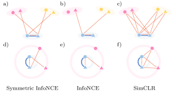
Figure 3: Illustration of positive / negative pairs of the proposed and baseline methods. From a) to f), the colors (blue, magenta, and yellow) mean different cluster labels. The light-colored manifolds in a) and d) express true clusters. In a) (reps. d)), the set of clusters composes Three-Blobs (resp. Two-Rings). A pair of the small circle and triangle symbols with the same color means a pair of a data point $x$ and the transformed data point $t(x)$ (i.e., so-called positive pair). The two data points connected by the red dash line (resp. blue straight or curved line) are enforced to be distant (resp. close) to each other. Especially in a) and d), the effect expressed by the red dash lines (resp. blue straight or curved line) are brought by making $\ell_{\rm ng}(x_{i})$ (resp. $\ell_{\rm ps}(x_{i})$) of Eq.(20) to be small. In b) and e), the effect expressed by the red dash lines (resp. blue straight or curved line) are brought by making $\ell^{\prime}_{\rm ng}(x_{i})$ (resp. $\ell^{\prime}_{\rm ps}(x_{i})$) of Eq.(21) to be small. In c) and f), the effect expressed by the red dash lines (resp. blue straight or curved line) are brought by making $\ell^{\prime\prime}_{\rm ng}(x_{i})$ (resp. $\ell^{\prime\prime}_{\rm ps}(x_{i})$) of Eq.(22) to be small.

Suppose that values of the point-wise contrastive losses are small enough. In this case, we can see the difference on stability between $-(\hat{I}_{\text{nce}}+\hat{I}^{\prime}_{\text{nce}})/2$ and $-\hat{I}_{\text{nce},q}$ by comparing a) vs. b) and d) vs. e) in Figure 3. In this figure, it is observed that the empirical symmetric InfoNCE produces more stable contrastive effects than the empirical InfoNCE.

We also compare $-(\hat{I}_{\text{nce}}+\hat{I}^{\prime}_{\text{nce}})/2$ and the loss of SimCLR introduced in Chen et al., (2020). To do so, consider the loss of SimCLR defined by a mini-batch $\mathcal{B}$. Let $L^{\mathcal{B}}_{\rm SimCLR}$ denote the loss of SimCLR with the mini-batch $\mathcal{B}$. Then, let $\ell^{\prime\prime}_{\rm ps}(x_{i})$ and $\ell^{\prime\prime}_{\rm ng}(x_{i})$ ($x_{i}\in\mathcal{B}$) denote the point-wise positive loss and point-wise negative loss by,

$$L^{\mathcal{B}}_{\rm SimCLR}=\frac{1}{|\mathcal{B}|}\sum_{x_{i}\in\mathcal{B}}\ell^{\prime\prime}_{\rm ps}(x_{i})+\ell^{\prime\prime}_{\rm ng}(x_{i}).$$ (22)

In this case, we can see the difference via a) vs. c) and d) vs. f) in Figure 3. Since the symmetric InfoNCE produces similar contrastive effects to SimCLR does, the symmetric InfoNCE is interpreted as a simplified variant of SimCLR. We however note that it is not easy to theoretically analyze SimCLR unlike our symmetric InfoNCE, since $L^{\mathcal{B}}_{\rm SimCLR}$ is designed based on heuristics.

Appendix D Details of MIST

D.1 Details of MIST Objective

To understand Eq.(11), let us see an effect brought by minimization of each term ($R_{\rm vat}$, $-H(Y)$, $H(Y|X)$, $L_{\rm ps}$, and $L_{\rm ng}$) via Figure 4. In this figure, the left pictures a) and c) show true clusters defined by the set of data points in the original space $\mathbb{R}^{d}$. Each color expresses a distinct true label. The pictures b) and d) show what kind of effects is brought by minimization of each term in the representation space $\mathbb{R}^{C}$. We here suppose that the appropriate hyper-parameters are used for Eq.(11). In both b) and d), minimization of $R_{\rm vat}$ makes the model $g_{\theta}$ acquire the local smoothness; see Eq.(12). In addition, minimization of $L_{\rm ps}$ makes the model predict the same cluster labels for the topologically close two data points. Note that, while minimization of $L_{\rm ps}$ defined by $\mathcal{T}_{\mathfrak{e}}$ in Definition 3 brings the similar effect (see b) in Figure 4) to the effect of $R_{\rm vat}$, minimization of $L_{\rm ps}$ defined by $\mathcal{T}_{\mathfrak{g}}$ in Definition 4 brings clearly different effect from $R_{\rm vat}$. For understanding this clear difference, observe that $x_{i}$ and $t_{i}(x_{i})$ in d) are forced to be close via minimization of $L_{\rm ps}$. Minimization of $-H(Y)$ (i.e., forcing $p_{\theta}(y)\in\Delta^{C-1}$ to be uniform) makes the model return the non-degenerate clustering result. Moreover, minimization of $H(Y|X)$ makes the model return a one-hot vector. Thus, it assists each cluster to be distant. At last, as discussed at Section 3.3, minimization of $L_{\rm ng}$ also makes the model return the non-degenerate clustering result.

Algorithm 1 : MIST

1:Input Unlabeled dataset: $\mathcal{D}=\{x_{i}\}_{i=1}^{n}$. Model of $p(y|x)$: $g_{\theta}(x)$. Hyper-parameters: $\mu,\gamma,\eta>0$. Generative process: $\mathcal{T}$ with a conditional probability $p(t|x)$, where $x\in\mathbb{R}^{d}$ and $t:\mathbb{R}^{d}\to\mathbb{R}^{d}$. If $\mathcal{D}$ is complex dataset, employ $\mathcal{T}_{\mathfrak{g}}$ of Definition 4. Otherwise, employ $\mathcal{T}_{\mathfrak{e}}$ of Definition 3. Mini-batch size $m$. Number of epochs: $n_{\rm ep}$.

2:Output Set of estimated cluster labels with $\mathcal{D}$: $\{\hat{y}_{i}\}_{i=1}^{n}$.

3:Initialize the trainable parameter $\theta$.

4:for $epoch=1,\cdots,n_{\rm ep}$ do

5:     for $l=0,1,\cdots,\lfloor\frac{n}{m}\rfloor$ do

6:         Randomly pick up $x_{i_{1}},\cdots,x_{i_{m}}\in\mathcal{D}$.

7:         

Compute $x_{i_{k}}^{\prime}=t_{i_{k}}(x_{i_{k}}),i=1,\cdots,m$, where $t_{i_{k}}\sim p(t|x_{i_{k}})$, and $p(t|x_{i_{k}})$ is defined via either $\mathcal{T}_{\mathfrak{e}}$ or $\mathcal{T}_{\mathfrak{g}}$.

8:         

Update the parameter $\theta$ by the SGD for the loss function in Eq.(11) computed using the mini-batch $\mathcal{B}=\{x_{i_{k}}\}_{k=1}^{m}$ and $\{x_{i_{k}}^{\prime}\}_{k=1}^{m}$.

     

9:Let $\theta^{*}$ be the estimated parameter.

10:$\hat{y}_{i}=\arg\max_{y\in\{1,\cdots,C\}}g_{\theta^{\ast}}^{y}(x_{i})$ for $i=1,\cdots,n$.

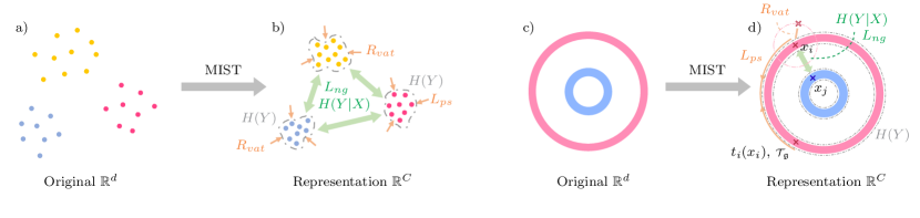
Figure 4: Intuitive illustration of MIST. Effect of each term in Eq.(11) is displayed for Three-Blobs and Two-Rings. In a) and c), the true clusters in the original space are shown, where colors mean cluster labels. In b) and d), effect of each term in Eq.(11) in the representation space is shown.

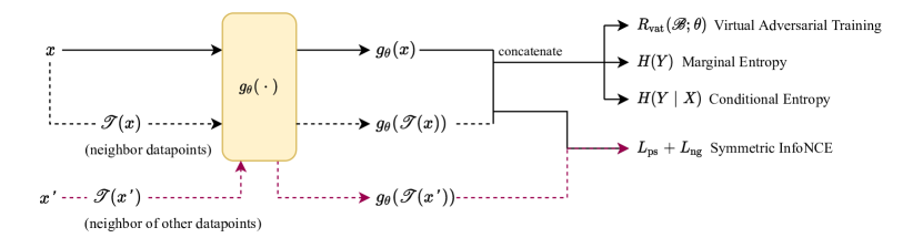
Figure 5: MIST architecture.

As recently proposed methods that are similar to MIST, we list Van Gansbeke et al., (2020); Li et al., (2021); Dang et al., (2021). The above three methods focus on the image domain (i.e., Scenario1 of Section 1.2). In the above three methods, either InfoNCE or SimCLR is employed to enhance the clustering performance. Moreover, the scenario these related works focus on is different from Scenario2. Furthermore, all the three studies do not provide any theoretical analysis of their proposed methods.

D.2 Time and Memory Complexities with $\mathcal{T}_{\mathfrak{e}}$ and $\mathcal{T}_{\mathfrak{g}}$

Suppose that we construct the non-approximated K-NN graph on $\mathcal{D}$ by using Euclidean distance. Then, the time complexity with $\mathcal{T}_{\mathfrak{e}}$ is $O(dn^{2})$, where $d$ is the dimension of a feature vector. The memory complexity is $O(K_{0}n)$. As for $\mathcal{T}_{\mathfrak{g}}$, time and memory complexities are $O\left((K_{0}+\log n)n^{2}\right)$ and $O(n^{2})$, respectively (Moscovich et al.,, 2017). Note that if we construct the approximated K-NN graph on $\mathcal{D}$ by the Euclidean distance, the time complexity with $\mathcal{T}_{\mathfrak{e}}$ is reduced to $O(dn\log n)$ (Wang et al.,, 2013; Zhang et al.,, 2013).

Appendix E Experiment Details

E.1 Details of Datasets

We used Two-Moons and Two-Rings in scikit-learn. For the former dataset, we set $0.05$ as the noise parameter. For the latter dataset we set $0.01$ and $0.35$ as noise and factor parameters respectively. For SVHN, STL, CIFAR10, CIFAR100, Omniglot and Reuters10K, we used the datasets on GitHub. As for MNIST and 20news, Keras (Géron,, 2019) was used. The summary of all the datasets is shown in Table 7. In the following, we review how features of the eight real-world datasets are obtained.

Table 7: Summary of the ten datasets used in our experiments.

	#Points	#Cluster	Dimension	%Largest Cluster	%Smallest Cluster
Two-Moons	5000	2	2	50%	50%
Two-Rings	5000	2	2	50%	50%
MNIST	70000	10	784	11%	9%
SVHN	99289	10	960	19%	6%
STL	13000	10	2048	10%	10%
CIFAR10	60000	10	2048	10%	10%
CIFAR100	60000	100	2048	1%	1%
Omniglot	40000	100	441	1%	1%
20news	18040	20	2000	5%	3%
Reuters10K	10000	4	2000	43%	8%

• MNIST: It is a hand-written digits classification dataset with $28\times 28$ single-channel images. The value of each pixel is linearly normalized into $\left[0,1\right]$ and then flattened to a $784$ dimensional feature vector.

• STL: It is a labelled subset of ImageNet (Jia Deng et al.,, 2009) with $96\times 96$ colored images. We adopted features from Hu et al., (2017), which is extracted by pre-trained 50-layer ResNets.

• CIFAR10: It is a dataset with ten clusters, $32\times 32$ colored images. We adopted features from Hu et al., (2017), which is extracted by pre-trained 50-layer ResNets.

• CIFAR100: It is a dataset with one hundred clusters, $32\times 32$ colored images. We adopted features from Hu et al., (2017), which is extracted by pretrained 50-layer ResNets.

• Omniglot: It is a hand-written character recognition dataset. We adopted the processing results from Hu et al., (2017), which is an one hundred clusters dataset with twenty unique data points per class. Twenty times affine augmentations were applied as in Hu et al., (2017), so there are $100\times 20\times 20=40000$ images available. Images were sized $21\times 21$ single-channel, linearly normalized into $\left[0,1\right]$ and flattened into feature vectors.

• 20news: It is a dataset of news documents across twenty newsgroups. We adopted the processing code from Hu et al., (2017). It used the data from python package scikit-learn (Géron,, 2019) and processed using tf-idf features with ’english’ stopwords.

• SVHN: It is a dataset with street view house numbers. Following Hu et al., (2017), we used the features they have extracted with $960$-dimensional GIST feature (Oliva and Torralba,, 2001).

• Reuters10K: It is a dataset with English news stories. We adopted the processing results from Hu et al., (2017). It contains four categories as labels: corporate/industrial, government/social, markets and economics. ten-thousands documents were randomly sampled, and processed without stop words. tf-idf features were used as in Hu et al., (2017).

E.2 Complex and Non-Complex Topology Datasets

In order to characterize each dataset from some geometric point of view, we performed experiments with the K-means algorithm for these ten datasets; see the top row of Table 2. Here, in the K-means algorithm we use the Euclidean distance to measure how far two points are apart from each other: see Chapter 22 of Shalev-Shwartz and Ben-David, (2013) for a general objective function of the K-means algorithm. Hence, if the Top-1 accuracy with the K-means algorithm is low, then the dataset can have a complex structure so that the K-means algorithm fails to group the data points into meaningful clusters. Utilizing the results with K-means algorithm (see the second row of Table 2), we define (non-)complex topology of a dataset as follows: 1) we say a dataset has non-complex topology if the Top-1 accuracy (% According to these definitions, we classify the ten datasets into two categories; two synthetic datasets, Two-Moons and Two-Rings, are of complex topology, and the others are of non-complex topology.

Note that, strictly speaking, it is difficult to provide a rigorous definition of (non-)complex topology for a real-world dataset. Instead, we state a definition inspired by our empirical observations with the K-means algorithm for the ten different datasets.

E.3 Implementation Details with Compared Methods

• K-means: sklearn.cluster.KMeans from scikit-learn.

• SC: sklearn.cluster.SpectralClustering from scikit-learn with 50 - ’nearest neighbors’ Graph and ’amg’ eigen solver.

• GMMC: sklearn.mixture.GaussianMixture from scikit-learn with diagonal covariance matrices.

• DEC: Keras implementation of Xie et al., (2016) is used.

• SpectralNet: We used the version at commit ce99307 with tensorflow 1.15, keras 2.1.6, Ubuntu 18.04 since we found that this is the only configuration that reproduces paper result in our environments. For real-world datasets, we used the 10-dimensional VaDE representation obtained in this work (see implementation details of VaDE) as input to SpectralNet. 10 neighbors were used with approximated nearest neighbor search. For Toy-sets, we have used the raw 2-dimensional input with official hyper-parameter setups for ”CC” dataset in SpectralNet.

• VaDE: We added the constraint that Gaussian Mixture component weight $\pi>0$ to avoid numerical instabilities. We did not use the provided pretraining weights since we cannot reproduce the pretraining process for all datasets.

• IMSAT: Given an unlabeled dataset $\mathcal{D}$ and the number of clusters, we train a clustering model of IMSAT by using $\mathcal{D}$ via Eq.(15). In addition, we define the adaptive radius $\epsilon_{i}$ in VAT as same with one defined in MIST: see also Appendix E.5. Moreover, for synthetic datasets, we set $(0.1,0.5)$ to $(\lambda_{1},\lambda_{2})$ of Eq.(15), and set $0.1$ to $\xi$ in VAT. For real-world datasets, we set $(0.1,4)$ to $(\lambda_{1},\lambda_{2})$ of Eq.(15), and set $10$ to $\xi$ in VAT.

• IIC: Since we consider Scenario2, we cannot define the transformation function via the domain-specific knowledge. Therefore, we define it via $\mathcal{T}_{\mathfrak{e}}$ of Definition 3 for all ten datasets as follows. For the synthetic datasets and the image datasets, $K_{0}=10$ is used. For the text datasets, $K_{0}=100$ is used. The above values of $K_{0}$ are selected by the hyper-parameter tuning.

• CatGAN: We adopted the implementation from here and moved it to GPU. Since the original CatGAN experiments have used CNNs and cannot be applied to general-purpose datasets, we substituted CNNs in both generator and discriminator with a 4-layer MLP.

• SELA: We used the official implementation with single head and known cluster numbers. We replaced the Convolutional Network in the original work by a simple MLP identical to our MIST implementation as we focusing on general purpose unsupervised learning instead of images. We also disabled data-augmentation steps presented in the original work of SELA.

• SCAN: We adopted the loss computation part from official implementation and used MIST’s framework to implement SCAN. Since we focus on generic datasets without specific domain knowledge, data augmentations are removed and SCAN learns solely on nearest neighbors. Same input data (and feature extraction steps) as MIST are used for our SCAN implementation.

E.4 Two-Dimensional Visualization

Panels a)$\sim$h) in Figure 1 were obtained by the following procedure. For two-dimensional visualization with real-world datasets, we employ UMAP (McInnes et al.,, 2018), and implement it using the public code, where we set ten and two to ”n$\_$neighbors” and ”n$\_$components”. In addition, we fix the above two parameters with UMAP for all visualization of real-world datasets.

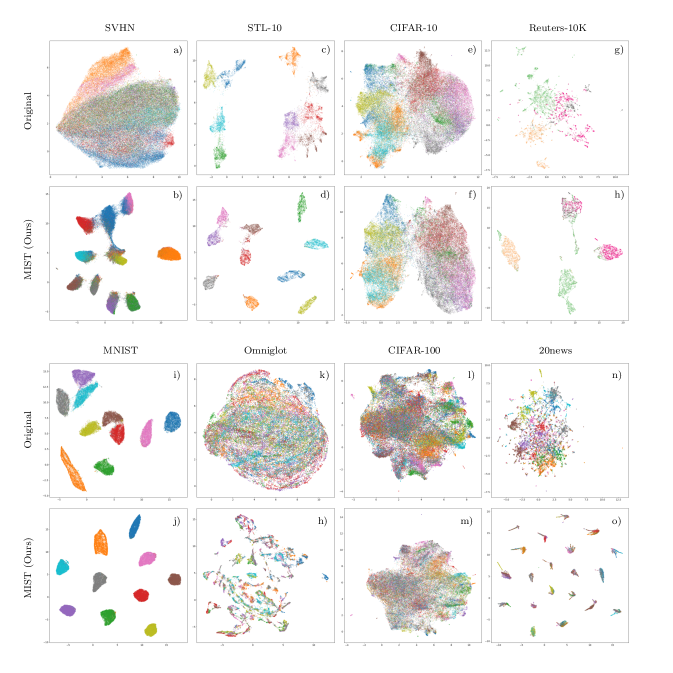
Figure 6: Two-dimensional visualizations of original datasets and their representations by MIST. Visualization of a original dataset is obtained via the same manner with panel a) of Figure 1, while that of MIST representation is obtained via the same manner with panel g) of Figure 1.

• a): Input MNIST dataset $\mathcal{D}_{\rm mnist}=\{x_{i}\}_{i=1}^{n}$, where $x_{i}\in\mathbb{R}^{784}$ and $n=70000$, to UMAP. Then, we obtain the two-dimensional vectors of $\mathcal{D}_{\rm mnist}$. Then, assign true labels to the vectors.

• c): Firstly, using $\mathcal{D}_{\rm mnist}$, train IMSAT of Eq.(15) where $(\lambda_{1},\lambda_{2})=(0.1,4)$. Moreover, for VAT in IMSAT, we set ten to $\xi$, and define the adaptive radius $\epsilon_{i}$ as same with one defined in MIST; see also Appendix E.5. Input $\mathcal{D}_{\rm mnist}$ to the trained clustering model whose last layer (a softmax function) is removed. Then, get the output whose dimension is $C=10$. Thereafter, we feed the output to UMAP, and we obtain the two-dimensional vectors. Thereafter, assign true labels to the vectors.

• e): Firstly, using $\mathcal{D}_{\rm mnist}$, train a clustering MLP of SpectralNet. SpectralNet’s official hyper-parameter setups are used. Input $\mathcal{D}_{\rm mnist}$ to the trained clustering model whose last layer (a softmax function) is removed. Then, get the output whose dimension is $C=10$. Thereafter, we feed the output to UMAP, and we obtain the two-dimensional vectors. Thereafter, assign true labels to the vectors.

• g): Firstly, using $\mathcal{D}_{\rm mnist}$, train clustering neural network model with MIST whose hyper-parameters are defined in Appendix E.5. Input $\mathcal{D}_{\rm mnist}$ to the trained clustering model whose last layer defined by the softmax is removed, and get the output. Then, we input the output to UMAP, and we obtain the two-dimensional vectors. Thereafter, assign true labels to the vectors.

• b), d), f), h): Since a data point in Two-Rings dataset $\mathcal{D}_{\rm two\_rings}$ already belongs to two-dimensional space, we just visualize the data point location with its label information in the panel b). With detail of $\mathcal{D}_{\rm two\_rings}$, see Appendix E.1. For the panels d), f) and h), we firstly predict the cluster labels by using corresponding clustering method. Then, visualize the data point location with its predicted cluster label.

In Figure 6, we additionally show two-dimensional visualization results of all eight real-world datasets. In this figure, visualizations of the first row were obtained by the same manner with the panel a) of Figure 1. Visualizations (by MIST) of the second row in Figure 6 were obtained by the same manner with the panel g) of Figure 1.

E.5 Hyper-Parameter Tuning

Table 8: All hyper-parameters related to MIST of Algorithm 1. In the first (resp. second) column, the hyper-parameters (resp. reference) are shown.

Hyper-Parameters	Reference
$(\mu,\eta,\gamma)$	MIST objective of Eq.(11)
$(\alpha,\tau)$	Critic function of Eq.(3)
$(K_{0},\beta)$	Definition 3 and 4
$(\xi,\epsilon_{i})$	VAT of Eq.(13)
$(m,n_{\rm ep})$	Algorithm 1

Table 8 shows all hyper-parameters related to MIST algorithm. Throughout numerical experiments of Section 4, we set $250,50$ as $m,n_{\rm ep}$, respectively. In addition, following Hu et al., (2017), we respectively fix $\epsilon_{i}$ of VAT to $\epsilon_{i}=0.25\times\left\|x_{i}-x^{(10)}_{i}\right\|_{2}$, where $x_{i}\in\mathcal{D}$ and $x^{(10)}_{i}$ is the tenth nearest neighbor data point from $x_{i}$ on $\mathcal{D}$ with the Euclidean metric. Note that for the synthetic datasets (resp. real-world datasets), the generative process $\mathcal{T}_{\mathfrak{g}}$ of Definition 4 (resp. the generative process $\mathcal{T}_{\mathfrak{e}}$ of Definition 3) is employed.

Table 9: Candidates with some hyper-parameters related in MIST and MIST with $\hat{I}_{\rm nce}$ of Table 2. The symbol of $\leftarrow$ indicates the same value to the cell in the left. Real-world & Image means MNIST, SVHN, STL, CIFAR10, CIFAR100, Omniglot. Real-world & Text means 20news and Reuters10K. Synthetic means both Two-Moons and Two-Rings.

Hyper-Parameters	Real-world & Image	Real-world & Text	Synthetic
$(\mu,\eta,\gamma)$	$\{(0.045,5,1.5),(0.045,6,1.5),$	$\leftarrow$	$\{(0.1,15,10),(0.1,15.5,10),$
	$\;\;\;(0.05,5,1.5),(0.04,6,1.5)\}$		$(0.1,16,10)\}$
$\alpha$	$\{0,1,2\}$	$\leftarrow$	$\leftarrow$
$\tau$	$\{0.01,0.05,0.1,1,10\}$	$\leftarrow$	$\leftarrow$
$(K_{0},\beta)$	$\{(5,0),(7,0),(10,0),(15,0)\}$	$\{(50j,2/3),(50j,4/5)\;|\;j\in\{1,..,4\}\}$	$\{(15,j/10)\;|\;j\in\{0,..,10\}\}$
$\xi$	$\{0.1,1,10,100\}$	$\leftarrow$	$\leftarrow$

In numerical experiments of Table 2, the other hyper-parameters are tuned within the corresponding candidates shown in Table 9. Those candidates were decided by the following procedure:

• $(\mu,\eta,\gamma)$: Since MIST is based on IMSAT, following Hu et al., (2017), for real-world datasets, we manually search efficient candidates, which safisfy the following criterion, inside the region including $\mu\eta=0.4$ and $\mu=0.1$: candidates which work well for MIST and MIST with $\hat{I}_{\rm nce}$ of Table 2. Note that, in IMSAT objective of Eq.(15), the authors set $\mu=0.1$ and $\eta=4$ in their official code. For the synthetic datasets, the candidates were decided via totally manual searching.

• $(\alpha,\tau)$ and $(K_{0},\beta)$: We essentially conducted manual searching for candidates, which can be efficient for both MIST and MIST with $\hat{I}_{\rm nce}$. When we select the candidates of $K_{0}$, we follow the same strategy of Shaham et al., (2018).

• $\xi$: We chose values that are around ten, since ten is set as $\xi$ in the official IMSAT code.

As for criterion of hyper-parameter tuning of the MIST and MIST with $\hat{I}_{\rm nce}$, we employed the following: for each (either real-world or synthetic), the most efficient $(\mu,\eta,\gamma,\alpha,\tau,\xi)$ should be found, while $(K_{0},\beta)$ can be adaptive for ten datasets. To find the best efficient one, we used a tuning method described in Appendix G of Hu et al., (2017), where a set of hyper-parameters, that can have the highest average clustering accuracy over several datasets, are selected. The tuning result of the MIST is shown in Table 10.

Table 10: Selected hyper-parameters with MIST of Table 2. The symbol of $\leftarrow$ indicates the same value to the cell in the left.

	MNIST, SVHN, STL, CIFAR100, Omniglot	CIFAR10	20news	Reuters10K	Two-Moons	Two-Rings
$(\mu,\eta,\gamma)$	$(0.045,5,1.5)$	$\leftarrow$	$\leftarrow$	$\leftarrow$	$(0.1,15.5,10)$	$\leftarrow$
$(\alpha,\tau)$	$(1,0.05)$	$\leftarrow$	$\leftarrow$	$\leftarrow$	$\leftarrow$	$\leftarrow$
$(K_{0},\beta)$	$(7,0)$	$(15,0)$	$(200,4/5)$	$(50,4/5)$	$(15,0)$	$(15,0.6)$
$\xi$	10	$\leftarrow$	$\leftarrow$	$\leftarrow$	0.1	$\leftarrow$

Moreover, for all combinations except for (\scriptsize{\lower0.2ex\hbox{B}}⃝, \scriptsize{\lower0.2ex\hbox{C}}⃝) in Table 3, we at first manually selected the candidates of hyper-parameters. Then, for each combination, we conducted hyper-parameter tuning, whose criterion is same with one employed for tuning hyper-parameters in MIST of Table 2. The tuning results are shown in Table 11.

Table 11: Selected value for each hyper-parameter with experiments related to Table 3. From the second to sixth columns, hyper-parameter values selected for real-world datasets are shown. The symbol of ”$-$” means that the hyper-parameter is not needed. The symbol of $\leftarrow$ indicates the same value to the cell in the left. In the last column, hyper-parameter values to define six combinations are shown. As for $(\alpha,K_{0},\beta,\xi)$, the same values shown in Table 10 are employed.

	(\scriptsize{\lower0.2ex\hbox{D}}⃝)	(\scriptsize{\lower0.2ex\hbox{B}}⃝, \scriptsize{\lower0.2ex\hbox{D}}⃝)	(\scriptsize{\lower0.2ex\hbox{A}}⃝, \scriptsize{\lower0.2ex\hbox{D}}⃝)	(\scriptsize{\lower0.2ex\hbox{B}}⃝, \scriptsize{\lower0.2ex\hbox{C}}⃝, \scriptsize{\lower0.2ex\hbox{D}}⃝)	(\scriptsize{\lower0.2ex\hbox{A}}⃝, \scriptsize{\lower0.2ex\hbox{B}}⃝, \scriptsize{\lower0.2ex\hbox{C}}⃝)	Two-Rings
$\mu$	$-$	$\leftarrow$	0.045	$-$	0.1	0.1
$\eta$	$-$	1	$-$	1	4	15.5
$\gamma$	$-$	10	1.5	10	$-$	10
$\tau$	1.0	$\leftarrow$	$\leftarrow$	0.1	$-$	1.0

References

- Amari and Ohara, (2011) Amari, S. I. and Ohara, A. (2011). Geometry of q-exponential family of probability distributions. Entropy, 13(6):1170–1185.
- Asano et al., (2019) Asano, Y. M., Rupprecht, C., and Vedaldi, A. (2019). Self-labelling via simultaneous clustering and representation learning. In International Conference on Learning Representations.
- Avgerinos et al., (2020) Avgerinos, C., Solachidis, V., Vretos, N., and Daras, P. (2020). Non-Parametric Clustering Using Deep Neural Networks. IEEE Access, 8:153630–153640.
- Bai et al., (2021) Bai, S., Zheng, Z., Wang, X., Lin, J., Zhang, Z., Zhou, C., Yang, H., and Yang, Y. (2021). Connecting language and vision for natural language-based vehicle retrieval. In Proceedings of the IEEE/CVF Conference on Computer Vision and Pattern Recognition, pages 4034–4043.
- Bartlett and Mendelson, (2002) Bartlett, P. L. and Mendelson, S. (2002). Rademacher and Gaussian complexities: Risk bounds and structural results. Journal of Machine Learning Research, 3(Nov):463–482.
- Belghazi et al., (2018) Belghazi, M. I., Baratin, A., Rajeshwar, S., Ozair, S., Bengio, Y., Courville, A., and Hjelm, D. (2018). Mutual information neural estimation. In Proceedings of the 35th International Conference on Machine Learning, volume 80 of Proceedings of Machine Learning Research, pages 531–540. PMLR.
- Bengio et al., (2013) Bengio, Y., Courville, A., and Vincent, P. (2013). Representation learning: A review and new perspectives. IEEE Transactions on Pattern Analysis and Machine Intelligence, 35(8):1798–1828.
- Budimir et al., (2000) Budimir, I., Dragomir, S. S., and Pecaric, J. (2000). Further reverse results for jensen’s discrete inequality and applications in information theory. RGMIA research report collection, 3(1).
- Caron et al., (2018) Caron, M., Bojanowski, P., Joulin, A., and Douze, M. (2018). Deep clustering for unsupervised learning of visual features. In Proceedings of the European Conference on Computer Vision (ECCV).
- Caron et al., (2020) Caron, M., Misra, I., Mairal, J., Goyal, P., Bojanowski, P., and Joulin, A. (2020). Unsupervised learning of visual features by contrasting cluster assignments. In Advances in Neural Information Processing Systems, pages 9912–9924.
- Chapelle et al., (2006) Chapelle, O., Schölkopf, B., and Zien, A., editors (2006). Semi-Supervised Learning. The MIT Press.
- Chen, (2015) Chen, G. (2015). Deep learning with nonparametric clustering. arXiv preprint arXiv:1501.03084.
- Chen et al., (2020) Chen, T., Kornblith, S., Norouzi, M., and Hinton, G. (2020). A simple framework for contrastive learning of visual representations. In Proceedings of the 37th International Conference on Machine Learning, volume 119 of Proceedings of Machine Learning Research, pages 1597–1607. PMLR.
- Coates et al., (2011) Coates, A., Ng, A., and Lee, H. (2011). An analysis of single-layer networks in unsupervised feature learning. In Proceedings of the Fourteenth International Conference on Artificial Intelligence and Statistics, volume 15 of Proceedings of Machine Learning Research, pages 215–223. PMLR.
- Cover, (1999) Cover, T. M. (1999). Elements of information theory. John Wiley & Sons.
- Dang et al., (2021) Dang, Z., Deng, C., Yang, X., Wei, K., and Huang, H. (2021). Nearest neighbor matching for deep clustering. In Proceedings of the IEEE Computer Society Conference on Computer Vision and Pattern Recognition, pages 13688–13697.
- Day, (1969) Day, N. E. (1969). Estimating the components of a mixture of normal distributions. Biometrika, 56(3):463.
- Ester et al., (1996) Ester, M., Kriegel, H.-P., Sander, J., and Xu, X. (1996). A density-based algorithm for discovering clusters in large spatial databases with noise. In Proceedings of the 2nd International Conference on Knowledge Discovery and Data Mining, volume 96, pages 226–231.
- Géron, (2019) Géron, A. (2019). Hands-on machine learning with Scikit-Learn, Keras and TensorFlow: concepts, tools, and techniques to build intelligent systems. O’Reilly Media.
- Girolami, (2002) Girolami, M. (2002). Mercer kernel-based clustering in feature space. IEEE Transactions on Neural Networks, 13(3):780–784.
- Grill et al., (2020) Grill, J. B., Strub, F., Altché, F., Tallec, C., Richemond, P. H., Buchatskaya, E., Doersch, C., Pires, B. A., Guo, Z. D., Azar, M. G., Piot, B., Kavukcuoglu, K., Munos, R., and Valko, M. (2020). Bootstrap your own latent a new approach to self-supervised learning. Advances in Neural Information Processing Systems, 2020-December:21271–21284.
- Guo et al., (2017) Guo, X., Gao, L., Liu, X., and Yin, J. (2017). Improved deep embedded clustering with local structure preservation. In IJCAI International Joint Conference on Artificial Intelligence, pages 1753–1759.
- Gupta et al., (2020) Gupta, D., Ramjee, R., Kwatra, N., and Sivathanu, M. (2020). Unsupervised Clustering using Pseudo-semi-supervised Learning. In International Conference on Learning Representations.
- He et al., (2015) He, K., Zhang, X., Ren, S., and Sun, J. (2015). Delving deep into rectifiers: Surpassing human-level performance on imagenet classification. In Proceedings of the IEEE International Conference on Computer Vision, volume 2015 International Conference on Computer Vision, ICCV 2015, pages 1026–1034.
- He et al., (2016) He, K., Zhang, X., Ren, S., and Sun, J. (2016). Deep residual learning for image recognition. In Proceedings of the IEEE Computer Society Conference on Computer Vision and Pattern Recognition, pages 770–778.
- Hinton et al., (2012) Hinton, G. E., Srivastava, N., Krizhevsky, A., Sutskever, I., and Salakhutdinov, R. R. (2012). Improving neural networks by preventing co-adaptation of feature detectors. arXiv preprint arXiv:1207.0580.
- Hu et al., (2017) Hu, W., Miyato, T., Tokui, S., Matsumoto, E., and Sugiyama, M. (2017). Learning discrete representations via information maximizing self-augmented training. In Proceedings of the 34th International Conference on Machine Learning, volume 70 of Proceedings of Machine Learning Research, pages 1558–1567. PMLR.
- Ioffe and Szegedy, (2015) Ioffe, S. and Szegedy, C. (2015). Batch normalization: Accelerating deep network training by reducing internal covariate shift. In 32nd International Conference on Machine Learning, ICML 2015, volume 1, pages 448–456. PMLR.
- Ji et al., (2019) Ji, X., Vedaldi, A., and Henriques, J. (2019). Invariant information clustering for unsupervised image classification and segmentation. In Proceedings of the IEEE International Conference on Computer Vision, pages 9864–9873.
- Jia Deng et al., (2009) Jia Deng, Wei Dong, Socher, R., Li-Jia Li, Kai Li, and Li Fei-Fei (2009). ImageNet: A large-scale hierarchical image database. In 2009 IEEE Conference on Computer Vision and Pattern Recognition, pages 248–255. Ieee.
- Jiang et al., (2017) Jiang, Z., Zheng, Y., Tan, H., Tang, B., and Zhou, H. (2017). Variational deep embedding: An unsupervised generative approach to Clustering. In IJCAI International Joint Conference on Artificial Intelligence, pages 1965–1972.
- Ketkar and Moolayil, (2017) Ketkar, N. and Moolayil, J. (2017). Introduction to PyTorch. In Deep Learning with Python, pages 195–208. Springer.
- Kingma and Ba, (2015) Kingma, D. P. and Ba, J. L. (2015). Adam: A method for stochastic optimization. In 3rd International Conference on Learning Representations, ICLR 2015 - Conference Track Proceedings.
- Kuhn, (1955) Kuhn, H. W. (1955). The Hungarian method for the assignment problem. Naval research logistics quarterly, 2(1-2):83–97.
- Lake et al., (2011) Lake, B. M., Salakhutdinov, R., Gross, J., and Tenenbaum, J. B. (2011). One shot learning of simple visual concepts. In In Proceedings of the 33rd Annual Conference of the Cognitive Science Society, volume 33.
- Lang, (1995) Lang, K. (1995). NewsWeeder: Learning to filter netnews. In Machine Learning Proceedings 1995, pages 331–339. Elsevier.
- Lecun et al., (2015) Lecun, Y., Bengio, Y., and Hinton, G. (2015). Deep learning. Nature, 521(7553):436–444.
- LeCun et al., (1989) LeCun, Y., Boser, B., Denker, J. S., Henderson, D., Howard, R. E., Hubbard, W., and Jackel, L. D. (1989). Backpropagation applied to handwritten zip code recognition. Neural Computation, 1(4):541–551.
- LeCun et al., (1998) LeCun, Y., Bottou, L., Bengio, Y., and Haffner, P. (1998). Gradient-based learning applied to document recognition. Proceedings of the IEEE, 86(11):2278–2323.
- Lewis et al., (2004) Lewis, D. D., Yang, Y., Rose, T. G., and Li, F. (2004). RCV1: A new benchmark collection for text categorization research. Journal of Machine Learning Research, 5(Apr):361–397.
- Li et al., (2021) Li, Y., Hu, P., Liu, Z., Peng, D., Zhou, J. T., and Peng, X. (2021). Contrastive clustering. In Proceedings of the AAAI Conference on Artificial Intelligence, volume 35, pages 8547–8555.
- Liao and Berg, (2019) Liao, J. G. and Berg, A. (2019). Sharpening Jensen’s inequality. The American Statistician, 73(3).
- MacQueen, (1967) MacQueen, J. (1967). Some methods for classification and analysis of multivariate observations. In Proceedings of the fifth Berkeley symposium on mathematical statistics and probability, volume 1, pages 281–297. Oakland, CA, USA.
- Matsuzoe and Ohara, (2012) Matsuzoe, H. and Ohara, A. (2012). Geometry for q-exponential families. In Recent progress in differential geometry and its related fields, pages 55–71. World Scientific.
- Mautz et al., (2019) Mautz, D., Plant, C., and Böhm, C. (2019). Deep embedded cluster tree. In 2019 IEEE International Conference on Data Mining (ICDM), pages 1258–1263.
- McConville et al., (2020) McConville, R., Santos-Rodríguez, R., Piechocki, R. J., and Craddock, I. (2020). N2D: (not too) deep clustering via clustering the local manifold of an autoencoded embedding. In Proceedings - International Conference on Pattern Recognition, pages 5145–5152.
- McInnes et al., (2018) McInnes, L., Healy, J., Saul, N., and Großberger, L. (2018). UMAP: Uniform manifold approximation and projection. Journal of Open Source Software, 3(29):861.
- Miyato et al., (2019) Miyato, T., Maeda, S. I., Koyama, M., and Ishii, S. (2019). Virtual adversarial training: A regularization method for supervised and semi-supervised learning. IEEE Transactions on Pattern Analysis and Machine Intelligence, 41(8):1979–1993.
- Mohri et al., (2018) Mohri, M., Rostamizadeh, A., and Talwalkar, A. (2018). Foundations of machine learning. MIT press.
- Monnier et al., (2020) Monnier, T., Groueix, T., and Aubry, M. (2020). Deep transformation-invariant clustering. Advances in Neural Information Processing Systems, 33:7945–7955.
- Moscovich et al., (2017) Moscovich, A., Jaffe, A., and Nadler, B. (2017). Minimax-optimal semi-supervised regression on unknown manifolds. In Proceedings of the 20th International Conference on Artificial Intelligence and Statistics, AISTATS 2017, pages 933–942. PMLR.
- Mukherjee et al., (2019) Mukherjee, S., Asnani, H., Lin, E., and Kannan, S. (2019). ClusterGAN: Latent space clustering in generative adversarial networks. In 33rd AAAI Conference on Artificial Intelligence, AAAI 2019, pages 4610–4617.
- Nair and Hinton, (2010) Nair, V. and Hinton, G. E. (2010). Rectified linear units improve Restricted Boltzmann machines. In ICML 2010 - Proceedings, 27th International Conference on Machine Learning.
- Naudts, (2009) Naudts, J. (2009). The q-exponential family in statistical physics. Central European Journal of Physics, 7(3):405–413.
- Nazi et al., (2019) Nazi, A., Hang, W., Goldie, A., Ravi, S., and Mirhoseini, A. (2019). Generalized clustering by learning to optimize expected normalized cuts. arXiv preprint arXiv:1910.07623.
- Netzer et al., (2011) Netzer, Y., Wang, T., Coates, A., Bissacco, A., Wu, B., and Ng, A. Y. (2011). Reading digits in natural images with unsupervised feature learning. In NIPS Workshop on Deep Learning and Unsupervised Feature Learning 2011.
- Ng et al., (2002) Ng, A. Y., Jordan, M. I., and Weiss, Y. (2002). On spectral clustering: Analysis and an algorithm. Advances in Neural Information Processing Systems, 14:849–856.
- Oliva and Torralba, (2001) Oliva, A. and Torralba, A. (2001). Modeling the shape of the scene: A holistic representation of the spatial envelope. International Journal of Computer Vision, 42(3):145–175.
- Poole et al., (2019) Poole, B., Ozair, S., Van Den Oord, A., Alemi, A., and Tucker, G. (2019). On variational bounds of mutual information. In Proceedings of the 36th International Conference on Machine Learning, volume 97 of Proceedings of Machine Learning Research, pages 5171–5180. PMLR.
- Schwarz, (1978) Schwarz, G. (1978). Estimating the dimension of a model. The Annals of Statistics, 6(2):461–464.
- Shaham et al., (2018) Shaham, U., Stanton, K., Li, H., Nadler, B., Basri, R., and Kluger, Y. (2018). SpectralNet: Spectral clustering using deep neural networks. In 6th International Conference on Learning Representations.
- Shalev-Shwartz and Ben-David, (2013) Shalev-Shwartz, S. and Ben-David, S. (2013). Understanding machine learning: From theory to algorithms. Cambridge university press.
- Sibson, (1973) Sibson, R. (1973). SLINK: An optimally efficient algorithm for the single-link cluster method. The Computer Journal, 16(1):30–34.
- Sohn, (2016) Sohn, K. (2016). Improved deep metric learning with multi-class N-pair loss objective. In Advances in Neural Information Processing Systems, pages 1857–1865.
- Springenberg, (2015) Springenberg, J. T. (2015). Unsupervised and semi-supervised learning with categorical generative adversarial networks. arXiv preprint arXiv:1511.06390.
- Torralba et al., (2008) Torralba, A., Fergus, R., and Freeman, W. T. (2008). 80 million tiny images: A large data set for nonparametric object and scene recognition. IEEE Transactions on Pattern Analysis and Machine Intelligence, 30(11):1958–1970.
- Tschannen et al., (2019) Tschannen, M., Djolonga, J., Rubenstein, P. K., Gelly, S., and Lucic, M. (2019). On mutual information maximization for representation learning. In International Conference on Learning Representations.
- van den Oord et al., (2018) van den Oord, A., Li, Y., and Vinyals, O. (2018). Representation learning with contrastive predictive coding. arXiv preprint arXiv:1807.03748.
- Van Gansbeke et al., (2020) Van Gansbeke, W., Vandenhende, S., Georgoulis, S., Proesmans, M., and Van Gool, L. (2020). Scan: Learning to classify images without labels. In European Conference on Computer Vision, pages 268–285. Springer.
- Wang et al., (2013) Wang, D., Shi, L., and Cao, J. (2013). Fast algorithm for approximate k-nearest neighbor graph construction. In Proceedings - IEEE 13th International Conference on Data Mining Workshops, ICDMW 2013, pages 349–356.
- Wang et al., (2003) Wang, J., Lee, J., and Zhang, C. (2003). Kernel trick embedded Gaussian mixture model. In Algorithmic Learning Theory, pages 159–174. Springer Berlin Heidelberg.
- Wang et al., (2022) Wang, Y., Zhang, Q., Wang, Y., Yang, J., and Lin, Z. (2022). Chaos is a ladder: A new understanding of contrastive learning. In International Conference on Learning Representations.
- Xie et al., (2016) Xie, J., Girshick, R., and Farhadi, A. (2016). Unsupervised deep embedding for clustering analysis. In Proceedings of The 33rd International Conference on Machine Learning, volume 48 of Proceedings of Machine Learning Research, pages 478–487. PMLR.
- Yang et al., (2016) Yang, J., Parikh, D., and Batra, D. (2016). Joint unsupervised learning of deep representations and image clusters. In Proceedings of the IEEE Computer Society Conference on Computer Vision and Pattern Recognition, pages 5147–5156.
- Yang et al., (2020) Yang, X., Deng, C., Wei, K., Yan, J., and Liu, W. (2020). Adversarial learning for robust deep clustering. Advances in Neural Information Processing Systems, 2020-December:9098–9108.
- Zhang et al., (2013) Zhang, Y.-M., Huang, K., Geng, G., and Liu, C.-L. (2013). Fast kNN graph construction with locality sensitive hashing. In Machine Learning and Knowledge Discovery in Databases, pages 660–674. Springer Berlin Heidelberg.