Guiding Energy-based Models
via Contrastive Latent Variables

Abstract

An energy-based model (EBM) is a popular generative framework that offers both explicit density and architectural flexibility, but training them is difficult since it is often unstable and time-consuming. In recent years, various training techniques have been developed, e.g., better divergence measures or stabilization in MCMC sampling, but there often exists a large gap between EBMs and other generative frameworks like GANs in terms of generation quality. In this paper, we propose a novel and effective framework for improving EBMs via contrastive representation learning (CRL). To be specific, we consider representations learned by contrastive methods as the true underlying latent variable. This contrastive latent variable could guide EBMs to understand the data structure better, so it can improve and accelerate EBM training significantly. To enable the joint training of EBM and CRL, we also design a new class of latent-variable EBMs for learning the joint density of data and the contrastive latent variable. Our experimental results demonstrate that our scheme achieves lower FID scores, compared to prior-art EBM methods (e.g., additionally using variational autoencoders or diffusion techniques), even with significantly faster and more memory-efficient training. We also show conditional and compositional generation abilities of our latent-variable EBMs as their additional benefits, even without explicit conditional training. The code is available at https://github.com/hankook/CLEL.

1 Introduction

Generative modeling is a fundamental machine learning task for learning complex high-dimensional data distributions $p_{\text{data}}(\mathbf{x})$. Among a number of generative frameworks, energy-based models (EBMs, LeCun et al., 2006; Salakhutdinov et al., 2007), whose density is proportional to the exponential negative energy, i.e., $p_{\theta}(\mathbf{x})\propto\exp(-E_{\theta}(\mathbf{x}))$, have recently gained much attention due to their attractive properties. For example, EBMs can naturally provide the explicit (unnormalized) density, unlike generative adversarial networks (GANs, Goodfellow et al., 2014). Furthermore, they are much less restrictive in architectural designs than other explicit density models such as autoregressive (Oord et al., 2016b; a) and flow-based models (Rezende & Mohamed, 2015; Dinh et al., 2017). Hence, EBMs have found wide applications, including image inpainting (Du & Mordatch, 2019), hybrid discriminative-generative models (Grathwohl et al., 2019; Yang & Ji, 2021), protein design (Ingraham et al., 2019; Du et al., 2020b), and text generation (Deng et al., 2020).

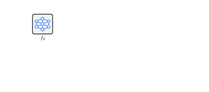
Figure 1: Illustration of the proposed Contrastive Latent-guided Energy Learning (CLEL) framework. (a) Our spherical latent-variable EBM $(f_{\theta},g_{\theta})$ learns the joint data distribution $p_{\text{data}}(\mathbf{x},\mathbf{z})$ generated by our contrastive latent encoder $h_{\phi}$. (b) The encoder $h_{\phi}$ is trained by contrastive learning with additional negative variables $\tilde{\mathbf{z}}\sim p_{\theta}(\tilde{\mathbf{z}})$. Here, $\mathbf{z}_{i}=h_{\phi}(t_{i}(\mathbf{x}))/\lVert h_{\phi}(t_{i}(\mathbf{x}))\rVert_{2}$ where $t_{i}\sim\mathcal{T}$ denotes a random augmentation, and $\mathtt{sg}(\cdot)$ denotes the stop-gradient operation.

Despite the attractive properties, training EBMs has remained challenging; e.g., it often suffers from the training instability due to the intractable sampling and the absence of the normalizing constant. Recently, various techniques have been developed for improving the training stability and the quality of generated samples, for example, gradient clipping (Du & Mordatch, 2019), short MCMC runs (Nijkamp et al., 2019), data augmentations in MCMC sampling (Du et al., 2021), and better divergence measures (Yu et al., 2020; 2021; Du et al., 2021). To further improve EBMs, there are several recent attempts to incorporate other generative models into EBM training, e.g., variational autoencoders (VAEs) (Xiao et al., 2021), flow models (Gao et al., 2020; Xie et al., 2022), or diffusion techniques (Gao et al., 2021). However, they often require a high computational cost for training such an extra generative model, or there still exists a large gap between EBMs and state-of-the-art generative frameworks like GANs (Kang et al., 2021) or score-based models (Vahdat et al., 2021).

Instead of utilizing extra expensive generative models, in this paper, we ask whether EBMs can be improved by other unsupervised techniques of low cost. To this end, we are inspired by recent advances in unsupervised representation learning literature (Chen et al., 2020; Grill et al., 2020; He et al., 2021), especially by the fact that the discriminative representations can be obtained much easier than generative modeling. Interestingly, such representations have been used to detect out-of-distribution samples (Hendrycks et al., 2019a; b), so we expect that training EBMs can benefit from good representations. In particular, we primarily focus on contrastive representation learning (Oord et al., 2018; Chen et al., 2020; He et al., 2020) since it can learn instance discriminability, which has been shown to be effective in not only representation learning, but also training GANs (Jeong & Shin, 2021; Kang et al., 2021) and out-of-distribution detection (Tack et al., 2020).

In this paper, we propose Contrastive Latent-guided Energy Learning (CLEL), a simple yet effective framework for improving EBMs via contrastive representation learning (CRL). Our CLEL consists of two components, which are illustrated in Figure 1.

• Contrastive latent encoder. Our key idea is to consider representations learned by CRL as an underlying latent variable distribution $p_{\text{data}}(\mathbf{z}|\mathbf{x})$. Specifically, we train an encoder $h_{\phi}$ via CRL, and treat the encoded representation $\mathbf{z}:=h_{\phi}(\mathbf{x})$ as the true latent variable given data $\mathbf{x}$, i.e., $\mathbf{z}\sim p_{\text{data}}(\cdot|\mathbf{x})$. This latent variable could guide EBMs to understand the underlying data structure more quickly and accelerate training since the latent variable contains semantic information of the data thanks to CRL. Here, we assume the latent variables are spherical, i.e., $\lVert\mathbf{z}\rVert_{2}=1$, since recent CRL methods (He et al., 2020; Chen et al., 2020) use the cosine distance on the latent space.

• Spherical latent-variable EBM. We introduce a new class of latent-variable EBMs $p_{\theta}(\mathbf{x},\mathbf{z})$ for modeling the joint distribution $p_{\text{data}}(\mathbf{x},\mathbf{z})$ generated by the contrastive latent encoder. Since the latent variables are spherical, we separate the output vector $f:=f_{\theta}(\mathbf{x})$ into its norm $\lVert f\rVert_{2}$ and direction $f/\lVert f\rVert_{2}$ for modeling $p_{\theta}(\mathbf{x})$ and $p_{\theta}(\mathbf{z}|\mathbf{x})$, respectively. We found that this separation technique reduces the conflict between $p_{\theta}(\mathbf{x})$ and $p_{\theta}(\mathbf{z}|\mathbf{x})$ optimizations, which makes training stable. In addition, we treat the latent variables drawn from our EBM, $\tilde{\mathbf{z}}\sim p_{\theta}(\mathbf{z})$, as additional negatives in CRL, which further improves our CLEL. Namely, CRL guides EBM and vice versa.

We demonstrate the effectiveness of the proposed framework through extensive experiments. For example, our EBM achieves 8.61 FID under unconditional CIFAR-10 generation, which is lower than those of existing EBM models. Here, we remark that utilizing CRL into our EBM training increases training time by only 10% in our experiments (e.g., 38$\rightarrow$41 GPU hours). This enables us to achieve the lower FID score even with significantly less computational resources (e.g., we use single RTX3090 GPU only) than the prior EBMs that utilize VAEs (Xiao et al., 2021) or diffusion-based recovery likelihood (Gao et al., 2021). Furthermore, even without explicit conditional training, our latent-variable EBMs naturally can provide the latent-conditional density $p_{\theta}(\mathbf{x}|\mathbf{z})$; we verify its effectiveness under various applications: out-of-distribution (OOD) detection, conditional sampling, and compositional sampling. For example, OOD detection using the conditional density shows superiority over various likelihood-based models. Finally, we remark that our idea is not limited to contrastive representation learning and we show EBMs can be also improved by other representation learning methods like BYOL (Grill et al., 2020) or MAE (He et al., 2021) (see Section 4.5).

2 Preliminaries

In this work, we mainly consider unconditional generative modeling: given a set of i.i.d. samples $\{\mathbf{x}^{(i)}\}_{i=1}^{N}$ drawn from an unknown data distribution $p_{\text{data}}(\mathbf{x})$, our goal is to learn a model distribution $p_{\theta}(\mathbf{x})$ parameterized by $\theta$ to approximate the data distribution $p_{\text{data}}(\mathbf{x})$. To this end, we parameterize $p_{\theta}(\mathbf{x})$ using energy-based models (EBMs), and incorporate contrastive representation learning (CRL) into EBMs for improving them. We briefly describe the concepts of EBMs and CRL in Section 2.1 and Section 2.2, respectively, and then introduce our framework in Section 3.

2.1 Energy-based models

An energy-based model (EBM) is a probability distribution on $\mathbb{R}^{d_{\mathbf{x}}}$, defined as follows: for $\mathbf{x}\in\mathbb{R}^{d_{\mathbf{x}}}$,

$$p_{\theta}(\mathbf{x})=\frac{\exp(-E_{\theta}(\mathbf{x}))}{Z_{\theta}},\quad\quad Z_{\theta}=\int_{\mathbb{R}^{d_{\mathbf{x}}}}\exp(-E_{\theta}(\mathbf{x}))d\mathbf{x},$$ (1)

where $E_{\theta}(\mathbf{x})$ is the energy function parameterized by $\theta$ and $Z_{\theta}$ denotes the normalizing constant, called the partition function. An important application of EBMs is to find a parameter $\theta$ such that $p_{\theta}$ is close to $p_{\text{data}}$. A popular method for finding such $\theta$ is to minimize Kullback–Leibler (KL) divergence between $p_{\text{data}}$ and $p_{\theta}$ via gradient descent:

$$D_{\text{KL}}(p_{\text{data}}\|p_{\theta}) =-\mathbb{E}_{\mathbf{x}\sim p_{\text{data}}}[\log p_{\theta}(\mathbf{x})]+\text{Constant},$$ (2)

$$\nabla_{\theta}D_{\text{KL}}(p_{\text{data}}\|p_{\theta}) =\mathbb{E}_{\mathbf{x}\sim p_{\text{data}}}[\nabla_{\theta}E_{\theta}(\mathbf{x})]-\mathbb{E}_{\tilde{\mathbf{x}}\sim p_{\theta}}[\nabla_{\theta}E_{\theta}(\tilde{\mathbf{x}})].$$ (3)

Since this gradient computation (3) is NP-hard in general (Jerrum & Sinclair, 1993), it is often approximated via Markov chain Monte Carlo (MCMC) methods. In this work, we use the stochastic gradient Langevin dynamics (SGLD, Welling & Teh, 2011), a gradient-based MCMC method for approximate sampling. Specifically, at the $(t+1)$-th iteration, SGLD updates the current sample $\tilde{\mathbf{x}}^{(t)}$ to $\tilde{\mathbf{x}}^{(t+1)}$ using the following procedure:

$$\tilde{\mathbf{x}}^{(t+1)}\leftarrow\tilde{\mathbf{x}}^{(t)}+\frac{\varepsilon^{2}}{2}\underbrace{\nabla_{\mathbf{x}}\log p_{\theta}(\tilde{\mathbf{x}}^{(t)})}_{=-\nabla_{\mathbf{x}}E_{\theta}(\tilde{\mathbf{x}}^{(t)})}+\varepsilon\bm{\delta}^{(t)},\quad\bm{\delta}^{(t)}\sim\mathcal{N}(0,I),$$ (4)

where $\varepsilon>0$ is some predefined constant, $\tilde{\mathbf{x}}^{(0)}$ denotes an initial state, and $\mathcal{N}$ denotes the multivariate normal distribution. Here, it is known that the distribution of $\tilde{\mathbf{x}}^{(T)}$ (weakly) converges to $p_{\theta}$ with small enough $\varepsilon$ and large enough $T$ under various assumptions (Vollmer et al., 2016; Raginsky et al., 2017; Xu et al., 2018; Zou et al., 2021).

Latent-variable energy-based models. EBMs can naturally incorporate a latent variable by specifying the joint density $p_{\theta}(\mathbf{x},\mathbf{z})\propto\exp(-E_{\theta}(\mathbf{x},\mathbf{z}))$ of observed data $\mathbf{x}$ and the latent variable $\mathbf{z}$. This class includes a number of EBMs: e.g., deep Boltzmann machines (Salakhutdinov & Hinton, 2009) and conjugate EBMs (Wu et al., 2021). Similar to standard EBMs, these latent-variable EBMs can be trained by minimizing KL divergence between $p_{\text{data}}(\mathbf{x})$ and $p_{\theta}(\mathbf{x})$ as described in (3):

$$\nabla_{\theta}D_{\text{KL}}(p_{\text{data}}\|p_{\theta}) =\mathbb{E}_{\mathbf{x}\sim p_{\text{data}}(\mathbf{x})}[\nabla_{\theta}E_{\theta}(\mathbf{x})]-\mathbb{E}_{\tilde{\mathbf{x}}\sim p_{\theta}(\tilde{\mathbf{x}})}[\nabla_{\theta}E_{\theta}(\tilde{\mathbf{x}})]$$ (5)

$$=\mathbb{E}_{\mathbf{x}\sim p_{\text{data}}(\mathbf{x}),\mathbf{z}\sim p_{\theta}(\mathbf{z}|\mathbf{x})}[\nabla_{\theta}E_{\theta}(\mathbf{x},\mathbf{z})]-\mathbb{E}_{\tilde{\mathbf{x}}\sim p_{\theta}(\tilde{\mathbf{x}}),\mathbf{z}\sim p_{\theta}(\mathbf{z}|\tilde{\mathbf{x}})}[\nabla_{\theta}E_{\theta}(\tilde{\mathbf{x}},\mathbf{z})],$$ (6)

where $E_{\theta}(\mathbf{x})$ is the marginal energy, i.e., $E_{\theta}(\mathbf{x})=-\log\int\exp(-E_{\theta}(\mathbf{x},\mathbf{z}))d\mathbf{z}$.

2.2 Contrastive representation learning

Generally speaking, contrastive learning aims to learn a meaningful representation by minimizing distance between similar (i.e., positive) samples, and maximizing distance between dissimilar (i.e., negative) samples on the representation space. Formally, let $h_{\phi}:\mathbb{R}^{d_{\mathbf{x}}}\rightarrow\mathbb{R}^{d_{\mathbf{z}}}$ be a $\phi$-parameterized encoder, $(\mathbf{x},\mathbf{x}_{+})$ and $(\mathbf{x},\mathbf{x}_{-})$ be positive and negative pairs, respectively. Contrastive learning then maximizes $\text{sim}(h_{\phi}(\mathbf{x}),h_{\phi}(\mathbf{x}_{+}))$ and minimizes $\text{sim}(h_{\phi}(\mathbf{x}),h_{\phi}(\mathbf{x}_{-}))$ where $\text{sim}(\cdot,\cdot)$ is a similarity metric defined on the representation space $\mathbb{R}^{d_{\mathbf{z}}}$.

Under the unsupervised setup, various methods for constructing positive and negative pairs have been proposed: e.g., data augmentations (He et al., 2020; Chen et al., 2020; Tian et al., 2020), spatial or temporal co-occurrence (Oord et al., 2018), and image channels (Tian et al., 2019). In this work, we mainly focus on a popular contrastive learning framework, SimCLR (Chen et al., 2020), which constructs positive and negative pairs via various data augmentations such as cropping and color jittering. Specifically, given a mini-batch $\mathcal{B}=\{\mathbf{x}^{(i)}\}_{i=1}^{n}$, SimCLR first constructs two augmented views $\{\mathbf{v}_{j}^{(i)}:=t_{j}^{(i)}(\mathbf{x}^{(i)})\}_{j\in\{1,2\}}$ for each data sample $\mathbf{x}^{(i)}$ via random augmentations $t_{j}^{(i)}\sim\mathcal{T}$. Then, it considers $(\mathbf{v}_{1}^{(i)},\mathbf{v}_{2}^{(i)})$ as a positive pair and $(\mathbf{v}_{1}^{(i)},\mathbf{v}_{2}^{(k)})$ as a negative pair for all $k\neq i$. The SimCLR objective $\mathcal{L}_{\text{SimCLR}}$ is defined as follows:

$$\mathcal{L}_{\text{SimCLR}}(\mathcal{B};\phi,\tau)=\frac{1}{2n}\sum_{i=1}^{n}\sum_{j=1,2}\mathcal{L}_{\text{NT-Xent}}\left(h_{\phi}(\mathbf{v}_{j}^{(i)}),h_{\phi}(\mathbf{v}_{3-j}^{(i)}),\{h_{\phi}(\mathbf{v}_{l}^{(k)})\}_{k\neq i,l\in\{1,2\}};\tau\right),$$ (7)

$$\mathcal{L}_{\text{NT-Xent}}(\mathbf{z},\mathbf{z}_{+},\{\mathbf{z}_{-}\};\tau)=-\log\frac{\exp(\text{sim}(\mathbf{z},\mathbf{z}_{+})/\tau)}{\exp(\text{sim}(\mathbf{z},\mathbf{z}_{+})/\tau)+\sum_{\mathbf{z}_{-}}\exp(\text{sim}(\mathbf{z},\mathbf{z}_{-})/\tau)},$$ (8)

where $\text{sim}(\mathbf{u},\mathbf{v})=\mathbf{u}^{\top}\mathbf{v}/\lVert\mathbf{u}\rVert_{2}\lVert\mathbf{v}\rVert_{2}$ is the cosine similarity, $\tau$ is a hyperparameter for temperature scaling, and $\mathcal{L}_{\text{NT-Xent}}$ denotes the normalized temperature-scaled cross entropy (Chen et al., 2020).

3 Method

Recall that our goal is to learn an energy-based model (EBM) $p_{\theta}(\mathbf{x})\propto\exp(-E_{\theta}(\mathbf{x}))$ to approximate a complex underlying data distribution $p_{\text{data}}(\mathbf{x})$. In this work, we propose Contrastive Latent-guided Energy Learning (CLEL), a simple yet effective framework for improving EBMs via contrastive representation learning. Our key idea is that directly incorporating with semantically meaningful contexts of data could improve EBMs. To this end, we consider the (random) representation $\mathbf{z}\sim p_{\text{data}}(\mathbf{z}|\mathbf{x})$ of $\mathbf{x}$, generated by contrastive learning, as the underlying latent variable. Namely, we model the joint distribution $p_{\text{data}}(\mathbf{x},\mathbf{z})=p_{\text{data}}(\mathbf{x})p_{\text{data}}(\mathbf{z}|\mathbf{x})$ via a latent-variable EBM $p_{\theta}(\mathbf{x},\mathbf{z})$. Our intuition on the benefit of modeling $p_{\text{data}}(\mathbf{x},\mathbf{z})$ is two-fold: (i) conditional generative modeling $p_{\text{data}}(\mathbf{x}|\mathbf{z})$ given some good contexts (e.g., labels) of data is much easier than unconditional modeling $p_{\text{data}}(\mathbf{x})$ (Mirza & Osindero, 2014; Van den Oord et al., 2016; Reed et al., 2016), and (ii) the mode collapse problem of generation can be resolved by predicting the contexts $p_{\text{data}}(\mathbf{z}|\mathbf{x})$ (Odena et al., 2017; Bang & Shim, 2021). The detailed implementations of $p_{\text{data}}(\mathbf{z}|\mathbf{x})$, called the contrastive latent encoder, and the latent-variable EBM are described in Section 3.1 and 3.2, respectively, while Section 3.3 presents how to train them in detail. Our overall framework is illustrated in Figure 1.

3.1 Contrastive latent encoder

To construct a meaningful latent distribution $p_{\text{data}}(\mathbf{z}|\mathbf{x})$ for improving EBMs, we use contrastive representation learning. To be specific, we first train a latent encoder $h_{\phi}:\mathbb{R}^{d_{\mathbf{x}}}\rightarrow\mathbb{R}^{d_{\mathbf{z}}}$, which is a deep neural network (DNN) parameterized by $\phi$, using a variant of the SimCLR objective $\mathcal{L}_{\text{SimCLR}}$ (7) (we describe its detail in Section 3.3) with a random augmentation distribution $\mathcal{T}$. Since our objective only measures the cosine similarity between distinct representations, one can consider the encoder $h_{\phi}$ maps a randomly augmented sample to a unit vector. We define the latent sampling procedure $\mathbf{z}\sim p_{\text{data}}(\mathbf{z}|\mathbf{x})$ as follows:

$$\mathbf{z}\sim p_{\text{data}}(\mathbf{z}|\mathbf{x})\quad\Leftrightarrow\quad\mathbf{z}=h_{\phi}(t(\mathbf{x}))/\lVert h_{\phi}(t(\mathbf{x}))\rVert_{2},t\sim\mathcal{T}.$$ (9)

3.2 Spherical latent-variable energy-based models

We use a DNN $f_{\theta}:\mathbb{R}^{d_{\mathbf{x}}}\rightarrow\mathbb{R}^{d_{\mathbf{z}}}$ parameterized by $\theta$ for modeling $p_{\theta}(\mathbf{x},\mathbf{z})$. Following that the latent variable $\mathbf{z}\sim p_{\text{data}}(\mathbf{z}|\mathbf{x})$ is on the unit sphere, we utilize the directional information $f_{\theta}(\mathbf{x})/\lVert f_{\theta}(\mathbf{x})\rVert_{2}$ for modeling $p_{\theta}(\mathbf{z}|\mathbf{x})$, while the remaining information $\lVert f_{\theta}(\mathbf{x})\rVert_{2}$ is used for modeling $p_{\theta}(\mathbf{x})$. We empirically found that this norm-direction separation stabilizes the latent-variable EBM training. For better modeling $p_{\theta}(\mathbf{z}|\mathbf{x})$, we additionally apply a directional projector $g_{\theta}:\mathbb{S}^{d_{\mathbf{z}}-1}\rightarrow\mathbb{S}^{d_{\mathbf{z}}-1}$ to $f_{\theta}(\mathbf{x})/\lVert f_{\theta}(\mathbf{x})\rVert_{2}$, which is constructed by a two-layer MLP, followed by $\ell_{2}$ normalization. We found that it is useful for narrowing the gap between distributions of the direction $f_{\theta}(\mathbf{x})/\lVert f_{\theta}(\mathbf{x})\rVert_{2}$ and the uniformly-distributed latent variable $p_{\text{data}}(\mathbf{z})$ (see Section 4.5 and Appendix E for detailed discussion). Overall, we define the joint energy $E_{\theta}(\mathbf{x},\mathbf{z})$ as follows:

$$E_{\theta}(\mathbf{x},\mathbf{z}) =\frac{1}{2}\lVert f_{\theta}(\mathbf{x})\rVert_{2}^{2}-\beta g_{\theta}\left(\frac{f_{\theta}(\mathbf{x})}{\lVert f_{\theta}(\mathbf{x})\rVert_{2}}\right)^{\top}\mathbf{z},$$ (10)

$$E_{\theta}(\mathbf{x}) =-\log\int_{\mathbb{S}^{d-1}}\exp(-E_{\theta}(\mathbf{x},\mathbf{z}))d\mathbf{z}=\frac{1}{2}\lVert f_{\theta}(\mathbf{x})\rVert_{2}^{2}+\text{Constant},$$ (11)

where $\beta\geq 0$ is a hyperparameter. Note that the marginal energy $E_{\theta}(\mathbf{x})$ only depends on $\lVert f_{\theta}(\mathbf{x})\rVert_{2}$ since $\int_{\mathbb{S}^{d-1}}\exp(\beta g_{\theta}\left({f_{\theta}(\mathbf{x})}/{\lVert f_{\theta}(\mathbf{x})\rVert_{2}}\right)^{\top}\mathbf{z})d\mathbf{z}$ is independent of $\mathbf{x}$ due to the symmetry. Also, the norm-based design does not sacrifice the flexibility for energy modeling (see Appendix F for details).

3.3 Training

Remark that Section 3.1 and 3.2 define $p_{\text{data}}(\mathbf{x},\mathbf{z})$ and $p_{\theta}(\mathbf{x},\mathbf{z})$, respectively. We now describe how to train the contrastive latent encoder $h_{\phi}$ and the spherical latent-variable EBM $p_{\theta}$ via mini-batch stochastic optimization algorithms in detail (see Appendix A for the pseudo-code).

Let $\{\mathbf{x}^{(i)}\}_{i=1}^{n}$ be real samples randomly drawn from the training dataset. We first generate $n$ samples $\{\tilde{\mathbf{x}}^{(i)}\}_{i=1}^{n}\sim p_{\theta}(\mathbf{x})$ using the current EBM via stochastic gradient Langevin dynamics (SGLD) (4). Here, to reduce the computational complexity and improve the generation quality of SGLD, we use two techniques: a replay buffer to maintain Markov chains persistently (Du & Mordatch, 2019), and periodic data augmentation transitions to encourage exploration (Du et al., 2021). We then draw latent variables from $p_{\text{data}}$ and $p_{\theta}$: $\mathbf{z}^{(i)}\sim p_{\text{data}}(\mathbf{z}|\mathbf{x}^{(i)})$ and $\tilde{\mathbf{z}}^{(i)}\sim p_{\theta}(\mathbf{z}|\tilde{\mathbf{x}}^{(i)})$ for all $i$. For the latter case, we simply use the mode of $p_{\theta}(\mathbf{z}|\mathbf{x}^{(i)})$ instead of sampling, namely, $\tilde{\mathbf{z}}^{(i)}:=g_{\theta}(f_{\theta}(\mathbf{x})/\lVert f_{\theta}(\mathbf{x})\rVert_{2})$. Let $\mathcal{B}:=\{(\mathbf{x}^{(i)},\mathbf{z}^{(i)})\}_{i=1}^{n}$ and $\tilde{\mathcal{B}}:=\{(\tilde{\mathbf{x}}^{(i)},\tilde{\mathbf{z}}^{(i)})\}_{i=1}^{n}$ be real and generated mini-batches, respectively.

Under this setup, we define the objective $\mathcal{L}_{\text{EBM}}$ for the EBM parameter $\theta$ as follows:

$$\mathcal{L}_{\text{EBM}}(\mathcal{B},\tilde{\mathcal{B}};\theta,\alpha,\beta)=\frac{1}{n}\sum_{i=1}^{n}E_{\theta}(\mathbf{x}^{(i)},\mathbf{z}^{(i)})-E_{\theta}(\tilde{\mathbf{x}}^{(i)})+\alpha\cdot(E_{\theta}(\mathbf{x}^{(i)})^{2}+E_{\theta}(\tilde{\mathbf{x}}^{(i)})^{2}),$$ (12)

where the first two terms correspond to the empirical average of $D_{\text{KL}}(p_{\text{data}}\|p_{\theta})$ and $\alpha$ is a hyperparameter for energy regularization to prevent divergence, following Du & Mordatch (2019). When training the latent encoder $h_{\phi}$ via contrastive learning, we use the SimCLR (Chen et al., 2020) loss $\mathcal{L}_{\text{SimCLR}}$ (7) with additional negative latent variables $\{\tilde{\mathbf{z}}^{(i)}\}_{i=1}^{n}$. To be specific, we define the objective $\mathcal{L}_{\text{LE}}$ for the latent encoder parameter $\phi$ as follows:

$$\mathcal{L}_{\text{LE}}(\mathcal{B},\tilde{\mathcal{B}};\phi,\tau)=\frac{1}{2n}\sum_{i=1}^{n}\sum_{j=1,2}\mathcal{L}_{\text{NT-Xent}}\left(\mathbf{z}^{(i)}_{j},\mathbf{z}^{(i)}_{3-j},\{\mathbf{z}_{l}^{(k)}\}_{k\neq i,l\in\{1,2\}}\cup\{\tilde{\mathbf{z}}^{(i)}\}_{i=1}^{n};\tau\right),$$ (13)

where $\mathcal{L}_{\text{NT-Xent}}$ is the normalized temperature-scaled cross entropy defined in (8), $\tau$ is a hyperparameter for temperature scaling, $\mathbf{z}^{(i)}_{j}:=h_{\phi}(t_{j}^{(i)}(\mathbf{x}^{(i)}))$, and $\{t_{j}^{(i)}\}\sim\mathcal{T}$ are random augmentations. We found that considering $\{\tilde{\mathbf{z}}^{(i)}\}_{i=1}^{n}$ as negative representations for contrastive learning increases the latent diversity, which further improves the generation quality in our CLEL framework.

To sum up, our CLEL jointly optimizes the latent encoder $h_{\phi}$ and the latent-variable EBM $(f_{\theta},g_{\theta})$ from scratch via the following optimization: $\min_{\phi,\theta}\mathbb{E}_{\mathcal{B},\tilde{\mathcal{B}}}[\mathcal{L}_{\text{EBM}}(\mathcal{B},\tilde{\mathcal{B}};\theta,\alpha,\beta)+\mathcal{L}_{\text{LE}}(\mathcal{B},\tilde{\mathcal{B}};\phi,\tau)]$. After training, we only utilize our latent-variable EBM $(f_{\theta},g_{\theta})$ when generating samples. The latent encoder $h_{\phi}$ is used only when extracting a representation of a specific sample during training.

Table 1: FID scores for unconditional generation on CIFAR-10 (Krizhevsky et al., 2009). $\dagger$ denotes EBMs that utilize auxiliary generators, and $\ddagger$ denotes hybrid discriminative-generative models.

Method	FID
Energy-based models (EBMs)
Short-run EBM (Nijkamp et al., 2019)	44.50
JEM‡ (Grathwohl et al., 2019)	38.40
IGEBM (Du & Mordatch, 2019)	38.20
FlowCE† (Gao et al., 2020)	37.30
VERA†‡ (Grathwohl et al., 2021)	27.50
Improved CD (Du et al., 2021)	25.10
BiDVL (Kan et al., 2022)	20.75
GEBM† (Arbel et al., 2021)	19.31
CF-EBM (Zhao et al., 2021)	16.71
CoopFlow† (Xie et al., 2022)	15.80
CLEL-Base (Ours)	15.27
VAEBM† (Xiao et al., 2021)	12.19
EBM-Diffusion (Gao et al., 2021)	9.58
CLEL-Large (Ours)	8.61

Method	FID
Other likelihood models
PixelCNN (Oord et al., 2016b)	65.93
NVAE (Vahdat & Kautz, 2020)	51.67
Glow (Kingma & Dhariwal, 2018)	48.90
NCP-VAE (Aneja et al., 2021)	24.08
Score-based models
NCSN (Song & Ermon, 2019)	25.30
NCSNv2 (Song & Ermon, 2020)	10.87
DDPM (Ho et al., 2020)	3.17
NCSN++ (Song et al., 2021)	2.20
GAN-based models
StyleGAN2-DiffAugment (Zhao et al., 2020)	5.79
StyleGAN2-ADA (Karras et al., 2020)	2.92

Table 2: FID scores for unconditional generation on ImageNet 32$\times$32. white space for align

Method	FID
IGEBM	62.23
PixelCNN	40.51
Improved CD	32.48
CF-EBM	26.31
CLEL-Base (Ours)	22.16
CLEL-Large (Ours)	15.47

Table 3: FID improvements via different configurations with training time and GPU memory footprint on single RTX3090 GPU of 24G memory. Underline is based on our estimation as the model cannot be trained on the single GPU.

Method	Params (M)	Time	Memory	FID
Baseline w/o CLEL	6.96	38h	6G	23.50
+ CLEL (Base)	6.96	41h	7G	15.27
+ multi-scale architecture	19.29	74h	8G	12.46
+ CRL with a batch size of 256	19.29	76h	10G	11.65
+ more channels (Large)	30.70	133h	11G	8.61
EBM-Diffusion ($N=2$ blocks)	9.06	163h	10G	17.34
EBM-Diffusion ($N=8$ blocks)	34.83	$\underline{652\text{h}}$	40G	9.58
VAEBM	135.88	414h	129G	12.19

4 Experiments

We verify the effectiveness of our Contrastive Latent-guided Energy Learning (CLEL) framework under various scenarios: (a) unconditional generation (Section 4.1), (b) out-of-distribution detection (Section 4.2), (c) conditional sampling (Section 4.3), and (d) compositional sampling (Section 4.4). All the architecture, training, and evaluation details are described in Appendidx B.

4.1 Unconditional image generation

An important application of EBMs is to generate images using the energy function $E_{\theta}(\mathbf{x})$. To this end, we train our CLEL framework on CIFAR-10 (Krizhevsky et al., 2009) and ImageNet 32$\times$32 (Deng et al., 2009; Chrabaszcz et al., 2017) under the unsupervised setting. We then generate 50k samples using SGLD and evaluate their qualities using Fréchet Inception Distance (FID) scores (Heusel et al., 2017; Seitzer, 2020). The unconditionally generated samples are provided in Figure 2.

Table 1 and 3 show the FID scores of our CLEL and other generative models for unconditional generation on CIFAR-10 and ImageNet 32$\times$32, respectively. We first find that CLEL outperforms previous EBMs under both CIFAR-10 and ImageNet 32$\times$32 datasets. As shown in Table 3, our method can benefit from a multi-scale architecture as Du et al. (2021) did, contrastive representation learning (CRL) with a larger batch, more channels at lower layers in our EBM $f_{\theta}$. As a result, we achieve 8.61 FID on CIFAR-10, which is lower than that of the prior-art EBM based on diffusion recovery likelihood, EBM-Diffusion (Gao et al., 2021), even with 5$\times$ faster and $4\times$ more memory-efficient training (when using the similar number of parameters for EBMs). Then, we narrow the gap between EBMs and state-of-the-art frameworks like GANs without help from other generative models. We think our CLEL can be further improved by incorporating an auxiliary generator (Arbel et al., 2021; Xiao et al., 2021) or diffusion (Gao et al., 2021), and we leave it for future work.

4.2 Out-of-distribution detection

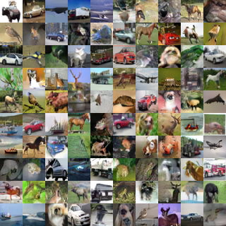
(a) CIFAR-10

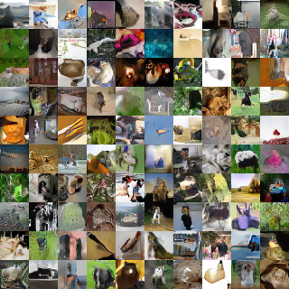
(b) ImageNet 32$\times$32

Figure 2: Unconditional generated samples from our EBMs on CIFAR-10 (Krizhevsky et al., 2009) and ImageNet 32$\times$32 (Deng et al., 2009; Chrabaszcz et al., 2017).

Table 4: AUROC scores in OOD detection using explicit density models on CIFAR-10. Bold and underline entries indicates the best and second best, respectively, among unsupervised methods, where JEM and VERA are supervised methods.

Method	SVHN	Textures	CIFAR10 Interp.	CIFAR100	CelebA
PixelCNN++ (Salimans et al., 2017)	0.32	0.33	0.71	0.63	-
GLOW (Kingma & Dhariwal, 2018)	0.24	0.27	0.51	0.55	0.57
NVAE (Vahdat & Kautz, 2020)	0.42	-	0.64	0.56	0.68
IGEBM (Du & Mordatch, 2019)	0.63	0.48	0.70	0.50	0.70
VAEBM (Xiao et al., 2021)	0.83	-	0.70	0.62	0.77
Improved CD (Du et al., 2021)	0.91	0.88	0.65	0.83	-
CLEL-Base (Ours)	0.9848	0.9437	0.7248	0.7161	0.7717
JEM (Grathwohl et al., 2019)	0.67	0.60	0.65	0.67	0.75
VERA (Grathwohl et al., 2021).	0.83	-	0.86	0.73	0.33

EBMs can be also used for detecting out-of-distribution (OOD) samples. For the OOD sample detection, previous EBM-based approaches often use the (marginal) unnormalized likelihood $p_{\theta}(\mathbf{x})\propto\exp(-E_{\theta}(\mathbf{x}))$. In contrast, our CLEL is capable of modeling the joint density $p_{\theta}(\mathbf{x},\mathbf{z})\propto E_{\theta}(\mathbf{x},\mathbf{z})$. Using this capability, we propose an energy-based OOD detection score: given $\mathbf{x}$,

$$s(\mathbf{x}):=\frac{1}{2}\lVert f_{\theta}(\mathbf{x})\rVert_{2}^{2}-\beta g_{\theta}\left(\frac{f_{\theta}(\mathbf{x})}{\lVert f_{\theta}(\mathbf{x})\rVert_{2}}\right)^{\top}\frac{h_{\phi}(\mathbf{x})}{\lVert h_{\phi}(\mathbf{x})\rVert_{2}}.$$ (14)

We found that the second term in (14) helps to detect the semantic difference between in- and out-of-distribution samples. Table 4 shows our CLEL’s superiority over other explicit density models in OOD detection, especially when OOD samples are drawn from different domains, e.g., SVHN (Netzer et al., 2011) and Texture (Cimpoi et al., 2014) datasets.

4.3 Conditional sampling

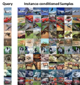
(a) Instance-conditional sampling

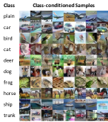
(b) Class-conditional sampling

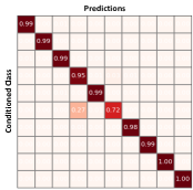
(c) Confusion matrix

Figure 3: (a, b) Instance- and class-conditionally generated samples using our CLEL in CIFAR-10. (c) Confusion matrix for the class-conditionally generated samples computed by an external classifier.

One advantage of latent-variable EBMs is that they can offer the latent-conditional density $p_{\theta}(\mathbf{x}|\mathbf{z})\propto\exp(-E_{\theta}(\mathbf{x},\mathbf{z}))$. Hence, our EBMs can enjoy the advantage even though CLEL does not explicitly train conditional models. To verify this, we first test instance-conditional sampling: given a real sample $\mathbf{x}$, we draw the underlying latent variable $\mathbf{z}\sim p_{\text{data}}(\mathbf{z}|\mathbf{x})$ using our latent encoder $h_{\phi}$, and then perform SGLD sampling using our joint energy $E_{\theta}(\mathbf{x},\mathbf{z})$ defined in (10). We here use our CIFAR-10 model. As shown in Figure 3(a), the instance-conditionally generated samples contain similar information (e.g., color, shape, and background) to the given instance.

This successful result motivates us to extend the sampling procedure: given a set of instances $\{\mathbf{x}^{(i)}\}$, can we generate samples that contain the shared information in $\{\mathbf{x}^{(i)}\}$? To this end, we first draw latent variables $\mathbf{z}^{(i)}\sim p_{\text{data}}(\cdot|\mathbf{x}^{(i)})$ for all $i$, and then aggregate them by summation and normalization: $\bar{\mathbf{z}}:=\sum_{i}\mathbf{z}^{(i)}/\lVert\sum_{i}\mathbf{z}^{(i)}\rVert_{2}$. To demonstrate that samples generated from $p_{\theta}(\mathbf{x}|\bar{\mathbf{z}})$ contains the shared information in $\{\mathbf{x}^{(i)}\}$, we collect the set of instances $\{\mathbf{x}^{(i)}_{y}\}$ for each label $y$ in CIFAR-10, and check whether $\tilde{\mathbf{x}}_{y}\sim p_{\theta}(\cdot|\bar{\mathbf{z}}_{y})$ has the same label $y$. Figure 3(b) shows the class-conditionally generated samples $\{\tilde{\mathbf{x}}_{y}\}$ and Figure 3(c) presents the confusion matrix of predictions for $\{\tilde{\mathbf{x}}_{y}\}$ computed by an external classifier $c$. Formally, each $(i,j)$-th entry is equal to $\mathbb{P}_{\tilde{\mathbf{x}}_{i}}(c(\tilde{\mathbf{x}}_{i})=j)$. We found that $\tilde{\mathbf{x}}_{y}$ is likely to be predicted as the label $y$, except the case when $y$ is dog: the generated dog images sometimes look like a semantically similar class, cat. These results verify that our EBM can generate samples conditioning on a instance or class label, even without explicit conditional training.

4.4 Compositionality via latent variables

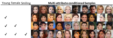
(a) Multi-attribute-conditional sampling

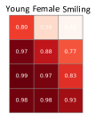
(b) Attribute predictions

Figure 4: Compositional generation results in CelebA. (a) Samples are generated by conditioning on checked attributes. (b) Attribute predictions of generated samples computed by an external classifier.

An intriguing property of EBMs is compositionality (Du et al., 2020a): given two EBMs $E(\mathbf{x}|c_{1})$ and $E(\mathbf{x}|c_{2})$ that are conditional energies on concepts $c_{1}$ and $c_{2}$, respectively, one can construct a new energy conditioning on both concepts: $p_{\theta}(\mathbf{x}|c_{1}\text{ and }c_{2})\propto\exp(-E(\mathbf{x}|c_{1})-E(\mathbf{x}|c_{2}))$. As shown in Section 4.3, our CLEL implicitly learns $E(\mathbf{x}|\mathbf{z})$, and a latent variable $\mathbf{z}$ can be considered as a concept, e.g., instance or class. Hence, in this section, we test compositionality of our model. To this end, we additionally train our CLEL in CelebA 64$\times$64 (Liu et al., 2015). For compositional sampling, we first acquire three attribute vectors $\bar{\mathbf{z}}_{a}$ for $a\in\mathcal{A}:=\{\text{Young},\text{Female},\text{Smiling}\}$ as we did in Section 4.3, then generate samples from a composition of conditional energies as follows:

$$E_{\theta}(\mathbf{x}|\mathcal{A}):=\frac{1}{2}\lVert f_{\theta}(\mathbf{x})\rVert_{2}-\beta\sum_{a\in\mathcal{A}}\text{sim}(g_{\theta}(f_{\theta}(\mathbf{x})/\lVert f_{\theta}(\mathbf{x})\rVert_{2}),\bar{\mathbf{z}}_{a}),$$ (15)

where $\text{sim}(\cdot,\cdot)$ is the cosine similarity. Figure 4(a) and 4(b) show the generated samples conditioning on multiple attributes and their attribute prediction results computed by an external classifier, respectively. They verify our compositionality qualitatively and quantitatively. For example, almost generated faces conditioned by $\{\text{Young},\text{Female}\}$ look young and female (see the third row in Figure 4.)

4.5 Ablation study

Component analysis. To verify the importance of our CLEL’s components, we conduct ablation experiments with training a smaller ResNet (He et al., 2016) in CIFAR-10 (Krizhevsky et al., 2009) for 50k training iterations. Then, we evaluate the quality of energy functions using FID and OOD detection scores. Here, we use SVHN (Netzer et al., 2011) as the OOD dataset. Table 7 demonstrates the effectiveness of CLEL’s components. First, we observe that learning $p_{\theta}(\mathbf{z}|\mathbf{x})$ to approximate $p_{\text{data}}(\mathbf{z}|\mathbf{x})$ plays a crucial role for improving generation (see (a) vs. (b)). In addition, using generated latent variables $\tilde{\mathbf{z}}\sim p_{\theta}(\cdot)$ as negatives for contrastive learning further improves not only generation, but also OOD detection performance (see (b) vs. (c)). We also empirically found that using an additional projection head is critical; without projection $g_{\theta}$ (i.e., (d)), our EBM failed to approximate $p_{\text{data}}(\mathbf{x})$, but an additional projection head (i.e., (c) or (e)) makes learning feasible. Hence, we use a 2-layer MLP (c) in all experiments since it is better than a simple linear function (e). We also test various $\beta\in\{0.1,0.01,0.001\}$ under this evaluation setup (see Table 7) and find $\beta=0.01$ is the best.

Compatibility with other self-supervised representation learning methods. While we have mainly focused on utilizing contrastive representation learning (CRL), our framework CLEL is not limited to CRL for learning the latent encoder $h_{\phi}$. To verify this compatibility, we replace SimCLR with other self-supervised representation learning (SSRL) methods, BYOL (Grill et al., 2020) and MAE (He et al., 2021). See Appendix C for implementation details. Note that these methods have several advantages compared to SimCLR: e.g., BYOL does not require negative pairs, and MAE does not require heavy data augmentations. Table 7 implies that any SSRL methods can be used to improve EBMs under our framework, where the CRL method, SimCLR (Chen et al., 2020), is the best.

Table 5: Component ablation experiments.

	Projection $g_{\theta}$	Negative $p_{\theta}(\tilde{\mathbf{z}})$	FID$\downarrow$	OOD$\uparrow$
(a)	Baseline ($\beta=0$)		42.46	0.8532
(b)	MLP		36.29	0.8580
(c)	MLP	✓	35.73	0.8723
(d)	Identity	✓	86.02	0.8474
(e)	Linear	✓	37.35	0.8540

Table 6: $\beta$ sensitivity.

$\beta$	FID$\downarrow$	OOD$\uparrow$
0	42.46	0.8532
0.001	37.44	0.8485
0.01	35.73	0.8723
0.1	56.39	0.7559

Table 7: Compatibility.

SSRL	FID$\downarrow$	OOD$\uparrow$
	42.46	0.8532
SimCLR	35.73	0.8723
BYOL	36.31	0.8792
MAE	37.67	0.8561

5 Related works

Energy-based models (EBMs) can offer an explicit density and are less restrictive in architecture design, but training them has been challenging. For example, it often suffers from the training instability due to the time-consuming and unstable MCMC sampling procedure (e.g., a large number of SGLD steps). To reduce the computational complexity and improve the quality of generated samples, various techniques have been proposed: a replay buffer (Du & Mordatch, 2019), short-run MCMC (Nijkamp et al., 2019), augmentation-based MCMC transitions (Du et al., 2021). Recently, researchers have also attempted to incorporate other generative frameworks into EBM training e.g., adversarial training (Kumar et al., 2019; Arbel et al., 2021; Grathwohl et al., 2021), flow-based models (Gao et al., 2020; Nijkamp et al., 2022; Xie et al., 2022), variational autoencoders (Xiao et al., 2021), and diffusion techniques (Gao et al., 2021). Another direction is on developing better divergence measures, e.g., $f$-divergence (Yu et al., 2020), pseudo-spherical scoring rule (Yu et al., 2021), and improved contrastive divergence (Du et al., 2021). Compared to the recent advances in the EBM literature, we have focused on an orthogonal research direction that investigates how to incorporate discriminative representations, especially of contrastive learning, into training EBMs.

6 Conclusion

The early advances in deep learning was initiated from the pioneering energy-based model (EBM) works, e.g., restricted and deep Boltzman machines (Salakhutdinov et al., 2007; Salakhutdinov & Hinton, 2009), however the recent accomplishments rather rely on other generative frameworks such as diffusion models (Ho et al., 2020; Song et al., 2021). To narrow the gap, in this paper, we suggest to utilize discriminative representations for improving EBMs, and achieve significant improvements. We hope that our work would shed light again on the potential of EBMs, and would guide many further research directions for EBMs.

Ethics statement

In recent years, generative models have been successful in synthesizing diverse high-fidelity images. However, high-quality image generation techniques have threats to be abused for unethical purposes, e.g., creating sexual photos of an individual. This significant threats call us researchers for the future efforts on developing techniques to detect such misuses. Namely, we should learn the data distribution $p(\mathbf{x})$ more directly. In this respect, learning explicit density models like VAEs and EBMs could be an effective solution. As we show the superior performance in both image generation and out-of-distribution detection, we believe that energy-based models, especially with discriminative representations, would be an important research direction for reliable generative modeling.

Reproducibility statement

We provide all the details to reproduce our experimental results in Appendix B. Our code is available at https://github.com/hankook/CLEL. In our experiments, we mainly use NVIDIA GTX3090 GPUs.

Appendix A Training procedure of CLEL

Algorithm 1 Contrastive Latent-guided Energy Learning (CLEL)

0:  a latent-variable EBM $(f_{\theta},g_{\theta})$, a latent encoder $h_{\phi}$, an augmentation distribution $\mathcal{T}$, hyperparameters $\alpha,\beta,\tau>0$, and the stop-gradient operation $\mathtt{sg}(\cdot)$.  

1:  for # training iterations do

2:     // Construct batches $\mathcal{B}$ and $\tilde{\mathcal{B}}$

3:     Sample $\{\mathbf{x}^{(i)}\}_{i=1}^{n}\sim p_{\text{data}}(\mathbf{x})$

4:     Sample $\{\tilde{\mathbf{x}}^{(i)}\}_{i=1}^{n}\sim p_{\theta}(\mathbf{x})$ using stochastic gradient Langevin dynamics (SGLD)

5:     $\mathbf{z}^{(i)}\leftarrow\mathtt{sg}\left(h_{\phi}(t^{(i)}(\mathbf{x}^{(i)}))/\lVert h_{\phi}(t^{(i)}(\mathbf{x}^{(i)}))\rVert_{2}\right)$, $t^{(i)}\sim\mathcal{T}$

6:     $\tilde{\mathbf{z}}^{(i)}\leftarrow\mathtt{sg}\left(g_{\theta}(f_{\theta}(\tilde{\mathbf{x}}^{(i)})/\lVert f_{\theta}(\tilde{\mathbf{x}}^{(i)})\rVert_{2})\right)$

7:     // Compute the EBM loss, $\mathcal{L}_{\text{EBM}}$

8:     $\mathcal{L}_{\text{EBM}}\leftarrow\frac{1}{n}\sum_{i=1}^{n}E_{\theta}(\mathbf{x}^{(i)},\mathbf{z}^{(i)})-E_{\theta}(\tilde{\mathbf{x}}^{(i)})+\alpha\cdot(E_{\theta}(\mathbf{x}^{(i)})^{2}+E_{\theta}(\tilde{\mathbf{x}}^{(i)})^{2})$

9:     // Compute the encoder loss, $\mathcal{L}_{\text{LE}}$

10:     $\mathbf{z}^{(i)}_{j}\leftarrow h_{\phi}(t^{(i)}_{j}(\mathbf{x}^{(i)}))$, $t^{(i)}_{j}\sim\mathcal{T}$

11:     $\mathcal{L}_{\text{LE}}\leftarrow\frac{1}{2n}\sum_{i=1}^{n}\sum_{j=1,2}\mathcal{L}_{\text{NT-Xent}}\left(\mathbf{z}^{(i)}_{j},\mathbf{z}^{(i)}_{3-j},\{\mathbf{z}_{l}^{(k)}\}_{k\neq i,l\in\{1,2\}}\cup\{\tilde{\mathbf{z}}^{(i)}\}_{i=1}^{n};\tau\right)$

12:     Update $\theta$ and $\phi$ to minimize $\mathcal{L}_{\text{EBM}}+\mathcal{L}_{\text{LE}}$

13:  end for

Appendix B Training details

Architectures. For the spherical latent-variable energy-based model (EBM) $f_{\theta}$, we use the 8-block ResNet (He et al., 2016) architectures following Du & Mordatch (2019). The details of the (a) small, (b) base, and (c) large ResNets are described in Table 8. We append a 2-layer MLP with a output dimension of 128 to the ResNet, i.e., $f_{\theta}:\mathbb{R}^{3\times 32\times 32}\rightarrow\mathbb{R}^{128}$. Note that we use the small model for ablation experiments in Section 4.5. To stabilize training, we apply spectral normalization (Miyato et al., 2018) to all convolutional layers. For the projection $g_{\theta}$, we use a 2-layer MLP with a output dimension of 128, the leaky-ReLU activation, and no bias, i.e., $g_{\theta}(\mathbf{u})=W_{2}\sigma(W_{1}\mathbf{u})\in\mathbb{R}^{128}$. For the latent encoder $h_{\phi}$, we simpy use the CIFAR variant of ResNet-18 (He et al., 2016), followed by a 2-layer MLP with a output dimension of 128.

Table 8: Our EBM $f_{\theta}$ architectures. For our large model, we build three independent ResNets and resize an input image $\mathbf{x}\in\mathbb{R}^{3\times 32\times 32}$ to three resolutions: $32\times 32$, $16\times 16$, and $8\times 8$. We use each ResNet for each resolution image, concatenate their output features, and then compute the final output feature $f_{\theta}(\mathbf{x})\in\mathbb{R}^{128}$ using single MLP.

	Small	Base	Large
Input	$(3,32,32)$	$(3,32,32)$	$(3,32,32)$, $(3,16,16)$, $(3,8,8)$
EBM $f_{\theta}(\mathbf{x})$	$\begin{matrix}\tt Conv(3\times 3,64)&\\ \tt ResBlock(64)&\times 1\\ \tt AvgPool(2\times 2)&\\ \tt ResBlock(64)&\times 1\\ \tt AvgPool(2\times 2)&\\ \tt ResBlock(128)&\times 1\\ \tt AvgPool(2\times 2)&\\ \tt ResBlock(128)&\times 1\\ \tt GlobalAvgPool&\\ \tt MLP(128,2048,128)&\end{matrix}$	$\begin{matrix}\tt Conv(3\times 3,128)&\\ \tt ResBlock(128)&\times 2\\ \tt AvgPool(2\times 2)&\\ \tt ResBlock(128)&\times 2\\ \tt AvgPool(2\times 2)&\\ \tt ResBlock(256)&\times 2\\ \tt AvgPool(2\times 2)&\\ \tt ResBlock(256)&\times 2\\ \tt GlobalAvgPool&\\ \tt MLP(256,2048,128)&\end{matrix}$	$\begin{matrix}\left\{\begin{matrix}\tt Conv(3\times 3,256)&\\ \tt ResBlock(256)&\times 2\\ \tt AvgPool(2\times 2)&\\ \tt ResBlock(256)&\times 2\\ \tt AvgPool(2\times 2)&\\ \tt ResBlock(256)&\times 2\\ \tt AvgPool(2\times 2)&\\ \tt ResBlock(256)&\times 2\\ \tt GlobalAvgPool&\\ \end{matrix}\right\}\times 3\\ \tt Concat\rightarrow MLP(768,2048,128)\end{matrix}$

Training. For the EBM parameter $\theta$, we use Adam optimizer (Kingma & Ba, 2015) with $\beta_{1}=0$, $\beta_{2}=0.999$, and a learning rate of $10^{-4}$. We use the linear learning rate warmup for the first 2k training iterations. For the encoder parameter $\phi$, we use SGD optimizer with a learning rate of $3\times 10^{-2}$, a weight decay of $5\times 10^{-4}$, and a momentum of $0.9$ as described in Chen & He (2020). For all experiments, we train our models up to 100k iterations with a batch size of 64, unless otherwise stated. For data augmentation $\mathcal{T}$, we follow Chen et al. (2020), i.e., $\mathcal{T}$ includes random cropping, flipping, color jittering, and color dropping. For hyperparameters, we use $\alpha=1$ following Du & Mordatch (2019), and $\beta=0.01$ (see Section 4.5 for $\beta$-sensitivity experiments). For our large model, we use a large batch size of $256$ only for learning the contrastive encoder $h_{\phi}$. After training, we utilize exponential moving average (EMA) models for evaluation.

SGLD sampling. For each training iteration, we use 60 SGLD steps with a step size of 100 for sampling $\tilde{\mathbf{x}}\sim p_{\theta}$. Following Du et al. (2021), we apply a random augmentation $t\sim\mathcal{T}$ for every 60 steps. We also use a replay buffer with a size of 10000 and a resampling rate of 0.1% for maintaining diverse samples (Du & Mordatch, 2019). For evaluation, we run 600 and 1200 SGLD steps from uniform noises for our base and large models, respectively.

Appendix C Implementation details for BYOL and MAE

We here provide implementation details for replacing SimCLR (Chen et al., 2020) with BYOL (Grill et al., 2020) and MAE (He et al., 2021) under our CLEL framework as shown in Section 4.5.

BYOL. Since BYOL also learns its representations on the unit sphere, the method can be directly incorporated with our CLEL framework.

MAE. Since MAE’s representations do not lie on the unit sphere, we incorporate MAE into our CLEL framework by the following procedure:

1. Pretrain a MAE framework and remove its MAE decoder. To this end, we simply use a publicly-available checkpoint of the ViT-tiny architecture.

2. Freeze the MAE encoder parameters and construct a learnable 2-layer MLP on the top of the encoder.

3. Train only the MLP via contrastive representation learning without data augmentations using our objective (13) for the latent encoder.

Appendix D Training stability with norm-direction separation

(a) Multi-head architecture

(b) Norm-direction separation

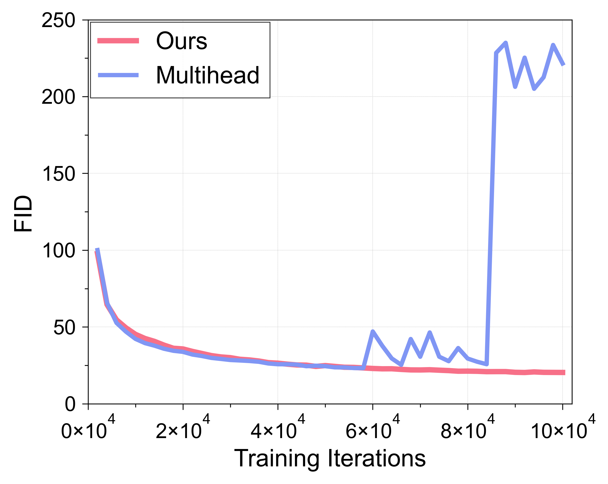
(c) FID scores during training

Figure 5: (a) A multi-head architecture design and (b) our norm-direction separation scheme for modeling $p(\mathbf{x})$ and $p(\mathbf{z}|\mathbf{x})$. (c) FID scores with various energy design choices.

At the early stage of our research, we first tested a multi-head architecture for modeling $p(\mathbf{x})$ and $p(\mathbf{z}|\mathbf{x})$. To be specific, $E(\mathbf{x})=g^{\prime}_{\theta}(f_{\theta}(\mathbf{x}))\in\mathbb{R}$ and $E(\mathbf{z}|\mathbf{x})=\mathbf{z}^{\top}g_{\theta}(f(\mathbf{x}))$ where $f$ is a shared backbone and $g$ and $g^{\prime}$ are separate 2-layer MLPs, as shown in Figure 5(a). We found that, with this choice, learning $p(\mathbf{x})$ causes a mode collapse for $f_{\theta}(\mathbf{x})$ because all samples should be aligned with a specific direction. In contrast, learning $p(\mathbf{z}|\mathbf{x})$ encourages $f_{\theta}(\mathbf{x})$ to be diverse due to contrastive learning. Namely, modeling $p(\mathbf{x})$ and $p(\mathbf{z}|\mathbf{x})$ with the multi-head architecture makes some conflict during optimization. We empirically observe that the multi-head architecture is unstable in EBM training, as shown in Figure 5(c). To remove such a conflict, we design the norm-direction separation for modeling p(x) and p(z|x) simultaneously (i.e., Figure 5(b)), which leads to training stability, as shown in Figure 5(c).

Appendix E The role of directional projector

(a) $f_{\theta}(\mathbf{x})$

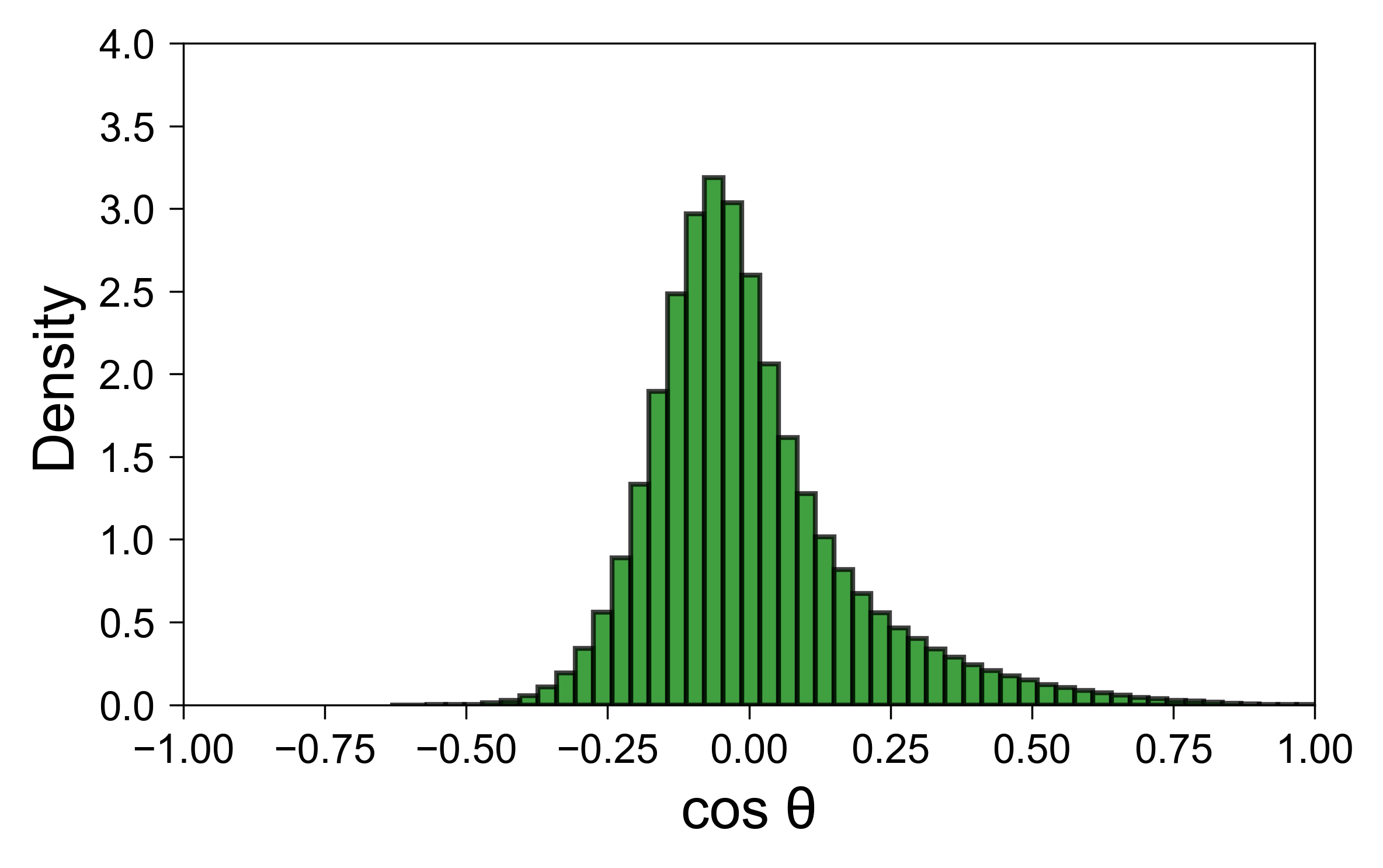
(b) $g_{\theta}(f_{\theta}(\mathbf{x}))$

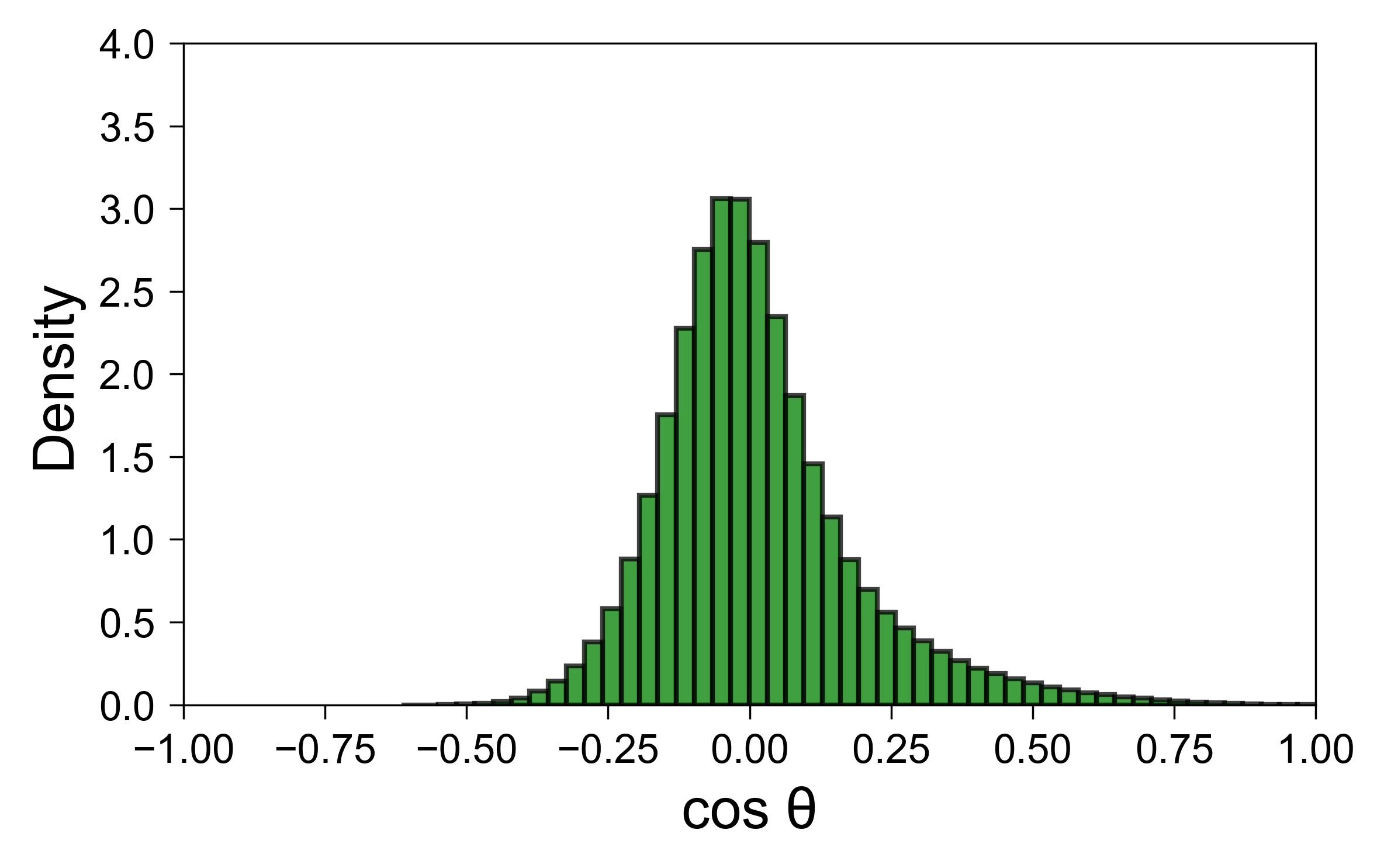
(c) $h_{\phi}(\mathbf{x})$

Figure 6: Cosine similarity distributions using (a) $f_{\theta}(\mathbf{x})$, (b) $g_{\theta}(f_{\theta}(\mathbf{x}))$, and (c) $h_{\phi}(\mathbf{x})$ features.

Our directional projector $g_{\theta}$ is designed for narrowing the gap between the EBM feature direction $f_{\theta}(\mathbf{x})/\lVert f_{\theta}(\mathbf{x})\rVert_{2}$ and the “uniformly-distributed” latent variable $p_{\text{data}}(\mathbf{z})$ (i.e., $h_{\theta}(\mathbf{x})/\lVert h_{\theta}(\mathbf{x})\rVert_{2}$). Specifically, the contrastive latent variable $p_{\text{data}}(\mathbf{z})$ is known to be uniformly distributed (Wang & Isola, 2020), but we observed that it is difficult to optimize the feature direction $f_{\theta}(\mathbf{x})/\lVert f_{\theta}(\mathbf{x})\rVert_{2}$ to be uniform along with learning our norm-based EBM $p_{\theta}(\mathbf{x})\propto\exp(-\lVert f_{\theta}(\mathbf{x})\rVert_{2}^{2})$ at the same time. As empirical supports, we analyze the cosine similarity distributions using $f_{\theta}(\mathbf{x})$, $g_{\theta}(f_{\theta}(\mathbf{x}))$, and $h_{\phi}(\mathbf{x})$ features on CIFAR-10, as shown in Figure 6. This figure shows that $f_{\theta}(\mathbf{x})$ tends to learn similar directions (see Figure 6(a)) while $h_{\phi}(\mathbf{x})$ tends to be uniformly distributed (see Figure 6(c)). Hence, it is necessary to employ a projection between them. We found that our projector $g_{\theta}$ successfully narrows the gap as shown in Figure 6(b), which significantly improves training EBMs.

Appendix F Flexibility of norm-based energy function

Our norm-based energy parametrization does not sacrifice the flexibility compared to the vanilla parametrization of EBMs. We here show that any vanilla EBM $p_{1}(\mathbf{x})\propto\exp(f_{1}(\mathbf{x}))$, $f_{1}(\mathbf{x})\in\mathbb{R}$, can be formulated by a norm-based EBM $p_{2}(\mathbf{x})\propto\exp(\lVert f_{2}(\mathbf{x})\rVert_{2}^{2})$, $f_{2}(\mathbf{x})\in\mathbb{R}^{d}$, on a compact input space $\mathcal{X}$ (e.g., an image $\mathbf{x}$ lies on the continuous pixel space $\mathcal{X}=[0,255]^{HWC}$).

Let $b:=\min_{\mathbf{x}\in\mathcal{X}}f_{1}(\mathbf{x})$ be the minimum value of $f_{1}$. Then, $p_{3}(\mathbf{x})\propto\exp(f_{1}(\mathbf{x})-b)$ is identical to $p_{1}$ due to the normalizing constant. Furthermore, $p_{3}$ can be formulated as a special case of the norm-based EBM $p_{2}$: for example, if the first component of $f_{2}$ is the same as $\sqrt{f_{1}(\mathbf{x})-b}$ and other components are zero, then $p_{1}$ and $p_{2}$ model the exactly same distribution. Therefore, energy-modeling with our norm-based design is not much different from that with the vanilla form.

References

- Aneja et al. (2021) Jyoti Aneja, Alex Schwing, Jan Kautz, and Arash Vahdat. A contrastive learning approach for training variational autoencoder priors. In Advances in neural information processing systems, 2021.
- Arbel et al. (2021) Michael Arbel, Liang Zhou, and Arthur Gretton. Generalized energy based models. In International Conference on Learning Representations, 2021.
- Bang & Shim (2021) Duhyeon Bang and Hyunjung Shim. Mggan: Solving mode collapse using manifold-guided training. In Proceedings of the IEEE/CVF international conference on computer vision, 2021.
- Chen et al. (2020) Ting Chen, Simon Kornblith, Mohammad Norouzi, and Geoffrey Hinton. A simple framework for contrastive learning of visual representations. In International Conference on Machine Learning, 2020.
- Chen & He (2020) Xinlei Chen and Kaiming He. Exploring simple siamese representation learning. arXiv preprint arXiv:2011.10566, 2020.
- Chrabaszcz et al. (2017) Patryk Chrabaszcz, Ilya Loshchilov, and Frank Hutter. A downsampled variant of imagenet as an alternative to the cifar datasets. arXiv preprint arXiv:1707.08819, 2017.
- Cimpoi et al. (2014) Mircea Cimpoi, Subhransu Maji, Iasonas Kokkinos, Sammy Mohamed, and Andrea Vedaldi. Describing textures in the wild. In Proceedings of the IEEE Conference on Computer Vision and Pattern Recognition, pp. 3606–3613, 2014.
- Deng et al. (2009) Jia Deng, Wei Dong, Richard Socher, Li-Jia Li, Kai Li, and Li Fei-Fei. Imagenet: A large-scale hierarchical image database. In IEEE Conference on Computer Vision and Pattern Recognition, pp. 248–255, 2009.
- Deng et al. (2020) Yuntian Deng, Anton Bakhtin, Myle Ott, Arthur Szlam, and Marc’Aurelio Ranzato. Residual energy-based models for text generation. In International Conference on Learning Representations, 2020.
- Dinh et al. (2017) Laurent Dinh, Jascha Sohl-Dickstein, and Samy Bengio. Density estimation using real nvp. In International Conference on Learning Representations, 2017.
- Du & Mordatch (2019) Yilun Du and Igor Mordatch. Implicit generation and generalization in energy-based models. In Advances in Neural Information Processing Systems, 2019.
- Du et al. (2020a) Yilun Du, Shuang Li, and Igor Mordatch. Compositional visual generation with energy based models. In Advances in Neural Information Processing Systems, 2020a.
- Du et al. (2020b) Yilun Du, Joshua Meier, Jerry Ma, Rob Fergus, and Alexander Rives. Energy-based models for atomic-resolution protein conformations. In International Conference on Learning Representations, 2020b.
- Du et al. (2021) Yilun Du, Shuang Li, Joshua Tenenbaum, and Igor Mordatch. Improved contrastive divergence training of energy based models. In International Conference on Machine Learning, 2021.
- Gao et al. (2020) Ruiqi Gao, Erik Nijkamp, Diederik P Kingma, Zhen Xu, Andrew M Dai, and Ying Nian Wu. Flow contrastive estimation of energy-based models. In Proceedings of the IEEE/CVF Conference on Computer Vision and Pattern Recognition, pp. 7518–7528, 2020.
- Gao et al. (2021) Ruiqi Gao, Yang Song, Ben Poole, Ying Nian Wu, and Diederik P Kingma. Learning energy-based models by diffusion recovery likelihood. In International Conference on Learning Representations, 2021.
- Goodfellow et al. (2014) Ian Goodfellow, Jean Pouget-Abadie, Mehdi Mirza, Bing Xu, David Warde-Farley, Sherjil Ozair, Aaron Courville, and Yoshua Bengio. Generative adversarial nets. In Advances in neural information processing systems, 2014.
- Grathwohl et al. (2019) Will Grathwohl, Kuan-Chieh Wang, Joern-Henrik Jacobsen, David Duvenaud, Mohammad Norouzi, and Kevin Swersky. Your classifier is secretly an energy based model and you should treat it like one. In International Conference on Learning Representations, 2019.
- Grathwohl et al. (2021) Will Sussman Grathwohl, Jacob Jin Kelly, Milad Hashemi, Mohammad Norouzi, Kevin Swersky, and David Duvenaud. No mcmc for me: Amortized sampling for fast and stable training of energy-based models. In International Conference on Learning Representations, 2021.
- Grill et al. (2020) Jean-Bastien Grill, Florian Strub, Florent Altché, Corentin Tallec, Pierre H Richemond, Elena Buchatskaya, Carl Doersch, Bernardo Avila Pires, Zhaohan Daniel Guo, Mohammad Gheshlaghi Azar, et al. Bootstrap Your Own Latent: A new approach to self-supervised learning. arXiv preprint arXiv:2006.07733, 2020.
- He et al. (2016) Kaiming He, Xiangyu Zhang, Shaoqing Ren, and Jian Sun. Deep residual learning for image recognition. In Proceedings of the IEEE Conference on Computer Vision and Pattern Recognition, pp. 770–778, 2016.
- He et al. (2020) Kaiming He, Haoqi Fan, Yuxin Wu, Saining Xie, and Ross Girshick. Momentum contrast for unsupervised visual representation learning. In Proceedings of the IEEE/CVF Conference on Computer Vision and Pattern Recognition, 2020.
- He et al. (2021) Kaiming He, Xinlei Chen, Saining Xie, Yanghao Li, Piotr Dollár, and Ross Girshick. Masked autoencoders are scalable vision learners, 2021.
- Hendrycks et al. (2019a) Dan Hendrycks, Kimin Lee, and Mantas Mazeika. Using pre-training can improve model robustness and uncertainty. In International Conference on Machine Learning, pp. 2712–2721. PMLR, 2019a.
- Hendrycks et al. (2019b) Dan Hendrycks, Mantas Mazeika, Saurav Kadavath, and Dawn Song. Using self-supervised learning can improve model robustness and uncertainty. Advances in neural information processing systems, 32, 2019b.
- Heusel et al. (2017) Martin Heusel, Hubert Ramsauer, Thomas Unterthiner, Bernhard Nessler, and Sepp Hochreiter. Gans trained by a two time-scale update rule converge to a local nash equilibrium. In Advances in neural information processing systems, 2017.
- Ho et al. (2020) Jonathan Ho, Ajay Jain, and Pieter Abbeel. Denoising diffusion probabilistic models. In Advances in Neural Information Processing Systems, 2020.
- Ingraham et al. (2019) John Ingraham, Adam Riesselman, Chris Sander, and Debora Marks. Learning protein structure with a differentiable simulator. In International Conference on Learning Representations, 2019.
- Jeong & Shin (2021) Jongheon Jeong and Jinwoo Shin. Training {gan}s with stronger augmentations via contrastive discriminator. In International Conference on Learning Representations, 2021.
- Jerrum & Sinclair (1993) Mark Jerrum and Alistair Sinclair. Polynomial-time approximation algorithms for the ising model. SIAM Journal on Computing, 22(5):1087–1116, 1993.
- Kan et al. (2022) Ge Kan, Jinhu Lü, Tian Wang, Baochang Zhang, Aichun Zhu, Lei Huang, Guodong Guo, and Hichem Snoussi. Bi-level doubly variational learning for energy-based latent variable models. In Proceedings of the IEEE/CVF Conference on Computer Vision and Pattern Recognition, 2022.
- Kang et al. (2021) Minguk Kang, Woohyeon Shim, Minsu Cho, and Jaesik Park. Rebooting acgan: Auxiliary classifier gans with stable training. In Advances in Neural Information Processing Systems, 2021.
- Karras et al. (2020) Tero Karras, Miika Aittala, Janne Hellsten, Samuli Laine, Jaakko Lehtinen, and Timo Aila. Training generative adversarial networks with limited data, 2020.
- Kingma & Ba (2015) Diederik P Kingma and Jimmy Ba. Adam: A method for stochastic optimization. In International Conference on Learning Representations, 2015.
- Kingma & Dhariwal (2018) Durk P Kingma and Prafulla Dhariwal. Glow: Generative flow with invertible 1x1 convolutions. In Advances in neural information processing systems, 2018.
- Krizhevsky et al. (2009) Alex Krizhevsky, Geoffrey Hinton, et al. Learning multiple layers of features from tiny images. Technical report, University of Toronto, 2009.
- Kumar et al. (2019) Rithesh Kumar, Sherjil Ozair, Anirudh Goyal, Aaron Courville, and Yoshua Bengio. Maximum entropy generators for energy-based models. arXiv preprint arXiv:1901.08508, 2019.
- LeCun et al. (2006) Yann LeCun, Sumit Chopra, Raia Hadsell, M Ranzato, and F Huang. A tutorial on energy-based learning. Predicting structured data, 1(0), 2006.
- Liu et al. (2015) Ziwei Liu, Ping Luo, Xiaogang Wang, and Xiaoou Tang. Deep learning face attributes in the wild. In International Conference on Computer Vision, December 2015.
- Mirza & Osindero (2014) Mehdi Mirza and Simon Osindero. Conditional generative adversarial nets. arXiv preprint arXiv:1411.1784, 2014.
- Miyato et al. (2018) Takeru Miyato, Toshiki Kataoka, Masanori Koyama, and Yuichi Yoshida. Spectral normalization for generative adversarial networks. In International Conference on Learning Representations, 2018.
- Netzer et al. (2011) Yuval Netzer, Tao Wang, Adam Coates, Alessandro Bissacco, Bo Wu, and Andrew Y Ng. Reading digits in natural images with unsupervised feature learning. In NIPS Workshop on Deep Learning and Unsupervised Feature Learning, 2011.
- Nijkamp et al. (2019) Erik Nijkamp, Mitch Hill, Song-Chun Zhu, and Ying Nian Wu. Learning non-convergent non-persistent short-run mcmc toward energy-based model. In Advances in Neural Information Processing Systems, 2019.
- Nijkamp et al. (2022) Erik Nijkamp, Ruiqi Gao, Pavel Sountsov, Srinivas Vasudevan, Bo Pang, Song-Chun Zhu, and Ying Nian Wu. MCMC should mix: Learning energy-based model with neural transport latent space MCMC. In International Conference on Learning Representations, 2022.
- Odena et al. (2017) Augustus Odena, Christopher Olah, and Jonathon Shlens. Conditional image synthesis with auxiliary classifier gans. In International conference on machine learning, 2017.
- Oord et al. (2016a) Aaron van den Oord, Sander Dieleman, Heiga Zen, Karen Simonyan, Oriol Vinyals, Alex Graves, Nal Kalchbrenner, Andrew Senior, and Koray Kavukcuoglu. Wavenet: A generative model for raw audio. arXiv preprint arXiv:1609.03499, 2016a.
- Oord et al. (2016b) Aaron van den Oord, Nal Kalchbrenner, and Koray Kavukcuoglu. Pixel recurrent neural networks. In International Conference on Machine Learning, 2016b.
- Oord et al. (2018) Aaron van den Oord, Yazhe Li, and Oriol Vinyals. Representation learning with contrastive predictive coding. arXiv preprint arXiv:1807.03748, 2018.
- Raginsky et al. (2017) Maxim Raginsky, Alexander Rakhlin, and Matus Telgarsky. Non-convex learning via stochastic gradient langevin dynamics: a nonasymptotic analysis. In Conference on Learning Theory, pp. 1674–1703. PMLR, 2017.
- Reed et al. (2016) Scott Reed, Zeynep Akata, Xinchen Yan, Lajanugen Logeswaran, Bernt Schiele, and Honglak Lee. Generative adversarial text to image synthesis. In International conference on machine learning, pp. 1060–1069, 2016.
- Rezende & Mohamed (2015) Danilo Rezende and Shakir Mohamed. Variational inference with normalizing flows. In International Conference on Machine Learning, 2015.
- Salakhutdinov & Hinton (2009) Ruslan Salakhutdinov and Geoffrey Hinton. Deep boltzmann machines. In Proceedings of the Twelth International Conference on Artificial Intelligence and Statistics, volume 5 of Proceedings of Machine Learning Research, pp. 448–455, 2009.
- Salakhutdinov et al. (2007) Ruslan Salakhutdinov, Andriy Mnih, and Geoffrey Hinton. Restricted boltzmann machines for collaborative filtering. In International Conference on Machine Learning, 2007.
- Salimans et al. (2017) Tim Salimans, Andrej Karpathy, Xi Chen, and Diederik P Kingma. Pixelcnn++: Improving the pixelcnn with discretized logistic mixture likelihood and other modifications. arXiv preprint arXiv:1701.05517, 2017.
- Seitzer (2020) Maximilian Seitzer. pytorch-fid: FID Score for PyTorch. https://github.com/mseitzer/pytorch-fid, August 2020. Version 0.2.1.
- Song & Ermon (2019) Yang Song and Stefano Ermon. Generative modeling by estimating gradients of the data distribution. In Advances in Neural Information Processing Systems, 2019.
- Song & Ermon (2020) Yang Song and Stefano Ermon. Improved techniques for training score-based generative models. In Advances in neural information processing systems, 2020.
- Song et al. (2021) Yang Song, Jascha Sohl-Dickstein, Diederik P Kingma, Abhishek Kumar, Stefano Ermon, and Ben Poole. Score-based generative modeling through stochastic differential equations. In International Conference on Learning Representations, 2021.
- Tack et al. (2020) Jihoon Tack, Sangwoo Mo, Jongheon Jeong, and Jinwoo Shin. Csi: Novelty detection via contrastive learning on distributionally shifted instances. In Advances in Neural Information Processing Systems, 2020.
- Tian et al. (2019) Yonglong Tian, Dilip Krishnan, and Phillip Isola. Contrastive multiview coding. arXiv preprint arXiv:1906.05849, 2019.
- Tian et al. (2020) Yonglong Tian, Chen Sun, Ben Poole, Dilip Krishnan, Cordelia Schmid, and Phillip Isola. What makes for good views for contrastive learning? In Advances in Neural Information Processing Systems, 2020.
- Vahdat & Kautz (2020) Arash Vahdat and Jan Kautz. Nvae: A deep hierarchical variational autoencoder. In Advances in Neural Information Processing Systems, 2020.
- Vahdat et al. (2021) Arash Vahdat, Karsten Kreis, and Jan Kautz. Score-based generative modeling in latent space. In Advances in Neural Information Processing Systems, 2021.
- Van den Oord et al. (2016) Aaron Van den Oord, Nal Kalchbrenner, Lasse Espeholt, Oriol Vinyals, Alex Graves, et al. Conditional image generation with pixelcnn decoders. In Advances in neural information processing systems, 2016.
- Vollmer et al. (2016) Sebastian J Vollmer, Konstantinos C Zygalakis, and Yee Whye Teh. Exploration of the (non-) asymptotic bias and variance of stochastic gradient langevin dynamics. The Journal of Machine Learning Research, 17(1):5504–5548, 2016.
- Wang & Isola (2020) Tongzhou Wang and Phillip Isola. Understanding contrastive representation learning through alignment and uniformity on the hypersphere. In International Conference on Machine Learning, 2020.
- Welling & Teh (2011) Max Welling and Yee W Teh. Bayesian learning via stochastic gradient Langevin dynamics. In International Conference on Machine Learning, 2011.
- Wu et al. (2021) Hao Wu, Babak Esmaeili, Michael Wick, Jean-Baptiste Tristan, and Jan-Willem van de Meent. Conjugate energy-based models. In International Conference on Machine Learning, 2021.
- Xiao et al. (2021) Zhisheng Xiao, Karsten Kreis, Jan Kautz, and Arash Vahdat. Vaebm: A symbiosis between variational autoencoders and energy-based models. In International Conference on Learning Representations, 2021.
- Xie et al. (2022) Jianwen Xie, Yaxuan Zhu, Jun Li, and Ping Li. A tale of two flows: Cooperative learning of langevin flow and normalizing flow toward energy-based model. In International Conference on Learning Representations, 2022. URL https://openreview.net/forum?id=31d5RLCUuXC.
- Xu et al. (2018) Pan Xu, Jinghui Chen, Difan Zou, and Quanquan Gu. Global convergence of langevin dynamics based algorithms for nonconvex optimization. Advances in Neural Information Processing Systems, 2018.
- Yang & Ji (2021) Xiulong Yang and Shihao Ji. Jem++: Improved techniques for training jem. In International Conference on Computer Vision, 2021.
- Yu et al. (2020) Lantao Yu, Yang Song, Jiaming Song, and Stefano Ermon. Training deep energy-based models with f-divergence minimization. In International Conference on Machine Learning, 2020.
- Yu et al. (2021) Lantao Yu, Jiaming Song, Yang Song, and Stefano Ermon. Pseudo-spherical contrastive divergence. In Advances in Neural Information Processing Systems, 2021.
- Zhao et al. (2020) Shengyu Zhao, Zhijian Liu, Ji Lin, Jun-Yan Zhu, and Song Han. Differentiable augmentation for data-efficient gan training. In Advances in Neural Information Processing Systems, 2020.
- Zhao et al. (2021) Yang Zhao, Jianwen Xie, and Ping Li. Learning energy-based generative models via coarse-to-fine expanding and sampling. In International Conference on Learning Representations, 2021.
- Zou et al. (2021) Difan Zou, Pan Xu, and Quanquan Gu. Faster convergence of stochastic gradient Langevin dynamics for non-log-concave sampling. In Uncertainty in Artificial Intelligence, 2021.