Identification of Ex ante Returns Using Elicited Choice Probabilities

Abstract.

This paper studies the identification of perceived ex ante returns in the context of binary human capital investment decisions. The environment is characterised by uncertainty about future outcomes, with some uncertainty being resolved over time. In this context, each individual holds a probability distribution over different levels of returns. The paper uses the hypothetical choice methodology to identify nonparametrically the population distribution of several individual-specific distribution parameters, which are crucial for counterfactual policy analyses. The empirical application estimates perceived returns on overstaying for Afghan asylum seekers in Germany and evaluates the effect of assisted voluntary return policies.

Keywords: Subjective expectations; ex ante returns; nonparametric; semiparametric; distribution regression; asylum seekers.

JEL codes: C20, D84, F22, J15, J18, J61, O15.

1. Introduction

A is an asylum seeker whose asylum claim has been rejected and is required to leave her host country within 30 days. When asked by a researcher: ‘what is the chance that you will overstay at the end of the 30-day grace period?’, she answers 60 percent. A’s answer conveys at least two information: (1) her perception about the returns on overstaying at the time she will take the decision, and (2) her uncertainty about possible changes in this perception between the time she is asked about her future decision, and the time she will take the actual decision 30 days later.

A’s perception of returns at the time of elicitation is known as her ex ante returns. These returns encompass both perceived pecuniary and non-pecuniary benefits attached to her choice as compared to her next best alternative. They can be measured by the pecuniary transfer that would make A indifferent between staying and leaving. Because of the uncertainty about possible shocks between the time of elicitation and the time of decision, A’s ex ante returns are best described by a probability distribution over different levels of returns. This probability distribution is individual-specific and is characterised by distribution parameters: mean, spread, or more generally, quantiles. Furthermore, each asylum seeker sharing A’s circumstances holds such private distribution of ex ante returns. Thus, aggregated at the population level, there exists a population distribution of individual-specific distribution parameters.

In recent years, probabilistic stated choice questions similar to or more complex than the one described above have become widely applied to understand individuals’ ex ante returns about several human capital decisions (e.g., education, major and career choices, migration and retirement decisions) and more general economic choices. These applications pioneered by Blass et al., (2010) have largely focused on understanding mean ex ante returns and marginal effect of choice characteristics on mean returns. In an innovative contribution, Wiswall and Zafar, (2018) derived estimates of the population distribution of marginal mean returns of workplace attributes (or equivalently willingness-to-pay for these attributes).

Much less effort has been devoted to go beyond mean returns and understand the whole private distribution of ex ante returns. Yet, there exists two compelling arguments for going beyond the mean. First, for the purpose of describing individuals’ ex ante returns, distribution parameters such as quantiles give a more complete representation of both perceived returns and the associated uncertainty in the population. For example, whereas the population distribution of median ex ante returns reveals ‘typical’ expected returns, the distributions of upper and lower quantiles inform us on the whole range of returns that agents expect, and to which extent they perceive these returns as plausible. Moreover, the distribution of spreads describes the prevalence of uncertainty in the population. Finally, as the importance that agents put on some choice attributes can vary if they experience a ‘bad shock’ (low quantiles) or a ‘good’ shock (high quantiles), it is essential to investigate quantile effects as well as mean effects of choice characteristics.

Second, for the purpose of policy evaluation, one goal of stated preference analyses is to predict individuals’ outcomes and choice behaviour as a result of a (policy) change in their environment. Relying on an analysis of mean returns, although simple, can be short-sighted. High uncertainty signals that agents expect important variations in their ex ante perception and the mean might not be very informative about their outcome or future choice. Instead, understanding the whole private distribution of ex ante returns can be an important asset. More specifically, at the time of decision, the resolution of uncertainty will generate a mixture of shocks in the population. For some individuals, the realised uncertainty will correspond to the first quantile of their expectations, for others to the second quantile, to the third and so on. Thus, if preferences are stable, the realised distribution of returns, the main device for counterfactual analyses, will be a mixture of the distributions of quantile. The latter does not necessarily correspond to the distribution of mean (or median) returns. Yet, it can be estimated from the distributions of quantile, for any given prior of the policy maker about the accuracy of individuals’ perception. Thus, going beyond mean returns to identify distributions of quantile appears quintessential for careful policy evaluation.

The paper derives nonparametric identification results for the distribution of individual-specific quantiles, quantile effects, mean returns, mean effects, and spread of resolvable uncertainty. To the best of my knowledge, this is the first paper to propose a nonparametric characterisation and identification of these objects. They are defined formally in Section 3. For ease of language, they are referred to as to the population distributions of interest rather than as to the population distributions of individual-specific distribution parameters.

The identification result applies to a general model of human capital investment with uncertainty, for which the introductory example about the decision to overstay provides a prototypical illustration. Individuals make a binary investment choice (overstay or leave) in an environment characterised by uncertainty about their future outcomes (earning some income in the host country, being deported, becoming regularised). Some but not all uncertainty is resolved at the time of decision. In this context, individuals form subjective expectations about their outcomes and the nature of uncertainty. Further examples of related decisions include education investment, health investment, college major or occupation choices, job search, mobility and retirement decisions.

The paper considers the identification of the distributions of interest from the perspective of a (probabilistic) stated choice analysis (or stated preference analysis). Contrary to the revealed preference approach, which relies on observation of actual choices, the stated preference approach elicits individuals’ intended choice, often in hypothetical scenarios, alongside beliefs about choice characteristics (or attributes). The increasing interest in the stated preference approach stems from its advantages over the revealed preference approach. It avoids assumptions about agents’ belief formation and equilibrium allocation mechanisms, while being a more natural approach to questions pertaining to ex ante perceptions. Researchers can exploit hypothetical choice scenarios in stated choice analyses to tackle the pervasive problem of endogeneity arising because not all relevant beliefs and characteristics can be observed.

A key contribution of the present paper is to demonstrate a further advantage of the stated preference analysis: it can recover rich information on individuals’ perception of returns and resolvable uncertainty. The literature on probabilistic stated choice has devoted little attention to the potential insights on individual-specific distribution parameters so far. Yet, these distribution parameters are useful for forming a better understanding of agent choices and essential for appropriate counterfactual analyses.

As a second contribution, the paper shows nonparametric identification of the population distributions of interest under mild assumptions and for a simple elicitation design. This is a significant contribution to the stated preference literature, which relies almost exclusively on parametric assumptions about individuals’ utility function and the resolvable uncertainty. The benefits and limitations of the parametric approach are discussed in Section 2.

In this paper, identification of the distributions of interest proceeds in two steps. In a first step, Section 4.1 shows that the population distributions of interest can be written as functional of two structural objects: (i) the structural function that maps observed and unobserved beliefs and characteristics into individuals’ probabilistic choices, and (ii) the joint distribution of observed and unobserved beliefs and characteristics. The main assumption is that there exists a set of traits and information, potentially unobserved, that determine the distribution of resolvable uncertainty. The characterisation result relates to a similar characterisation of the marginal distributions of equivalent variation and compensation variation in discrete choice models by Bhattacharya, (2015) (Theorem 1, p. 626).

In a second step, Section 4.2 shows that (i) and (ii) are recoverable from the joint distribution of intended choice and observed beliefs for a simple elicitation strategy and under mild assumptions. The elicitation strategy is as follows: the researcher elicits both actual beliefs and intentions and beliefs and intentions in a limited number of counterfactual/hypothetical scenarios. At least one of the hypothetical scenarios is common to all respondents. Hence, the data required for identification is similar to the data routinely collected for generic probabilistic stated choice analyses, except for the need of at least one common scenario. For example, as long as one common scenario is introduced, the identification and estimation procedures can accommodate the common elicitation strategy where scenarios are anchored in individuals’ actual experience and only the extent of departures from this scenario varies experimentally.

When the unobserved heterogeneity can be summarised by a unidimensional random variable, the identification problem translates into the identification of a nonadditive panel model with an individual fixed effect. One common hypothetical scenario is enough for identification. In this case, the identification result can be seen as an application of existing identification results in panel models with nonseparable fixed effects and classical measurement error on the outcome variable, in particular, the result of Evdokimov, (2010). The novelty is the application of the latter result to models of stated preference with data generated from a pseudo-panel.

When the unobserved heterogeneity is multidimensional, a random coefficient representation is introduced to model the quantile functions of (i) and (ii). Under this assumption, when the unobserved heterogeneity is two-dimensional, two common hypothetical scenarios are enough, when three-dimensional, three scenarios, and so forth. Thus, by introducing several hypothetical scenarios, one can consider a larger dimension of unobserved heterogeneity. In this case, the identification result extends the result of Evdokimov, (2010).

The third methodological contribution is a tractable estimation procedure introduced in Section 5. Starting from the constructive proof of identification, the paper provides a semiparametric procedure that builds on recent developments in distribution regression estimators such as Chernozhukov et al., (2013), Melly and Santangelo, (2015) and Chernozhukov et al., (2020). In particular, in the case where the measurement error of the stated intention is negligible, it supplies a very simple two-stage estimator to recover the distributions of quantile in the population. To account for measurement error of these stated intention, the paper proposes an equally tractable bound approach that preserves the simplicity of the estimator. Inference uses a weighted bootstrap procedure, for which an asymptotic theory is developed in Appendix D.

The main advantages of the proposed approach are the following:

1. There is no need to impose a parametric and/or common distribution of the resolvable uncertainty.

2. There is no need to assume linearity and separability of individuals’ utility.

3. The number of hypothetical scenarios can remain limited and depends on the extent of unobserved heterogeneity one wishes to consider.

4. Estimation is feasible with usual econometric tools.

5. One can easily go beyond an analysis of mean and analyse quantiles of returns within the same econometric framework.

Thus, the proposed approach complements well the existing approaches in the stated preference literature presented in Section 2. It is especially appropriate when the researcher is unwilling to impose strong parametric assumptions, is interested in parameters derived from the resolvable uncertainty, needs to limit the number of counterfactual scenarios, or wishes to assess the sensitivity of their findings to parametric assumptions. Finally, it permits richer counterfactual analyses as illustrated in the empirical application.

The final contribution of the paper is empirical. The framework is used to estimate asylum seekers’ perceived returns on overstaying, with unique data on Afghan asylum seekers in Germany, the largest group of overstayers in the country. Section 6 gives unprecedented insights on the ex ante returns for this population. It also illustrates the meaningfulness of the estimates for the purpose of policy evaluation by evaluating the cost-effectiveness argument for a voluntary return policy. Within this application, semiparametric estimates of the distributions of quantile suggest that the common parametric assumption of a symmetric logistic distribution for the resolvable uncertainty may be incorrect. Moreover, the result shows that observing the distribution of quantiles allows a richer analysis than would be permitted by observing the distribution of mean (or median) returns only. As such, the paper contributes to a growing literature investigating migration decisions and migration policies using the elicited expectation framework (e.g. McKenzie et al.,, 2013; Hoxhaj,, 2015; Baláž et al.,, 2016; Lagakos et al.,, 2018; Koşar et al.,, 2021). Closely related to the present paper, Mbaye, (2014) and Bah and Batista, (2018) look at the effect of individual expectations on the decision to migrate illegally. In particular, Bah and Batista, (2018) emphasise the importance of the perceived chance of becoming regularised for the intention to migrate irregularly. Whereas previous contributions look at economic migrants, the focus of the current study is on a population of asylum seekers who have already arrived in the host country but face a significant risk of irregular stay. Asylum seekers with a rejected application form a large proportion of migrants with a legal obligation to leave Germany. The findings in this paper confirm the salience of subjective beliefs about the chance of becoming regularised in the future. They also speak against the cost-effectiveness argument for assisted voluntary return policies, as discussed in Section 6.

The rest of the paper is organised as follows. Section 2 summarises the main empirical approaches to the estimation of (marginal) ex ante returns using the probabilistic stated choice framework. Section 3 formally defines the population distributions of interest. Section 4 describes identification results for these distributions under a simple elicitation mechanism. Additional identification results and their main proofs are collected in the Appendix A and B, respectively. Section 5 discusses estimation briefly, with more details about estimation, inference and asymptotic theory provided in Appendix C and D. Section 6 presents the empirical analysis. Finally, Section 7 concludes the paper.

2. Existing Empirical Approaches to Stated Choice Models

The paper is part of an active literature on the identification and estimation of ex ante returns (and option values), which are understood as fundamental drivers of individuals’ decisions. Most contributions use a revealed preference approach (Heckman et al.,, 2006; Heckman and Navarro,, 2007; Stange,, 2012; Trachter,, 2015; Lee et al.,, 2015; Eisenhauer et al.,, 2015; Bhuller et al.,, 2022). The use of the stated preference approach makes this research closer to Wiswall and Zafar, (2018); Koşar et al., (2021) and Arcidiacono et al., (2020).Wiswall and Zafar, (2018) and Koşar et al., (2021) use an hypothetical choice analysis with parametric assumptions, discussed in further depth below, to recover the population distribution of marginal mean ex ante returns associated to different choice attributes. This research adds to this literature by studying for the first time individual-specific parameters associated to the private distribution of ex ante returns. In particular, it presents important results for the identification and understanding of the resolvable uncertainty, which is absent from the revealed preference framework and often neglected in the existing stated preference literature.

The paper also directly contributes to the relatively recent and growing literature using stated choice analysis with probabilistic elicited choice. Within this literature, it has become common to exploit the survey design to remedy an endogeneity problem that arises because observed and unobserved beliefs are correlated. An approach to use the survey design taken, for example, by Wiswall and Zafar, (2015); Ruder and Van Noy, (2017); Baker et al., (2018); Bleemer and Zafar, (2018) consists in eliminating the dependence between observed and unobserved beliefs through a linear fixed effect methodology. To achieve this goal, these studies elicit beliefs and intended choices twice, providing an information treatment between the two elicitation waves. For the linear fixed effect methodology to purge endogeneity, this approach rests critically on (i) the assumption that the treatment shifts both beliefs and expected behaviour/outcome, otherwise, one ends up regressing on noise, and (ii) the linear structure of the fixed effect.

Several studies choose instead to elicit choices in hypothetical (counterfactual) scenarios (e.g. Blass et al.,, 2010; Bah and Batista,, 2018; Wiswall and Zafar,, 2018; Maestas et al.,, 2018; Adams-Prassl and Andrew,, 2019; Koşar et al.,, 2021; Ameriks et al., 2020a, ; Ameriks et al., 2020b, ; Boyer et al.,, 2020; Fuster and Zafar,, 2021). In most cases, the hypothetical scenarios are created by inducing random variations from a baseline scenario that corresponds to the respondent’s actual beliefs and characteristics. To better appreciate the contribution of the present paper, it is useful to review the state-of-the-art approach to identification and estimation in the existing literature. This approach has been pioneered by Blass et al., (2010), and further developed, for example, by Wiswall and Zafar, (2018).

The starting point is an agent $i$ that faces a binary human capital investment decision (with choice options 0 and 1) in a series of scenarios $t=0,1,\ldots T$. The actual decision does take place not at the time of elicitation but in a foreseeable future, so that it is important to distinguish between three consecutive periods: the time of elicitation, the time of decision and the time of outcome realisation. Scenarios refer to the time of decision and can be hypothetical, or refer to the actual beliefs of individuals. Throughout the paper, the scenario $t=0$ will denote the actual scenario, and $t=1,\ldots,T$ the counterfactual scenarios. Each scenario $t$ is characterised by utility shifters observed by the analyst. More specifically, the analyst observes the expected income $Y_{idt}$ and a set of choice attributes (or beliefs about them), $\boldsymbol{Z}_{idt}$. When the scenarios are hypothetical, $\{Y_{idt},\boldsymbol{Z}_{idt}:{d=0,1;t=0,1,\ldots,T}\}$ are experimentally varied by the analyst.

In addition to beliefs about choice characteristics $\{Y_{idt},\boldsymbol{Z}_{idt},{d=0,1;t=0,1,\ldots,T}\}$, the analyst also observes $i$’s stated intention to choose option 1 over option 0 at the time of decision in scenario, $P_{it}$. Uncertainty about the final choice stems from the fact that stated intentions are elicited before an actual decision is taken. Between the time of elicitation and the time of decision, $i$ anticipates a shock that may shift their utility. This shock is unobserved by both the analyst and the agent at the time of elicitation.

The most common approach to identification of preference parameters is for the researcher to posit an Additive Random Utility Model where $U_{idt}$, the utility of agent $i$ for choice $j\in\{0,1\}$ in a given scenario $t=0,1,\ldots,T$, is given by:

$$U_{idt}=\gamma_{i}\underbrace{Y_{idt}}_{\begin{subarray}{c}\text{expected}\\ \text{income}\end{subarray}}+\underbrace{\boldsymbol{Z}_{idt}}_{\begin{subarray}{c}\text{Beliefs about}\\ \text{characteristics}\end{subarray}}\beta_{i}+\eta_{i}+\underbrace{\sigma_{i}v_{id}}_{\begin{subarray}{c}\text{resolvable}\\ \text{undertainty}\end{subarray}}$$ (2.1)

Note that $\eta_{i}$ subsumes the utility of choice characteristics that do not change across scenarios and are not observed by the researcher. Hypothetical scenarios cannot account for all relevant characteristics (Blass et al.,, 2010). Therefore, they are incompletely defined, and different respondents impart different beliefs on these unobserved characteristics.

The ex ante returns on choosing option 1 in scenario $t$, i.e. the pecuniary transfer that makes $i$ indifferent between option 1 and option 0, is given by the expression:

$$S_{it}:=(Y_{i1t}-Y_{i0t})-(\boldsymbol{Z}_{i1t}-\boldsymbol{Z}_{i0t})\beta_{i}/\gamma_{i}+\nu_{i}/\gamma_{i},\text{ with }\nu_{i}:=\sigma_{i}\left({v_{i1}-v_{i0}}\right).$$

This quantity can also be interpreted as the willingness to pay to secure option 1. The resolvable uncertainty subsumed by $\nu_{i}$ is unobserved by both the agent and the analyst at the time of elicitation. Uncertainty about $\nu_{i}$ will be resolved at the time of decision. Meanwhile, the agent is assumed to hold a probability distribution of $\nu_{i}$, say $F_{\nu}$.

For identification, $\nu_{i}$ is often assumed to have a logistic distribution, i.e. $v_{id}$ has an Extreme Value Type 1 (EVT-1) distribution. Therefore, for $\Pi_{it}:=\Pr\left({U_{i1t}\geq U_{i0t}|Y_{i0t},\boldsymbol{Z}_{i0t},Y_{i1t},\boldsymbol{Z}_{i1t},\eta_{i}}\right)$, the log-odds of choosing of 1 over 0 in scenario $t$ is given by:

$$\log\dfrac{P_{it}}{1-P_{it}}=\log\dfrac{\Pi_{it}}{1-\Pi_{it}}+\epsilon_{idt}=\frac{\gamma_{i}}{\sigma_{i}}(Y_{i1t}-Y_{i0t})+(\boldsymbol{Z}_{i1t}-\boldsymbol{Z}_{i0t})\frac{\beta_{i}}{\sigma_{i}}+\epsilon_{idt},$$ (2.2)

Note that the stated intention, $P_{it}$, is allowed to differ from the true intention $\Pi_{it}$, because of a (classical) measurement error $\epsilon_{idt}$. Respondents are allowed to make mistake while reporting their intended choice. For example, it is common that respondents round the percentage chance to the next multiple of five of ten.

Provided $\left({Y_{i1t}-Y_{i0t},\boldsymbol{Z}_{i1t}-\boldsymbol{Z}_{i0t}}\right)~{}\mathchoice{\mathrel{\hbox to0.0pt{$\displaystyle\perp$\hss}\mkern 2.0mu{\displaystyle\perp}}}{\mathrel{\hbox to0.0pt{$\textstyle\perp$\hss}\mkern 2.0mu{\textstyle\perp}}}{\mathrel{\hbox to0.0pt{$\scriptstyle\perp$\hss}\mkern 2.0mu{\scriptstyle\perp}}}{\mathrel{\hbox to0.0pt{$\scriptscriptstyle\perp$\hss}\mkern 2.0mu{\scriptscriptstyle\perp}}}~{}\left({\gamma_{i},\beta_{i},\sigma_{i}}\right)$ and the researcher can observe a sufficient number of linearly independent scenarios for each agent $i$, $\left({\gamma_{i}/\sigma_{i},\beta_{i}/\sigma_{i}}\right)$ are identified from the data available to the researcher $\{P_{it},Y_{idt},\boldsymbol{Z}_{idt}:{d=0,1;t=0,1,\ldots,T}\}$. Hence, the parametric, individual-specific distribution of ex ante returns is identified and given by:

$$\begin{array}[]{l}\Pr\left({S_{it}\leq s|Y_{i0t},\boldsymbol{Z}_{i0t},Y_{i1t},\boldsymbol{Z}_{i1t}}\right)=\\ \;\;\;\;\;\;\;\;\;\;\;\;\;\;\;\;\;\;\;\;\;\;\;\;\;\left[{1+\exp\left({\dfrac{\gamma_{i}}{\sigma_{i}}\bigl{(}{\left({Y_{i1t}-Y_{i0t}-s}\right)+\left({\boldsymbol{Z}_{i1t}-\boldsymbol{Z}_{i0t}}\right)\beta_{i}/\gamma_{i}}\bigr{)}}\right)}\right]^{-1}\end{array}$$ (2.3)

Furthermore, the population distribution of quantiles from these distributions can be obtained by aggregation of the individual distributions.

In practice, the independence condition between observed beliefs and unobserved taste shifters is ensured by elicitation of intended choices in exogenous scenarios. However, it precludes using $i$’s actual beliefs for identification. For estimation, Equation (2.2) is estimated for each individual $i$ using a Least-Absolute Deviation estimator, which is robust to rounding and measurement error of the stated intention.

The key assumptions for the validity of the above procedure are: (1) the additive separability of the utility, (2) the parametric specification of the resolvable uncertainty, and (3) the existence of a large enough number of scenarios for each individual. The additive separability (1) is restrictive. It implies, for example, that changes in the returns of each option depend on the expected variation of beliefs, and not on their levels. The choice of an EVT-1 distribution (2) is often made for convenience and has no compelling motivation, as acknowledged by Blass et al., (2010). Finally, the more attributes one considers, the larger the required number of scenarios (3) is, and the greater the complexity of the survey instrument. A high complexity makes it difficult for the respondent to parse out the relevant variations across scenarios and increases the cognitive cost of completing a questionnaire.

The main innovation of the present paper is its analysis of a richer set of objects with a weaker set of assumptions: it provides identification results for the population distributions of quantiles and means of ex ante returns, quantile and mean effects of choice characteristics, and the dispersion of resolvable uncertainty, all these without imposing parametric restrictions on the resolvable uncertainty and the individuals’ utility.

3. Parameters of Interest

This section defines the population distributions of interest in a model where agents’ utility is not linearly separable. The discussion proceeds in two main steps: Section 3.1 introduces a more general model of individuals’ intended decision given their characteristics and beliefs about possible outcomes in the future. In this framework, individuals are uncertain about the returns to their choice and form subjective beliefs given their information set. Thus, each individual holds a private distribution of returns defined in Section 3.2. These private distributions are described through their quantiles and means. Aggregated at the population level, the private distributions give rise to probabilistic distributions of quantiles.

3.1. Conceptual Framework, Timing and Notations

The model describes the investment choice of an individual $i$ who seeks to maximise their perceived ex ante utility. The following exposition includes the empirical application as a motivating example. The paper adopts the convention that multivariate vectors are written in bold characters. Greek letter symbols pertain to variables unobserved by the analyst. Apart from Greek letter symbols, random variables and vectors are presented with capital letters.

The main ingredients consist of two sectors $d\in\{0,1\}$ (e.g. migrate or stay, college degree or no college degree, STEM or non-STEM major, retire early or at the normal age) with their attached expected utility, $U_{d}(.)$. For each agent $i$, the utility depends on an expected income stream attached to each sector, $y_{id}$, and on a vector of choice characteristics, $\boldsymbol{z}_{id}$ (e.g. chance of finding a job in the destination country, finding a job related to the degree, contracting a chronic disease). The pecuniary benefit of choosing $1$ over $0$ will be of singular importance, so we denote it $b_{i}=y_{i1}-y_{i0}$. The expected incomes and choice characteristics are observable for the agent and the researcher. They can be manipulated by the researcher in different hypothetical scenarios as described later in this section. These observable choice characteristics will be summarised in a vector:

$$\boldsymbol{x}_{i}:=\left({y_{i0},b_{i},\boldsymbol{z}_{i0},\boldsymbol{z}_{i1}}\right).$$

Not all relevant beliefs are observed by the researcher, and there exists a utility shifter that is known to agent $i$ only, $\boldsymbol{\eta}_{i}$. At this stage, $\boldsymbol{\eta}_{i}$ can be a multidimensional heterogeneity, with unrestricted finite dimension. Denote $\mathcal{H}$ its supports.

To discuss the role of the resolvable uncertainty, the model distinguishes as before between three consecutive periods: the time of elicitation, the time of decision and the time of outcome realisation. This sequentiality introduces uncertainty about the final decision. The uncertainty stems from the fact that $i$’s beliefs are elicited before the actual decision and perceived utility might be affected by additional shocks and learning between the time of elicitation and the time of decision. These shocks are summarised by the random variable $\nu_{i}$. This uncertainty will be resolved for the agent at the time of decision, but $\nu_{i}$ is never observed by the analyst. Given a realisation of $\nu_{i}$ at the time of decision, $i$’s choice is described by:

$$d_{i}=1\Leftrightarrow U_{1}(y_{i0}+b_{i},\boldsymbol{z}_{i1},\boldsymbol{\eta}_{i},\nu_{i})\geq U_{0}(y_{i0},\boldsymbol{z}_{i0},\boldsymbol{\eta}_{i},\nu_{i})$$ (3.1)

However, at the time of elicitation, $\nu_{i}$ is unobserved to the agent and he or she is assumed to entertain probabilistic beliefs about the magnitude of these shocks conditional on their information set, $\mathcal{I}_{i}$. Denote by $F_{\nu|\mathcal{I}_{i}}$ this distribution. There is no other resolvable uncertainty; the uncertainty about $\boldsymbol{x}_{i}$ is assumed to be unresolved at the time of decision.

Thus, the probability to choose $1$ over $0$, say $\pi_{i}$, is obtained as follows:

$$\pi_{i} = \Pr\left({U_{1}(Y_{0}+B,\boldsymbol{Z}_{1},\boldsymbol{\eta},\nu)\geq U_{0}(Y_{0},\boldsymbol{Z}_{0},\boldsymbol{\eta},\nu)|\mathcal{I}_{i}}\right)$$ (3.2)

$$= \Pr\left({U_{1}(Y_{0}+B,\boldsymbol{Z}_{1},\boldsymbol{\eta},\nu)\geq U_{0}(Y_{0},\boldsymbol{Z}_{0},\boldsymbol{\eta},\nu)|\boldsymbol{X}=\boldsymbol{x}_{i},\boldsymbol{\eta}=\boldsymbol{\eta}_{i}}\right)$$

$$= \int 1\left\{{U_{1}(Y_{0}+B,\boldsymbol{Z}_{1},\boldsymbol{\eta}_{i},u)\geq U_{0}(Y_{0},\boldsymbol{Z}_{0},\boldsymbol{\eta},u)}\right\}dF_{\nu|\boldsymbol{X},\boldsymbol{\eta}}\left({u|\boldsymbol{x}_{i},\boldsymbol{\eta}_{i}}\right)$$

$$:= m\left({\boldsymbol{x}_{i},\boldsymbol{\eta}_{i}}\right)$$

Equation (3.2) is a structural form representation of the intended choice. It maps observed and unobserved beliefs into the probabilistic choice. The population is characterised by the joint distribution of observed and unobserved random variables $(\boldsymbol{X},\boldsymbol{\eta})$, generating a random variable of probabilistic choice $\Pi$.

On a sample of the population $\{1,\ldots,N\}$, the analyst is able to elicit beliefs about choice characteristics $\boldsymbol{X}$ and the associated probabilistic stated choice. As in the motivating description of Section 2, the stated choice, say $P$, can differ from the actual intended choice, $\Pi$, because of a measurement error. The analyst is also able to vary experimentally choice characteristics in a series of counterfactual scenarios denoted $t=1,\ldots,T$, and observe an associate stated choice.

Let the subscript $t$ denote scenarios. Letting $t=0$ denote the elicitation of actual beliefs, the analyst observes $\left\{{P_{it},\boldsymbol{X}_{it}:{i=1,\ldots,N;t=0,\ldots,T}}\right\}$, which constitutes the data available for making inference on the parameter of interest. The analyst can never observe $\boldsymbol{\eta}_{i}$, which represents the sets of private beliefs held by agent $i$. Furthermore, at the time of elicitation, $\nu_{i}$ remains unobserved to both agent $i$ and the analyst.

Table 3.1 provides a description of the main variables of the model, while Section 3.1.1 maps the general framework into the specific empirical application of Section 6.

		Observed	Usable for
		by the	experimental
Variables	Description	analyst	variation
$Y_{idt}$	Expected income stream in choice $d$ for
	scenario $t$	Y	Y
$B_{it}$	Expected pecuniary benefits of choice $1$
	over $0$ for scenario $t$: $Y_{i1t}-Y_{i0t}$	Y	Y
$\boldsymbol{Z}_{idt}$	Other observed choice characteristics	Y	Y
$\boldsymbol{X}_{it}$	Vector of observed choice characteristics
	$\boldsymbol{X}_{it}=(Y_{i0t},B_{it},\boldsymbol{Z}_{i0t},\boldsymbol{Z}_{i1t})$	Y	Y
$P_{it}$	Stated probabilistic choice in scenario $t$	Y	N
$\Pi_{it}$	Probabilistic choice in scenario $t$	N	N
$\boldsymbol{\eta}_{i}$	Utility shifter unobservable for the analyst
	but observed by agent $i$	N	N
$\nu_{i}$	Utility shifter unobservable for both analyst
	and agent $i$ at the time of elicitation	N	N

Table 3.1. Description of main variables

3.1.1. Example: Overstay intention of asylum seekers

In the empirical application, $i$ is an Afghan asylum seeker currently living in Germany, their choice $d_{i}$ is between staying or leaving Germany conditional on not receiving the legal right to stay (RtS). The decision to overstay is seen as a utility maximisation decision as conceptualised by Sjaastad, (1962).

The framework considers three consecutive periods: the time of elicitation, the time of decision, and the time of outcomes realisation. Belief elicitation takes place at or very close to the time when the asylum seeker learns that he or she has not received the RtS. At the time of decision, $i$ must stay in Germany without the RtS ($d_{i}=1$) or exit to another country ($d_{i}=0$), not necessarily Afghanistan. Exit is an absorbing state in that $i$ will not return to Germany in the next period. Between the time of elicitation and the time of decision, the agent receives some information about the returns to overstaying, which solves some, but not all uncertainty about the returns to overstaying. Uncertainty is solved only in the later period of outcome realisation.

$U_{1}(.)$ and $U_{0}(.)$ are, respectively, the expected utility functions in Germany and abroad. For each location, $i$’s utility is affected by the expected present value of income: in Germany, $y_{i1}$, or abroad, $y_{i0}$. It also depends on a set of probabilities on events that shift the utility of overstaying. For example, the returns on overstaying depend on the chance of becoming regularised and the chance of being deported. The individual forms subjective beliefs about these events represented by the probability $\boldsymbol{z}_{id},d=0,1$. The researcher elicits $\boldsymbol{x}_{i}=(y_{i0},y_{i1},\boldsymbol{z}_{i0},\boldsymbol{z}_{i1})$.

$\boldsymbol{\eta}_{i}$ is a utility shifter that is not observed by the researcher, but is known to the asylum seeker. For example, it varies with the perceived level of amenities enjoyed in Germany or abroad, and the private cost of deportation. $\boldsymbol{\eta}_{i}$ also encompasses other unobserved beliefs, such as beliefs about higher moments of $(y_{i0},y_{i1})$, which may be pertinent in the decision to overstay but are not elicited by the analyst (for example, because of budget and time constraints in fieldwork).

$\nu_{i}$ summarises all unforeseeable events that may shift the utility to stay between the time of elicitation and the time of decision. Examples include sickness, mating, or improvement or deterioration of conditions in Afghanistan. It also includes the information that the agent collects on the returns on overstaying up to the time of decision. At the time of elicitation, the realisation $\nu_{i}$ is observed neither by $i$, nor by the researcher; however, this uncertainty will be resolved at the time of decision, when the asylum seeker will actually decide to stay or leave.

Finally, $\pi_{i}$ is the intention to overstay. It is elicited with some measurement error, so that the researcher observes instead $p_{i}$. The researcher observes the stated (possibly mismeasured) intention to overstay in $T+1$ scenarios, $\{p_{it}:{t=0,1,\ldots,T}\}$. The scenario $t=0$ is the actual scenario, with actual beliefs and actual intention to overstay. The $T$ subsequent scenario vary experimentally $\boldsymbol{x}$ to take values $\{\boldsymbol{x}_{it}:{t=1,\ldots,T}\}$, for example, setting the probability of becoming regularised to 0 and/or the pecuniary benefits to 0.

3.2. Definition of Private Ex Ante Returns

This section defines the main parameters of interest. The subsequent development omits the subscript $i$ unless necessary.

3.2.1. Ex Ante Returns

To measure the ex ante returns perceived by an individual at the time of decision, one can define the pecuniary transfer that makes this agent indifferent between both options. Specifically, define $S:=S\left({\boldsymbol{X},\boldsymbol{\eta},\nu}\right)$, such that:

$$U_{1}(Y_{0}+B,\boldsymbol{Z}_{1},\boldsymbol{\eta},\nu)=U_{0}(Y_{0}+S,\boldsymbol{Z}_{0},\boldsymbol{\eta},\nu)$$ (3.3)

$S$ measures the minimum compensation to give to an agent with beliefs and characteristics $\left({\boldsymbol{X},\boldsymbol{\eta}}\right)$ and resolved uncertainty $\nu$ to induce him to choose option 0 over option 1 at the time of decision. However, at the time of elicitation, $\nu$ is unobserved by the agent (and so is $S$). Because each agent entertains probabilistic beliefs about $\nu$, each agent $i$ perceives a different distribution of ex ante returns. Hence, the randomness of $i$’s perception originates from the uncertainty about $\nu$, and the variation of distribution across individuals originates from the different beliefs and information. Therefore, one can define the individual-specific quantile function of ex ante returns:

$$\begin{array}[]{ll}Q_{S}(\tau;\boldsymbol{X},\boldsymbol{\eta})&:=Q_{S(\boldsymbol{X},\boldsymbol{\eta},\nu)|\boldsymbol{X},\eta}(\tau|\boldsymbol{X},\boldsymbol{\eta})\\ &=\inf\{s:\Pr\left({S(\boldsymbol{X},\boldsymbol{\eta},\nu)\leq s|\boldsymbol{X},\boldsymbol{\eta}}\right)\geq\tau\}\end{array}$$

where $Q_{Y|\boldsymbol{X}}(\tau|\boldsymbol{X})$ denotes the conditional quantile function of $Y$ evaluated at some $\tau\in[0,1]$, the probability between the curly brackets is over $F_{\nu|\boldsymbol{X},\boldsymbol{\eta}}$, the conditional distribution of the resolvable uncertainty.

Our interest lies in the population distribution of $Q_{S}(\tau;\boldsymbol{X},\boldsymbol{\eta})$, which takes the form $F_{Q}(s;\tau):=\Pr\left({Q_{S}(\tau;\boldsymbol{X},\boldsymbol{\eta})\leq s}\right)$, where the probability distribution is over $F_{\boldsymbol{X},\boldsymbol{\eta}}$, the joint distribution of beliefs $(\boldsymbol{X},\boldsymbol{\eta})$. This quantity characterises the proportion of the population, which expects the $\tau$-quantile of returns not to exceed an amount $s$. For example, if $s=0$, and $\tau=0.50$, it characterises the proportion of the population who expects that their median returns are negative.

As discussed in the introduction, ex ante returns are the fundamental drivers of individuals’ decisions. As argued, for example, by Heckman, (2010), a distinction between ex ante and ex post returns is key because “[i]n environments of uncertainty, agent choices are made in terms of ex ante calculations.” Furthermore, ex ante returns provide a measure of agents’ perceived welfare when choosing option 1 over option 0. A reliable measure of welfare matters when evaluating the potential take-up and benefits of a policy against another.

Understanding the private distributions of quantile of ex ante returns, $F_{Q}(s;\tau)$, can be an important asset for accurate policy prediction. Indeed, at the time of decision, the resolution of uncertainty will generate a mixture of shocks in the population. For some individuals, the realised uncertainty will correspond to the first quantile of their expectations, for others to the second quantile, to the third and so on. Thus, if preferences are stable, the realised distribution of returns, the main device for counterfactual analyses, will be a mixture of the distributions of quantile, $\bigl{\{}{F_{Q}(s;\tau):\tau\in(0,1)}\bigr{\}}$.

For example, the empirical application assesses the cost-effectiveness of assisted voluntary return policies, a cash transfer to asylum seekers to leave their host country. To perform such an analysis, a predictor of the realised distribution of returns is necessary. First, it helps to understand the transfer required at each margin of the distribution, e.g. how much should be transferred to the median individual to induce them to leave or conversely how effective is a transfer of size $s$? Second, because these policies are non-discriminatory, the distribution is necessary to understand the excess transfer to inframarginal individuals. See Section 6.4 for more details.

For the reasons mentioned above, the identification of ex ante returns and their distribution in the population is of interest in and of itself. The ex ante returns are also fundamental to characterise further parameters that describe individual preferences. Complementing the definition of quantiles, it is straightforward to define parameters routinely encountered in the literature:

1. Mean returns: $\mu_{S}(\boldsymbol{x},\boldsymbol{\eta}):=\mathbb{E}\left[{S(\boldsymbol{x},\boldsymbol{\eta},\nu)|\boldsymbol{x},\boldsymbol{\eta}}\right]$;

2. Quantile effects: $QE_{j,h}(\tau,\boldsymbol{x},\boldsymbol{\eta}):=Q_{S}(\tau;\boldsymbol{x}+h\boldsymbol{e}_{j},\boldsymbol{\eta})-Q_{S}(\tau;\boldsymbol{x},\boldsymbol{\eta})$, where $h\in\mathbb{R}$ and $\boldsymbol{e}_{j}$ is a vector of zeros except for the $j$-th component, which equals one.

3. Mean effects: $ME_{j,h}(\boldsymbol{x},\boldsymbol{\eta}):=\mu_{S}(\boldsymbol{x}+h\boldsymbol{e}_{j},\boldsymbol{\eta})-\mu_{S}(\boldsymbol{x},\boldsymbol{\eta})$.

Quantile and mean effects measure the contribution of a specific choice characteristic to agents’ utility; in other words, the willingness to pay for these attributes. The quantile effect measures the shift in quantile that is attributable to a change in the $j$-th component of the vector of choice characteristics. In our empirical application, it would measure, for example, how the $\tau$-quantile of returns changes with an increase in the chance of becoming regularised. The mean effect has the same interpretation.

Several studies also attempt to measure the non-pecuniary (dis)utility of investment decisions (e.g. Eisenhauer et al.,, 2015; Wiswall and Zafar,, 2018; Arcidiacono et al.,, 2020; Koşar et al.,, 2021). This is defined as the (negative) transfer to a marginal individual who perceives no pecuniary benefit, i.e., $B=0$. Specifically, define $C:=C\left({\boldsymbol{X},\boldsymbol{\eta},\nu}\right)=-S\left({Y_{0},0,\boldsymbol{Z},\boldsymbol{\eta},\nu}\right)$, such that:

$$U_{1}(Y_{0},\boldsymbol{Z}_{1},\boldsymbol{\eta},\nu)=U_{0}(Y_{0}-C,\boldsymbol{Z}_{0},\boldsymbol{\eta},\nu)$$ (3.4)

$C$ summarises utility components other than expected income differences that influence the agent’s decision. In our empirical application, it includes perceived amenities such as access to the labour market, education, social assistance, and health services or the cost associated with the risk of deportation.

3.2.2. Uncertainty

The spread of the conditional distribution of $S(\boldsymbol{X},\boldsymbol{\eta},\nu)$ provides a useful tool to quantify the importance of (resolvable) uncertainty. One measure of this spread is the interquantile range (IQR). For any $0<\tau_{1}<\tau_{2}<1$, the interquantile range for an individual with beliefs and characteristics $(\boldsymbol{X},\boldsymbol{\eta})$ is defined by:

$$IQR(\boldsymbol{X},\boldsymbol{\eta};\tau_{1},\tau_{2})=Q_{S}(\tau_{2};\boldsymbol{X},\boldsymbol{\eta})-Q_{S}(\tau_{1};\boldsymbol{X},\boldsymbol{\eta})$$ (3.5)

If $\nu\mathchoice{\mathrel{\hbox to0.0pt{$\displaystyle\perp$\hss}\mkern 2.0mu{\displaystyle\perp}}}{\mathrel{\hbox to0.0pt{$\textstyle\perp$\hss}\mkern 2.0mu{\textstyle\perp}}}{\mathrel{\hbox to0.0pt{$\scriptstyle\perp$\hss}\mkern 2.0mu{\scriptstyle\perp}}}{\mathrel{\hbox to0.0pt{$\scriptscriptstyle\perp$\hss}\mkern 2.0mu{\scriptscriptstyle\perp}}}\boldsymbol{X}$ and all would share the same beliefs about $\nu$ as usually assumed in empirical works, the distribution of the IQR would be degenerated. In the special case where $\nu$ is additively separable from $S$, the IQR defined above simplifies to the IQR of the variable $\nu$. Thus, it quantifies the amount of uncertainty that the agent expects to be resolved by the time of decision.

4. Characterisation and Identification

Section 4.1 characterises the population distributions of interest given knowledge of (i) the structural function that links beliefs and characteristics to probabilistic choice, and (ii) the joint distribution of observed and unobserved beliefs and characteristics. Then, Section 4.2 discusses the identification of (i) and (ii) from the perspective of a researcher who has some flexibility on the design of the belief elicitation.

4.1. Characterisation of the Population Distributions

The identification result requires that the utility is strictly increasing in income, a common restriction summarised in Assumption 1.

Assumption 1.

[Monotonicity of Utility] The functions $y\mapsto U_{0}(y,\boldsymbol{z}_{0},\boldsymbol{\eta},\nu)$ and $y\mapsto U_{1}(y,\boldsymbol{z}_{1},\boldsymbol{\eta},\nu)$ are strictly increasing, for each $(\boldsymbol{z}_{d},\boldsymbol{\eta},\nu)\in[0,1]^{d_{q}}\times\mathcal{H}\times\mathbb{R},d=0,1$.

Lemma 1 below provides a characterisation of $i$’s perceived distribution of ex ante returns using the representation (3.2), under the following condition:

Assumption 2 (Conditional Independence).

In the model of equations (3.1) and (3.2), suppose

$$\nu\mathchoice{\mathrel{\hbox to0.0pt{$\displaystyle\perp$\hss}\mkern 2.0mu{\displaystyle\perp}}}{\mathrel{\hbox to0.0pt{$\textstyle\perp$\hss}\mkern 2.0mu{\textstyle\perp}}}{\mathrel{\hbox to0.0pt{$\scriptstyle\perp$\hss}\mkern 2.0mu{\scriptstyle\perp}}}{\mathrel{\hbox to0.0pt{$\scriptscriptstyle\perp$\hss}\mkern 2.0mu{\scriptscriptstyle\perp}}}\boldsymbol{X}|\boldsymbol{\eta}.$$ (4.2)

Assumption 2 is a restriction on the resolvable uncertainty. Intuitively, it imposes that $\boldsymbol{\eta}$ is a sufficient statistic for the distribution of the resolvable uncertainty. To understand the intuition behind Assumption 2, it is useful to recall that $\nu$ pertains to shocks that occur prior to the decision, whereas $\boldsymbol{X}$ are outcomes realised after the decision. Assumption 2 imposes that for predicting $\nu$, the agent do not use their beliefs about events in the latter period, but the information they already hold. A structure satisfying Assumption 2 is the following:

$$\begin{array}[]{ll}\nu&=f(\boldsymbol{\eta},\varepsilon_{\nu}),\\ \boldsymbol{X}&=g(\boldsymbol{\eta},\boldsymbol{\varepsilon}_{x}),\end{array}$$ (4.3)

with $\varepsilon_{\nu}\mathchoice{\mathrel{\hbox to0.0pt{$\displaystyle\perp$\hss}\mkern 2.0mu{\displaystyle\perp}}}{\mathrel{\hbox to0.0pt{$\textstyle\perp$\hss}\mkern 2.0mu{\textstyle\perp}}}{\mathrel{\hbox to0.0pt{$\scriptstyle\perp$\hss}\mkern 2.0mu{\scriptstyle\perp}}}{\mathrel{\hbox to0.0pt{$\scriptscriptstyle\perp$\hss}\mkern 2.0mu{\scriptscriptstyle\perp}}}\boldsymbol{\varepsilon}_{x}|\boldsymbol{\eta}$ and $\varepsilon_{\nu}$ and $\boldsymbol{\varepsilon}_{x}$ are, respectively, a non-degenerated random scalar and a non-degenerated random vector with support on the real space. Assumption 2 relaxes traditional assumptions about the resolvable uncertainty in two ways. First, it does not assume a particular distribution for the purpose of identification. Second, under this assumption, the distribution of resolvable uncertainty remains individual-specific (up to $\boldsymbol{\eta}$).

In our application, Assumption 2 is satisfied if asylum seekers’ subjective beliefs are partially determined by a set of individual traits and individual information $\boldsymbol{\eta}$. Beliefs about expected income, pecuniary benefits, chance of becoming regularised, and resolvable uncertainty may all correlate with $\boldsymbol{\eta}$. Assumption 2 imposes that after conditioning on this set of traits and information, any additional information about the perceived chance of becoming regularised or the expected pecuniary benefit does not reveal more information on $i$’s prior about the resolvable uncertainty.

The next assumption is a support condition. It introduces an important tool in the analysis, the operator $t(s,\boldsymbol{x})$, which represents a pecuniary transfer of value $s$ from the expected income in option 1 to the income in 0: the expected income in option 0 is topped up by $s$ to reach $y_{0}+s$ and the benefit of choosing option 1 is reduced from $b$ to $b-s$. It is important to note that, by Assumption 1, the map $s\mapsto m(t(s,\boldsymbol{x}),\boldsymbol{\eta})$ is monotone decreasing in $s$.

Assumption 3 (Support Condition).

Let $\mathcal{X}$ be the support of $\boldsymbol{X}$, $\mathcal{H}$, the support of $\boldsymbol{\eta}$. In the model of equations (3.1) and (3.2), suppose:

1. $\bigl{\{}{y:y=m(\boldsymbol{x},\boldsymbol{\eta}),\boldsymbol{x}\in\mathcal{X}}\bigr{\}}=[0,1]$, for all $\boldsymbol{\eta}\in\mathcal{H}$;

2. Define:

   $$t(s,\boldsymbol{x}) = (y_{0}+s,b-s,\boldsymbol{z}),s\in\mathbb{R};$$

   $$\underline{s}(\boldsymbol{x},\boldsymbol{\eta}) = \sup\bigl{\{}{s\in\overline{\mathbb{R}}:m(t(s,\boldsymbol{x}),\boldsymbol{\eta})=1}\bigr{\}}$$

   $$\overline{s}(\boldsymbol{x},\boldsymbol{\eta}) = \inf\bigl{\{}{s\in\overline{\mathbb{R}}:m(t(s,\boldsymbol{x}),\boldsymbol{\eta})=0}\bigr{\}}$$

   For all $s\in\bigl{[}{\underline{s}(\boldsymbol{x},\boldsymbol{\eta});\overline{s}(\boldsymbol{x},\boldsymbol{\eta})}\bigr{]}$, $t(s,\boldsymbol{x})\in\mathcal{X}$.

Assumption 3 describes two restrictions used for the characterisation. The first states that the observed beliefs can shift the intended choice so as to cover the whole unit interval. This ‘large support’ condition implies that the researcher must observe beliefs and choice characteristics $\boldsymbol{X}$ relevant enough to move the intended choice between extreme choices. It also ensures that even after conditioning on $\boldsymbol{\eta}$, there is still variation in $\boldsymbol{X}$. The second condition requires that $\mathcal{X}$ is connected in its first two dimensions, where the transfer operates. Besides, when the transfer $s$ takes potentially large values, so that $t(s,\boldsymbol{x})\notin\mathcal{X}$, we can still infer that the intended choice is either 0 or 1.

The key result is the possibility to represent an agent’s perceived distribution of ex ante returns as a functional of the structural function (3.2).

Lemma 1.

Under Assumptions 1-3, the following holds:

$$\Pr\left({S(\boldsymbol{x},\boldsymbol{\eta},\nu)\leq s|\boldsymbol{\eta}}\right)=1-m(t(s,\boldsymbol{x}),\boldsymbol{\eta}).$$ (4.4)

Lemma 1 characterises a counterfactual object: the perceived distribution of ex ante returns for an agent with private information $\boldsymbol{\eta}$, whose observed beliefs are counterfactually set to equal $\boldsymbol{x}$. It states that the probability with which the ex ante return is perceived to be below $s$ is the probability that the agent chooses option 1 over 0 when she receives a transfer $s$. Equation (4.4) bears a resemblance to the characterisation of the compensating variation in Bhattacharya, (2015), Theorem 1, p. 626. In fact, the method of proof is similar. The main difference is that in Bhattacharya, (2015) the equivalent object for $m(\boldsymbol{x},\boldsymbol{\eta})$ pertains to a population distribution (the aggregate demand for a good), whereas in the present framework it pertains to an individual-specific distribution.

Theorem 1 below characterises the distribution of ex ante returns at the population level.

Theorem 1.

Recall that $Q_{S}(\tau;\boldsymbol{X},\boldsymbol{\eta}):=\inf\{s:\Pr\left({S(\boldsymbol{X},\boldsymbol{\eta},\nu)\leq s|\boldsymbol{X},\boldsymbol{\eta}}\right)\geq\tau\}$ and $F_{Q}(s;\tau):=\Pr\left({Q_{S}(\tau;\boldsymbol{X},\boldsymbol{\eta})\leq s}\right)$. Under Assumptions 1-3, the following holds: For any real value $s$ and $p\in[0,1]$,

$$F_{Q}(s;\tau) = \Pr\left[{\Pr\left({S(\boldsymbol{X},\boldsymbol{\eta},\nu)\leq s|\boldsymbol{\eta}}\right)\geq\tau}\right],$$

$$= \int 1\left\{{m(t(s,\boldsymbol{x}),\boldsymbol{n})\leq 1-\tau}\right\}dF_{\boldsymbol{X},\boldsymbol{\eta}}(\boldsymbol{x},\boldsymbol{n}),$$

where $1\{A\}$ takes value 1 if $A$ and 0 otherwise.

Theorem 1 characterises the distribution of individual-specific quantile $Q_{S}(\tau;\boldsymbol{x},\boldsymbol{\eta})$. Its importance is to link the identification of the distribution of returns, $F_{Q}(s;\tau)$, to the identification of the structural function $m(\boldsymbol{x},\boldsymbol{\eta})$ and the (conditional) distribution of $\boldsymbol{\eta}$. Thus, identification hinges on the ability of the analyst to infer both quantities from the available data on $\left\{{P_{t},\boldsymbol{X}_{t}:t=0,1,\ldots,T}\right\}$ elicited in a set of scenarios $t=0,1,\ldots,T$.

Section A.1 in Appendix A collects additional characterisation results for the distributions of mean ex ante returns, quantile effects, mean effects and IQR.

4.2. Identification Results

The main takeaway from this section is the possibility to identify (i) $m(\boldsymbol{x},\boldsymbol{\eta})$ and (ii) the (conditional) distribution of $\boldsymbol{\eta}$ from data combining stated choice and beliefs in the actual scenario and a set of hypothetical scenarios. The exposition is made much simpler by considering the case where $\boldsymbol{\eta}$ is a uni-dimensional heterogeneity. In this case, the identification result can be seen as an application of existing identification results in panel models with nonseparable fixed effects, in particular, the result of Evdokimov, (2010), although the model here deviates from his (see footnote 14).

In the case of a unidimensional heterogeneity $\boldsymbol{\eta}$, the novelty is the application of the latter results to models of stated preference with data generated from a pseudo-panel. The proposed methodology takes full advantage of the flexibility offered by the stated choice procedure. Thanks to the possibility of observing all individuals in the same counterfactual scenario, identification of (i) and (ii) can be achieved on the full support of observable beliefs and characteristics, $\mathcal{X}$, even with just two scenarios. Furthermore, when the measurement error in stated choices is negligible, the resulting estimand for the distributions of quantile, $F_{Q}(s;\tau)$, is very simple.

A further contribution of the paper is to go beyond the unidimensional case and extend Evdokimov, (2010)’s result to consider $\boldsymbol{\eta}$ being multidimensional. It introduces a random coefficient representation to model the quantile functions of (i) and (ii). Under this assumption, when the unobserved heterogeneity is two-dimensional, two common hypothetical scenarios are enough, when three-dimensional, three scenarios, and so forth. Thus, by introducing several hypothetical scenarios, one can consider a larger dimension of unobserved heterogeneity.

The latter case of multidimensional heterogeneity requires additional notations that increase the length of exposition without adding much to the intuition of identification. Therefore, this discussion is differed to Section A.2 in Appendix A. Although this choice conceals somewhat the contribution of the paper, it has the advantage of preserving its simplicity.

4.2.1. Elicitation procedure

Before delving into the technical results, it is worth discussing the flexibility offered by the stated choice procedure. Given flexibility of the elicitation procedure, identification may seem obvious to achieve. However, the endeavour is more complex than it appears at first sight.

A straightforward strategy may consist in randomly drawing realisations of $\boldsymbol{x}$ for multiple scenarios. It has been well documented that questions related to subjective expectations and stated preferences are more credible when scenarios are closer to individuals’ actual circumstances, especially for low educated groups (Delavande et al.,, 2011). Hence presenting randomly generated scenarios might induce substantial measurement error.

A common practice consists into generating exogenous departures from individuals’ actual beliefs. In this case, only the departures are random, not the base levels. This is the motivation for the ARUM representation of Section 2, with an appeal to a restrictive linear utility function. Note that the identification in this case does not make use of actual beliefs and intentions.

To address these limitations, the paper proposes to use the following elicitation design: the researcher elicits both actual beliefs and intentions and beliefs and intentions in a limited number of counterfactual/hypothetical scenarios. At least one of the hypothetical scenarios is common to all respondents. Thus, this strategy covers the common case where scenarios are anchored in individuals’ actual experience and only the extent of departures from this scenario varies experimentally, as long as it introduces scenarios that are common to all individuals. The requirement of common scenarios can be relaxed as discussed in Remark 1 below.

4.2.2. Data

Assumption 4 summarises the structure of the data available to the researcher in the case where $\boldsymbol{\eta}=\eta$ is unidimensional.

Assumption 4 (Pseudo-panel).

Let $t=0$ denote the actual scenario, and $t=1,\ldots,T,$ be the index for $T$ hypothetical scenarios. The researcher observes an i.i.d. sample, $\{P_{it},\boldsymbol{X}_{it}\}_{i=1,\ldots,N;t=0,1,\ldots,T}$ such that:

$$\begin{array}[]{l}P_{it}=m(\boldsymbol{X}_{it},\eta_{i}+\epsilon_{it}),t=0,1,\ldots,T\end{array}$$ (4.5)

where $\epsilon_{it}$ is a continuously distributed random variable.

In particular, among the $T$ counterfactual scenarios, one is common to all respondents:

1. there exists $\bar{\boldsymbol{x}}=(\bar{y},\bar{b},\bar{\boldsymbol{z}})$, such that $\boldsymbol{X}_{i1}=\bar{\boldsymbol{x}}$ for all $i$.

$P_{i0}$ denotes the stated actual choice probability, $\boldsymbol{X}_{i0}$ the vector of observed beliefs held, $P_{it},t=1,\ldots,T$ the stated probabilistic choices in counterfactual scenarios, and $\boldsymbol{X}_{it},t=1,\ldots,T,$ the beliefs held in these counterfactual scenarios. The reported set of intentions of respondent $i$, $\{P_{it}:{t=0,1,\ldots,T}\}$, deviates from the true intentions, $\{\Pi_{it}:{t=0,1,\ldots,T}\}$, because of a measurement error summarised by the random variable $\epsilon_{it}$. Condition $(CF)$ states that the intended choices are observed for some counterfactual value $\bar{\boldsymbol{x}}$ that is common to all respondents. The latter restriction can be relaxed as discussed in Remark 1 below.

Since our model is not nested into Evdokimov, (2010)’s panel model with nonseparable fixed effects, and for the sake of completeness, Section 4.2.3 provides a detailed exposition of identification. The second identification result described in Section A.2.3 shows how more counterfactual scenarios can be harnessed to relax restrictions on the dimension of $\boldsymbol{\eta}$.

4.2.3. Identification with a unidimensional heterogeneity $\eta$

Identification requires a set of assumptions, which are mild restrictions on the variable $\eta_{i}$, the function $a\mapsto m(\boldsymbol{x},a)$ and the measurement error $\epsilon_{it}$ that allow identification.

Assumption 5 (Restrictions on $\eta_{i}$, $m(\boldsymbol{x},a)$ and $\epsilon_{it}$).

In the model (A.3), suppose:

1. the distribution function of $\epsilon_{it}$ obeys:

   1. $f_{\epsilon_{it}|\boldsymbol{X}_{it},\eta_{i},\boldsymbol{X}_{i,(-t)},\epsilon_{i,(-t)}}(u|\boldsymbol{x}_{t},\tau,\boldsymbol{x}_{(-t)},\epsilon_{(-t)})=f_{\epsilon}(u)$, for all $t=0,1,\ldots,T$, and $(\boldsymbol{x}_{t},\tau,\boldsymbol{x}_{(-t)},\epsilon_{(-t)})\in\mathcal{X}\times\mathbb{R}\times\mathcal{X}^{T-1}\times\mathbb{R}^{T-1}$.

   2. $E(\epsilon_{it})=0$ for all $i$ and $t=0,1,\ldots,T$,

   3. $\phi_{\epsilon_{it}}(s)$ does not vanish for all $i$ and $t$, where $\phi_{Y}(s|X=x)$ is the (conditional) characteristic function of $Y$, for all $s\in\mathbb{R}$ and $x\in\mathcal{X}$.

2. the function $a\mapsto m(\boldsymbol{x},a)$ satisfies the following conditions:

   1. For each $\boldsymbol{x}\in\mathcal{X}$, there exists $\underline{\tau}(\boldsymbol{x})$ and $\overline{\tau}(\boldsymbol{x})$, $\underline{\tau}(\boldsymbol{x})\leq\overline{\tau}(\boldsymbol{x})$, such that:

      1. $m(\boldsymbol{x},a)$ is strictly monotonic in $a$, on $(\underline{\tau}(\boldsymbol{x}),\overline{\tau}(\boldsymbol{x}))$,

      2. for all $a\leq\underline{\tau}(x)$, $m(\boldsymbol{x},a)=0$,

      3. for all $a\geq\overline{\tau}(x)$, $m(\boldsymbol{x},a)=1$.

   2. for all $a\in(\underline{\tau}(\bar{\boldsymbol{x}}),\overline{\tau}(\bar{\boldsymbol{x}}))$, $m(\bar{\boldsymbol{x}},a)=a$.

3. $\eta_{i}$ satisfies the following conditions:
   $m(\boldsymbol{x},\eta_{i})$, $f_{\eta_{i}|\boldsymbol{X}_{it}}(a|\boldsymbol{x})$, and $f_{\eta_{i}|\boldsymbol{X}_{i0},\boldsymbol{X}_{it}}(a|\boldsymbol{x}_{0},\boldsymbol{x}_{t})$ are everywhere continuous with respect to $\boldsymbol{x}$, $\boldsymbol{x}_{0}$, $\boldsymbol{x}_{t}$, for all $a$, for $t=0,1,\ldots,T$.

Condition $(ME)$ limits the scope of measurement error, imposing that it is independent of observed and unobserved beliefs. Condition $(QF).(i)$ guarantees invertibility of function $m(\boldsymbol{x},\cdot)$ in the second argument on a given interval. Outside this interval, the value taken by $m(\boldsymbol{x},\cdot)$ is known. Condition $(QF).(ii)$ is a normalisation that is standard in nonseparable models. Finally, Condition $(QR)$ is needed to handle conditioning on probability zero events. The rest of the development omits the subscript $i$ unless necessary.

Theorem 2.

Suppose $T=1$ and Assumptions 1-5 all hold. Then, the distribution of interest as characterised in Theorem 1 and Theorem 3 are identified from the joint distribution of $(P_{0},\boldsymbol{X}_{0},P_{1},\boldsymbol{X}_{1})$ .

For example, in the case of negligible measurement error, $P_{t}=\Pi_{t}$, for all $t=0,1,\ldots,T$, we have:

$$F_{Q}(s;\tau)=\mathbb{E}\left[{1\left\{{F_{P_{1}|\boldsymbol{X}_{0}}(P_{1}|t(s,\boldsymbol{X}))\leq F_{P_{0}|\boldsymbol{X}_{0}}\left({1-\tau|t(s,\boldsymbol{X})}\right)}\right\}}\right]$$ (4.7)

Theorem 2 states that the distributions of interest are identified from the joint distribution of stated choice and observed beliefs and characteristics across scenarios.

The case of negligible measurement error serves two purposes: first, it illustrates the origin of the variation needed for identification. From Theorem 1, we learn that the $\tau$-quantile of the ex ante return $Q_{S}\left({\tau;\boldsymbol{x},\eta}\right)$ is less than a value $s$, if and only if $m(t(s,\boldsymbol{x}),\eta)\leq 1-\tau$. With a unidimensional heterogeneity, $\eta$ can be interpreted as a nonseparable fixed effect, which measures the propensity to choose option 1 over option 0 (irrespective of $\boldsymbol{x}$). Since one scenario is common to all the population ($t=1,\boldsymbol{X}_{1}=\bar{x}$), the intended choice in this common scenario $P_{1}$ is a direct measure of this propensity. Hence, it is possible, without loss of generality, to normalise $\eta=P_{1}$. Given this normalisation, one can show that, when the conditional distributions are strictly increasing,

$$m\left({\boldsymbol{x},a}\right)=F_{P_{0}|\boldsymbol{X}}^{-1}\left({F_{P_{1}|\boldsymbol{X}}\left({a|\boldsymbol{x}}\right)|\boldsymbol{x}}\right).$$

Hence, $m(t(s,\boldsymbol{x}),\eta)\leq 1-\tau$ if and only if $F_{P_{1}|\boldsymbol{X}_{0}}(P_{1}|t(s,\boldsymbol{X}))\leq F_{P_{0}|\boldsymbol{X}_{0}}\left({1-\tau|t(s,\boldsymbol{X})}\right)$. Therefore, the relevant variation for identification is the change of the propensity to choose option 1 over option 0 as one moves from the common scenario $(\boldsymbol{X}_{1}=\bar{x})$ to the actual beliefs, $\boldsymbol{X}_{0}$.

To sum up, the common scenario helps to rank individuals according to their unobserved propensity and pins down $\eta$. Given this ranking, the actual beliefs and intention $(P_{0},\boldsymbol{X}_{0})$ provide the required variation to identify the effect of $\boldsymbol{x}$ on $m(\boldsymbol{x},a)$. Finally, to obtain the distribution of the $\tau$-quantile, it suffices to shift $\boldsymbol{x}$ by the corresponding transfer operator $t(s,\boldsymbol{x})$. Thus, the primitive objects for estimation are the conditional distributions $F_{P_{0}|\boldsymbol{X}_{0}}\text{ and }F_{P_{1}|\boldsymbol{X}_{0}}.$

A second reason for considering the case of negligible measurement error is that Equation (4.7) provides the rationale for a simple two-stage estimation. In the first stage, one recovers estimates of $F_{P_{0}|\boldsymbol{X}_{0}}\text{ and }F_{P_{1}|\boldsymbol{X}_{0}}$, evaluated at the appropriate values for each individual $i$ in the population, namely $(1-\tau,t(s,\boldsymbol{X}_{i0}))$ and $(P_{i1},t(s,\boldsymbol{X}_{i0}))$. In the second stage, it suffices to take the empirical mean of the indicator within the expectation operator of Equation (4.7). This simple procedure is presented more formally in Section 5 and Appendix C.

Accounting for the possibility of measurement error involves one additional step: because $P_{1}$ provides only a noisy measure of the distribution of $\eta$, one has to separate the distribution of $\eta$ from the distribution of $V$. This step involves Kotlarski’s Theorem (Kotlarski,, 1967). It requires some overlap of beliefs across scenarios: some individuals in the population must have the same beliefs as in the counterfactual scenario.

Remark 1 (The role of condition (CF)).

In the proof detailed in Appendix B, note that the function $a\mapsto m(\boldsymbol{x},a)$ is identified for all $\boldsymbol{x}$, such that $(\boldsymbol{x},\bar{\boldsymbol{x}})$ belongs to the support of $(\boldsymbol{X}_{0},\boldsymbol{X}_{1})$, say $\mathcal{X}_{0}\mathcal{X}_{1}$. Hence, identification of $m(\boldsymbol{x},a)$ depends on the richness of the support $\boldsymbol{X}_{0}$, for individuals such that $\boldsymbol{X}_{1}=\bar{\boldsymbol{x}}$. Condition (CF) of Assumption 4 ensures that this support is not restricted, because one hypothetical scenario elicits intentions $P_{1}$ at $\boldsymbol{X}_{1}=\bar{\boldsymbol{x}}$ for the entire sample. Instead of (CF), a sufficient condition would be that $Supp\left({\boldsymbol{X}_{0}|\boldsymbol{X}_{1}=\bar{\boldsymbol{x}}}\right)=\mathcal{X}_{0}$.

Theorem 2 shows that for a unidimensional heterogeneity, the parameters of interest are identified from the introduction of one counterfactual scenario. Additional counterfactual scenarios can increase the efficiency of estimation, as they bring additional observation points. These counterfactual scenarios do not need to define the whole vector ${\boldsymbol{X}}_{it}$, can alter a single dimension, and can be different for different respondents.

As discussed in Section A.2.2, the restriction on $\eta$’s dimensionality corresponds to assuming some Rank Invariance. In our application, it means that an asylum seeker relatively prone to overstay with a high value of $\boldsymbol{x}$ will also be relatively prone to overstay with a low value of $\boldsymbol{x}$. This may not always be a desirable assumption. Counterfactual scenarios can be harnessed to relax this assumption. This insight is developed in Section A.2.3 in Appendix A, where $\boldsymbol{\eta}$ can be multidimensional.

5. Estimation and Inference

This section briefly discusses some avenues for conducting estimation. The detailed development of estimation, inference and asymptotic theory is differed to Sections C and D in the Appendix.

In the leading case, where $\boldsymbol{\eta}$ is unidimensional, the nonparametric procedure of Evdokimov, (2010) for the estimation of the functions $m(\boldsymbol{x},\cdot)$ and $Q_{\eta|\boldsymbol{X}}(\cdot|\boldsymbol{x})$ applies. It involves in a first step a deconvolution estimator that separates the distributions of measurement error and of $P_{1}$, by taking advantage of the pseudo-panel structure of the data. In the second step, Kernel estimators provide empirical counterparts for $m(\boldsymbol{x},\cdot)$ and $Q_{\eta|\boldsymbol{X}}(\cdot|\boldsymbol{x})$. These can then be used to estimate the distributions of interest. One hurdle is that this estimator performs poorly for extreme values of $a$. In this case, one can construct bounds on the distributions of interest, as discussed in Appendix C.3.

When $\boldsymbol{\eta}$ is multidimensional and under the assumptions of Theroem 4 in Appendix C.3, the same procedure could be applied for $\tilde{P}$ a linear combination of the vector $(P_{1},\ldots,P_{T})$ defined in Theorem 4.

The nonparametric estimation comes with strong data requirements and the curse of dimensionality. In particular, estimation of the functions $m(\boldsymbol{x},\cdot)$ and $Q_{\eta|\boldsymbol{X}}(\cdot|\boldsymbol{x})$ requires estimation of conditional CDFs. For example, when $T=1$, the conditional CDFs of $P_{0}$ and $P_{1}$ need to be estimated on the support of $\boldsymbol{X}_{0}$, for each subgroup of the population defined by a vector of observable $\boldsymbol{Z}^{c}$. Appendix C provides a semiparametric approach for estimating these conditional CDFs. It is important to note that, unlike traditional approaches to models with subjective expectations, parametric assumptions are not introduced for the purpose of identification, but to alleviate strong data requirements for the purpose of estimation. The parametrisation presented in Assumption 9 in Appendix D provides an approximation for the aforementioned conditional CDFs.

In the case of negligible measurement error, the estimation procedure is a very simple two-stage estimator to recover the distribution of quantiles in the population. To account for measurement error, Appendix C.4 details an equally tractable bound approach that preserves the simplicity of the estimator. It provides an alternative to the deconvolution estimator and factors in the common rounding behaviour in probabilistic data on subjective expectations.

To account for the poor performance of the estimator at extreme quantiles, one can rely either on the extrapolation of the estimates at middle quantiles or modify the bound approach. Both procedures, detailed in Appendix C.3, are applied to the data.

Inference can be conducted using a weighted bootstrap procedure as described in Appendix C.5. A functional central limit theorem (FCLT) and a bootstrap FCLT, which justify the validity of the bootstrap, are presented in Appendix D.

6. The Intention to Overstay of Afghan Asylum Seekers in Germany

This section demonstrates the importance of the identification results by estimating the distributions of ex ante returns on overstaying in a population of Afghan asylum seekers in Germany.

In this application, the elicited intention corresponds to the choice between overstaying and leaving Germany. $\boldsymbol{z}$ is univariate and represents the chance of becoming regularised. $\boldsymbol{\eta}$ is also assumed to be unidimensional, so that the rank invariance assumption (Assumption 7) applies.

Section 6.1 starts with a brief description of the context and the data. The full description of the context of asylum migration and an in-depth description of the survey is available in Méango et al., (2020). Section 6.2 presents descriptively the elicited beliefs and stated probabilistic choices. Section 6.3 presents the main estimation results. Finally, Section 6.4 discusses some policy implications.

6.1. Context and Sample

In the aftermath of the so-called ‘refugee crisis’, many European States have seen a surge in the number of foreigners with a rejected asylum application and a legal obligation to leave the country. Germany, for example, has seen this number rise sharply from 4,500 in 2014 to 152,000 in 2019. Afghanistan, with close to 25,000 asylum seekers with an obligation to leave, represented the main origin country of overstayers in 2019. In a context where deportation occurs rarely but there is much uncertainty about the legal status, the decision to overstay depends mainly on the individual’s perception. Departure of Afghan citizens from Germany is not rare. An estimated 5,580 Afghans left Germany in 2019, including 1,766 cases where the asylum seeker had been denied protection. These numbers should be seen as lower bounds, as the exit is not always registered (e.g. when travelling by land).

This section takes advantage of a unique survey conducted during the second half of 2019 on Afghan asylum seekers in Berlin, Hamburg and Munich, the three German cities with the highest number of Afghan citizens. The questionnaire elicited subjective beliefs about the chance of obtaining the right to stay in Germany (RtS), the perceived risk of deportation, the expected income streams and further outcomes depending on legal status. Most importantly, the survey elicited the intention to overstay under different hypothetical scenarios about the chance of becoming regularised after three years.

The raw sample consists of 1,023 Afghan citizens, aged 18 or more, who arrived in Germany for the first time in 2014 or after, and live in one of the three urban areas. Computer assisted personal interviews were conducted by native speaker enumerators in Dari and Pashto, the two main languages spoken in Afghanistan. Recruitment was a mix of traditional sampling based on available register data, and peer-recruitment. Although not representative by design, the sample mimics key characteristics of the population. The sample is dominated by males (two thirds). The population is young (median age 28), less educated than comparable Germans with nearly two-thirds of respondents with lower secondary education or below.

6.2. Descriptive Evidence on Subjective Beliefs and Intention to Overstay

Table 6.1 presents averages and standard deviations of elicited subjective beliefs and intention to overstay for people in each city and the whole sample. For the subsequent analysis, the sample is restricted to respondents with non-missing answers in all key variables of interest, which is 858 observations. The expected income distributions are also trimmed at the top 95-percentile to minimise the effect of outliers.

Table 6.1. Sample characteristics by city

	Berlin	Hamburg	Munich	Total sample
Obtain RtS (Q3)	73.20	70.07	56.22	68.05
	(26.39)	(23.83)	(27.36)	(27.03)
Obt. RtS. after 3 yrs w/o RtS (Q4)	66.13	67.81	51.35	62.62
	(27.97)	(25.95)	(26.90)	(28.04)
Be deported if no RtS (Q5)	32.53	37.12	48.58	37.74
	(32.73)	(26.75)	(24.88)	(30.27)
Income with RtS	1666.91	1731.19	1611.67	1666.12
	(745.5)	(567.0)	(517.8)	(653.4)
Income w/o RtS	1148.26	1385.99	1108.44	1193.44
	(647.5)	(487.5)	(535.5)	(590.6)
Income abroad	1132.58	1226.15	469.80	948.32
	(902.0)	(614.5)	(467.4)	(777.5)
Stay w/o RtS (Q8)	69.75	69.76	49.05	64.39
	(32.59)	(26.31)	(28.46)	(31.51)
stay if $\boldsymbol{z}=1$ percent (Q9)	70.04	55.92	37.22	58.57
	(35.05)	(32.79)	(32.34)	(36.44)
stay if $\boldsymbol{z}=50$ percent (Q10)	85.55	74.39	66.32	78.04
	(22.96)	(22.43)	(26.03)	(25.05)
stay if $\boldsymbol{z}=99$ percent (Q11)	95.80	89.81	91.05	93.23
	(13.55)	(16.20)	(18.09)	(15.66)

• Note: Mean values calculated on non-missing observations. Standard deviation in parentheses. See the exact question wording in the online supplementary material, Appendix H.

Beliefs

Respondents report on average a 68 percent chance of obtaining the RtS. Beliefs in Munich are significantly lower than in the two other cities with a 14 to 17 pp difference. In Berlin, the average belief is slightly above the 2019 official proportion of asylum seekers with some protection (72 percent compared to 68 percent), while it is lower in Hamburg (70 percent compared to 80 percent). For Munich, the only publicly available comparison point is at state level, Bavaria. The average belief of 58 percent is 12 pp lower compared to the proportion in Bavaria in 2019 (68 percent). However, the average belief is slightly higher than the proportion of Afghans who received positive decisions in the first instance (51 percent). Thus, on average, beliefs about the chance of obtaining the RtS are not substantially biased. Nevertheless, standard deviations are large, which suggests a significant variation between individual beliefs. Beliefs about the chance to obtain the RtS conditional on overstaying three years are slightly lower than, but well aligned with, the elicited chance of obtaining the RtS.

Beliefs about the proportion of Afghans forcibly removed and sent back to Afghanistan and the chance of being deported when not obtaining the RtS are higher than suggested by available official statistics. On average, respondents believe that one out of five Afghans has been sent back to Afghanistan in the past years and there is a 37 percent chance of being deported conditional on not obtaining the RtS. However, deportation to Afghanistan is a rare event. In 2019, only 1.6 out of 100 Afghan asylum seekers with a rejected asylum application were deported, that is 1.8 out of 1,000 Afghan asylum seekers irrespective of the status.

With a RtS, respondents expect, on average, a monthly income of 1,676 EUR. This amount is lowest in Munich (1,610 EUR), which also displays the lowest variance, and highest in Hamburg (1,710 EUR). Without a RtS, respondents expect, on average, 1,261 EUR. As before, the average is lowest in Munich (1,122 EUR), and highest in Hamburg (1,424 EUR). These numbers imply an expected monthly return on legalisation of between 300 EUR and 500 EUR on average, depending on the city.

Intention to overstay

The survey elicited the intention to overstay as choice probabilities and in two formats according to the methodology proposed in the theoretical exposition. The first format was a question about the respondent’s willingness to overstay given their actual beliefs and circumstances (see Q8 in Appendix H). The second format presented the respondents with three hypothetical scenarios about the chance of becoming regularised (see Q10 to Q12 in Appendix H). In the first one, the respondent has almost no chance of becoming regularised in the next three years if he or she overstays ($\boldsymbol{z}=1$ percent). In the second one, the respondent is almost sure of becoming regularised at the end of a three year overstay ($\boldsymbol{z}=99$ percent). Finally, we include an intermediate scenario where the chance of becoming regularised at the end of a three-year period stands at 50 percent ($\boldsymbol{z}=50$ percent). All respondents received all three questions. The order of questions was randomly assigned by the computer program.

Thus, the first format corresponds to the actual scenario refered to in Section 4, the second format to the countefactual scenarios. Note that the number of scenarios remains limited, making the key variation between them easy to understand. Note also that the hypothetical scenarios define only the chance of becoming regularised, but neither the income at origin $y_{0}$, nor the pecuniary benefit associated with the overstay $b(\bar{\boldsymbol{z}})$. As discussed in Section B.7, the generalised Roy model dispenses us from this requirement, if one assumes that $\tilde{b}(0.01)\approx\tilde{b}(0)=0$. Thus, the counterfactual scenario $\bar{\boldsymbol{x}}=(\tilde{b}(0.01),0.01)$ is the same for everyone. $\tilde{b}$ can be interpreted as the pecuniary benefits stemming solely from the chance of becoming regularised. When the chance is close to zero, these benefits are almost null.

Intention to overstay as elicited through Q8 is high with an average of 64 percent. One of four respondents state a 100 percent chance to overstay, of whom close to 80 percent reside in Berlin. The intention to overstay in Munich is markedly lower than in the two other cities, with a 21 pp difference, on average.

Intention to overstay as elicited with questions Q10 to Q12 is also high. When $\boldsymbol{z}=0.99$, it displays an average of 93.23. The CDFs, in this case, are highly skewed as 68 percent of the respondents answer 100, and close to 90 percent give answers of 75 or above. This pattern is very consistent across all cities. The average intention to overstay drops by about 15 pp when $\boldsymbol{z}=0.50$. The magnitude of this change depends strongly on the city: Berlin, -10 pp; Hamburg, -16 pp; Munich, -25 pp. The distribution has a larger spread: 42 percent of the sample answer 100, and close to 90 percent give answers of 45 or above.

When $\boldsymbol{z}=0.01$, the drop in the average intention to overstay from the case where $\boldsymbol{z}=0.99$ is, on average, 35 pp. Again, the magnitude of this change depends strongly on the city: Berlin, -26 pp; Hamburg, -44 pp; Munich, -54 pp. Thus, Munich residents appear the least willing to stay when there is almost no chance of becoming regularised. Overall, the chance of obtaining the RtS in the future appears to have a significant effect on the intention to overstay.

6.3. Estimated Distributions

This section presents the estimated distribution of ex ante returns at different quantiles, for counterfactual values of the chance of becoming regularised, and the related distribution of IQR. It reports two types of estimates, which both correct for the measurement error and the poor performance of the DR estimator at extreme values of the quantile. The first estimate based on Equation (C.8) linearly extrapolates the estimates from the middle quantiles of the DR estimation and uses Equation (C.7) to account for measurement error. It is referred to as to the point-identified procedure. The second estimate uses instead the bounds in Equation (C.9). It is referred to as to the bound procedure.

Figure 6.1. Estimated Distributions

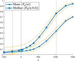
(a) Median returns

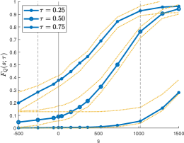
(b) Returns for $\tau=0.25,0.50,0.75$

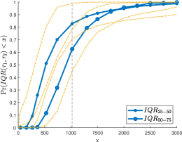
(c) IQR

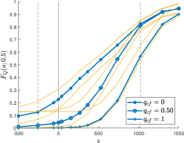
(d) Median Returns for $\boldsymbol{z}_{\text{cf}}=0,0.50,1$

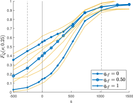
(e) Returns for $\tau=0.25$ and $\boldsymbol{z}_{\text{cf}}=0,0.50,1$

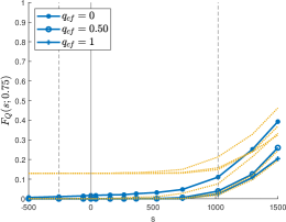
(f) Returns for $\tau=0.75$ and $\boldsymbol{z}_{\text{cf}}=0,0.50,1$

Figure 2(f), panel (a), illustrates the CDF $F_{Q}(s;0.5)$, the distribution of median ex ante returns at current beliefs $q_{i}$, and compares it to the estimated distribution of mean returns $F_{\mu}(s)$. $s$ is measured in monthly equivalent and varies on the x-axis between -500 and 1,500 EUR. Values estimated for $s$ below -250 EUR and above 1,100, marked with a dashed vertical lined, are typically outside the observed support of $B$, and therefore rely on extrapolating the conditional CDFs at larger values of $s$. The solid middle line represents the estimated distribution based on the point-identified procedure, whereas the lower and upper dotted lines represent the bound procedure (with $c=0.05$ in Equation (C.9)). Accounting for measurement errors through bounds makes it more difficult to identify the tails of the distribution for the median returns. However, the central part of the distribution is relatively well estimated.

The insights derived from the distribution of median and mean are somewhat different. The perceived median returns are essentially positive, with between 82 and 94 percent of the population exhibiting positive returns on overstaying. About half of the population perceives median return larger than 730 EUR. At least 22 percent perceive returns larger than 1,000 EUR per month. Thus, the distribution of median ex ante returns is very heterogeneous, with non-negligible portions of the population perceiving either negative or very large median returns. In contrast, the distribution of mean returns is shifted to the right with a support that is essentially positive and a median above 1,000 EUR. The discrepancy between mean and median returns suggests the existence and influence of large perceived returns.

Figure 2(f), panel (b), compares the distribution of median returns to the distribution of returns for additional quantiles, that is $F_{Q}(s;\tau)$ for $\tau=0.25$ (left/top distribution) and $\tau=0.75$ (right/bottom). For the distribution of first quartiles, between 32 and 41 percent of the population perceives negative ex ante returns, and the median stands between 140 and 330 EUR. For the distribution of third quartiles, the returns are essentially positive and very large. The lower bound seems conservative. Compared to the distribution $F_{Q}(s;0.25)$, $F_{Q}(s;0.75)$ is farther away from the distribution of median returns, $F_{Q}(s;0.5)$, implying that the individual-specific distributions of ex ante returns have a long upper tail.

The last point is best illustrated by the distribution of $IQR_{25-50}$ and $IQR_{50-75}$ in Figure 2(f), panel (c). These CDFs represent the proportion of the population for which the spread of the distributions of ex ante returns is below a given value. The distribution of $IQR_{50-75}$ is shifted to the right compared to the distribution of $IQR_{25-50}$. However, the latter results rely very much on the quality of our extrapolation. Notwithstanding this caveat, these findings suggest that usual assumptions on the resolvable uncertainty (independence with observed beliefs, separability, extreme-value type I representation and/or identical distribution) may not fit the data very well. Indeed, assuming that the resolvable uncertainty is separable, the long upper tail speaks against a symmetric distribution. Furthermore, the distribution of IQR does not seem to be degenerated, hinting to some variability of individuals’ perception of uncertainty.

The descriptive results in Section 6.2 highlighted the importance of the chance of becoming regularised for the decision to overstay. To emphasise this finding, Figure 2(f), panel (d), illustrates the CDF $\Pr\bigl{(}{Q_{S}\left({\tau;B,\boldsymbol{z}_{\text{cf}},\eta}\right)\leq s}\bigr{)}$, the distribution of median ex ante returns at counterfactuals values of $\boldsymbol{z}_{\text{cf}}$: $\boldsymbol{z}_{\text{cf}}=0$, left/top, $\boldsymbol{z}_{\text{cf}}=0.5$, middle, $\boldsymbol{z}_{\text{cf}}=1$, right/bottom. If there would be no chance of becoming regularised, the median returns would be negative for 15 to 30 percent of the population, and the median in this distribution would stand between 350 and 570 EUR. The distribution moves significantly to the right as the perceived chance of regularisation increases, with virtually everyone perceiving positive median returns on overstaying in the most optimistic scenario.

Finally, in Figure 2(f), panels (e) and (f) highlight the changing interaction between returns and chance of becoming regularised at different quantiles. Whereas at the first-quartile (panel (e), $\tau=0.25$) the chance of becoming regularised appears instrumental to shift returns into positive values, it has no such effect at the top-quartile (panel (f), $\tau=0.75$).

6.4. Policy Implications

This section illustrates two points: (1) the added information on the distribution of returns at different quantiles is key to derive accurate answers to meaningful policy questions; (2) the findings on Afghan asylum seekers’ perceived returns should inform the design of European migration policies.

Both points will be illustrated using the example of assisted voluntary return policies (VRPs). VRPs transfer cash to asylum seekers with a rejected application when they willingly return to their home country. Faced with high costs and administrative difficulties of forced returns, the European Commission and several members States have promoted voluntary returns as a “cost-effective” strategy to address the issue of overstay, a standpoint illustrated by the following statement of the Commissioner for Home Affairs: “Voluntary returns are always the better option: they put the individual at the core, they are more effective and less costly.”

A VRP is ‘effective’ if the level of (cash) transfers matches the ex ante perceived returns on overstaying of the marginal individual whose departure the government wishes to incentivise, making him or her indifferent to leaving or overstaying. The higher the perceived returns for this marginal individual, the more generous, i.e. costly, an effective policy will need to be. Perhaps less appreciated, the cost of a VRP also depends on the ex ante perceived returns for the inframarginal population: because VRPs are usually non-discriminating, the transfer received by inframarginal leavers may exceed their returns. In the extreme case where these returns are negative, VRPs may transfer funds to individuals who would have required no transfer to eventually leave the country.

The estimated distributions of perceived returns shed new light on the potential cost of VRPs, if we interpret these returns as a lower bound of the necessary transfer to induce return to the home country. Besides, observing the distribution of quantiles allows a richer analysis than would be permitted by observing just the distribution of median or mean returns. In fact, a focus on a single quantile can be quite misleading.

To understand the last point, it is important to take the perspective of a policy maker. From this perspective, the resolution of uncertainty will generate a mixture of shocks $\nu$ in the population. For some individuals, the realised uncertainty $\nu$ will correspond to lower quantiles $\tau$, whereas for others, it will correspond to higher quantiles $\tau$. Thus, if preferences and observed beliefs are stable, the realised distribution of returns will be a mixture of the ex ante distribution of quantiles $F_{Q}(s;\tau)$. If the policy maker considers that all asylum seekers have equally valid prior on the distribution of $\nu$ and shocks are i.i.d., the best predictor for the realised distribution of returns is a mixture of the distributions of quantiles with equal weights; that is:

$$\overline{F}_{S}(s):=\int_{0}^{1}F_{Q}(s;\tau)\omega_{\tau}d\tau$$ (6.1)

where $\omega_{\tau}=1$ for all $\tau$.

Instead, the policy maker may entertain a different prior: for example, if individuals are deemed to be too optimistic about the resolvable uncertainty, realised shocks would be overwhelmingly concentrated on the lowest quantiles. Thus, a policy maker may wish to assign low weights to the highest quantiles. If instead, individuals are assumed to place too much weight on extreme quantiles, the policy maker can discount extreme quantiles. A policy maker who bases their analysis solely on the distribution of median returns assigns a weight one to the median and zero to all other quantiles.

Taking the estimate of the distribution $F_{Q}(s;\tau),\tau\in(0,1)$ as a starting point, we can compare the insights from different weighting choices.

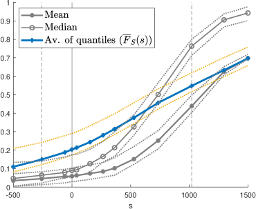
Figure 6.2. $\overline{F}_{S}(s)$ with equal weighting - compared to $F_{Q}(s;0.5)$ and $F_{\mu}(s)$

Figure 6.2 compares the distribution $\overline{F}_{S}(s)$ resulting from an equal weighting to the distributions of the median and the mean returns. Compared to the distribution of medians, the former distribution is substantially flatter, since it accounts for the fact that some people will see their upper quantiles realised, and these upper quantiles are significantly skewed toward high returns. Compared to the distribution of means, it suggests a higher probability of low returns, as it accounts for the fact that some people will see their lower quantiles realised, and these quantiles tend to represent low and negative returns. Hence, a focus on the median or the mean may be quite misleading.

The distribution $\overline{F}_{S}(s)$ is a useful tool to understand the effect of a cash transfer to asylum seekers. Such a transfer is easy to analyse since it shifts the distribution of returns to the left by a mere translation. To induce the departure of one quarter of asylum seekers, a VRP should transfer at least 10,750 EUR in Net Present Value (NPV). This number rises to 54,060 EUR for moving up to half of the population. A one-off cash transfer of the level implemented in Germany in 2017 (2,000 EUR $\approx$ 32.2 EUR/month for 72 months in NPV) would increase the departure rate by 0.8 percentage points (pp) from a baseline level of 20.4 percent. However because of the inframarginal individuals who would have needed no incentives to leave and may cash in the transfer, each additional leaver may cost up to 26.6 times the cash transfer they actually receive. This cost represents about 15.6 times the estimated average cost of a forced return, as estimated by the European Parliamentary Research Service.

Figure 6.3. $\overline{F}_{S}(s)$ with different weighting schemes.

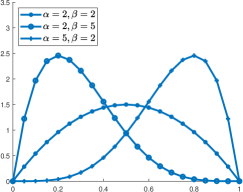
(a) Equal weighting

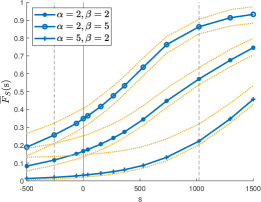
(b) Weighting through a beta-distribution

Figure 4(b), panel (b), compares the estimated distribution $\overline{F}_{S}(s)$ for different weighting schemes from a beta-distribution (illustrated in panel (a)). The first scheme weights the left and right tail quantiles down, and produces similar results as a uniform weighting. The second scheme weights only the upper quantiles down, and the third only the lower quantiles.

The distribution of returns moves to the left as more weights is put on lower quantiles. In this case which seems the most favourable for a VRP (i.e., requires lower transfer to reach the median), 34.9 percent leaves the country without requiring a transfer. The transfer should be at least 19,000 EUR for moving up to half of the population. A one-off cash transfer of 2,000 EUR would increase the departure rate by 1.27 percentage points (pp). However, if all leavers would cash in the VRP transfer, each additional leaver costs up to 28 times the cash transfer they actually receive.

Notwithstanding the specificity of Afghan asylum seekers and the limitations of the present analysis, these results put into perspective the argument of cost-effectiveness of VRPs. Unless they are large, transfers have little effect on overstay decisions, and may be more expensive than they appear at first sight.

7. Conclusion and Directions for Future Work

The general context of the paper is one in which individuals make a discrete human capital investment choice in an environment characterised by uncertainty about their future outcomes, with some but not all uncertainty being resolved over time. In this context, individuals form subjective expectations about their outcomes and the nature of uncertainty.

The paper demonstrates the usefulness of the stated preference approach to uncover population distributions of quantiles and means of ex ante returns, as well as quantile effects and mean effects of choice characteristics. In the case where perceived returns and resolvable uncertainty are additively separable, it also quantifies the amount of resolvable uncertainty perceived by the agent. The paper proposes identification results that build on the elicitation of both actual beliefs and intentions, and beliefs and intentions in a limited number of counterfactual scenarios. Thus, it takes full advantage of the flexibility available to the researcher when designing an elicitation procedure.

Comparing ex ante returns over time and against actual choices will be the natural continuation of this research agenda. For these endeavours, the characterisation of individuals’ resolvable uncertainty in this paper will undoubtedly be a strong asset. For example, once uncertainty is resolved and decision made, the population distribution of outcomes can be seen as reflecting an unobserved mixture of individuals’ resolved uncertainty. The results in the present paper identify the single components of this mixture. The analyst will then be able to make inference of the weights of the mixture and assess potential biases in the population.

In the ideal case, the researcher can design one or several scenarios common to all individuals. An alternative approach, not yet exploited by the literature is the control function approach in nonlinear models. Provided, the existence of an instrument affecting observed beliefs only, one could instead apply results on the estimation of nonseparable models (e.g. Imbens and Newey,, 2009; Chernozhukov and Hansen,, 2005). The exogenous instruments could be provided by the experimental variations of beliefs. This will be the focus of future research.

Other potential applications of the framework developed here include educational and occupational choices, retirement or economic migration decisions. It could also be applied to the estimation of a willingness to pay for a good as in Maestas et al., (2018), or to extend results on welfare analysis in discrete choice models, such as Bhattacharya, (2015, 2018), by using a stated choice analysis.

Appendix

Appendix A Additional Results

This section presents additional results of characterisation and identification. More specifically, Section A.1 introduces characterisation results for additional parameters of interest: mean ex ante returns, quantile effects, mean effects, and IQR. Section A.2 presents results for the case where $\boldsymbol{\eta}$ is multidimensional. Both types of results are single out in this section as they require additional notations.

A.1. Characterisation of parameter of interests

Start with two remarks:

Remark 2.

A result similar to Lemma 1 applies to the non-pecuniary disutility $C$. Under the assumptions of Lemma 1:

$$\Pr\left({C\leq c|\boldsymbol{\eta}}\right)=m(Y_{0}-c,c,\boldsymbol{Z},\boldsymbol{\eta})$$ (A.1)

Thus, the distribution of $C$ can be characterised in the population by results similar to Theorem 1.

Remark 3.

Given knowledge of the distribution of $S(\boldsymbol{x},\boldsymbol{\eta},\nu)$, one can derive the first moment, say $\mu_{S}(\boldsymbol{x},\boldsymbol{\eta})$ as in Chernozhukov et al., (2020) (cf. Karr,, 1993, pp. 113-114). Let $\mathcal{S}$ denote the support of $S$, and assume that $\mu_{S}$ is bounded. Then:

$$\mu_{S}(\boldsymbol{x},\boldsymbol{\eta})=\int_{\mathcal{S}^{+}}\left[{m(t(s,\boldsymbol{x}),\boldsymbol{\eta})}\right]ds-\int_{\mathcal{S}^{-}}\left[{1-m(t(s,\boldsymbol{x}),\boldsymbol{\eta})}\right]ds$$

To characterise the remaining objects of interest, the paper introduces a reduced form representation that is useful representation of the intended choice:

$$\begin{array}[]{l}P:=P_{\boldsymbol{X}}\text{ where }P_{\boldsymbol{x}}=h\left({\boldsymbol{x},\alpha_{\boldsymbol{x}}}\right)\text{ and }\alpha_{\boldsymbol{x}}\sim F_{\alpha}\end{array}$$ (A.2)

where $F_{\alpha}$ is a given CDF. Such representation always exists. For example, if $\alpha_{\boldsymbol{x}}\sim U(0,1)$ in equation (A.2), $h\left({\boldsymbol{x},\alpha_{\boldsymbol{x}}}\right)$ is the $\alpha_{\boldsymbol{x}}$-quantile of the random variable $P_{\boldsymbol{x}}$ (see, for example, the Skohorod representation of Chernozhukov and Hansen, (2005)). In general, the collection of variables $\{\alpha_{\boldsymbol{x}}\}$ is not independent of $\boldsymbol{X}$. The interest of this representation is the dimension reduction from the multidimensional random vector $\boldsymbol{\eta}$ to the real random variable $\alpha_{\boldsymbol{X}}$. This representation facilitates the characterisation for the remaining distributions of interest contained in Theorem 3 below. The characterisation in Theorem 1 can be rewritten as in Corollary 1.

Corollary 1.

Under Assumption 1 and Assumption 2, the following holds for any real value $s$ and and $p\in[0,1]$:

$$F_{Q}(s;\tau)=\int_{\mathcal{X}}\int_{0}^{1}1\left\{{h\left({t(s,\boldsymbol{x}),Q_{\alpha_{t(s,\boldsymbol{X})}|\boldsymbol{X}}\left({a|\boldsymbol{x}}\right)}\right)\leq 1-\tau}\right\}da\;dF_{\boldsymbol{X}}(\boldsymbol{x})$$

where $t(s,\boldsymbol{x}):=(y_{0}+s,b-s,\boldsymbol{z})$.

Theorem 3 provides a characterisation for the remaining distributions of interest.

Theorem 3.

Recall that $\mathcal{S}$ denotes the support of $S$. Under the conditions of Theorem 1 and for $\mu_{S}$ bounded, the population distributions of interest are characterised as follows: Define

$$\begin{array}[]{l}A^{+}(\boldsymbol{x},a)=\int_{\mathcal{S}^{+}}\left[{m(t(s,\boldsymbol{x}),Q_{\alpha_{t(s,\boldsymbol{x})}|\boldsymbol{X}}(a|\boldsymbol{x}))}\right]ds,\\ A^{-}(\boldsymbol{x},a)=\int_{\mathcal{S}^{-}}\left[{1-m(t(s,\boldsymbol{x}),Q_{\alpha_{t(s,\boldsymbol{x})}|\boldsymbol{X}}(a|\boldsymbol{x}))}\right]ds,\\ \mu_{A}(\boldsymbol{x},a)=A^{+}(\boldsymbol{x},a)-A^{-}(\boldsymbol{x},a)\\ A^{\tau}(\boldsymbol{x},a)=\int_{\mathcal{S}}1\{s\geq 0\}-1\left\{{\left[{1-m(t(s,\boldsymbol{x}),Q_{\alpha_{t(s,\boldsymbol{x})}|\boldsymbol{X}}(a|\boldsymbol{x}))}\right]\geq\tau}\right\}ds,\end{array}$$

$\text{ where }\mathcal{S}^{+}=\mathbb{R}^{+}\cap\mathcal{S}\text{ and }\mathcal{S}^{-}=\mathbb{R}^{-}\cap\mathcal{S}$. Then, we have:

$$\Pr\left({\mu_{S}(\boldsymbol{X},\boldsymbol{\eta})\leq y}\right)=\int_{\mathcal{X}}\int_{0}^{1}1\left\{{\mu_{A}(\boldsymbol{x},a)\leq y}\right\}da\;dF_{\boldsymbol{X}}(\boldsymbol{x}),$$

$$\Pr\left({QE_{j,h}(\tau;\boldsymbol{X},\boldsymbol{\eta})\leq y}\right)=\int_{\mathcal{X}}\int_{0}^{1}1\left\{{A^{\tau}(\boldsymbol{x}+h\boldsymbol{e}_{j},a)-A^{\tau}(\boldsymbol{x},a)\leq y}\right\}da\;dF_{\boldsymbol{X}}(\boldsymbol{x}),$$

$$\Pr\left({ME_{j,h}(\boldsymbol{X},\boldsymbol{\eta})\leq y}\right)=\int_{\mathcal{X}}\int_{0}^{1}1\left\{{\mu_{A}(\boldsymbol{x}+h\boldsymbol{e}_{j},a)-\mu_{A}(\boldsymbol{x},a)\leq y}\right\}da\;dF_{\boldsymbol{X}}(\boldsymbol{x}),$$

$$\Pr\left({IQR(\boldsymbol{X},\boldsymbol{\eta};\tau_{1},\tau_{2})\leq y}\right)=\int_{\mathcal{X}}\int_{0}^{1}1\left\{{A^{\tau_{2}}(\boldsymbol{x},a)-A^{\tau_{1}}(\boldsymbol{x},a)\leq y}\right\}da\;dF_{\boldsymbol{X}}(\boldsymbol{x}).$$

As with Theorem 1, Theorem 3 implies that identification of the function $h(\boldsymbol{x},\alpha_{\boldsymbol{x}})$ and the conditional distribution of $\alpha_{\boldsymbol{x}}$ is sufficient for identification of the distributions of interest.

A.2. Identification results for a multidimensional $\boldsymbol{\eta}$

This section first updates Assumption 4 to consider a multidimensional $\boldsymbol{\eta}$, and the associated reduced form in Equation (A.2) (Section A.2.1). Then, it reinterprets the assumption of a univariate variate heterogeneity as a special case of Rank Invariance (Section A.2.2). Finally, it shows identification under the assumption of a random coefficient model for the quantiles of the reduced form (Section A.2.3). In this case, additional counterfactual scenarios can be harnessed to relax restrictions on the dimension of $\boldsymbol{\eta}$.

A.2.1. Data

Using notations from Section A.1, Assumption 6 summarises the structure of the data available to the researcher.

Assumption 6 (Pseudo-panel).

Let $t=0$ denote the actual scenario, and $t=1,\ldots,T,$ be the index for $T$ hypothetical scenarios. The researcher observes an i.i.d. sample, $\{P_{it},\boldsymbol{X}_{it}:i=1,\ldots,N;t=0,1,\ldots,T\}$ such that:

$$\begin{array}[]{l}P_{it}=h(\boldsymbol{X}_{it},\alpha_{it}+\epsilon_{it}),\text{ for all }i\text{ and }t=0,1,\ldots,T\end{array}$$ (A.3)

where $\alpha_{it}:=\alpha_{\boldsymbol{X}_{it}}$:

1. for any $a\in[0,1]$, $h(\boldsymbol{x},Q_{\alpha_{\boldsymbol{x}}}(a))=Q_{\Pi_{it}|\boldsymbol{X}_{it}}(a|\boldsymbol{x}),i=1,\ldots,N,t=0,1,\ldots,T$,

2. $\epsilon_{it}$ is a continuously distributed random variable capturing a measurement error.

In particular, among the $T$ counterfactual scenarios, $T_{1}$ are common to all respondents $i$:

1. there exists $\bar{\boldsymbol{x}_{t}}=(\bar{y}_{t},\bar{b}_{t},\bar{\boldsymbol{z}}_{t}),\;t=1,2,\ldots,T_{1}$, with $T_{1}\leq T$ such that $\boldsymbol{X}_{it}=\bar{\boldsymbol{x}}_{t}$,

As before, $P_{i0}$ denotes the stated actual choice probability, $\boldsymbol{X}_{i0}$ the vector of observed beliefs held, $P_{it},t=1,\ldots,T$ the stated probabilistic choices in counterfactual scenarios, and $\boldsymbol{X}_{it},t=1,\ldots,T,$ the beliefs held in counterfactual scenarios.

Conditions (i) states that the data are represented by a reduced form function related to the quantile structural function, up to a normalisation. The reported intentions $\{P_{it}:t=0,1,\ldots,T\}$ deviate from the true intentions, $\{\Pi_{it}:t=0,1,\ldots,T\}$, because of a measurement error summarised by the random variable $\epsilon_{it}$. Condition $(CF)$ states that the intended choices are observed at some counterfactual values $\{\bar{\boldsymbol{x}}_{t}:t=1,\ldots,T_{1}\}$ and these hypothetical scenarios provide a complete description of observed beliefs.

A.2.2. Identification with Rank Invariance/Similarity

The identification result derived in the main text, Theorem 2, corresponds to the case of either Rank Invariance or Rank Similarity. Rank Invariance applies to the leading case when $\boldsymbol{\eta}$ is univariate and can be treated as a nonseparable individual fixed effect. Rank similarity applies when $\boldsymbol{X}$ is independent of $\boldsymbol{\eta}$, for example, when beliefs are elicited at experimentally set values. In each case, only $T=1$ is necessary to recover the objects of interest.

The next assumption makes explicit the restriction on the rank variable $\{\alpha_{it}:{t=0,1,\ldots,T}\}$ that allows identification when $T=1$.

Assumption 7 (Rank Invariance/Rank Similarity).

With the notations of Assumption 4, either:

• $\left\{{\alpha_{it}:t=0,\ldots,T}\right\}$ are equal to each other,

• or the conditional distribution of $\left\{{\alpha_{it}:t=0,\ldots,T}\right\}$ (conditonal on $\boldsymbol{X}$) are equal to each other.

Condition $(RI)$ imposes a rank invariance on $\Pi_{it}$ with respect to $\boldsymbol{X}_{it}$. Rank Invariance has been introduced by Doksum, (1974) and used more recently by Heckman et al., (1997), Chernozhukov and Hansen, (2005), and Torgovitsky, (2015) among others. Under $(RI)$, $\alpha_{it}$ becomes an individual fixed effect, $\alpha_{i}$.

Condition $(RS)$ is a slightly weaker alternative to $(RI)$ introduced by Chernozhukov and Hansen, (2005). In cases where beliefs are elicited at values that are generated randomly $\;\alpha_{it}$ is independent of $\boldsymbol{X}$ and can be normalised, for example, to follow a uniform distribution.

Under Assumption 7 and with appropriate modifications to Assumption 5 (replacing $m(\boldsymbol{x},\cdot)$ with $h(\boldsymbol{x},\cdot)$), Theorem 2 ensures identification of the parameters of interest from the joint distribution of available data.

A.2.3. Relaxing Rank Invariance/Similarity

Condition (RI) is a strong condition as discussed, for example, by Torgovitsky, (2015). Theorem 4 shows that additional counterfactual scenarios may also serve to relax the stringent condition (RI).

Theorem 4.

Suppose Assumptions 1, 2, 3, 5 (with appropriate modifications), and 6 all hold. In addition, the following conditions hold:

• there exist a known vector-valued function $\boldsymbol{x}\mapsto\boldsymbol{R}(\boldsymbol{x})$ and a random vector $\boldsymbol{A}$ both of dimension $d$, such that:

  $$\alpha_{\boldsymbol{X}}=\sum_{j=1}^{d}A_{j}R_{j}(\boldsymbol{X})=\boldsymbol{A}\cdot\boldsymbol{R}(\boldsymbol{X})^{\prime}$$ (A.4)

• Denote by $\boldsymbol{W}:=[R(\bar{\boldsymbol{x}}_{1}),\ldots,R(\bar{\boldsymbol{x}}_{T})]^{\prime}$. The matrix $\boldsymbol{W}^{\prime}\boldsymbol{W}$ is invertible.

• For $T$ i.i.d. draws of measurement errors: $\boldsymbol{\epsilon}=(\epsilon_{1},\ldots,\epsilon_{T})^{\prime}$, the characteristic function of $\boldsymbol{R}(\boldsymbol{X})(\boldsymbol{W}^{\prime}\boldsymbol{W})^{-1}\boldsymbol{W}^{\prime}\boldsymbol{\epsilon}$ is non vanishing.

• for all $a\in(\underline{\tau}(\boldsymbol{x}),\overline{\tau}(\boldsymbol{x}))$, we have $h(\bar{\boldsymbol{x}}_{t},a)=a$, $t=1,\ldots,T$.

Then, the distribution of returns as characterised in Theorem 1 and the other objects of interest in Theorem 3 are identified from the joint distribution of $(P_{0},\boldsymbol{X}_{0},P_{1},\boldsymbol{X}_{1},\ldots,P_{T},\boldsymbol{X}_{T})$.

For example, in the case of negligible measurement error, $P_{t}=\Pi_{t}$, for all $t=0,1,\ldots,T$, we have:

$$F_{Q}(s;\tau)=\mathbb{E}\left[{1\left\{{F_{\tilde{P}|\boldsymbol{X}_{0}}(\tilde{P}|t(s,\boldsymbol{X}))\leq F_{\pi_{0}|\boldsymbol{X}_{0}}\left({1-\tau|t(s,\boldsymbol{X})}\right)}\right\}}\right]$$ (A.5)

where $\tilde{P}=\boldsymbol{R}(t(s,\boldsymbol{X}))(\boldsymbol{W}^{\prime}\boldsymbol{W})^{-1}\boldsymbol{W}^{\prime}\left({P_{1},\ldots,P_{T}}\right)^{\prime}$.

Theorem 4 introduces a relaxation of conditions (RI) and (RS). Heuristically, Condition (RI) imposes that individuals do not ‘switch ranks’ as $\boldsymbol{X}$ varies, while Condition (RS) permits rank switching, which are independent of $\boldsymbol{X}$. Under Condition (RI) or (RS), Theorem 2 delivers identification because the elicitation of intentions in a common scenario ($P_{1}$) allows to rank individuals (or obtain the distribution of rankings). When those conditions fail, the random coefficient representation of Equation (A.4) allows rank switching that depends on $\boldsymbol{X}$. For example, with this assumption, when the unobserved heterogeneity, $\boldsymbol{\eta}$, is two-dimensional, there exists a pair $(\epsilon_{i1},\epsilon_{i2})$, such that for each individual, $\alpha_{\boldsymbol{X}_{i}}=\epsilon_{i1}+X_{i1}\epsilon_{i2}$, with $X_{i1}$ a subvector of $\boldsymbol{X}_{i}$. In this case, two hypothetical, linearly independent, and common scenarios are enough. When $\boldsymbol{\eta}$ is three-dimensional, three scenarios are necessary, and so forth. Hence, with enough counterfactual scenarios -Condition (CF’)-, one can trace out a ‘pattern’ of rank switching, using a linear combination of the stated intentions in hypothetical scenarios $(P_{1},\ldots,P_{T})$ and control for endogeneity.

Appendix B Proofs

B.1. Proof of Lemma 1

First, extend the definition of the map: $(s,\boldsymbol{x},\boldsymbol{\eta})\mapsto m(t(s,\boldsymbol{x}),\boldsymbol{\eta})$.

$$m(t(s,\boldsymbol{x}),\boldsymbol{\eta})=\left\{{\begin{array}[]{l}1\text{ if }s\leq\underline{s}(\boldsymbol{x},\boldsymbol{\eta})\\ 0\text{ if }s\geq\overline{s}(\boldsymbol{x},\boldsymbol{\eta})\\ \int 1\left\{{U_{1}(Y_{0}+B,\boldsymbol{Z}_{1},\boldsymbol{\eta}_{i},u)\geq U_{0}(Y_{0},\boldsymbol{Z}_{0},\boldsymbol{\eta},u)}\right\}dF_{\nu|\boldsymbol{X},\boldsymbol{\eta}}\left({u|t(s,\boldsymbol{x}),\boldsymbol{\eta}}\right)\text{, otherwise}\end{array}}\right.$$

The map is well defined by Assumption 3, since $t(s,\boldsymbol{x})\in\mathcal{X}$, for $s\in\bigl{[}{\underline{s}(\boldsymbol{x},\boldsymbol{\eta});\overline{s}(\boldsymbol{x},\boldsymbol{\eta})}\bigr{]}$.

By Assumption 3, for $s\leq\underline{s}(\boldsymbol{x},\boldsymbol{\eta})$, $\Pr\bigl{[}{S(\boldsymbol{x},\boldsymbol{\eta},\nu)\leq s|\boldsymbol{\eta}}\bigr{]}=1-m\left({t(s,\boldsymbol{x}),\boldsymbol{\eta}}\right)=0$. Similarly: $s\geq\overline{s}(\boldsymbol{x},\boldsymbol{\eta})$, $\Pr\bigl{[}{S(\boldsymbol{x},\boldsymbol{\eta},\nu)\leq s|\boldsymbol{\eta}}\bigr{]}=1-m\left({t(s,\boldsymbol{x}),\boldsymbol{\eta}}\right)=1$. Consider $s\in\bigl{[}{\underline{s}(\boldsymbol{x},\boldsymbol{\eta});\overline{s}(\boldsymbol{x},\boldsymbol{\eta})}\bigr{]}$. By Equation (4.1), we have:

$$\begin{array}[]{l}\Pr\bigl{[}{S(\boldsymbol{x},\boldsymbol{\eta},\nu)\leq s|\boldsymbol{\eta}}\bigr{]}\\ =\Pr\bigl{[}{U_{0}^{-1}\left({U_{1}\left({y_{0}+b,\boldsymbol{z}_{1},\boldsymbol{\eta},\nu}\right),\boldsymbol{z}_{0},\boldsymbol{\eta},\nu)}\right)-y_{0}\leq s|\boldsymbol{\eta}}\bigr{]}\\ =\Pr\bigl{[}{U_{1}(y_{0}+b,\boldsymbol{z}_{1},\boldsymbol{\eta},\nu)\leq U_{0}(y_{0}+s,\boldsymbol{z}_{0},\boldsymbol{\eta},\nu)|\boldsymbol{\eta}}\bigr{]}\\ =\Pr\bigl{[}{U_{1}((y_{0}+s)+(b-s),\boldsymbol{z}_{1},\boldsymbol{\eta},\nu)\leq U_{0}(y_{0}+s,\boldsymbol{z}_{0},\boldsymbol{\eta},\nu)|\boldsymbol{\eta}}\bigr{]}\\ =_{(1)}\Pr\bigl{[}{U_{1}(Y_{0}+B,\boldsymbol{Z}_{1},\boldsymbol{\eta},\nu)\leq U_{0}(Y_{0},\boldsymbol{Z}_{0},\boldsymbol{\eta},\nu)|Y_{0}=y_{0}+s,B=b-s,\left({\boldsymbol{Z}_{0},\boldsymbol{Z}_{1}}\right)=\left({\boldsymbol{z}_{0},\boldsymbol{z}_{1}}\right),\boldsymbol{\eta}}\bigr{]}\\ =1-m\left({y_{0}+s,b-s,\boldsymbol{z},\boldsymbol{\eta}}\right)\\ =1-m\left({t(s,\boldsymbol{x}),\boldsymbol{\eta}}\right)\end{array}$$

where equality (1) uses Assumption 2.

B.2. Proof of Theorem 1

The second equality follows from Lemma 1 and integrating Equation (4.4) with respect to the joint distribution of $(\boldsymbol{X},\boldsymbol{\eta})$.

To arrive at the first equality, note first that by definition of $Q_{S}(\tau;\boldsymbol{x},\eta)$ and Lemma 1, for any $\tau\in(0,1)$ :

$$\Pr\left({S\left({\boldsymbol{x},\boldsymbol{\eta},\nu}\right)\leq Q_{S}(\tau;\boldsymbol{x},\eta)|\boldsymbol{\eta}}\right)=1-m\left({t\bigl{(}{Q_{S}(\tau;\boldsymbol{x},\eta),\boldsymbol{x}}\bigr{)},\boldsymbol{\eta}}\right)\geq\tau.$$

The next lines show that the events $\left\{Q_{S}(\tau;\boldsymbol{x},\eta)\leq s\right\}$ and $\left\{{m\left({t(s,\boldsymbol{x}),\boldsymbol{\eta}}\right)\leq 1-\tau}\right\}$ are equal almost surely. For some $s$:

$$Q_{S}(\tau;\boldsymbol{x},\eta)\leq s \Rightarrow m\left({t(s,\boldsymbol{x}),\boldsymbol{\eta}}\right)\leq m\left({t\bigl{(}{Q_{S}(\tau;\boldsymbol{x},\eta),\boldsymbol{x}}\bigr{)},\boldsymbol{\eta}}\right)$$

$$\Rightarrow m\left({t(s,\boldsymbol{x}),\boldsymbol{\eta}}\right)\leq 1-\tau$$

where the first implication comes from the monotonicity of $m$: with greater transfers $s$, the intention to choose sector 1 decreases. Similarly, for some $s$ :

$$m\left({t(s,\boldsymbol{x}),\boldsymbol{\eta}}\right)\leq 1-\tau \Rightarrow 1-m\left({t(s,\boldsymbol{x}),\boldsymbol{\eta}}\right)\geq\tau$$

$$\Rightarrow \Pr\left({S(\boldsymbol{x},\boldsymbol{\eta},\nu)\leq s|\boldsymbol{\eta}}\right)\geq\tau$$

$$\Rightarrow Q_{S}(\tau;\boldsymbol{x},\boldsymbol{\eta})\leq s$$

B.3. Proof of Theorem 2

To prove the result, we need to prove that the structural quantile function and the conditional distribution of the rank variable are both identified. Note that by Assumption 4.(i)-(ii), it suffices to identify $m$ and the distribution of $\eta$.

First, note the normalisation of Assumption 5.$(QF).(ii)$ implies that the following conditional distribution is identified from the data:

$$F_{\eta+\epsilon_{1}|\boldsymbol{X}_{t},\boldsymbol{X}_{1}}(a|\boldsymbol{x},\bar{\boldsymbol{x}})=F_{P_{1}|\boldsymbol{X}_{t},\boldsymbol{X}_{1}}(a|\boldsymbol{x},\bar{\boldsymbol{x}})$$ (B.1)

Hence, for all $\boldsymbol{x}$ such that $(\boldsymbol{X}_{0},\boldsymbol{X}_{1})=(\boldsymbol{x},\bar{\boldsymbol{x}})$ and for all $a$ such that $\underline{\tau}(x)<a<\overline{\tau}(x)$:

$$\begin{array}[]{lll}Q_{P_{0}|\boldsymbol{X}_{0},\boldsymbol{X}_{1}}\left({F_{P_{1}|\boldsymbol{X}_{0},\boldsymbol{X}_{1}}(a|\boldsymbol{x},\bar{\boldsymbol{x}})|\boldsymbol{x},\bar{\boldsymbol{x}}}\right)&=_{(1)}&Q_{m(\boldsymbol{X}_{0},\eta+\epsilon_{0})|\boldsymbol{X}_{0},\boldsymbol{X}_{1}}\left({F_{P_{1}|\boldsymbol{X}_{0},\boldsymbol{X}_{1}}(a|\boldsymbol{x},\bar{\boldsymbol{x}})|\boldsymbol{x},\bar{\boldsymbol{x}}}\right)\\ &=_{(2)}&Q_{m(\boldsymbol{X}_{0},\eta+\epsilon_{0})|\boldsymbol{X}_{0},\boldsymbol{X}_{1}}\left({F_{\eta+\epsilon_{1}|\boldsymbol{X}_{0},\boldsymbol{X}_{1}}(a|\boldsymbol{x},\bar{\boldsymbol{x}})|\boldsymbol{x},\bar{\boldsymbol{x}}}\right)\\ &=_{(3)}&m\left({\boldsymbol{x},Q_{\eta+\epsilon_{0}|\boldsymbol{X}_{0},\boldsymbol{X}_{1}}\left({F_{\eta+\epsilon_{1}|\boldsymbol{X}_{0},\boldsymbol{X}_{1}}(a|\boldsymbol{x},\bar{\boldsymbol{x}})|\boldsymbol{x},\bar{\boldsymbol{x}}}\right)}\right)\\ &=_{(4)}&m(\boldsymbol{x},a).\end{array}$$ (B.2)

Equality (1) follows from Assumption 4, equality (2) from Equation (B.1), equality (3) from the monotonicity condition (QF), and equality (4) from Conditions (ME) in Assumption 4.

Note that $m(\boldsymbol{x},a)$ is identified for all $\boldsymbol{x}$, such that $(\boldsymbol{x},\bar{\boldsymbol{x}})$ belongs to the support of $(\boldsymbol{X}_{0},\boldsymbol{X}_{1})$, $\mathcal{X}_{0}\mathcal{X}_{1}:=\mathit{Supp}(X_{0},X_{1})$. Hence, identification of $h(\boldsymbol{x},a)$ depends on the richness of the support $\boldsymbol{X}_{0}$, for individuals such that $\boldsymbol{X}_{1}=\bar{\boldsymbol{x}}$. Condition (CF) of Assumption 4 ensures that this support is not restricted, because one counterfactual elicits intention $P_{1}$ at $\boldsymbol{X}_{1}=\bar{\boldsymbol{x}}$ for the entire sample. Hence, under (CF), $\{\boldsymbol{X}_{0}=\boldsymbol{x},\boldsymbol{X}_{1}=\bar{\boldsymbol{x}}\}=\{\boldsymbol{X}_{0}=\boldsymbol{x}\}$ and Equation (B.2) simplifies to

$$m(\boldsymbol{x},a)=Q_{P_{0}|\boldsymbol{X}_{0}}\left({F_{P_{1}|\boldsymbol{X}_{0}}(a|\boldsymbol{x})|\boldsymbol{x}}\right).$$

Consider now the identification of the conditional distribution of $\eta$. Note that for each $\boldsymbol{x}$:

$$\underline{\tau}(\boldsymbol{x}) = \inf\left\{{a:m(\boldsymbol{x},a)>0}\right\}$$ (B.3)

$$\overline{\tau}(\boldsymbol{x}) = \sup\left\{{a:m(\boldsymbol{x},a)<1}\right\}$$ (B.4)

Denote by $\underline{p}(\boldsymbol{x})=\Pr(\pi_{t}=0|\boldsymbol{X}_{t}=\boldsymbol{x})$ and $\overline{p}(\boldsymbol{x})=\Pr(\pi_{t}=1|X_{t}=x)$. For all $p\in(\underline{p}(x),1-\overline{p}(x))$:

$$Q_{P_{0}|X_{0}}(a|\boldsymbol{x})=Q_{m(\boldsymbol{X}_{t},\eta+\epsilon_{0})|X_{0}}(a|\boldsymbol{x})=m\left({\boldsymbol{x},Q_{\eta+\epsilon_{0}|\boldsymbol{X}_{0}}(a|\boldsymbol{x})}\right)$$

By the monotonicity condition 5.$(ii)$:

$$\left\{\begin{array}[]{lll}Q_{\eta+\epsilon_{0}|X_{t}}(a|\boldsymbol{x})&=&m^{-1}\left({\boldsymbol{x},Q_{P_{0}|\boldsymbol{X}_{0}}(a|\boldsymbol{\boldsymbol{x}})}\right)\text{ if }a\in(\underline{\tau}(\boldsymbol{x}),1-\overline{\tau}(\boldsymbol{x}))\\ Q_{\eta+\epsilon_{0}|X_{i}}(a|\boldsymbol{x})&\leq&\underline{\tau}(\boldsymbol{x})\text{ if }a\leq\underline{\tau}(\boldsymbol{x})\\ Q_{\eta+\epsilon_{0}|X_{i}}(a|\boldsymbol{x})&\geq&\overline{\tau}(\boldsymbol{x})\text{ if }a\geq 1-\overline{\tau}(\boldsymbol{x})\\ \end{array}\right.$$ (B.5)

Under Condition (CF) of Assumption 4, $(m)^{-1}\left({\boldsymbol{x},a}\right)=Q_{P_{1}|\boldsymbol{X}_{0}}\left({F_{P_{0}|\boldsymbol{X}_{0}}(a|\boldsymbol{x})|\boldsymbol{x}}\right)$ and $Q_{\eta+\epsilon_{0}|\boldsymbol{X}_{0}}(a|\boldsymbol{x})$ simplifies to $Q_{P_{1}|\boldsymbol{X}_{0}}(a|\boldsymbol{x})$.

The last step of the proof consists in a deconvolution of $\eta_{0}$ and $\epsilon_{0}$. The argument here is a direct application of Lemma 1 of Evdokimov, (2010). It uses the fact that $\bar{\boldsymbol{x}}$ represents the actual set of beliefs for some individuals in the population.

$$\begin{pmatrix}P_{0}\\ P_{1}\end{pmatrix} \bigg{\rvert}\left\{\boldsymbol{X}_{t}=\boldsymbol{X}_{1}=\bar{\boldsymbol{x}}\right\}=\begin{pmatrix}\eta+\epsilon_{0}\\ \eta+\epsilon_{1}\end{pmatrix}$$ (B.6)

By Condition (ME) and Lemma 1 of Evdokimov, (2010), the distribution of $\epsilon_{0}$ is identified. Therefore the characteristic function of $V$ is identified from the data. The conditional characteristic function of $\eta$ can then be written as:

$$\phi_{\eta}(s|\boldsymbol{X}_{0}=\boldsymbol{x})=\phi_{P_{0}}(s|\boldsymbol{X}_{0}=\boldsymbol{x})/\phi_{\epsilon}(s).$$ (B.7)

All terms on the right-hand side are identified from the data. Knowledge of the characteristic function being equivalent to the knowledge of the distribution function, this completes the proof of identification for the conditional distribution of the rank variable.

Suppose $P_{t}=\Pi_{t}$, for all $t=0,1,\ldots,T$. Under the conditions of Theorem 2, in particular condition (CF), $F_{\eta|\boldsymbol{X}_{0},\boldsymbol{X}_{1}}(a|\boldsymbol{x},\bar{\boldsymbol{x}})=F_{\eta|\boldsymbol{X}_{0}}(a|\boldsymbol{x})=F_{P_{1}|\boldsymbol{X}_{0}}$. Furthermore, Equation (B.2) implies that:

$$\begin{array}[]{ll}1\{m(t(s,\boldsymbol{x}),a)\geq 1-\tau\}&=1\left\{{Q_{P_{0}|\boldsymbol{X}_{0},\boldsymbol{X}_{1}}\left({F_{P_{1}|\boldsymbol{X}_{0},\boldsymbol{X}_{1}}(a|t(s,\boldsymbol{x}),\bar{\boldsymbol{x}})|t(s,\boldsymbol{x}),\bar{\boldsymbol{x}}}\right)\geq 1-\tau}\right\}\\ &=1\left\{{Q_{P_{0}|\boldsymbol{X}_{0}}\left({F_{P_{1}|\boldsymbol{X}_{0}}(a|t(s,\boldsymbol{x}))|t(s,\boldsymbol{x})}\right)\geq 1-\tau}\right\}\\ &=1\left\{{F_{P_{1}|\boldsymbol{X}_{0}}(a|t(s,\boldsymbol{x}))\geq F_{P_{0}|\boldsymbol{X}_{0}}\left({1-\tau|t(s,\boldsymbol{x})}\right)}\right\}\end{array}$$ (B.8)

where $t(s,\boldsymbol{x})=(y+s,b-s,\boldsymbol{z})$. Hence:

$$\begin{array}[]{l}\Pr\left[{\Pr\left({S(\boldsymbol{X},\eta,\nu)\leq s|\boldsymbol{\eta}}\right)\leq p}\right]\\ =1-\int\int_{0}^{1}1\left\{{m(t(s,\boldsymbol{x}),a)\geq 1-\tau}\right\}dF_{\eta|\boldsymbol{X}}(da|\boldsymbol{x})dF_{\boldsymbol{X}}(\boldsymbol{x})\\ =\int\int_{0}^{1}1\left\{{F_{P_{1}|\boldsymbol{X}_{0}}(a|t(s,\boldsymbol{x}))\geq F_{P_{0}|\boldsymbol{X}_{0}}\left({1-\tau|t(s,\boldsymbol{x})}\right)}\right\}dF_{\eta|\boldsymbol{X}}(a|\boldsymbol{x})dF_{\boldsymbol{X}}(\boldsymbol{x})\\ =\int\int_{0}^{1}1\left\{{F_{P_{1}|\boldsymbol{X}_{0}}(a|t(s,\boldsymbol{x}))\geq F_{P_{0}|\boldsymbol{X}_{0}}\left({1-\tau|t(s,\boldsymbol{x})}\right)}\right\}dF_{P_{1}|\boldsymbol{X}}(a|\boldsymbol{x})dF_{\boldsymbol{X}}(\boldsymbol{x})\\ =\mathbb{E}\left[{1\left\{{F_{P_{1}|\boldsymbol{X}_{0}}(P_{1}|t(s,\boldsymbol{X}))\geq F_{P_{0}|\boldsymbol{X}_{0}}\left({1-\tau|t(s,\boldsymbol{X})}\right)}\right\}}\right]\end{array}$$ (B.9)

The proof for the case covered by Theorem 4 follows mutatis mutandis.

B.4. Proof of Theorem 3

By Remark 3, the population distribution of $\mu_{S}(\boldsymbol{x},\boldsymbol{\eta})$ is obtained by integrating over $(\boldsymbol{x},\boldsymbol{\eta})$:

$$\begin{array}[]{l}\Pr\left({\mu_{S}(\boldsymbol{x},\boldsymbol{\eta})\leq y}\right)\\ =\int_{\mathcal{X}\times\mathcal{H}}\left\{{\int_{\mathcal{S}^{+}}\left[{m(t(s,\boldsymbol{x}),\boldsymbol{n})}\right]ds-\int_{\mathcal{S}^{-}}\left[{1-m(t(s,\boldsymbol{x}),\boldsymbol{n})}\right]ds\leq y}\right\}dF_{\boldsymbol{X},\boldsymbol{\eta}}(\boldsymbol{x},\boldsymbol{n})\\ =\int_{\mathcal{X}}\int_{0}^{1}\left\{{\int_{\mathcal{S}^{+}}\left[{h(t(s,\boldsymbol{x}),a)}\right]ds-\int_{\mathcal{S}^{-}}\left[{1-h(t(s,\boldsymbol{x}),a)}\right]ds\leq y}\right\}dF_{\alpha_{t(s,\boldsymbol{x})}|\boldsymbol{X}}(a|\boldsymbol{x})dF_{\boldsymbol{X}}(\boldsymbol{x})\\ =\int_{\mathcal{X}}\int_{0}^{1}\left\{{\int_{\mathcal{S}^{+}}\left[{h(t(s,\boldsymbol{x}),Q_{\alpha_{t(s,\boldsymbol{X})}|\boldsymbol{X}}(a|\boldsymbol{x}))}\right]ds}\right.\\ \;\;\;\;\;\;\;\;\;\;\;\;\;\;\;\;\;\;\;\;\;\;\;\;\;\;\;\;\;\;\;\;\left.{-\int_{\mathcal{S}^{-}}\left[{1-h(t(s,\boldsymbol{x}),Q_{\alpha_{t(s,\boldsymbol{x})}|\boldsymbol{X}}(a|\boldsymbol{x}))}\right]ds\leq y}\right\}da\;dF_{\boldsymbol{X}}(\boldsymbol{x})\end{array}$$ (B.10)

The proof is similar for the distribution of $ME$, $QE$, and $IQR$.

B.5. Proof of Corollary 1

Denote by $t(s,\boldsymbol{x}):=(y_{0}+s,b-s,q)$. The random variable $m(t(s,\boldsymbol{x}),\boldsymbol{\eta})$ can be represented by its quantile function $h(t(s,\boldsymbol{x}),\tau_{t(s,\boldsymbol{x})})$, with $\eta_{t(s,\boldsymbol{x})}\sim F_{\eta}$. Hence:

$$F_{Q}(s;\tau) = \int 1\left\{{m(t(s,\boldsymbol{x}),\boldsymbol{n})\geq 1-p}\right\}dF_{\boldsymbol{X},\boldsymbol{\eta}}(\boldsymbol{x},\boldsymbol{n})$$

$$=_{(1)} \int_{\mathcal{X}}\int_{0}^{1}1\left\{{Q_{m(t(s,\boldsymbol{X}),\boldsymbol{\eta})|\boldsymbol{X}}(a|\boldsymbol{x})\geq 1-\tau}\right\}dF_{\alpha_{t(s,\boldsymbol{x})}|\boldsymbol{X}}(a|\boldsymbol{x})\;dF_{\boldsymbol{X}}(\boldsymbol{x})$$

$$=_{(2)} \int_{\mathcal{X}}\int_{0}^{1}1\left\{{h(t(s,\boldsymbol{x}),a)\geq 1-\tau}\right\}dF_{\alpha_{t(s,\boldsymbol{x})}|\boldsymbol{X}}(a|\boldsymbol{x})\;dF_{\boldsymbol{X}}(\boldsymbol{x})$$

$$=_{(3)} \int_{\mathcal{X}}\int_{0}^{1}1\left\{{h(t(s,\boldsymbol{x}),Q_{\alpha_{t(s,\boldsymbol{x})}|\boldsymbol{X}}(a|\boldsymbol{x}))\geq 1-\tau}\right\}da\;dF_{\boldsymbol{X}}(d\boldsymbol{x})$$

Equality (1) is a change of variable, equality (2) is by the definition of the function $h$, and equality (3) a further change of variable.

B.6. Proof of Theorem 4

First, note that the distribution of measurement error $F_{\epsilon}$ is identified as before from the observations $\{\boldsymbol{X}_{0}=\boldsymbol{X}_{t}=\bar{\boldsymbol{x}}_{t}\}$ for some $t$.

Relaxing Condition (RS) implies the added difficulty that the distribution of $\alpha_{0}+\epsilon_{0}$ is different from the distribution of $\alpha_{1}+\epsilon_{1}$ even when $\boldsymbol{X}_{0}=\boldsymbol{X}_{1}=\bar{\boldsymbol{x}}$. Hence, the distribution of $\alpha_{1}+\epsilon_{1}$, which was identified from $P_{1}$, cannot directly serve to recover the function $h$ as in Equation (B.2). Nevertheless, the assumptions of Theorem 4 guarantee that one can reconstruct the distribution of $\alpha_{0}+\epsilon_{0}$ from a linear combination of the vector of intentions in counterfactual scenarios $(P_{1},\ldots,P_{j}^{*})$.

By Equation (A.4), $\alpha_{0}=\boldsymbol{A}\cdot\boldsymbol{R}(\boldsymbol{X_{0}})^{\prime}$ and $\alpha_{t}=\boldsymbol{A}\cdot\boldsymbol{R}(\bar{\boldsymbol{x}}_{t})$, for $t=1,\ldots,T$. The latter equation provides a linear system with $T$ equations and $d$ unknown gathered in the vector $\boldsymbol{A}$. By condition (CF’), it follows that $\boldsymbol{A}=(\boldsymbol{W}^{\prime}\boldsymbol{W})^{-1}\boldsymbol{W}^{\prime}(\tau_{1},\ldots,\tau_{J})$. Hence,

$$\alpha_{0}=\boldsymbol{R}(\boldsymbol{X})(\boldsymbol{W}^{\prime}\boldsymbol{W})^{-1}\boldsymbol{W}^{\prime}(\alpha_{1},\ldots,\alpha_{t})^{\prime}.$$ (B.11)

Recall that $P_{t}=h(\bar{\boldsymbol{x}}_{t},\alpha_{t}+\epsilon_{t})=\alpha_{t}+\epsilon_{t}$, for all $t=1,\ldots,T$. Let $\tilde{\epsilon}_{0},\tilde{\epsilon}_{1},\ldots,\tilde{\epsilon}_{T}$ be i.i.d random variable with distribution $F_{\epsilon}$.

$$\begin{array}[]{l}\dfrac{\phi_{\boldsymbol{R}(\boldsymbol{X})(\boldsymbol{W}^{\prime}\boldsymbol{W})^{-1}\boldsymbol{W}^{\prime}\left({P_{1},\ldots,P_{T}^{*}}\right)^{\prime}}(s|\boldsymbol{X}_{0}=\boldsymbol{x},\boldsymbol{W}=\boldsymbol{w})}{\phi_{\boldsymbol{R}(\boldsymbol{X})(\boldsymbol{W}^{\prime}\boldsymbol{W})^{-1}\boldsymbol{W}^{\prime}\left({\tilde{\epsilon}_{1},\ldots,\tilde{\epsilon}_{T}}\right)^{\prime}}(s|\boldsymbol{X}_{0}=\boldsymbol{x},\boldsymbol{W}=\boldsymbol{w})}\phi_{\epsilon}(s)\\ =_{(1)}\dfrac{\phi_{\boldsymbol{R}(\boldsymbol{X})(\boldsymbol{W}^{\prime}\boldsymbol{W})^{-1}\boldsymbol{W}^{\prime}\left({\alpha_{1}+\epsilon_{1},\ldots,\alpha_{t}+\epsilon_{T}}\right)^{\prime}}(s|\boldsymbol{X}_{0}=\boldsymbol{x},\boldsymbol{W}=\boldsymbol{w})}{\phi_{\boldsymbol{R}(\boldsymbol{x})(\boldsymbol{W}^{\prime}\boldsymbol{W})^{-1}\boldsymbol{W}^{\prime}\left({\tilde{\epsilon}_{1},\ldots,\tilde{\epsilon}_{T}}\right)^{\prime}}(s|\boldsymbol{X}_{0}=\boldsymbol{x},\boldsymbol{W}=\boldsymbol{w})}\phi_{\epsilon}(s)\\ =_{(2)}\phi_{\boldsymbol{R}(\boldsymbol{X})(\boldsymbol{W}^{\prime}\boldsymbol{W})^{-1}\boldsymbol{W}^{\prime}\left({\alpha_{1},\ldots,\alpha_{t}}\right)^{\prime}}(s|\boldsymbol{X}_{0}=\boldsymbol{x},\boldsymbol{W}=\boldsymbol{w})\dfrac{\phi_{\boldsymbol{R}(\boldsymbol{x})(\boldsymbol{w}^{\prime}\boldsymbol{w})^{-1}\boldsymbol{w}^{\prime}\left({\epsilon_{1},\ldots,\epsilon_{T}}\right)^{\prime}}(s)}{\phi_{\boldsymbol{R}(\boldsymbol{x})(\boldsymbol{w}^{\prime}\boldsymbol{w})^{-1}\boldsymbol{w}^{\prime}\left({\tilde{\epsilon}_{1},\ldots,\tilde{\epsilon}_{T}}\right)}(s)}\phi_{\epsilon}(s)\\ =_{(3)}\phi_{\alpha_{0}}(s|\boldsymbol{X}_{0}=\boldsymbol{x},\boldsymbol{W}=\boldsymbol{w})\phi_{\epsilon}(s)\\ =_{(4)}\phi_{\alpha_{0}+\epsilon_{0}}(s|\boldsymbol{X}_{0}=\boldsymbol{x},\boldsymbol{W}=\boldsymbol{w})\end{array}$$ (B.12)

Equality (1) follows from the normalisation condition (NM), equality (2) from the independence of the measurement error, equality (3) from Equation(B.11), and equality (4) from the fact that the measurement errors are i.i.d..

Let $\tilde{P}^{*}$ represent a random variable with a characteristic function as with the first term of equation (B.12). Knowledge of the characteristic function being equivalent to knowledge of the cumulative distribution function, one can proceed in the same way as in Theorem 2 and recover $h(\boldsymbol{x},a)$:

$$h(\boldsymbol{x},a)=Q_{P_{0}|\boldsymbol{X}_{0},\boldsymbol{W}}\left({F_{\tilde{P}|\boldsymbol{X}_{0},\boldsymbol{W}}(a|\boldsymbol{x},\boldsymbol{w})|\boldsymbol{x},\boldsymbol{w}}\right)$$ (B.13)

and the conditional distribution of $\alpha_{0}$.

B.7. Generalised Roy model

The empirical application adopts the hypothesis that the utility is quasi-linear in income. In this case, the decision to overstay can be translated in a Generalised Roy model.

Assumption 8.

Suppose there exists a real $\gamma_{i}>0$ and a function $g_{d}$, such that:

$$\begin{array}[]{ll}U_{0}(y_{i0},\boldsymbol{\eta}_{i},\nu_{i})&=\gamma_{i}y_{i0}+g_{0}(\tilde{\boldsymbol{\eta}}_{i},\nu_{i})\\ U_{1}(y_{i0},\boldsymbol{z}_{i},\boldsymbol{\eta}_{i},\nu_{i})&=\gamma_{i}(y_{i0}+b_{i})+g_{1}(\boldsymbol{z}_{i},\tilde{\boldsymbol{\eta}}_{i},\nu_{i})\end{array}$$ (B.14)

Assumption 8 implies that:

$$S=b-(g_{1}(\boldsymbol{z},\tilde{\boldsymbol{\eta}},\nu)-g_{0}(\tilde{\boldsymbol{\eta}},\nu))/\gamma$$

and there exists a function $\tilde{m}$ such that for each $b,\gamma,\boldsymbol{\eta}$:

$$m(y,b,\boldsymbol{\eta})=\tilde{m}(b,\boldsymbol{\eta})\text{ for all }y,\text{ where }\boldsymbol{\eta}=(\gamma,\tilde{\boldsymbol{\eta}})$$

Thus, the returns do not depend on the expected income when leaving Germany, $y_{i0}$. Proposition 1 summarises this result.

Proposition 1 (Generalised Roy model).

Suppose Equation (B.14) holds. We have:

$$S(y_{0},b,\boldsymbol{z},\boldsymbol{\eta},\nu)=b-C(\boldsymbol{z},\boldsymbol{\eta},\nu)=\tilde{b}(\boldsymbol{z})-\tilde{c}(\boldsymbol{z},\boldsymbol{\eta},\nu)$$

where $\tilde{b}(\boldsymbol{z})$ is normalised version of $b$ such that: $\tilde{b}(0)=0$.

Assumption 8 is a restriction on the utility functions. It implies that the returns stem from a difference between relative income gains of overstaying and private disutility of overstaying. It takes the form of a net surplus in a Generalised Roy model. The Generalised Roy model is widely used in applied econometrics (see, for example, Amemiya,, 1985; Heckman,, 2001; Heckman and Vytlacil,, 2005) and is the workhorse model for explaining migration decisions (see, for example, Borjas,, 1987; Grogger and Hanson,, 2011). The assumption of separability should be seen as the result of a first-order approximation of the individual’s utility by a quasi-linear function. Because the weight associated with the expected income, $\gamma_{i}$, is individual-specific, this approximation is very flexible.

Proposition 1 is of practical importance. The elicitation discussed above works best when all individuals are presented with the same counterfactual scenario defining the triplet $(y_{0},b,\boldsymbol{z})$. Proposition 1 implies that the ex ante returns do not depend on $y_{0}$, and a counterfactual value needs not to be defined. Furthermore, by the normalisation of Proposition 1, the scenario defining $\boldsymbol{z}=0$ yields $(\tilde{b}(\boldsymbol{z}),\boldsymbol{z})=(0,0)$ for all respondents. The empirical application imposes Assumption 8. To avoid cumbersome notations, it refers to the original variables $b,C$ rather than to their normalised equivalent $\tilde{b},\tilde{C}$.

Appendix C Semiparametric Estimation and Inference

The identification results of Section 4 imply a multistage estimation procedure. The case of negligible measurement error and rank invariance, being easier to expose, is treated first in Section C.1. The next section, Section C.2 treats the case with measurement error. A bound approach, which can serve to mitigate the problem of poor estimation performance at extreme values or as an alternative to the deconvolution procedure, is also presented at the end of the section.

The exposition provides a detailed description of each step based on a Distribution Regression (DR) estimation in the first stage. This semiparametric estimator provides a feasible alternative to the Kernel estimator proposed by Evdokimov, (2010). The multistage procedure is closely related for example to the estimation and inference Chernozhukov et al., (2020) (henceforth, CFNSV), which notations are adopted here. Inference is conducted using a weighted bootstrap procedure.

Notations

The researcher observes a sample of $n$ identically independently distributed realisations of $\{P_{i0},\boldsymbol{X}_{i0},P_{i1}\}_{i=1}^{n}$ of the random vector $(P_{0},\boldsymbol{X}_{0},P_{1})$. Note that $\boldsymbol{X}_{i1}=\bar{\boldsymbol{x}}$, for all $i$. Calligraphic letters, such as $\mathcal{P}_{j},\mathcal{X}_{0},\mathcal{T},\mathcal{S}$ denote the support of the random variable $P_{j}$, $\boldsymbol{X_{0}}$, $\eta$ and $S$. For simplicity of the exposition, it is assumed that $\mathcal{P}_{0}=\mathcal{P}_{1}=\mathcal{P}=[0,1]$, $\mathcal{S}=K$, a compact set in $\mathbb{R}$ and $\mathcal{X}=L^{d_{x}}$, where $L$ is a compact set in $\mathbb{R}$ and $d_{x}=\dim(\boldsymbol{X}_{0})$. Joint supports are denoted by concatenated support symbol, for example, $\mathcal{PX}$ denotes the joint support of $(P_{j},\boldsymbol{X}_{0})$. The description of each estimation stage includes individual weights $e_{i}$ which are set to 1 for the estimators, or drawn from a distribution that satisfies Assumption 10 in Section D for the weighted bootstrap version of the estimators.

C.1. Estimation with negligible measurement error

The first stage is an estimation of the conditional distributions $F_{P_{0}|\boldsymbol{X}_{0}}$ and $F_{P_{1}|\boldsymbol{X}_{0}}$. Without measurement error, the distribution of quantiles can be readily estimated taking the empirical mean of the expression (4.7) in Theorem 2.

First stage: Estimation of the conditional distribution

The conditional distributions $F_{P_{0}|\boldsymbol{X}_{i0}}(p|\boldsymbol{x})$ and $F_{P_{1}|\boldsymbol{X}_{i0}}(p|\boldsymbol{x})$ are estimated by distribution regression.

Let $\Lambda$ be the logistic CDF. The DR estimator is:

$$\begin{array}[]{l}\hat{F}_{P_{j}|\boldsymbol{X_{0}}}^{e}(p|\boldsymbol{X}_{i0})=\Lambda\left({R_{i0}^{\prime}\hat{\pi}_{j}^{e}(p)}\right),j=0,1\text{ where }R_{i0}=r(\boldsymbol{X}_{i0}),\;p\in(0,1],\;\text{ and }\\ \hat{\pi}_{j}^{e}(p)\in\arg\min_{\pi\in\mathbb{R}^{dim(R)}}-\sum_{i}e_{i}\left[{1\{P_{ij}\leq p\}\log\left({\Lambda(R_{i0}^{\prime}\pi)}\right)+1\{P_{ij}>p\}\log\left({1-\Lambda(R_{i0}^{\prime}\pi)}\right)}\right]\end{array}$$ (C.1)

When $e_{i}$ = 1 for all $i=1,\ldots,n$, Equation (C.1) defines the estimator $\hat{F}_{P_{j}|\boldsymbol{X_{0}}}$. For $P_{ij},\boldsymbol{X}_{0}$ in $\mathcal{PX}$, the estimator of the weighted bootstrap version of the conditional CDF are $\hat{F}_{P_{j}|\boldsymbol{X_{0}}}^{e}=\Lambda\left({R_{i0}^{\prime}\hat{\pi}_{j}^{e}(p)}\right)$.

Second stage: Distribution of quantiles in the case without measurement error

The population distribution of quantiles $F_{Q}\left({s;\tau}\right)$ has the simple expression of Equation (4.7) in the case of negligible measurement error. The estimator and bootstrap draws is given by:

$$\hat{F}_{Q}^{e}\left({s;\tau}\right)=1/n\sum_{i}e_{i}\left[{1\left\{{\hat{F}^{e}_{P_{1}|\boldsymbol{X}_{0}}(P_{i1}|t(s,\boldsymbol{X}_{i0}))\leq\hat{F}^{e}_{P_{0}|\boldsymbol{X}_{0},}\left({1-\tau|t(s,\boldsymbol{X}_{i0})}\right)}\right\}}\right]$$ (C.2)

The rearrangement method of Chernozhukov et al., (2010) can be applied to ensure monotonicity of the distribution.

C.2. Estimation accounting for measurement error

To account for measurement error, a second stage involves a deconvolution estimator that separates the distribution of the measurement error and of the actual intention $P_{1}$. The third and fourth stages provide estimators for the further building blocks of estimation: the reduced form quantity $m\left({\boldsymbol{x},Q_{\eta|\boldsymbol{X}\left({a|x}\right)}}\right)$, $A^{p}\left({\boldsymbol{x},a}\right)$, $A^{+}\left({\boldsymbol{x},a}\right)$ and $A^{-}\left({\boldsymbol{x},a}\right)$ based on the conditional distribution of the first two stages. A final stage obtains estimators for the population distribution of interest.

First stage: Estimation of the conditional distribution

See Section C.1. An estimator of the conditional quantile is obtained from the estimator of the conditional distribution:

$$\hat{F}_{P_{j}|\boldsymbol{X_{0}}}^{e,-1}(\tau|\boldsymbol{X}_{i0})=\int_{0}^{1}1\left\{{\hat{F}_{P_{j}|\boldsymbol{X_{0}}}^{e}(p|\boldsymbol{X}_{i0})\leq\tau}\right\}dp$$

The previous integral is approximated over a fine mesh of $N_{a}$ equidistant point: $\mathcal{P}_{(N_{a})}=\{a_{1}=0<a_{2}<\ldots<a_{N_{a}-1}<a_{N_{a}}=1\}.$ with mesh width $\delta_{a}$ such that $\delta_{a}\sqrt{n}\rightarrow 0$. The same applies to the integral below where the support of the integrating variable is uncountable.

Second stage: Deconvolution

The following procedure considers a zero-mean measurement error that follows a normal distribution of variance $\sigma_{V}$. According to the proof of Theroem 2, the conditional characteristic function of $\pi_{1}$, the actual intended choice, is given by the following ratio of characteristic functions:

$$\phi_{P_{1}|\boldsymbol{X_{0}}}(s|\boldsymbol{x})=\int_{0}^{1}\exp\left({itF^{-1}_{P_{1}|\boldsymbol{X_{0}}}(y|\boldsymbol{x})}\right)dy/\exp\left({-\dfrac{1}{2}\sigma^{2}t^{2}}\right)$$

Let $\hat{\sigma}^{e}_{V}=\widehat{Var}\left({e_{i}\left({P_{i1}-P_{i0}}\right)|\boldsymbol{X}_{0}=\bar{\boldsymbol{x}}}\right)$ be a consistent estimator of the conditional variance of the difference $P_{1}-P_{0}$. For example, note that $P_{it}=m(\boldsymbol{X}_{it},\eta_{i}+\epsilon_{it}),t=0,1$, where $m(\boldsymbol{x},a)=Q_{P_{0}|\boldsymbol{X}_{i0}}\left({F_{P_{1}|\boldsymbol{X}_{i0}}(a|\boldsymbol{x})|\boldsymbol{x}}\right)$. Since by Assumption 5, $a\mapsto m(\boldsymbol{x},a)$ is invertible, it follows that $\eta_{i}+\epsilon_{it}=F^{-1}_{P_{1}|X_{t}}\left({F_{P_{t}|\boldsymbol{X}_{t}}(P_{i0}|\boldsymbol{X}_{i0})|\boldsymbol{X}_{i0}}\right),$ with $\mathbb{E}(\epsilon_{it})=0$, and $\epsilon_{i1}-\epsilon_{i0}=\hat{F}_{P_{1}|X_{0}}\left({\hat{F}_{P_{0}|\boldsymbol{X}_{0}}(P_{i0}|\boldsymbol{X}_{i0})|\boldsymbol{X}_{i0}}\right)-P_{i1}$. The measurement error term being i.i.d., a consistent estimator of $\sigma_{\epsilon}$ and its bootstrap draws is given by:

$$\hat{\sigma}_{\epsilon}=\dfrac{\sqrt{2}}{n-1}\left[{\sum_{i=1}^{n}e_{i}\Bigl{(}{\hat{F}^{e,-1}_{P_{1}|X_{0}}\left({\hat{F}^{e}_{P_{0}|\boldsymbol{X}_{0}}(P_{i0}|\boldsymbol{X}_{i0})|\boldsymbol{X}_{i0}}\right)-P_{i1}}\Bigr{)}^{2}}\right]^{1/2}.$$ (C.3)

The estimator for conditional distribution $F_{\pi_{1}|\boldsymbol{X_{0}}}$ and its bootstrap draws is:

$$\hat{F}_{P_{j}|\boldsymbol{X_{0}}}^{e}(p|\boldsymbol{x})=\dfrac{1}{2}-\dfrac{1}{\pi}\int_{0}^{\infty}\int_{0}^{1}\dfrac{1}{t}\exp\left({\dfrac{1}{2}(\hat{\sigma}^{e}_{V})^{2}}t^{2}\right)\sin\left[{t\left({F^{e,-1}_{P_{1}|\boldsymbol{X_{0}}}(y|\boldsymbol{x})-p}\right)}\right]dydt.$$

An estimator of the conditional quantile is obtained from the estimator of the conditional distribution as before:

$$\hat{F}_{P_{j}|\boldsymbol{X_{0}}}^{e,-1}(\tau|\boldsymbol{X}_{i0})=\int_{0}^{1}1\left\{{\hat{F}_{P_{j}|\boldsymbol{X_{0}}}^{e}(p|\boldsymbol{X}_{i0})\leq\tau}\right\}dp.$$

Third stage: Intermediate quantities (1)

Given the estimation of the conditional CDFs and conditional quantiles of the previous stages, estimation of the distribution of interest requires the estimation of intermediate quantities: $G_{S}(s|\boldsymbol{x},a):=m\left({t(s,\boldsymbol{x}),Q_{\eta|\boldsymbol{X}\left({a|x}\right)}}\right)$, and $A^{p}\left({\boldsymbol{x},a}\right)$ (correspondingly $A^{+}\left({\boldsymbol{x},a}\right)$ and $A^{-}\left({\boldsymbol{x},a}\right)$ for the distribution of means).The estimator and bootstrap draws of $G_{S}(s|\boldsymbol{x},a)$ is :

$$\hat{G}^{e}_{S}(s|\boldsymbol{x},a):=\hat{F}_{P_{0}|\boldsymbol{X_{0}}}^{e,-1}\left[{\hat{F}_{P_{1}|\boldsymbol{X_{0}}}^{e}\left[{\hat{F}_{P_{1}|\boldsymbol{X_{0}}}^{e,-1}\left[{a|\boldsymbol{x}}\right]|t(s,\boldsymbol{x})}\right]|t(s,\boldsymbol{x})}\right]$$

Fourth stage: Intermediate quantities (2)

With this in hand, one can construct the further quantities:

$$\begin{array}[]{l}\hat{A}^{+,e}(\boldsymbol{x},a)=\int_{\mathcal{S}^{+}}\left[{\hat{G}^{e}_{S}(s|\boldsymbol{x},a)}\right]ds,\\ \hat{A}^{-,e}(\boldsymbol{x},a)=\int_{\mathcal{S}^{-}}\left[{1-\hat{G}^{e}_{S}(s|\boldsymbol{x},a)}\right]ds,\\ \hat{A}^{p,e}(\boldsymbol{x},a)=\int_{\mathcal{S}}1\{s\geq 0\}-1\left\{{\left[{1-\hat{G}^{e}_{S}(s|\boldsymbol{x},a)}\right]\geq p}\right\}ds,\end{array}$$

Fifth stage: Population distribution of interest

The estimators for the distributions of interest are given by the empirical mean of the appropriate indicator function; for example:

$$\hat{F}_{Q}^{e}\left({s;\tau}\right):=\widehat{\Pr}^{e}\left({Q_{S}(\tau;\boldsymbol{X},\boldsymbol{\eta})\leq y}\right)=\dfrac{1}{n}\sum_{i=1}^{n}e_{i}\int_{0}^{1}1\left\{{\hat{A}^{p,e}(\boldsymbol{X_{i}},a)\leq y}\right\}da$$ (C.4)

C.3. Extreme values

The DR estimator may perform poorly for extreme values $p$ on $\mathcal{P}$. One possibility is to extrapolate values of $\hat{\pi}(.)$ and $\hat{\gamma}(.)$. Another possibility is to construct straightforward bounds. For $j=0,1$, and some $0<\underline{p}<\overline{p}<1$, define

$$\hat{F}_{P_{j}|\boldsymbol{X}_{0}}^{L}(p|\boldsymbol{x}):=\left\{\begin{array}[]{lll}\hat{F}_{P_{j}|\boldsymbol{X}_{0}}(\underline{p}|\boldsymbol{x})&\text{ if }p\leq\underline{p}\\ \hat{F}_{P_{j}|\boldsymbol{X}_{0}}(p|\boldsymbol{x})&\text{ if }p\in(\underline{p},\overline{p})\\ 1&\text{ if }p\geq\overline{p}\\ \end{array}\right.$$

and

$$\hat{F}_{P_{j}|\boldsymbol{X}_{0}}^{U}(p|\boldsymbol{x}):=\left\{\begin{array}[]{lll}0&\text{ if }p\leq\underline{p}\\ \hat{F}_{P_{j}|\boldsymbol{X}_{0}}(p|\boldsymbol{x})&\text{ if }p\in(\underline{p},\overline{p})\\ \hat{F}_{P_{j}|\boldsymbol{X}_{0}}(\overline{p}|\boldsymbol{x})&\text{ if }p\geq\overline{p}\\ \end{array}\right.$$

Thus, for any $p\in(\underline{p},\overline{p})$:

$$\begin{array}[]{l}\mathbb{E}\left[{1\left\{{{F}_{P_{1}|\boldsymbol{X}_{0}}^{L}(P_{i1}|t(s,\boldsymbol{X}_{i0}))\leq{F}_{P_{0}|\boldsymbol{X}_{0}}\left({1-\tau|t(s,\boldsymbol{X}_{i0})}\right)}\right\}}\right]\\ \;\;\;\;\;\;\;\;\;\;\;\;\;\;\leq F_{Q}\left({s;\tau}\right)\\ \;\;\;\;\;\;\;\;\;\;\;\;\;\;\;\;\;\;\;\;\;\;\;\;\;\;\;\;\leq\mathbb{E}\left[{1\left\{{{F}_{P_{1}|\boldsymbol{X}_{0}}^{U}(P_{i1}|t(s,\boldsymbol{X}_{i0}))\leq{F}_{P_{0}|\boldsymbol{X}_{0}}\left({1-\tau|t(s,\boldsymbol{X}_{i0})}\right)}\right\}}\right]\end{array}$$ (C.5)

and one may consider empirical counterparts of the lower and upper bound.

C.4. Alternative to a deconvolution

To account for measurement error, i.e. $P_{t}\neq\Pi_{t}$, one may perform in a first step a deconvolution estimator to retrieve the corrected distribution of $P_{1}$. Unfortunately, deconvolution estimators do not usually perform well with samples of moderate size, which is the case for the empirical illustration below. Two possibilities to circumvent the deconvolution step are worth exploring. The first one consists in using bounds on the values $P_{1}$. Suppose that there exists some constant $c>0$ and $\epsilon>0$ such that $\Pr\left({\left|{\pi_{i1}-P_{i1}}\right|>c}\right)<\epsilon$. Then, it follows that for any $p\in(\underline{p},\overline{p})$:

$$\begin{array}[]{l}\mathbb{E}\left[{1\left\{{{F}_{P_{1}|\boldsymbol{X}_{0}}^{L}(P_{i1}+c|t(s,\boldsymbol{X}_{i0}))\leq{F}_{P_{0}|\boldsymbol{X}_{0}}\left({1-\tau|t(s,\boldsymbol{X}_{i0})}\right)}\right\}}\right]\\ \;\;\;\;\;\;\;\;\;\;\;\;\;\;\leq F_{Q}\left({s;\tau}\right)\\ \;\;\;\;\;\;\;\;\;\;\;\;\;\;\;\;\;\;\;\;\;\;\;\;\;\;\;\;\leq\mathbb{E}\left[{1\left\{{{F}_{P_{1}|\boldsymbol{X}_{0}}^{U}(P_{i1}-c|t(s,\boldsymbol{X}_{i0}))\leq{F}_{P_{0}|\boldsymbol{X}_{0}}\left({1-\tau|t(s,\boldsymbol{X}_{i0})}\right)}\right\}}\right]\end{array}$$ (C.6)

with probability $1-\epsilon$. The assumption here is that the measurement error is bounded in magnitude with probability approaching one. Such bounds would account for rounding behaviours commonly encountered with subjective beliefs data.

For $T$ large, another possibility is to recognize that: $P_{it}=m(\boldsymbol{X}_{it},\eta_{i}+\epsilon_{it}),t=0,1,\ldots,T$, where $m(\boldsymbol{x},a)=Q_{P_{t}|X_{it}}\left({F_{P_{1}|X_{it}}(a|x)|x}\right)$. Since by Assumption 5, $a\mapsto m(\boldsymbol{x},a)$ is invertible, it follows that $\eta_{i}+\epsilon_{it}=Q_{P_{1}|X_{t}}\left({F_{P_{t}|\boldsymbol{X}_{t}}(P_{it}|\boldsymbol{X}_{i0})|\boldsymbol{X}_{i0}}\right),$ with $\mathbb{E}(\epsilon_{it})=0$. An unbiased estimator of $\eta_{i}$ is given by:

$$\hat{\eta}_{i}=1/T\sum_{t}\hat{F}^{-1}_{P_{t}|X_{0}}\left({\hat{F}_{P_{0}|\boldsymbol{X}_{0}}(P_{it}|\boldsymbol{X}_{i0})|\boldsymbol{X}_{i0}}\right).$$ (C.7)

One can consider an estimator as in Equation (C.2) or construct bounds as in Equation (C.6) by replacing $\pi_{i1}$ by $\hat{\eta}_{i}$, that is either:

$$\hat{F}_{Q}\left({s;\tau}\right)=1/n\sum_{i}\left[{1\left\{{\hat{F}_{P_{1}|\boldsymbol{X}_{0}}(\hat{\eta}_{i}|t(s,\boldsymbol{X}_{i0}))\leq\hat{F}_{P_{0}|\boldsymbol{X}_{0}}\left({1-\tau|t(s,\boldsymbol{X}_{i0})}\right)}\right\}}\right]$$ (C.8)

or:

$$\begin{array}[]{l}\mathbb{E}\left[{1\left\{{\hat{F}_{P_{1}|\boldsymbol{X}_{0}}^{L}(\hat{\eta}_{i}+c|t(s,\boldsymbol{X}_{i0}))\leq\hat{F}_{P_{0}|\boldsymbol{X}_{0}}\left({1-\tau|t(s,\boldsymbol{X}_{i0})}\right)}\right\}}\right]\\ \;\;\;\;\;\;\;\;\;\;\;\;\;\;\leq\hat{F}_{Q}\left({s;\tau}\right)\\ \;\;\;\;\;\;\;\;\;\;\;\;\;\;\;\;\;\;\;\;\;\;\;\;\;\;\;\;\leq\mathbb{E}\left[{1\left\{{\hat{F}_{P_{1}|\boldsymbol{X}_{0}}^{U}(\hat{\eta}_{i}-c|t(s,\boldsymbol{X}_{i0}))\leq\hat{F}_{P_{0}|\boldsymbol{X}_{0}}\left({1-\tau|t(s,\boldsymbol{X}_{i0})}\right)}\right\}}\right]\end{array}$$ (C.9)

C.5. Inference

For each distribution of interest, this section considers inference over regions of values $\tilde{\mathcal{Y}}\subset\mathcal{Y}$, where $\mathcal{Y}$ is the support of the quantity of interest. For example, the support for ${F}_{Q}(s;\tau)$ is $\tilde{\mathcal{S}}\subset\mathcal{S}$. The weighted bootstrap versions of the distributions of interest are obtained by rerunning the estimation procedure in Section C with sampling weights that satisfy Assumption 10 in Section D. There are used to perform uniform inference. For instance, a $(1-\alpha)$- confidence region for ${F}_{S^{\tau}}(s)$ over the region $\tilde{\mathcal{S}}$ is given by

$$\left[{\hat{F}_{Q}\left({s;\tau}\right)\pm\hat{k}_{\tau}\left({1-\alpha}\right)\hat{\sigma}_{\tau},s\in\tilde{\mathcal{S}}}\right],\\$$ (C.10)

where $\hat{\sigma}_{\tau}=IQR[\hat{F}_{Q}^{e}\left({s;\tau}\right)]/1.349$ and $\hat{k}_{\tau}\left({1-\alpha}\right)$ denotes the $(1-\alpha)$-quantile of bootstrap draws for the maximal $t$-stat

$$\lVert{t_{\tau}^{e}(s)}\rVert_{\tilde{\mathcal{S}}}=\sup_{s\in\tilde{\mathcal{S}}}\left|{\dfrac{\hat{F}_{Q}^{e}\left({s;\tau}\right)-\hat{F}_{Q}\left({s;\tau}\right)}{\hat{\sigma}_{\tau}^{e}}}\right|$$

Appendix D Asymptotic Theory

This section derives asymptotic results theory for the estimators of the distributions of interest. It considers the case with rank invariance only. The proof follows the same logic for almost all estimators, so the focus is restricted here to distribution of quantiles. The theory builds on existing results in Chernozhukov et al., (2010, 2013); Melly and Santangelo, (2015) and CFNSV pertaining to the DR estimator and the operators involved at each step of the estimation.

D.1. Further notations and assumptions

Let $\ell^{\infty}(\mathcal{Y})$ be the set of all uniformly bounded real-valued functions on $\mathcal{Y}$, equipped with the supremum norm $\lVert{\cdot}\rVert_{\mathcal{Y}}$ and $UC(\mathcal{Y})$ the set of uniformly continuous functions $h:\mathcal{Y}\rightarrow\mathbb{R}$. Let $\lambda:=\Lambda(1-\Lambda)$, the density of the logistic distribution. Define the matrix

$$J_{j}(p;R_{j}):=E_{P}\left[{\dfrac{\lambda\left({R_{j}^{\prime}\pi(p)}\right)}{\Lambda\left({R_{j}^{\prime}\pi(p)}\right)\left({1-\Lambda\left({R_{j}^{\prime}\pi(p)}\right)}\right)}R_{j}R_{j}^{\prime}}\right]$$

for $p\in\mathcal{P}$.

The main assumption, Assumption 9 below, specifies a parametric distribution for the conditional CDFs of $P_{t},t=0,1.$ and the measurement error term $\epsilon_{t}$.

Assumption 9 (Parametric distribution).

(1) There exists some vector functions $\pi_{j}(.),j=0,1$ defined on the unit line such that: $F_{P_{0}|\boldsymbol{X}_{i0}}(p|\boldsymbol{x})=\Lambda\left({R_{i0}^{\prime}\pi_{0}(p)}\right)$ where $R_{i}=r_{0}(\boldsymbol{X}_{i0})$, and $F_{P_{1}|\boldsymbol{X}_{i0}}(p|\boldsymbol{x})=\Lambda\left({R_{i1}^{\prime}\pi_{1}(p)}\right)$ where $R_{i1}=r_{1}(\boldsymbol{X}_{i0})$. The coefficients $p\mapsto\pi_{j}(p),j\in 0,1$ are twice continuously differentialy with uniformly bounded derivatives; $\mathcal{R}=r_{0}(\mathcal{X})\cup r_{1}(\mathcal{X})$ is compact; and the minimum eigenvalue of $J_{j}(p;R_{j})$ is bounded away from zero uniformly over $\mathcal{P}$. (2) Furthermore, $\epsilon_{it}$ are mean-zero i.i.d. normally distributed with variance $\sigma_{V}$.

Assumption 9 is a flexible representation that allows non-separability in observed and unobserved characteristics. The inclusion of observable characteristics $\boldsymbol{Z}^{c}$ such as gender, age, city of residence and current legal status is straightforward and omitted to lighten the notations.

The next assumption describes the sampling and bootstrap weights.

Assumption 10 (Sampling and bootstrap weights).

(1) $\{P_{i0},\boldsymbol{X}_{i0},P_{i1}\}_{i=1}^{n}$ are a sample of size $n$ of i.i.d. observations of from the vector $\{P_{0},\boldsymbol{X}_{0},P_{0}\}$. (2) $(e_{1},\ldots,e_{n})$ are i.i.d. draws from a random variable $e\geq 0$ with $E_{P}(e)=1,\text{ Var}_{p}(e)=1$ and $E_{P}|e|^{2+\delta}<\infty$ for some $\delta>0$; live in the probability space $\left({\Omega,\mathcal{F},\mathbb{P}}\right)$; and are independent of the data $\{P_{i0},\boldsymbol{X}_{i0},P_{i0}\}_{i=1}^{n}$ for all $n$.

D.2. The case without measurement error

The starting point is the functional central limit theorem (FCLT) and bootstrap FCLT for the DR estimator in the first stage of estimation (See, for example, Theorem 5.2 in Chernozhukov et al.,, 2013).

Lemma 2.

Suppose that Assumptions 9 and 10 hold. Then, in $\ell^{\infty}(\mathcal{SPX})$:

$$\sqrt{n}\left({\hat{F}_{P_{j}^{*}|\boldsymbol{X}_{0}}^{e}\left({p|t(s,\boldsymbol{x})}\right)-{F}_{P_{0}|\boldsymbol{X}_{j}}^{e}\left({p|t(s,\boldsymbol{x})}\right)}\right)\leadsto Z(s,p,\boldsymbol{x}),$$ (D.1)

where $(s,p,\boldsymbol{x})\mapsto Z(s,p,\boldsymbol{x})$ is a Gaussian process with uniformly continuous sample paths and covariance given by $E_{p}\left[{\ell_{j,spx}\ell^{\prime}_{j,\tilde{s}\tilde{p}\tilde{x}}}\right]$ with:

$$\begin{array}[]{rll}\ell_{j,spx}\left({P_{j}^{*},t(s,\boldsymbol{X}_{0})}\right)&=&\lambda\left({r_{j}^{s^{\prime}}\pi_{j}(p)}\right)r_{j}^{s^{\prime}}\psi_{j,p}\left({P_{j}^{*},t(s,\boldsymbol{X}_{0})}\right),\\ \psi_{j,p}\left({P_{j}^{*},t(s,\boldsymbol{X}_{0})}\right)&=&J_{j}(p,R_{j}^{s})^{-1}\dfrac{1\bigl{\{}{P_{j}^{*}\leq p}\bigr{\}}-\Lambda\left({R_{j}^{s^{\prime}}\pi_{j}(p)}\right)}{\lambda\left({R_{j}^{s^{\prime}}\pi_{j}(p)}\right)}\lambda\left({R_{j}^{s^{\prime}}\pi_{j}(p)}\right)R_{j}^{s}.\\ R_{j}^{s}&=&r_{j}\bigl{(}{t(s,\boldsymbol{X}_{0})}\bigr{)}\text{ and }r_{j}^{s}=r_{j}\bigl{(}{t(s,\boldsymbol{x})}\bigr{)}.\end{array}$$

Given Lemma 2, it suffices to recognize that the operator map involved at the second stage of estimation is Hadamard differentiable. The FCLT and the validity of the bootstrap follows by the functional delta method, as in CFNSV.

The proof regarding the operator map: $\phi$: $D_{\phi}\in D=\ell^{\infty}\left({\mathcal{STPX}}\right)\times\ell^{\infty}\left({\mathcal{F}}\right)\mapsto l^{\infty}\left({\mathcal{ST}}\right)$ defined by:

$$\left({\Gamma,\Pi}\right)\mapsto\phi\left({\Gamma,\Pi}\right):=\int{\boldsymbol{1}\left\{{\Gamma\left({.,.,p,\boldsymbol{x}}\right)\leq 0}\right\}}d\Pi\left({p,\boldsymbol{x}}\right).$$

is new in the literature and presented in Proposition 3 in the supplementary material, Section F.

Proposition 2.

Suppose Assumption 1-10 hold, and $P_{j}^{*}=P_{j},j\in 0,1$. Suppose there exists $c>0$, such that $f_{P_{1}|\boldsymbol{X}_{0}}\left({{u\left({\boldsymbol{x};s,\tau}\right)}|{t\left({s,\boldsymbol{x}}\right)}}\right)>c$, for all $(s,\tau,p,\boldsymbol{x})\in\mathcal{STPX}$. In $\ell(\mathcal{ST})$,

$$\sqrt{n}\left({\hat{F}_{S^{\tau}}\left({s}\right)-{F}_{S^{\tau}}\left({s}\right)}\right)\leadsto-\int{\Delta(s,\tau,p,\boldsymbol{x})\dfrac{f_{P_{1}|X}\left({{u\left({\boldsymbol{x};s,\tau}\right)}|x}\right)}{f_{P_{1}|X}\left({{u\left({\boldsymbol{x};s,\tau}\right)}|{t(s,\boldsymbol{x})}}\right)}}{dF_{\boldsymbol{X}}}+Z_{P}\left({1\{H_{s,\tau}\leq 0\}}\right)$$ (D.2)

where $\Delta(s,\tau,p,\boldsymbol{x}):=\bigl{(}{Z\left({s,u\left({\boldsymbol{x};s,\tau}\right),\boldsymbol{x}}\right)-Z\left({s,1-\tau,\boldsymbol{x}}\right)}\bigr{)}$, where $Z$ is the stochastic process in Lemma 2 and the limit process $Z_{P}$ is a tight P-Brownian bridge. Furthermore, the bootstrap empirical process weakly converges to the same limit.

D.3. The case with measurement error

The logic is the same for the case with measurement error. Starting from the FCLT for the DR estimator, it suffices to show that each operator map involved at each subsequent stage of estimation is Hadamard differentiable. A functional central limit theorem (FCLT) and a bootstrap FCLT for the estimators of the distributions of interest follow by applying the chain rule of Hadamard differentialbility and the functional Delta method.

The exposition here omits a full derivation of the FCLT, which is tedious and mainly requires careful bookkeeping about the cascading stochastic processes. It provides little additional insight into the main point of the paper, beyond providing a theoretical background for conducting inference by using the exchangeable bootstrap. Appendix F presents the key results about Hadamard differentiability.

Appendix E Estimation choices

The estimation strategy applies to the data in Section 6 with the following choices for Equation (C.1):

$$\bar{b} = 0,\;\;\bar{q}=0.01,$$

$$N_{a} = 100,\text{ i.e. }a=0.01,0.02,\ldots,0.99,1.$$

$$\Gamma(x) = \exp(x)/(1+\exp(x))$$

$$\underline{p} = 1-\overline{p}=0.05;$$

$$r_{0}(\boldsymbol{X}_{i0},\boldsymbol{Z}_{i}^{c}) = r_{1}(\boldsymbol{X}_{i0},\boldsymbol{Z}_{i}^{c})=[B_{i},\boldsymbol{Z}_{i},\boldsymbol{Z}_{i}^{c}]$$

with $\boldsymbol{Z}^{c}$ including controls for the gender, the city of residence, the number of years of education, the age group in four categories, an indicator for the current legal status, the length of stay in Germany, and an indicator for whether the individual has close relatives in Germany. The choice of the linear representation for $r(.)$ and $s(.)$ takes into consideration the need for extrapolation outside the support of $B_{i}$. Other choices may be preferred when the results are reported only for the observed support of $B_{i}$. The additional counterfactual scenarios ($t=2,t=3$) are used for the estimation of the conditional CDF $F_{\Pi_{t}|\boldsymbol{X_{t}},\boldsymbol{Z}^{c}},t=0,2,3$. Finally, the results for Equation C.9 are reported for $c=0.05$.

Supplementary material for
‘Identification of Ex ante Returns Using Elicited Choice Probabilities’
For online publication only
Romuald Méango

Contents

1. 1 Introduction
2. 2 Existing Empirical Approaches to Stated Choice Models
3. 3 Parameters of Interest
   1. 3.1 Conceptual Framework, Timing and Notations
      1. 3.1.1 Example: Overstay intention of asylum seekers
   2. 3.2 Definition of Private Ex Ante Returns
      1. 3.2.1 Ex Ante Returns
      2. 3.2.2 Uncertainty
4. 4 Characterisation and Identification
   1. 4.1 Characterisation of the Population Distributions
   2. 4.2 Identification Results
      1. 4.2.1 Elicitation procedure
      2. 4.2.2 Data
      3. 4.2.3 Identification with a unidimensional heterogeneity $\eta$
5. 5 Estimation and Inference
6. 6 The Intention to Overstay of Afghan Asylum Seekers in Germany
   1. 6.1 Context and Sample
   2. 6.2 Descriptive Evidence on Subjective Beliefs and Intention to Overstay
   3. 6.3 Estimated Distributions
   4. 6.4 Policy Implications
7. 7 Conclusion and Directions for Future Work
8. A Additional Results
   1. A.1 Characterisation of parameter of interests
   2. A.2 Identification results for a multidimensional $\boldsymbol{\eta}$
      1. A.2.1 Data
      2. A.2.2 Identification with Rank Invariance/Similarity
      3. A.2.3 Relaxing Rank Invariance/Similarity
9. B Proofs
   1. B.1 Proof of Lemma 1
   2. B.2 Proof of Theorem 1
   3. B.3 Proof of Theorem 2
   4. B.4 Proof of Theorem 3
   5. B.5 Proof of Corollary 1
   6. B.6 Proof of Theorem 4
   7. B.7 Generalised Roy model
10. C Semiparametric Estimation and Inference
    1. C.1 Estimation with negligible measurement error
    2. C.2 Estimation accounting for measurement error
    3. C.3 Extreme values
    4. C.4 Alternative to a deconvolution
    5. C.5 Inference
11. D Asymptotic Theory
    1. D.1 Further notations and assumptions
    2. D.2 The case without measurement error
    3. D.3 The case with measurement error
12. E Estimation choices
13. F Additional Results on Hadamard Differentiability
14. G Stylised Model of Overstay Decision
    1. G.1 Simplified Model
    2. G.2 Extended Model
15. H Questions about Subjective Beliefs and Intention to Overstay
16. I Additional Figures

Appendix F Additional Results on Hadamard Differentiability

Proposition 3.

Let $\mathcal{STPX}=K\times[0,1]\times[0,1]\times L^{d_{x}}$ with topology induced by the standard metric $\bar{\mathbb{R}}^{3+d_{x}}$, with $K$ and $L$ compact sets on $\mathbb{R}$. Denote $\mathcal{F}$ a class of bounded functions mapping $[0,1]\times\overline{\mathbb{R}}^{d_{x}}$ to $\mathbb{R}$ that contains

$$\left\{{H_{s,\tau}\left({.,.}\right):=F_{P_{1}}\left({\cdot|t\left({s,\cdot}\right)}\right)-F_{P_{0}}\left({1-\tau|t\left({s,\cdot}\right)}\right):\left({s,\tau}\right)\in\mathcal{ST}}\right\}$$

as well as all indicators of rectangles in $[0,1]\times\mathbb{R}^{d_{x}}$.
Let $\lambda(f,\tilde{f})=\left[{\int{\left({\boldsymbol{1}\left\{{f\leq 0}\right\}-\boldsymbol{1}\left\{{\tilde{f}\leq 0}\right\}}\right)^{2}}dF_{P_{1},X}}\right]^{1/2}$ be a metric on $\mathcal{F}$.$D_{\phi}$ is the product space of measurable functions: $\Gamma:\mathcal{STPX}\mapsto[-1;1]$ defined by $\left({s,\tau,p,\boldsymbol{x}}\right)\mapsto\Gamma\left({s,\tau,p,\boldsymbol{x}}\right)$ and the bounded maps $\Pi:\mathcal{F}\mapsto\mathbb{R}$ defined by $f\mapsto\int{\boldsymbol{1}\left\{{f\leq 0}\right\}}d\Pi$ where $\Pi$ is a probability measure on $\mathcal{PX}$. Consider the map $\phi$: $D_{\phi}\in D=\ell^{\infty}\left({\mathcal{STPX}}\right)\times\ell^{\infty}\left({\mathcal{F}}\right)\rightarrow\ell^{\infty}\left({\mathcal{ST}}\right)$ defined by:

$$\left({\Gamma,\Pi}\right)\mapsto\phi\left({\Gamma,\Pi}\right):=\int{\boldsymbol{1}\left\{{\Gamma\left({.,.,p,\boldsymbol{x}}\right)\leq 0}\right\}}d\Pi\left({p,\boldsymbol{x}}\right).$$

Suppose that there exists $c>0$, such that $f_{P_{1}|X}\left({{u\left({\boldsymbol{x};s,\tau}\right)}|{t(s,\boldsymbol{x})}}\right)>c$, for all $(s,\tau,p,\boldsymbol{x})\in\mathcal{STPX}$.(1) The map is well defined. (2) $\phi$ is Hadamard differentiable at $\left({\Gamma,\Pi}\right)=\left({H_{s,\tau},F_{P_{1},\boldsymbol{X}}}\right)$ tangentially to the set $UC\left({\mathcal{STPX},\rho}\right)\times UC\left({\mathcal{F},\lambda}\right)$ with the derivative map:

$$\phi^{\prime}_{H_{s,\tau},F_{P_{1},\boldsymbol{X}}}\left({\gamma,\pi}\right)\left({s,\tau}\right):=-\int{\gamma\left({s,\tau,u\left({\boldsymbol{x};s,\tau}\right),\boldsymbol{x}}\right)\dfrac{f_{P_{1}|X}\left({{u\left({\boldsymbol{x};s,\tau}\right)}|x}\right)}{f_{P_{1}|X}\left({{u\left({\boldsymbol{x};s,\tau}\right)}|{t(s,\boldsymbol{x})}}\right)}}{dF_{\boldsymbol{X}}}+\pi\left({H_{s,\tau}}\right)$$ (F.1)

where $\pi\left({H_{s,\tau}}\right)=\int{\boldsymbol{1}\left\{{H_{s,\tau}\left({p,\boldsymbol{x}}\right)\leq 0}\right\}}d\pi\left({p,\boldsymbol{x}}\right)$, and
$u\left({\boldsymbol{x};s,\tau}\right):=F_{P_{1}|\boldsymbol{X}_{0}}^{-1}\left({F_{P_{0}|\boldsymbol{X}_{0}}\left({1-\tau|t(s,\boldsymbol{x})}\right)|t(s,\boldsymbol{x})}\right)$.

Proof.

The proof of claim (1) follows by the same argument as the first part of proof for Lemma D.1. in Chernozhukov et al., (2013). To prove claim (2), we consider any sequence $\left({\Gamma^{t},\Pi^{t}}\right)\in D_{\phi}$ such that

$$\gamma^{t}:=\left({\Gamma^{t}-H_{s,\tau}}\right)/t$$

and

$$\pi^{t}\left(f\right):=\int{\boldsymbol{1}\left\{{f\leq 0}\right\}}d\left({\Pi^{t}-F_{P_{1},\boldsymbol{X}}}\right)/t$$

$\left({\gamma^{t},\pi^{t}}\right)\rightarrow\left({\gamma,\pi}\right)$ in $\ell^{\infty}\left({\mathcal{STPX}}\right)\times\ell^{\infty}\left({\mathcal{F}}\right)$, where $(\gamma,\pi)\in\mathbb{D_{0}}$.We wish to show that:

$$\dfrac{\phi\left({\Gamma^{t},\Pi^{t}}\right)-\phi\left({H_{s,\tau},F_{P_{1},\boldsymbol{X}}}\right)}{t}-\phi^{\prime}_{H_{s,\tau},F_{P_{1},\boldsymbol{X}}}\left({\gamma,\pi}\right)\rightarrow 0,\text{ as }t\rightarrow 0.$$ (F.2)

The LHS of Equation F.2 gives:

$$\begin{array}[]{l}\dfrac{1}{t}\left[{\int{\boldsymbol{1}\left\{{H_{s,\tau}\left({p,\boldsymbol{x}}\right)+t\gamma^{t}\left({s,\tau,p,\boldsymbol{x}}\right)\leq 0}\right\}}d\Pi^{t}-\int{\boldsymbol{1}\left\{{H_{s,\tau}\left({p,\boldsymbol{x}}\right)\leq 0}\right\}}dF_{P_{1},X}}\right]\\ \;\;\;\;\;\;-\phi^{\prime}_{H_{s,\tau},F_{P_{1},\boldsymbol{X}}}\left({\gamma,\pi}\right)\\ =\dfrac{1}{t}\left[{\int{\boldsymbol{1}\left\{{H_{s,\tau}\left({p,\boldsymbol{x}}\right)+t\gamma^{t}\left({s,\tau,p,\boldsymbol{x}}\right)\leq 0}\right\}}{dF_{P_{1},X}}-\int{\boldsymbol{1}\left\{{H_{s,\tau}\left({p,\boldsymbol{x}}\right)\leq 0}\right\}}dF_{P_{1},X}}\right]\\ \;\;\;\;\;\;+\int{\boldsymbol{1}\left\{{H_{s,\tau}\left({p,\boldsymbol{x}}\right)+t\gamma^{t}\left({s,\tau,p,\boldsymbol{x}}\right)\leq 0}\right\}}{d\left({\dfrac{\Pi^{t}-F_{P_{1},X}}{t}}\right)}\\ \;\;\;\;\;\;-\phi^{\prime}_{H_{s,\tau},F_{P_{1},\boldsymbol{X}}}\left({\gamma,\pi}\right)\\ =\dfrac{1}{t}\left[{\int{\boldsymbol{1}\left\{{H_{s,\tau}\left({p,\boldsymbol{x}}\right)+t\gamma^{t}\left({s,\tau,p,\boldsymbol{x}}\right)\leq 0}\right\}}dF_{P_{1},X}-\int{\boldsymbol{1}\left\{{H_{s,\tau}\left({p,\boldsymbol{x}}\right)\leq 0}\right\}}dF_{P_{1},X}}\right]\\ \;\;\;\;\;\;+\int{\boldsymbol{1}\left\{{H_{s,\tau}\left({p,\boldsymbol{x}}\right)+t\gamma^{t}\left({s,\tau,p,\boldsymbol{x}}\right)\leq 0}\right\}}{d\left({\dfrac{\Pi^{t}-F_{P_{1},X}}{t}}-\pi\right)}\\ \;\;\;\;\;\;+\int{\boldsymbol{1}\left\{{H_{s,\tau}\left({p,\boldsymbol{x}}\right)+t\gamma^{t}\left({s,\tau,p,\boldsymbol{x}}\right)\leq 0}\right\}}{d\pi\left({p,\boldsymbol{x}}\right)}\\ \;\;\;\;\;\;-\phi^{\prime}_{H_{s,\tau},F_{P_{1},\boldsymbol{X}}}\left({\gamma,\pi}\right)\\ =\left\{{\dfrac{1}{t}\left[{\int{\boldsymbol{1}\left\{{H_{s,\tau}\left({p,\boldsymbol{x}}\right)+t\gamma^{t}\left({s,\tau,p,\boldsymbol{x}}\right)\leq 0}\right\}-\boldsymbol{1}\left\{{H_{s,\tau}\left({p,\boldsymbol{x}}\right)\leq 0}\right\}}dF_{P_{1},X}}\right]}\right.\\ \hskip 200.0pt\left.{-{\int{\gamma\left({u(\boldsymbol{x};s,\tau)}\right)}dF_{\boldsymbol{X}}}}\right\}\\ \;\;\;\;\;\;+\int{\boldsymbol{1}\left\{{H_{s,\tau}\left({p,\boldsymbol{x}}\right)+t\gamma^{t}\left({s,\tau,p,\boldsymbol{x}}\right)\leq 0}\right\}}d\left({\dfrac{\Pi^{t}-F_{P_{1},X}}{t}}-\pi\right)\\ \;\;\;\;\;\;+\int{\boldsymbol{1}\left\{{H_{s,\tau}\left({p,\boldsymbol{x}}\right)+t\gamma^{t}\left({s,\tau,p,\boldsymbol{x}}\right)\leq 0}\right\}}d\pi\left({p,\boldsymbol{x}}\right){-\int\boldsymbol{1}\left\{{H_{s,\tau}\left({p,\boldsymbol{x}}\right)\leq 0}\right\}d\pi\left({p,\boldsymbol{x}}\right)}\\ =(i)(s,\tau)+(ii)(s,\tau)+(iii)(s,\tau)\end{array}$$ (F.3)

Since $\pi^{t}\rightarrow\pi$ in $\ell^{\infty}(\mathcal{F})$ and $\left\{{H_{s,\tau}\left({.,.}\right):\left({s,\tau}\right)\in\mathcal{ST}}\right\}\in\mathcal{F}$ by definition, we have $\lVert{(ii)}\rVert_{\mathcal{ST}}\leq\lVert{\pi^{t}-\pi}\rVert_{\mathcal{F}}\rightarrow 0$.

The proof for the remaining terms, $(ii)$ and $(iii)$ follows the same steps as the proof of proposition 2 in Chernozhukov et al., (2010). It is reproduced here for completeness. Note that $u(\boldsymbol{x};s,\tau):=F_{P_{1}}^{-1}\left({F_{P_{0}}\left({1-\tau|t(s,\boldsymbol{x})}\right)|t(s,\boldsymbol{x})}\right)$ is such that: $H_{s,\tau}\left({u\left({\boldsymbol{x};s,\tau}\right),\boldsymbol{x}}\right)=0$. For any $\delta>0$, there exists $\epsilon>0$ such that for $u\in B_{\epsilon}\left({u\left({\boldsymbol{x};s,\tau}\right)}\right)$ and for $t>0$:

$$\boldsymbol{1}\left\{{H_{s,\tau}\left({p,\boldsymbol{x}}\right)+t\gamma^{t}\left({s,\tau,p,\boldsymbol{x}}\right)\leq 0}\right\}\leq\boldsymbol{1}\left\{{H_{s,\tau}\left({p,\boldsymbol{x}}\right)+t\gamma\left({s,\tau,p,\boldsymbol{x}}\right)-\delta\leq 0}\right\}$$

whereas for all $u\notin B_{\epsilon}\left({u\left({\boldsymbol{x};s,\tau}\right)}\right)$, as $t\rightarrow 0$:

$$\boldsymbol{1}\left\{{H_{s,\tau}\left({p,\boldsymbol{x}}\right)+t\gamma^{t}\left({s,\tau,p,\boldsymbol{x}}\right)\leq 0}\right\}=\boldsymbol{1}\left\{{H_{s,\tau}\left({p,\boldsymbol{x}}\right)\leq 0}\right\}$$

Hence:

$$\begin{array}[]{l}\dfrac{1}{t}\left[{\int_{\mathcal{X}}\int_{0}^{1}{\boldsymbol{1}\left\{{H_{s,\tau}\left({p,\boldsymbol{x}}\right)+t\gamma^{t}\left({s,\tau,p,\boldsymbol{x}}\right)\leq 0}\right\}-\boldsymbol{1}\left\{{H_{s,\tau}\left({p,\boldsymbol{x}}\right)\leq 0}\right\}}dF_{P_{1}|X}dF_{X}}\right]\\ \;\;\;\leq\dfrac{1}{t}\left[{\int_{\mathcal{X}}\int_{{B_{\epsilon}\left({u\left({\boldsymbol{x};s,\tau}\right)}\right)}}{\boldsymbol{1}\left\{{H_{s,\tau}\left({p,\boldsymbol{x}}\right)+t{\gamma}\left({s,\tau,p,\boldsymbol{x}}\right){-\delta}\leq 0}\right\}-\boldsymbol{1}\left\{{H_{s,\tau}\left({p,\boldsymbol{x}}\right)\leq 0}\right\}}dF_{P_{1}|X}dF_{X}}\right]\end{array}$$ (F.4)

By the change or variable: $y^{\prime}=H_{s,\tau}\left({p,\boldsymbol{x}}\right)$, we can write the RHS of Equation (F.4):

$$\begin{array}[]{l}\dfrac{1}{t}\left[{\int_{\mathcal{X}}\left({\int_{{J\cap\left[{0;t\left({\delta-\gamma\left({s,\tau,u\left({\boldsymbol{x};s,\tau}\right),\boldsymbol{x}}\right)}\right)}\right]}}d\left({F_{P_{1}|X}\left({{H_{s,\tau}^{-1}(y^{\prime},\boldsymbol{x})}|x}\right)}\right)}\right)dF_{X}}\right]\end{array}$$ (F.5)

where $J$ is the image of $B_{\epsilon}\left({u\left({\boldsymbol{x};s,\tau}\right)}\right)$ under $p\mapsto H_{s,\tau}\left({p,\boldsymbol{x}}\right)$. Fixing $\epsilon>0$, for $t\rightarrow 0$, we have $J\cap\left[{0;t\left({\delta-\gamma\left({s,\tau,u\left({\boldsymbol{x};s,\tau}\right),\boldsymbol{x}}\right)}\right)}\right]=\left[{0;t\left({\delta-\gamma\left({s,\tau,u\left({\boldsymbol{x};s,\tau}\right),\boldsymbol{x}}\right)}\right)}\right]$ and the RHS of Equation (F.4):

$$\begin{array}[]{l}=\dfrac{1}{t}\left[{\int_{\mathcal{X}}\left({\int_{\left[{0;t\left({\delta-\gamma\left({s,\tau,u\left({\boldsymbol{x};s,\tau}\right),\boldsymbol{x}}\right)}\right)}\right]}{\dfrac{1}{\partial_{p}H_{s,\tau}\left({H_{s,\tau}^{-1}(y^{\prime},\boldsymbol{x}),\boldsymbol{x}}\right)}}f_{P_{1}|X}\left({H_{s,\tau}^{-1}(y^{\prime},\boldsymbol{x})|x}\right)dy^{\prime}}\right)dF_{X}}\right]\\ =\dfrac{1}{t}\left[{\int_{\mathcal{X}}\left({\int_{\left[{0;t\left({\delta-\gamma\left({s,\tau,u\left({\boldsymbol{x};s,\tau}\right),\boldsymbol{x}}\right)}\right)}\right]}\dfrac{1}{{f_{P_{1}|x}}\left({H_{s,\tau}^{-1}(y^{\prime},\boldsymbol{x})|t(s,\boldsymbol{x})}\right)}f_{P_{1}|X}\left({H_{s,\tau}^{-1}(y^{\prime},\boldsymbol{x})|x}\right)dy^{\prime}}\right)dF_{X}}\right]\\ =\int_{\mathcal{X}}\left({{\left({\delta-\gamma\left({s,\tau,u\left({\boldsymbol{x};s,\tau}\right),\boldsymbol{x}}\right)}\right)}\dfrac{f_{P_{1}|X}\left({{u\left({\boldsymbol{x};s,\tau}\right)}|x}\right)}{f_{P_{1}|X}\left({{u\left({\boldsymbol{x};s,\tau}\right)}|{t(s,\boldsymbol{x})}}\right)}}\right)dF_{X}+o(1)\end{array}$$ (F.6)

since $\partial_{p}H_{s,t}(p,\boldsymbol{x})=f_{P_{1}|X}\left({p|t(s,\boldsymbol{x})}\right)$. Fixing $\epsilon>0$, for $t\rightarrow 0$, we have that ${H_{s,\tau}^{-1}(y^{\prime},\boldsymbol{x})}\rightarrow{H_{s,\tau}^{-1}(0,\boldsymbol{x})}=u\left({\boldsymbol{x};s,\tau}\right)$. Hence, as $t\rightarrow 0$ and $\delta>0$ can be made arbitrarily small, the LHS of Equation (F.4) tends to

$$-\int_{\mathcal{X}}\gamma\left({s,\tau,{u\left({\boldsymbol{x};s,\tau}\right)},\boldsymbol{x}}\right)\dfrac{f_{P_{1}|X}\left({{u\left({\boldsymbol{x};s,\tau}\right)}|x}\right)}{f_{P_{1}|X}\left({{u\left({\boldsymbol{x};s,\tau}\right)}|{t(s,\boldsymbol{x})}}\right)}dF_{X}.$$

for all $(s,\tau)$.

To show that the result holds uniformly in $(s,\tau,p,\boldsymbol{x})\in K$, a compact subset of $\mathcal{STPX}$, it is enough to show that the limit is continuous (Lemma 1, CGFV 2010). Continuity follows from the assumed continuity of each component $f_{P_{1}|X},F_{P_{0}|X}^{-1},F_{P_{1}|X},t(s,\boldsymbol{x})$ in each argument.

To show that $\lVert{(iii)}\rVert_{\mathcal{ST}}\rightarrow 0$, we can proceed as in Equation (F.4), and define $\delta>0$ such that:

$$\lVert{(iii)}\rVert_{\mathcal{ST}} \leq \lVert{\int_{\mathcal{X}\times{\left[{0;t\left({\delta-\gamma\left({s,\tau,u\left({\boldsymbol{x};s,\tau}\right),\boldsymbol{x}}\right)}\right)}\right]}}d\left({\pi\left({{H_{s,\tau}^{-1}(y^{\prime},\boldsymbol{x})},\boldsymbol{x}}\right)}\right)}\rVert_{\mathcal{SP}}$$

$$= \lVert{\int_{\mathcal{X}\times\left[{0;t\left({\delta-\gamma\left({s,\tau,u\left({\boldsymbol{x};s,\tau}\right),\boldsymbol{x}}\right)}\right)}\right]}{\dfrac{1}{f_{P_{1}|x}\left({H_{s,\tau}^{-1}(y^{\prime},\boldsymbol{x})|t(s,\boldsymbol{x})}\right)}}d\pi\left({H_{s,\tau}^{-1}(y^{\prime},\boldsymbol{x}),\boldsymbol{x}}\right)}\rVert_{\mathcal{SP}}$$

$$\leq t\lVert{\gamma+\delta}\rVert_{\mathcal{ST}}\lVert{\pi}\rVert_{\mathcal{F}}/c\rightarrow 0$$

This completes the proof. ∎

Other results about Hadamard Differentiability

Suppose the map $p\mapsto F_{P_{1}|\boldsymbol{X}_{0}}(p|t(s,\boldsymbol{x}))$ is strictly increasing for all values $\boldsymbol{x}$. The operator map: $\varphi:K\times\ell^{\infty}(\mathcal{PX})\rightarrow\ell^{\infty}(\mathcal{PX})$ such that

$$\zeta:(H_{1},H_{2})\mapsto F_{P_{j}|\boldsymbol{X_{0}}}(p|\boldsymbol{x})=\dfrac{1}{2}-\dfrac{1}{\pi}\int_{0}^{\infty}\int_{0}^{1}\dfrac{1}{t}\exp\left({\dfrac{1}{2}(H_{1})^{2}}t^{2}\right)\sin\left[{t\left({H_{2}^{-1}(y,\boldsymbol{x})-p}\right)}\right]dydt.$$

is Hadamard differentiable at $\sigma_{V},F_{P_{0}|\boldsymbol{X}_{0}}(.|t(s,\boldsymbol{x}))$ tangentially to the set $K\times UC(\mathcal{PX})$ with derivative function given by:

$$\begin{array}[]{ll}\zeta_{\sigma_{V},F_{P_{1}|\boldsymbol{X}_{0}}}^{\prime}(h_{1},h_{2})=\\ \;\;\;-\dfrac{1}{\pi}\int_{0}^{\infty}\int_{0}^{1}th_{1}\exp\left({\dfrac{1}{2}(\sigma_{V})^{2}}t^{2}\right)\sin\left[{t\left({F_{P_{1}|\boldsymbol{X}_{0}}^{-1}(y|\boldsymbol{x})-p}\right)}\right]\\ \;\;\;\;\;\;\;\;+t\dfrac{h_{2}\bigl{(}{F_{P_{1}|\boldsymbol{X}_{0}}(y|\boldsymbol{x}),\boldsymbol{x}}\bigr{)}}{f_{P_{1}|\boldsymbol{X}_{0}}\bigl{(}{F_{P_{1}|\boldsymbol{X}_{0}}(y|\boldsymbol{x})|\boldsymbol{x}}\bigr{)}}\exp\left({\dfrac{1}{2}(\sigma_{V})^{2}}t^{2}\right)\cos\left[{t\left({F_{P_{1}|\boldsymbol{X}_{0}}^{-1}(y|\boldsymbol{x})-p}\right)}\right]dydt.\end{array}$$

Suppose the maps $p\mapsto F_{P_{j}|\boldsymbol{X}_{0}}(p|t(s,\boldsymbol{x}))$, and $p\mapsto F_{\pi_{1}|\boldsymbol{X}_{0}}(p|t(s,\boldsymbol{x}))$ are strictly increasing for all values $t(s,\boldsymbol{x})$. The operator map $\varphi:\ell^{\infty}(\mathcal{PSX})\times\ell^{\infty}(\mathcal{PSX})\times\ell^{\infty}(\mathcal{PSX})\rightarrow\ell^{\infty}(\mathcal{SXT})$ such that

$$(H_{1},H_{2},H_{3})\mapsto H_{1}^{-1}\left({H_{2}\left({H_{3}^{-1}\left({a,\boldsymbol{x}}\right),\boldsymbol{x},s}\right),\boldsymbol{x},s}\right)$$

is the composition of the quantile-quantile and probability-probability transformations in Lemma 3 of Melly and Santangelo, (2015). It is Hadamard differentiable at $F_{P_{0}|\boldsymbol{X}_{0}}(.|t(s,\boldsymbol{x})),F_{P_{1}|\boldsymbol{X}_{0}}(.|t(s,\boldsymbol{x})),F_{\pi_{1}|\boldsymbol{X_{0}}}(.|\boldsymbol{x})$ tangentially to the set $UC(\mathcal{PSX})\times UC(\mathcal{PSX})\times UC(\mathcal{PX})$ with derivative function given by:

$$\begin{array}[]{ll}\varphi^{\prime}_{F_{P_{1}|t(s,\boldsymbol{X}_{0})},F_{P_{0}|t(s,\boldsymbol{X}_{0})}F_{\pi_{1}|\boldsymbol{X_{0}}}}\left({h_{1},h_{2},h_{3}}\right)=\\ -\dfrac{1}{f_{P_{0}|\boldsymbol{X}_{0}}\left({\varphi\left({s,\boldsymbol{x},\cdot}\right)|t(s,\boldsymbol{x})}\right)}\times\Biggl{[}h_{1}\left({\varphi\left({s,\boldsymbol{x},\cdot}\right),s,\boldsymbol{x}}\right)+h_{2}\left({F^{-1}_{\pi_{1}|\boldsymbol{X_{0}}}(\cdot|\boldsymbol{x}),s,\boldsymbol{x}}\right)\\ \;\;\;\;\;\;\;\;\;\;\;\;\;\;\;\;\;\;\;\;\;\;\;\;\;\;\;\;\;\;\;\;\;\;\;\;\;\;\;\;\;\;\;\;\;\left.{-\dfrac{f_{P_{1}|\boldsymbol{X}_{0}}\left({F^{-1}_{\pi_{1}|\boldsymbol{X_{0}}}(\cdot|\boldsymbol{x})|t(s,\boldsymbol{x})}\right)}{f_{\pi_{1}|\boldsymbol{X}_{0}}\left({F^{-1}_{\pi_{1}|\boldsymbol{X_{0}}}(\cdot|\boldsymbol{x})|\boldsymbol{x}}\right)}h_{3}\left({F^{-1}_{\pi_{1}|\boldsymbol{X_{0}}}(\cdot|\boldsymbol{x}),\boldsymbol{x}}\right)}\right]\end{array}$$

See for example, the proof of Theorem 4 in Melly and Santangelo, (2015).

Suppose the map $y\mapsto G_{S}(y|\boldsymbol{x},a)$ is strictly increasing for all values of $\boldsymbol{x},a$. The operator map $\tilde{\varphi}:\ell^{\infty}(\mathcal{SXT})\rightarrow\ell^{\infty}(\mathcal{PXT})$, such that

$$H\mapsto\int_{\mathcal{S}}1\{s\geq 0\}-1\left\{{\left[{1-H(s|\boldsymbol{x},a)}\right]\geq p}\right\}ds$$

is related to the pre-rearrangement operator of Chernozhukov et al., (2010) (See also the proof of Theorem 3 in CFNSV). It is Hadamard differentiable at $H=G_{S}$ tangentially to the set $UC(\mathcal{SXT})$ under the conditions of Proposition 2 of Chernozhukov et al., (2010) with derivative

$$\tilde{\varphi}^{\prime}_{G_{S}}(h)=\dfrac{h\left({\tilde{\varphi}\left({\cdot,\boldsymbol{x},a}\right),\boldsymbol{x},a}\right)}{g_{S|\boldsymbol{x},\eta}\left({\tilde{\varphi}\left({\cdot,\boldsymbol{x},a}\right),\boldsymbol{x},a}\right)}$$

where $g_{S}(y,\boldsymbol{x},a)$ is the derivative of $y\mapsto G_{S}(y|\boldsymbol{x},a)$.

Similarly, suppose the map $a\mapsto A(\tau,\boldsymbol{x},a):=A^{\tau}(\boldsymbol{x},a)$ is strictly increasing for all values of $\boldsymbol{x},a$. Note that the operator $\tilde{\tilde{\varphi}}:\ell^{\infty}(\mathcal{TXT})\rightarrow\ell^{\infty}(\mathcal{SPX})$, such that

$$H\mapsto\int_{0}^{1}1\left\{{H(\tau,\boldsymbol{x},a)\geq y}\right\}da$$

is Hadamard differentiable tangentially to the set $UC(\mathcal{TXT})$ at $H=A(\tau,\boldsymbol{x},a)$ under the same conditions, with derivative:

$$\tilde{\tilde{\varphi}}^{\prime}_{A}(h)=-\dfrac{h\left({\tau,\boldsymbol{x},\tilde{\tilde{\varphi}}\left({\cdot,\tau,\boldsymbol{x}}\right)}\right)}{g_{A}\left({\tau,\boldsymbol{x},\tilde{\tilde{{\varphi}}}\left({\cdot,\tau,\boldsymbol{x}}\right)}\right)}$$

Finally, let $F_{Q}(y|\boldsymbol{x};\tau):=F_{Q_{S}(\tau;\boldsymbol{x},\boldsymbol{\eta})|\boldsymbol{X}_{0}}(y|\boldsymbol{x})$. The operator $\tilde{\tilde{\tilde{\varphi}}}:\ell^{\infty}(\mathcal{STX})\times\ell^{\infty}(\mathcal{X})\rightarrow\ell^{\infty}(\mathcal{ST})$, such that

$$(H_{1},H_{2})\mapsto\int H_{1}(s,\tau,\boldsymbol{x})dH_{2}(\boldsymbol{x})$$

is the counterfactual operator studied by Chernozhukov et al., (2013). Under the condition of Theorem 4.1 therein, $\tilde{\tilde{\tilde{\varphi}}}$ is Hadamard differentiable at $F_{Q}(\cdot|\boldsymbol{x};\tau)\times F_{\boldsymbol{X}_{0}}$ tangentially at $UC(\mathcal{SPX})\times UC(\mathcal{X})$ with derivative:

$$\tilde{\tilde{\tilde{\varphi}}}_{F_{Q}(\cdot|\boldsymbol{x};\tau),F_{X_{0}}}(h_{1},h_{2})=\int_{\mathcal{X}}h_{1}(y,\tau,\boldsymbol{x})dF_{X_{0}}(\boldsymbol{x})+h_{2}\bigl{(}F_{S^{\tau}|\boldsymbol{X}_{0}}(y|\cdot)\bigr{)}.$$

Appendix G Stylised Model of Overstay Decision

This section presents first a simplified model for developing the reader’s intuition. It considers only three periods. The extended model presented next considers T sub-periods within the last two periods, where the asylum seeker can be deported.

G.1. Simplified Model

Consider the timing in Section 3. Denote by:

• $P_{i}^{D}$: belief about the probability of being deported at the end of Period 1.

• $P_{i}^{t=1}$: intention to stay in Germany in Period 2 conditional on not obtaining the RtS at the end of Period 1.

The inter-temporal utility of staying in Germany in Period 0 without RtS, $V_{i0}^{N,G}$, can be written:

$$V_{i0}^{N,G}=\alpha_{i}^{N,G}+\gamma_{i}\cdot Y_{i}^{N,G}+\nu_{i0}^{G}+\beta\mathbb{E}V_{i1}^{N,G}$$ (G.1)

where $\alpha_{i}^{N,G}$ represents $i$’s expected (non-pecuniary) utility of residing in Germany without the RtS. $Y_{i}^{N,G}$ is the expected income without the RtS over Period $0$. $\gamma_{i}$ represents the marginal utility of income and is assumed to be strictly positive ($\gamma_{i}>0$). $\nu_{i0}^{G}$ is a utility “shock” that is unobserved by the agent at the time of the survey but will be observed at the time of decision. Finally, $\mathbb{E}V_{i1}^{N,G}$ is the continuation value, the expected utility in Period 1.

A similar expression describes the inter-temporal utility of exiting at time 0:

$$V_{i0}^{E}=\alpha_{i}^{E}+\gamma_{i}\cdot Y_{i}^{E}+\nu_{i0}^{E}+\beta\mathbb{E}V_{i1}^{E}$$ (G.2)

where the terms are defined similarly. The expected utility in Period 1 if staying in Germany is described by the following:

$$\mathbb{E}V_{i1}^{N,G} = P_{i}^{D}\cdot\left[{\alpha_{i}^{E}+\gamma_{i}\cdot Y_{i}^{E}-c_{i}^{D}}\right]$$ (G.3)

$$+(1-P_{i}^{D})\cdot\boldsymbol{Z}_{i}\cdot(\alpha_{i}^{R,G}+\gamma_{i}\cdot Y_{i}^{R,G})$$

$$+(1-P_{i}^{D})\cdot(1-\boldsymbol{Z}_{i})\cdot P_{i}^{t=1}\cdot(\alpha_{i}^{N,G}+\gamma_{i}\cdot Y_{i}^{N,G})$$

$$+(1-P_{i}^{D})\cdot(1-\boldsymbol{Z}_{i})\cdot(1-P_{i}^{t=1})\cdot(\alpha_{i}^{E}+\gamma_{i}\cdot Y_{i}^{E})\,.$$

The first term on the right-hand side is the utility obtained if deported, an event that induces a cost $c_{i}^{D}$ and is expected with probability $p^{D}$. The second term represents the utility when the agent receives the RtS at the end of Period 2, which is expected with probability $(1-P_{i}^{D})\cdot\boldsymbol{Z}_{i}$. The third term is the utility when the agent does not receive the RtS but decides to stay in Germany, which is expected with probability $(1-P_{i}^{D})\cdot\boldsymbol{Z}_{i}\cdot P_{i}^{t=1}$. Finally, the last term is the utility attached to the decision of exiting in Period 2, which is expected with probability $(1-P_{i}^{D})\cdot\boldsymbol{Z}_{i}\cdot(1-P_{i}^{t=1})$. Figure I.2 gives a tree-representation of the model.

The difference in utility between staying and leaving is given by the expression:

$$V_{i0}^{N,G}-V_{i0}^{E}=\gamma_{i}\cdot B_{i}(\boldsymbol{Z}_{i})-\zeta_{i0}-\zeta_{i1}\cdot\boldsymbol{Z}_{i}+\nu_{i0}^{G}-\nu_{i0}^{E}$$ (G.4)

where:

$$\zeta_{i0} = \beta\cdot c_{i}^{D}\cdot P_{i}^{D}-(\alpha_{i}^{N,G}-\alpha_{i}^{E})\cdot\left(1+\beta\cdot(1-P_{i}^{D})\cdot P_{i}^{t=1}\right)$$ (G.5)

$$\zeta_{i1} = \left[{P_{i}^{t=1}\cdot(\alpha_{i}^{N,G}-\alpha_{i}^{E})-(\alpha_{i}^{R,G}-\alpha_{i}^{E})}\right]\cdot\beta\cdot(1-P_{i}^{D})$$ (G.6)

$$B_{i}(\boldsymbol{Z}_{i}) = (Y_{i}^{R,G}-Y_{i}^{E})\cdot\left[\beta\cdot(1-P_{i}^{D})\cdot\boldsymbol{Z}_{i}\right]$$ (G.7)

$$\;\;\;\;\;+(Y_{i}^{N,G}-Y_{i}^{E})\cdot\left(1+\beta\cdot(1-P_{i}^{D})\cdot(1-\boldsymbol{Z}_{i})\cdot P_{i}^{t=1}\right)$$

At the beginning of Period 1, $\nu_{i}^{G}$ and $\nu_{i}^{E}$ are observed by the individual, who chooses a location (stay in Germany or exit) to maximise the expected inter-temporal utility. Hence, $i$ exits if and only if $V_{i0}^{N,G}-V_{i0}^{N,E}<0$.

Equation (G.4) can be rearranged to yield:

$$\frac{1}{\gamma_{i}}\cdot\left({V_{i0}^{N,G}-V_{i0}^{E}}\right)=\underbrace{B_{i}(\boldsymbol{Z}_{i})}_{\textrm{pecuniary benefit}}-\underbrace{\frac{1}{\gamma_{i}}\cdot\left({\zeta_{i0}+\zeta_{i1}\cdot\boldsymbol{Z}_{i}+\nu_{i0}^{E}-\nu_{i0}^{G}}\right)}_{\textrm{non-pecuniary cost}},$$ (G.8)

which is the traditional representation of a generalised Roy model. In the terminology of this model (see for example Eisenhauer et al.,, 2015), $B_{i}(\boldsymbol{Z}_{i})$ is the ex ante pecuniary benefit; $C_{i}:=\frac{1}{\gamma_{i}}\cdot\left({\zeta_{i0}+\zeta_{i1}\cdot\boldsymbol{Z}_{i}+\nu_{i0}^{E}-\nu_{i0}^{G}}\right)$ is the ex ante non-pecuniary cost when net utility shock is $\nu_{i0}^{G}-\nu_{i0}^{E}$. This cost can be positive or negative and summarises variables other than expected income that influence the stay decision. Finally, $S_{i}:=B_{i}(\boldsymbol{Z}_{i})-C_{i}$ represents the ex ante surplus when net utility shock is $\nu_{i0}^{G}-\nu_{i0}^{E}$. The individual stays in Germany if and only if $S_{i}\geq 0$.

Denote by $\nu_{i}$ the term $1/\gamma_{i}\cdot\left({\nu_{i0}^{E}-\nu_{i0}^{G}}\right)$. $C_{i}$ and, hence, $S_{i}$ are unobserved by the agent at the time of elicitation. The agent is assumed to hold beliefs about the distribution of $\nu_{i}$ conditional on their information set. Denote by $F_{\nu_{i}|\mathcal{I}_{i}}$ this distribution, where $\mathcal{I}_{i}$ is the information set of individual $i$ at the time of elicitation. At the time of elicitation, that is prior to the actual decision, the individual’s expected probability to stay in Germany is then obtained as follows:

$$P_{i}=\Pr\left({S_{i}\geq 0|\mathcal{I}_{i}}\right)=\int 1\left\{{S_{i}\geq 0}\right\}dF_{\nu_{i}|\mathcal{I}_{i}}\left({u|\mathcal{I}_{i}}\right)$$ (G.9)

$\nu_{i}$ represents the resolvable uncertainty in the model. There is no other resolvable uncertainty; the uncertainties about income, the probability of deportation, and the probability of obtaining the RtS are assumed to be unresolved by the time of location decision.

Ignoring measurement error in the stated choice, the elicited intention to overstay can be written as:

$$P_{i}=\Pr\left({B_{i}(\boldsymbol{Z}_{i})-C(\boldsymbol{Z}_{i},\alpha_{i},\nu_{i})\geq 0|B_{i}(\boldsymbol{Z}_{i}),\boldsymbol{Z}_{i},\alpha_{i}}\right)$$ (G.10)

Note that the probability measure is defined over $\nu_{i}$. $C(\boldsymbol{Z}_{i},\alpha_{i},\nu_{i})$ represents the ex ante cost of staying without the RtS. Note that in this simple model, $\nu_{i}$ is additively separable, so that $C(\boldsymbol{Z}_{i},\alpha_{i},\nu_{i})=\bar{C}(\boldsymbol{Z}_{i},\alpha_{i})+\nu_{i}$ and $\bar{C}(\boldsymbol{Z}_{i},\alpha_{i})=\dfrac{1}{\gamma_{i}}\cdot\left({\zeta_{i0}+\zeta_{i1}\cdot\boldsymbol{Z}_{i}}\right)$.

G.2. Extended Model

This section presents an extension of the model to include a risk of deportation within each period and discusses the possibility of including a longer time horizon. In contrast, the simplified model of Section G.1 has three periods and a risk of deportation only at the end of the second period.

Let $\lambda_{i}$ be the perceived probability to be deported in each month, with $(1-P_{i}^{D})=(1-\lambda_{i})^{T}$. Denote by $\beta$ the monthly discount factor. Expected gains in Period 1 from staying in Germany without a RtS:

$$\sum_{t=1}^{T}\beta^{t}\left[{(1-\lambda_{i})^{t}\cdot\left({\alpha_{i}^{N,G}-\alpha_{i}^{E}+\gamma_{i}\left({Y_{i}^{N,G}-Y_{i}^{E}}\right)}\right)-c_{i}^{D}\cdot(1-\lambda_{i})^{t-1}\cdot\lambda_{i}}\right]$$

Expected gains in Period 2 from staying in Germany without a RtS and obtaining subsequently a RtS in Period 2:

$$\beta^{T}\cdot(1-P_{i}^{D})\cdot\boldsymbol{Z}_{i}\left[{\sum_{t=T+1}^{2T}\beta^{t-T}\left({\alpha_{i}^{R,G}-\alpha_{i}^{E}+\gamma_{i}\left({Y_{i}^{R,G}-Y_{i}^{E}}\right)}\right)}\right]$$

Expected gains in Period 2 from staying in Germany without a RtS and not obtaining subsequently a RtS in Period 2:

$$\begin{array}[]{l}\beta^{T}\cdot(1-P_{i}^{D})\cdot(1-\boldsymbol{Z}_{i})\cdot P_{i}^{t=1}\\ \left[{\sum_{t=T+1}^{2T}\beta^{t-T}\cdot\left({(1-\lambda_{i})^{t}\left({\alpha_{i}^{N,G}-\alpha_{i}^{E}+\gamma_{i}\left({Y_{i}^{N,G}-Y_{i}^{E}}\right)}\right)-c_{i}^{D}\cdot(1-\lambda_{i})^{t-1}\cdot\lambda_{i}}\right)}\right]\end{array}$$

Thus, with previous notations:

$$\zeta_{i0} = \sum_{t=1}^{T}\beta^{t}\left[{c_{i}^{D}\cdot(1-\lambda_{i})^{t-1}\cdot\lambda_{i}-(1-\lambda_{i})^{t}\cdot\left({\alpha_{i}^{N,G}-\alpha_{i}^{E}}\right)}\right]$$

$$+\beta^{T}\cdot(1-P_{i}^{D})\cdot P_{i}^{t=1}$$

$$\left[{\sum_{t=T+1}^{2T}\beta^{t-T}\cdot\left({c_{i}^{D}\cdot(1-\lambda_{i})^{t-1}\cdot\lambda_{i}-(1-\lambda_{i})^{t}\left({\alpha_{i}^{N,G}-\alpha_{i}^{E}}\right)}\right)}\right]$$

$$\zeta_{i1} = \beta^{T}\cdot(1-P_{i}^{D})\left[{-\sum_{t=T+1}^{2T}\beta^{t-T}\left({\alpha_{i}^{R,G}-\alpha_{i}^{E}}\right)}\right.$$

$$-P_{i}^{t=1}\left.{\sum_{t=T+1}^{2T}\beta^{t-T}\cdot\left({c_{i}^{D}\cdot(1-\lambda_{i})^{t-1}\cdot\lambda_{i}-(1-\lambda_{i})^{t}\left({\alpha_{i}^{N,G}-\alpha_{i}^{E}}\right)}\right)}\right]$$

$$B_{i}(\boldsymbol{Z}_{i}) = \left({Y_{i}^{R,G}-Y_{i}^{E}}\right)\beta^{T}\cdot(1-P_{i}^{D})\cdot\boldsymbol{Z}_{i}\sum_{t=T+1}^{2T}\beta^{t-T}$$

$$+\left({Y_{i}^{N,G}-Y_{i}^{E}}\right)\left[{\sum_{t=1}^{T}\beta^{t}\cdot(1-\lambda_{i})^{t}+\beta^{T}\cdot(1-P_{i}^{D})\cdot(1-\boldsymbol{Z}_{i})\cdot P_{i}^{t=1}\sum_{t=T+1}^{2T}\beta^{t-T}\cdot(1-\lambda_{i})^{t}}\right]$$

Appendix H Questions about Subjective Beliefs and Intention to Overstay

Population proportions

1. Not all people from Afghanistan who come to Germany obtain the right to stay in Germany. Out of 100 persons from Afghanistan who arrived in Germany, how many do you think obtain the right to stay in Germany?

2. Out of 100 Afghans who arrived recently in Germany, how many do you think were deported (forcibly removed) and sent back to Afghanistan by the German authorities in the last past years?

Beliefs about own legal status

Imagine that your current status expires.

1. What do you think is the percent chance that you would obtain the legal right to stay in Germany for the next three years?

2. You are not given the right to stay in Germany. But you decide to stay in Germany for the next three years. What do you think is the percent chance that you would obtain the legal right to stay in Germany by the end of the three years?

3. You live in Germany but you do not have the legal right to stay in Germany. What do you think is the percent chance that you would be sent back to Afghanistan within the following three years

Intention to stay in Germany

1. How many more years would you like to stay in Germany?

2. What do you think is the percent chance that you would stay in Germany for the next 3 years?

3. Imagine that your current status expired. You are not given the right to stay in Germany for the next 3 years.What do you think is the percent chance that you would decide to stay in Germany for the next 3 years?

4. Suppose that you have been living for three years in Germany without the legal right to stay. If you are not given the right to stay after those three years, what is the percent chance that you will decide to stay in Germany for an additional three years?

Hypothetical choices

1. Q11, Q12. Imagine that your current status expired. You are not given the right to stay in Germany, but if you stay you will obtain with $q$ percent chance the right to stay in Germany at the end of the 3 years. What do you think is the percent chance that you would then decide to stay in Germany for the next 3 years?

The parameter $q$ varies to take value 1, 50 and 99.

Beliefs about income

1. For each of the three situations, on average, what is the monthly income (including wage, government subsidies, etc.) that you expect you will have in the next 3 years (in Euros)? Situation 1: Legal right to stay in Germany, Situation 2: without legal right to stay in Germany.

Note: The 3+3-year window was selected for three reasons. First, it provides a time-horizon not too distant to form realistic expectations. Second, most protection statuses have a maximum validity of three years. Third, conversations with experts suggested that exit from a toleration status could be expected in a window of five to eight years.

Appendix I Additional Figures

Figure I.1. Intention to overstay by the chance of obtaining the RtS in three years: current/actual (Q4) vs. hypothetical/counterfactual (Q6 to Q8)

Figure I.2. Schematic representation of the simplified model of Section G.1

References

- Adams-Prassl and Andrew, (2019) Adams-Prassl, A. and Andrew, A. (2019). Preferences and beliefs in the marriage market for young brides. CEPR Discussion Paper No. DP13567.
- Amemiya, (1985) Amemiya, T. (1985). Advanced econometrics. Harvard university press.
- (3) Ameriks, J., Briggs, J., Caplin, A., Lee, M., Shapiro, M. D., and Tonetti, C. (2020a). Older americans would work longer if jobs were flexible. American Economic Journal: Macroeconomics, 12(1):174–209.
- (4) Ameriks, J., Briggs, J., Caplin, A., Shapiro, M. D., and Tonetti, C. (2020b). Long-term-care utility and late-in-life saving. Journal of Political Economy, 128(6):2375–2451.
- Arcidiacono et al., (2020) Arcidiacono, P., Hotz, V. J., Maurel, A., and Romano, T. (2020). Ex ante returns and occupational choice. Journal of Political Economy, 128(12):4475–4522.
- Bah and Batista, (2018) Bah, T. L. and Batista, C. (2018). Understanding willingness to migrate illegally: Evidence from a lab in the field experiment. Working Paper No. 1803. Universidade Nova de Lisboa, Faculdade de Economia, NOVAFRICA.
- Baker et al., (2018) Baker, R., Bettinger, E., Jacob, B., and Marinescu, I. (2018). The effect of labor market information on community college students’ major choice. Economics of Education Review, 65:18–30.
- Baláž et al., (2016) Baláž, V., Williams, A. M., and Fifeková, E. (2016). Migration decision making as complex choice: Eliciting decision weights under conditions of imperfect and complex information through experimental methods. Population, Space and Place, 22(1):36–53.
- Bhattacharya, (2015) Bhattacharya, D. (2015). Nonparametric welfare analysis for discrete choice. Econometrica, 83(2):617–649.
- Bhattacharya, (2018) Bhattacharya, D. (2018). Empirical welfare analysis for discrete choice: Some general results. Quantitative Economics, 9(2):571–615.
- Bhuller et al., (2022) Bhuller, M., Eisenhauer, P., and Mendel, M. (2022). Sequential choices, option values, and the returns to education. arXiv preprint arXiv:2205.05444.
- Blass et al., (2010) Blass, A. A., Lach, S., and Manski, C. F. (2010). Using elicited choice probabilities to estimate random utility models: Preferences for electricity reliability. International Economic Review, 51(2):421–440.
- Bleemer and Zafar, (2018) Bleemer, Z. and Zafar, B. (2018). Intended college attendance: Evidence from an experiment on college returns and costs. Journal of Public Economics, 157:184–211.
- Borjas, (1987) Borjas, G. J. (1987). Self-selection and the earnings of immigrants. The American Economic Review, 77:531–553.
- Boyer et al., (2020) Boyer, M. M., De Donder, P., Fluet, C., Leroux, M.-L., and Michaud, P.-C. (2020). Long-term care insurance: Information frictions and selection. American Economic Journal: Economic Policy, 12(3):134–69.
- Brücker et al., (2020) Brücker, H., Kosyakova, Y., and Schuß, E. (2020). Fünf jahre seit der fluchtmigration 2015: Integration in arbeitsmarkt und bildungssystem macht weitere fortschritte. Technical report, IAB-Kurzbericht 04/2020.
- Chernozhukov et al., (2010) Chernozhukov, V., Fernández-Val, I., and Galichon, A. (2010). Quantile and probability curves without crossing. Econometrica, 78(3):1093–1125.
- Chernozhukov et al., (2013) Chernozhukov, V., Fernández-Val, I., and Melly, B. (2013). Inference on counterfactual distributions. Econometrica, 81(6):2205–2268.
- Chernozhukov et al., (2020) Chernozhukov, V., Fernández-Val, I., Newey, W., Stouli, S., and Vella, F. (2020). Semiparametric estimation of structural functions in nonseparable triangular models. Quantitative Economics, 11(2):503–533.
- Chernozhukov and Hansen, (2005) Chernozhukov, V. and Hansen, C. (2005). An iv model of quantile treatment effects. Econometrica, 73(1):245–261.
- de Bresser and van Soest, (2019) de Bresser, J. and van Soest, A. (2019). The predictive power of subjective probabilities: probabilistic and deterministic polling in the dutch 2017 election. Journal of the Royal Statistical Society: Series A (Statistics in Society), 182(2):443–466.
- Delavande et al., (2011) Delavande, A., Giné, X., and McKenzie, D. (2011). Measuring subjective expectations in developing countries: A critical review and new evidence. Journal of development economics, 94(2):151–163.
- Delavande and Manski, (2015) Delavande, A. and Manski, C. F. (2015). Using elicited choice probabilities in hypothetical elections to study decisions to vote. Electoral Studies, 38:28–37.
- Doksum, (1974) Doksum, K. (1974). Empirical probability plots and statistical inference for nonlinear models in the two-sample case. The annals of statistics, pages 267–277.
- Eisenhauer et al., (2015) Eisenhauer, P., Heckman, J. J., and Vytlacil, E. (2015). The generalized roy model and the cost-benefit analysis of social programs. Journal of Political Economy, 123(2):413–443.
- Evdokimov, (2010) Evdokimov, K. (2010). Identification and estimation of a nonparametric panel data model with unobserved heterogeneity. Working Paper, Princeton University.
- Fuster and Zafar, (2021) Fuster, A. and Zafar, B. (2021). The sensitivity of housing demand to financing conditions: evidence from a survey. American Economic Journal: Economic Policy, 13(1):231–65.
- Gil-Pelaez, (1951) Gil-Pelaez, J. (1951). Note on the inversion theorem. Biometrika, 38(3-4):481–482.
- Gong et al., (2019) Gong, Y., Lochner, L., Stinebrickner, R., and Stinebrickner, T. R. (2019). The consumption value of college. Technical report. National Bureau of Economic Research, Working Paper No. 26335.
- Gong et al., (2022) Gong, Y., Stinebrickner, T., Stinebrickner, R., Yao, Y., et al. (2022). The role of non-pecuniary considerations: Locations decisions of college graduates from low income backgrounds. Technical report, University of Western Ontario, Centre for Human Capital and Productivity (CHCP).
- Grogger and Hanson, (2011) Grogger, J. and Hanson, G. H. (2011). Income maximization and the selection and sorting of international migrants. Journal of Development Economics, 95(1):42–57.
- Heckman, (2001) Heckman, J. J. (2001). Micro data, heterogeneity, and the evaluation of public policy: Nobel lecture. Journal of Political Economy, 109(4):673–748.
- Heckman, (2010) Heckman, J. J. (2010). Building bridges between structural and program evaluation approaches to evaluating policy. Journal of Economic Literature, 48(2):356–98.
- Heckman et al., (2006) Heckman, J. J., Lochner, L. J., and Todd, P. E. (2006). Earnings functions, rates of return and treatment effects: The mincer equation and beyond. Handbook of the Economics of Education, 1:307–458.
- Heckman and Navarro, (2007) Heckman, J. J. and Navarro, S. (2007). Dynamic discrete choice and dynamic treatment effects. Journal of Econometrics, 136(2):341–396.
- Heckman et al., (1997) Heckman, J. J., Smith, J., and Clements, N. (1997). Making the most out of programme evaluations and social experiments: Accounting for heterogeneity in programme impacts. The Review of Economic Studies, 64(4):487–535.
- Heckman and Vytlacil, (2005) Heckman, J. J. and Vytlacil, E. (2005). Structural equations, treatment effects, and econometric policy evaluation 1. Econometrica, 73(3):669–738.
- Hoxhaj, (2015) Hoxhaj, R. (2015). Wage expectations of illegal immigrants: The role of networks and previous migration experience. International Economics, 142:136–151.
- Hurd, (2009) Hurd, M. D. (2009). Subjective probabilities in household surveys. Annu. Rev. Econ., 1(1):543–562.
- Imbens and Newey, (2009) Imbens, G. W. and Newey, W. K. (2009). Identification and estimation of triangular simultaneous equations models without additivity. Econometrica, 77(5):1481–1512.
- Karr, (1993) Karr, A. F. (1993). Probability. Springer New York, New York, NY.
- Koşar et al., (2021) Koşar, G., Ransom, T., and Van der Klaauw, W. (2021). Understanding migration aversion using elicited counterfactual choice probabilities. Journal of Econometrics.
- Kotlarski, (1967) Kotlarski, I. (1967). On characterizing the gamma and the normal distribution. Pacific Journal of Mathematics, 20(1):69–76.
- Lagakos et al., (2018) Lagakos, D., Mobarak, A. M., and Waugh, M. E. (2018). The welfare effects of encouraging rural-urban migration. Technical report, National Bureau of Economic Research.
- Lee et al., (2015) Lee, S. Y. T., Shin, Y., and Lee, D. (2015). The option value of human capital: Higher education and wage inequality. Technical report, National Bureau of Economic Research.
- Maestas et al., (2018) Maestas, N., Mullen, K. J., Powell, D., Von Wachter, T., and Wenger, J. B. (2018). The value of working conditions in the united states and implications for the structure of wages. Technical report, National Bureau of Economic Research.
- Manski, (1999) Manski, C. F. (1999). Analysis of choice expectations in incomplete scenarios. Journal of Risk and Uncertainty, 19:49–66.
- Mbaye, (2014) Mbaye, L. M. (2014). “barcelona or die”: Understanding illegal migration from senegal. IZA Journal of Migration, 3(1):21.
- McKenzie et al., (2013) McKenzie, D., Gibson, J., and Stillman, S. (2013). A land of milk and honey with streets paved with gold: Do emigrants have over-optimistic expectations about incomes abroad? Journal of Development Economics, 102:116–127.
- Méango et al., (2020) Méango, R., Khourshed, M., and López-Falcón, D. (2020). From asylum seekers to illegal migrants: the intention to overstay of afghan asylum seekers. MEA Discussion Paper 18-2020.
- Melly and Santangelo, (2015) Melly, B. and Santangelo, G. (2015). The changes-in-changes model with covariates. Universität Bern, Bern.
- Morita and Managi, (2015) Morita, T. and Managi, S. (2015). Consumers’ willingness to pay for electricity after the great east japan earthquake. Economic Analysis and Policy, 48:82–105.
- Ruder and Van Noy, (2017) Ruder, A. I. and Van Noy, M. (2017). Knowledge of earnings risk and major choice: Evidence from an information experiment. Economics of Education Review, 57:80–90.
- Shoyama et al., (2013) Shoyama, K., Managi, S., and Yamagata, Y. (2013). Public preferences for biodiversity conservation and climate-change mitigation: A choice experiment using ecosystem services indicators. Land Use Policy, 34:282–293.
- Sjaastad, (1962) Sjaastad, L. A. (1962). The costs and returns of human migration. Journal of Political Economy, 70(5, Part 2):80–93.
- Stange, (2012) Stange, K. M. (2012). An empirical investigation of the option value of college enrollment. American Economic Journal: Applied Economics, 4(1):49–84.
- Torgovitsky, (2015) Torgovitsky, A. (2015). Identification of nonseparable models using instruments with small support. Econometrica, 83(3):1185–1197.
- Trachter, (2015) Trachter, N. (2015). Stepping stone and option value in a model of postsecondary education. Quantitative Economics, 6(1):223–256.
- Wiswall and Zafar, (2015) Wiswall, M. and Zafar, B. (2015). Determinants of college major choice: Identification using an information experiment. The Review of Economic Studies, 82(2):791–824.
- Wiswall and Zafar, (2018) Wiswall, M. and Zafar, B. (2018). Preference for the workplace, investment in human capital, and gender. The Quarterly Journal of Economics, 133(1):457–507.