Efficient Large-scale Scene Representation with a Hybrid of High-resolution Grid and Plane Features

Abstract

Existing neural radiance fields (NeRF) methods for large-scale scene modeling require days of training using multiple GPUs, hindering their applications in scenarios with limited computing resources. Despite fast optimization NeRF variants have been proposed based on the explicit dense or hash grid features, their effectivenesses are mainly demonstrated in object-scale scene representation. In this paper, we point out that the low feature resolution in explicit representation is the bottleneck for large-scale unbounded scene representation. To address this problem, we introduce a new and efficient hybrid feature representation for NeRF that fuses the 3D hash-grids and high-resolution 2D dense plane features. Compared with the dense-grid representation, the resolution of a dense 2D plane can be scaled up more efficiently. Based on this hybrid representation, we propose a fast optimization NeRF variant, called GP-NeRF, that achieves better rendering results while maintaining a compact model size. Extensive experiments on multiple large-scale unbounded scene datasets show that our model can converge in 1.5 hours using a single GPU while achieving results comparable to or even better than the existing method that requires about one day’s training with 8 GPUs. Our code can be found at https://zyqz97.github.io/GP_NeRF/.

1 Introduction

Recent neural scene representation methods have achieved great success in 3D scene reconstruction and novel-view synthesis [30, 63, 33, 43]. Specifically, neural radiance fields (NeRF) [30] models the scene with a multi-layer perception (MLP) that takes a 3D point location as well as the view direction as input, and predicts its color and density. The pixel color of a view ray can then be computed by volume rendering using colors and densities of points sampled in that ray.

However, existing methods mainly focus on object-scale scenes. Compared with object-scale scenes, large-scale scenes (e.g., urban-scale environments) can cover more than $1,000,000m^{2}$ areas [52], which often require hours or even days to capture thousands of high-resolution images (see Table 1 for examples).

Existing methods for large-scale scene modeling focus on improving the scalability of NeRF. They adopt a distributed training strategy that divides the scene into multiple partitions, each partition is represented by a large MLP model to increase the rendering quality [52, 47]. However, these methods require days of training with multiple GPUs, significantly hindering their applications in users with limited computational resources. Recently, many NeRF variants have been proposed to speed up the optimization speed [45, 64, 31]. One of the key ideas is to store local features in 3D dense voxel grid [45, 64] or hash-grid [31], such that most of the time-consuming MLP computation can be replaced with the fast feature interpolations. However, the effectivenesses of these methods are mainly demonstrated in object-scale scene representation.

Table 1: Statistics of large-scale scene datasets reported in [52].

Datasets	Resolution	Num of images	Coverage area
Mill19 - Building	4608 $\times$ 3456	1940	262 $\times$ 438 $m^{2}$
Mill19 - Rubble	4608 $\times$ 3456	1678	206 $\times$ 248 $m^{2}$
Quad 6k	1708 $\times$ 1329	5147	285 $\times$ 420 $m^{2}$
UrbanScene3D - Residence	5472 $\times$ 3648	2582	291 $\times$ 491 $m^{2}$
UrbanScene3D - Sci-Art	4864 $\times$ 3648	3019	373 $\times$ 317 $m^{2}$
UrbanScene3D - Campus	5472 $\times$ 3648	5871	1346 $\times$ 1542 $m^{2}$

A straightforward idea is to adopt the grid representation to speed up the large-scale scene optimization. But as the parameter number of dense-grid representation grows cubically as $O(N^{3})$ with resolution $N$, existing methods [45, 64] often use a relatively small resolution (e.g., $N=160$ in DVGO [45]) during optimization, making them not suitable for representing large-scale scene. Multi-resolution hash-grid [31] is an efficient grid structure that applies a hash function to randomly map 3D points into a hash table. By limiting the hash table size (e.g., $T=2^{19}$) in each resolution, the resolution of hash-grid can be set in a much larger number. However, in the presence of hash collision, directly applying hash-grid for large-scale scene modeling leads to sub-optimal results. Therefore, it is important to develop efficient high-resolution feature representation to represent a large-scale scene.

Motivated by the recent success of 2D plane features whose parameter grows quadratically with the resolution as $O(N^{2})$ in 3D-aware image synthesis [6], in this work, we introduce an efficient hybrid representation for large-scale unbounded scene modeling. The key idea of our representation is to enhance the 3D hash-grid feature with multiple orthogonally placed high-resolution dense 2D plane features. The structured dense plane features are complementary with the randomly-mapped hash-grid feature, especially for surface regions with collisions. Compared with directly scaling up the hash table size in the hash-grid representation, the proposed hybrid representation can achieve higher accuracy with comparable runtime while using much fewer parameters. Based on the proposed hybrid representation, we propose an efficient NeRF method, called GP-NeRF, for large-scale unbounded scene representation that can finish training with significantly fewer times (see Fig. 1).

To summarize, our key contributions are:

• We propose a new fast optimization NeRF variant, called GP-NeRF, that is specifically designed for large-scale unbounded scene modeling.

• We introduce a new hybrid feature representation that integrates the complementary features from 3D hash-grid and dense 2D planes to enable efficient and accurate large-scene modeling.

• Experiments show that our method can finish training in $1.5$ hours on a single GPU while achieving results comparable to or even better than the existing method that requires about one day’s training on 8 GPUs.

2 Related Work

Large-scale 3D Reconstruction.

Large-scale scene reconstruction from multi-view images is a classic problem in computer vision [1, 12, 22, 39, 70, 44]. Traditional methods often rely on the structure-from-motion (SFM) pipeline to estimate the camera poses [40], and apply dense multi-view stereo [13, 14] to generate the 3D model of the scene. In this work, our method adopts the recent neural representation [30] for scene reconstruction and novel-view synthesis.

Neural Scene Representation.

Neural scene representation has revolutionized the problem of scene reconstruction and novel-view synthesis [42, 48, 49, 60]. In particular, neural radiance fields (NeRF) [30] has attracted considerable attention for its photo-realistic render quality. Many follow-up methods are then developed to improve its robustness [66, 29, 2], generalization [54, 8, 65, 61, 51], dynamic modeling [36, 50, 23], scene decomposition [69, 4, 62], etc.

Large-scale Scene Rendering.

There are methods extending NeRF for handling large-scale scenes. NeRFusion [68] proposes a progressive update scheme for large indoor scene reconstruction by gradually constructing the local volumes to build the final global volumes. Urban Radiance Fields [38] makes use of the LIDAR data and RGB images to achieve better reconstruction results for street-view environments. BungeeNeRF [59] employs the residual learning strategy to train a NeRF-based model for rendering multi-scale data of a city from Google Earth Studio.

Some methods adopt a divide-and-conquer strategy to handle large-scale scenes. Block-NeRF [47] decomposes the street views of a city into several blocks, and each block is represented by an individual NeRF. Mega-NeRF [52] divides the space according to the camera distributions to render a large-scale scene captured by a drone. Similarly, Wu et al. [58] stack multiple tiles (each tile consists of two MLPs) based on a global mesh proxy for scalable indoor scene rendering. However, these methods merely consider the ability to reconstruct large scenes, and suffer from a long training time and low efficiency. Note that the divide-and-conquer strategy can also be integrated with our method.

Efficient NeRF Rendering and Optimization.

To improve the rendering speed of NeRF, some follow-up works have been proposed [27, 64, 57, 56, 32, 18, 28, 24, 53]. NSVF [27] constructs a sparse voxel field, in which each vertex of the voxel stores local attributes. PlenOctrees [64] utilizes spherical harmonics instead of directly predicting RGB values, and adopts an Octree-based data structure to accelerate the rendering speed. KiloNeRF [37] decomposes the NeRF into thousands of MLPs. Besides, FastNeRF [16] factorizes the original NeRF and leverages caching to speed up rendering.

Recently, several approaches for fast optimization of NeRF have been proposed [45, 11, 31, 7, 15, 17]. DVGO [45] and Plenoxels [11] adopt the explicit voxel-grid representation to replace the time-consuming MLP queries with the fast grid interpolation operation. Instant-NGP [31] further encodes the feature of a 3D point by multi-resolution hash encoding to support high-resolution grids with low memory consumption. In addition to grid-based methods, there are some other works on fast optimization. EfficientNeRF [19] accelerates the training by removing redundant sample points based on the coarse reconstruction. TensoRF [7] represents the radiance fields as 4D tensor fields and utilizes the tensor factorization to speed up the training phase. EG3D [6] proposes a tri-plane representation to enable high-resolution multi-view consistent image generation. Concurrent to our work, some method utilizes plane features for dynamic scene modeling [41, 10, 5]. In contrast to these methods, we focus on enhancing the hash-grid feature with high-resolution plane features to enable efficient large-scale unbounded scene modeling.

3 Preliminary

Neural Radiance Fields.

Given a set of images with calibrated camera poses, NeRF [30] represents the scene through the weights of a multilayer perceptron (MLP). Taking a 3D point position $\bm{x}_{i}=(x,y,z)$ and the view direction $\bm{d}$ as input, the NeRF MLP can predict the corresponding density $\sigma_{i}$ and color $\bm{c}_{i}$ of the input:

$$(\sigma_{i},\bm{c}_{i}) =\mathrm{MLP}(\bm{x}_{i},\bm{d}).$$ (1)

To render the pixel color of a view ray, multiple points are sampled along the ray and fed into the MLP to query their densities and colors. Volume rendering [20] is then apply for accumulating the discrete color values to compute the pixel color:

$$\hat{C}(\bm{r})=\sum_{i=0}^{N-1}T_{i}(1-\exp(-\sigma_{i}\delta_{i})\bm{c}_{i}),$$ (2)

where $T_{i}=\exp(-\sum_{j=0}^{i-1}\sigma_{j}\delta_{j})$ denotes the accumulated transmittance and $\delta_{i}$ denotes the distance between adjacent sample points.

Fast Feature Interpolation for Acceleration.

To produce high-quality rendering, NeRF adopts a large MLP model to represent the scene (i.e., $9$ fully-connected layers with a channel number of $256$). As millions of MLP queries are needed in each iteration, a long optimization time is required, especially for large-scale scenes.

To speed up the training, methods based on the explicit representation are proposed [45, 11, 7, 31]. These methods replaced most of the time-consuming MLP computation with a fast feature interpolation operation on the explicit representation $\mathcal{G}$ (e.g., a dense voxel grid or hash-grid). Taking the interpolated feature $\bm{f}$ as input, a small MLP model can be applied to regress the density and color, significantly reducing the optimization:

$$\bm{f}_{i} =\mathrm{Interpolate}\ (\mathcal{G},\bm{x}_{i}),$$ (3)

$$(\sigma_{i},\bm{c}_{i}) =\mathrm{MLP}_{\mathrm{small}}\ (\bm{f}_{i},\bm{d}).$$ (4)

As the parameter number of the voxel grid grows dramatically with the increase of resolution $N$, these methods adopt a small resolution (e.g., $160$ in DVGO [45] and $300$ in TensoRF [7]). Although working well on object-scale scenes, the problem of low-resolution grid features become noticeable in a large-scale scene. Although the hash-grid representation [31] can set a much larger resolution by fixing the hash table size, the collision effect will become more severe. Therefore, it is important to develop efficient high-resolution feature representation for fast optimization of large-scale scenes.

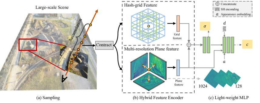
Figure 2: Overview. First, we sample 3D points along the rays emitted from pixels. Second, we parameterize the space into a contracted space for a compact space parameterization. Then, querying the position into the proposed hybrid-representation to extract hash-grid feature and multi-resolution plane features, which are fed into a light-weight MLP to predict the sigma $\sigma$ and the color values $c$ (color MLP requires the additional view directions, appearance embeddings, and plane feature input). Finally, the image colors can be computed by volume rendering.

4 Method

Our goal is to develop an efficient high-resolution feature representation to improve the capacity of fast optimization NeRF methods in representing a large-scale scene.

We start by revisiting the recent efficient hash-grid [31] representation for scene modeling and identify its strengths and limitations. Based on the discussion, we introduce an efficient hybrid representation that enhances the 3D hash-grid feature with high-resolution dense 2D plane features, just with a small increase in the parameters and runtime. Then, we parameterize a large-scale unbounded scene in a contract space [3] to enable a compact space representation. Last, we introduce the network architecture and optimization strategy (see Fig. 2).

4.1 Multi-resolution Hash-grid Representation

Multi-resolution hash-grid [31] is an efficient data structure to represent a scene with high-resolution grids (e.g., $1024$ or even higher resolution) without significantly increasing the parameter number by randomly mapping 3D points to a linear hash table with a fixed size. The parameter number of a multi-resolution hash-grid is bounded by $L\cdot T\cdot F$, where $L$ is the number of the resolution, $T$ and $F$ are the hash table size and feature dimension in each resolution. The suggested configuration is ($L=16,T=2^{19},F=2$) to balance the trade-off between the capacity and efficiency [31], leading to a bound of $2^{24}$ parameters.

Our experiment shows that the hash-grid representation with a highest resolution of $2048$ clearly outperforms the low-resolution dense-grid [45] and TensoRF [7] representation in large-scale scene rendering, demonstrating the resolution of feature resolution plays a very important part in large-scale scene modeling. However, due to the collision problem in random hash mapping, the interpolated feature inevitably contains mixed information for different surface points, limiting the performance of NeRF model. We also observe that increasing the hash table size $T$ can improve the results, but at the cost of a significant increase in parameter number and a longer optimization time [31].

This discussion motivates us to introduce an efficient strategy to boost the hash-grid feature for large-scale scenes just using a small number of parameters and runtime.

4.2 High-resolution 2D Plane Features

Observing that 2D plane features whose parameter grows quadratically with the resolution as $O(N^{2})$ can provide strong information to enable 3D-aware image-synthesis [6] and 3D reconstruction [35], we propose to enhance the hash-grid feature with high-resolution dense plane features for large-scale scene representation.

Orthogonally Placed 2D Plane Features.

We design the plane features as three orthogonally placed planes with a resolution of $N$ and a feature dimension of $F$, then the parameter number for each plane is $N^{2}\cdot F$. For a queried 3D point, we first orthogonally project it on these three planes, and obtain the 2D plane features with bilinear interpolation. We then concatenate the three interpolated features to form a feature vector of length $3\cdot F$.

We are able to scale up the resolution of the dense 2D planes to $1024$. By doing this, our plane representation can provide features in a resolution that “equivalent to” a dense-grid with $2^{30}$ parameters, which is difficult to achieve in a dense-grid due to the significant memory consumption.

Efficient Multi-resolution Design.

However, the feature dimension cannot be too large as the parameters will increase sharply (e.g., setting $F=8$ already results in a parameter number of $8\times 1024\times 1024=2^{23}$), or too small (e.g., $F=2$) as the plane features will not provide useful information (see our ablation study in Table 7). To fulfill the goal of providing high-resolution dense features, we design multi-resolution planes following [31]. Specifically, we adopt a four resolutions configuration $N\in\{128,256,512,1024\}$, each has a feature dimension of $2$, resulting in an $8$ dimension multi-resolution features. This design can effectively boost the hash-grid feature while maintaining a low parameter numbers.

Moreover, as in a large-scale scene, the height of a scene is often smaller than the horizontal length. To reduce the waste of features in the vertical planes, we scale the vertical planes using the camera altitude measurements.

Relation to Previous Work.

Our method is inspired by EG3D [6] which proposes a tri-plane representation, where each plane has a shape of $256\times 256\times 32$, and the interpolated features from three different planes are fused by an add operation for GAN-based image generation. In contrast, our goal is to design efficient high-resolution features for large-scale scene modeling by scaling up the plane feature to $1024$ and using a multi-resolution strategy to maintain a low parameter numbers. Moreover, we use a simple concatenation operation to combine the three interpolated features, as we experimentally find that applying the add operation leads to worse results, which might be explained by the small feature dimension in our representation (i.e., $8$ in ours and $32$ in EG3D).

The recent TensoRF [7] decomposes the radiance fields into several matrices and vectors. However, the matrix has a shape of $N^{2}\cdot R\cdot F$, where $R=192$ is the component number. Compared with the shape of $N^{2}\cdot F$ in our plane feature, the matrices in TensoRF representation cannot be efficiently scaled to a high resolution (e.g., $1024$), making it not suitable for large-scale scene modeling.

4.3 Hybrid of Grid and Plane Features

Given a queried 3D point, we interpolate the hash-grid to get a $32$-dimension grid feature and the orthogonally placed planes to get a $24$-dimension feature. Then these two features are concatenated to form a hybrid feature to be the input of NeRF MLP. Note that there are more sophisticated feature fusion strategies (e.g., MLP fusion) to fuse the hash-grid and plane features. However, to maintain a simple and efficient architecture and also to better demonstrate the effectiveness of our plane features, we just use a simple concatenation.

Compared with the hash-grid that adopts a random mapping hash-function, the orthogonally placed plane representation introduces a structured and high-resolution dense feature, which is complementary to the hash-grid feature, especially in regions with hash collision. As a result, the proposed hybrid feature representation can provide better features for later density and color prediction.

4.4 Scene Space Parameterization

As a large-scale scene covers a wide spatial range and is always unbounded, it is important to parameterize it in a way that it can be represented by a grid-like data structure.

We adopt the mip-NeRF 360 parametrization [3, 46] to represent a unbounded scene. Considering a scene whose center is the origin, we divide the scene into foreground and background regions, separating by a pre-define bound $B$. Given a 3D point, we will first normalize it by $\bm{x}=\bm{x}/B$, and then applied the space contraction:

$$\bm{x}=\begin{cases}\bm{x},&\|\bm{x}\|_{p}\leq 1~{};\\ \left(1+b-\frac{b}{\|\bm{x}\|_{p}}\right)\left(\frac{\bm{x}}{\|\bm{x}\|_{p}}\right),&\|\bm{x}\|_{p}>1~{},\\ \end{cases}$$ (5)

where $p$ denotes $p$-norm, $b$ is to control the size of background space. Following [3], we set $p=2$ and $b=1$.

By doing this, the distribution of points is more compact, where the foreground point (i.e., $\|\bm{x}\|_{p}\leq 1$) is unchanged and a point at infinity will be mapped to the sphere with a radius of $1+b$. This compact representation enable us to represent the scene with the proposed hybrid feature representation (see Fig. 3).

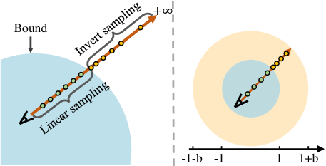
(a) Euclidean space (b) Contracted space

Figure 3: Illustration of the scene parameterization. According to the pre-defined bound, we adopt linear sampling and invert linear sampling for the foreground and background areas, respectively. Then, the sampled points are contracted into a compact space.

4.5 Model Optimization

After defining the hybrid representation and scene parameterization for large-scale scenes, we introduce our network architecture and optimization strategy.

Network Architecture.

Given a 3D point position $\bm{x}_{i}$ and its direction $\bm{d}$ as input, our method first extract the features from the hybrid feature representation. These hybrid features are then fed into a 64-channel two-layer MLP network that regresses the view-independent density value $\sigma_{i}$ and a 15-channel geometry feature.

Then, the view direction encoded with the spherical harmonics function, the per-frame appearance embedding [29], and the plane feature are concatenated with the geometry features to be the input of a 64-channel three-layer network to predict the view-dependent color value. The per-frame appearance embedding is adopted to account for the illumination changes in the captured images. We experimentally found that include the plane feature to the color MLP leads to better results, as discussed in the supplementary material.

Point Sampling.

We adopt a linear sampling strategy for foreground and an invert sampling strategy for the background [46] (see Fig. 3), which satisfies the need of high-quality foreground rendering and covers a wide range of background. In details, we sample $N_{f}=128$ and $N_{b}=64$ points per-ray for these two areas, respectively. We also adopt the coarse-to-fine sampling strategy [30], where the coarse and fine stages have the same number of sampled points, but use the same model to reduce the model size.

Table 2: Quantitative comparison on the testing datasets. * indicates that Mega-NeRF’s results are computed with its released models.

Mill 19 - Building Mill 19 - Rubble UrbanScene3D - Residence UrbanScene3D - Sci-Art UrbanScene3D - Campus Quad 6k Average Method $\uparrow$PSNR $\uparrow$SSIM $\downarrow$LPIPS $\uparrow$PSNR $\uparrow$SSIM $\downarrow$LPIPS $\uparrow$PSNR $\uparrow$SSIM $\downarrow$LPIPS $\uparrow$PSNR $\uparrow$SSIM $\downarrow$LPIPS $\uparrow$PSNR $\uparrow$SSIM $\downarrow$LPIPS $\uparrow$PSNR $\uparrow$SSIM $\downarrow$LPIPS $\downarrow$Time (h) Plenoxels [11] 17.75 0.419 0.670 20.48 0.462 0.658 18.27 0.517 0.579 18.93 0.638 0.528 20.40 0.456 0.780 15.76 0.520 0.665 01:30 TensoRF (VM-192) [7] 18.19 0.416 0.697 20.77 0.452 0.675 18.32 0.498 0.607 18.39 0.594 0.585 17.22 0.418 0.842 14.56 0.512 0.679 01:31 Instant-NGP [31] 18.68 0.439 0.614 21.18 0.497 0.579 18.91 0.554 0.543 19.00 0.644 0.528 16.31 0.527 0.729 14.91 0.509 0.732 01:22 Mega-NeRF* [52] 20.93 0.547 0.504 24.06 0.553 0.516 22.08 0.628 0.489 25.60 0.770 0.390 23.42 0.537 0.618 17.66 0.536 0.616 20:10 Ours 20.99 0.565 0.490 24.08 0.563 0.497 22.41 0.659 0.451 25.56 0.783 0.373 23.46 0.544 0.611 17.67 0.521 0.623 01:35

Independent Background Modeling.

Existing methods show that representing the foreground and background regions independently leads to better results [66, 52]. To increase the model capacity, we utilize two separate models for the foreground and background regions. For the foreground region, we use the proposed hybrid feature representation for feature encoding. For the background region, we only use a hash-grid with a hash table size of $T_{bg}=2^{19}$. Our design can improve the performance without an obvious increase of time costs. Then, points in different regions will be processed by the corresponding models.

Loss Function.

Given multiple 3D points sampled from a view ray $\bm{r}$, volume rendering will be utilized to produce the pixel color. We adopt the mean square error (MSE) between the rendered color $\hat{C}(\bm{r})$ and the ground-truth color $C(\bm{r})$ as the loss function:

$$Loss=\sum_{\bm{r}\in\mathcal{R}}{\|\hat{C}(\bm{r})-C(\bm{r})\|}_{2}^{2},$$ (6)

where $\mathcal{R}$ is the sampled ray set.

5 Experiments

Datasets.

Following Mega-NeRF [52], we evaluate our GP-NeRF on three public large-scale datasets, namely the Mill19 [52], Quad6k [9], and UrbanScene3D [25] datasets, with the camera poses refined by PixSFM [26]. Mill19 dataset is proposed by Mega-NeRF [52], which includes Mill19-Building and Mill19-Rubble, covering about $250\times 400\ m^{2}$ large areas. Quad6k dataset is a large-scale Structure-from-Motion (SfM) dataset containing about 5100 images of Cornell University Arts Quad. Following [52], we adopt three urban scenes from UrbanScene3D dataset, which provide high-resolution images from drones.

Implementation Details.

We implemented our method with PyTorch [34] and used the Adam optimizer [21] with default parameters. Our model was trained with $100$K iteration using a batch size of $5\times 1024$ rays. The learning rate was set to 0.001. Following the practice in [31], the hyper-parameter of hash table size is set to $L=16,T=2^{19},F=2$. The lowest and highest resolutions are set to $16$ and $2048$, respectively. The runtime was measured on an NVIDIA GeForce RTX 3090 GPU.

Evaluation Metrics.

We evaluate the existing methods and our method in terms of PSNR, SSIM [55], and the VGG implementation of LPIPS [67].

Table 3: Comparison between our hybrid-representation and existing feature representations. We compare with three baselines that replace the hybrid-representation in our method with the dense-grid [45, 11], the pure hash-grid [31], and the TensoRF (VM-192) [7].

Mill 19 - Building Mill 19 - Rubble UrbanScene3D - Residence UrbanScene3D - Sci-Art UrbanScene3D - Campus Quad 6k Timing Method $\uparrow$PSNR $\uparrow$SSIM $\downarrow$LPIPS $\uparrow$PSNR $\uparrow$SSIM $\downarrow$LPIPS $\uparrow$PSNR $\uparrow$SSIM $\downarrow$LPIPS $\uparrow$PSNR $\uparrow$SSIM $\downarrow$LPIPS $\uparrow$PSNR $\uparrow$SSIM $\downarrow$LPIPS $\uparrow$PSNR $\uparrow$SSIM $\downarrow$LPIPS $\downarrow$Time (h) Ours w/ TensoRF [7] 19.44 0.457 0.615 22.82 0.485 0.621 21.17 0.573 0.552 22.59 0.656 0.535 22.05 0.487 0.720 15.15 0.517 0.666 03:34 Ours w/ dense-grid [45, 11] 18.95 0.437 0.636 22.46 0.464 0.649 20.43 0.541 0.571 21.24 0.629 0.560 21.61 0.475 0.730 14.61 0.508 0.687 01:31 Ours w/ hash-grid [31] 20.58 0.539 0.514 23.77 0.546 0.516 22.05 0.634 0.478 25.06 0.770 0.391 22.96 0.528 0.638 17.31 0.516 0.636 01:21 Ours w/ hash-grid (01:30) 20.66 0.545 0.509 23.77 0.548 0.515 22.06 0.636 0.477 25.15 0.772 0.388 23.07 0.530 0.633 17.34 0.516 0.631 01:34 Ours 20.99 0.565 0.490 24.08 0.563 0.497 22.41 0.659 0.451 25.56 0.783 0.373 23.46 0.544 0.611 17.67 0.521 0.623 01:35

(a) Ours w/ dense-grid (b) Ours w/ TensoRF (c) Ours w/ hash-grid (d) GP-NeRF (ours) (e) Mega-NeRF (f) Ground Truth

Figure 4: Qualitative results on the Mill19-Rubble and UrbanScene3D-Campus dataset.

5.1 Evaluation

Comparison with Existing Methods.

We first compare our method with existing methods to verify its effectiveness. Specifically, we compare with the state-of-the-art Mega-NeRF [52] and fast NeRF methods (Plenoxels [11], TensoRF [7], and Instant-NGP [31]). The training time are measured by training on the same amount of data.

We can see from Table 2 that our method achieves the best results on five of the six scenes. Compared with Mega-NeRF which requires about one day’s training with 8 GPUs, our method achieves a fast convergence speed of 1.5 hours using a single GPU, while maintaining comparable or even better results. The reason is that our method only use a single 5-layer network with 64 channels and an efficient hybrid feature representation for feature interpolation, while Mega-NeRF uses large 9-layer MLPs with 256 channels for predictions.

Despite enjoying fast training convergence, existing fast NeRF methods [11, 7, 31] achieve poor rendering quality. It is because these methods are not designed for large-scale unbounded scenes with illumination changes and suffer from low-resolution representation.

Comparison with Other Feature Representations.

To further demonstrate the effectiveness of our hybrid feature representation, we design three baseline methods. Specifically, we replace the proposed hybrid feature representation of our method with the dense-grid (resolution is $160^{3}$) [45, 11] and pure hash-grid [31] representation. In addition, we adopt the VM-192 variant of TensoRF with a resolution of $300^{3}$ voxels [7]. To have a fair comparison, other parts of the methods are kept the same. We also apply the feature space scaling according to the camera altitude measurement for the baseline methods for fair comparisons. Quantitative results in Table 3 show that the results of methods with dense-grid and TensoRF representation are worse, indicating that they are not suitable for large-scale scenes as their feature resolutions are low. Compared with these two methods, our method achieves much more accurate rendering results, with comparable or smaller parameters (i.e., ours is 33.0M, Ours w/ TensoRF is 34.8M, and Ours w/ dense-grid is 98.4M).

Our method also consistently outperforms Ours w/ hash-grid on all six datasets. We notice that the hash-grid method finishes training with less time, we therefore design experiments to train the hash-grid method with the same time as ours for a fair comparison, namely Ours w/ hash-grid (01:30) in Table 3. The results show that the performance of hash-grid method improves with a longer training time, but its results are still far behind our method, further demonstrating the effectiveness of our method.

Figure 4 shows the qualitative comparison. We can see that the baselines based on low-resolution features, e.g. Ours w/ TensoRF and dense-grid, produce blurry results, while Ours w/ hash-grid produces better results with high-resolution hash-grid. However, at the presence of collision, the rendering details are still blurry. In contrast, we design the multi-scale high-resolution dense plane and utilize the hybrid-representation to enhance the hash-grid feature, leading to better results (e.g. the railway track in the Mill19-Rubble dataset).

5.2 Ablation study

In this section, we conduct ablation studies to evaluate the proposed GP-NeRF on two representative scenes, Mill19-Rubble [52] and UrbanScene3D-Residence [25].

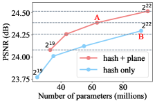
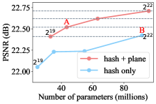
(a) Rubble (b) Residence

Figure 5: Quantitative results of integrating the plane feature with hash-grids that have a hash table size $T$ ranged from $2^{19}$ to $2^{22}$.

Effectiveness of the Plane Feature.

To verify the effectiveness of the proposed hybrid feature representation, we integrate our plane features with hash-grid with different hash table sizes (i.e., from $2^{19}$ to $2^{22}$) and compare them with methods using only hash-grid features, and the results are summarized in Fig. 5. We can see that as the hash table size improves, the results of hash-grid only method increase but with a significant increase in model size. It can be clearly seen that the performance of models with a hybrid of hash-grid feature (with different hash table sizes) and plane features exceed the corresponding pure hash-grid results. Notably, the hybrid representation can achieve better results using much fewer number of parameters than a pure hash-grid with higher table size (e.g., comparing the point $A$ and $B$ in Fig. 5).

To better verify the effectiveness of our plane feature, we remove the hash-grid and only use plane features for feature encoding. Experiment with ID 0 in Table 4 shows that the pure plane features can also achieve respectable results (see Fig. 6 for visual results). Furthermore, we replace the plane feature in our hybrid representation with the dense-grid ($90^{3}$) and TensoRF (VM-192, $210^{3}$) that has comparable parameters as our method (i.e., 33.0M). Experiments with IDs 1-4 in Table 4 shows that integrating hash-grid with the low-resolution dense-grid or TensoRF cannot consistently improve the results and might lead to worse results (see the average PSNR), indicating that the high-resolution plane features help to resolve the collision problem and the improvement comes from our design rather than an increase of parameters. Both the quantitative and qualitative results reiterate that the plane features provide strong information for the scene geometry and appearance and is complementary to the hash-grid features.

Table 4: Effectiveness of the model design.

			Rubble		Residence		Average
ID	Model	# Param	PSNR	SSIM	PSNR	SSIM	PSNR	SSIM
0	Plane only	16.8M	22.75	0.493	20.61	0.554	21.68	0.524
1	Hash-grid ($2^{19}$)	24.6M	23.77	0.546	22.05	0.634	22.91	0.590
2	Hash-grid + Dense	33.3M	23.82	0.554	21.86	0.639	22.84$\downarrow$	0.597
3	Hash-grid + TensoRF	33.1M	23.77	0.547	22.02	0.634	22.90$\downarrow$	0.591
4	Hash-grid + Plane (Ours)	33.0M	24.08	0.565	22.41	0.659	23.25$\uparrow$	0.612

(a) Plane only (b) Hash-grid (c) Hash-grid + Plane (d) GT

Figure 6: Effectiveness of the plane feature.

Effects of Plane Feature Dimension.

In Table 7, we first conduct experiments with IDs 0-1 to investigate the influence of feature dimension in a single-resolution plane representation. We can see that the result of a single-resolution plane with small feature dimension (e.g., $2$) is worse, and using a high feature dimension (e.g., $8$) can achieve good PSNR results, but the increase in the number of parameters is also significant. Experiments with ID 2-3 in Table 7 show that multi-resolution planes with small resolution can also achieve good results while maintaining a small parameter number. These results justify the design of our multi-resolution plane features, which strikes a good balance between the performance and parameters.

Effects of Plane Feature Resolution.

To investigate the influence of the resolution of plane features, we compare results of plane features with different highest resolutions (the base resolution is $128$). Table 7 shows that there is a tendency that the larger the highest resolution is, the better performance achieves, which is a trade-off between the increase of parameters and performance. This also demonstrates the effectiveness of plane features.

Table 5: Effects of the feature dimension per resolution and the multi-resolution design in the plane feature representation.

				Rubble		Residence
IDs	Resolutions / Dim.	Total Dim.	# Param	PSNR	SSIM	PSNR	SSIM
0	{1024} / 2	2	30.9M	23.92	0.556	22.32	0.652
1	{1024} / 8	8	49.8M	24.14	0.570	22.60	0.670
2	{128,1024} / 4	8	37.4M	24.10	0.566	22.41	0.661
3	{128,256,512,1024} / 2	8	33.0M	24.08	0.565	22.41	0.659

Table 6: Effects of the highest resolution in plane features.

		Rubble		Residence
Model	# Param	PSNR	SSIM	PSNR	SSIM
Hash-grid $2^{19}$ + plane 256	25.5M	23.97	0.557	22.20	0.643
Hash-grid $2^{19}$ + plane 512	27.1M	24.04	0.559	22.16	0.648
Hash-grid $2^{19}$ + plane 1024	33.0M	24.08	0.565	22.41	0.659
Hash-grid $2^{19}$ + plane 2048	54.5M	24.32	0.589	22.43	0.673

Table 7: Results of Mega-NeRF variants trained with 8 GPUs.

	Building		Rubble		Residence		Campus
Model	PSNR	SSIM	PSNR	SSIM	PSNR	SSIM	PSNR	SSIM
Mega-NeRF (1 day)	20.93	0.547	24.06	0.553	22.08	0.628	23.42	0.537
Mega-NeRF (1.5 h)	19.10	0.436	22.29	0.462	20.08	0.516	21.67	0.476
Mega-NeRF w/ INGP (1.5 h)	21.30	0.601	24.47	0.607	22.36	0.671	23.59	0.565
Mega-NeRF w/ GP-NeRF (1.5 h)	21.71	0.619	24.80	0.623	22.81	0.698	23.94	0.580

5.3 GP-NeRF as the Local Radiance Field

As a general NeRF variant, our GP-NeRF can also be adopted as the local radiance field in Mega-NeRF’s partition training framework [52] to further improve the performance. We trained two Mega-NeRF variants with GP-NeRF and Instance-NGP [31] (for purpose of comparison) as the local NeRF. Table 7 shows that adopting our GP-NeRF as the local radiance field achieves the best results in $1.5$ hours, clearly outperforms Mega-NeRF and the Instant-NGP variant, verifying the design of our method.

6 Conclusion

In this paper, we have presented a hybrid feature representation for the neural radiance fields to enable efficient large-scale scene modeling. Our hybrid representation enhances the hash-grid feature with orthogonally placed high-resolution and dense plane features, especially for surface regions with hash collisions. Compared with directly scaling up the hash table size in the hash-grid, our representation can achieve higher accuracy with comparable runtime while using much fewer parameters. Based on our hybrid representation, we propose a new variant of NeRF, called GP-NeRF, to represent large-scale unbounded scenes. Compared with the existing method [52] that requires one day’s training on 8 GPUs, our method achieves comparable or even better results with $1.5$ hours on a single GPU, which is especially useful for scenarios with limited computing resources.

Limitations.

Despite the significant acceleration of optimization achieved for large-scale scene representation, our method still cannot achieve real-time scene reconstruction. Moreover, our method does not explicitly model dynamic objects and thus cannot represent a dynamic scene. We would like to address these two problems in the future.

References

- [1] Sameer Agarwal, Yasutaka Furukawa, Noah Snavely, Ian Simon, Brian Curless, Steven M Seitz, and Richard Szeliski. Building rome in a day. Communications of the ACM, 2011.
- [2] Jonathan T Barron, Ben Mildenhall, Matthew Tancik, Peter Hedman, Ricardo Martin-Brualla, and Pratul P Srinivasan. Mip-NeRF: A multiscale representation for anti-aliasing neural radiance fields. In ICCV, 2021.
- [3] Jonathan T Barron, Ben Mildenhall, Dor Verbin, Pratul P Srinivasan, and Peter Hedman. Mip-nerf 360: Unbounded anti-aliased neural radiance fields. In CVPR, 2022.
- [4] Mark Boss, Raphael Braun, Varun Jampani, Jonathan T Barron, Ce Liu, and Hendrik Lensch. NeRD: Neural reflectance decomposition from image collections. In ICCV, 2021.
- [5] Ang Cao and Justin Johnson. Hexplane: a fast representation for dynamic scenes. arXiv preprint arXiv:2301.09632, 2023.
- [6] Eric R Chan, Connor Z Lin, Matthew A Chan, Koki Nagano, Boxiao Pan, Shalini De Mello, Orazio Gallo, Leonidas J Guibas, Jonathan Tremblay, Sameh Khamis, et al. Efficient geometry-aware 3d generative adversarial networks. In CVPR, 2022.
- [7] Anpei Chen, Zexiang Xu, Andreas Geiger, Jingyi Yu, and Hao Su. Tensorf: Tensorial radiance fields. arXiv preprint arXiv:2203.09517, 2022.
- [8] Anpei Chen, Zexiang Xu, Fuqiang Zhao, Xiaoshuai Zhang, Fanbo Xiang, Jingyi Yu, and Hao Su. MVSNerf: Fast generalizable radiance field reconstruction from multi-view stereo. In ICCV, 2021.
- [9] David Crandall, Andrew Owens, Noah Snavely, and Dan Huttenlocher. Discrete-continuous optimization for large-scale structure from motion. In CVPR, 2011.
- [10] Sara Fridovich-Keil, Giacomo Meanti, Frederik Warburg, Benjamin Recht, and Angjoo Kanazawa. K-planes: Explicit radiance fields in space, time, and appearance. arXiv preprint arXiv:2301.10241, 2023.
- [11] Sara Fridovich-Keil, Alex Yu, Matthew Tancik, Qinhong Chen, Benjamin Recht, and Angjoo Kanazawa. Plenoxels: Radiance fields without neural networks. In CVPR, 2022.
- [12] Christian Früh and Avideh Zakhor. An automated method for large-scale, ground-based city model acquisition. IJCV, 2004.
- [13] Yasutaka Furukawa, Brian Curless, Steven M Seitz, and Richard Szeliski. Towards internet-scale multi-view stereo. 2010.
- [14] Yasutaka Furukawa and Jean Ponce. Accurate, dense, and robust multi-view stereopsis. TPAMI, 2010.
- [15] Xuan Gao, Chenglai Zhong, Jun Xiang, Yang Hong, Yudong Guo, and Juyong Zhang. Reconstructing personalized semantic facial nerf models from monocular video. TOG, 2022.
- [16] Stephan J Garbin, Marek Kowalski, Matthew Johnson, Jamie Shotton, and Julien Valentin. Fastnerf: High-fidelity neural rendering at 200fps. In ICCV, 2021.
- [17] Xiang Guo, Guanying Chen, Yuchao Dai, Xiaoqing Ye, Jiadai Sun, Xiao Tan, and Errui Ding. Neural deformable voxel grid for fast optimization of dynamic view synthesis. In ACCV, 2022.
- [18] Peter Hedman, Pratul P Srinivasan, Ben Mildenhall, Jonathan T Barron, and Paul Debevec. Baking neural radiance fields for real-time view synthesis. In ICCV, 2021.
- [19] Tao Hu, Shu Liu, Yilun Chen, Tiancheng Shen, and Jiaya Jia. Efficientnerf efficient neural radiance fields. In CVPR, 2022.
- [20] James T Kajiya and Brian P Von Herzen. Ray tracing volume densities. ACM SIGGRAPH computer graphics, 1984.
- [21] Diederik P Kingma and Jimmy Ba. Adam: A method for stochastic optimization. In ICLR, 2015.
- [22] Xiaowei Li, Changchang Wu, Christopher Zach, Svetlana Lazebnik, and Jan-Michael Frahm. Modeling and recognition of landmark image collections using iconic scene graphs. In ECCV, 2008.
- [23] Zhengqi Li, Simon Niklaus, Noah Snavely, and Oliver Wang. Neural scene flow fields for space-time view synthesis of dynamic scenes. In CVPR, 2021.
- [24] Haotong Lin, Sida Peng, Zhen Xu, Yunzhi Yan, Qing Shuai, Hujun Bao, and Xiaowei Zhou. Efficient neural radiance fields for interactive free-viewpoint video. In SIGGRAPH Aisa Conference, 2022.
- [25] Liqiang Lin, Yilin Liu, Yue Hu, Xingguang Yan, Ke Xie, and Hui Huang. Capturing, reconstructing, and simulating: the urbanscene3d dataset. In ECCV, 2022.
- [26] Philipp Lindenberger, Paul-Edouard Sarlin, Viktor Larsson, and Marc Pollefeys. Pixel-perfect structure-from-motion with featuremetric refinement. In ICCV, 2021.
- [27] Lingjie Liu, Jiatao Gu, Kyaw Zaw Lin, Tat-Seng Chua, and Christian Theobalt. Neural sparse voxel fields. In NIPS, 2020.
- [28] Stephen Lombardi, Tomas Simon, Gabriel Schwartz, Michael Zollhoefer, Yaser Sheikh, and Jason Saragih. Mixture of volumetric primitives for efficient neural rendering. TOG, 2021.
- [29] Ricardo Martin-Brualla, Noha Radwan, Mehdi SM Sajjadi, Jonathan T Barron, Alexey Dosovitskiy, and Daniel Duckworth. NeRF in the wild: Neural radiance fields for unconstrained photo collections. In CVPR, 2021.
- [30] Ben Mildenhall, Pratul P Srinivasan, Matthew Tancik, Jonathan T Barron, Ravi Ramamoorthi, and Ren Ng. NeRF: Representing scenes as neural radiance fields for view synthesis. In ECCV, 2020.
- [31] Thomas Müller, Alex Evans, Christoph Schied, and Alexander Keller. Instant neural graphics primitives with a multiresolution hash encoding. arXiv preprint arXiv:2201.05989, 2022.
- [32] Thomas Neff, Pascal Stadlbauer, Mathias Parger, Andreas Kurz, Joerg H Mueller, Chakravarty R Alla Chaitanya, Anton Kaplanyan, and Markus Steinberger. Donerf: Towards real-time rendering of compact neural radiance fields using depth oracle networks. CGF, 2021.
- [33] Michael Niemeyer, Lars Mescheder, Michael Oechsle, and Andreas Geiger. Differentiable volumetric rendering: Learning implicit 3d representations without 3d supervision. In CVPR, 2020.
- [34] Adam Paszke, Sam Gross, Soumith Chintala, and Gregory Chanan. PyTorch: Tensors and dynamic neural networks in Python with strong GPU acceleration, 2017.
- [35] Songyou Peng, Michael Niemeyer, Lars Mescheder, Marc Pollefeys, and Andreas Geiger. Convolutional occupancy networks. In ECCV, 2020.
- [36] Albert Pumarola, Enric Corona, Gerard Pons-Moll, and Francesc Moreno-Noguer. D-NeRF: Neural radiance fields for dynamic scenes. In CVPR, 2021.
- [37] Christian Reiser, Songyou Peng, Yiyi Liao, and Andreas Geiger. Kilonerf: Speeding up neural radiance fields with thousands of tiny mlps. In ICCV, 2021.
- [38] Konstantinos Rematas, Andrew Liu, Pratul P Srinivasan, Jonathan T Barron, Andrea Tagliasacchi, Thomas Funkhouser, and Vittorio Ferrari. Urban radiance fields. In CVPR, 2022.
- [39] Gernot Riegler and Vladlen Koltun. Stable view synthesis. In CVPR, 2021.
- [40] Johannes L Schonberger and Jan-Michael Frahm. Structure-from-motion revisited. In CVPR, 2016.
- [41] Ruizhi Shao, Zerong Zheng, Hanzhang Tu, Boning Liu, Hongwen Zhang, and Yebin Liu. Tensor4d: Efficient neural 4d decomposition for high-fidelity dynamic reconstruction and rendering. arXiv preprint arXiv:2211.11610, 2022.
- [42] Harry Shum and Sing Bing Kang. Review of image-based rendering techniques. In VCIP, 2000.
- [43] Vincent Sitzmann, Julien Martel, Alexander Bergman, David Lindell, and Gordon Wetzstein. Implicit neural representations with periodic activation functions. In NIPS, 2020.
- [44] Noah Snavely, Steven M. Seitz, and Richard Szeliski. Photo tourism: Exploring photo collections in 3d. In SIGGRAPH, 2006.
- [45] Cheng Sun, Min Sun, and Hwann-Tzong Chen. Direct voxel grid optimization: Super-fast convergence for radiance fields reconstruction. In CVPR, 2022.
- [46] Cheng Sun, Min Sun, and Hwann-Tzong Chen. Improved direct voxel grid optimization for radiance fields reconstruction. arXiv preprint arXiv:2206.05085, 2022.
- [47] Matthew Tancik, Vincent Casser, Xinchen Yan, Sabeek Pradhan, Ben Mildenhall, Pratul P Srinivasan, Jonathan T Barron, and Henrik Kretzschmar. Block-nerf: Scalable large scene neural view synthesis. In CVPR, 2022.
- [48] Ayush Tewari, Ohad Fried, Justus Thies, Vincent Sitzmann, Stephen Lombardi, Kalyan Sunkavalli, Ricardo Martin-Brualla, Tomas Simon, Jason Saragih, Matthias Nießner, et al. State of the art on neural rendering. CGF, 2020.
- [49] Ayush Tewari, O Fried, J Thies, V Sitzmann, S Lombardi, Z Xu, T Simon, M Nießner, E Tretschk, L Liu, et al. Advances in neural rendering. In SIGGRAPH, 2021.
- [50] Edgar Tretschk, Ayush Tewari, Vladislav Golyanik, Michael Zollhöfer, Christoph Lassner, and Christian Theobalt. Non-rigid neural radiance fields: Reconstruction and novel view synthesis of a dynamic scene from monocular video. In ICCV, 2021.
- [51] Alex Trevithick and Bo Yang. GRF: Learning a general radiance field for 3d representation and rendering. In ICCV, 2021.
- [52] Haithem Turki, Deva Ramanan, and Mahadev Satyanarayanan. Mega-nerf: Scalable construction of large-scale nerfs for virtual fly-throughs. In CVPR, 2022.
- [53] Liao Wang, Jiakai Zhang, Xinhang Liu, Fuqiang Zhao, Yanshun Zhang, Yingliang Zhang, Minye Wu, Jingyi Yu, and Lan Xu. Fourier plenoctrees for dynamic radiance field rendering in real-time. In CVPR, 2022.
- [54] Qianqian Wang, Zhicheng Wang, Kyle Genova, Pratul P Srinivasan, Howard Zhou, Jonathan T Barron, Ricardo Martin-Brualla, Noah Snavely, and Thomas Funkhouser. IBRNet: Learning multi-view image-based rendering. In CVPR, 2021.
- [55] Zhou Wang, Alan C Bovik, Hamid R Sheikh, and Eero P Simoncelli. Image quality assessment: from error visibility to structural similarity. TIP, 2004.
- [56] Suttisak Wizadwongsa, Pakkapon Phongthawee, Jiraphon Yenphraphai, and Supasorn Suwajanakorn. Nex: Real-time view synthesis with neural basis expansion. In CVPR, 2021.
- [57] Liwen Wu, Jae Yong Lee, Anand Bhattad, Yu-Xiong Wang, and David Forsyth. Diver: Real-time and accurate neural radiance fields with deterministic integration for volume rendering. In CVPR, 2022.
- [58] Xiuchao Wu, Jiamin Xu, Zihan Zhu, Hujun Bao, Qixing Huang, James Tompkin, and Weiwei Xu. Scalable neural indoor scene rendering. TOG, 2022.
- [59] Yuanbo Xiangli, Linning Xu, Xingang Pan, Nanxuan Zhao, Anyi Rao, Christian Theobalt, Bo Dai, and Dahua Lin. Bungeenerf: Progressive neural radiance field for extreme multi-scale scene rendering. In ECCV, 2022.
- [60] Yiheng Xie, Towaki Takikawa, Shunsuke Saito, Or Litany, Shiqin Yan, Numair Khan, Federico Tombari, James Tompkin, Vincent Sitzmann, and Srinath Sridhar. Neural fields in visual computing and beyond. CGF, 2022.
- [61] Qiangeng Xu, Zexiang Xu, Julien Philip, Sai Bi, Zhixin Shu, Kalyan Sunkavalli, and Ulrich Neumann. Point-nerf: Point-based neural radiance fields. In CVPR, 2022.
- [62] Wenqi Yang, Guanying Chen, Chaofeng Chen, Zhenfang Chen, and Kwan-Yee K Wong. PS-NeRF: Neural inverse rendering for multi-view photometric stereo. In ECCV, 2022.
- [63] Lior Yariv, Yoni Kasten, Dror Moran, Meirav Galun, Matan Atzmon, Ronen Basri, and Yaron Lipman. Multiview neural surface reconstruction by disentangling geometry and appearance. In NIPS, 2020.
- [64] Alex Yu, Ruilong Li, Matthew Tancik, Hao Li, Ren Ng, and Angjoo Kanazawa. Plenoctrees for real-time rendering of neural radiance fields. In ICCV, 2021.
- [65] Alex Yu, Vickie Ye, Matthew Tancik, and Angjoo Kanazawa. pixelnerf: Neural radiance fields from one or few images. In CVPR, 2021.
- [66] Kai Zhang, Gernot Riegler, Noah Snavely, and Vladlen Koltun. NeRF++: Analyzing and improving neural radiance fields. arXiv preprint arXiv:2010.07492, 2020.
- [67] Richard Zhang, Phillip Isola, Alexei A Efros, Eli Shechtman, and Oliver Wang. The unreasonable effectiveness of deep features as a perceptual metric. In CVPR, 2018.
- [68] Xiaoshuai Zhang, Sai Bi, Kalyan Sunkavalli, Hao Su, and Zexiang Xu. Nerfusion: Fusing radiance fields for large-scale scene reconstruction. In CVPR, 2022.
- [69] Xiuming Zhang, Pratul P Srinivasan, Boyang Deng, Paul Debevec, William T Freeman, and Jonathan T Barron. NeRFactor: Neural factorization of shape and reflectance under an unknown illumination. TOG, 2021.
- [70] Siyu Zhu, Runze Zhang, Lei Zhou, Tianwei Shen, Tian Fang, Ping Tan, and Long Quan. Very large-scale global sfm by distributed motion averaging. In CVPR, 2018.