The Complexity of Geodesic Spanners

Abstract

A geometric $t$-spanner for a set $S$ of $n$ point sites is an edge-weighted graph for which the (weighted) distance between any two sites $p,q\in S$ is at most $t$ times the original distance between $p$ and $q$. We study geometric $t$-spanners for point sets in a constrained two-dimensional environment $P$. In such cases, the edges of the spanner may have non-constant complexity. Hence, we introduce a novel spanner property: the spanner complexity, that is, the total complexity of all edges in the spanner. Let $S$ be a set of $n$ point sites in a simple polygon $P$ with $m$ vertices. We present an algorithm to construct, for any constant $\varepsilon>0$ and fixed integer $k\geq 1$, a $(2k+\varepsilon)$-spanner with complexity $O(mn^{1/k}+n\log^{2}n)$ in $O(n\log^{2}n+m\log n+K)$ time, where $K$ denotes the output complexity. When we consider sites in a polygonal domain $P$ with holes, we can construct such a $(2k+\varepsilon)$-spanner of similar complexity in $O(n^{2}\log m+nm\log m+K)$ time. Additionally, for any constant $\varepsilon\in(0,1)$ and integer constant $t\geq 2$, we show a lower bound for the complexity of any $(t-\varepsilon)$-spanner of $\Omega(mn^{1/(t-1)}+n)$.

1 Introduction

In the design of networks on a set of nodes, we often consider two criteria: few connections between the nodes, and small distances. Spanners are geometric networks on point sites that replace the small distance criterion by a small detour criterion. Formally, a geometric $t$-spanner for a set $S$ of $n$ point sites is an edge-weighted graph $\mathcal{G}=(S,E)$ for which the (weighted) distance $d_{\mathcal{G}}(p,q)$ between any two sites $p,q\in S$ is at most $t\cdot d(p,q)$, where $d(p,q)$ denotes the distance between $p$ and $q$ in the distance metric we consider [32]. The smallest value $t$ for which a graph $\mathcal{G}$ is a $t$-spanner is called the spanning ratio of $\mathcal{G}$. The number of edges in the spanner is called the size of the spanner.

In the real world, spanners are often constructed in some sort of environment. For example, we might want to connect cities by a railway network, where the tracks should avoid obstacles such as mountains or lakes. One way to model such an environment is by a polygonal domain. In this paper, we study the case where the sites lie in a polygonal domain $P$ with $m$ vertices and $h$ holes, and we measure the distance between two points $p,q$ by their geodesic distance: the length of the shortest path between $p$ and $q$ fully contained within $P$. An example of such a spanner is provided in Figure 1.

Figure 1: A spanner on a set of point sites in a polygonal domain. Because of the orange edges, the spanner has a relatively high complexity.

The spanning ratio and the size of spanners are not the only properties of interest. Many different properties have been studied, such as total weight (or lightness), maximum degree, (hop) diameter, and fault-tolerance [4, 9, 11, 14, 20, 29, 30, 35]. When we consider distance metrics for which the edges in the spanner no longer have constant complexity, another interesting property of spanners arises: the spanner complexity, i.e. the total complexity of all edges in the spanner. In our railway example, this corresponds to the total number of bends in the tracks. A spanner with a low number of bends may be desired, as trains can drive faster on straight tracks, and it makes construction cheaper. In this paper, we study this novel property for point sites in a polygonal domain, where the complexity of an edge is simply the number of line segments in the path. In this setting, a single edge may have complexity $\Theta(m)$. Naively, a spanner of size $E$ could thus have complexity $\Theta(mE)$. Our goal is to compute an $O(1)$-spanner of size $O(n\operatorname{polylog}n)$ with small complexity, preferably near linear in both $n$ and $m$.

When studying spanning trees of points, two variants exist: with or without Steiner points. The same is true for spanners, where Steiner points can be used to obtain lighter and sparser spanners [6, 29]. In this paper we focus on the variant where Steiner points are not allowed, leaving the other variant to future research.

Related work.

For the Euclidean distance in $\mathbb{R}^{d}$, and any fixed $\varepsilon>0$, there is a $(1+\varepsilon)$-spanner of size $O(n/\varepsilon^{d-1})$ [35]. For the more general case of metric spaces of bounded doubling dimension we can also construct a $(1+\varepsilon)$-spanner of size $O(n/\varepsilon^{O(d)})$ [13, 22, 25]. These results do not apply when the sites lie in a polygon, and we measure their distances using the geodesic distance. Abam et al. [1] show there is a set of $n$ sites in a simple polygon $P$ for which any geodesic $(2-\varepsilon)$-spanner has $\Omega(n^{2})$ edges. They also construct a geodesic $(\sqrt{10}+\varepsilon)$-spanner of size $O(n\log^{2}n)$ for sites in a simple polygon, and a geodesic $(5+\varepsilon)$-spanner of size $O(n\sqrt{h}\log^{2}n)$ for sites in a polygonal domain. Recently, Abam et al. [3] showed that a geodesic $(2+\varepsilon)$-spanner with $O(n\log n)$ edges exists for points on a polyhedral terrain, thereby almost closing the gap between the upper and lower bound on the spanning ratio. However, they show only the existence of such a spanner, and leave constructing one open. Moreover, all of these spanners can have high, $\Omega(nm)$, complexity.

Abam et al. [3] make use of spanners on an additively weighted point set in $\mathbb{R}^{d}$. In this setting, the distance between two sites $p,q$ is $w(p)+|pq|+w(q)$ for $p\neq q$, where $w(p)$ is the non-negative weight of a site $p\in S$ and $|pq|$ denotes the Euclidean distance, and $0$ for $p=q$. Such additively weighted spanners were studied before by Abam et al. [2], who obtain an $O(5+\varepsilon)$-spanner of linear size, and an $O(2+\varepsilon)$-spanner of size $O(n\log n)$. They also provide a lower bound of $\Omega(n^{2})$ on the size of any $(2-\varepsilon)$-spanner. Abam et al. [3] improve these results and obtain a nearly optimal additively weighted $(2+\varepsilon)$-spanner of size $O(n)$.

The other key ingredient for the geodesic $(2+\varepsilon)$-spanner of Abam et al. [3] is a balanced shortest-path separator. Such a separator consists of either a single shortest path between two points on the boundary of the terrain, or three shortest paths that form a shortest-path triangle. This separator partitions the terrain into two subterrains, and we call it balanced when each of these terrains contains roughly half of the sites in $S$. In their constructive proof for the existence of such a balanced separator, they assume that the three shortest paths in a shortest-path triangle are disjoint, except for their mutual endpoints. However, during their construction it can actually happen that these paths are not disjoint. When this happens, it is unclear exactly how to proceed. Just like for the $(2+\varepsilon)$-spanner, the computation of a balanced separator is left for future research. We show how to get rid of the assumption that the shortest paths are disjoint, and thereby confirm the result claimed by Abam et al. [3].

Next to spanners on the complete Euclidean geometric graph, spanners under line segment constraints were studied [8, 10, 12, 16, 17]. In this setting, a set $C$ of line segment constraints is provided, where each line segment is between two sites in $S$ and no two line segments properly intersect. The goal is to construct a spanner on the visibility graph of $S$ with respect to $C$. Clarkson [16] showed how to construct a linear sized $(1+\varepsilon)$-spanner for this graph. Later, (constrained) Yao- and $\Theta$-graphs were also considered in this setting [8, 12]. If the segments in $C$ form a polygonal domain $P$, this setting is similar to ours, except that all vertices of $P$ are included as sites in $S$. Thus the complexity of each edge is constant, and additionally it is required that there are short paths between the vertices of $P$.

Low complexity paths are studied in the minimum-link path problem. In this problem, the goal is to find a path the uses a minimal number of links (edges) between two sites in a domain, for example a simple polygon [34, 36, 21, 26]. Generally, this problem focuses only on the complexity of the path, with no restriction on the length of the path. Mitchell et al. [33] consider the related problem of finding the shortest path with at most $k$ edges between two points $p,q$ in a simple polygon. They give an algorithm to compute a $k$-link path with length at most $(1+\varepsilon)$ times the length of the shortest $k$-link path, for any $\varepsilon>0$. This result can not be applied to our setting, as the length of our paths should be bounded in terms of $d(p,q)$, i.e. the shortest $m$-link path, instead of the shortest $k$-link path.

Our results.

We first consider the simple setting where the sites lie in a simple polygon, i.e. a polygonal domain without holes. We show that in this setting any $(3-\varepsilon)$-spanner may have complexity $\Omega(nm)$, thus implying that the $(2+\varepsilon)$-spanner of Abam et al. [3] may also have complexity $\Omega(nm)$, despite having $O(n\log n)$ edges.

To improve this complexity, we first introduce a simple 2-spanner with $O(n\log n)$ edges for an additively weighted point set in a 1-dimensional Euclidean space; see Section 2. In Section 3, we use this result to obtain a geodesic $2\sqrt{2}$-spanner with $O(n\log^{2}n)$ edges for a point set in a simple polygon. We recursively split the polygon by a chord $\lambda$ such that each subpolygon contains roughly half of the sites, and build a 1-dimensional spanner on the sites projected to $\lambda$. We then extend this spanner into one that also has bounded complexity. For any constant $\varepsilon>0$ and fixed integer $k\geq 1$, we obtain a $(2k+\varepsilon)$-spanner with complexity $O(mn^{1/k}+n\log^{2}n)$. Furthermore, we provide an algorithm to compute such a spanner that runs in $O(n\log^{2}n+m\log n+K)$ time, where $K$ denotes the output complexity. When we output each edge explicitly, $K$ is equal to the spanner complexity. However, as each edge is a shortest path, we can also output an edge implicitly by only stating the two sites it connects. In this case $K$ is equal to the size of the spanner.

In Section 4 and 5, we extend our results for a simple polygon to a polygonal domain. There are two significant difficulties in this transition: (i) we can no longer partition the polygon by a line segment such that each subpolygon contains roughly half of the sites, and (ii) the shortest path between two sites $p,q$ may not be homotopic to the path from $p$ to $q$ via another site $c$.

We solve problem (i) by using a shortest-path separator similar to Abam et al. [3]. To apply the shortest-path separator in a polygonal domain, we need new additional ideas, which we discuss in Section 4. In particular, we allow one additional type of separator in our version of a shortest-path separator: two shortest paths from a point in $P$ to the boundary of a single hole. We show that this way there indeed always exists such a separator in a polygonal domain, and provide an $O(n^{2}\log m+nm\log m)$ time algorithm to compute one.

To overcome problem (ii), we allow an edge $(p,q)$ to be any path from $p$ to $q$. In networks, the connections between two nodes are often not necessarily optimal paths, the only requirement being that the distance between two hubs does not become too large. Thus allowing other paths between two sites seems a reasonable relaxation. This way, we obtain in a geodesic $(2k+\varepsilon)$-spanner of size $O(n\log^{2}n)$ and complexity $O(mn^{1/k}+n\log^{2}n)$ that can be computed in $O(n^{2}\log m+nm\log m+K)$ time. Because our edges always consist of at most three shortest paths, we can again output the edges implicitly in $O(n\log^{2}n)$ time. We also provide an alternative $(2k+\varepsilon)$-spanner of size $O(\sqrt{h}n\log^{2}n)$ and complexity $O(\sqrt{h}(mn^{1/k}+n\log^{2}n))$ that can be constructed more efficiently, i.e., in $O(\sqrt{h}n\log^{2}n+m\log m+K)$ time.

Finally, in Section 6, we provide lower bounds on the complexity of geodesic spanners. For any constant $\varepsilon\in(0,1)$ and integer constant $t\geq 2$, we show a lower bound for the complexity of a $(t-\varepsilon)$-spanner in a simple polygon of $\Omega(mn^{1/(t-1)}+n)$. Therefore, the $2k+\varepsilon$ spanning ratio of our $O(mn^{1/k}+n\log^{2}n)$ complexity spanners is about a factor two off optimal. For the case of a $(3-\varepsilon)$-spanner, we prove an even stronger lower bound of $\Omega(nm)$.

Throughout the paper, we make the general position assumption that all vertices of $P$ and sites in $S$ have distinct $x$- and $y$-coordinates. Symbolic perturbation, in particular a shear transformation, can be used to remove this assumption [18].

2 A 1-dimensional additively weighted 2-spanner

We consider how to compute an additively weighted spanner $\mathcal{G}$ in 1-dimensional Euclidean space, where each site $p\in S$ has a non-negative weight $w(p)$. The distance $d_{w}(p,q)$ between two sites $p,q\in S$ is given by $d_{w}(p,q)=w(p)+|pq|+w(q)$, where $|pq|$ denotes the Euclidean distance. Without loss of generality, we can map $\mathbb{R}^{1}$ to the $x$-axis, and the weights to the $y$-axis, see Figure 2. This allows us to speak of the sites left (or right) of some site $p$.

To construct a spanner $\mathcal{G}$, we first partition the sites into two sets $S_{\ell}$ and $S_{r}$ of roughly equal size by a point $O$ with $w(O)=0$. The set $S_{\ell}$ contains all sites left of $O$, and $S_{r}$ all sites right of $O$. Sites that lie on the vertical line through $O$ are not included in either of the sets. We then find a site $c\in S$ for which $d_{w}(c,O)$ is minimal. For all $p\in S$, $p\neq c$, we add the edge $(p,c)$ to $\mathcal{G}$. Finally, we handle the sets $S_{\ell}$ and $S_{r}$, excluding the site $c$, recursively.

Figure 2: Construction of the additively weighted 1-dimensional spanner. The green triangle represents all points that are at distance at most $d_{w}(c,O)$ from $O$.

Lemma 2.1.

The graph $\mathcal{G}$ is a 2-spanner of size $O(n\log n)$ and can be constructed in $O(n\log n)$ time.

Proof 2.2.

As we add $O(n)$ edges in each level of the recursion, the total number of edges in $\mathcal{G}$ is $O(n\log n)$. Consider two sites $p,q\in S$. Let $c$ be the chosen center at the level of the recursion where $p$ and $q$ are assigned to different subsets $S_{\ell}$ and $S_{r}$. Assume w.l.o.g. that $p\in S_{\ell}$ and $q\in S_{r}$. Note that, because $p\in S_{\ell}$ and $q\in S_{r}$ we have $d_{w}(p,q)=d_{w}(p,O)+d_{w}(q,O)$. Furthermore, $d_{w}(c,O)\leq d_{w}(p,O)$ and $d_{w}(c,O)\leq d_{w}(q,O)$, by the choice of $c$. Because both edges $(p,c)$ and $(q,c)$ are in $\mathcal{G}$, we get for $d_{\mathcal{G}}(p,q)$:

$$d_{\mathcal{G}}(p,q)\leq d_{w}(p,O)+2d_{w}(c,O)+d_{w}(q,O)\leq 2d_{w}(p,O)+2d_{w}(q,O)=2d_{w}(p,q).$$ (1)

When there is no such center point, so $p$ or $q$ lies on the vertical line through $O$ at some level, then it still holds for this level that $d_{w}(p,q)=d_{w}(p,O)+d_{w}(q,O)$. Equation (1) again gives that $d_{\mathcal{G}}(p,q)\leq 2d_{w}(p,q)$.

We can find a point $O$ that separates the points into two sets $S_{\ell}$ and $S_{r}$ of equal size at each level of the recursion in linear time. Additionally, a linear number of edges is added to the spanner at each level. The running time is thus $O(n\log n)$.

3 Spanners in a simple polygon

3.1 A simple geodesic spanner

Just like Abam et al. [3], we use our 1-dimensional spanner to construct a geodesic spanner. We are more interested in the simplicity of the spanner than its spanning ratio, as we base our low complexity spanners, to be discussed in Section 3.2, on this simple geodesic spanner. Let $P$ be a simple polygon, and let $\partial P$ denote the polygon boundary. We denote by $d(p,q)$ the geodesic distance between $p,q\in P$, and by $\pi(p,q)$ the shortest (geodesic) path from $p$ to $q$. We analyze the simple construction using any 1-dimensional additively weighted $t$-spanner of size $O(n\log n)$. We show that restricting the domain to a simple polygon improves the spanning ratio from $3t$ to $\sqrt{2}t$. The construction can be refined to achieve a spanning ratio of $t+\varepsilon$, see Section 3.1.1.

As in [1] and [3], we first partition $P$ into two subpolygons $P_{\ell}$ and $P_{r}$ by a line segment $\lambda$, such that each subpolygon contains at most two thirds of the sites in $S$ [7]. We assume, without loss of generality, that $\lambda$ is a vertical line segment and $P_{\ell}$ is left of $\lambda$. Let $S_{\ell}$ be the sites in the closed region $P_{\ell}$, and $S_{r}:=S\setminus S_{\ell}$. For each site $p\in S$, we then find the point $p_{\lambda}$ on $\lambda$ closest to $p$. Note that this point is unique, because the shortest path to a line segment is unique in a simple polygon. We denote by $S_{\lambda}$ the set of all projected sites. As $\lambda$ is a line segment, we can define a weighted 1-dimensional Euclidean space on $\lambda$, where $w(p_{\lambda}):=d(p,p_{\lambda})$ for each $p_{\lambda}\in S_{\lambda}$. We compute a $t$-spanner $\mathcal{G}_{\lambda}=(S_{\lambda},E_{\lambda})$ for this set. For each pair $(p_{\lambda},q_{\lambda})\in E_{\lambda}$, we add the edge $(p,q)$, which is $\pi(p,q)$, to our spanner $\mathcal{G}$. Finally, we recursively compute spanners for $S_{\ell}$ and $S_{r}$, and add their edges to $\mathcal{G}$ as well.

Lemma 3.1.

The graph $\mathcal{G}$ is a geodesic $\sqrt{2}t$-spanner of size $O(n\log^{2}n)$.

Proof 3.2.

As $\mathcal{G}_{\lambda}$ has $O(n\log n)$ edges (Lemma 2.1) that directly correspond to edges in $\mathcal{G}$, and the recursion has $O(\log n)$ levels, we have $O(n\log^{2}n)$ edges in total. Let $p,q$ be two sites in $S$. If both are in $S_{\ell}$ (or $S_{r}$), then there is a path of length $\sqrt{2}td(p,q)$ by induction. So, we assume w.l.o.g. that $p\in S_{\ell}$ and $q\in S_{r}$. Let $r$ be the intersection point of $\pi(p,q)$ and $\lambda$. Observe that $p_{\lambda}$ and $q_{\lambda}$ must be on opposite sides of $r$, otherwise $r$ cannot be on the shortest path. We assume, without loss of generality, that $p_{\lambda}$ is above $r$ and $q_{\lambda}$ below $r$. Because $\mathcal{G}_{\lambda}$ is a $t$-spanner, we know that there is a weighted path from $p_{\lambda}$ to $q_{\lambda}$ of length at most $td_{w}(p_{\lambda},q_{\lambda})$. As $w(p_{\lambda})=d(p,p_{\lambda})$, this directly corresponds to a path in the polygon. So,

$$d_{\mathcal{G}}(p,q)\leq d_{\mathcal{G}_{\lambda}}(p_{\lambda},q_{\lambda})\leq td_{w}(p_{\lambda},q_{\lambda})=t(d(p,p_{\lambda})+|p_{\lambda}r|+|rq_{\lambda}|+d(q_{\lambda},q)).$$ (2)

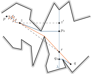
Figure 3: The shortest path $\pi(p,q)$ crosses $\lambda$ at $r$. The difference in length between the direct path from $z$ to $r$ and the path through $p_{\lambda}$ can be bounded by considering the triangle $\mathcal{T}=(z,z^{\prime},r)$.

Let $z$ be the point where the shortest paths from $p$ to $p_{\lambda}$ and $r$ separate. See Figure 3 for an illustration. Consider the right triangle $\mathcal{T}=(z,z^{\prime},r)$, where $z^{\prime}$ is the intersection point of the line perpendicular to $\lambda$ through $z$ and the line containing $\lambda$. Note that $z^{\prime}$ does not necessarily lie within $P$. For this triangle we have that

$$|zr|\geq\frac{\sqrt{2}}{2}(|zz^{\prime}|+|z^{\prime}r|).$$ (3)

Next, we show that the path from $z$ to $p_{\lambda}$ is a $y$-monotone convex polygonal chain ending at or below $z^{\prime}$. Consider the vertical ray through $z$ upwards to the polygon boundary. We call the part of $\partial P$ between where the ray hits $\partial P$ and $\lambda$ the top part of $\partial P$. Similarly, for a downwards ray, we define the bottom part of $\partial P$. There are no vertices on $\pi(z,p_{\lambda})$ from the bottom part of $\partial P$, because such a vertex would then also occur on the shortest path to $r$. This is in contradiction with the definition of $z$. If $z$ sees $z^{\prime}$, then $p_{\lambda}=z^{\prime}$, otherwise the chain must bend at one or more vertices of the top part of $\partial P$, and thus lie below $z^{\prime}$. It follows that $\pi(z,p_{\lambda})$ is contained within $\mathcal{T}$. Similarly, we conclude that $\pi(z,r)$ is contained within $\mathcal{T}$. Additionally, this gives us that $d(z,p_{\lambda})\leq|zz^{\prime}|+|z^{\prime}p_{\lambda}|$, and $d(z,r)\geq|zr|$. Together with Equation (3) this yields $d(z,p_{\lambda})+|p_{\lambda}r|\leq|zz^{\prime}|+|z^{\prime}r|\leq\sqrt{2}|zr|\leq\sqrt{2}d(z,r)$. And thus

$$d(p,p_{\lambda})+|p_{\lambda}r|=d(p,z)+d(z,p_{\lambda})+|p_{\lambda}r|\leq d(p,z)+\sqrt{2}d(z,r)\leq\sqrt{2}d(p,r).$$

Symmetrically, we find for $q$ that $d(q,q_{\lambda})+|q_{\lambda}r|\leq\sqrt{2}d(q,r)$. From this, together with Equation (2), we conclude that $d_{\mathcal{G}}(p,q)\leq t\left(\sqrt{2}d(p,r)+\sqrt{2}d(r,q)\right)=\sqrt{2}td(p,q)$.

Applying Lemma 3.1 to the spanner of Section 2 yields a $2\sqrt{2}$-spanner of size $O(n\log^{2}n)$.

3.1.1 A refinement to obtain a $(t+\varepsilon)$-spanner

Abam et al. [3] refine their spanner construction to obtain a $(2+\varepsilon)$-spanner for any constant $\varepsilon>0$. In the following lemma, we apply their refinement to the construction of the spanner proposed in Section 3.1 and obtain a $(t+\varepsilon)$-spanner. For the rest of the paper, we generally discuss the results based on the simple spanner from Section 3.1, as this is somewhat easier to follow, and apply the refinement only in the final results.

Lemma 3.3.

Using any 1-dimensional additively weighted $t$-spanner of size $O(n\log n)$, we can construct a $(t+\varepsilon)$-spanner for a set $S$ of $n$ point sites that lie in a simple polygon $P$ of size $O(c_{\varepsilon}n\log^{2}n)$, where $c_{\varepsilon,t}$ is a constant depending on $\varepsilon$ and $t$. The number of sites used to construct the 1-dimensional spanner is $O(c_{\varepsilon,t}n)$.

Proof 3.4.

In the refined construction, instead of adding only a single point $p_{\lambda}$ to $S_{\lambda}$ for each site $p$, we additionally add a collection of $O(1/\delta^{2})$ points on $\lambda$ “close” to $p_{\lambda}$ to $S_{\lambda}$, where $\delta$ is a constant depending on $\varepsilon$. These additional points all lie within distance $(1+2/\delta)\cdot d(p,p_{\lambda})$ of $p_{\lambda}$. The points are roughly equally spaced on the line segment within this distance. To be precise, the segment is partitioned into $O(1/\delta^{2})$ pieces of length $\delta\cdot d(p,p_{\lambda})$, and for each piece $i$ the point $p_{\lambda}^{(i)}$ closest to $p$ is added to $S_{\lambda}$. The weight of each point is again chosen as the geodesic distance to $p$. The 1-dimensional spanner(s) $\mathcal{G}_{\lambda}$ is then computed on this larger set $S_{\lambda}$. For each edge $(p_{\lambda}^{(i)},q_{\lambda}^{(j)})$ in $\mathcal{G}_{\lambda}$, we again add the edge $(p,q)$ to the final spanner $\mathcal{G}$.

Abam et al.prove that for each $p,q\in S$, there are points $p_{\lambda}^{(i)},q_{\lambda}^{(j)}\in S_{\lambda}$ such that $d_{w}(p_{\lambda}^{(i)},t_{\lambda}^{(j)})\leq(1+\delta)\cdot d(p,q)$. As $\mathcal{G}_{\lambda}$ is a $t$-spanner for $S_{\lambda}$, choosing $\delta=\varepsilon/t$ implies that $d_{\mathcal{G}}(p,q)\leq t\cdot d_{w}(p_{\lambda}^{(i)},t_{\lambda}^{(j)})\leq t(1+\delta)d(p,q)=(t+\varepsilon)d(p,q)$. In other words, $\mathcal{G}$ is a $(t+\varepsilon)$-spanner of $S$. Note that the number of edges in the spanner has increased because we use $O(n/\delta^{2})$ instead of $O(n)$ points to compute the 1-dimensional spanner. This results in a spanner of size $O(c_{\varepsilon,t}n\log^{2}n)$, where $c_{\varepsilon,t}=O(t^{2}/\varepsilon^{2})$ is a constant depending on $\varepsilon$.

3.2 Low complexity geodesic spanners

In general, a geodesic spanner $\mathcal{G}=(S,E)$ in a simple polygon with $m$ vertices may have complexity $O(m|E|)$. It is easy to see that the $2\sqrt{2}$-spanner of Section 3.1 can have complexity $\Omega(nm)$, just like the spanners in [3]. As one of the sites, $c$, is connected to all other sites, the polygon in Figure 4 provides this lower bound. The construction in Figure 4 even shows that the same lower bound holds for the complexity of any $(3-\epsilon)$-spanner. Additionally, the following theorem implies a trade-off between the spanning ratio and the spanner complexity.

Theorem 3.5.

For any constant $\varepsilon\in(0,1)$ and integer constant $t\geq 2$, there exists a set of $n$ point sites in a simple polygon $P$ with $m=\Omega(n)$ vertices for which any geodesic $(t-\varepsilon)$-spanner has complexity $\Omega(mn^{1/(t-1)})$.

The proofs of these lower bounds are in Section 6. Next, we present a spanner that almost matches this bound. We first present a $4\sqrt{2}$-spanner of bounded complexity, and then generalize the approach to obtain a $(2k+\varepsilon)$-spanner of complexity $O(mn^{1/k}+n\log^{2}n)$, for any integer $k\geq 2$.

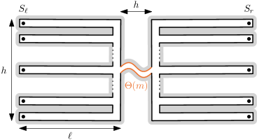
Figure 4: Any $(3-\varepsilon)$-spanner in a simple polygon with $m$ vertices may have complexity $\Omega(nm)$.

3.2.1 A $4\sqrt{2}$-spanner of complexity $O(m\sqrt{n}+n\log^{2}n)$

To improve the complexity of the geodesic spanner, we adapt our construction for the additively weighted spanner $\mathcal{G}_{\lambda}$ as follows. After finding the site $c_{\lambda}\in S_{\lambda}$ for which $d_{w}(c_{\lambda},O)$ is minimal, we do not add all edges $(p_{\lambda},c_{\lambda})$, $p_{\lambda}\in S_{\lambda}$, to $\mathcal{G}_{\lambda}$. Instead, we form groups of sites whose original sites (before projection) are “close” to each other in $P$. For each group $S_{i}$, we add all edges $(p_{\lambda},c_{i,\lambda})$, $p_{\lambda}\in S_{i}$, to $\mathcal{G}_{\lambda}$, where $c_{i,\lambda}$ is the site in $S_{i}$ for which $d_{w}(c_{i,\lambda},O)$ is minimal. Finally, we add all edges $(c_{i,\lambda},c_{\lambda})$ to $\mathcal{G}_{\lambda}$.

To make sure the complexity of our spanner does not become too large, we must choose the groups in such a way that the edges in our spanner do not cross “bad” parts of the polygon too often. We achieve this by making groups of roughly equal size, where shortest paths within each group $S_{i}$ are contained within a region $R_{i}$ that is (almost) disjoint from the regions $R_{j}$ of other groups. We first show how to solve a recursion that is later used to bound the complexity of the spanner. The subsequent lemma formally states the properties that we require of our groups, and bounds the complexity of such a spanner.

Lemma 3.6.

The recursion $T(n,m)=T(n/2,m_{1})+T(n/2,m_{2})+O(mn^{1/k}+n\log^{c_{1}}n)$, where $m_{1}+m_{2}=m+c_{2}$ and $c_{1},c_{2}$ integer constants, solves to $T(n)=O(mn^{1/k}+n\log^{c_{1}+1}n)$.

Proof 3.7.

We will write the recursion as a sum over all levels $i$ and all subproblems $j$ at each level. Because $n$ is halved in each level, the recursion has $O(\log n)$ levels. There are $2^{i}$ subproblems at level $i$ of the recursion.

Let $m_{i,j}$ denote the $m$ value used in subproblem $j$ of level $i$. We consider the sum of the $m$ values over all subproblems at level $i$ which we denote by $M_{i}$, so $M_{i}=\sum_{j=0}^{2^{i}}m_{i,j}$. We prove by induction that $M_{i}=m+c_{2}\cdot(2^{i}-1)$ for any $i\geq 1$. For $i=1$ this states that $M_{1}=m+c_{2}\cdot(2^{1}-1)=m+c_{2}$, which is equivalent to $m_{1}+m_{2}=m+c_{2}$. Suppose that the hypothesis $M_{i}=m+c_{2}\cdot(2^{i}-1)$ holds for $i=k$. The $2^{k+1}$ subproblems at level $k+1$ consist of $2^{k+1}/2=2^{k}$ pairs of subproblems $(j_{1},j_{2})$, each generated by a subproblem $j$ at level $k$, for which $m_{k+1,j_{1}}+m_{k+1,j_{2}}=m_{k,j}+c_{2}$. We can thus find $M_{k+1}$ by summing over these pairs. So, $M_{k+1}=\sum_{(j_{1},j_{2})}(m_{k,j}+c_{2})=M_{k}+c_{2}\cdot 2^{k}=m+c_{2}\cdot(2^{k}-1)+c_{2}\cdot 2^{k}=m+c_{2}\cdot(2^{k+1}-1)$.

We are now ready to formulate the recursion as a summation. For simplicity we use that $M_{i}\leq m+c_{2}2^{i}$.

$$T(n,m) =\sum_{i=0}^{O(\log n)}\sum_{j=0}^{2^{i}}\left(m_{i,j}\left(\frac{n}{2^{i}}\right)^{1/k}+\frac{n}{2^{i}}\log^{c_{1}}\left(\frac{n}{2^{i}}\right)\right)$$

$$=\sum_{i=0}^{O(\log n)}\sum_{j=0}^{2^{i}}m_{i,j}\left(\frac{n}{2^{i}}\right)^{1/k}+\sum_{i=0}^{O(\log n)}\sum_{j=0}^{2^{i}}\frac{n}{2^{i}}\log^{c_{1}}\left(\frac{n}{2^{i}}\right)$$

$$=\sum_{i=0}^{O(\log n)}\left(\frac{n}{2^{i}}\right)^{1/k}\sum_{j=0}^{2^{i}}m_{i,j}+O(n\log^{c_{1}+1}n)$$

$$\leq\sum_{i=0}^{O(\log n)}\left(\frac{n}{2^{i}}\right)^{1/k}(m+c_{2}2^{i})+O(n\log^{c_{1}+1}n)$$

$$=mn^{1/k}\sum_{i=0}^{O(\log n)}\frac{1}{2^{i/k}}+c_{2}n^{1/k}\sum_{i=0}^{O(\log n)}2^{(1-1/k)i}+O(n\log^{c_{1}+1}n)$$

$$=O(mn^{1/k})+c_{2}n^{1/k}\cdot O(n^{1-1/k})+O(n\log^{c_{1}+1}n)$$

$$=O(mn^{1/k}+n\log^{c_{1}+1}n).$$

Lemma 3.8.

If the groups adhere to the following properties, then $\mathcal{G}$ has $O(m\sqrt{n}+n\log^{2}n)$ complexity:

1. each group contains $\Theta(\sqrt{n})$ sites, and

2. each vertex of $P$ is only used by shortest paths within $O(1)$ groups.

Proof 3.9.

We will first prove the complexity of the edges in one level of the 1-dimensional spanner is $O(m\sqrt{n}+n)$. Two types of edges are added to the spanner: (a) edges from some $c_{i}$ to $c$, and (b) edges from some $p\in S_{i}$ to $c_{i}$. According to property 1, there are $\Theta(\sqrt{n})$ groups, and thus $\Theta(\sqrt{n})$ type (a) edges, that each have a complexity of $O(m)$. Thus the total complexity of these edges is $O(m\sqrt{n})$. Let $r_{i}$ be the maximum complexity of a shortest path between any two sites in $S_{i}$ and let $V_{i}$ be the set of vertices this path visits. Property 2 states that for any $v\in V_{i}$ it holds that $|\{j\mid v\in V_{j}\}|=O(1)$, which implies that $\sum_{i}r_{i}=O(m)$. The complexity of all type (b) edges is thus $O(n)+\sum_{i}r_{i}O(\sqrt{n})=O(m\sqrt{n}+n)$.

Next, we show that in both recursions, the 1-dimensional recursion and the recursion on $P_{\ell}$ and $P_{r}$, not only the number of sites, but also the complexity of the polygon is divided over the two subproblems. Splitting the sites into left and right of $O$ corresponds to splitting the polygon horizontally at $O$: all sites left (right) of $O$ in the 1-dimensional space lie in the part of the polygon below (above) this horizontal line segment. Thus, shortest paths between sites left of $O$ use part of the polygon that is disjoint from the shortest paths between the sites right of $O$. This means that for two subproblems we have that $m_{1}+m_{2}=m$, where $m_{i}$ denotes the maximum complexity of a path in subproblem $i$. The recursion for the complexity is now given by

$$T(n,m)=T(n/2,m_{1})+T(n/2,m_{2})+O(m\sqrt{n}+n)\text{, with }m_{1}+m_{2}=m.$$

According to Lemma 3.6 this solves to $T(n)=O(m\sqrt{n}+n\log n)$.

Similarly, the split by $\lambda$ divides the polygon into two subpolygons, while adding at most two new vertices. As all vertices, except for the endpoints of $\lambda$, are in $P_{\ell}$ or $P_{r}$ (not both), the total complexity of both subpolygons is at most $m+4$. We obtain the following recursion

$$T(n,m)=T(n/2,m_{1})+T(n/2,m_{2})+O(m\sqrt{n}+n\log n)\text{, with }m_{1}+m_{2}=m+4.$$

Lemma 3.6 again states this solves to $T(n)=O(m\sqrt{n}+n\log^{2}n)$.

To form groups that adhere to these two properties, we consider the shortest path tree $\mathit{SPT}_{c}$ of $c$: the union of all shortest paths from $c$ to the vertices of $P$. We include the sites $p\in S\setminus\{c\}$ as leaves in $\mathit{SPT}_{c}$ as children of their apex, i.e., the last vertex on $\pi(c,p)$. This gives rise to an ordering of the sites in $S$, and thus of the weighted sites in $S_{\lambda}$, based on the in-order traversal of the tree. We assign the first $\lceil\sqrt{n}\rceil$ sites to $S_{1}$, the second $\lceil\sqrt{n}\rceil$ to $S_{2}$, etc. See Figure 5.

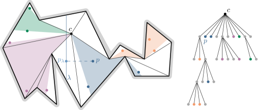
Figure 5: The shortest path tree of $c$. The polygon vertices are grey in the tree. Each group $S_{i}$ has an associated polygonal region $R_{i}$ in $P$.

Clearly these groups adhere to property 1. Proving that they also adhere to property 2 is more involved. For each group $S_{i}$, consider the minimal subtree $\mathcal{T}_{i}$ of $\mathit{SPT}_{c}$ containing all $p\in S_{i}$. $\mathcal{T}_{i}$ defines a polygonal region $R_{i}$ in $P$ as follows. Refer to Figure 5 for an illustration. Let $v_{i}$ be the root of $\mathcal{T}_{i}$. Consider the shortest path $\pi(v_{i},a)$, where $a$ is the first site of $S_{i}$ in $\mathcal{T}_{i}$ by the ordering used before. Let $\pi_{a}$ be the path obtained from $\pi(v_{i},a)$ by extending the last segment of $\pi(v_{i},a)$ to the boundary of $P$. Similarly, let $\pi_{b}$ be such a path for the last site of $S_{i}$ in $\mathcal{T}_{i}$. We take $R_{i}$ to be the region in $P$ rooted at $v_{i}$ and bounded by $\pi_{a}$, $\pi_{b}$, and some part of the boundary of $P$, that contains the sites in $S_{i}$. In case $v_{i}$ is $c$, we split $R_{i}$ into two regions $R_{j}$ and $R_{k}$, such that the angle of each of these regions at $c$ is at most $\pi$. The set $S_{i}$ is then also split into two sets $S_{j}$ and $S_{k}$ accordingly. The following three lemmas on $R_{i}$ and $\mathcal{T}_{i}$ together imply that the groups adhere to property 2.

Lemma 3.10.

Only vertices of $P$ that are in $\mathcal{T}_{i}$ can occur in $R_{i}$.

Proof 3.11.

Let $v$ be a vertex in $R_{i}$. The paths $\pi_{a}$ and $\pi_{b}$ are shortest paths from the polygon boundary to $v_{i}$. Additionally, we can extend these paths with $\pi(v_{i},c)$ to obtain shortest paths to the site $c$. The shortest path from $v$ to $c$ cannot intersect either of these shortest paths twice, thus $v$ is in $\mathcal{T}_{i}$.

Lemma 3.12.

All shortest paths between sites in $S_{i}$ are contained within $R_{i}$.

Proof 3.13.

Suppose there is a shortest path $\pi(p,q)$, $p_{\lambda},q_{\lambda}\in S_{i}$, that is not contained within $R_{i}$. Then $\pi(p,q)$ must exit $R_{i}$ through $\pi_{a}$ and enter again through $\pi_{b}$, or the other way around. The path thus goes around $v_{i}$. Consider a line through $v_{i}$ that does not pass through the interior of $R_{i}$. Note that this exists because $v_{i}$ is not a reflex vertex of $R_{i}$. As $P$ is a simple polygon, the line must intersect $\pi(p,q)$ twice. This provides a shortcut of the shortest path by following along the line, which is a contradiction.

Lemma 3.14.

Any vertex $v\in\mathit{SPT}_{c}$ occurs in at most two trees $\mathcal{T}_{i}$ and $\mathcal{T}_{j}$ as a non-root node.

Proof 3.15.

Let $v\in\mathcal{T}$, and $\mathcal{T}(v)$ be the subtree rooted at $v$. Suppose $v$ is a non-root node of three trees $\mathcal{T}_{i}$, $\mathcal{T}_{j}$, and $\mathcal{T}_{k}$, $i<j<k$. Then there must be three sites $p_{i}\in S_{i}$, $p_{j}\in S_{j}$, and $p_{k}\in S_{k}$ in $\mathcal{T}(v)$. As our groups occur in order, we know $p_{i}$ is before $p_{j}$, and $p_{j}$ is before $p_{k}$ in the in-order traversal of $\mathit{SPT}_{c}$. Let $p$ be the parent of $v$. As $v$ is a non-root node of each of the subtrees, we know that $p$ is in $\mathcal{T}_{i}$, $\mathcal{T}_{j}$, and $\mathcal{T}_{k}$ as well. This implies that there must be a site $p_{j}^{\prime}\in S_{j}$ in $\mathcal{T}(p)\setminus\mathcal{T}(v)$. If $p_{j}^{\prime}$ is before $p_{j}$, then $p_{j}^{\prime}$ is also before $p_{i}$, because $p_{j}^{\prime}\notin\mathcal{T}(v)$. This implies that $p_{i}$ is in $S_{j}$, because it lies between $p_{j}^{\prime}\in S_{j}$ and $p_{j}\in S_{j}$, which is a contradiction. If $p_{j}^{\prime}$ is after $p_{j}$, then the same reasoning implies $p_{k}\in S_{j}$, which is also a contradiction.

Note that the root $r$ of $\mathcal{T}_{i}$ is never used in a shortest path between sites in $S_{i}$, because $r$ cannot be a reflex vertex of $R_{i}$. Consequently, Lemma 3.8 states that the spanner has complexity $O(m\sqrt{n}+n\log^{2}n)$.

Lemma 3.16.

The graph $\mathcal{G}$ is a geodesic $4\sqrt{2}$-spanner of size $O(n\log^{2}n)$.

Proof 3.17.

We prove the 1-dimensional spanner $\mathcal{G}_{\lambda}$ is a 4-spanner with $O(n\log n)$ edges. Together with Lemma 3.1, this directly implies $\mathcal{G}$ is a $4\sqrt{2}$-spanner with $O(n\log^{2}n)$ edges.

In each level of the recursion, we still add only a single edge for each site. Thus, the total number of edges is $O(n\log n)$. Again, consider two sites $p_{\lambda},q_{\lambda}\in S_{\lambda}$, and let $c_{\lambda}$ be the chosen center point at the level where $p_{\lambda}$ and $q_{\lambda}$ are separated by $O$. Let $S_{i}$ be the group of $p_{\lambda}$ and $S_{j}$ the group of $q_{\lambda}$. Both the edges $(p_{\lambda},c_{i,\lambda})$ and $(c_{i,\lambda},c_{\lambda})$ are in $\mathcal{G}_{\lambda}$, similarly for $q_{\lambda}$. We thus have a path $p_{\lambda}\to c_{i,\lambda}\to c_{\lambda}\to c_{j,\lambda}\to q_{\lambda}$ in $\mathcal{G}_{\lambda}$. Using that $d_{w}(p_{\lambda},c_{i,\lambda})\leq d_{w}(p_{\lambda},O)+d_{w}(c_{i,\lambda},O)$, because of the triangle inequality, and $d_{w}(c_{i,\lambda},O)\leq d_{w}(p_{\lambda},O)$, we find:

$$d_{\mathcal{G}_{\lambda}}(p_{\lambda},q_{\lambda}) =d_{w}(p_{\lambda},c_{i,\lambda})+d_{w}(c_{i,\lambda},c_{\lambda})+d_{w}(c_{\lambda},c_{j,\lambda})+d_{w}(c_{j,\lambda},q_{\lambda})$$

$$\leq d_{w}(p_{\lambda},O)+2d_{w}(c_{i,\lambda},O)+2d_{w}(c_{\lambda},O)+2d_{w}(c_{j,\lambda},O)+d_{w}(q_{\lambda},O)$$

$$\leq 4d_{w}(p_{\lambda},O)+4d_{w}(q_{\lambda},O)$$

$$=4d_{w}(p_{\lambda},q_{\lambda})$$

3.2.2 A $(2k+\varepsilon)$-spanner of complexity $O(mn^{1/k}+n\log^{2}n)$

We first sketch how to generalize the approach of Section 3.2.1 to obtain a spanner with a trade-off between the (constant) spanning ratio and complexity, and then formally prove the result in Lemma 3.18. Fix $N=n^{1/k}$, for some integer constant $k\geq 1$. Instead of $\Theta(\sqrt{n})$ groups, we create $\Theta(N)$ groups. For each of these groups we select a center, and then partition the groups further recursively. By connecting each center to its parent center, we obtain a tree of height $k$. This results in a spanning ratio of $2\sqrt{2}k$. Using the refinement discussed in Lemma 3.3, we even obtain a $(2k+\varepsilon)$-spanner.

Lemma 3.18.

For any constant $\varepsilon>0$ and integer constant $k\geq 1$, there exists a geodesic $(2k+\varepsilon)$-spanner of size $O(c_{\varepsilon,k}n\log^{2}n)$ and complexity $O(c_{\varepsilon,k}(mn^{1/k}+n\log^{2}n))$, where $c_{\varepsilon,k}$ is a constant depending only on $\varepsilon$ and $k$.

Proof 3.19.

We prove that the 1-dimensional spanner we just sketched is a $2k$-spanner of complexity $O(mn^{1/k}+n\log n)$ with $O(n\log n)$ edges. Lemma 3.1, together with Lemma 3.6, then implies that $\mathcal{G}$ is a geodesic $2\sqrt{2}k$-spanner of complexity $O(mn^{1/k}+n\log^{2}n)$ and size $O(n\log^{2}n)$. The refinement discussed next in Lemma 3.3 can also be applied to this spanner, which yields a $(2k+\varepsilon)$-spanner. However, this slightly increases the spanner complexity to $O(c_{\varepsilon,k}(mn^{1/k}+n\log^{2}n))$, where $c_{\varepsilon,k}$ is a constant depending on $\varepsilon$ and $k$, see Lemma 3.3. We first describe the 1-dimensional spanner in more detail, then analyze its complexity, and finally analyze its size and spanning ratio.

Fix $N=n^{1/k}$. When building a single level of the 1-dimensional spanner $\mathcal{G}_{\lambda}$, instead of $\Theta(\sqrt{n})$ groups of size $\Theta(\sqrt{n})$, we create $\Theta(N)$ groups of size $\Theta(n^{1-1/k})$, based on the shortest path tree of $c$, for some integer constant $k\geq 1$. After selecting a center $c_{i}$ for each group $S_{i}$, we recursively split the groups further based on the shortest path trees of the new centers $c_{i}$, until we reach groups of size one. For each group $S_{i}$ at level $j$ of this recursion, a center $c^{(j)}_{i}$ is selected as the site in $S_{i}$ for which $d_{w}(c^{(j)}_{i},O)$ is minimal. We add an edge from each $c^{(j)}_{i}$ to its parent $c^{(j-1)}_{i^{\prime}}$. The final tree $T$ obtained this way has height $k$.

Let $r^{(j)}_{i}$ be the number of vertices in $R^{(j)}_{i}$ of a group $S_{i}$ at level $j$, where $R_{i}^{(j)}$ is defined as in Section 3.2.1. In other words, $r^{(j)}_{i}$ is the maximum complexity of a shortest path between two sites in $S_{i}$ at level $j$, as in the proof of Lemma 3.8. Let $S_{1}^{(j)},...,S_{O(N)}^{(j)}$ be the subgroups of some group $S_{i^{\prime}}^{(j-1)}$. Then the corresponding regions $R_{1}^{(j)},...,R_{O(N)}^{(j)}$ partition $R^{(j-1)}_{i^{\prime}}$, and Lemma 3.14 implies that a vertex of $R_{O(N)}^{(j)}$ can be in at most two of the smaller regions. Thus, we still have that $\sum_{i}r^{(j)}_{i}=O(m)$. This implies that the complexity all edges from level $j$ to $j-1$ is $O(mn^{1/k}+n)$. As $T$ has height $O(k)$, the total complexity of the edges in $T$ is also $O(mn^{1/k}+n)$. Lemma 3.6 implies that this results in a 1-dimensional spanner of complexity $O(mn^{1/k}+n\log n)$.

In a single level of the recursion to build the 1-dimensional spanner $\mathcal{G}_{\lambda}$, only one edge is added for each site, namely to its parent in the tree. We thus still add $O(n)$ edges in each level of the recursion, and $O(n\log n)$ edges in total.

Consider two sites $p,q\in S_{\lambda}$, and let $c$ be the chosen center point at the level where $p$ and $q$ are separated by $O$. The spanning ratio of the 1-dimensional spanner is determined by the number of sites we visit on a path from $p\in S_{\ell}$ to $q\in S_{r}$. Observe that the height of the tree $T$ is $k$. We assume w.l.o.g. that the path from $p$ to $q$ is as long as possible, i.e. visits $2k-1$ vertices. In a slight abuse of notation, we denote by $c^{(j)}_{p}$ the centers on the path in $T$ from $p$ to the root $c$. Then there is a path $p\to c^{(k-1)}_{p}\to c^{(k-2)}_{p}\to...\to c^{(0)}(=c)\to...\to c^{(k-2)}_{q}+c^{(k-1)}_{q}\to q$. Using that $d_{w}(c^{(j)}_{p},c^{(j+1)}_{p})\leq d_{w}(c^{(j)}_{p},O)+d_{w}(c^{(j+1)}_{p},O)$ and that $d_{w}(c^{(j)}_{p},O)\leq d_{w}(p,O)$, we find:

$$\begin{split}d_{\mathcal{G}_{\lambda}}(p,q)&=d_{w}(p,c^{(k-1)}_{p})+\sum_{j=0}^{k-2}d_{w}(c^{(j+1)}_{p},c^{(j)}_{p})+\sum_{j=0}^{k-2}d_{w}(c^{(j)}_{q},c^{(j+1)}_{q})+d_{w}(c^{(k-1)}_{q},q)\\ &\leq d_{w}(p,O)+2\sum_{j=1}^{k-1}d_{w}(c^{(j)}_{p},O)+2d_{w}(c,O)+2\sum_{j=1}^{k-1}d_{w}(c^{(j)}_{q},O)+d_{w}(q,O)\\ &\leq d_{w}(p,O)+2(k-1)d_{w}(p,O)+2d_{w}(c,O)+2(k-1)d_{w}(q,O)+d_{w}(q,O)\\ &\leq 2k(d_{w}(p,O)+d_{w}(q,O))\\ &=2kd_{w}(p,q).\end{split}$$

Thus the spanning ratio of the 1-dimensional spanner is $2k$.

3.3 Construction algorithm

In this section we propose an algorithm to construct the spanners of Section 3.2. The following gives a general overview of the algorithm, which computes a $2\sqrt{2}k$-spanner in $O(n\log^{2}n+m\log n)$ time. In the rest of this section we will discuss the steps in more detail.

1. Preprocess $P$ for efficient shortest path queries and build both the vertical decomposition $\mathcal{VD}$ and horizontal decomposition $\mathcal{HD}$ of $P$.

2. For each $p\in S$, find the trapezoid in $\mathcal{VD}$ and $\mathcal{HD}$ that contains $p$. For each trapezoid $\nabla\in\mathcal{VD}$, store the number of sites of $S$ that lies in $\nabla$ and sort these sites on their $x$-coordinate.

3. Recursively compute a spanner on the sites $S$ in $P$:

   1. Find a vertical chord $\lambda$ of $P$ such that $\lambda$ partitions $P$ into two polygons $P_{\ell}$ and $P_{r}$, and each subpolygon contains at most $2n/3$ sites using the algorithm of Lemma 3.20.

   2. For each $p\in S$, find the point $p_{\lambda}$ on $\lambda$ and its weight using the algorithm of Lemma 3.22, and add this point to $S_{\lambda}$.

   3. Compute an additively weighted 1-dimensional spanner $\mathcal{G}_{\lambda}$ on the set $S_{\lambda}$ using the algorithm of Lemma 3.24 or Lemma 3.26.

   4. For every edge $(p_{\lambda},q_{\lambda})\in E_{\lambda}$ add the edge $(p,q)$ to $\mathcal{G}$.

   5. Recursively compute spanners for $S_{\ell}$ in $P_{\ell}$ and $S_{r}$ in $P_{r}$.

In step 1, we preprocess the polygon in $O(m)$ time such that the distance between any two points $p,q\in P$ can be computed in $O(\log m)$ time [15, 23]. We also build the horizontal and vertical decompositions of $P$, and a corresponding point location data structure, as a preprocessing step in $O(m)$ time [15, 28]. We then perform a point location query for each site $p\in S$ in $O(n\log m)$ time in step 2 and sort the sites within each trapezoid in $O(n\log n)$ time in total. The following lemma describes the algorithm to compute a vertical chord that partitions $P$ into two subpolygons such that each of them contains roughly half of the sites in $S$. It is based on the algorithm of Bose et al. [7] that finds such a chord without the constraint that it should be vertical. Because of this constraint, we use the vertical decomposition of $P$ instead of a triangulation in our algorithm.

Lemma 3.20.

In $O(n+m)$ time, we can find a vertical chord of $P$ that partitions $P$ into two subpolygons $P_{\ell}$ and $P_{r}$, such that each subpolygon contains at most $2n/3$ sites of $S$.

Proof 3.21.

Consider the dual tree of the vertical decomposition $\mathcal{VD}$. Because our polygon vertices have distinct $x$- and $y$-coordinates, the maximum degree of any node in the tree is four; at most two neighbors to the right and two to the left of the trapezoid. We select an arbitrary node $r$ as root of the tree. For each node $v$, we compute $c(v)$: the number of sites in $S$ that lie in some trapezoid of the subtree rooted at $v$. These values can be computed in linear time (in the size of the polygon) using a bottom-up approach, because we already know the number of sites that lie in each trapezoid.

Let $v$ be an arbitrary node in the tree and $\nabla_{v}$ the corresponding trapezoid. We first show that there is a vertical segment contained in $\nabla_{v}$ that partitions the polygon such that each subpolygon contains at most $2/3$ of the sites if

1. $n/3\leq c(v)\leq 2n/3$, or

2. $\nabla_{v}$ contains at least $2n/3$ sites, or

3. for each child $w$ of $v$ we have $c(w)<n/3$, and $c(v)>2n/3$.

In case 1, we choose $\lambda$ as the vertical segment between the trapezoid of $v$ and its parent. In case 2, we choose $\lambda$ as a segment for which exactly $n/3$ sites in $\nabla_{v}$ lie left of $\lambda$. As $\nabla_{v}$ contains more than $2n/3$ sites, at most $n/3$ sites lie outside of $\nabla_{v}$, thus $P_{\ell}$ contains between $n/3$ and $2n/3$ sites.

In case 3, we choose $\lambda$ to lie within $\nabla_{v}$. Note that $v$ must have at least two children, otherwise $\Delta_{v}$ would contain at least $2n/3-n/3=n/3$ sites, thus we would be in case 1 or case 2. Assume that $\nabla_{p(v)}$ lies right of $\nabla_{v}$, where $p(v)$ denotes the parent of $v$. We consider the two children $u,w$ for which the trapezoids lie left of $\nabla_{v}$, see Figure 6. When there is only one such site $u$, we consider $c(w)=0$. It holds that $c(u)+c(w)<2n/3$. We choose $\lambda$ such that $\max(0,n/3-c(u)-c(w))$ sites in $\nabla_{v}$ lie left of $\lambda$. Thus $P_{\ell}$ contains between $n/3$ and $2n/3$ sites of $S$. Similarly, we consider the children on the right when $\nabla_{p(v)}$ lies left of $\nabla_{v}$.

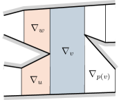
Figure 6: The trapezoid $\nabla_{v}$ has parent $\nabla_{p(v)}$ and relevant children $\nabla_{u}$ and $\nabla_{w}$.

We now show that if none of the above conditions hold, there is a path in the tree to a node for which one of these conditions holds. If none of the above conditions hold, then either $c(v)<n/3$, or $c(v)>2n/3$ and there is a child $w$ of $v$ with $c(w)\geq n/3$. In the first case, we consider the node $p(v)$, in the second case we consider the node $w$ with $c(w)\geq n/3$. By continuing like this, a path in the tree is formed. If the path ends up in $r$, it must hold that $c(r)>2n/3$, and thus condition 2 holds. If the path ends up in a leaf node, then either condition 1 or 2 must hold for the leaf node.

This proves not only that there exists such a vertical segment, but also provides a way to find such a segment. As the tree contains $O(m)$ nodes, we can find a trapezoid that can contain $\lambda$ in $O(m)$ time. We can separate the sites in a trapezoid by a vertical line segment such that exactly $x$ sites lie left of the segment in linear time. Thus, the algorithm runs in $O(n+m)$ time.

The following lemma states that we can find the projections $p_{\lambda}$ efficiently. The algorithm produces not only these projected sites, but also the shortest path tree $\mathit{SPT}_{\lambda}$ of $\lambda$.

Lemma 3.22.

We can compute the closest point $p_{\lambda}$ on $\lambda$ and $d(p,p_{\lambda})$ for all sites $p\in S$, and the shortest path tree $\mathit{SPT}_{\lambda}$, in $O(m+n\log m)$ time.

Proof 3.23.

Consider the horizontal decomposition $\mathcal{HD}$ of $P$ and its dual tree $T$. Let $x_{\lambda}$ denote the $x$-coordinate of the vertical line segment $\lambda$ and let $t$ be its top endpoint and $b$ its bottom endpoint. We choose the root $r$ of the tree as the trapezoid $\nabla_{r}$ for which $t\in\nabla_{r}$ and $\nabla_{r}\cap\lambda\neq\emptyset$. We color $T$ as follows, see Figure 7 for an example. Every node $v$ for which the corresponding trapezoid $\nabla_{v}$ contains the top or bottom endpoint of $\lambda$ is colored orange. Note that the root $r$ is thus colored orange. Every node $v$ for which $\nabla_{v}$ is crossed from top to bottom by $\lambda$ is colored blue. For every other node $v\in T$, consider its lowest ancestor $w$ that is colored either blue or orange. If $w$ is blue, then $v$ is colored green, if $w$ is orange, $v$ is colored purple. Next, we describe how to find $p_{\lambda}$ for a site $p=(x_{p},y_{p})\in\nabla_{v}$ for each color of $v$.

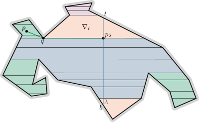
Figure 7: An example of the coloring of the horizontal decomposition in a simple polygon.

Blue: The horizontal line segment connecting $p$ and $\lambda$ is contained within $P$. So, $p_{\lambda}=(x_{\lambda},y_{p})$.

Orange: The shortest path to $\lambda$ is again a line segment. If $p$ lies above $t$ or below $b$, then $p_{\lambda}$ is $t$ or $b$, respectively. Otherwise, $p_{\lambda}=(x_{\lambda},y_{p})$.

Green: Let $w$ be the highest green ancestor of $v$ (possibly $v$ itself). Suppose that $\nabla_{w}$ lies above the trapezoid $\nabla_{p(w)}$ of its (blue) parent and $\nabla_{w}$ lies in $P_{\ell}$. Let $q$ be the bottom right corner of $\nabla_{w}$. Then $q_{\lambda}=(x_{\lambda},y_{q})$, as $q$ also lies in $\nabla_{p(w)}$. We will show that $p_{\lambda}=q_{\lambda}$. Suppose to the contrary that $p_{\lambda}\neq q_{\lambda}$. As $v$ is a descendant of $w$, any path from $p$ to $\lambda$ must intersect the bottom of $\nabla_{v}$. Let $q^{\prime}$ be the this intersection point. Because $q^{\prime}$ lies on the bottom boundary of $\nabla_{w}$, the horizontal line segment $q^{\prime}q_{\lambda}$ is contained within $P$ and thus $q^{\prime}_{\lambda}=q_{\lambda}$. Because $d(q^{\prime},q^{\prime}_{\lambda})=d(q^{\prime},q_{\lambda})<d(q^{\prime},p_{\lambda})$, subpath optimality implies that $d(p,q_{\lambda})<d(p,p_{\lambda})$, which is a contradiction. So $p_{\lambda}=q_{\lambda}$. Symmetrically, we can show a similar statement when $\nabla_{v}$ lies below $\nabla_{p(v)}$ and/or $\nabla_{v}$ lies in $P_{r}$.

Purple: Let $w$ be the highest purple ancestor of $v$. Assume that $\nabla_{p(w)}$ lies below $\nabla_{w}$. Note that the bottom segment of $\nabla_{w}$ lies above $t$. It follows that for all points $q$ on this segment we have $q_{\lambda}=t$. According to the same argument as for the green trapezoids, we thus have $p_{\lambda}=t$. Symmetrically, if $\nabla_{p(w)}$ lies above $\nabla_{w}$, then $p_{\lambda}=b$.

We can thus find $p_{\lambda}$ for all $p\in S$ as follows. We perform a depth first search on $T$ starting at $r$. When we visit a node $v$, we first determine its color in $O(1)$ time. Then for all $p\in\nabla_{v}$ we determine $p_{\lambda}$ as described before. Note that this can also be done in constant time, because for a green/purple node we already computed the projected sites for the parent trapezoid. This thus takes $O(m+n)$ time overall.

The shortest path tree $\mathit{SPT}_{\lambda}$ can now be computed as follows. All vertices of $P$ in a blue trapezoid are children of $\lambda$. At most four of these vertices lie on the boundary of the blue and green region (such as $q$ in Figure 7). For each such vertex $q$, we include the shortest path tree of $q$ restricted to its respective green region as a subtree of $q$. We include the shortest path trees of $t$ and $b$ restricted to the top and bottom orange and purple regions as a subtree of $\lambda$. Because the regions where we construct a shortest path trees are disjoint, we can compute all of these shortest path trees in $O(m)$ time [24]. Finally, for all $p\in S$ we compute $d(p,p_{\lambda})$ in $O(n\log m)$ time, and include each site in $\mathit{SPT}_{\lambda}$ as a child of their apex.

Lemma 3.24.

Given $\mathit{SPT}_{\lambda}$, we can construct a $4$-spanner $\mathcal{G}_{\lambda}$ on the additively weighted points $S_{\lambda}$, where the groups adhere to the properties of Lemma 3.8, in $O(n\log n+m)$ time.

Proof 3.25.

The $4$-spanner of Section 3.2.1 requires an additional step at each level of the recursion, namely the formation of $\Theta(\sqrt{n})$ groups. We first discuss the running time to construct a $4$-spanner when forming the groups as in Section 3.2.1, and then improve the running time by introducing a more efficient way to form the groups.

In Section 3.2.1, the groups are formed based on the shortest path tree of the site $c$. Building the shortest path tree, and a corresponding point location data structure, takes $O(m)$ time [24]. Then, we perform a point location query for each site to find its apex in the shortest path tree, and add the sites to the tree. These queries take $O(n\log m)$ time in total. We form groups based on the traversal of the tree. Note that we do not distinguish between sites with the same parent in the tree, as the tree $\mathcal{T}_{i}$ (and thus the region $R_{i}$) obtained contains the same vertices of $P$ regardless of the order of these sites. After obtaining the groups, we again add only $O(n)$ edges to the spanner. The overall running time of the algorithm is thus $O((m+n\log m)\log n)$.

This running time can be improved by using another approach to form the groups. To form groups that adhere to the properties of Lemma 3.8, and thus result in a spanner of the same complexity, we can use any partition of $P$ into regions $R_{i}$, as long $R_{i}$ as contains $\Theta(\sqrt{n})$ sites and $\sum_{i}r_{i}=O(m)$. Next, we describe how to form such groups efficiently using $\mathit{SPT}_{\lambda}$.

We first define an ordering on the sites. This is again based on the traversal of some shortest path tree. Instead of considering the shortest path tree of a point site, we consider the shortest path tree $\mathit{SPT}_{\lambda}$ of $\lambda$. Again, all sites in $S$ are included in this shortest path tree. Additionally, we split the node corresponding to $\lambda$ into a node for each distinct projection point on $\lambda$ (of the vertices and the sites) and add an edge between each pair of adjacent points, see Figure 8. We root the tree at the node corresponding to the bottom endpoint of $\lambda$. Whenever a node $t$ on $\lambda$ has multiple children, in other words, when multiple sites are projected to the same point $t$, our assumption that all $y$-coordinates are distinct ensures that all these sites lie either in $P_{\ell}$ or $P_{r}$.

The groups are formed based on the in-order traversal of this tree, which can be performed in $O(m+n)$ time. As before, the first $\lceil\sqrt{n}\rceil$ are in $S_{1}$, the second in $S_{2}$, etc. The groups thus adhere to the first property. Next, we show they also adhere to the second property.

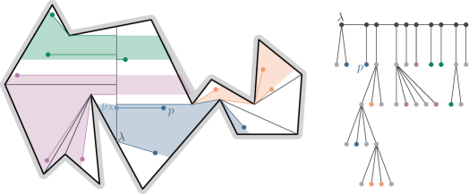
Figure 8: The shortest path tree $\mathit{SPT}_{\lambda}$ and associated polygonal region $R_{i}$ for each group $S_{i}$.

For each group $S_{i}$, we again consider the minimal subtree $\mathcal{T}_{i}$ of $\mathit{SPT}_{\lambda}$ containing all $p\in S_{i}$. $\mathcal{T}_{i}$ defines a region $R_{i}$ in $P$ as follows. Let $a$ be the first site of $S_{i}$ in $\mathcal{T}_{i}$ by the ordering used before. Assume that $a$ lies in $P_{\ell}$. We distinguish two cases: $a_{\lambda}\in\mathcal{T}_{i}$, or $a_{\lambda}\notin\mathcal{T}_{i}$. When $a_{\lambda}\in\mathcal{T}_{i}$, then let $\pi_{a}$ be the path obtained from $\pi(a_{\lambda},a)$ by extending the last segment to the boundary of $P$. Additionally, we extend $\pi_{a}$ into $P_{r}$ horizontally until we hit the polygon boundary. When $a_{\lambda}\notin\mathcal{T}_{i}$, consider the root $v_{i}$ of $\mathcal{T}_{i}$. Let $\pi_{a}$ be the path obtained from $\pi(v_{i},a)$ by extending the last segment of the path to the boundary of $P$. Similarly, let $\pi_{b}$ be such a path for the rightmost site of $S_{i}$ in $\mathcal{T}_{i}$. We take $R_{i}$ to be the region in $P$ bounded by $\pi_{a}$, $\pi_{b}$, and some part of the boundary of $P$ that contains the sites in $S_{i}$. See Figure 8. Note that, as before, only vertices of $P$ that are in $\mathcal{T}_{i}$ can occur in $R_{i}$. All shortest paths between sites in $S_{i}$ are contained within $R_{i}$. Just as for the shortest path tree of $c$, Lemma 3.14 implies that any vertex $v\in\mathit{SPT}_{\lambda}$ occurs in at most two trees $\mathcal{T}_{i}$ and $\mathcal{T}_{j}$ as a non-root vertex. We conclude that any vertex is used by shortest paths within at most two groups.

After splitting $\lambda$ at a point $O$, the tree $\mathit{SPT}_{\lambda}$ is also split into two trees $\mathcal{T}_{\ell}$ and $\mathcal{T}_{r}$ that contain exactly the sites in $S_{\ell}$ and $S_{r}$. We can thus reuse the ordering to form groups at each level of the recursion. This way, the total running time at a single level of the recursion is reduced to $O(n)$. The overall running time thus becomes $O(n\log n+m)$.

Lemma 3.26.

Given $\mathit{SPT}_{\lambda}$, we can construct a $2k$-spanner $\mathcal{G}_{\lambda}$ on the additively weighted points $S_{\lambda}$, where groups are formed as in Section 3.2.2, in $O(n\log n+m)$ time.

Proof 3.27.

To construct the 1-dimensional $2k$-spanner of Section 3.2.2, we can use the shortest path tree of $\lambda$ to form the groups as before. Note that we can select a center for each group after computing the groups, as including the center in the subgroups does not influence spanning ratio or complexity. After ordering the sites based on the in-order traversal of $\mathit{SPT}_{\lambda}$, we can build the tree of groups in linear time using a bottom up approach. As before, fix $N=n^{1/k}$. We first form the $\Theta(N^{k})$ lowest level groups, containing only a single site, and select a center for each group. Each group at level $i$ is created by merging $\Theta(N)$ groups at level $i-1$, based on the same ordering. We do not perform this merging explicitly, but for each group we select the site closest to $O$ of the merged level-($i-1$) centers as the center. Because our center property, being the closest to $O$, is decomposable, this indeed gives us the center of the entire group. This way, we can compute the edges added in one level of the recursion in linear time, so the running time remains $O(n\log n+m)$.

The total running time thus becomes $O((n(\log n+\log m)+m)\log n)=O(n\log^{2}n+m\log n)$. Here, we used that $n\log n\log m=O(n\log^{2}n)$ for $m<n^{2}$, and $n\log n\log m=O(m\log n)$ for $m\geq n^{2}$. By splitting the polygon alternately based on the sites and the polygon vertices, we can replace the final $O(\log n)$ factor by $O(\min(\log n,\log m))$.

When we apply the refinement of Lemma 3.3, step 3 is performed on $c_{\varepsilon,k}n$ sites, where $c_{\varepsilon,k}$ is a constant depending only on $\varepsilon$ and $k$, increasing the running time for this step by a factor $O(c_{\varepsilon,k})$. Together with Lemma 3.18, we obtain the following theorem.

Theorem 3.28.

Let $S$ be a set of $n$ point sites in a simple polygon $P$ with $m$ vertices, and let $k\geq 1$ be any integer constant. For any constant $\varepsilon>0$, we can build a geodesic $(2k+\varepsilon)$-spanner of size $O(c_{\varepsilon,k}n\log^{2}n)$ and complexity $O(c_{\varepsilon,k}(mn^{1/k}+n\log^{2}n))$ in $O(c_{\varepsilon,k}n\log^{2}n+m\log n+K)$ time, where $c_{\varepsilon,k}$ is a constant depending only on $\varepsilon$ and $k$, and $K$ is the output complexity.

4 Balanced shortest-path separators

Let $S$ be a set of $n$ point sites inside a polygonal domain $P$ with $m$ vertices. We denote by $\partial P$ and $\partial H$ the boundary of the outer polygon and the boundary of the holes, respectively. In this section, we develop an algorithm to partition the polygonal domain $P$ into two subdomains $P_{\ell}$ and $P_{r}$ such that roughly half of the sites in $S$ lie in $P_{\ell}$ and half in $P_{r}$. Additionally, we require that the curve bounding $P_{\ell}$ consists of at most three shortest paths and possibly part of $\partial P$ or $\partial H$.

In a polygonal domain, we cannot simply split the domain into two subdomains by a line segment, as we did to partition a simple polygon, because any line segment that appropriately partitions $S$ might intersect one or more holes. Even if we allow a shortest path between two points on $\partial P$ as our separator, it is not always possible to split the sites into sets $S_{\ell}$ and $S_{r}$ of roughly equal size. See Figure 9 for an example. We thus need another approach for subdividing the domain. We adapt the balanced shortest-path separator of Abam et al. [3] for this purpose.

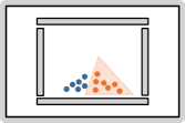
Figure 9: No shortest path between two points on the boundary of $P$ can separate the sites into two groups. The sites can be separated by three shortest paths, for example using the orange triangle.

To partition the polygonal domain into two subdomains $P_{\ell}$ and $P_{r}$, such that each contains roughly half of the sites in $S$, we allow three different types of separator. These separators consist of 1, 2, or 3 shortest paths, as seen in Figure 10. Formally, we define a balanced shortest-path separator as follows.

Definition 4.1.

A balanced shortest-path separator (sp-separator) partitions the polygonal domain into two subdomains $P_{\ell}$ and $P_{r}$, such that $2n/9\leq|S_{\ell}|\leq 2n/3$. The separator is of one the following three types.

• A 1-separator consists of a single shortest path $\pi(u,v)$ that connects two points $u,v\in\partial P$. $P_{\ell}$ is the subdomain left of the oriented path $\pi(u,v)$.

• A 2-separator consists of two shortest path $\pi(u,v)$ and $\pi(u,w)$, where $u\in P$ and $v,w\in\partial H$, where $H$ is a hole in $P$. $P_{\ell}$ is the subdomain bounded by the two shortest paths and $\partial H$.

• A 3-separator consists of three shortest paths $\pi(u,v)$, $\pi(v,w)$, and $\pi(w,u)$, where $u,v,w\in P$, and each pair of shortest paths overlaps in a single interval, starting at the common endpoint.

We also allow a shortest path as a degenerate 3-separator, $P_{\ell}$ is then the degenerate polygon that is this shortest path. We call $u,v,w$ the corners of the separator. Slightly abusing our notation, we refer to the closed subset of $\mathbb{R}^{2}$ corresponding to the polygonal domain $P_{\ell}$ of a separator $\Delta$ by $\Delta$ itself. In the rest of this section, we prove the following theorem.

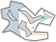
Figure 10: A 1-separator (blue), a 2-separator (orange), and a 3-separator (green).

Theorem 4.2.

Let $S$ be a set of $n$ point sites in a polygonal domain $P$ with $m$ vertices. A balanced sp-separator exists and it can be computed in $O(n^{2}\log m+nm\log m)$ time.

We first give a constructive proof for the existence of a balanced sp-separator, using a similar approach to Abam et al. [3]. Then, we fill in some algorithmic details and prove that the algorithm runs in $O(n^{2}\log m+nm\log m)$ time.

Existence of a separator.

We start by trying to find a 1-separator from an arbitrary fixed point $u\in\partial P$ to a point $v\in\partial P$. The point $v$ is moved clockwise along the boundary of $P$, starting at $u$, to find a separator satisfying our constraints, i.e. $P_{\ell}$ contains between $2n/9$ and $2n/3$ sites of $S$. This way, we either find a balanced 1-separator, or jump over at least $2n/3-2n/9=4n/9$ sites at a point $v$. In this case, the region bounded by two shortest paths between $u$ and $v$ contains at least $4n/9$ sites. We then try to find a 2- or 3-separator contained within this region.

To find a 2- or 3-separator, we construct a sequence of 3-separators $\Delta_{0}\supset\Delta_{1}\supset...\supset\Delta_{k}$, where either the final 3-separator $\Delta_{k}$ contains between $2n/9$ and $2n/3$ sites, or we find a balanced 2-separator within $\Delta_{k}$. During the construction, the invariant that $|\Delta_{i}\cap S|\geq 2n/9$ is maintained. The first 3-separator, $\Delta_{0}$, has as corners the two points $u$ and $v$ on $\partial P$ from before, and a point $w$, which is an arbitrary point on one of the two shortest paths connecting $u$ and $v$. So, $\Delta_{0}$ is exactly the region bounded by the two shortest path connecting $u$ and $v$ that contains at least $4n/9$ sites.

Whenever $\Delta_{i}$ contains at most $2n/3$ sites, we are done. If not, we find $\Delta_{i+1}$ as follows. If $\Delta_{i}$ is a degenerate 3-separator, we simply select a subpath of the shortest path that contains $2n/3$ sites. Similarly, if at least $2n/9$ sites lie on any of the bounding shortest paths. If neither of these cases holds, then there are at least $2n/3+1-3(2n/9-1)=4$ sites in the interior of $\Delta_{i}$. In the following, we find a 3-separator $\Delta_{i+1}$ with either $|\Delta_{i+1}\cap S|<|\Delta_{i}\cap S|$, or $|\text{Int}(\Delta_{i+1})\cap S|<|\text{Int}(\Delta_{i})\cap S|$, or a valid 2-separator contained within $\Delta_{i}$. Because each $\Delta_{i}$ contains either fewer sites, or fewer sites in its interior, than its predecessor, we eventually find a 3-separator with the desired number of sites, or we end up in one of the easy degenerate cases. In the following description, we drop the subscript $i$ for ease of description.

We define a good path to be a path from a point $p\in\Delta$ to a corner $u$ to be a shortest path $\pi(p,u)$ that is fully contained within $\Delta$. To make sure our definition is also correct when one of the corners lies inside $\Delta$, we do not allow the path to cross $\pi(v,w)$. See Figure 11 for an illustration. Essentially, we see the coinciding part of the shortest paths as having an infinitesimally small separation between them. The following provides a formal definition of a good path.

Definition 4.3.

A shortest path $\pi(p,u)$ from a point $p$ that lies in a 3-separator $\Delta$ to a corner $u$ of $\Delta$, is a good path if it is fully contained within $\Delta$, and $\pi(p,u)$ is a shortest path in the polygonal domain $P\cap\Delta$, where the outer polygon is $\Delta$.

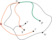
Figure 11: Of the shortest paths $\pi(p,u)$, $\pi(q,u)$, and $\pi(r,u)$ only $\pi(p,u)$ is a good path.

We consider the closed region $Z_{u}\subset\Delta$ such that for every $p\in Z_{u}$ there is a good path to $u$. Because for any $p^{\prime}$ on a good path $\pi(p,u)$ the path $\pi(p^{\prime},u)$ is also a good path, $Z_{u}$ is connected. $Z_{u}$ is bounded by $\pi(u,v)$, $\pi(u,w)$, $\partial H$, and a curve $B_{u}$ that connects $v$ to $w$, see Figure 12. Because we do not consider $\partial H$ to be part of $B_{u}$, this is a possibly disconnected curve that consists of edges from the shortest path map of $u$ and $\Delta$. The shortest path map of a point $p$ in a polygonal domain $P$ partitions the free space into maximal regions, such that for any two points in the same region the shortest paths from $u$ to both points use the same vertices of $P$ [37]. We call the curves of the shortest path map for which there are two topologically distinct paths from $p$ to any point on the curve walls. We prove the following lemma of Abam et al. [3] for our definition of a good path.

Lemma 4.4 (Lemma 3.2 of [3]).

For any point $z\in B_{u}$, there are good paths $\pi(z,u)$, $\pi(z,v)$, and $\pi(z,w)$ to the three corners of $\Delta$.

Proof 4.5.

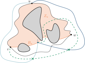
Figure 12: Any path from $z$ to $v$ that exits $\Delta$ through $\pi(u,w)$ must intersect a path from $z$ to $u$.

By definition of $B_{u}$, there is a good path from $z$ to $u$. When $z$ lies on $\pi(v,w)$, the subpaths of $\pi(v,w)$ from $z$ to $v$ and to $w$ are good paths. So, assume $z\notin\pi(v,w)$. We will prove by contradiction that there is a good path from $z$ to $v$, and by symmetry from $z$ to $w$. Suppose there is no good path from $z$ to $v$. Because $z$ is on $B_{u}$, there is also a shortest path from $z$ to $u$ that is not a good path, so it is not contained within $\Delta$, or it crosses $\Delta$. This path $\pi(z,u)$ must exit (or cross) $\Delta$ through $\pi(v,w)$, because otherwise the path could simply continue along $\pi(v,u)$ or $\pi(w,u)$ and stay within $\Delta$. Similarly, $\pi(z,v)$ must exit $\Delta$ through $\pi(u,w)$. The path $\pi(z,u)$ either goes around $v$ or $w$, as shown in Figure 12. In both cases, any path to $v$ that starts at $z$ and exits (or crosses) through $\pi(u,w)$ and does not intersect $\pi(u,w)$ again, must intersect the path $\pi(z,u)$. As these shortest paths start at the same point, this is a contradiction with the fact that two shortest paths can only cross once.

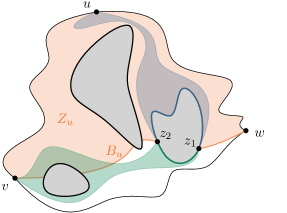
Figure 13: The region $Z_{u}$ where all points have good paths to $u$. In blue and green the 2-separator with corners $z_{1},u,z_{2}$ and $z_{1},v,z_{2}$, respectively.

This lemma implies that for any point $z$ on $B_{u}$, the 3-separator with corners $u$, $v$, and $z$ is contained within $\Delta$. We use this observation by moving a point $z$ along $B_{u}$ from $w$ to $v$. At the start, the 3-separator defined by $u$, $v$, and $z$, which we denote by $T_{z}$, is equal to $\Delta$. At the end, $T_{z}$ is equal to the degenerate 3-separator $\pi(u,v)$. Note that, in contrast to the situation of Abam et al. [3] for a terrain, $B_{u}$ is not necessarily continuous, as it can be interrupted by holes. But, if $B_{u}$ intersects a hole, it intersects this hole exactly twice, because $Z_{u}$ is connected. A directed walk along $B_{u}$, jumping at holes, is thus still well-defined. We walk a point $z$ along $B_{u}$ until one of the following happens: (1) $|S\cap T_{z}|$ or $|S\cap\text{Int}(T_{z})|$ decreases, or (2) $z$ encounters a hole.

In case (1), either $T_{z}$ contains at least $2n/9$ sites, then we set $\Delta_{i+1}:=T_{z}$, or we jump over at least $2n/3-2n/9=4n/9$ sites. This can happen because the shortest path to $u$, to $v$, or both jump over a hole. We assume the path to $u$ jumps, the approach for when the path to $v$ jumps is symmetric. The 3-separator $u,z,w^{\prime}$, with $w^{\prime}$ on one of the two $\pi(z,u)$, could contain the same number of sites, in the closure and in its interior, as $\Delta$. Therefore, we select an arbitrary site $s\in S$ that lies in the region bounded by the two shortest paths. We then consider the two 3-separators with $u$, $z$, and $s$ as corners. As $s$ now lies on the boundary of the 3-separators, both of these separators contain less sites in their interior than $\Delta$. And, as they partition a region that contains at least $4n/9$ sites, one of them contains at least $2n/9$ sites. We set $\Delta_{i+1}$ to be this 3-separator.

In case (2), let $z_{1}$ denote the point we encounter the hole $H_{i}$, and $z_{2}$ be the point where $B_{u}$ exits $H_{i}$, see Figure 13. Whenever $|T_{z_{2}}\cap S|\geq 2n/9$, we simply continue the walk at $z_{2}$, until we again end up in one of the two cases. If not, then there are at least $2n/3-2n/9=4n/9$ sites in $T_{z_{1}}\setminus T_{z_{2}}$, because $T_{z_{2}}\subset T_{z_{1}}$. Note that $T_{z_{1}}\setminus T_{z_{2}}$ is exactly the union of the two 2-separators $z_{1},u,z_{2}$ and $z_{1},v,z_{2}$. This means that either the 2-separator $z_{1},u,z_{2}$ or $z_{1},v,z_{2}$ contains at least $2n/9$ sites. Suppose that the separator including $u$ contains at least $2n/9$ sites. We then try to find a balanced 2-separator $z_{1},u,z^{*}$ with $z^{*}\in\partial H_{i}$ that is contained within the 2-separator $z_{1},v,z_{2}$. For each point $z^{*}\in\partial H_{i}$ on the “$u$-side” of $H_{i}$ (blue in Figure 13), $\pi(z^{*},u)$ is contained within the 2-separator $z_{1},u,z_{2}$, as it cannot cross $\pi(z_{1},u)$ and $\pi(z_{2},u)$. As we did to find a 1-separator, we walk $z^{*}$ along $\partial H_{i}$ from $z_{1}$ to $z_{2}$ on the “$u$-side”. As before, we now find a balanced 2-separator, and we are done, or we jump over at least $2n/3-2n/9=4n/9$ sites. Again, this region does not necessarily contain less sites than $\Delta$, thus we continue as before by selecting a site $s$ in this region as the third corner of $\Delta_{i+1}$. Similarly, when the 2-separator with $v$ as a corner contains more than $2n/9$ sites, we walk $z^{*}$ along the other side of $H_{i}$ and consider the 2-separator $z_{1},v,z^{*}$.

Running time.

Next, we discuss the details and running times of the general algorithm that computes a balanced sp-separator. We choose for $u$ the vertex of $\partial P$ with smallest $y$-coordinate. We first construct the augmented shortest path map $\mathit{SPM}_{u}$ of $u$. In the augmented shortest path map, we include the shortest path tree of $u$, essentially triangulating each region in the shortest path map using the vertices of $P$. This can be constructed in $O(m\log m)$ time [37] (or even $O(m+h\log h)$ time, where $h$ is the number of holes in $P$). We then find the region of $\mathit{SPM}_{u}$ that contains $p\in S$ for all $p$ in $O(n\log m)$ time. We call the vertices of $\partial P$ and $SPM_{u}\cap\partial P$ breakpoints, see Figure 14. After sorting these breakpoints along the boundary of $P$, we can easily move $v$ along the boundary from one breakpoint to the next, while keeping track of the number of sites in $P_{\ell}$. When moving $v$ from one breakpoint to the next, there is only one new triangle included in $P_{\ell}$. Whenever we encounter a wall breakpoint $b$, we additionally check the number of sites that lie between the two shortest paths $\pi(u,b)$. If this number is too large, we continue to find a 2-, or 3-separator in the region bounded by these shortest paths. If not, then we either find a suitable 1-separator at one of the breakpoints, or, if the difference in $|S_{\ell}|$ between two consecutive breakpoints $v^{\prime}$ and $v$ is too large, we find a 1-separator with corners $u$ and a point $v^{*}$ between the two breakpoints. As only sites in the triangle $vv^{\prime}w$ are of interest, where $w$ is the predecessor of $v$ in $\pi(u,v)$, this point can easily be found. When too many sites lie on a line through $w$ in this final triangle, we select a subpath of this line that contains the desired number of sites as our (degenerate) separator. There are $O(m)$ breakpoints, thus in $O((m+n)\log m)$ time we either find a balanced 1-separator, or we find a region bounded by two shortest paths where we will find a 2- or 3-separator.

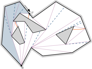
Figure 14: The augmented shortest path map of $u$. The walls of $\mathit{SPM}_{u}$ are the orange edges. For $v$ in its current position $P_{\ell}$ is given by the blue region.

We then construct the sequence of $O(n)$ 3-separators $\Delta_{0}\supset\Delta_{1}\supset...\supset\Delta_{k}$. To go from a 3-separator $\Delta_{i}$ with corners $u,v,w$ to the next 3-separator $\Delta_{i+1}$, we need to construct the curve $B_{u}$. As stated before, this (possibly disconnected) curve consists of edges from the shortest path map of $u$. We thus construct the augmented shortest path map $\mathit{SPM}_{u}$ in $O(m+h\log h)$ time. Then we find $B_{u}$ by labelling the shortest path map regions in $\Delta$ whose shortest path is contained in $\Delta$, and selecting all edges that are between a labelled and a non-labelled region. After performing a point location in the shortest path map for each site in $S$, we can walk $z$ along $B_{u}$ while keeping track of $|S\cap T_{z}|$ as we did along the polygon boundary. When we encounter a hole, we first check whether the 2-separator with $u$ or $v$ contains more sites, for example by explicitly constructing these 2-separators and point locating the sites, and then continue along the boundary of the hole on the $u$- or $v$-side. During the procedure to find $\Delta_{i+1}$, we perform a constant number of point locations per site, thus the running time is $O((n+m)\log m)$. As we lose at least one site in each iteration, the sequence has maximum length $n$, and the total running time is $O(n^{2}\log m+nm\log m)$.

Correction of a technical issue in Abam et al. [3].

Abam et al. [3] present an approach to find a balanced sp-separator on a terrain $\mathcal{T}$. They define an sp-separator as either a 1-separator or a 3-separator, where the three shortest paths are disjoint except for their mutual endpoints. However, on a polyhedral terrain these paths might also not be disjoint. This can, for example, happen when choosing a site $s$ in the area bounded by two shortest paths as a new corner, see Figure 15. Their subsequent definition of a good path, which is simply a shortest path contained within $\Delta$, would then imply that the entire interior of the box, including the blue region in Figure 15(a), is contained in $Z_{u}$. The question is then how we move $z$ from $w$ to $v$. If we would move $z$ along $\pi(w,v)$ at the start, the site $w$ will immediately enter the interior of the 3-separator $u,v,z$, see Figure 15(b). The number of sites in the interior has thus actually increased instead of decreased. In a polyhedral terrain, we can define a good path similar to Definition 4.3, but then consider the path $\pi(p,u)$ in the polyhedral terrain $\mathcal{T}\cap\Delta$. Using our renewed definition, the proof of Abam et al. [3] also holds in the case of coinciding edges on a terrain.

(a) The region $Z_{u}$ according to our definition of a good path in orange. The region $Z_{u}$ according to [3] includes the blue region.

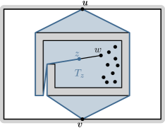
(b) The 3-separator $T_{z}$ has more sites in its interior than the original 3-separator $\Delta$.

Figure 15: A polygonal domain where the shortest paths in the separator $\Delta$ with corners $u,v,w$ are not disjoint.

5 Spanners in a polygonal domain

We consider a set of point sites $S$ that lie in a polygonal domain $P$ with $m$ vertices and $h$ holes. Let $\partial P$ denote the boundary of the outer polygon. In Section 5.1, we first discuss how to obtain a simple geodesic spanner for a polygonal domain, using the separator of Section 4. As before, the complexity of this spanner can be high. In Section 5.2.1, we discuss an adaptation to the spanner construction that achieves lower-complexity spanners, where the edges in the spanner are no longer shortest paths.

5.1 A simple geodesic spanner

A straightforward approach to construct a geodesic spanner for a polygonal domain would be to use the same construction we used for a simple polygon in Section 3.1. As discussed in Section 4, we cannot split the polygon into two subpolygons by a line segment $\lambda$. However, to apply our 1-dimensional spanner, we require only that the splitting curve $\lambda$ is a shortest path in $P$. Instead of a line segment, we use the balanced sp-separator of Section 4 to split the polygonal domain. There are three types of such a separator: a shortest path between two points on $\partial P$ (1-separator), two shortest paths starting at the same point and ending at the boundary of a single hole (2-separator), three shortest paths $\pi(u,v)$, $\pi(v,w)$, and $\pi(u,w)$ with $u,v,w\in P$ (3-separator). See Figure 10 for an illustration and Definition 4.1 for a formal definition. Let $P_{\ell}$ be the polygonal domain to the left of $\lambda$, when $\lambda$ is a 1-separator, and interior to $\lambda$, when $\lambda$ is a 2- or 3-separator. Symmetrically, $P_{r}$ is the domain to the right of $\lambda$ for a 1-separator and exterior to $\lambda$ for a 2-, or 3-separator. As before, let $S_{\ell}$ be the sites in the closed region $P_{\ell}$, and $S_{r}:=S\setminus S_{\ell}$. To compute a spanner on the set $S$, we project the sites to each of the shortest paths defining the separator, and consecutively run the 1-dimensional spanner algorithm once on each shortest path. Note that these projections are no longer unique, as there might be two topologically distinct shortest paths to $\lambda$, but we can simply select an arbitrary one to obtain the desired spanning ratio and spanner complexity. We then add the edge $(p,q)$ to our spanner $\mathcal{G}$ for each edge $(p_{\lambda},q_{\lambda})$ in the 1-dimensional spanners. Finally, we recursively compute spanners for the sites $S_{\ell}$ in $P_{\ell}$ and $S_{r}$ in $P_{r}$, just like in the simple polygon case.

Whenever the sp-separator intersects a single hole at two or more different intervals, then part of $P_{\ell}$ or $P_{r}$ becomes disconnected. When this happens, we simply consider each connected polygonal domain as a separate subproblem, and recurse on all of them. Let $n_{i}$ and $m_{i}$ denote the number of sites and worst-case complexity of a shortest path in subproblem $i$. This means that only reflex vertices are counted for $m_{i}$, which are the only relevant vertices for the spanner complexity. The sites are partitioned over the subproblems, so we have $\sum_{i}n_{i}=n$. The only new vertices (not of $P$) that can be included in the subproblems are the at most three corners of the separator. Each vertex can be a reflex vertex in only one of the subproblems, thus $\sum_{i}m_{i}\leq m+3$. In the recursion, an increase in the number of subproblems means that we might have more than $c\cdot 2^{i}$ vertices not of $P$ at level $i$, but the depth of the recursion tree is then proportionally decreased. All further proofs on complexity of our spanners are written in term of $P_{\ell}$ and $P_{r}$, but translate to the case of multiple subproblems.

Next, we analyze the spanner construction using any 1-dimensional additively weighted $t$-spanner of size $O(n\log n)$.

Lemma 5.1.

The graph $\mathcal{G}$ is a geodesic $3t$-spanner of size $O(n\log^{2}n)$.

Proof 5.2.

As the 1-dimensional spanner has size $O(n\log n)$, there are still $O(n\log^{2}n)$ edges in $\mathcal{G}$. What remains is to argue that $\mathcal{G}$ is a $3t$-spanner. Let $p,q$ be two sites in $S$. In contrast to the simple polygon case, a shortest path between two sites $p,q$ in $S_{\ell}$ (resp. $S_{r}$) is not necessarily contained in $P_{\ell}$ (resp. $P_{r}$). Therefore, we distinguish two different cases: either $\pi(p,q)$ is fully contained within $P_{r}$ or $P_{\ell}$, or there is a point $r\in\pi(p,q)\cap\lambda$ for some shortest path $\lambda$ of the separator. In the first case, there exists a path in $\mathcal{G}$ of length at most $3td(p,q)$ by induction. In the second case, we have

$$d_{\mathcal{G}}(p,q)\leq d_{\mathcal{G}_{\lambda}}(p,q)\leq td_{w}(p_{\lambda},q_{\lambda})=t(d(p,p_{\lambda})+d(p_{\lambda},q_{\lambda})+d(q,q_{\lambda})).$$ (4)

Additionally, we use that $d(p_{\lambda},q_{\lambda})\leq d(p_{\lambda},r)+d(r,q_{\lambda})$ and $d(p_{\lambda},r)\leq d(p_{\lambda},p)+d(p,r)$, because of the triangle inequality, so

$$d(p_{\lambda},q_{\lambda})\leq d(p_{\lambda},r)+d(q_{\lambda},r)\leq d(p_{\lambda},p)+d(p,r)+d(q_{\lambda},q)+d(q,r)\leq 2d(p,q).$$

It follows that $d_{\mathcal{G}}(p,q)\leq 3td(p,q)$.

Applying the simple 1-dimensional spanner of Section 2 results in a 6-spanner. However, using the refinement of Lemma 3.3, we again obtain a $(2+\varepsilon)$-spanner.

5.2 Low complexity spanners in a polygonal domain

To obtain spanners of low complexity in a simple polygon, we formed groups of sites, such that shortest paths within a group were disjoint from shortest paths of other groups. We proposed two different ways of forming these groups, based on the shortest path tree of the central site $c$, and based on the shorest path tree of the separator $\lambda$. Both of these approaches do not directly lead to a low complexity spanner in a polygonal domain, as we explain next.

Both methods can still be applied in a polygonal domain, as the shortest path tree of both a site and a shortest path is still well-defined. However, it does not give us the property that we want for our groups. In particular, the second property discussed in Lemma 3.24: each vertex of $P$ is only used by shortest paths within $O(1)$ groups, does not hold. This is because the shortest path between two vertices $u,v$ is not necessarily homotopic to the path $\pi(u,c)\cup\pi(c,v)$. Thus paths within a group can go around a certain hole, while their shortest paths to $c$ (or $\lambda$) do not. See Figure 16 for an example. The construction can easily be expanded to ensure there are more sites in each group, by simply adding as many sites very close to the existing ones, or to more than three groups, by adding an additional hole above the construction with two corresponding sites. Consequently, the property that each vertex of $P$ is used only by shortest paths within $O(1)$ groups does not hold.

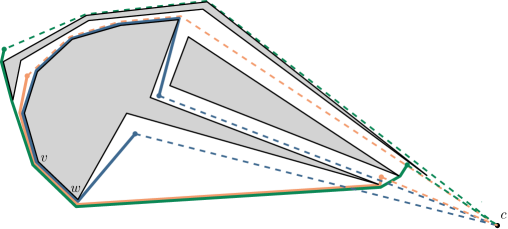
Figure 16: Assigning the sites to groups based on the shortest path tree of $c$, as described in Section 3.2.1, forms these colored groups. The shortest path from each site to $c$ is shown dashed. Each shortest path between two sites of a group contains both vertices $v$ and $w$.

So far, we assumed that every edge $(p,q)\in E$ is a shortest path between $p$ and $q$. To obtain a spanner of low complexity, we can also allow an edge between $p$ and $q$ to be any path between the two sites. Note that our lower bounds still hold in this case. In the lower bound for a $(3-\varepsilon)$-spanner (Figure 4), every path between $p\in S_{\ell}$ and $q\in S_{r}$ has complexity $\Theta(m)$, and in the general lower bound (Figure 18) we can easily adapt the top side of the polygon such that any path between two sites $p,q$ has the same complexity as $\pi(p,q)$.

5.2.1 A $12$-spanner of complexity $O(m\sqrt{n}+n\log^{2}n)$

To obtain a low complexity spanner in a polygonal domain, we adapt our techniques for the simple-polygon $4\sqrt{2}$-spanner in such a way that we avoid the problems we just sketched. The main difference with the simply polygon approach is that for an edge $(p_{\lambda},q_{\lambda})$ in the 1-dimensional spanner, the edge $(p,q)$ that we add to $\mathcal{G}$ is no longer $\pi(p,q)$. Instead, let $(p,q)$ be the shortest path from $p$ to $q$ via $p_{\lambda}$ and $q_{\lambda}$, excluding any overlap of the path. We denote this path by $\pi_{\lambda}(p,q)$. This path is not unique, for example when $\pi(p,p_{\lambda})$ is not unique, but again choosing any such path will do. Formally, $\pi_{\lambda}(p,q)$ is defined as follows.

Definition 5.3.

The path $\pi_{\lambda}(p,q)$ is given by:

• $\pi(p,p_{\lambda})\cup\pi(p_{\lambda},q_{\lambda})\cup\pi(q_{\lambda},q)$, where $\pi(p_{\lambda},q_{\lambda})\subseteq\lambda$, if $\pi(p,p_{\lambda})$ and $\pi(q,q_{\lambda})$ are disjoint,

• $\pi(p,r)\cup\pi(r,q)$, where $r$ denotes the closest point to $p$ of $\pi(p,p_{\lambda})\cap\pi(q,q_{\lambda})$, otherwise.

One of the properties that we require of the groups, see Lemma 3.8, has changed, namely that each vertex of $P$ is only used by shortest paths within $O(1)$ groups. Instead of the shortest paths between sites in a group, we consider the paths $\pi_{\lambda}(p,q)$ of Definition 5.3. The following lemma shows that we can obtain a spanner with similar complexity as in a simple polygon when groups adhere to this adjusted property.

Lemma 5.4.

If the groups adhere to the following properties, then $\mathcal{G}$ has complexity $O(m\sqrt{n}+n\log^{2}n)$:

1. each group contains $\Theta(\sqrt{n})$ sites, and

2. each vertex of $P$ is used by paths $\pi_{\lambda}$ within $O(1)$ groups.

Proof 5.5.

Note that the complexity of any path $\pi_{\lambda}(p,q)$ is $O(m)$, as it can use a vertex of $P$ at most once. Thus the proof of Lemma 3.8 directly implies that the complexity of the edges in one level of the 1-dimensional spanner is $O(m\sqrt{n}+n)$.

In the 1-dimensional recursion, splitting the sites by $O$ no longer corresponds to a horizontal split in the polygon. However, the paths $\pi(p,p_{\lambda})$, $p\in S_{\ell}$, are still disjoint from the paths $\pi(q,q_{\lambda})$, $q\in S_{r}$. For the two subproblems generated by the split by $O$ it thus still holds that $m_{1}+m_{2}=m$, where $m_{i}$ denotes the maximum complexity of a path in subproblem $i$. Lemma 3.6 states that this recursion solves to $O(m\sqrt{n}+n\log n)$.

In the recursion where the domain is partitioned into two subpolygons $P_{\ell}$ and $P_{r}$, we now add at most three new vertices to the polygonal domain, namely the three corners of the sp-separator. Each vertex of $P$ can only be a reflex vertex in either $P_{\ell}$ or $P_{r}$, so $m_{1}+m_{2}\leq m+3$. Lemma 3.6 implies that this recursion for the complexity solves to $O(m\sqrt{n}+n\log^{2}n)$.

As in Lemma 3.24, we form the groups based on the traversal of the shortest path tree $\mathit{SPT}_{\lambda}$. We again include all sites in $S$ in the shortest path tree. Whenever a node $v$ of $\lambda$ has multiple children, we let all nodes that correspond to vertices/sites that lie to the left of $\lambda$ come before nodes that correspond to vertices/sites that lie to the right of $\lambda$ in the in-order traversal. Within these sets, the vertices/sites are ordered from bottom to top, as seen from $v$. See Figure 17 for an example. The subtree rooted at the start and end point of $\lambda$ is simply a part of the shortest path tree of the start/end point. The first $\lceil\sqrt{n}\rceil$ sites in the in-order traversal are in $S_{1}$, the second $\lceil\sqrt{n}\rceil$ in $S_{2}$, etc.

Figure 17: The shortest path tree $\mathit{SPT}_{\lambda}$ and the corresponding group assignment.

Clearly, these groups adhere to property 1 of Lemma 5.4. To show these groups adhere to property 2, we again consider for each group $S_{i}$ the minimal subtree $\mathcal{T}_{i}$ of $\mathit{SPT}_{\lambda}$ that contains all $p\in S_{i}$. Whenever there is more than one vertex of $\lambda$ in $\mathcal{T}_{i}$, we choose the leftmost of these vertices as the root of $\mathcal{T}_{i}$.

Lemma 5.6.

An edge $\pi_{\lambda}(p,q)$ with $p_{\lambda},q_{\lambda}\in S_{i}$ bends only at vertices in $\mathcal{T}_{i}$.

Proof 5.7.

The path $\pi_{\lambda}(p,q)$ is a subpath of $\pi(p,p_{\lambda})\cap\pi(p_{\lambda},q_{\lambda})\cap\pi(q,q_{\lambda})$. In particular, it is the path from $p$ to $q$ in $\mathcal{T}_{i}$ via their lowest common ancestor. This is $p_{\lambda}$ or $q_{\lambda}$ when $\pi(p,p_{\lambda})\cap\pi(q,q_{\lambda})=\emptyset$ and the vertex $r$, as in Definition 5.3, otherwise.

Lemma 5.8.

Any vertex in $\mathit{SPT}_{\lambda}$ occurs in at most two trees $\mathcal{T}_{i}$ and $\mathcal{T}_{j}$ as a non-root node.

Proof 5.9.

Follows directly from the proof of Lemma 3.14.

Except for the root nodes, property 2 thus holds. As each $\mathcal{T}_{i}$ has only one root node by definition, the number of groups using a single root node $v$ in their paths may be large, but the sum of the number of groups that use a node over all root nodes is still $O(\sqrt{n})$. From this and Lemma 5.4 we conclude that $\mathcal{G}$ has complexity $O(m\sqrt{n}+n\log^{2}n)$.

Lemma 5.10.

The graph $\mathcal{G}$ is a geodesic $12$-spanner of size $O(n\log^{2}n)$.

Proof 5.11.

The number of edges is exactly the same as in the $4\sqrt{2}$-spanner in a simple polygon. The way the groups are formed in the construction of the 1-dimensional spanner $\mathcal{G}_{\lambda}$ does not influence its spanning ratio, thus $\mathcal{G}_{\lambda}$ is a 4-spanner (see Lemma 3.16). Note that even for our redefined edges in $\mathcal{G}$ it holds that $d_{\mathcal{G}}(p,q)\leq d_{\mathcal{G}_{\lambda}}(p_{\lambda},q_{\lambda})$. Lemma 5.1 then directly implies that $\mathcal{G}$ is a 12-spanner.

5.2.2 A $(2k+\varepsilon)$-spanner of complexity $O(mn^{1/k}+n\log^{2}n)$

The generalization of the construction, discussed in Section 3.2.2, where $\Theta(n^{1/k})$ groups are recursively partitioned into smaller groups, is also applicable in a polygonal domain. As our groups adhere to the required properties, the complexity of this spanner remains $O(mn^{1/k}+n\log^{2}n)$, as in the simple polygon, but the spanning ratio increases to $6k$. We can also apply the refinement discussed in Lemma 3.3 in the construction of the (at most three) 1-dimensional spanners. This improves the spanning ratio to $2k+\varepsilon$ while increasing the complexity by only a constant factor depending only on $\varepsilon$ and $k$.

Lemma 5.12.

Let $S$ be a set of $n$ point sites in a polygonal domain $P$ with $m$ vertices, and let $k\geq 1$ be any integer constant. For any constant $\varepsilon>0$, there exists a geodesic $(2k+\varepsilon)$-spanner of size $O(c_{\varepsilon,k}n\log^{2}n)$ and complexity $O(c_{\varepsilon,k}(mn^{1/k}+n\log^{2}n))$, where $c_{\varepsilon,k}$ is a constant depending only on $\varepsilon$ and $k$.

5.3 Construction algorithm

In this section we discuss an algorithm to compute the geodesic spanners of Section 5.2. The following gives an overview of the algorithm that computes a $6k$-spanner of complexity $O(mn^{1/k}+n\log^{2}n)$ in $O(n^{2}\log m+nm\log m)$ time.

1. Find an sp-separator such that $P$ is partitioned into two polygons $P_{\ell}$ and $P_{r}$, and $S_{\ell}$ contains at least $2n/9$ and at most $2n/3$ sites using the algorithm of Theorem 4.2.

2. For each shortest path $\lambda$ of the separator:

   1. For each $p\in S$ find the weighted point $p_{\lambda}$ on $\lambda$ and add this point to $S_{\lambda}$ using the algorithm of Lemma 5.13.

   2. Compute an additively weighted 1-dimensional spanner $\mathcal{G}_{\lambda}$ on the set $S_{\lambda}$.

   3. For every edge $(p_{\lambda},q_{\lambda})\in E_{\lambda}$ add the edge $(p,q)=\pi_{\lambda}(p,q)$ to $\mathcal{G}$.

3. Recursively compute spanners for $S_{\ell}$ in $P_{\ell}$ and $S_{r}$ in $P_{r}$.

The algorithm start by finding a balanced sp-separator. According to Theorem 4.2 this takes $O(n^{2}\log m+nm\log m)$ time. We then continue by building a 1-dimensional additively weighted spanner on each of the shortest paths defining $\lambda$ as follows.

Lemma 5.13.

We can compute the closest point $p_{\lambda}$ on $\lambda$ and $d(p,p_{\lambda})$ for all sites $p\in S$, and the shortest path tree $\mathit{SPT}_{\lambda}$, in $O((m+n)\log m)$ time.

Proof 5.14.

Hershberger and Suri [27] show how to build the shortest path map of a point site in a polygonal domain in $O(m\log m)$ time. They also note that this extends to non-point sources, such as line segments, and to $O(m)$ sources, without increasing the running time. We can thus build the shortest path map of $\lambda$ in $P$ in $O(m\log m)$ time, using that $\lambda$ has complexity $O(m)$. After essentially triangulating each region of the shortest path map using the vertices of $P$, we obtain $\mathit{SPT}_{\lambda}$ in the same time bound. After building a point location data structure for this augmented shortest path map, we can query it for each site $p\in S$ to find $p_{\lambda}$ and $d(p,p_{\lambda})$ in $O(\log m)$ time.

Lemma 5.15.

Given $\mathit{SPT}_{\lambda}$, we can construct a $4$-spanner $\mathcal{G}_{\lambda}$ on the additively weighted points $S_{\lambda}$, where the groups adhere to the properties of Lemma 5.4, in $O(n\log n+m)$ time.

Proof 5.16.

As in Lemma 3.24, we can reuse $\mathit{SPT}_{\lambda}$ to form the groups based on the ordering produced by an in-order traversal of the tree. See Section 5.2.1 for an exact description of this ordering. The ordering allows us to form the groups for a level of the 1-dimensional spanner in $O(n)$ time, thus the total running time is $O(n\log n)$.

For the general $2k$-spanner for additively weighted sites, using the ordering of the sites and Lemma 3.26 to build the tree of groups bottom up implies that we can construct this spanner in $O(n\log n+m)$ time as well.

After computing the additively weighted spanner $\mathcal{G}_{\lambda}$, we add edge $(p,q)=\pi_{\lambda}(p,q)$ to $\mathcal{G}$ for every edge $(p_{\lambda},q_{\lambda})\in\mathcal{G}_{\lambda}$. We can either compute and store these edges explicitly, which would take time and space equal to the complexity of all added edges, or we can store them implicitly by only storing the points $p_{\lambda}$ and $q_{\lambda}$, or the point $r$ from Definition 5.3 when the paths are not disjoint. The point $r$ is the lowest common ancestor of the nodes $p$ and $q$ in $\mathit{SPT}_{\lambda}$. This can be computed in $O(1)$ time after $O((n+m)\log(n+m))$ preprocessing time [5].

As there are at most three shortest path that define the separator, step 2 takes $O((n+m)\log(n+m))$ time in total. This means that the time used to construct the balanced sp-separator is the dominant term. Because this step even takes quadratic time, it also dominates in the recursion. After applying the refinement of Lemma 3.3, we obtain the following theorem.

Theorem 5.17.

Let $S$ be a set of $n$ point sites in a polygonal domain $P$ with $m$ vertices, and let $k\geq 1$ be any integer constant. For any constant $\varepsilon>0$, we can build a geodesic $(2k+\varepsilon)$-spanner of size $O(c_{\varepsilon,k}n\log^{2}n)$ and complexity $O(c_{\varepsilon,k}(mn^{1/k}+n\log^{2}n))$ in $O(n^{2}\log m+nm\log m+K)$ time, where $c_{\varepsilon,k}$ is a constant depending only on $\varepsilon$ and $k$, and $K$ is the output complexity.

5.4 A $(2k+\varepsilon)$-spanner with a dependence on $\sqrt{h}$

Let $h$ denote the number of holes in the polygonal domain $P$. In this section, we describe an alternative approach to Section 5.2 to compute a $(2k+\varepsilon)$-spanner of low complexity. Here, we do not use the balanced shortest-path separator of Section 4, which greatly reduces the running time, at the cost of making both the size and complexity of the spanner dependent on $\sqrt{h}$.

Abam et al. [1] describe how to decompose a polygonal domain with $h$ holes into $O(h)$ simple polygons using $O(h)$ vertical segments called splitting segments. Furthermore, each each simple polygon has at most three splitting segments on its boundary. Instead of partitioning the polygonal domain by a shortest path, they then apply a graph separator theorem to partition the simple polygons into three sets $A,B,C$ such that $|C|=O(\sqrt{h})$, any path from a site $p\in A$ to $q\in B$ intersects $C$, and $|S_{A}|,|S_{B}|\leq 2|S|/3$, where $S_{A}$ (resp. $S_{B}$) denotes the set of sites that lie in a polygon in $A$ (resp. $B$). We can compute a spanner for the entire polygonal domain by building our 1-dimensional spanner on each of the $O(\sqrt{h})$ splitting segments, building the simple polygon spanner for each of the $O(\sqrt{h})$ simple polygons in $C$ and recursively computing spanners for $A$ and $B$.

Next, we analyze the spanning ratio, size, and complexity of $\mathcal{G}$ when using the simple-polygon spanner of Theorem 3.28 and the corresponding 1-dimensional spanner for the spanners on the splitting segments. The spanning ratio of the spanner remains $2k+\varepsilon$, because a shortest path between two sites $p,q$ either crosses a splitting segment, whose spanner then bounds $d_{\mathcal{G}}(p,q)$, or stays within a simple polygon, in which case the simple polygon spanner bounds $d_{\mathcal{G}}(p,q)$.

In a single level of the recursion, the spanners on the splitting segments contribute $O(c_{\varepsilon,k}\sqrt{h}n\log n)$ edges, thus the spanners on all of the splitting segments contribute $O(c_{\varepsilon,k}\sqrt{h}n\log^{2}n)$ edges in total. For each simple polygon, we build the spanner of Theorem 3.28, which has $O(c_{\varepsilon,k}n_{i}\log^{2}n_{i})$ edges, where $n_{i}$ denotes the number of sites in simple polygon $i$. Because $\sum_{i}n_{i}=n$, these contribute $O(c_{\varepsilon,k}n\log^{2}n)$ edges in total. The number of edges is thus $O(c_{\varepsilon,k}\sqrt{h}n\log^{2}n)$.

The spanner complexity over all 1-dimensional spanners built on the splitting segments is $O(c_{\varepsilon,k}\sqrt{h}(mn^{1/k}+n\log^{2}n))$. Similarly as for the number of edges, the complexity over all simple-polygon spanners is only $O(c_{\varepsilon,k}(mn^{1/k}+n\log^{2}n))$.

The number of edges and the complexity of the spanner has thus increased by a factor $\sqrt{h}$ with respect to the spanner of Theorem 5.17, but building the spanner is significantly easier, as we do not need a balanced sp-separator here. After computing the vertical decomposition of $P$ in $O(m\log m)$ time, we select the segments that have at least one of their endpoints on the rightmost or leftmost vertex of a hole as splitting segments. This partitions the polygonal domain into simple polygons, but does not guarantee that each such simple polygon only has three splitting segments bounding it yet. We subdivide these polygons further by recursively adding a splitting segment that partitions the polygon into two polygons with roughly half the number of splitting segments on its boundary. By computing the number of splitting segments left and right of each vertical segment of the vertical decomposition, we can find such a splitting segment in $O(m)$ time. The total time to subdivide a polygon is thus $O(m\log m)$. As all polygons are disjoint, except for the splitting segments, we can subdivide all simple polygons in $O(m\log m)$ time as well. Computing the corresponding planar graph, and a planar separator for this graph, can be done in linear time [31]. Using Lemma 5.15, we find that computing all 1-dimensional spanners on the splitting segments takes $O(c_{\varepsilon,k}\sqrt{h}n\log^{2}n)$ time. Finally, computing spanners for the simple polygons takes $O(c_{\varepsilon,k}n\log^{2}n+m\log m)$ time, according to Theorem 3.28. This results in a total running time of $O(c_{\varepsilon,k}\sqrt{h}n\log^{2}n+m\log m)$.

Theorem 5.18.

Let $S$ be a set of $n$ point sites in a polygonal domain $P$ with $m$ vertices and $h$ holes, and let $k\geq 1$ be any integer constant. For any constant $\varepsilon>0$, we can build a geodesic $(2k+\varepsilon)$-spanner of size $O(c_{\varepsilon,k}\sqrt{h}n\log^{2}n)$ and complexity $O(c_{\varepsilon,k}\sqrt{h}(mn^{1/k}+n\log^{2}n))$ in $O(c_{\varepsilon,k}\sqrt{h}n\log^{2}n+m\log m+K)$ time, where $c_{\varepsilon,k}$ is a constant depending only on $\varepsilon$ and $k$, and $K$ is the output complexity.

6 Lower bounds for complexity

In this section, we consider lower bounds on the complexity of spanners. We first describe a simple $\Omega(nm)$ lower bound construction for a $(3-\varepsilon)$-spanner, and then prove a (slightly worse) $\Omega(mn^{1/(t-1)})$ lower bound construction for a $(t-\varepsilon)$-spanner.

6.1 Lower bound for $(3-\varepsilon)$-spanners

Consider the construction given in Figure 4. We assume that $m=\Omega(n)$. We split the sites into two sets $S_{\ell}$ and $S_{r}$ equally. The sites lie in long ‘spikes’ of length $\ell$, either on the left ($S_{\ell}$) or right ($S_{r}$) of a central passage of complexity $\Theta(m)$. We show that this construction gives a complexity of $\Omega(mn)$ for any $(3-\varepsilon)$-spanner.

When $h$ gets close to 0, the distance between any two sites $p,q$ approaches $2\ell$. To get a $(3-\varepsilon)$-spanner, we can thus have at most 1 intermediate site on the path from $p$ to $q$. We assume that all possible, constant complexity, edges between vertices on the same side of the construction are present in the spanner. To make sure sites on the left also have (short) paths to sites on the right, we have to add some additional edges that go through the central passage of the polygon, which forces shortest paths to have complexity $\Theta(m)$. We will show that we need $\Theta(n)$ of these edges, each of complexity $\Theta(m)$, to achieve a $(3-\varepsilon)$-spanner, thus proving the $\Omega(nm)$ lower bound.

Let $q\in S_{r}$. For each $p\in S_{\ell}$, we need a path with at most 1 intermediate site to $q$. There are two ways to achieve this: we can go through an intermediate site on the left, or on the right. In the first case, we add an edge from a site $p^{\prime}\in S_{\ell}$ to $q$. In the second case, we need to add an edge from each $p\in S_{\ell}$ to any site $q^{\prime}\in S_{r}$. In the first case we thus add only one edge, while in the second case we add $\Theta(n)$ edges (that go through the central passage). Let $k\geq 1$ be the number of sites in $S_{r}$ that have a direct edge to some site in $S_{\ell}$. If $k<|S_{r}|$, then there is some site $q\in S_{r}$ for which we are in case two, and we thus have $\Theta(n)$ edges of complexity $\Theta(m)$. If $k=|S_{r}|$, then there is a direct edge to each of the $\Theta(n)$ sites in $S_{r}$, and we therefore also end up with a complexity of $\Omega(nm)$.

6.2 General lower bounds

See 3.5

Proof 6.1.

Consider the construction of the polygon $P$ shown in Figure 18. The starting points of the spikes lie on a convex curve, such that the shortest path between any two sites turns at all spikes that lie in between. Let $p_{1},...,p_{n}$ be the sites from left to right. Thus, the complexity of the path from the $i$-th site $p_{i}$ to the $j$-th site $p_{j}$ is equal to $|i-j|$. When $h$ is close to $0$, the distance between any two sites approaches $2\ell$. To achieve a spanning ratio of $(t-\varepsilon)$, the path in the spanner from $p_{i}$ to $p_{j}$ can visit at most $t-2$ other vertices. In other words, we can go from $p_{i}$ to $p_{j}$ in at most $t-1$ hops. This is also called the hop-diameter of the spanner.

As the spanning ratio is determined only by the number of hops on the path, we can model the spanner in a much simpler metric space $\vartheta_{n}$. This is a 1-dimensional Euclidean space with $n$ points $v_{1},...,v_{n}$ that lie on the $x$-axis at coordinates $1,2,...,n$. The edge $(v_{i},v_{j})$ thus has length (or weight) $|i-j|$. Any spanning subgraph of $\vartheta_{n}$ of hop-diameter $h$ and total weight $w$ (the weight of a graph is the sum of the weights of its edges) is in one-to-one correspondence to an $(h+1-\varepsilon)$-spanner of $P$ of complexity $\Theta(w)$. Denitz, Elkin, and Solomon [19] prove the following on the relation between the hop-radius and weight of any spanning subgraph of $\vartheta_{n}$. The hop-radius $h(G,r)$ of a graph $G$ with respect to a root $r$ is defined as maximum number of hops that is needed to reach any vertex in the graph from the root. The hop-radius $h(G)$ of $G$ is then defined as $\min_{r\in V}h(G,r)$. Note that the hop-diameter is an upper bound on $h(G)$.

Lemma 6.2 (Dinitz et al. [19]).

For any sufficiently large integer $n$ and positive integer $h<\log n$, any spanning subgraph of $\vartheta_{n}$ with hop-radius at most $h$ has weight at least $\Omega(h\cdot n^{1+1/h})$.

The lemma implies that any $(t-\varepsilon)$-spanner of $P$, which has hop-diameter $t-1$, has complexity $\Omega((t-1)\cdot n^{1+1/(t-1)})=\Omega(n^{1+1/(t-1)})$, for constant $t$.

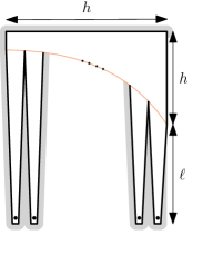
Figure 18: Construction of a simple polygon $P$ for which any $(t-\varepsilon)$-spanner has complexity $\Omega(n^{1+1/(t-1)})$. The shortest path from the $i$-th to the $j$-th site has complexity $|i-j|$.

To achieve a lower bound for $m>n$, we slightly adapt our polygon such that the top of each spike has complexity $\Theta(m/n)$. This implies that the path between $p_{i}$ and $p_{j}$ has complexity $m/n\cdot|i-j|$ instead. For this adapted polygon $P^{\prime}$, any spanning subgraph of $\vartheta_{n}$ of hop-diameter $h$ and total weight $w$ is in one-to-one correspondence to an $(h+1-\varepsilon)$-spanner of $P^{\prime}$ of complexity $\Theta(m/n\cdot w)$. It follows from Lemma 6.2 that any $(t-\varepsilon)$-spanner of $P^{\prime}$ has complexity $\Omega(m/n\cdot n^{1+1/(t-1)})=\Omega(mn^{1/(t-1)})$.

Corollary 6.3.

For any integer constant $t\geq 2$, there exists a set of $n$ point sites in a simple polygon $P$ with $m=\Omega(n)$ vertices for which any geodesic $t$-spanner has complexity $\Omega(mn^{1/t})$.

References

- [1] Mohammad Ali Abam, Marjan Adeli, Hamid Homapour, and Pooya Zafar Asadollahpoor. Geometric spanners for points inside a polygonal domain. In 31st International Symposium on Computational Geometry, SoCG, volume 34 of LIPIcs, pages 186–197, 2015.
- [2] Mohammad Ali Abam, Mark de Berg, Mohammad Farshi, Joachim Gudmundsson, and Michiel H. M. Smid. Geometric spanners for weighted point sets. Algorithmica, 61(1):207–225, 2011.
- [3] Mohammad Ali Abam, Mark de Berg, and Mohammad Javad Rezaei Seraji. Geodesic spanners for points on a polyhedral terrain. SIAM J. Comput., 48(6):1796–1810, 2019.
- [4] Sunil Arya, Gautam Das, David M. Mount, Jeffrey S. Salowe, and Michiel H. M. Smid. Euclidean spanners: short, thin, and lanky. In In Twenty-Seventh Annual ACM Symposium on Theory of Computing, STOC, Proceedings, pages 489–498. ACM, 1995.
- [5] Michael A. Bender and Martin Farach-Colton. The LCA problem revisited. In In Theoretical Informatics, 4th Latin American Symposium, LATIN, Proceedings, volume 1776 of Lecture Notes in Computer Science, pages 88–94. Springer, 2000.
- [6] Sujoy Bhore and Csaba D. Tóth. Euclidean Steiner spanners: Light and sparse. SIAM Journal on Discrete Mathematics, 36(3):2411–2444, 2022.
- [7] Prosenjit Bose, Jurek Czyzowicz, Evangelos Kranakis, Danny Krizanc, and Anil Maheshwari. Polygon cutting: Revisited. In Discrete and Computational Geometry, Japanese Conference, JCDCG, Revised Papers, volume 1763 of LNCS, pages 81–92, 1998.
- [8] Prosenjit Bose, Rolf Fagerberg, André van Renssen, and Sander Verdonschot. On plane constrained bounded-degree spanners. Algorithmica, 81(4):1392–1415, 2019.
- [9] Prosenjit Bose, Joachim Gudmundsson, and Michiel H. M. Smid. Constructing plane spanners of bounded degree and low weight. Algorithmica, 42(3-4):249–264, 2005.
- [10] Prosenjit Bose and J. Mark Keil. On the stretch factor of the constrained Delaunay triangulation. In In the 3rd International Symposium on Voronoi Diagrams in Science and Engineering, ISVD, pages 25–31. IEEE Computer Society, 2006.
- [11] Prosenjit Bose and Michiel H. M. Smid. On plane geometric spanners: A survey and open problems. Comput. Geom., 46(7):818–830, 2013.
- [12] Prosenjit Bose and André van Renssen. Spanning properties of Yao and -graphs in the presence of constraints. Int. J. Comput. Geom. Appl., 29(2):95–120, 2019.
- [13] T.-H. Hubert Chan, Anupam Gupta, Bruce M. Maggs, and Shuheng Zhou. On hierarchical routing in doubling metrics. ACM Trans. Algorithms, 12(4):55:1–55:22, 2016.
- [14] T.-H. Hubert Chan, Mingfei Li, Li Ning, and Shay Solomon. New doubling spanners: Better and simpler. SIAM J. Comput., 44(1):37–53, 2015.
- [15] Bernard Chazelle. Triangulating a simple polygon in linear time. Discret. Comput. Geom., 6:485–524, 1991.
- [16] Kenneth L. Clarkson. Approximation algorithms for shortest path motion planning. In Alfred V. Aho, editor, In the 19th Annual ACM Symposium on Theory of Computing, STOC, pages 56–65. ACM, 1987.
- [17] Gautam Das. The visibility graph contains a bounded-degree spanner. In In the 9th Canadian Conference on Computational Geometry, CCCG, 1997.
- [18] Mark de Berg, Otfried Cheong, Marc J. van Kreveld, and Mark H. Overmars. Computational geometry: Algorithms and applications, 3rd Edition. Springer, 2008. URL: https://www.worldcat.org/oclc/227584184.
- [19] Yefim Dinitz, Michael Elkin, and Shay Solomon. Shallow-low-light trees, and tight lower bounds for Euclidean spanners. In 49th Annual IEEE Symposium on Foundations of Computer Science, FOCS, pages 519–528, 2008.
- [20] Michael Elkin and Shay Solomon. Optimal Euclidean spanners: Really short, thin, and lanky. J. ACM, 62(5):35:1–35:45, 2015.
- [21] Subir Kumar Ghosh. Computing the visibility polygon from a convex set and related problems. J. Algorithms, 12(1):75–95, 1991.
- [22] Lee-Ad Gottlieb and Liam Roditty. An optimal dynamic spanner for doubling metric spaces. In 16th Annual European Symposium on Algorithms, ESA, volume 5193 of Lecture Notes in Computer Science, pages 478–489, 2008.
- [23] Leonidas J. Guibas and John Hershberger. Optimal shortest path queries in a simple polygon. J. Comput. Syst. Sci., 39(2):126–152, 1989.
- [24] Leonidas J. Guibas, John Hershberger, Daniel Leven, Micha Sharir, and Robert Endre Tarjan. Linear-time algorithms for visibility and shortest path problems inside triangulated simple polygons. Algorithmica, 2:209–233, 1987.
- [25] Sariel Har-Peled and Manor Mendel. Fast construction of nets in low-dimensional metrics and their applications. SIAM J. Comput., 35(5):1148–1184, 2006.
- [26] John Hershberger and Jack Snoeyink. Computing minimum length paths of a given homotopy class. Comput. Geom., 4:63–97, 1994.
- [27] John Hershberger and Subhash Suri. An optimal algorithm for Euclidean shortest paths in the plane. SIAM J. Comput., 28(6):2215–2256, 1999.
- [28] David G. Kirkpatrick. Optimal search in planar subdivisions. SIAM J. Comput., 12(1):28–35, 1983.
- [29] Hung Le and Shay Solomon. Truly optimal Euclidean spanners. In 60th IEEE Annual Symposium on Foundations of Computer Science, FOCS, pages 1078–1100. IEEE Computer Society, 2019.
- [30] Christos Levcopoulos, Giri Narasimhan, and Michiel H. M. Smid. Efficient algorithms for constructing fault-tolerant geometric spanners. In In the 13th Annual ACM Symposium on the Theory of Computing, STOC, Proceedings, pages 186–195. ACM, 1998.
- [31] Richard J. Lipton and Robert Endre Tarjan. A separator theorem for planar graphs. SIAM Journal on Applied Mathematics, 36(2):177–189, 1979.
- [32] Joseph S. B. Mitchell and Wolfgang Mulzer. Proximity algorithms. In Handbook of Discrete and Computational Geometry (3rd Edition), chapter 32, pages 849–874. Chapman & Hall/CRC, 2017.
- [33] Joseph S. B. Mitchell, Christine D. Piatko, and Esther M. Arkin. Computing a shortest k-link path in a polygon. In 33rd Annual Symposium on Foundations of Computer Science, FOCS, pages 573–582. IEEE Computer Society, 1992.
- [34] Joseph S. B. Mitchell, Günter Rote, and Gerhard J. Woeginger. Minimum-link paths among obstacles in the plane. Algorithmica, 8(5&6):431–459, 1992.
- [35] Giri Narasimhan and Michiel H. M. Smid. Geometric Spanner Networks. Cambridge University Press, 2007.
- [36] Subhash Suri. A linear time algorithm for minimum link paths inside a simple polygon. Computer Vision, Graphics, and Image Processing, 35(1):99–110, 1986.
- [37] Haitao Wang. A new algorithm for Euclidean shortest paths in the plane. In 53rd Annual ACM SIGACT Symposium on Theory of Computing, STOC, pages 975–988. ACM, 2021.