tiny[table]font=tiny

Resolving the stellar-collapse and hierarchical-merger origins of the coalescing black holes

Abstract

Spin and mass properties provide essential clues in distinguishing the formation channels for coalescing binary black holes (BBHs). With a dedicated non-parametric population model for the joint distributions of mass, spin magnitude, and spin orientation of the black holes (BHs) in the coalescing binaries, we find two distinct categories of BHs among the GWTC-3 events with considerably different spin and mass distributions. One category, with a mass ranging from $\sim 25M_{\odot}$ to $\sim 80M_{\odot}$, is distinguished by the high spin-magnitudes and consistent with the (hierarchical) merger origin. The other category, characterized by low spins, has a sharp mass cutoff at $\sim 40M_{\odot}$ ($<56.8M_{\odot}$ at 90% credible level), which is natural for the stellar-collapse origin. In particular, such a mass cutoff is expected for the pair-instability explosion of massive stars. The stellar-collapse category is estimated to consist of $\sim 70\%$ filed binaries and $\sim 30\%$ dynamical assembly from star clusters (mostly globular clusters); while the merger-origin category may contain comparable amounts of events from the Active Galactic Nuclei disks and star clusters.

Yin-Jie Li¹, Yuan-Zhu Wang¹, Shao-Peng Tang¹, Yi-Zhong Fan^1,2.

Key Laboratory of Dark Matter and Space Astronomy, Purple Mountain Observatory, Chinese Academy of Sciences, Nanjing 210008, China

School of Astronomy and Space Science, University of Science and Technology of China, Hefei 230026, China

Thanks to the excellent performance of the LIGO/Virgo network, about $90$ gravitational wave (GW) events have been detected so far, and most of them are coalescing binary black holes (BBHs) [1, 2, 3, 4]. The astrophysical origins of these binaries, however, are still under debate. In the literature there are two popular scenarios: field and dynamical [5, 6]. The field BBHs are formed from isolated stellar binaries, while the dynamical assembly is formed through interactions in dense stellar environments, like star clusters and the accretion disks of Active Galactic Nuclei (AGN) [5, 6, 7]. The stellar-origin BHs are expected to be absent in the so-called upper-mass gap (UMG) as a result of the (pulsational) pair-instability supernova ((P)PISN) explosions [8, 9], and the UMG is widely anticipated to start at $\sim 40-55~{}M_{\odot}$, though the threshold may be shifted under some special circumstances [10, 11, 12, 9, 13, 14, 15]. By contrast, merger-formed BHs may populate the UMG and contribute to hierarchical mergers via dynamical formation channel [7, 16, 5, 6]. Moreover, merger-formed BHs are distinguishable from those born in stellar explosions for their high spin magnitudes (with a typical value of $\sim 0.7$) [17, 18]. Therefore, it is possible to distinguish the category of higher-generation (HG) BHs via analyzing the joint distribution of mass and spin for BBHs from GW observations, and simultaneously constrain the lower-edge of the UMG. There have been dedicated efforts made, but it is still unclear whether there is a UMG and a distinct HG category within the current GW data [19, 20, 21, 22, 23, 24, 25, 26]. To reliably clarify the situation, here we propose a non-parametric population model with minimal assumptions to explore the underlying categories/groups of the coalescing BHs.

In our approach, there are two key points. First, the component masses and spins in a BBH system are independently drawn from the same underlying distribution (see also ref.[27] for the similar parameterization of the mass function of BBHs). This is because the two BHs in a binary system may go through the same evolutionary processes, such as the (P)PISN explosions [8, 9]; thus, the features in the distributions of the two components may be similar. What’s more, the mass ratio reversal makes it difficult to judge which objects formed first in field binaries [28]; therefore, it is reasonable to have the two component BHs follow the same distribution. Second, our model incorporates a joint mass-spin distribution, which makes it suitable to clarify the correlations between the mass distribution and spin distribution of the BHs. Since coalescing BHs from diverse formation channels may have different mass and spin distributions, we incorporate $N$ components into the modeling, i.e.,

$$\pi(m,a,\cos\theta|{\bf\Lambda})=\pi_{1}(m,a,\cos\theta|{\bf\Lambda}_{1})\times(1-\sum_{i=1}^{N}{r_{i}})+\sum_{i=2}^{N}{\pi_{i}(m,a,\cos\theta|{\bf\Lambda}_{i})\times r_{i}},$$ (1)

where $m$, $a$, and $\cos\theta$ are the mass, spin magnitude, and cosine tilt angle of spin orientation for the BHs, respectively; and $r_{i}$ is the mixing fraction of the $i$-th component (the sum of $r_{i}$ satisfies the condition of $\sum_{i=2}^{N}{r_{i}}<1$). The joint distribution of masses and spins for the $i$-th component reads

$$\pi_{i}(m,a,\cos\theta|{\bf\Lambda}_{i}) =\mathcal{PS}(m|\alpha_{i},m_{{\rm min},i},m_{{\rm max},i},\delta_{i},f_{i}(m;\{f_{i}^{j}\}_{j=0}^{N_{\rm knot}}))$$ (2)

$$\times\mathcal{G}(a|a_{{\rm min},i},a_{{\rm max},i},\mu_{a,i},\sigma_{a,i})\times\mathcal{GU}(\cos\theta|z_{{\rm min},i},\zeta_{i},\sigma_{{\rm z,}i}),$$

where $\mathcal{PS}$ is the one-dimension PowerLawSpline model for the BBH primary mass function by Edelman et al.[29]. This non-parametric model is flexible in determining the underlying mass distributions of the BHs in different categories if distinguishable; $f_{i}(m)$ is the cubic-spline perturbation function interpolated between ${N_{\rm knot}}$ knots placed in the mass range. We fix the locations of each knot to be linear in the logarithm space within [5, 100] $M_{\odot}$ and restrict the perturbation to zero at the minimum and maximum knots. For simplicity, we use 15 knots to interpolate the perturbation function $f_{i}$, which is enough to characterize the mass distribution in detail[29], and we adopt a ‘conservative’ prior width as $\sigma_{\rm knot}=1$ for each specified knot. $\mathcal{G}$ is a truncated Gaussian within the range of [$a_{{\rm min},i}$, $a_{{\rm max},i}$] with a central value and a standard deviation of $\mu_{a,i}$ and $\sigma_{a,i}$. The $\cos\theta$ distribution is a combination of isotropic-spin (characterized by $\mathcal{U}$) and nearly aligned (characterized by $\mathcal{G}$) assemblies, i.e.,

$$\mathcal{GU}(\cos\theta|z_{{\rm min},i},\zeta_{i},\sigma_{{\rm z,}i})=\mathcal{G}(\cos\theta|z_{{\rm min},i},1,1,\sigma_{z,i})\times\zeta_{i}+(1-\zeta_{i})\times\mathcal{U}(\cos\theta|-1,1),$$ (3)

where $\mathcal{U}$ is the uniform distribution between $-1$ and 1. Note that there is a lower cutoff ($z_{{\rm min},i}$) in the nearly aligned assembly (but not in the isotropic-spin assembly). Following ref.[27], the two-component masses are paired by $(m_{2}/m_{1})^{\beta}$. Therefore, the final population model takes the form of

$$\pi(m_{1},m_{2},a_{1},a_{2},\cos\theta_{1},\cos\theta_{2}|{\bf\Lambda};\beta)\propto\pi(m_{1},a_{1},\cos\theta_{1}|{\bf\Lambda})\times\pi(m_{2},a_{2},\cos\theta_{2}|{\bf\Lambda})\times(m_{2}/m_{1})^{\beta}.$$ (4)

All the descriptions of the hyper-parameters are summarized in Tab. 1.

Results

We have performed inferences with our population models and made Bayesian model comparisons. It reveals two groups of BHs with significantly different spin distributions and mass distributions (see Fig.1), which are evidently illustrated by the posterior distributions of the observed events weighted by the population-informed priors obtained by our two-component model (see Fig.2). The two categories of BHs are clear and identifiable, and the absence of BHs with $m\gtrsim 50M_{\odot}$ and $a\lesssim 0.4$ indicates that hierarchical merger as a mechanism to populate the Pair-instability Mass Gap is legitimate [30].

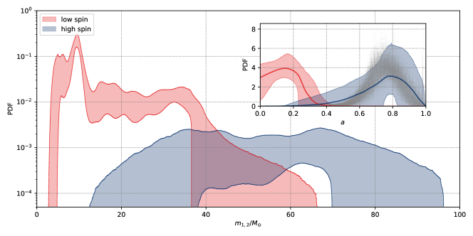
Figure 1: Reconstructed mass distribution of BHs for each group, and the shaded areas represent the $90\%$ credible regions. The inset is for the spin-magnitude distributions of the two groups and the final-spin distribution of the mergers from the LSG; the shaded areas and solid lines indicate the $90\%$ credible regions and mean values for the spin-magnitude distribution for each group, while the grey lines represent the final-spin distributions of the mergers from the LSG, which are calculated by the 500 independent posterior samples.

Two categories.

For the spin-magnitude distributions, the first group (hereafter the low-spin group; LSG) peaks at $0.14^{+0.11}_{-0.11}$ and terminates at $0.29_{-0.06}^{+0.34}$ (hereafter the values are for the median value and the 90% symmetry interval, unless otherwise noticed), while in the second group (hereafter the high-spin group; HSG), the spin-magnitude distribution starts at $0.44_{-0.29}^{+0.36}$, peaks at $0.79^{+0.15}_{-0.20}$ and ends at $0.94^{+0.05}_{-0.11}$. The significantly different spin-magnitude distributions between the two groups indicates the different physical origins [7]. For the mass distributions, the LSG (HSG) starts at $3.10^{+1.32}_{-0.9}M_{\odot}$ ($24.5^{+12.1}_{-17.8}M_{\odot}$) and terminates at $41.7^{+28.4}_{-5.1}M_{\odot}$ ($81^{+15.2}_{-11.2}M_{\odot}$) with an overall power-law index of $1.8^{+0.96}_{-0.89}$ ($-0.5^{+3.1}_{-2.7}$). The HSG takes a fraction of $0.04^{+0.02}_{-0.02}$ of all the coalescing BHs. The posterior of other parameters for the mass and spin distributions is displayed in the Supplementary Material. For the spin-orientation distributions, the LSG (HSG) has a fraction of $0.68^{+0.22}_{-0.25}$ ($0.50^{+0.35}_{-0.32}$) nearly-aligned assembly. And the lower cutoff of the $\cos\theta$ in the nearly-aligned assembly is estimated to be $z_{\rm min,1}=0.20^{+0.39}_{-0.64}$ ($z_{\rm min,2}=0.24^{+0.59}_{-0.94}$) for the LSG (HSG). In both groups, either the perfectly aligned (i.e., $\zeta_{i}=1$ & $z_{\rm min,i}\sim 1$) or the fully isotropic distribution (i.e., $\zeta_{i}=0$ or $z_{\rm min,i}=-1$ & $\sigma_{\rm z,i}\gg 1$) is disfavored, as shown in Fig. 3.

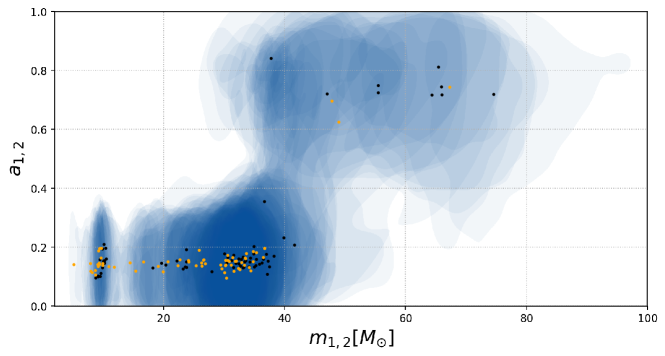
Figure 2: Posteriors of individual component masses and spin magnitudes of BBHs in GWTC-3, re-weighted to a population-informed prior inferred by the fiducial model. The shaded areas mark the $90\%$ credible regions and the black (orange) points stand for the mean values for the primary (secondary) BHs. The difference between the two groups is evident: the first group is lighter than $\sim 40M_{\odot}$ with spin magnitudes $\lesssim 0.3$, while the second group extends to the higher mass range and has a typical spin magnitude $\sim 0.75$.

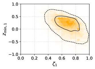
Figure 3: Posterior distribution for the mixing fraction $\zeta_{\rm i}$ and the minimum cutoff $z_{\rm min,i}$ of the nearly aligned assemblies in the first (left) and the second (right) components. The dashed and solid contours mark the central 50% and 90% posterior credible regions, respectively.

Evidence for Hierarchical mergers.

As shown in the insert of Fig. 1, the spin-magnitude distribution of HSG (blue dashed region) is well overlapped with the final-spin distribution of the first-generation BBHs (grey lines) . Note that we do not take into account the contribution of the HG BBHs to the final-spin distribution; otherwise, the peak will be slightly shifted to a higher value [16, 17], so it may be even more consistent with the spin-magnitude distribution of the HSG. In both the spin-magnitude distribution of the HSG and the final-spin distribution of the first-generation BBHs, the locations of peaks are slightly higher than 0.7, the typical value of the final-spin distribution for mergers in star clusters [17, 18]. This is because about half of the spin orientations of the dynamical assembly are nearly aligned to the orbital angular momentum vectors of the binaries as shown in Fig.3 (see also Supplementary Figure 3), which will enhance the final spin of the remnants as predicted by the dynamical formation in the AGN disks [16, 31]. What’s more, previous mergers containing HG BHs will also produce larger final spins [16, 17].

With the identification of the HSG as the HG category, we estimate that $0.03^{+0.04}_{-0.02}$ of the sources are hierarchical mergers containing at least one HG BH, and $0.02^{+0.02}_{-0.01}$ of the sources have two HG BHs (see Supplementary Figure 4). Assuming the merger rate of BBHs evolves with the redshift $z$ as $\propto(z+1)^{2.7}$, as obtained by Abbott et al. [20], we have a local merger rate density of $0.6^{+0.6}_{-0.3}~{}{\rm Gpc^{-3}yr^{-1}}$ for the hierarchical events. Additionally, we have identified events with probabilities $>50\%$ to be hierarchical mergers (as summarized in Supplementary Table 2). In particular, GW190521_030229, GW190602_175927, and GW191109_010717 have probabilities $>50\%$ to host double HG BHs.

Evidence for an upper-mass gap of stellar formed black holes.

Ignore the HG category; the remaining BHs (i.e., the LSG) were in the stellar-collapse category . There is a rapid decline after $\sim 40M_{\odot}$ in the mass function of the LSG, as shown in Fig. 1, which strongly supports the existence of the UMG caused by the (P)PISN [8, 9]. Indeed, we have $m_{\rm max,1}=39.04_{-3.57}^{+7.92}M_{\odot}$ (the $1\sigma$ minimal credible interval, as shown in Fig.4), which is in good agreement with the lower edge of the UMG predicted by stellar evolution [10, 11, 12].

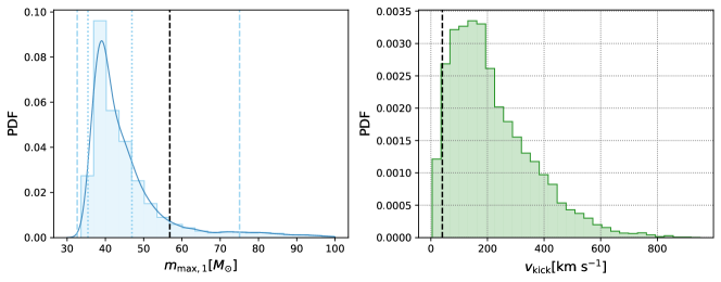
Figure 4: Posterior of the maximum-mass cutoff of the LSG (Left) and distribution of the kick velocities of the BBHs belonging to the dynamical assembly of the LSG (Right). On the left, the 68.3% ($1\sigma$) and 95.4% ($2\sigma$) minimal credible intervals are indicated by dashed and dotted lines; the black dashed line represents the position for 90% cumulative probability. On the right, we adopt the median values of the inferred parameters for calculations; the black dashed line marks the position for 1/20 cumulative probability, with kick velocities below which the remnants are likely retained in the host star clusters.

The multi-type of formation environments for dynamical captures.

According to our results, the isotropic-spin and nearly aligned assemblies are comparable in the HSG (see Fig. 3). Therefore, dynamical formation environments like AGN disks (that produce nearly aligned binaries [33, 16]) and star clusters (that produce binaries with isotropic spin orientation [34, 35]) might contribute equally to the hierarchical mergers [7]. Yang et al.[16] suggests that in AGN disks, the fraction of first-generation mergers is $\lesssim 50\%$, so considering the fraction of hierarchical mergers in the whole population (i.e., $\sim 3\%$ as we obtained), the mergers from AGN disks take a negligible fraction in the LSG. Therefore in the whole BBH population, a fraction of $\sim 66\%$ (i.e., the near-aligned BHs in the LSG) may originate from the evolution of the field binaries, such as the common-envelope evolution [36, 37] and the chemically homogeneous evolution [38, 39, 40], and the rest (i.e., $\sim 31\%$) are the dynamical assembly from the star clusters[41, 42].

The escape speed of the environment plays a crucial role in generating hierarchical mergers[43], since the HG BBHs can be formed only if the remnants of previous mergers are efficiently retained within their host. Based on our analysis, the proportion between first-generation mergers and hierarchical mergers of dynamical assembly in star clusters is $\sim 1/20$. With the distribution of the kick velocities for the isotropic-spin assembly in the LSG, we find that the average escape velocity of $40.5~{}{\rm km~{}s^{-1}}$ for the host star clusters can keep $\sim 1/20$ of the remnants retained in the host star clusters (see right panel of Fig. 4). Compared to the distributions of the escape velocities of the observed globular clusters and nuclear clusters [44], we suggest that the globular clusters, rather than the nuclear star clusters, dominate the local merger rate of dynamically formed BBHs.

Discussion With a flexible population model incorporating a joint mass-spin distribution of the BHs, we find strong evidence for the widely discussed hierarchical mergers [7] and the Pair-instability Mass Gap [45, 46]. The Advanced LIGO/Virgo/KAGRA network will have higher sensitivities and longer duration in the future runs [47], so the BBH sample will increase rapidly in the next decade and the maximum-mass cutoff of the stellar-collapse category (i.e., $m_{\rm max,1}$) in a given red-shift bin will be reasonably measured. Such a data set can be used to probe the possible evolution of the $m_{\rm max,1}$, and hence the metallicity, with the age of the universe [14]. Additionally, such an evolution in the mass distribution of the stellar-collapse category (if significant) can also contribute to cosmology via ’spectrum siren’ [48], hence one can obtain a percent-level measurement of the Hubble expansion $H(z)$ at $z\lesssim 1$ with Advanced LIGO/Virgo [49]. And the measurement uncertainty of $H(z)$ can even reach $\lesssim 1\%$ at $z\gtrsim 2$ with the contribution of the neutron star mass function [50] in the era of Cosmic Explorer and Einstein Telescope [48], which would be sufficiently accurate to resolve the so-called Hubble tension [51]. A rapidly growing BBH sample is also needed to accurately infer the fractions of dynamical mergers from different formation environments, which have just been loosely constrained by the current gravitational wave data within out work.

Methods

Hierarchical Bayesian inference.

Following Abbott et al.[20], we use the data of BBHs from GWTC-3 [1, 2, 3, 4], and adopt a false-alarm rate (FAR) of $1yr^{-1}$ as the threshold to select the events. What’s more, GW190814 is excluded from the analysis, because it is a significant outlier [20, 52] in the BBH populations, and may be associated with neutron star$-$BH binary systems [53]. Therefore in total, there are 69 events selected for our analysis. The posterior samples for each BBH event are adopted from the Gravitational Wave Open Science Center (https://www.gw-openscience.org/eventapi/html/GWTC/).

We perform hierarchical Bayesian inferences to fit the data of the observed events {d} with the population models. Following the framework described in ref.[54, 20], the likelihood of the hyperparameters $\boldsymbol{\Lambda}$, given data $\{d\}$ from $N_{\rm det}$ GW detections, can be expressed as

$$\mathcal{L}(\{d\}|\boldsymbol{\Lambda})\propto N^{N_{\rm det}}e^{-N{\xi(\boldsymbol{\Lambda})}}\prod_{i=1}^{N_{\rm det}}\int{\mathcal{L}(d_{i}|\theta_{i})\pi(\theta_{i}|\boldsymbol{\Lambda})d\theta_{i}},$$ (5)

where $N$ is the number of mergers in the Universe over the observation period, which is related to the merger rate, and $\xi(\boldsymbol{\Lambda})$ means the detection fraction, The single-event likelihood $\mathcal{L}(d_{i}|\theta_{i})$ can be estimated using the posterior samples (see ref.[54] for the detail), and $\xi(\boldsymbol{\Lambda})$ is estimated using a Monte Carlo integral over detected injections as introduced in the Appendix of ref.[54]. The injection campaigns can be adopted from https://doi.org/10.5281/zenodo.5546676, where they combine O1, O2, and O3 injection sets, ensuring a constant rate of injections across the total observing time. For simplicity, we assume that the merger rate density increases with redshift, i.e., $\mathcal{R}\propto(1+z)^{2.7}$, as reported in Abbott et al. [20]. The priors of all the parameters are summarized in Tab. 1. To check the reliability of our model and the validation of the findings, we also introduce some other population models for comparison, like PS&DoubleSpin, and PS&LinearCorrelation (as defined below). In this work, we apply the sampler Pymultinest [55] to obtain the posterior of the hierarchical hyperparameters.

Table 1: Hyperparameters and Priors for the fiducial models and PS&LinearCorrelation model

descriptions	parameters	priors
		1st component	2nd/3th component
slope index of the mass function	$\alpha_{i}$	U(-4,8)	U(-4,8)
smooth scale of the $i$-th mass lower edge	$\delta_{i}$	U(1,10)	U(1,10)
minimum mass of the $i$-th mass function	$m_{{\rm min},i}[M_{\odot}]$	U(2,60)	U(2,60)
maximum mass of the $i$-th mass function	$m_{{\rm max},i}[M_{\odot}]$	U(20,100)	U(20,100)
interpolation values of perturbation for $i$-th mass function	$\{f_{i}^{j}\}_{j=1}^{15}$	$\mathcal{N}(0,1)$	$\mathcal{N}(0,1)$
Mass Constraints		$m_{{\rm max},i}-m_{{\rm min},i}>10M_{\odot}$
mean of $a$ distribution in $i$-th component	$\mu_{{\rm a},i}$	U(0,1)	U(0,1)
standard deviation of $a$ distribution in $i$-th component	$\sigma_{{\rm a},i}$	U(0.02, 0.5)	U(0.02, 0.5)
minimum value of $a$ distribution in $i$-th component	$a_{{\rm min},i}$	0	U(0,0.8)
maximum value of $a$ distribution in $i$-th component	$a_{{\rm max},i}$	U(0,1)	U(0,1)
Spin Constraints		$a_{{\rm max},i}>\mu_{{\rm a},i}>a_{{\rm min},i}$
standard deviation of nearly aligned $\cos\theta$ in $i$-th component	$\sigma_{{\rm z},i}$	U(0.1, 4)	U(0.1, 4)
minimum $\cos\theta$ of nearly aligned assembly in $i$-th component	$z_{{\rm min},i}$	U(-1,0.9)	U(-1,0.9)
mixing fraction of nearly aligned assembly in $i$-th component	$\zeta_{i}$	U(0,1)	U(0,1)
mixing fraction of the $i$-th component	$r_{i}$	U(0,1)
Constraint		$\sum_{i=2}^{N}{r_{i}}<1$
pairing function	$\beta$	U(0,8)
local merger rate density	${\rm log}_{10}R_{0}[{\rm Gpc^{-3}yr^{-1}}]$	U(0,3)
Parameters For PS&LinearCorrelation
$\sigma_{\rm a}$ at the lower-mass edge	$\sigma_{\rm a}^{\rm left}$	U(0.02,0.5)
$\sigma_{\rm a}$ at the higher-mass edge	$\sigma_{\rm a}^{\rm right}$	U(0.02,0.5)
$\mu_{\rm a}$ at the lower-mass edge	$\mu_{\rm a}^{\rm left}$	U(0,1)
$\mu_{\rm a}$ at the higher-mass edge	$\mu_{\rm a}^{\rm right}$	U(0,1)
standard deviation of the $\cos\theta$ distribution	$\sigma_{{\rm z}}$	U(0.1, 4)
lower cutoff of the $\cos\theta$ distribution in nearly aligned assembly	$z_{{\rm min}}$	U(-1,0.9)
mixing fraction of the nearly aligned assembly	$\zeta$	U(0,1)

• Note. Here, ‘U’ means the uniform distribution and ‘$\mathcal{N}$’ means the normal distribution.

Model comparison

Table 2: Model comparison results

Models	$\ln{\mathcal{B}}$
two-component	0
three-component	-1.1
two-component ($z_{{\rm min},i}=-1$)	-2.7
PS&LinearCorrelation	-6.3
PS&DoubleSpin	-10.3
Single-component	-11.5
PS&DefaultSpin	-14.1
PP&DefaultSpin	-19.7

Note: these log Bayes factors are relative to the two-component model.

For context, $\ln\mathcal{B}>2.3$ ($\ln\mathcal{B}>3.5$) can be interpreted as a strong (very strong) preference for one model over another, and $\ln\mathcal{B}>4.6$ as decisive evidence [56]. We perform inferences with a single component, two components, and three components, respectively, and find the two-component model can better fit the current GW data, as summarized in Tab. 2. The three-component model has lower evidence than the two-component model, and the distributions of the second and third components are highly degenerate. Therefore the third component is not required by current data. Additionally, we have also performed an inference without the lower cutoff of $\cos\theta$ in the nearly aligned assemblies (i.e., $z_{\rm min,i}=-1$), which is less favored by a log Bayes factor of $\ln\mathcal{B}=-2.7$ compared to the fiducial model, so our parameterization of the $\cos\theta$ distribution is reliable. We further compare the two-component model to other models in order to find out whether the two components adopted in the modeling are indeed necessary, and finally, all of the other alternative models are disfavored (see below for details).

Only one peak in the spin-magnitude distribution?

We first compare the two-component model to the other models with only one peak in the spin-magnitude distribution, i.e., PS&DefaultSpin and PP&DefaultSpin adopted in Abbott et al.[20], where the spin distribution and the mass functions are those of the Default model and the PS / PP model in Abbott et al.[20]. Note that in their PS model, the secondary mass distribution follows $m_{2}^{\beta_{\rm q}}$ conditioned by $m_{1}$, where ${\beta_{\rm q}}$ is the power law index of the mass ratio distribution. As shown in Tab.2, the PS&DefaultSpin, and the PP&DefaultSpin are definitively disfavored by the log Bayes factors of $\ln\mathcal{B}=-14.1$, and $\ln\mathcal{B}=-19.7$, respectively.

PS&DoubleSpin: Is double-peak spin-magnitude distribution uncorrelated with the mass distribution?

We have found that double peaks in the spin-magnitude distribution are required, but are they still consistent in the whole mass range? To answer this question, we carry out another inference with the PS&DoubleSpin model, where the mass distribution (i.e., PS model adopted from Abbott et al. [20]) and the spin distribution (i.e., DoubleSpin) are constructed independently. For the spin distribution, we apply two components to catch the underlying peaks; therefore the DoubleSpin model reads

$$\pi(a,\cos\theta|{\bf\Lambda})=\pi_{1}(a,\cos\theta|{\bf\Lambda}_{1})\times(1-r_{2})+\pi_{2}(a,\cos\theta|{\bf\Lambda}_{2})\times r_{2},$$ (6)

where $r_{2}$ is the mixing fraction of the secondary component, and the spin distribution of $i$-th component is

$$\pi_{i}(a,\cos\theta|{\bf\Lambda}_{i})=\mathcal{G}(a|a_{{\rm min},i},a_{{\rm max},i},\mu_{a,i},\sigma_{a,i})\times\mathcal{GU}(\cos\theta|z_{{\rm min},i},\zeta_{i},\sigma_{{\rm z,}i}),$$ (7)

where $\mathcal{G}$ and $\mathcal{GU}$ are the same as those in the main text. Then the spin distribution of the BBHs should be

$$\pi(a_{1},a_{2},\cos\theta_{1},\cos\theta_{2}|{\bf\Lambda})=\pi(a_{1},\cos\theta_{1}|{\bf\Lambda})\times\pi(a_{2},\cos\theta_{2}|{\bf\Lambda}).$$ (8)

The priors of the spin model are the same as those summarized in Tab.1. We find that the PS&DoubleSpin is disfavored by a log Bayes factor of $\ln\mathcal{B}=-10.3$ compared to the two-component model, but is slightly better than the single-component model (see Tab.2). We therefore conclude that, for coalescing BBHs, the spin distribution is not independent of but correlated with the mass distribution.

PS&LinearCorrelation: Is spin-magnitude distribution linearly changed with the mass distribution?

As we have found that the spin-magnitude distribution is not consistent in the whole mass range, then does the spin-magnitude distribution gradually change as the mass increases? So we introduce a mass-spin distribution where the spin-magnitude distribution (i.e., LinearCorrelation) linearly correlates with the mass distribution (i.e., PS adopted from Abbott et al. [20]). Therefore, the PS&LinearCorrelation model reads

$$\pi(a,\cos\theta|m,{\bf\Lambda})=\mathcal{G}(a|0,1,\mu_{a}(m),\sigma_{a}(m))\times\mathcal{GU}(\cos\theta|z_{{\rm min}},\zeta,\sigma_{{\rm z}}),$$ (9)

where $\mu_{a}(m)$ and $\sigma_{a}(m)$ are the linear function of the component mass $m$,

$$\mu_{a}(m)=\frac{(m-m_{\rm min})\mu_{\rm a}^{\rm right}+(m_{\rm max}-m)\mu_{\rm a}^{\rm left}}{m_{\rm max}-m_{\rm min}},$$ (10)

$$\sigma_{a}(m)=\frac{(m-m_{\rm min})\sigma_{\rm a}^{\rm right}+(m_{\rm max}-m)\sigma_{\rm a}^{\rm left}}{m_{\rm max}-m_{\rm min}}.$$

where the priors and the descriptions of the hyperparameters for the model are summarized in Table 1. We find that the PS&LinearCorrelation model is disfavored by a log Bayes factor of $\ln\mathcal{B}={-6.3}$ compared to the two-component model. Therefore the spin-magnitude distribution does not linearly change with the masses of the BHs, though we find that $\mu_{\rm a}^{\rm right}>\mu_{\rm a}^{\rm left}$ at 99% credible level and $\sigma_{\rm a}^{\rm right}>\sigma_{\rm a}^{\rm left}$ at 93% credible level (see Supplementary Figure 1), which means that the heavier BHs have larger spin magnitude, and the spin-magnitude distribution broadens with the increasing mass.

In view of the above facts, we conclude that there are two distinct groups in the mass and spin distributions of coalescing BHs.

The codes (Bilby and PyMultiNest) used in this analysis are standard in the community.

The GW data used in this work are adopted from the Gravitational Wave Open Science Center (https://www.gw-openscience.org/eventapi/html/GWTC/). The injection campaigns used for calculating selection effects are adopted from (https://doi.org/10.5281/zenodo.5546676).

This work was supported in part by NSFC under grants of No. 12233011, No. 11921003, and No. 12203101. This research has made use of data and software obtained from the Gravitational Wave Open Science Center (https://www.gw-openscience.org), a service of LIGO Laboratory, the LIGO Scientific Collaboration and the Virgo Collaboration. LIGO is funded by the U.S. National Science Foundation. Virgo is funded by the French Centre National de Recherche Scientifique (CNRS), the Italian Istituto Nazionale della Fisica Nucleare (INFN) and the Dutch Nikhef, with contributions by Polish and Hungarian institutes.

Y.Z.F, Y.J.L, and Y.Z.W launched the project. Y.J.L carried out the data analysis. All authors joined the discussion and prepared the paper.

Correspondence and requests for materials should be addressed to Y.Z.F (yzfan@pmo.ac.cn).

Supplementary Information

The posterior distributions

The posteriors distribution of the hyperparameters describing the mass distributions and the spin distributions introduced in the main text are displayed in Supplementary Figure 2 and Supplementary Figure 3, respectively.

The branch ratios of the two categories

Using the results from the fiducial model in the main text, we calculate the fractions of the BBH mergers with component BHs belonging to the two categories (see Supplementary Figure 4). We find $0.97^{+0.02}_{-0.04}$ of the sources have both components in the LSG, while $0.02^{+0.02}_{-0.01}$ have the primary components in the HSG, and $0.02^{+0.02}_{-0.01}$ have both components in the HSG. We assume that the HSG is made of HG BHs, then $0.03^{+0.04}_{-0.02}$ of the sources are hierarchical mergers, which is consistent with the results in Wang et al. 2022[1] where an astrophysical-motivated model was used. We further calculate the local merger rate density of the sources including at least one high-spin component to be $0.6^{+0.6}_{-0.3}~{}{\rm Gpc^{-3}yr^{-1}}$.

Possible hierarchical mergers.

We also calculate the probabilities for each BBH event that belongs to a specific combination of the categories, and select the events with probabilities of $>0.5$ to contain at least one BH belonging to the high-spin category. The results are summarized in Supplementary Table 1.

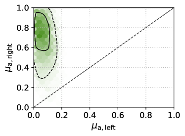
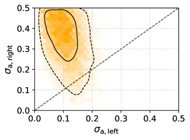
Supplementary Figure 1: Posterior distribution of $\mu_{\rm a}^{\rm right}$ vs. $\mu_{\rm a}^{\rm left}$ (left) and $\sigma_{\rm a}^{\rm right}$ vs. $\sigma_{\rm a}^{\rm left}$ (right). The dashed and solid contours mark the central 50% and 90% posterior credible regions, respectively. It turns out that $\mu_{\rm a}^{\rm right}>\mu_{\rm a}^{\rm left}$ at 99% credible level and $\sigma_{\rm a}^{\rm right}>\sigma_{\rm a}^{\rm left}$ at 93% credible level.

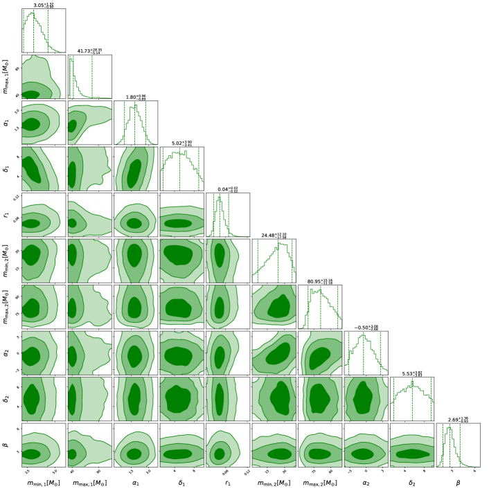
Supplementary Figure 2: Posterior distribution of all the parameters describing the mass distribution; the dashed lines in the marginal distribution represent the $90\%$ credible intervals.

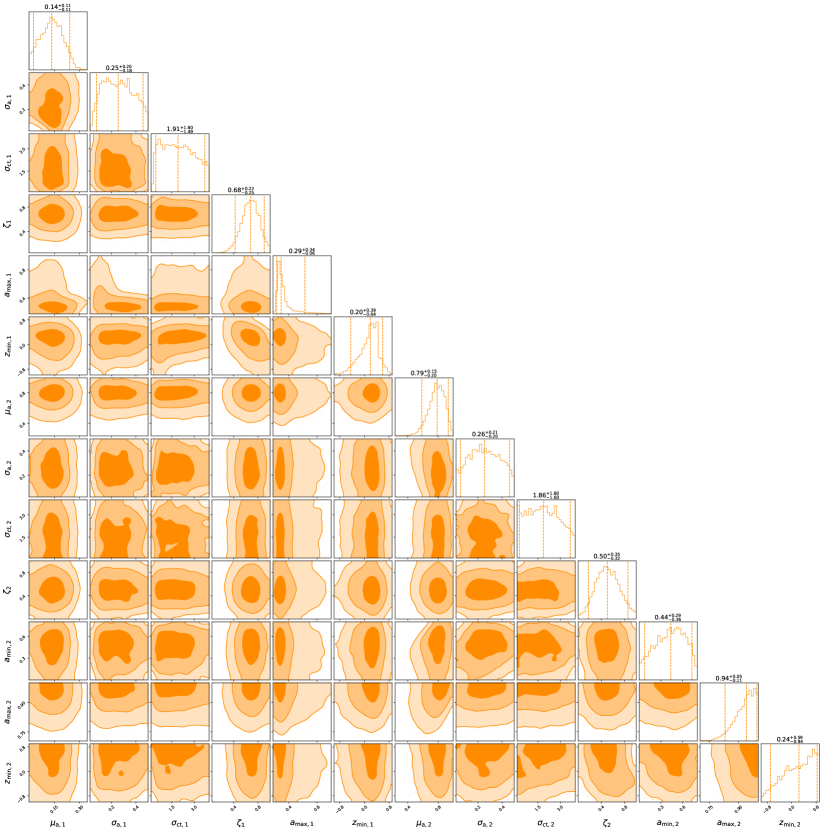
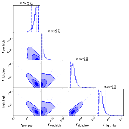
Supplementary Figure 3: Posterior distribution of all the parameters describing the spin distribution; the dashed lines in the marginal distribution represent the $90\%$ credible intervals.

Supplementary Figure 4: Distribution of the branch ratios for the BBHs with the primary and secondary objects belonging to the LSG and HSG. The dashed lines represent the 90% credible intervals

Supplementary Table 1. Probabilities of some events belonging to a specific category.
Events low+low low+high high+low high+high GW170729_185629 0.291 0.03 0.614 0.065 GW190517_055101 0.004 0.029 0.87 0.098 GW190519_153544 0.005 0.013 0.68 0.302 GW190521_030229 0.015 0.061 0.017 0.906 GW190602_175927 0.014 0.021 0.405 0.561 GW190620_030421 0.009 0.02 0.808 0.163 GW190701_203306 0.135 0.023 0.651 0.191 GW190706_222641 0.006 0.009 0.692 0.293 GW190929_012149 0.15 0.024 0.742 0.083 GW190805_211137 0.456 0.065 0.408 0.072 GW191109_010717 0.011 0.003 0.426 0.561 GW191230_180458 0.459 0.043 0.431 0.067 Note: Here ‘low+high’ means the primary object belong to the LSG while the secondary object belong to the HSG. We only display events with probabilities of low+low less than 0.5.

References

- [1] Abbott, B. P., Abbott, R. & Abbott, T. D. GWTC-1: A Gravitational-Wave Transient Catalog of Compact Binary Mergers Observed by LIGO and Virgo during the First and Second Observing Runs. Physical Review X 9, 031040 (2019). 1811.12907.
- [2] Abbott, R., Abbott, T. D. & Abraham, S. GWTC-2: Compact Binary Coalescences Observed by LIGO and Virgo during the First Half of the Third Observing Run. Physical Review X 11, 021053 (2021). 2010.14527.
- [3] Abbott, R., Abbott, T. D. & Acernese, F. GWTC-2.1: Deep Extended Catalog of Compact Binary Coalescences Observed by LIGO and Virgo During the First Half of the Third Observing Run. arXiv e-prints arXiv:2108.01045 (2021). 2108.01045.
- [4] Abbott, R., Abbott, T. D. & Acernese, F. GWTC-3: Compact Binary Coalescences Observed by LIGO and Virgo During the Second Part of the Third Observing Run. arXiv e-prints arXiv:2111.03606 (2021). 2111.03606.
- [5] Mandel, I. & Farmer, A. Merging stellar-mass binary black holes. Phys. Rep. 955, 1–24 (2022). 1806.05820.
- [6] Mandel, I. & Broekgaarden, F. S. Rates of compact object coalescences. Living Reviews in Relativity 25, 1 (2022). 2107.14239.
- [7] Gerosa, D. & Fishbach, M. Hierarchical mergers of stellar-mass black holes and their gravitational-wave signatures. Nature Astronomy 5, 749–760 (2021). 2105.03439.
- [8] Woosley, S. E. Pulsational Pair-instability Supernovae. Astrophys. J. 836, 244 (2017). 1608.08939.
- [9] Woosley, S. E. & Heger, A. The Pair-instability Mass Gap for Black Holes. Astrophys. J. Lett. 912, L31 (2021). 2103.07933.
- [10] Farmer, R., Renzo, M., de Mink, S. E., Marchant, P. & Justham, S. Mind the Gap: The Location of the Lower Edge of the Pair-instability Supernova Black Hole Mass Gap. Astrophys. J. 887, 53 (2019). 1910.12874.
- [11] Farmer, R., Renzo, M., de Mink, S. E., Fishbach, M. & Justham, S. Constraints from Gravitational-wave Detections of Binary Black Hole Mergers on the 12C(, )16O Rate. Astrophys. J. Lett. 902, L36 (2020). 2006.06678.
- [12] Renzo, M. et al. Sensitivity of the lower edge of the pair-instability black hole mass gap to the treatment of time-dependent convection. MNRAS 493, 4333–4341 (2020). 2002.08200.
- [13] Belczynski, K. et al. The Formation of a 70 M⊙ Black Hole at High Metallicity. Astrophys. J. 890, 113 (2020). 1911.12357.
- [14] Vink, J. S., Higgins, E. R., Sander, A. A. C. & Sabhahit, G. N. Maximum black hole mass across cosmic time. MNRAS 504, 146–154 (2021). 2010.11730.
- [15] Costa, G. et al. Formation of GW190521 from stellar evolution: the impact of the hydrogen-rich envelope, dredge-up, and 12C(, )16O rate on the pair-instability black hole mass gap. MNRAS 501, 4514–4533 (2021). 2010.02242.
- [16] Yang, Y. et al. Hierarchical Black Hole Mergers in Active Galactic Nuclei. Phys. Rev. Lett. 123, 181101 (2019). 1906.09281.
- [17] Fishbach, M., Holz, D. E. & Farr, B. Are LIGO’s Black Holes Made from Smaller Black Holes? Astrophys. J. Lett. 840, L24 (2017). 1703.06869.
- [18] Gerosa, D. & Berti, E. Are merging black holes born from stellar collapse or previous mergers? Phys. Rev. D 95, 124046 (2017). 1703.06223.
- [19] Wang, Y.-Z. et al. Black Hole Mass Function of Coalescing Binary Black Hole Systems: Is there a Pulsational Pair-instability Mass Cutoff? Astrophys. J. 913, 42 (2021). 2104.02566.
- [20] Abbott, R., Abbott, T. D. & Acernese, F. The population of merging compact binaries inferred using gravitational waves through GWTC-3. arXiv e-prints arXiv:2111.03634 (2021). 2111.03634.
- [21] Kimball, C. et al. Evidence for Hierarchical Black Hole Mergers in the Second LIGO-Virgo Gravitational Wave Catalog. Astrophys. J. Lett. 915, L35 (2021). 2011.05332.
- [22] Wang, Y.-Z., Li, Y.-J. & Vink, J. S. et al. Potential Subpopulations and Assembling Tendency of the Merging Black Holes. Astrophys. J. Lett. 941, L39 (2022).
- [23] Li, Y.-J. et al. A Flexible Gaussian Process Reconstruction Method and the Mass Function of the Coalescing Binary Black Hole Systems. Astrophys. J. 917, 33 (2021). 2104.02969.
- [24] Tiwari, V. Exploring Features in the Binary Black Hole Population. Astrophys. J. 928, 155 (2022). 2111.13991.
- [25] Li, Y.-J. et al. Divergence in Mass Ratio Distributions between Low-mass and High-mass Coalescing Binary Black Holes. Astrophys. J. Lett. 933, L14 (2022). 2201.01905.
- [26] Golomb, J. & Talbot, C. Searching for structure in the binary black hole spin distribution. arXiv e-prints arXiv:2210.12287 (2022). 2210.12287.
- [27] Fishbach, M. & Holz, D. E. Picky Partners: The Pairing of Component Masses in Binary Black Hole Mergers. Astrophys. J. Lett. 891, L27 (2020). 1905.12669.
- [28] Mould, M., Gerosa, D., Broekgaarden, F. S. & Steinle, N. Which black hole formed first? Mass-ratio reversal in massive binary stars from gravitational-wave data. MNRAS 517, 2738–2745 (2022). 2205.12329.
- [29] Edelman, B., Doctor, Z., Godfrey, J. & Farr, B. Ain’t No Mountain High Enough: Semiparametric Modeling of LIGO-Virgo’s Binary Black Hole Mass Distribution. Astrophys. J. 924, 101 (2022). 2109.06137.
- [30] Gerosa, D., Giacobbo, N. & Vecchio, A. High Mass but Low Spin: An Exclusion Region to Rule Out Hierarchical Black Hole Mergers as a Mechanism to Populate the Pair-instability Mass Gap. Astrophys. J. 915, 56 (2021). 2104.11247.
- [31] Tagawa, H., Haiman, Z., Bartos, I., Kocsis, B. & Omukai, K. Signatures of hierarchical mergers in black hole spin and mass distribution. MNRAS 507, 3362–3380 (2021). 2104.09510.
- [32] Cai, Y.-F., Tong, X., Wang, D.-G. & Yan, S.-F. Primordial Black Holes from Sound Speed Resonance during Inflation. Phys. Rev. Lett. 121, 081306 (2018). 1805.03639.
- [33] Gerosa, D. et al. Precessional Instability in Binary Black Holes with Aligned Spins. Phys. Rev. Lett. 115, 141102 (2015). 1506.09116.
- [34] Quinlan, G. D. & Shapiro, S. L. Dynamical Evolution of Dense Clusters of Compact Stars. Astrophys. J. 343, 725 (1989).
- [35] Lee, M. H. N-Body Evolution of Dense Clusters of Compact Stars. Astrophys. J. 418, 147 (1993).
- [36] Dominik, M. et al. Double Compact Objects III: Gravitational-wave Detection Rates. Astrophys. J. 806, 263 (2015). 1405.7016.
- [37] Amaro-Seoane, P. & Chen, X. Relativistic mergers of black hole binaries have large, similar masses, low spins and are circular. MNRAS 458, 3075–3082 (2016). 1512.04897.
- [38] Mandel, I. & de Mink, S. E. Merging binary black holes formed through chemically homogeneous evolution in short-period stellar binaries. MNRAS 458, 2634–2647 (2016). 1601.00007.
- [39] de Mink, S. E. & Mandel, I. The chemically homogeneous evolutionary channel for binary black hole mergers: rates and properties of gravitational-wave events detectable by advanced LIGO. MNRAS 460, 3545–3553 (2016). 1603.02291.
- [40] Marchant, P., Langer, N., Podsiadlowski, P., Tauris, T. M. & Moriya, T. J. A new route towards merging massive black holes. A&A 588, A50 (2016). 1601.03718.
- [41] Rodriguez, C. L., Zevin, M., Pankow, C., Kalogera, V. & Rasio, F. A. Illuminating Black Hole Binary Formation Channels with Spins in Advanced LIGO. Astrophys. J. Lett. 832, L2 (2016). 1609.05916.
- [42] Vitale, S., Gerosa, D., Haster, C.-J., Chatziioannou, K. & Zimmerman, A. Impact of Bayesian Priors on the Characterization of Binary Black Hole Coalescences. Phys. Rev. Lett. 119, 251103 (2017). 1707.04637.
- [43] Gerosa, D. & Berti, E. Escape speed of stellar clusters from multiple-generation black-hole mergers in the upper mass gap. Phys. Rev. D 100, 041301 (2019). 1906.05295.
- [44] Antonini, F. & Rasio, F. A. Merging Black Hole Binaries in Galactic Nuclei: Implications for Advanced-LIGO Detections. Astrophys. J. 831, 187 (2016). 1606.04889.
- [45] Belczynski, K. et al. The effect of pair-instability mass loss on black-hole mergers. A&A 594, A97 (2016). 1607.03116.
- [46] Stevenson, S. et al. The Impact of Pair-instability Mass Loss on the Binary Black Hole Mass Distribution. Astrophys. J. 882, 121 (2019). 1904.02821.
- [47] Abbott, B. P., Abbott, R. & Abbott, T. D. Prospects for observing and localizing gravitational-wave transients with Advanced LIGO, Advanced Virgo and KAGRA. Living Reviews in Relativity 23, 3 (2020).
- [48] Ezquiaga, J. M. & Holz, D. E. Spectral Sirens: Cosmology from the Full Mass Distribution of Compact Binaries. Phys. Rev. Lett. 129, 061102 (2022). 2202.08240.
- [49] Farr, W. M., Fishbach, M., Ye, J. & Holz, D. E. A Future Percent-level Measurement of the Hubble Expansion at Redshift 0.8 with Advanced LIGO. Astrophys. J. Lett. 883, L42 (2019). 1908.09084.
- [50] Li, Y.-J. et al. Population Properties of Neutron Stars in the Coalescing Compact Binaries. Astrophys. J. 923, 97 (2021). 2108.06986.
- [51] Verde, L., Treu, T. & Riess, A. G. Tensions between the early and late Universe. Nature Astronomy 3, 891–895 (2019). 1907.10625.
- [52] Essick, R. et al. Probing Extremal Gravitational-wave Events with Coarse-grained Likelihoods. Astrophys. J. 926, 34 (2022). 2109.00418.
- [53] Tang, S.-P., Li, Y.-J., Wang, Y.-Z., Fan, Y.-Z. & Wei, D.-M. Black Hole Gravitational Potential Enhanced Fallback Accretion onto the Nascent Lighter Compact Object: Tentative Evidence in the O3 Run Data of LIGO/Virgo. Astrophys. J. 922, 3 (2021). 2107.08811.
- [54] Abbott, R., Abbott, T. D. & Abraham, S. Population Properties of Compact Objects from the Second LIGO-Virgo Gravitational-Wave Transient Catalog. Astrophys. J. Lett. 913, L7 (2021). 2010.14533.
- [55] Buchner, J. PyMultiNest: Python interface for MultiNest. Astrophysics Source Code Library, record ascl:1606.005 (2016). 1606.005.
- [56] Jeffreys, H. Theory of Probability.3rd ed (Oxford University Press, 1961).