Primal and Dual Analysis of Entropic Fictitious Play for Finite-sum Problems

Abstract

The entropic fictitious play (EFP) is a recently proposed algorithm that minimizes the sum of a convex functional and entropy in the space of measures — such an objective naturally arises in the optimization of a two-layer neural network in the mean-field regime. In this work, we provide a concise primal-dual analysis of EFP in the setting where the learning problem exhibits a finite-sum structure. We establish quantitative global convergence guarantees for both the continuous-time and discrete-time dynamics based on properties of a proximal Gibbs measure introduced in nitanda2022convex. Furthermore, our primal-dual framework entails a memory-efficient particle-based implementation of the EFP update, and also suggests a connection to gradient boosting methods. We illustrate the efficiency of our novel implementation in experiments including neural network optimization and image synthesis.

Introduction

In this work we consider the optimization of an entropy-regularized convex functional in the space of measures:

$$\min_{\mu\in\mathcal{P}_{2}}\left\{F(\mu)+\lambda\mathrm{Ent}(\mu)\right\}.$$ (1)

Note that when $F$ is a linear functional, i.e., $F(\mu)=\int f\mathrm{d}\mu$, then the above objective admits a unique minimizer $\mu_{*}\propto\exp(-\lambda^{-1}f)$, samples from which can be obtained using various methods such as Langevin Monte Carlo. In the more general setting of nonlinear $F$, efficiently optimizing (1) becomes more challenging, and existing algorithms typically take the form of an interacting-particle update.

Solving the objective (1) is closely related to the optimization of neural networks in the mean-field regime, which attracts attention because it captures the representation learning capacity of neural networks (ghorbani2019limitations; li2020learning; abbe2022merged; ba2022high). A key ingredient of the mean-field analysis is the connection between gradient descent on the wide neural network and the Wasserstein gradient flow in the space of measures, based on which the global convergence of training dynamics can be shown by exploiting the convexity of the loss function (nitanda2017stochastic; mei2018mean; chizat2018global; rotskoff2018parameters; sirignano2020mean). However, most of these existing analyses do not prove a convergence rate for the studied dynamics.

The entropy term in (1) leads to a noisy gradient descent update, where the injected Gaussian noise encourages exploration (mei2018mean; hu2019mean). Recent works have shown that this added regularization entails exponential convergence of the continuous dynamics (termed the mean-field Langevin dynamics) under a logarithmic Sobolev inequality condition that is easily verified in regularized empirical risk minimization problems with neural networks (nitanda2022convex; chizat2022mean; chen2022uniform; suzuki2023uniformintime). Moreover, novel update rules that optimize (1) have also been proposed in nitanda2020particle; oko2022psdca; nishikawa2022, for which quantitative convergence guarantees can be shown by adapting classical convex optimization theory into the space of measures.

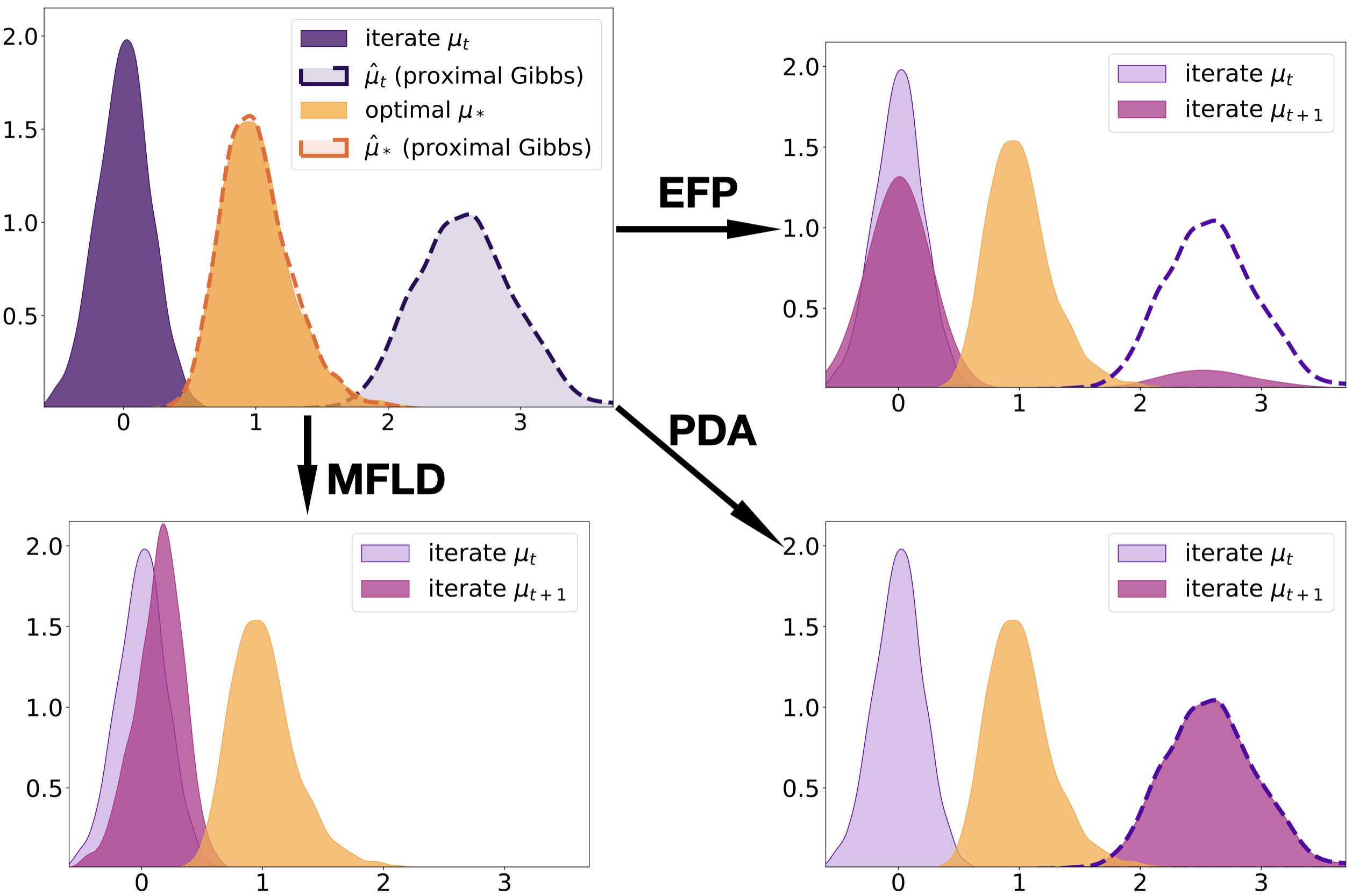
Figure 1: 1D visualization of the parameter distribution of mean-field two-layer neural network (tanh) optimized by the mean-field Langevin dynamics (MFLD), particle dual averaging(PDA), and entropic fictitious play (EFP), all of which can solve the self-consistent equation $\mu=\hat{\mu}$, where $\hat{\mu}$ is the proximal Gibbs measure associated with $\mu$. We set $\lambda=\lambda^{\prime}=10^{-2}$.

An important observation behind the design of these new algorithms is a self-consistent condition of the global optimum (hu2019mean), namely, the optimal solution to the objective (1) must satisfy

$$\mu=\hat{\mu},\quad\text{where~{}}\hat{\mu}(x)\propto\exp\left(-\frac{1}{\lambda}\frac{\delta F(\mu)}{\delta\mu}(x)\right),$$ (2)

in which $\frac{\delta F}{\delta\mu}$ denotes the first-variation of $F$. Following nitanda2022convex, we refer to $\hat{\mu}$ as the proximal Gibbs distribution. Based on properties of $\hat{\mu}$, oko2022psdca and nitanda2022convex established a primal-dual formulation of the optimization problem in the finite-sum setting.

In this work, we analyze a different update rule that optimizes (1) recently proposed in ren2022entropic termed the entropic fictitious play (EFP). The EFP update is inspired by the classical fictitious play in game theory for learning Nash equilibria (brown1951iterative), which has been revisited by cardaliaguet2017learning; hadikhanloo2019finite; perrin2020fictitious; lavigne2022generalized in the context of mean-field games. Intuitively, the EFP method successively accumulates $\hat{\mu}-\mu$ to the current iteration $\mu$ with an appropriate weight, as illustrated in Figure 2. In light of the self-consistent condition (2), this iteration is quite intuitive and natural, as it can be interpreted as a fixed-point iteration on the optimality condition $\mu=\hat{\mu}$.

Despite its simple structure, EFP can be computationally prohibitive if implemented in a naive way. Specifically, for approximately optimizing mean-field models, we typically utilize a finite-particle discretization of the probability distribution. Then, the additive structure of EFP update requires additional particles to be added at each iteration. Therefore, the number of particles linearly increases in proportion to the number of steps, and nontrivial heuristics are needed to reduce the computational costs in general settings.

1.1 Our Contributions

In this paper, we present a concise primal-dual analysis of EFP in the finite-sum setting (e.g., empirical risk minimization). We establish convergence in both continuous- and discrete-time of the primal and dual objectives, which is equivalent to the convergence of the Kullback-Leibler ($\mathrm{KL}$) divergence between $\mu$ and $\hat{\mu}$. Furthermore, our framework naturally suggests an efficient implementation of EFP for finite-sum problems, where the memory consumption remains constant across the iterations. Our contributions can be summarized as follows.

• We provide a simple analysis of EFP for finite-sum problems through the primal-dual framework. Our global convergence result holds in both continuous-and discrete-time settings (Theorem LABEL:theorem:dual-convergence and LABEL:theorem:dual-convergence-discrete).

• Our theory suggests a memory-efficient implementation of EFP (Algorithm 2). Specifically, we do not memorize all particles from the previous iterations, but instead store the information via the proximal Gibbs distribution, with memory cost that only depends on the number of training samples but not the number of iterations.

• We present a connection between EFP and gradient-boosting methods, which enables us to establish discrete-time global convergence based on the Frank-Wolfe argument (Theorem LABEL:theorem:fw-convergence). In other words, in combination with the above algorithmic benefit in the finite-sum setting, EFP can be regarded as a memory-efficient version of the gradient-boosting method.

• We employ our novel implementation of EFP in various experiments including neural network learning and image synthesis (tian2022modern).

1.2 Notations

$\|\cdot\|_{2},~{}\|\cdot\|_{\infty}$ denote the Euclidean norm and uniform norm, respectively. Given a probability distribution $\mu$ on $\mathbb{R}^{d}$, we write the expectation w.r.t. $\theta\sim\mu$ as $\mathbb{E}_{\theta\sim\mu}[\cdot]$ or simply $\mathbb{E}_{\mu}[\cdot]$, $\mathbb{E}[\cdot]$ when the random variable and distribution are obvious from the context; e.g. for a function $f:\mathbb{R}^{d}\rightarrow\mathbb{R}$, we write $\mathbb{E}_{\mu}[f]=\int f(\theta)\mathrm{d}\mu(\theta)$ when $f$ is integrable. $\mathrm{KL}$ stands for the Kullback-Leibler divergence: $\mathrm{KL}(\mu\|\mu^{\prime})\overset{\mathrm{def}}{=}\int\mathrm{d}\mu(\theta)\log\frac{\mathrm{d}\mu}{\mathrm{d}\mu^{\prime}}(\theta)$ and $\mathrm{Ent}$ stands for the negative entropy: $\mathrm{Ent}(\mu)=\int\mathrm{d}\mu(\theta)\log\frac{\mathrm{d}\mu}{\mathrm{d}\theta}(\theta)$. Let $\mathcal{P}_{2}$ be the space of probability distributions on $\mathbb{R}^{d}$ such that absolutely continuous with respect to Lebesgue measure and the entropy and second moment are well-defined.

Preliminaries

2.1 Problem Setup

We say the functional $G:\mathcal{P}_{2}\to\mathbb{R}$ is differentiable and convex when $G$ satisfies the following. First, there exists a functional (referred to as a first variation): $\frac{\delta G}{\delta\mu}:~{}\mathcal{P}_{2}\times\mathbb{R}^{d}\ni(\mu,\theta)\mapsto\frac{\delta G}{\delta\mu}(\mu)(\theta)\in\mathbb{R}$ such that for any $\mu,\mu^{\prime}\in\mathcal{P}_{2}$,

$$\left.\frac{\mathrm{d}G(\mu+\epsilon(\mu^{\prime}-\mu))}{\mathrm{d}\epsilon}\right|_{\epsilon=0}=\int\frac{\delta G}{\delta\mu}(\mu)(\theta)\mathrm{d}(\mu^{\prime}-\mu)(\theta)$$

and $G$ satisfies the convexity condition:

$$G(\mu^{\prime})\geq G(\mu)+\int\frac{\delta G}{\delta\mu}(\mu)(\theta)\mathrm{d}(\mu^{\prime}-\mu)(\theta).$$ (3)

Let $F_{0}:\mathcal{P}_{2}\to\mathbb{R}$ be differentiable and convex, and define $F(\mu)=F_{0}(\mu)+\lambda^{\prime}\mathbb{E}_{\mu}[\|\theta\|_{2}^{2}]$. We consider the minimization of an entropy-regularized convex functional:

$$\min_{\mu\in\mathcal{P}_{2}}\left\{\mathcal{L}(\mu)=F(\mu)+\lambda\mathrm{Ent}(\mu)\right\}.$$ (4)

Note both $F$ and $\mathcal{L}$ are also differentiable convex functionals. Throughout the paper, we make the following regularity assumption on $F_{0}$.

Assumption 1.

We assume the first variation $\frac{\delta F_{0}}{\delta\mu}$ satisfies the Lipschitz continuity and boundedness in the following sense: there exists constant $M>0$ such that for any $\mu,\mu^{\prime}\in\mathcal{P}_{2}$ and for any $\theta,\theta^{\prime}\in\mathbb{R}^{d}$,

$$\left|\frac{\delta F_{0}}{\delta\mu}(\mu)(\theta)-\frac{\delta F_{0}}{\delta\mu}(\mu)(\theta^{\prime})\right| \leq M(W_{2}(\mu,\mu^{\prime})+\|\theta-\theta^{\prime}\|_{2}),$$

$$\left|\frac{\delta F_{0}}{\delta\mu}(\mu)(\theta)\right| \leq M,$$

where $W_{2}$ is the $2$-Wasserstein distance.

For $\mu\in\mathcal{P}_{2}$, we introduce the proximal Gibbs distribution, which plays a key role in our analysis (for basic properties see nitanda2022convex; chizat2022mean).

Definition 1 (Proximal Gibbs distribution).

We define $\hat{\mu}$ be the Gibbs distribution so that

$$\frac{\mathrm{d}\hat{\mu}}{\mathrm{d}\theta}(\theta)=\frac{\exp\left(-\frac{1}{\lambda}\frac{\delta F(\mu)}{\delta\mu}(\theta)\right)}{Z(\mu)},$$ (5)

where $Z(\mu)$ is the normalization constant and $\mathrm{d}\hat{\mu}/\mathrm{d}\theta$ represents the density function w.r.t. Lebesgue measure.

Remark 1.

Under Assumption 1, the existence and uniqueness of the minimizer $\mu_{*}\in\mathcal{P}_{2}$ of $\mathcal{L}$ is guaranteed by ren2022entropic, and $\mu_{*}$ satisfies the first-order optimality condition: $\mu_{*}=\hat{\mu}_{*}$ (hu2019mean).

We focus on the finite-sum setting as follows. Given differentiable convex functions: $\ell_{i}:\mathbb{R}\rightarrow\mathbb{R}$ and functions $h_{i}:\mathbb{R}^{d}\rightarrow\mathbb{R}$ ($i\in\{1,\ldots,n\}$), we consider the following minimization problem:

$$\min_{\mu\in\mathcal{P}_{2}}\left\{\mathcal{L}(\mu)=\frac{1}{n}\sum_{i=1}^{n}\ell_{i}(\mathbb{E}[h_{i}])+\lambda^{\prime}\mathbb{E}[\|\theta\|_{2}^{2}]+\lambda\mathrm{Ent}(\mu)\right\},$$ (6)

where the expectation is taken with respect to $\theta\sim\mu$, i.e., $\mathbb{E}[h_{i}]=\mathbb{E}_{\theta\sim\mu}[h_{i}(\theta)]$. Note that this problem is a special case of (4) by setting $F_{0}(\mu)=\frac{1}{n}\sum_{i=1}^{n}\ell_{i}(\mathbb{E}_{\mu}[h_{i}(\theta)])$.

2.2 Example Applications

One noticeable example of problem (6) is the learning of mean-field neural networks via empirical risk minimization.

Example 1 (Mean-field model).

Let $h(\theta,\cdot):\mathcal{X}\rightarrow\mathbb{R}$ be a function parameterized by $\theta\in\mathbb{R}^{d}$, where $\mathcal{X}$ is the data space. The mean-field model is an integration of $h(\theta,\cdot)$ with respect to the distribution $\mu\in\mathcal{P}_{2}$ over the parameter space: $\mathbb{E}_{\theta\sim\mu}[h(\theta,\cdot)]$. Given training examples $\{(x_{i},y_{i})\}_{i=1}^{n}\subset\mathcal{X}\times\mathbb{R}$, denote $h_{i}(\theta)$ as the output $h(\theta,x_{i})$. Then we may choose the loss term as $\ell_{i}(\mathbb{E}_{\mu}[h_{i}(\theta)])=\ell(y_{i},\mathbb{E}[h(\theta,x_{i})])$, for convex loss functions such as the squared loss $\ell(y,y^{\prime})=0.5(y-y^{\prime})^{2}$ and the logistic loss $\log(1+\exp(-yy^{\prime}))$.

Another example that falls into the framework of (6) is density estimation using a mixture model.

Example 2 (Density Estimation).

Let $\mu*g_{\delta}$ ($\mu\in\mathcal{P}_{2}$) be the Gaussian convolution of $\mu$:

$$\mu*g_{\delta}(\cdot)\propto\int\exp\left(-\frac{\|\theta-\cdot\|_{2}^{2}}{2\sigma^{2}}\right)\mathrm{d}\mu(\theta),$$

where $g_{\delta}(\theta)=(2\pi\sigma^{2})^{-d/2}\exp(-\|\theta^{2}\|/(2\sigma^{2}))$. Let $\{\zeta_{i}\}_{i=1}^{n}\subset\mathbb{R}^{d}$ be the i.i.d. observations. Then, the log-likelihood $-\sum_{i=1}^{n}\log(\mu*g_{\delta}(\zeta_{i}))$ can be written as $\sum_{i=1}^{n}\ell_{i}(\mathbb{E}_{\mu}[h_{i}])$, by setting $\ell_{i}=-\log$ and $h_{i}(\theta)=g_{\delta}(\theta-\zeta_{i})$ since $\mu*g_{\delta}(\zeta_{i})=\mathbb{E}_{\theta\sim\mu}[g_{\delta}(\theta-\zeta_{i})]$.

Entropic Fictitious Play

3.1 The Ideal Update

The entropic fictitious play (EFP) algorithm (ren2022entropic) is the optimization method that minimizes the objective (4). The continuous evolution $\{\mu_{t}\}_{t\geq 0}\subset\mathcal{P}_{2}$ of the EFP is defined as follows: for $\gamma>0$,

$$\frac{\mathrm{d}\mu_{t}}{\mathrm{d}t}=\gamma(\hat{\mu}_{t}-\mu_{t}).$$ (7)

Under Assumption 1, the existence of differentiable density functions that solve (7) is guaranteed.

The time-discretized version of the EFP can be obtained by the explicit Euler’s method. Given a step-size $\eta>0$,

$$\mu_{t+\eta}=(1-\eta\gamma)\mu_{t}+\eta\gamma\hat{\mu}_{t}.$$ (8)

To execute this update, we need to compute the proximal Gibbs distribution $\hat{\mu}_{t}$, which can be accessed via standard sampling algorithms such as Langevin Monte Carlo. This ideal update is summarized in Algorithm 1 below.

Algorithm 1 Discrete-time Entropic Fictitious Play

  Input: $\mu^{(0)},~{}T,~{}\eta,~{}\gamma$

  for $t=0$ to $T-1$ do

     Compute $\hat{\mu}^{(t)}$ via standard sampling algorithms

     Update $\mu^{(t+1)}=(1-\eta\gamma)\mu^{(t)}+\eta\gamma\hat{\mu}^{(t)}$

  end for

  Return $\mu^{(T)}$

As previously remarked, in light of the first-order optimality condition $\mu_{*}=\hat{\mu}_{*}$, the discrete-time EFP (8) is an intuitive update that mirrors the fixed-point iteration methods. However, the naive particle implementation of (8) would be extremely expensive in terms of memory cost. In particular, the additive structure of the discrete-time EFP update requires us to store all the past particles along the trajectory. In other words, the memory cost scales linearly with the number of iterations. This prohibits the practical use of EFP beyond very short time horizon.

3.2 Efficient Particle Update for Finite-sum Settings

We now present an efficient implementation of discrete-time EFP by exploiting the finite-sum structure as in nitanda2020particle; oko2022psdca. For comparison, we first provide a recap for the naive implementation. To execute Algorithm 1, we run a sampling algorithm for each Gibbs distribution $\hat{\mu}^{(t)}$, and build an approximation $\hat{\mu}^{(t)}\sim\frac{1}{m}\sum_{r=1}^{m}\delta_{\theta_{r}^{(t)}}$ by finite particles $\theta_{r}^{(t)}\sim\hat{\mu}^{(t)}~{}(r=1,2,\ldots,m)$, where $\delta_{\theta}$ is the Dirac measure at $\theta\in\mathbb{R}^{d}$. Then, the approximation $\underline{\mu}^{(t+1)}$ to $\mu^{(t+1)}$ can be recursively constructed as follows:

$$\underline{\mu}^{(t+1)}=(1-\eta\gamma)\underline{\mu}^{(t)}+\frac{\eta\gamma}{m}\sum_{r=1}^{m}\delta_{\theta_{r}^{(t)}}.$$ (9)

It is clear that $\underline{\mu}^{(t)}$ consists of all particles obtained up to the $t$-th iteration, and thus the number of particles accumulates linearly with respect to the number of iterations.

Alternative implementation.

Our starting observation is that sampling algorithms for the Gibbs distribution such as Langevin Monte Carlo only require the computation of the gradient of the potential function. Recall that the potential function $\nabla\frac{\delta F(\mu^{(t)})}{\delta\mu}(\theta)$ of the proximal Gibbs distribution $\hat{\mu}^{(t)}$ for finite-sum problems (6) is written as follows:

$$\frac{1}{n}\sum_{i=1}^{n}\ell^{\prime}_{i}(\mathbb{E}_{\mu^{(t)}}[h_{i}(\theta)])\nabla h_{i}(\theta)+2\lambda^{\prime}\theta.$$ (10)

Hence to approximate (10), we do not need to store particles constituting $\underline{\mu}^{(t)}$ themselves, but only the empirical averages: $\mathbb{E}_{\underline{\mu}^{(t)}}[h_{i}(\theta)]$ ($i=1,2,\ldots,n$). Then, we notice that these empirical averages can be recursively computed in an online manner, because of the additive structure of the EFP update (9): for $i=1,2,\ldots,n$,

$$\mathbb{E}_{\underline{\mu}^{(t+1)}}[h_{i}(\theta)]=(1-\eta\gamma)\mathbb{E}_{\underline{\mu}^{(t)}}[h_{i}(\theta)]+\frac{\eta\gamma}{m}\sum_{r=1}^{m}h_{i}(\theta_{r}^{(t)}).$$

It is clear that the number of particles required to compute the above update is $m$ (i.e., the number of samples drawn from the current Gibbs distribution), which can be kept constant during training. This gives a memory-efficient and implementable EFP update, which is described in Algorithm 2 using Langevin Monte Carlo (the sampling algorithm can be replaced by other alternatives). For simplicity, we denote $H^{(t)}_{i}=\mathbb{E}_{\underline{\mu}^{(t)}}[h_{i}(\theta)]$ in the algorithm description.

Algorithm 2 Efficient Implementation of EFP for Finite-sum Problem

  Input: $\mu^{(0)},~{}\lambda,~{}\lambda^{\prime},~{}T,~{}S,~{}m,~{}\eta,~{}\gamma,~{}\eta^{\prime}$

  Randomly sample $m$ particles $\{\theta_{r}^{(-1)}\}_{r=1}^{m}$ from $\mu^{(0)}$

  Compute initial empirical averages: for $i\in\{1,2,\ldots,n\}$

  $H_{i}^{(0)}\leftarrow\frac{1}{m}\sum_{r=1}^{m}h_{i}(\theta_{r}^{(-1)})$

  for $t=0$ to $T-1$ do

     Initialize $\{\overline{\theta}_{r}^{(0)}\}_{r=1}^{m}$ (e.g., $\{\overline{\theta}_{r}\}_{r=1}^{m}\leftarrow\{\theta_{r}^{(t-1)}\}_{r=1}^{m}$)

     for $s=0$ to $S-1$ do

        Run Langevin Monte-Carlo: for $r\in\{1,2,\ldots,m\}$

        $g^{(s)}(\overline{\theta}_{r}^{(s)})\leftarrow\frac{1}{n}\sum_{i=1}^{n}\ell^{\prime}_{i}(H_{i}^{(t)})\nabla h_{i}(\overline{\theta}_{r}^{(s)})$

        $\xi_{r}^{(s)}\sim\mathcal{N}(0,I_{d})$ (i.i.d. Gaussian noise)

        $\overline{\theta}_{r}^{(s+1)}\leftarrow(1-2\eta^{\prime}\lambda^{\prime})\overline{\theta}_{r}^{(s)}-\eta^{\prime}g^{(s)}(\overline{\theta}_{r}^{(s)})+\sqrt{2\eta^{\prime}\lambda}\xi_{r}^{(s)}$

     end for

     $\{\theta_{r}^{(t)}\}_{r=1}^{m}\leftarrow\{\overline{\theta}_{r}^{(S)}\}_{r=1}^{m}$

     Update empirical averages: for $i\in\{1,2,\ldots,n\}$

     $H_{i}^{(t+1)}\leftarrow(1-\eta\gamma)H_{i}^{(t)}+\frac{\eta\gamma}{m}\sum_{r=1}^{m}h_{i}(\theta_{r}^{(t)})$

  end for

  Return $\{\theta_{r}^{(T-1)}\}_{r=1}^{m}$ and $\{H_{i}^{(T)}\}_{i=1}^{n}$