Attribution-Scores and Causal Counterfactuals as Explanations in Artificial Intelligence

Abstract

In this expository article we highlight the relevance of explanations for artificial intelligence, in general, and for the newer developments in explainable AI, referring to origins and connections of and among different approaches. We describe in simple terms, explanations in data management and machine learning that are based on attribution-scores, and counterfactuals as found in the area of causality. We elaborate on the importance of logical reasoning when dealing with counterfactuals, and their use for score computation.

1 Introduction

The search for explanations belongs to human nature, and as a quest, it has been around since the inception of human beings. Explanations, as a subject, have been investigated in Artificial Intelligence (AI) for some decades, and also, and for a much longer time, in other disciplines, such as Philosophy, Logic, Physics, Statistics. Actually, the explicit study of explanations can be traced back to the ancient Greeks, who were already concerned with causes and effects.  Nowadays, a whole area of artificial intelligence (AI) has emerged, that of Explainable AI (XAI). It has become part of an even larger area, Ethical AI, that encompasses other concerns, such as fairness, responsibility, trust, bias (better, lack thereof), etc.

Research done under XAI has become diverse, intensive, extensive, and definitely, effervescent. Accordingly, it is difficult to keep track of: (a) the origins of some popular approaches to explainability; and (b) the new methodologies, and the possible connections, similarities and differences among them.  It is also the case that AI has become of interest for many stakeholders, and most prominently, for people who may be affected by developments in AI and by the use of AI-based systems. It has also become a subject of investigation or discussion for people who do not directly do research, system development or applications inside AI. This has contributed to a certain degree of confusion about what exactly falls under AI, and the role of XAI within AI.

Consistently with these observations, in this work we will revisit, in intuitive and simple terms, some “classic” approaches to explanations that have been introduced and investigated in AI, and have been established in it for some time. We will also discuss newer approaches to explanations that have emerged mainly in the context of Machine Learning (ML), and have become best examples of Explainable AI.  One of our goals is to make clear that explanations have been investigated in AI much before this “new wave” of XAI arrived [52], and that the new methods build (or can be seen as building) upon older approaches.  We also discuss in more detail the place of XAI in AI at large.

Motivated by our own recent research, we describe some approaches to XAI that are based on assigning numerical scores to elements of an input to an AI system, e.g. an ML-classifier, that give an account of their relevance with respect to the outcome obtained from the system for that particular input. Instead of providing all the mathematical and algorithmic background, we use concrete examples to convey the main ideas and issues. Technical details can be found in the provided bibliographic references.

We end this article with a general discussion of the role of reasoning in XAI as it has been traditionally understood in AI. In general, the current approaches do not explicitly appeal to reasoning, nor are they extended with any kind of logical reasoning. We argue in favor of extending these newer approaches with reasoning capabilities, in particular, with counterfactual reasoning, which has to do with exploring, analyzing and comparing, usually hypothetically, different alternative scenarios. This form of reasoning is at the basis of causal explanations, and other areas of computer science.

This is not an exhaustive survey of explanation methods, nor of XAI. Recent surveys that cover XAI can be found, e.g. in [15, 29, 51, 52]. This expository article can be taken as an invitation and a basis for a broader discussion around explanations, and explainable AI; and also as a motivation to explore some subjects in more detail.

2 The Role of Explanations in AI

Explanations are an important part of Artificial Intelligence (AI), and we can clearly identify a couple of fundamental reasons for this:

• Searching for explanations for external phenomena, observed behaviors, etc., and providing them , are important manifestations of human intelligence, and as such, they become natural subjects of investigation in AI.

• AI systems themselves provide results of different kinds, and they require explanations, for humans and AI systems as well.

The former direction has been investigated in AI and more traditional disciplines, as already mentioned above. The second direction is much newer, because AI systems used at large are also much newer. The “older” kind of explanations can be used and adapted for this second purpose, but also some new forms of explanations, that can be more ad hoc for different kinds of AI systems, have been introduced and investigated in the last few years. Let us consider a simple example, for the gist.

Example 1

Consider a client of bank who is applying for loan. The bank will process his/her application by means of an AI system that will decide if the client should be given the loan or not. In order for the application to be computationally processed, the client is represented as an entity describing him/her, say  $\mathbf{e}=\langle\mathsf{john},\mathsf{18},\mathsf{plumber},\mathsf{70K},$ $\mathsf{harlem},\mathsf{10K},\mathsf{basic}\rangle$, that is, a finite record of feature values. The set of features is $\mathcal{F}=\{\mathsf{Name}$, $\mathsf{Age}$, $\mathsf{Activity}$, $\mathsf{Income}$, $\mathsf{Debt}$, $\mathsf{EdLevel}\}$.

The bank uses a classifier, $\mathcal{C}$, that is an AI system that may have been learned on the basis of existing data about loan applications. There are different ways to build such a system. After receiving input $\mathbf{e}$,  $\mathcal{C}$ returns a label, Yes or No (or $0$ or $1$). In this case, it returns No, indicating that the loan request is rejected.  The client (or the bank executive) asks “Why?”, and would like to have an explanation. The issues are: (a) What kind of explanation?  (b) How could it be provided?  (c) From what? $\Box$

These kinds of motivations and applications are typical of Explainable AI (XAI) these days, and of explainable machine learning, in particular. Actually, the whole area has become part of a larger one, usually called Ethical AI, which includes concerns such as transparency, fairness, bias, trust, responsibility, etc., that should be taken into account when the use of AI systems may affect stakeholders. I’s no wonder that these issues are being discussed and investigated in other disciplines, such as Law, Sociology, Philosophy; and others that are more directly affected by the use of AI systems, e.g. Business, Medicine, Health, etc. Some countries have already passed new legislation forcing AI systems affecting users to provide guarantees of an ethical behaviour [16]. Explainability and interpretability of AI systems are part of this picture.

Some claim that ethical AI research is not part of AI, but about AI. The fact that an increasing number of people who work in this area do not do actual AI research, does not make the area less AI. It is part of AI for several reasons, among them: (a) AI systems should be extended with the capability to provide explanations, and the extended systems would become also AI systems; (b) the individual subjects that fall under ethical AI are developed on a scientific and technical basis by AI researchers, who understand, model and implement explanations; (c) as already mentioned, explanation finding and giving are intelligent human activities worth of investigation under AI; (d) explanations become additional resources for AI system building, e.g. one can (automatically) learn from explanations; etc.

3 Some Classical Models of Explanation

In this section, we will briefly introduce and discuss some approaches to explanations that have been proposed and investigated in the context of AI, actually for a few decades by now. Some of them fall in the area of AI called model-based diagnosis [62], in that the explanation process relies on the use of a mathematical model of a system under observation, e.g. a logical or a probabilistic model. We will use a running example to illustrate different approaches.

3.1 Consistency-based diagnosis

If we are confronting a system that is exhibiting an unexpected or abnormal behavior, we want to obtain a diagnosis for this, i.e. some sort of explanation. Diagnoses are obtained from a model of the system, possibly extended with some additional knowledge. In the following, we briefly describe the approach to diagnosis proposed by Ray Reiter [57], usually called consistency-based diagnosis (CBD).

Example 2

Consider the very simple Boolean circuit in Figure 1, with an And-gate, $A$, and an Or-gate, $O$. The input variables are $a,b,c$, the intermediate output variable for $A$ is $x$, and the final, output variable is $d$; all of them taking values $0$ or $1$. The intended meaning of the propositional variable $a$ is “input $a$ is true” (or takes value $1$), etc.

Figure 1: A Boolean circuit

From a conceptual point of view, this could be a binary classifier, for which an input entity $\mathbf{e}$ is represented by a record of binary values for $a,b,c$. The classifier computes the output $d$, which becomes the binary label assigned to $\mathbf{e}$.  Now, assume we observe the following behavior:

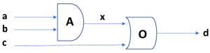
$1\rightarrow$
                           $0\rightarrow$
                           $1\rightarrow$

${\color[rgb]{1,0,0}\longrightarrow 0}$

Figure 2: A malfunctioning Boolean circuit

According to the laws of propositional logic, we should obtain $x=0$ and $d=1$, which is not the case here.  We ask:  Why?  What is wrong?  Or more specifically, What is a diagnosis for the abnormal behavior of the circuit? $\Box$

A more general question now is: What is a diagnosis?  Diagnoses have to be characterized. Since we are adopting a model-based approach, we need a model.  In our example, a logical model of the circuit, when it works properly, is the set of propositional formulas

$$\{(x\longleftrightarrow(a\wedge b)),\ (d\longleftrightarrow(x\vee c))\}.$$ (1)

However, our circuit at hand, by working abnormally, is not modeled by these formulas.

Furthermore, notice that the observation, ${\it Obs}$, represented by the formula:  $a\wedge\neg b\wedge c\wedge\neg d$, indicating that $a$ and $c$ are true, $b$ is false, and $d$ is true, is mutually inconsistent with the ideal model above, that is, there is no assignment of truth values to the propositional variables that makes the combination true. From their combination we cannot logically obtain any useful information, because everything is entailed by an inconsistent set of propositional formulas. We may want instead a model that allows failures, or abnormal behaviors. From such a model, we could try to obtain explanations for those abnormal behaviors.

A better, more flexible model that allows failures, and specifies how components behave under normal conditions is as follows:

$$\mathcal{M}=\{\neg AbA\longrightarrow(x\leftrightarrow(a\wedge b)),\ \ \neg AbO\longrightarrow(d\leftrightarrow(x\vee c))\}.$$ (2)

The first formula says “When $A$ is not abnormal, it works as an And-gate”, etc. Here, ${\it AbA}$ and ${\it AbO}$ are new propositional variables. This is a “weak model of failure” in that it specifies how things behave under normal conditions only, but not under abnormal ones. This is a typical (but non-mandatory) form models take under CBD [22]. The model assumes that the only potentially faulty components are, in this case, the gates (but not the wires connecting them), a modeling choice.   Now gates could be abnormal (or faulty), and $\{{\it Obs}\}\ \cup\ \mathcal{M}$  is a perfectly consistent logical model.

Notice that when one specifies, in addition, that the gates are not abnormal, we have:

$$\{{\it Obs}\}\ \cup\ \mathcal{M}\ \cup\{\neg{\it AbA},\neg{\it AbO}\}\ \mbox{ is \ inconsistent},$$ (3)

as before. So, something has to be abnormal. It is through consistency restoration that we will be able to characterize and compute diagnoses.

Notice that making gate ${\color[rgb]{0,0,1}O}$ abnormal in (3) restores consistency, that is, in contrast to (3),

$${\it Obs}\ \cup\ \mathcal{M}\ \cup\{\neg{\it AbA},\ \underline{{\it AbO}}\}\ \mbox{ is \ consistent}.$$

We are underlying the change we made. More precisely, and by definition, $\{{\it abO}\}$ is a diagnosis.  Similarly, $D^{\prime}=\{{\it abO},{\it abA}\}$ is a diagnosis, because making every gate abnormal also restores consistency:

$${\it Obs}\ \cup\ \mathcal{M}\ \cup\{\underline{{\it AbA}},\ \underline{{\it AbO}}\}\ \mbox{ is \ consistent}.$$

We may consider $D$ as a “better” diagnosis than $D^{\prime}$, because it makes fewer assumptions, is more informative by providing narrower and more focused diagnosis. $D$ is a minimal diagnosis in that it is not set-theoretically included in any other diagnosis. It is also a minimum diagnosis in that it has a minimum cardinality. As expected, different preference criteria could be imposed on diagnosis.

3.2 Abduction

Abduction is a much older approach to obtaining a best explanation for an observation at hand. It can be traced back to Aristotle, and, more recently, to the work by the Philosopher C.S. Peirce [55]. Abductive diagnosis has been extensively investigated in AI, and has become one of the classic approaches to explanations [56, 62, 47].

For the gist, and at the risk of simplifying things too much, a typical example provides the following simple model (a propositional logical theory):  ${\it Covid19}\ \rightarrow\ {\it Breathlessness}$. Now, we observe (for a patient):  ${\it Obs}\!:\ {\it Breathlessness}$. In the light of the only information at hand, that provided by the model, we may “infer” ${\it Covid19}$ as an explanation. However, this is not classical inference in that we are using the implication backwards. So, ${\it Covid19}$ is being abduced from the model and the information (as opposed to classically inferred or deduced), in the sense that:

$$\{\underline{{\it Covid19}}\}\ \cup\ \{{\it Covid19}\ \rightarrow\ {\it Breathlessness}\}\ \models\ {\it Obs},$$ (4)

which defines ${\it Covid19}$ as an abductive explanation.  Here, the symbol $\models$ denotes classical logical consequence.  Of course, if the model becomes more complex, this sort of backward reasoning in search for explanations that support implications (via forward reasoning), becomes much more complex and computationally costly. As expected, one may consider additional preference criteria on abductive explanations, most typically some sort of minimality condition.

Example 3

(example 2 cont.)  Consider the same circuit and observation, in this case ${\it Obs}^{\prime}=\{\neg d\}$, which we would like to entail with additional information provided by abductible facts. We cannot expect to obtain  $\{\underline{{\it abO}}\}\cup\mathcal{M}\ \cup\ \{a\wedge\neg b\wedge c\}\ \models\ \neg d$, with $\mathcal{M}$ as in (2), which is only a weak model of failure.  Actually, the entailment does not hold since $\{{\it abO}\}\cup\mathcal{M}\ \cup\ \{a\wedge\neg b\wedge c\}\ \cup\ \{d\}$ is a consistent theory.

However, if we change the model in order to specify failures, e.g. with  $\mathcal{M}^{\prime}=\{a\wedge b\wedge{\it AbA}\rightarrow\neg x,\ \ x\wedge{\it AbO}\rightarrow\neg d,\ \ c\wedge{\it AbO}\rightarrow\neg d\}$,  we do obtain  $\{\underline{{\it abO}}\}\cup\mathcal{M}^{\prime}\cup\{a,\neg b,c\}\models\neg d$, as expected. It is common, but not mandatory, to use abduction with implicational models [25]. $\Box$

Abduction has found its way into XAI, most prominently, to provide explanations for results from classification models. They are usually called sufficient explanations:  A (hopefully minimal) set of abducible facts that are sufficient to entail the observed label [35, 46, 4].

3.3 Actual causality and responsibility

We can use the running example to illustrate the notion of actual causality [30, 31].

Example 4

(example 2 cont.)  Consider the same circuit as in Figure 2, and the same model as in (2), for which we had in (3):

$$\{a,\neg b,c\}\ \cup\ \mathcal{M}\ \cup\{\neg{\it AbA},\neg{\it AbO}\}\ \cup\ \{\neg d\}\ \mbox{ is inconsistent},$$

which is logically equivalent to:

$$\{a,\neg b,c\}\ \cup\ \mathcal{M}\ \cup\{\neg{\it AbA},\neg{\it AbO}\}\ \models\ d.$$ (5)

In this setting, we will play a counterfactual game consisting in hypothetically changing variables’ truth values, to see if the entailment in (5) changes. Before proceeding, we have to identify the endogenous variables, those on which we have some control, and the exogenous variables we have as a given. This choice is application dependent. In our case, it is natural to consider $a,b,c$ as exogenous, and $x,d,{\it abA},{\it abO}$ as endogenous. Here, the interventions are the hypothetical changes of non-abnormalities into abnormalities, to see if implication in (5) changes as a result. (The interventions are also application dependent.)

Switching $\neg{\it abO}$ into ${\it AbO}$, does invalidate the previous entailment:

$$\{a,\neg b,c\}\ \cup\ \mathcal{M}\ \cup\{\neg{\it AbA},\underline{{\it AbO}}\}\ \not\models\ d.$$

For this reason (and by definition), we say that “${\it abO}$ is a counterfactual cause” (for the observation).

However, when we switch ${\it abA}$:  $\{a,\neg b,c\}\ \cup\ \mathcal{M}\ \cup\{\underline{{\it AbA}},\neg{\it AbO}\}\ \models\ d$. The entailment still holds. Accordingly, ${\color[rgb]{0,0,1}{\it AbA}}$ is not a counterfactual cause. For this candidate, an extra counterfactual change, a so-called contingent change, is necessary:  $\{a,\neg b,c\}\ \cup\ \mathcal{M}\ \cup\{\underline{{\it AbA}},\underline{{\it AbO}}\}\ \not\models\ d.$  Had ${\it abO}$ not been already (and alone) a counterfactual cause, ${\it AbA}$ would have been called (by definition) an actual cause with contingency set $\{abO\}$.  So, ${\it AbA}$ is neither a counterfactual nor an actual cause. $\Box$

Actual causality provides counterfactual explanations to observations. In general terms, they are “components” of a system that are a cause for an observed behavior. Counterfactual causes are actual causes with an empty contingency set. Accordingly, counterfactual causes are strong causes in that they, by themselves, explain the observation. Actual (non-counterfactual) causes are weaker causes, they require the company of other components to explain the observation.

Readers who are more familiar with causality based on structural models [54, 59] may be missing them here. Actually, the diagnosis problems can be cast in those terms too. A purely logical model, as in the previous examples, does not distinguish causal directions, or between causes and effects. They can be better represented by a structural model that takes the form of a (directed) causal network.

Example 5

(example 4 cont.) The following causal network represents our diagnosis example, or better, our possibly faulty circuit.

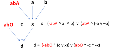
Figure 3: Causal Network

Here, ${\it abA},{\it abO}$ are endogenous variables, which can be subject to counterfactual interventions, which, in this case, amount to making ${\it AbA}$ and ${\it AbO}$ true or false.  Variables $x$ and $d$ are endogenous, and have structural equations associated to them, as shown in Fig. 3, capturing the circuit’s logic. They are unidirectional, so as the edge directions. Contrary to the weak model of failure in (2), the equations specify the behaviour also under abnormality conditions. $\Box$

Actual causality has been extended with the quantitative notion of responsibility [18]. Causes are assigned a numerical score that captures their causal strength. The score takes into account, for endogenous variables, if it is an actual cause or not; and, in the positive case, its contingency sets (CSs).

Example 6

(example 4 cont.)  The responsibility score for an endogenous variable takes into account , in this case, is defined (for the endogenous variables) as follows:

$${\it Resp}({\it abO}) := \frac{1}{1+|\Gamma|}=\frac{1}{1+0}=1,$$

$$\hskip 2.84526pt\mbox{ with $\Gamma$ a minimum-cardinality CS for }{\it abO}.$$

$${\it Resp}({\it abA}) ~{}:=0$$ .

The first case is due to the fact that ${\it abO}$ is a counterfactual cause, and then, has the maximum responsibility, $1$. The second case is due to the fact that ${\it abA}$ is not an actual cause. $\Box$

Actual causality has been applied to provide explanations in the context of relational databases [48, 49, 6]. There, the observation is a query result, and one wants to unveil the causes, inside the database, in the form of, say, database tuples or attribute values in them, for the query to be true (or returning a particular answer). Also, responsibility scores can be assigned to tuples or their attribute values.

Example 7

Consider the relational database instance $D$:

R ⟨c, b ⟩ ⟨a, d ⟩ ⟨b, a⟩       S ⟨a ⟩ ⟨b ⟩ ⟨c ⟩ ⟨d ⟩

The conjunctive query $\mathcal{Q}:\exists x\exists y(S(x)\land R(x,y)\land S(y))$ posed to $D$ is true because join can be satisfied with the database tuples in different ways. For example, the tuples $S(c),R(c,b),S(b)$ jointly satisfy the query condition.

We want to identify tuples as actual causes for the query to be true.  If the tuple $S(b)$ is deleted, the particular instatiation of the join just mentioned above becomes false. However, the query is still true, jointly via the tuples $S(a),R(a,d),$ $S(d)$; or the tuples $S(b),R(b,a),$ $S(a)$. In order to falsify the query, some of these tuples have to be deleted as well. There are different combinations, but a minimum deletion is that of $S(a)$. In more technical terms, in order for $S(b)$ to be an actual cause for the query to be true, it requires a contingency set of tuples to be further deleted. In this case, $\{S(a)\}$ is a minimum-size contingency set, of cardinality $1$. Accordingly, $S(b)$ is an actual cause with causal responsibility ${\it Resp}(S(b))=\frac{1}{1+1}=\frac{1}{2}$. Notice that if we just delete $S(a)$, the query is still true.  A condition on contingency sets for an actual cause is that its deletion alone does not falsify the query; it has to be combined with the cause candidate at hand.

If we, instead, had the following database  $D^{\prime}$  here below,  tuple  $S(b)$  would be a

R ⟨c, b ⟩ ⟨a, d ⟩ ⟨b, b⟩       S ⟨a ⟩ ⟨b ⟩ ⟨c ⟩

counterfactual cause in the sense that it does not require any additional contingent deletion to falsify the query. The empty set is a minimum-size contingency set for it,

and its responsibility becomes $1$, the maximum responsibility.

Tuple $S(c)$ has $\{R(b,b)\}$ as a minimum contingency set, but not $\{S(b)\}$ that alone can falsify the query. We have ${\it Resp}(S(c))=\frac{1}{2}$. $\Box$

The examples above shows similarities between CBD and actual causality, in that in both cases we try to make changes with the purpose of possibly seeing a different outcome.  In fact, a precise connection for the particular case of databases was established in [6], and the connection was appropriately exploited. We give a simple example for the gist.

Example 8

(example 7 cont.) Instead of performing interventions directly on the data-base, and in relation to the query at hand, we can build a CBD problem.

The first observation is that the conjunctive query $\mathcal{Q}\!:\ \exists x\exists y(S(x)\wedge R(x,y)\wedge\ S(y))$ can be transformed into an integrity constraint,  $\kappa\!:\ \neg\exists x\exists y(S(x)\wedge R(x,y)\wedge\ S(y))$, actually a denial constraint that prohibits the satisfaction of the query join (the conjunction).  It holds that $\mathcal{Q}$ is satisfied by $D$ iff $\kappa$ is violated by $D$, which would be considered the faulty behavior.  Accordingly, we specify a system that may not be working as normal, in the sense that the IC can be violated (under abnormal conditions).  The main component of the diagnosis model is the formula:

$$\forall x\forall y(\neg{\it Ab}_{S}(x)\wedge\neg{\it Ab}_{R}(x,y)\wedge\neg{\it Ab}_{S}(y)\ \longrightarrow\ \neg(S(x)\wedge R(x,y)\wedge\ S(y)).$$ (6)

Here, we have introduced one auxiliary abnormality predicate for each database predicate. This formula says that when the tuples are not abnormal, they do not participate in the violation of the IC $\kappa$. In other words, under the normality assumptions, the database behaves as intended (or normal), i.e. satisfying the IC, which in this case, amounts to not making the query true.

For example, the tuples $S(c),R(c,b),S(b)$ in $D$ jointly satisfy the non-negated join on the RHS of (6).  In order to make (6) true, at least one of ${\it Ab}_{S}(c)$, ${\it Ab}_{R}(c,b)$, ${\it Ab}_{R}(b)$ has to be true. The rest continues as with Example 2.  The tuples whose associated abnormality atoms become true are, by definition, the actual causes for the query to be true. $\Box$

In the database context, actual causality was also connected with abductive diagnosis for Datalog queries [7].

4 Attribution Scores in Machine Learning

In machine learning, in situations such as that in Example 1, actual causality and responsibility have been applied to provide counterfactual explanations for classification results, and scores for them. In order to do this, having access to the internal components of the classifier is not needed, but only its input/output relation.

Example 9

(example 1 cont.)  The entity

$$\mathbf{e}\ =\ \langle\mathsf{john},\mathsf{18},\mathsf{plumber},\mathsf{70K},\mathsf{harlem},\mathsf{10K},\mathsf{basic}\rangle$$ (7)

received the label  $1$ from the classifier, indicating that the loan is not granted.  In order to identify counterfactual explanations, we intervene the feature values replacing them by alternative ones from the feature domains, e.g.  $\mathbf{e}_{1}\ =\ \langle\mathsf{john},\underline{\mathsf{25}},\mathsf{plumber},\mathsf{70K},$ $\mathsf{harlem},\mathsf{10K},\mathsf{basic}\rangle$, which receives the label  $0$.  The counterfactual version $\mathbf{e}_{2}=\ \langle\mathsf{john},\mathsf{18},$ $\mathsf{plumber},\underline{\mathsf{80K}},\underline{\mathsf{brooklyn}},\mathsf{10K},\mathsf{basic}\rangle$ also get label  $0$. Assuming, in the latter case, that none of the single changes alone switch the label, we could say that $\mathsf{Age}=\mathsf{25}$, so as $\mathsf{Income}=\mathsf{70K}$ with contingency $\mathsf{Location}=\mathsf{harlem}$ (and the other way around) in $\mathbf{e}$ are (minimal) counterfactual explanations, by being actual causes for the observed label.

We could go one step beyond, and define responsibility scores:  ${\it Resp}(\mathbf{e},\mathsf{Age}):=1$, and ${\it Resp}(\mathbf{e},\mathsf{Income}):=\frac{1}{2}$ (due to the additional, required, contingent change). This choice does reflect the causal strengths of attribute values in $\mathbf{e}$. However, it could be the case that only by changing the value of $\mathsf{Age}$ to $\mathsf{25}$ we manage to switch the label, whereas for all the other possible values for $\mathsf{Age}$ (while nothing else changes), the label is always No. It seems more reasonable to redefine responsibility by considering an average involving all the possible labels obtained in this way. $\Box$

The direct application of the responsibility score, as in [48, 6], works fine for explanation scores when features are binary, say taking values $0$ or $1$, [12, 11]. However, when features have more than two values, it makes sense to extend the definition of the responsibility score.

4.1 The generalized $\mathbf{{\it Resp}}$ score

In [8], a generalized ${\it Resp}$ score was introduced and investigated. We describe it next in intuitive terms, and appealing to Example 9.

1. For an entity $\mathbf{e}$ classified with label $L(\mathbf{e})=1$,  and a feature $F^{\star}$, whose value $F^{\star}(\mathbf{e})$ appears in $\mathbf{e}$, we want a numerical responsibility score ${\it Resp}(\mathbf{e},F^{\star})$, characterizing the causal strength of $F^{\star}(\mathbf{e})$ for outcome $L(\mathbf{e})$.  In the example, $F^{\star}=\mathsf{Salary}$, $F^{\star}(\mathbf{e})=\mathsf{70K}$, and $L(\mathbf{e})=1$.

2. While we keep the original value for $\mathsf{Salary}$ fixed, we start by defining a “local” score for a fixed contingent assignment $\Gamma:=\bar{w}$, with $F^{\star}\notin\Gamma\subseteq\mathcal{F}$.  We define $\mathbf{e}^{\Gamma,\bar{w}}:=\mathbf{e}[\Gamma:=\bar{w}]$, the entity obtained from $\mathbf{e}$ by changing (or redefining) its values for features in $\Gamma$, according to $\bar{w}$.

   In the example, it could be $\Gamma=\{\mathsf{Location}\}$, and $\bar{w}:=\langle\mathsf{brooklin}\rangle$, a contingent (new) value for $\mathsf{Location}$. Then, $\mathbf{e}^{\{\mathsf{Location}\},\langle\mathsf{brooklin}\rangle}=\mathbf{e}[\mathsf{Location}:=\mathsf{brooklin}]=\langle\mathsf{john},\mathsf{25},\mathsf{plumber},\mathsf{70K},$ $\underline{\mathsf{brooklin}},\mathsf{10K},$ $\mathsf{basic}\rangle$.

   We make sure (or assume in the following) that $L(\mathbf{e}^{\Gamma,\bar{w}})=L(\mathbf{e})=1$ holds.  This is because, being these changes only contingent, we do not expect them to switch the label by themselves, but only and until the “main” counterfactual change on $F^{\star}$ is made.

   In the example, we assume $L(\mathbf{e}[\mathsf{Location}:=\mathsf{brooklin}])=1$.  Another case could be $\mathbf{e}^{\Gamma^{\prime}\!,\bar{w}^{\prime}}$​​, with $\Gamma^{\prime}=\{\mathsf{Activity},\mathsf{Education}\}$, and $\bar{w}^{\prime}=\langle\mathsf{accountant},\mathsf{medium}\rangle$, with $L(\mathbf{e}^{\Gamma^{\prime}\!,\bar{w}^{\prime}})=1$.

3. Now, for each of those $\mathbf{e}^{\Gamma,\bar{w}}$ as in the previous item, we consider all the different possible values $v$ for $F^{\star}$, while the values for all the other features are fixed as in $\mathbf{e}^{\Gamma,\bar{w}}$.

   For example, starting from $\mathbf{e}[\mathsf{Location}:=\mathsf{brooklin}]$, we can consider $\mathbf{e}_{1}^{\prime}:=$ $\mathbf{e}[\mathsf{Location}:=\mathsf{brooklin};\underline{\mathsf{Salary}:=\mathsf{60K}}]$  (which is the same as $\mathbf{e}^{\mathsf{Location},\langle\mathsf{brooklin}\rangle}[$ $\mathsf{Salary}$ $:=\mathsf{60K}]$), obtaining, e.g. $L(\mathbf{e}_{1}^{\prime})=1$.  However, for $\mathbf{e}_{2}^{\prime}:=$ $\mathbf{e}[\mathsf{Location}:=\mathsf{brooklin};$ $\underline{\mathsf{Salary:=80}}]$, we now obtain, e.g. $L(\mathbf{e}_{2}^{\prime})=0$, etc.

   For a fixed (potentially) contingent change $(\Gamma,\bar{w})$ on $\mathbf{e}$, we consider the difference between the original label $1$ and the expected label obtained by further modifying the value of $F^{\star}$ (in all possible ways).  This gives us a local responsibility score,   local to $(\Gamma,\bar{w})$:

   $${\it Resp}(\mathbf{e},F^{\star},\underline{\Gamma,\bar{w}}) := \frac{L(\mathbf{e})-\mathbb{E}(~{}L(\mathbf{e}^{\prime})~{}|~{}F(\mathbf{e}^{\prime})=\ F(\mathbf{e}^{\Gamma,\bar{w}}),\ \forall F\in(\mathcal{F}\smallsetminus\{F^{\star}\}~{})}{1+|\Gamma|}$$ (8)

   $$= \frac{1-\mathbb{E}(~{}L(\mathbf{e}^{\Gamma,\bar{w}}[F^{\star}:=v])~{}|~{}v\in{\it Dom}(F^{\star})~{})}{1+|\Gamma|}.$$

   This local score takes into account, so as the original responsibility score in Section 3.3, the size of the contingency set $\Gamma$.

   We are assuming here that there is a probability distribution over the entity population $\mathcal{E}$. It could be known from the start, or it could be an empirical distribution obtained from a sample. As discussed in [8], the choice (or whichever distribution that is available) is relevant for the computation of the general ${\it Resp}$ score, which involves the local ones (coming right here below).

4. Now, generalizing the terms introduced in Section 3.3, we can say that the value $F^{\star}(\mathbf{e})$ is an actual cause for label $1$ when, for some $(\Gamma,\bar{w})$, (8) is positive: at least one change of value for $F^{\star}$ in $\mathbf{e}$ changes the label (with the company of $(\Gamma,\bar{w})$).

   When $\Gamma=\emptyset$ (and then, $\bar{w}$ is an empty assignment), and (8) is positive, it means that at least one change of value for $F^{\star}$ in $\mathbf{e}$ switches the label by itself. As before, we can say that $F^{\star}(\mathbf{e})$ is a counterfactual cause. However, as desired and expected, it is not necessarily the case anymore that counterfactual causes (as original values in $\mathbf{e}$) have all the same causal strength: $F_{i}(\mathbf{e}),F_{j}(\mathbf{e})$ could be both counterfactual causes, but with different values for (8), for example if changes on the first switch the label “fewer times” than those on the second.

5. Now, we can define the global score, by considering the “best” contingencies $(\Gamma,\bar{w})$, which involves requesting from $\Gamma$ to be of minimum size:

   $${\it Resp}(\mathbf{e},F^{\star})\ \ :=\ \max\limits_{{\Gamma,\bar{w}:\ |\Gamma|\ \\ \mbox{\scriptsize\ is min. \& }\mbox{\scriptsize(\ref{eq:star}) $>0$}}}\ {\it Resp}(\mathbf{e},F^{\star},\Gamma,\bar{w}).$$ (9)

   This means that we first find the minimum-size contingency sets $\Gamma$’s for which, for an associated set of value updates $\bar{w}$, (8) becomes greater that $0$. After that, we find the maximum value for (8) over all such pairs $(\Gamma,\bar{w})$. This can be done by starting with $\Gamma=\emptyset$, and iteratively increasing the cardinality of $\Gamma$ by one, until a $(\Gamma,\bar{w})$ is found that makes (8) non-zero. We stop increasing the cardinality, and we just check if there is another $(\Gamma^{\prime},\bar{w}^{\prime})$ that gives a greater value for (8), with $|\Gamma^{\prime}|=|\Gamma|$.  By taking the maximum of the local scores, we have an existential quantification in mind: there must be a good contingency $(\Gamma,\bar{w})$, as long as $\Gamma$ has a minimum cardinality.

With the generalized score, the difference between counterfactual and actual causes is not as relevant as before. In the end, and as discussed under Item 4. above, what matters is the size of the score. Accordingly, we can talk only about “counterfactual explanations with responsibility score $r$”. In Example 9, we could say “$\mathbf{e}_{2}$ is a (minimal) counterfactual for $\mathbf{e}$ (implicitly saying that it switches the label), and the value $\mathsf{60K}$ for $\mathsf{Salary}$ is a counterfactual explanation with responsibility ${\it Resp}(\mathbf{e},\mathsf{Salary})$”. Here, $\mathbf{e}_{2}$ is possibly only one of those counterfactual entities that contribute to making the value for $\mathsf{Salary}$ a counterfactual explanation, and to its (generalized) Resp score.

The generalized ${\it Resp}$ score was applied for different financial data [8], and experimentally compared with a simpler version of responsibility, and with the ${\it Shap}$ score [44], all of which can be applied with a black-box classifier, using only the input/output relation. It was also experimentally compared, with the same data, with a the FICO-score [17] that is defined for and applied to an open-box model, and computes scores by taking into account components of the model, in this case coefficients of nested logistic regressions.

The computation cost of the Resp score is bound to be high in general since, in essence, it explicitly involves in (8) all possible subsets of the set of features; and in (9), also the minimality condition which compares different subsets. Actually, for binary classifiers and in its simple, binary formulation, Resp is already intractable [12].  In [8], in addition to experimental results, there is a technical discussion on the importance of the underlying distribution on the population, and on the need to perform optimized computations and approximations.

4.2 The $\mathbf{{\it Shap}}$ score

The Shap score was introduced in explainable ML in [44], as an application of the general Shapley value of coalition game theory [60], which we briefly describe next.

Consider a set of players $\mathcal{S}$, and a wealth-distribution function (or game function), $\mathcal{G}\!:\mathcal{P}(\mathcal{S})\rightarrow\mathbb{R}$, that maps subsets of $\mathcal{S}$ to real numbers.  The Shapley value of player $p\in\mathcal{S}$ quantifies the contribution of $p$ to the game, for which all different coalitions are considered; each time, with $p$ and without $p$:

$${\it Shapley}(\mathcal{S},\mathcal{G},p):=\sum_{S\subseteq\mathcal{S}\setminus\{p\}}\frac{|S|!(|\mathcal{S}|-|S|-1)!}{|\mathcal{S}|!}(\mathcal{G}(S\cup\{p\})-\mathcal{G}(S)).$$ (10)

Here, $|S|!(|D|-|S|-1)!$ is the number of permutations of $\mathcal{S}$ with all players in $S$ coming first, then $p$, and then all the others.  In other words, this is the expected contribution of $p$ under all possible additions of $p$ to a partial random sequence of players, followed by random sequences of the rest of the players.

The Shapley value emerges as the only quantitative measure that has some specified properties in relation to coalition games [58]. It has been applied in many disciplines.  For each particular application, one has to define a particular and appropriate game function $\mathcal{G}$. Close to home, it has been applied to assign scores to logical formulas to quantify their contribution to the inconsistency of a knowledge base [33], to quantify contributions to the inconsistency of a database [43], and to quantify the contribution of database tuples to making a query true [41, 42].

In different application and with different game functions, the Shapley value turns out to be computationally intractable, more precisely, its time complexity is $\#P$-hard in the size of the input, c.f., for example, [41]. Intuitively, this means that it is at least as hard as any of the problems in the class $\#P$ of problems about counting the solutions to decisions problems (in ${\it NP}$) that ask about the existence of a certain solution [64, 53]. For example, ${\it SAT}$ is the decision problem asking, for a propositional formula, if there exists a truth assignment (a solution) that makes the formula true. Then, $\#\!{\it SAT}$ is the computational problem of counting the number of satisfying assignments of a propositional formula. Clearly, $\#\!{\it SAT}$ is at least as hard as ${\it SAT}$ (it is good enough to count the number of solutions to know if the formula is satisfiable), and ${\it SAT}$ is the prototypical ${\it NP}$-complete problem, and furthermore, $\#\!{\it SAT}$ is $\#P$-hard, actually, $\#\!P$-complete since it belongs to $\#P$. As a consequence, computing the Shapley value can be at least as hard as computing the number of solutions for ${\it SAT}$; a clear indication of its high computational complexity.

As mentioned earlier in this section, the Shap score is a particular case of the Shapley value in (10). In this case, the players are the features $F$ in $\mathcal{F}$, or, more precisely, the values $F(\mathbf{e})$ they take for a particular entity $\mathbf{e}$, for which we have a binary classification label, $L(\mathbf{e})$, we want to explain. The explanation comes in the form of a numerical score for $F(\mathbf{e})$, reflecting its relevance for the observed label. Since all the feature values contribute to the resulting label, we may conceive the features values as players in a coalition game.

The game function, for a given subset $S$ of the features, is the expected (value of the) label over all possible entities whose values coincide with those of $\mathbf{e}$ for the features in $S$:

$$\mathcal{G}_{\mathbf{e}}(S):=\mathbb{E}(L(\mathbf{e^{\prime}})~{}|~{}\mathbf{e}^{\prime}\in\mathcal{E}\ \mbox{ and }\ \mathbf{e}^{\prime}_{\!S}=\mathbf{e}_{S}),$$ (11)

where $\mathbf{e}^{\prime}_{S},\mathbf{e}_{S}$ denote the projections of $\mathbf{e}^{\prime}$ and $\mathbf{e}$ on $S$, resulting in two subrecords of feature values.  We can see that the game function depends on the entity at hand $\mathbf{e}$.

With the game function in (10), we obtain the Shap score for a feature value $F^{\star}(\mathbf{e})$ in $\mathbf{e}$:

$${\it Shap}(\mathcal{F},\mathcal{G}_{\mathbf{e}},F^{\star}) := \!\!\!\!\!\sum_{S\subseteq\mathcal{F}\setminus\{F^{\star}\}}\frac{|S|!(|\mathcal{F}|-|S|-1)!}{|\mathcal{F}|!}[\mathbb{E}(L(\mathbf{e}^{\prime}|\mathbf{e}^{\prime}_{S\cup\{F^{\star}\}}=\mathbf{e}_{S\cup\{F^{\star}\}})-$$ (12)

$$\hskip 120.92421pt\mathbb{E}(L(\mathbf{e}^{\prime})|\mathbf{e}^{\prime}_{S}=\mathbf{e}_{S})].$$

Example 10

(example 9 cont.)  For the fixed entity $\mathbf{e}$ in (7) and feature $F^{\star}=\mathsf{Salary}$, one of the terms in (12) is obtained by considering $S=\{\mathsf{Location}\}\subseteq\mathcal{F}$:

$$\frac{|1|!(7-1-1)!}{7!}\times(\mathcal{G}_{\mathbf{e}}(\{\mathsf{Location}\}\cup\{\mathsf{Salary}\})-\mathcal{G}_{\mathbf{e}}(\{\mathsf{Location}\}))$$

$$\hskip 99.58464pt=\ \frac{1}{42}\times(\mathcal{G}_{\mathbf{e}}(\{\mathsf{Location},\mathsf{Salary}\})-\mathcal{G}_{\mathbf{e}}(\{\mathsf{Location}\})),$$

with, e.g.,  $\mathcal{G}_{\mathbf{e}}(\{\mathsf{Location},\mathsf{Salary}\})=\mathbb{E}(L(\mathbf{e}^{\prime})~{}|~{}\mathbf{e}^{\prime}\in\mathcal{E},\ \mathsf{Location}(\mathbf{e}^{\prime})=\mathsf{harlem},\mbox{ and }$ $\mathsf{Salary}(\mathbf{e}^{\prime})=\mathsf{70K})$,   that is, the expected label over all entities that have the same values as $\mathbf{e}$ for features $\mathsf{Salary}$ and $\mathsf{Location}$.  Then,  $\mathcal{G}_{\mathbf{e}}(\{\mathsf{Location},\mathsf{Salary}\})-\mathcal{G}_{\mathbf{e}}(\{\mathsf{Location}\})$ is the expected difference in the label between the case where the values for $\mathsf{Location}$ and $\mathsf{Salary}$ are fixed as for $\mathbf{e}$, and the case where only the value for $\mathsf{Location}$ is fixed as in $\mathbf{e}$, measuring a local contribution of $\mathbf{e}$’s value for $\mathsf{Salary}$. After that, all these local differences are averaged over all subsets $S$ of $\mathcal{F}$, and the permutations in which they participate. $\Box$

We can see that, so as the Resp score, Shap is a local explanation score, for a particular entity at hand $\mathbf{e}$.  Since the introduction of Shap in this form, some variations have been proposed. So as for Resp, Shap depends, via the game function, on an underlying probability distribution on the entity population $\mathcal{E}$. The distribution may impact not only the Shap scores, but also their computation [8].

4.3 Computation of the $\mathbf{{\it Shap}}$ score

Boolean classifiers, i.e. propositional formulas with binary input features and binary labels, are particularly relevant, per se and because they can represent other classifiers by means of appropriate encodings. For example, the circuit in Figure 1 can be seen as a binary classifier that can be represented, on the basis of (1), by means of the single propositional formula  $((a\wedge b)\vee c)$  that, depending on the binary values for $a,b,c$, also returns a binary value.

Boolean classifiers, as logical formulas, have been extensively investigated. In particular, much is known about the satisfiability problem of propositional formulas, ${\it SAT}$, and also about the model counting problem, i.e. that of counting the number of satisfying assignments, denoted $\#\!{\it SAT}$.  In the area of knowledge compilation, the complexity of $\#\!{\it SAT}$ and other problems in relation to the syntactic form of the Boolean formulas have been investigated [19, 20, 28].  Boolean classifiers turn out to be quite relevant to understand and investigate the complexity of Shap computation.

The computation of Shap is bound to be expensive, for similar reasons as for Resp. For the computation of both, all we need is the input/output relation of the classifier, to compute labels for different alternative entities (counterfactuals). However, in principle, far too many combinations have to go through the classifier. Actually, under the product probability distribution on $\mathcal{E}$ (which assigns independent probabilities to the feature values), even with an explicit, open classifier for binary entities, the computation of Shap can be intractable.

In fact, as shown in [8], for Boolean classifiers in the class ${\it Monotone}2{\it CNF}$, of negation-free propositional formulas in conjunctive normal form with at most two atoms per clause, Shap can be $\#\!P$-hard. This is obtained via a polynomial reduction from $\#{\it Monotone}2{\it CNF}$, the problem of counting the number of satisfying assignments for a formula in the class, which is known to be $\#\!P$-complete [64].  For example, if the classifier is  $(x_{1}\vee x_{2})\wedge(x_{2}\vee x_{3})$, which belongs to $\#{\it Monotone}2{\it CNF}$, the entity $\mathbf{e}_{1}=\langle 1,0,1\rangle$ (with values for $x_{1},x_{2},x_{3}$, in this order) gets label $1$, whereas the entity $\mathbf{e}_{2}=\langle 1,0,0\rangle$ gets label $0$.  The number of satisfying truth assignments, equivalently, the number of entities that get label $1$, is $5$, corresponding to $\langle 1,1,1\rangle$, $\langle 1,0,1\rangle$, $\langle 0,1,1\rangle$, $\langle 0,1,0\rangle$, and $\langle 1,1,0\rangle$.

Given that Shap can be $\#P$-hard, a natural question is whether for some classes of open-box classifiers one can compute Shap in polynomial time in the size of the model and input. The idea is to try to take advantage of the internal stricture and components of the classifier -as opposed to only the input/output relation of the classifier- in order to compute Shap efficiently. We recall from results mentioned earlier in this section that having an open-box model does not guarantee tractability of Shap. Natural classifiers that have been considered in relation to a possible tractable computation of Shap are decision trees and random forests [45].

The problem of tractability of Shap was investigated in detail in [2], and through other methods also in [65]. They briefly describe the former approach in the rest of this section. Tractable and intractable cases were identified, with algorithms for the tractable cases. (Approximations for the intractable cases were further investigated in [3].) In particular, the tractability for decision trees and random forests was established, which required first identifying the right abstraction that allows for a general proof, leaves aside contingent details, and is also broad enough to include interesting classes of classifiers.

In [2], it was proved that, for a Boolean classifier $L$ (identified with its label, the output gate or variable), the uniform distribution on $\mathcal{E}$, and $\mathcal{F}=\{F_{1},\ldots,F_{n}\}$:

$$\#\!{\it SAT}(L)\ =\ 2^{|\mathcal{F}|}\times(L(\mathbf{e})-\sum_{i=1}^{n}{\it Shap}(\mathcal{F},G_{\mathbf{e}},F_{i})).$$ (13)

This result makes, under the usual complexity-theoretic assumptions, impossible for Shap to be tractable for any circuit $L$ for which $\#\!{\it SAT}$ is intractable. (If we could compute Shap fast, we could also compute $\#\!{\it SAT}$ fast, assuming we have an efficient classifier.)  This excludes, as seen earlier in this section, classifiers that are in the class ${\it Monotone}2{\it CNF}$. Accordingly, only classifiers in a more amenable class became candidates, with the restriction that the class should be able to accommodate interesting classifiers. That is how the class of deterministic and decomposable Boolean circuits (dDBCs) became the target of investigation.

Each $\vee$-gate of a dDBC can have only one of the disjuncts true (determinism), and for each $\wedge$-gate, the conjuncts do not share variables (decomposition). Nodes are labeled with $\vee,\wedge$, or $\neg$ gates, and input gates with features (propositional variables) or binary constants. An example of such a classifier, borrowed from [2], is shown in Figure 4, which has four (input) features, and an a gate that returns the output label (the $\wedge$ at the top).  For a counterexample, the BC $((a\wedge b)\vee c)$ for Figure 1 is decomposable, but not deterministic.

Figure 4: A decomposable and deterministic Boolean classifier

Model counting is known to be tractable for dDBCs. However, this does not imply (via (13) or any other obvious way) that Shap is tractable. It is also the case that relaxing any of the determinism or decomposibility conditions makes model counting $\#P$-hard [3], preventing Shap from being tractable.

It turns out that ${\it Shap}$ computation is tractable for dDBCs (under the uniform or the product distribution), from which we also get tractability of ${\it Shap}$ for free for a vast collection of classifiers that can be efficiently compiled into (or represented as) dDBCs; among them we find:  Decision Trees (even with non-binary features), Random Forests, Ordered Binary Decision Diagrams (OBDDs) [14], Deterministic-Decomposable Negation Normal-Forms (dDNNFs), Binary Neural Networks (e.g. via OBDDs) [61], etc.

For the gist, consider the binary decision tree (DT) on the LHS of Figure 5. It can be inductively and efficiently compiled into a dDBC [3, appendix A]. The leaves of the DT become labeled with propositional constants, $0$ or $1$. Each node, $n$, is compiled into a circuit $c(n)$, and the final dDBC corresponds to the compilation, $c(r)$, of the root node $r$, in this case, $c(n7)$ for node $c7$.  Figure 5 shows on the RHS, the compilation $c(n5)$ of node $n5$ of the DT.  If the decision tree is not binary, it is first binarized, and then compiled [3, sec. 7].

               

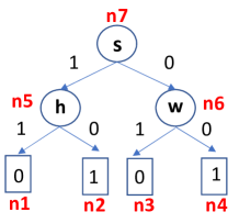
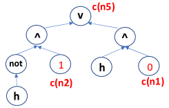
Figure 5: A decision tree and part of its compilation into an dDBC

Abductive explanations have for dDNNF-Boolean circuits have been investigated in [34].

5 Counterfactual Reasoning

As we saw in the preceding sections, counterfactuals are at the basis of the responsibility score. It is captured in (8) that some counterfactual interventions may not change the label of a feature value. However, for a feature value to have a non-zero responsibility, there must be at least one counterfactual intervention on that value that changes the label. In the case of Shap, all counterfactuals are implicit and taken into account in its computation.

Independently from their participation in the definition and computation of attribution scores, counterfactuals are relevant and informative per se [66]. Assuming they satisfy some minimality condition, they tell us what change of feature values may change the label, pointing to the relevance of the original values for the label at hand. Furthermore, in many situations we would like to know what we could do in order to change the label, e.g. granting a loan instead of rejecting it. If those changes can be usefully made in practice, we are talking about actionable counterfactuals, or counterfactuals that are resources [63, 36, 37, 66]. In the ongoing example, changing the age, and then waiting for seven years to get the loan, may not be feasible. Nor changing the name of the applicant from $\mathsf{john}$ to $\mathsf{elon}$. However, slightly increasing the salary might be doable.   We may also want to compare two alternative counterfactuals, or ask about the existence of one with a particular property, e.g. a particular value for a feature, etc.

Working with and analyzing counterfactuals can be made easier and more understandable if we can reason about them under a single platform that includes (or interacts with) the classifier, and the score computation mechanisms, for a particular application. By reasoning we mean, among other tasks, the logical specification of counterfactuals, the entailment of counterfactuals, their analysis, and obtaining them and their properties. Counterfactual reasoning has been investigated from a logical point of view [23].  If we want to put counterfactual reasoning in practice, we need the right logics and their implementations.

We have recently argued in favor of using answer-set programming (ASP) for this task [10]. ASP is a form of logic programming that has several advantages for the kind of problems we are confronting [13], among them: (a) It has the right-expressive power and computational complexity since it can be applied to solve complex combinatorial problems. (b) Through its non-monotonic negation, and associated predicate minimality, it allows to represent the (common sense) inertia or persistence of objects and their properties unless they are explicitly changed (intervened in our case). (c) Logical disjunction allows to specify several alternative counterfactual candidates at once. (d) One can pose queries to obtain results from reasoning (c.f. below). (e) Its possible worlds semantics for the specification leads to multiple models corresponding to equally multiple counterfactuals, with different properties. (f) A cautious and a brave query answering semantics that allow asking what is true in all or in some models, respectively. (g) There are implementations of ASP that can interact with external classifiers.

In essence, one can specify the underlying logical setting, e.g. some classes of classifiers, the possible interventions that lead to counterfactuals, properties such as actionability and other properties that may force counterfactuals “to make sense”, minimality conditions on counterfactuals, and the computation of (some) attribution-scores that are based on counterfactuals. ASPs also allow for score aggregations, for more global and higher-level explanations.

We have used ASP, in particular the DLV system and its various extensions [40], to specify counterfactuals for causality in data management [9] and for explanations in ML [11, 12], including the computation of the simple responsibility score.  However, if we want to compute scores that are defined in terms of of expected values, e.g. Resp or Shap, over probability distributions other than easily specifiable and computable ones, it may be necessary to resort to probabilistic extensions of ASP [5, 38, 39, 32].

Counterfactual reasoning on the basis of ASPs is best seen as query-driven. One can pose all kinds of queries about counterfactuals, for which having a cautious and a brave semantics comes handy. Typical queries request counterfactual with a particular property, e.g. that changes, or does not change a particular feature value; or counterfactuals that exhibit (or avoid) a particular combination of feature values; or pairs of counterfactuals that differ in a pre-specified manner. Queries may ask if a particular feature value is never changed in a (preferred kind of) counterfactual; or about the existence of good counterfactuals that do not change more than a certain number of feature values; or whether there are “similar” counterfactuals with different labels (according to a specified notion of similarity), etc.  C.f. [10, 11, 12] for concrete examples. One can also compare counterfactual entities with pre-specified reference entities for obtaining contrastive explanations [37, 50].

Specifying actionable counterfactuals is only one way to convey relevant application domain knowledge into the definition of counterfactuals. A logical specification allows for much more than that, including the adoption of a domain semantics. We started this section recalling that, in principle, all counterfactuals are considered for the computation of attribution scores. However, it would be much more natural, useful, and possibly also more efficient, to consider and compute counterfactuals that conform to the domain semantics, which can be specified through logical rules and constraints, in such a way that only those are brought into a score computation [12]. For example, since the age of an individual (represented as an entity) never decreases, changing it by a lower value may not make much sense in most applications. Similarly, some combinations of values may not make sense, e.g. $\mathsf{Age}=\mathsf{6}$  and  $\mathsf{MaritalStatus}=\mathsf{married}$.

Considering that counterfactuals are at the very basis of causality, it is not surprising to see that they are playing a prominent role in Explainable AI. However, they have also found applications in Fairness in AI. C.f. [59] and references therein.

Acknowledgements:  Part of this work was funded by ANID - Millennium Science Initiative Program - Code ICN17002.  The author is a Professor Emeritus at Carleton University, Ottawa, Canada; and a Senior Universidad Adolfo Ibáñez (UAI) Fellow, Chile.  Comments by Paloma Bertossi on an earlier version of the article are much appreciated.

References

- [1] Antoine Amarilli,, A., Capelli, F., Monet1, M. and Senellart, P. Connecting Knowledge Compilation Classes Width Parameters. Theory of Computing Systems, 2020, 64:861–914.
- [2] Arenas, M., Barcelo, P., Bertossi, L. and Monet, M. The Tractability of SHAP-scores over Deterministic and Decomposable Boolean Circuits. Proc. AAAI, 2021.
- [3] Arenas, M., Barcelo, P., Bertossi, L. and Monet, M. The Tractability of SHAP-scores over Deterministic and Decomposable Boolean Circuits. Extended version of AAAI 2021 paper. arXiv 2104.08015, 2021.
- [4] Arenas, M., Pablo Barcelo, P., Romero, M. and Subercaseaux, B. On Computing Probabilistic Explanations for Decision Trees. Proc. NeurIPS, 2022.
- [5] Baral, C., Gelfond, M. and Rushton, N. Probabilistic Reasoning with Answer Sets. Theory and Practice of Logic Programming, 2009, 9(1):57-144.
- [6] Bertossi, L. and Salimi, B. From Causes for Database Queries to Repairs and Model-Based Diagnosis and Back. Theory of Computing Systems, 2017, 61(1):191-232.
- [7] Bertossi, L. and Salimi, B. Causes for Query Answers from Databases: Datalog Abduction, View-Updates, and Integrity Constraints. Int. J. Approximate Reasoning, 2017, 90:226-252.
- [8] Bertossi, L., J. Li, J., Schleich, M., Suciu, D. and Vagena, Z. Causality-based Explanation of Classification Outcomes. Proc. 4th International Workshop on “Data Management for End-to-End Machine Learning” (DEEM) at ACM SIGMOD/PODS, 2020, pp. 6:1-10.
- [9] Bertossi, L. Specifying and Computing Causes for Query Answers in Databases via Database Repairs and Repair Programs. Knowledge and Information Systems, 2021, 63(1):199-231.
- [10] Bertossi, L. Score-Based Explanations in Data Management and Machine Learning: An Answer-Set Programming Approach to Counterfactual Analysis. In Reasoning Web. Declarative Artificial Intelligence. Reasoning Web 2021. Springer LNCS 13100, 2022, pp. 145-184.
- [11] Bertossi¡ L. and Reyes, G. Answer-Set Programs for Reasoning about Counterfactual Interventions and Responsibility Scores for Classification. In Proc. 1st International Joint Conference on Learning and Reasoning (IJCLR’21), Springer LNAI 13191, 2022, pp. 41-56.
- [12] Bertossi, L. Declarative Approaches to Counterfactual Explanations for Classification. Theory and Practice of Logic Programming. https://doi.org/10.1017/S1471068421000582. arXiv 2011.07423, 2020.
- [13] Brewka, G., Eiter, T. and Truszczynski, M. Answer Set Programming at a Glance. Communications of the ACM, 2011, 54(12):92-103.
- [14] Bryant, R. E. Graph-Based Algorithms for Boolean Function Manipulation. IEEE Tran. Com., C-35:677–691, 1986.
- [15] Burkart, N. and Huber, M. F. A Survey on the Explainability of Supervised Machine Learning. Journal of Artificial Intelligence Research, 2021, 70:245-317.
- [16] Chatila1, R., Dignum, V., Fisher, M., Giannotti, F., Morik, K., Russell, S. and Yeung, K. Trustworthy AI. In Reflections on Artificial Intelligence for Humanity, 2021, Springer LNAI 12600, pp. 13–39.
- [17] Chen, C., Lin, K., Rudin, C., Shaposhnik, Y., Wang, S. and Wang, T. An Interpretable Model with Globally Consistent Explanations for Credit Risk. arXiv 1811.12615, 2018.
- [18] Chockler, H. and Halpern, J. Y. Responsibility and Blame: A Structural-Model Approach. Journal of Artificial Intelligence Research, 2004, 22:93-115.
- [19] Darwiche, A. and Marquis, P. A Knowledge Compilation Map. Journal of Artificial Intelligence Research, 2002, 17:229–264.
- [20] Darwiche, A. On the Tractable Counting of Theory Models and its Application to Truth Maintenance and Belief Revision. Journal of Applied Non-Classical Logics, 2011, 11(1-2):11-34.
- [21] de Kleer, J., Mackworth, A. and Reiter, R. Characterizing Diagnoses and Systems. Artificial Intelligence, 1992, 56(2-3):197-222.
- [22] de Kleer, J., Mackworth, A. and Reiter, R. Characterizing Diagnoses and Systems. Artificial Intelligence, 1992, 56(2-3):197-222.
- [23] Eiter, T. and Gottlob, G. On the Complexity of Propositional Knowledge Base Revision, Updates, and Counterfactuals. Artificial Intelligence, 1992, 57(2-3):227-270.
- [24] Eiter, T. and Gottlob, G. The Complexity of Logic-Based Abduction. J. ACM, 1995, 42(1): 3-42.
- [25] Eiter, T., Gottlob, G., Leone, N. Abduction from Logic Programs: Semantics and Complexity. Theor. Comput. Sci., 1997, 189(1-2): 129-177.
- [26] Eiter, T., Faber, W., Leone, N. and Pfeifer, G. The Diagnosis Frontend of the DLV System. AI Commununications, 1999, 12(1-2):99-111. Extended version as Tech. Report DBAI-TR-98-20, TU Vienna, 1998.
- [27] Ferrara, A., Pan, G. and Vardi, M. Treewidth in Verification: Local vs. Global. Proc. LPAR 2005, Springer LNAI 3835, 2005, pp. 489–503.
- [28] Gomes, C. P., Sabharwal, A. and Selman, B. Model Counting. Handbook of Satisfiability. IOS Press, 2009, pp. 993-1014.
- [29] Guidotti, R., Monreale, A., Ruggieri, S., Turini, F., Giannotti, F. and Pedreschi, D. A Survey of Methods for Explaining Black Box Models. ACM Comput. Surv., 51(5):1-93.
- [30] Halpern, J. and Pearl, J. Causes and Explanations: A Structural-Model Approach. Part I: Causes. The British Journal for the Philosophy of Science, 2005, 56(4):843-887.
- [31] Halpern, J. Actual Causality. MIT Press, 2016.
- [32] Hahn, S., Janhunen, T., Kaminski, R., Romero, J., Rühling, N. and Schaub, T. Plingo: A System for Probabilistic Reasoning in Clingo Based on LP MLN . Proc. RuleML+RR, 2022, pp. 54-62.
- [33] Hunter A. and Konieczny, S. On the Measure of Conflicts: Shapley Inconsistency Values. Artificial Intelligence, 2010, 174(14):1007–1026.
- [34] Huang, X., Izza, Y., Ignatiev, A., Cooper, M. C., Asher, N. and Marques-Silva, J. Tractable Explanations for d-DNNF Classifiers. Proc. AAAI, 2022, pp. 5719-5728.
- [35] Ignatiev, A., Narodytska, N. and Marques-Silva, J. Abduction-Based Explanations for Machine Learning Models. Proc. AAAI, 2019, pp. 1511-1519.
- [36] Karimi, A-H., von Kügelgen, B. J., Schölkopf, B. and Valera, I. Algorithmic Recourse under Imperfect Causal Knowledge: A Probabilistic Approach. Proc. NeurIPS, 2020.
- [37] Karimi, A.-H., Barthe, G., Schölkopf, B. and Valera, I. A Survey of Algorithmic Recourse: Contrastive Explanations and Consequential Recommendations. ACM Comput. Surv., 2023, 55(5):95:1-95:29. 2022.
- [38] Lee, J. and Yang, Z. LPMLN, Weak Constraints, and P-log. Proc. AAAI, 2017, pp. 1170-1177.
- [39] Lee, J. and Yang, Z. Statistical Relational Extension of Answer Set Programming. This volume, 2023.
- [40] Leone, N., Pfeifer, G., Faber, W., Eiter, T., Gottlob, G., Perri, S. and Scarcello, F. The DLV System for Knowledge Representation and Reasoning. ACM Transactions on Computational Logic, 2006, 7(3):499-562.
- [41] Livshits, E., Bertossi, L., Kimelfeld, B. and Sebag, M. Query Games in Databases”. ACM Sigmod Record, 2021, 50(1):78-85.
- [42] Livshits, E., Bertossi, L., Kimelfeld, B. and Sebag, M. The Shapley Value of Tuples in Query Answering. Log. Methods Comput. Sci., 2021, 17(3).
- [43] Livshits, E. and Kimelfeld, E. The Shapley Value of Inconsistency Measures for Functional Dependencies. Log. Methods Comput. Sci., 2022, 18(2).
- [44] Lundberg, S. and Lee, S.-I. A Unified Approach to Interpreting Model Predictions. Proc. NIPS, 2017, pp. 4765-4774.
- [45] Lundberg, S. M., Erion, G., Chen, H., DeGrave, A., Prutkin, J., Nair, B., Katz, R., Himmelfarb, J., Bansal, N. and Lee, S-I. From Local Explanations to Global Understanding with Explainable AI for Trees. Nature Machine Intelligence, 2020, 2(1):56-67.
- [46] Marques-Silva, J. Logic-Based Explainability in Machine Learning. This volume, 2023.
- [47] Marquis, P. Extending Abduction from Propositional to First-Order Logic. In Fundamentals of Artificial Intelligence Research, 1991, Springer LNAI 535, pp. 141–155.
- [48] Meliou, A., Gatterbauer, W., Moore, K. F. and Suciu, D. The Complexity of Causality and Responsibility for Query Answers and Non-Answers. Proc. VLDB, 2010, pp. 34-41.
- [49] Meliou, A., Gatterbauer, W., Halpern, J.Y., Koch, C., Moore, K. F. and Suciu, D. Causality in Databases. IEEE Data Eng. Bull., 2010, 33(3):59-67.
- [50] Miller, T. Contrastive Explanation: A Structural-Model Approach. The Knowledge Engineering Review, 2021, 36(4):1-24.
- [51] Minh, D., Xiang-Wang, H., Fen-Li, Y. and Nguyen, T. N. Explainable Artificial Intelligence: A Comprehensive Review. Artificial Intelligence Review, 2022, 55:3503–3568.
- [52] Molnar, C. Interpretable Machine Learning: A Guide for Making Black Box Models Explainable, 2020. https://christophm.github.io/interpretable-ml-book
- [53] Papadimitriou, P. Computational Complexity. Addison-Wesley, 1994.
- [54] Pearl, J. Causality: Models, Reasoning and Inference. Cambridge University Press, 2nd Ed., 2009.
- [55] Peirce, C. S. Collected Papers of Charles Sanders Peirce, Vol. 2. Hartsthorne, C. and Weiss, P. (eds.), 1931, Harvard University Press.
- [56] Poole, D. and Mackworth, A. K. Artificial Intelligence. Section 5.7. Cambridge Univ. Press, 2nd Ed., 2017.
- [57] Reiter, R. A Theory of Diagnosis from First Principles. Artificial Intelligence, 1987, 32(1):57-95.
- [58] Roth, A. E. The Shapley Value: Essays in Honor of Lloyd S. Shapley. Cambridge Univ. Press, 1988.
- [59] Roy, S. and Salimi, B. Causal Inference in Data Analysis with Applications to Fairness and Explanations. This volume, 2023.
- [60] Shapley, L. S. A Value for n-Person Games. Contributions to the Theory of Games, 1953, 2(28):307–317.
- [61] Shi, W., Shih, A., Darwiche, A. and Choi, A. On Tractable Representations of Binary Neural Networks. Proc. KR, 2020, pp. 882-892.
- [62] Struss, P. Model-Based Problem Solving. In Handbook of Knowledge Representation, Chap. 4. Elsevier, 2008, pp. 395-465.
- [63] Ustun, B., Spangher, A. and and Liu, Y. Actionable Recourse in Linear Classification. Proc. FAT, 2019, pp. 10–19.
- [64] Valiant, L G. The Complexity Of Enumeration And Reliability Problems. Siam J. Comput., 1979, 8(3):410-421.
- [65] Van den Broeck, G., Lykov, A., Schleich, M. and Suciu, D. On the Tractability of SHAP Explanations. Proc. AAAI, 2021, pp. 6505-6513.
- [66] Verma, S., Boonsanong, V., Hoang, M., Keegan, E., Hines, K. E., Dickerson, J. P. and Shah, C. Counterfactual Explanations and Algorithmic Recourses for Machine Learning: A Review. arXiv 2010.10596, 2022.