Abstract

This paper develops estimation and inference methods for censored quantile regression models with high-dimensional controls. The methods are based on the application of double/debiased machine learning (DML) framework to the censored quantile regression estimator of Buchinsky and Hahn (1998). I provide valid inference for low-dimensional parameters of interest in the presence of high-dimensional nuisance parameters when implementing machine learning estimators. The proposed estimator is shown to be consistent and asymptotically normal. The performance of the estimator with high-dimensional controls is illustrated with numerical simulation and an empirical application that examines the effect of 401(k) eligibility on savings.

Keywords: Double/debiased machine learning, Neyman orthogonality, post-selection inference, high-dimensional data, causal inference, censored quantile regression

Censored Quantile Regression with Many Controls

Seoyun Hong

March 5, 2023

1 Introduction

Censoring is a common problem in empirical analysis. For example, income survey data are often right-censored due to top-coding for high-income workers and left-censored due to the minimum wage or the wage being naturally bounded by zero. Quantile regression is particularly effective in analyzing censored outcomes due to the equivariance property of the quantile function to monotonic transformations, such as censoring. Using this insight, censored quantile regression estimators stemming from the pioneer work of Powell (1986) are widely used in empirical research as they require weaker distributional assumptions on the error term compared to the traditional Tobit model. On the other hand, there is a growing literature on the use of high-dimensional data for causal inference in econometrics. When relying on the selection-on-observables assumption for causal inference, researchers are motivated to include a set of control variables that may be correlated with the main variable of interest and the outcome. Control variables can often be high-dimensional, because of the large data sets such as text or scanner data, or from technical controls created through transformations of raw controls, including interactions, powers, and b-splines. When the number of control variables is large relative to the sample size, traditional econometric methods might not perform well.

I develop estimation and inferential results to a censored quantile regression model that allows for high-dimensional control variables. While Buchinsky and Hahn (1998) is one of the most widely used censored quantile regression estimators with fixed censoring, it is not applicable when the dimension of control variables $p$ is either comparable to the sample size $N$ or even larger. A common approach in this setting is to employ regularization, such as by using the Lasso quantile regression estimator in Belloni and Chernozhukov (2011). However, this may not be appropriate for a causal inference setting with observational data. While the researcher includes a large set of control variables to mitigate omitted variable bias, Lasso selects variables based on their correlation with the outcome, without considering their potential confounding effect. Therefore, econometricians have revisited the classic semiparametric inference problem of making inference on a low-dimensional parameter in the presence of high-dimensional nuisance parameters when adopting machine learning methods to traditional econometric estimators.

The objective of the proposed estimator is to offer a valid inference procedure for the effect of treatment on the conditional quantile (i.e., quantile treatment effect) in the presence of high-dimensional nuisance parameters, such as coefficients on many controls. First, to estimate the nuisance parameters, I implement machine learning methods which enable estimation with high-dimensional controls by performing regularization. However, naively plugging in machine learning estimates could cause a severe bias in the target parameter due to the regularization bias and overfitting. Therefore, I employ two tools introduced in Chernozhukov et al. (2018): (1) Neyman-orthogonal score function and (2) cross-fitting algorithm. The Neyman-orthogonal score ensures that the moment condition is locally insensitive to the estimates of nuisance parameters. This implies that the moment condition is less sensitive to regularization mistakes made by the machine learning estimators. The use of the cross-fitting algorithm avoids imposing strong restrictions on the growth of entropy and model complexity. I show that the new estimator is $\sqrt{N}$-consistent and asyptotically normal under suitable regularity conditions.

I demonstrate the implementation of the estimator by Monte-Carlo simulations and an empirical application to estimate the quantile treatment effect of 401(k) eligibility on total financial assets. Simulation results show that the suggested estimator outperforms both the estimator that naively plugs in machine learning estimates for nuisance parameters and the estimator that uses high-dimensional controls without model selection. Specifically, the confidence intervals based on the developed estimator yield coverage probabilities close to the nominal level across different classes of data generating processes, which illustrates the uniform property. In the empirical application, the developed estimator produces consistent results when using sets of controls with different dimensions. This adds credibility to previous research that has used intuitively chosen low-dimensional control variables to control for confounding effects. Overall, the proposed estimator provides a powerful tool for analyzing data with censored outcomes and high-dimensional controls.

1.1 Literature review

There is a large body of literature on censored quantile regression estimators with fixed censoring. The idea of censored quantile regression was first introduced by Powell (1986), but its implementation faced computational difficulties due to a non-convex optimization problem. One approach in the literature aimed to address this issue by developing the algorithm to implement Powell’s estimator; see Fitzenberger (1997), Fitzenberger and Winker (2007), and Koenker (2008). The other approach proposed alternative estimation methods based on the result that Powell’s estimator is asymptotically equivalent to running a standard quantile regression on a subsample for which the conditional quantile is not affected by censoring. A crucial step in implementing this method is to estimate the unknown censoring probabilities and select the subsample. To estimate the censoring probability, researchers have used non-parametric estimation (Buchinsky and Hahn (1998), Khan and Powell (2001)), a probit model (Chernozhukov and Hong (2002)), and a combination of both (Tang et al. (2012)). Chernozhukov et al. (2015a) built upon Chernozhukov and Hong (2002) and incorporated endogeneous regressors. Lastly, Chen (2018) leveraged the continuity of quantile regression coefficients to select the subsample by implementing sequential estimation over a grid of quantiles. The paper uses the quantile regression coefficients of the upper quantile to identify the sub-sample of the lower quantile when the outcome is left-censored.

This work builds on recent advancements in econometrics models for high-dimensional data and post-selection inference. As noted in the introduction, the literature addresses the inferential problem for low-dimensional target parameters in the presence of high-dimensional nuisance parameters. Belloni et al. (2012) presented a linear instrumental variable model in which the nuisance function was the optimal instrument estimated using Lasso. Belloni et al. (2014) introduced a partially linear model where the nonlinear part of the model was treated as a nuisance function. Belloni et al. (2017) developed an estimator for a series of treatment effects, including average treatment effect and quantile treatment effect, in the presence of many control variables. Chernozhukov et al. (2015b), Chernozhukov et al. (2018), and Chernozhukov et al. (2020) provided a general framework of constructing an estimator with a valid post-selection inference when using machine learning estimators. There have also been works on the quantile regression with many controls, such as Belloni and Chernozhukov (2011) and Belloni et al. (2019), as well as instrument variable quantile regression by Chernozhukov et al. (2017b) and Chen et al. (2021).

Lastly, I want to discuss existing high-dimensional censored quantile regression models with random censoring. According to Koenker (2008), random censoring requires that censoring point is independent of the outcome conditional on covariates. For example, in a study of the effect of medical treatment on the time until cancer recurrence, the outcome may be censored if a patient drops out or has not experienced recurrence by the end of the study. The assumption of random censoring is that the censoring point, such as dropout time, is independent of the outcome, given covariates such as patient’s health conditions. The Zheng et al. (2018) developed a high-dimensional censored quantile regression model using stochastic integral-based sequential estimation and penalization, building on the works of Portnoy (2003) and Peng and Huang (2008). Fei et al. (2021) employed a splitting and fusing scheme to conduct inferences for all variables in the model, not just the target parameter. He et al. (2022) pointed out that the computational algorithms of Zheng et al. (2018) and Fei et al. (2021) can be highly inefficient when applied to high-dimensional data, and proposed a smoothed estimation equation approach to the sequential estimation procedure.

This paper makes two main contributions compared to the previous literature. First, to the best of my knowledge, this is the first work to provide post-selection inference for censored quantile regression model with fixed censoring. Aforementioned high-dimensional censored quantile regression estimators with random censoring can be applied to outcomes with fixed censoring, but they require more complicated estimation procedures that are not needed when the censoring is fixed. I argue that the proposed estimator is more practical in economic contexts as economists encounter fixed censoring more often. Additionally, focusing on post-selection inference for target parameters is more appropriate for causal inference as it accounts for confounding effects in contrast to naive implementation of machine learning estimators. Secondly, I derive an orthogonal score function for estimating quantile treatment effects with censored outcomes, which has advantages even in low-dimensional setting. In comparison to nonparametric estimation of the selection probability, the estimator avoids the curse of dimensionality. In comparison to parametric estimation of the selection probability, the orthogonal score function allows for model misspecification of the selection probability.

1.2 Plan of the paper

The rest of the paper is structured as follows. Section 2 reviews the censored quantile regression estimator of Buchinsky and Hahn (1998) and highlights its limitations when using machine learning estimators for estimating nuisance parameters. Section 3 introduces the DMLCQR estimator, its estimation algorithm, and its asymptotic properties. Section 4 presents the results of a Monte Carlo simulation, and Section 5 presents the results of an empirical application. Section 6 concludes the paper, with the proofs of the main results provided in the Appendix.

Notation. I work with triangular array data $\left\{\omega_{i,n};i=1,\dots,n;n=1,2,3,\dots\right\}$ where for each $n$, $\left\{\omega_{i,n};i=1,\dots,n\right\}$ is defined on the probability space $\left(\Omega,\mathcal{S},P_{n}\right)$. Each $\omega_{i,n}=(y_{i,n}^{\prime},d_{i,n}^{\prime},z_{i,n}^{\prime})^{\prime}$ is a vector which are independent across $i$ but not necessarily identically distributed (i.n.i.d.). Therefore, while all parameters that characterize the distribution of $\left\{\omega_{i,n};i=1,\dots,n\right\}$ are implicitly indexed by $P_{n}$ and $n$, I omit this dependence from the notation to maintain simplicity. I use the following notation: $E_{n}[f]=n^{-1}\sum_{i=1}^{n}f(\omega_{i})$ and $\bar{E}_{n}[f]=E[E_{n}[f]]=\dfrac{1}{n}\sum_{i=1}^{n}E\left[f(\omega_{i})\right]$. The $l_{2}$-norm is denoted by $\left\|\cdot\right\|$; the $l_{0}$-norm $\left\|\cdot\right\|_{0}$ denotes the number of nonzero components of a vector; and the $l_{\infty}$-norm $\left\|\cdot\right\|_{\infty}$ denotes the maximal absolute value in the components of a vector.

2 Censored quantile regression estimator

2.1 Censored quantile regression

For a quantile index $\tau\in(0,1)$, consider a partially linear censored quantile regression model

$$\text{y}_{i}^{*} =d_{i}\theta_{\tau}+g_{\tau}(z_{i})+\epsilon_{i},\;Q_{\tau}(\epsilon_{i}|d_{i},z_{i})=0$$ (1)

where $y_{i}^{*}$ is the latent outcome variable, $d_{i}$ is the target variable of interest (e.g. a policy or treatment variable), and the variable $z_{i}$ represents the counfounding factors which affect the equation through an unknown function $g_{\tau}$. The observed outcome $y_{i}$ is censored from below such that $y_{i}=\max(y_{i}^{*},c_{i})$. Note that the censoring point can be different for each observation and it could be unknown, as the estimator does not require the knowledge of the censoring point. The $p$-dimensional control variables $x_{i}=X(z_{i})$ are used to approximate the function $g_{\tau}(z_{i})$ which takes the form

$$g_{\tau}(z_{i})=x_{i}^{\prime}\beta_{\tau}+r_{\tau i}$$

where $r_{\tau i}$ is an approximation error. The main parameter of interest $\theta_{\tau}$ is the quantile treatment effect on the latent outcome, while $\beta_{\tau}$ and $r_{\tau}$ are nuisance parameters.

I introduce the censored quantile regression estimator of Buchinsky and Hahn (1998). Let $w_{i}=(d_{i},z_{i})$,$t_{i}=I(y_{i}^{*}>c_{i})$ and $\pi(w_{i})=P[t_{i}=1|w_{i}]$. In (1), $d_{i}\theta_{\tau}+g_{\tau}(z_{i})$ is the $\tau$th conditional quantile of $y_{i}^{*}$ given $w_{i}$. Therefore, the conditional probability that $y_{i}^{*}<d_{i}\theta_{\tau}+g_{\tau}(z_{i})$ given $w_{i}$, $t_{i}=1$, and $\pi(w_{i})>1-\tau$ is

$$P(y_{i}^{*}<d_{i}\theta_{\tau}+x_{i}^{\prime}\beta_{\tau}+r_{\tau i}|w_{i},t_{i}=1,\pi(w_{i})>1-\tau)=\dfrac{\pi(w_{i})-(1-\tau)}{\pi(w_{i})}\equiv h_{\tau}(w_{i}).$$

Then, the population parameter $(\theta_{\tau},\beta_{\tau})$ is given by

$$(\theta_{\tau},\beta_{\tau})=\operatorname*{arg\,min}_{\theta,\beta}E\left[t_{i}I(h_{\tau i}>0)\rho_{h_{\tau i}}(y_{i}-d_{i}\theta-x_{i}^{\prime}\beta-r_{\tau i})\right]=\operatorname*{arg\,min}_{\theta,\beta}E\left[g(w_{i},\theta,\beta,\pi)\right]$$ (2)

where $\rho_{\tau}(u)=(\tau-I(u\leq 0))u$. Since $\pi(w_{i})$ and accordingly $h_{\tau}(w_{i})$ are unknown, Buchinsky and Hahn (1998) use nonparametric estimates $\hat{\pi}(w_{i})$ and $\hat{h}_{\tau}(w_{i})$ from the first step, so the sample estimator is

$$(\hat{\theta}_{\tau},\hat{\beta}_{\tau})=\operatorname*{arg\,min}_{(\theta,\beta)}\dfrac{1}{N}\sum_{i=1}^{N}t_{i}I(\hat{h}_{\tau i}>0)\rho_{\hat{h}_{\tau i}}(y_{i}-d_{i}\theta-x_{i}^{\prime}\beta).$$ (3)

Note that the estimator in (3) employs a weighted and rotated quantile regression.

2.2 High-dimensional setting

Consider a setting with high-dimensional $x_{i}$, where the dimension $p$ could be either comparable to the sample size $N$ or larger than the sample size $(p\gg N)$. The goal is to make inference for the parameter of interest $\theta_{\tau}$ in the presence of high-dimensional nuisance parameters $(\pi,\beta_{\tau})$. Conventional methods employed in the estimator, such as nonparametric estimation and quantile regression, are not applicable in this setting ($p\gg N$), so machine learning methods with regularization must be employed. However, when the machine learning estimates $(\hat{\pi},\hat{\beta}_{\tau})$ are used, the estimator $\hat{\theta}_{\tau}$ is not necessarily $\sqrt{N}$-consistent. This is because while using the estimator $(\hat{\pi},\hat{\beta}_{\tau})$ to estimate $\theta_{\tau}$ contributes with a bias of the order $\left(\left\|\hat{\pi}-\pi\right\|,\left\|\hat{\beta}_{\tau}-\beta_{\tau}\right\|\right)$ in principle, machine learning estimators usually converge slower than $\sqrt{N}$. Specifically, the score function of (2) for $\theta_{\tau}$ has non-zero pathwise (Gateaux) derivatives with respect to the nuisance parameter $(\pi,\beta_{\tau})$:

$$\partial_{\pi}E\left[s(w_{i},\theta,\beta,\pi)\right][\pi-\pi_{0}] =E\left[t_{i}I(h_{\tau i}>0)\dfrac{1-\tau}{\pi^{2}}d_{i}(\pi_{i}-\pi_{i0})\right]\neq 0$$

$$\partial_{\beta}E\left[s(w_{i},\theta,\beta,\pi)\right][\beta-\beta_{0}] =E\left[t_{i}I(h_{\tau i}>0)f_{i}d_{i}x_{i}^{\prime}(\beta-\beta_{0})\right]\neq 0$$

where the pathwise derivative is defined in Section 3 and $s(w_{i},\theta,\beta,\pi)=\dfrac{\partial g(w_{i},\theta,\beta,\pi)}{\partial\theta}=t_{i}I(h_{\tau i}>0)(h_{\tau i}-I(y_{i}-d_{i}\theta-x_{i}^{\prime}\beta\leq 0))d_{i}$. This implies that the first-order bias of nuisance parameter estimates would affect the target parameter, which are regularization and overfitting bias from using machine learning estimators. Therefore, additional measures are necessary for valid inference.

3 The DMLCQR estimator

3.1 The Neyman-orthogonal score

I refer to the proposed estimator as DMLCQR estimator. The Neyman orthogonality condition is an important concept in understanding the estimator, so I introduce the definition in my context following the definition in Chernozhukov et al. (2018). Let $(\theta_{0},\eta_{0})$ be the true value of the finite dimensional parameter of interest $\theta\in\Theta\subset\mathbb{R}^{d_{\theta}}$ and the infinite-dimensional nuisance parameter $\eta\in\mathcal{T}$, where $\mathcal{T}$ is a convex subset of some normed vector space. I assume that the moment conditions $E[\psi(W_{i},\theta_{0},\eta_{0})]=0$ hold. The pathwise (Gateaux) derivative map $D_{r}:\tilde{\mathcal{T}}\to\mathbb{R}^{d_{\theta}}$ for $\tilde{\mathcal{T}}=\{\eta-\eta_{0}|\eta\in\mathcal{T}\}$ is defined as

$$D_{r}[\eta-\eta_{0}]\equiv\partial_{r}\{E_{p}[\psi(W,\theta_{0},\eta_{0}+r(\eta-\eta_{0}))]\},\;\eta\in\mathcal{T}$$ (4)

for all $r\in[0,1)$. For convenience, denote

$$\partial_{\eta}E_{p}[\psi(W,\theta_{0},\eta_{0})][\eta-\eta_{0}]\equiv D_{r}[\eta-\eta_{0}],\;\eta\in\mathcal{T}$$ (5)

which is the pathwise derivative (4) at $r=0$. Additionally, let $\mathcal{T}_{N}\subset\mathcal{T}$ be a nuisance realization set such that estimators of $\eta_{0}$ take values in this set with high probability. The Neyman orthogonality condition requires that the derivative in (5) vanishes for all $\eta\in\mathcal{T}_{N}$.

Definition 1.

The score function $\psi(W_{i},\theta,\eta)$ obeys the Neyman orthogonality condition at $(\theta_{0},\eta_{0})$ with respect to the nuisance parameter realization set $\mathcal{T_{N}\subset\mathcal{T}}$ if $E_{p}[\psi(W_{i},\theta_{0},\eta_{0})]=0$ and the pathwise derivative map $D_{r}[\eta-\eta_{0}]$ exists for all $r\in[0,1)$ and $\eta\in\mathcal{T_{N}}$, and vanishes at $r=0$, that is

$$\partial_{\eta}E_{p}[\psi(W,\theta_{0},\eta_{0})][\eta-\eta_{0}]=0\;\forall\eta\in\mathcal{T}_{N}.$$

I construct a score function that satisfies the Neyman orthogonality condition in Definition 1. Let $f_{i}=f_{\epsilon_{i}}(0|w_{i})$ denote the conditional density at 0 of the error term $\epsilon_{i}$ in (1). The construction of the orthogonal score function is based on the linear projection of $d_{i}$ on $x_{i}$, both weighted by $\sqrt{f_{i}}$ on the subsample that satisfies $t_{i}=1$ and $h_{\tau i}>0$

$$\sqrt{f_{i}}d_{i}=\sqrt{f_{i}}x_{i}^{\prime}\mu_{\tau}+u_{i},\;\bar{E}[t_{i}I(h_{\tau i}>0)\sqrt{f_{i}}x_{i}u_{i}]=0$$ (6)

where $\mu_{\tau}\in\operatorname*{arg\,min}_{\mu}E\left[t_{i}I(h_{\tau i}>0)f_{i}(d_{i}-x_{i}^{\prime}\mu)^{2}\right]$. The orthogonal score function is

$$\psi(w_{i},\theta,\eta) =t_{i}I\left(h_{\tau i}>0\right)\left(h_{\tau i}-I(y_{i}-d_{i}\theta_{\tau}-x_{i}^{\prime}\beta_{\tau}-r_{\tau i}\leq 0)\right)(d_{i}-x_{i}^{\prime}\mu_{\tau})+(t_{i}-\pi_{i})I\left(h_{\tau i}>0\right)\dfrac{(1-\tau)}{\pi_{i}}(d_{i}-x_{i}^{\prime}\mu_{\tau})$$ (7)

$$=I\left(h_{\tau i}>0\right)\left(t_{i}\left\{h_{\tau i}-I(y_{i}-d_{i}\theta_{\tau}-x_{i}^{\prime}\beta_{\tau}-r_{\tau i}\leq 0)\right\}+(t_{i}-\pi_{i})\dfrac{(1-\tau)}{\pi_{i}}\right)(d_{i}-x_{i}^{\prime}\mu_{\tau})$$

where $\eta_{\tau}=(\pi,\beta_{\tau},\mu_{\tau})$ is the nuisance parameter. This leads to a moment condition $E[\psi(w_{i},\theta,\eta_{\tau 0})]=0$ to estimate $\theta_{\tau}$ and satisfies the orthogonality condition defined above:

$$\partial_{\pi}E\left[\psi(w_{i},\theta,\eta)\right][\pi-\pi_{0}] =0$$

$$\partial_{\beta_{\tau}}E\left[\psi(w_{i},\theta,\eta)\right][\beta_{\tau}-\beta_{\tau 0}] =0$$

$$\partial_{\mu_{\tau}}E\left[\psi(w_{i},\theta,\eta)\right][\mu_{\tau}-\mu_{\tau 0}] =0.$$

Lemma 1.

The new score function in (6) obeys the Neyman orthogonality condition.

The proof of the lemma can be found in the appendix.

3.2 Estimation algorithm

Define the Lasso estimator as

$$\hat{\theta}\in\operatorname*{arg\,min}_{\theta}E_{n}\left[M\left(y_{i},w_{i},\theta\right)\right]+\dfrac{\lambda}{n}\left\|\Gamma\theta\right\|_{1}$$

where $\lambda$ is a penalty level and $\Gamma$ is a diagonal matrix of penalty loadings. The Post-Lasso estimator is then defined as

$$\tilde{\theta}\in\operatorname*{arg\,min}_{\theta}E_{n}\left[M\left(y_{i},w_{i},\theta\right)\right]:\operatorname{supp}(\theta)\subseteq\tilde{T}$$

where the set $\tilde{T}$ contains $\operatorname{supp}(\hat{\theta})$ and may also include additional variables considered as important. I will set $\tilde{T}=\operatorname{supp}(\hat{\theta})$ unless otherwise noted.

I describe three Lasso regressions to estimate nuisance parameters $(\hat{\pi},\hat{\beta}_{\tau},\hat{\mu}_{\tau})$. The first is Logit Lasso regression

$$\hat{\alpha}=\operatorname*{arg\,min}_{\alpha}E_{n}\left[-t_{i}\ln\Lambda(w_{i}^{\prime}\alpha)-(1-t_{i})\ln[1-\Lambda(w_{i}^{\prime}\alpha)]\right]+\dfrac{\lambda_{1}}{n}\left\|\Gamma_{1}\alpha\right\|_{1}$$

where $\Lambda(u)=\dfrac{\exp(u)}{1+\exp(u)}$. Construct the estimator of $\pi$ and $h_{\tau}$ by $\hat{\pi}(w_{i})=\Lambda(w_{i}^{\prime}\hat{\alpha})$ and $\hat{h}_{\tau i}=\dfrac{\hat{\pi}_{i}-(1-\tau)}{\hat{\pi}_{i}}$. The second is Lasso (weighted and rotated) quantile regression

$$\left(\hat{\theta}_{\tau},\hat{\beta}_{\tau}\right) =\operatorname*{arg\,min}_{\theta,\beta}E_{n}\left[t_{i}I\left(\hat{h}_{\tau i}>0\right)\rho_{\hat{h}_{\tau i}}\left(y_{i}-d_{i}\theta-x_{i}^{\prime}\beta\right)\right]+\dfrac{\lambda_{2}}{n}\left\|\Gamma{}_{2}(\theta,\beta)\right\|_{1}$$ (8)

and the last is Lasso regression with estimated weights

$$\hat{\mu}_{\tau}=\operatorname*{arg\,min}_{\mu}E_{n}\left[t_{i}I(\hat{h}_{\tau i}>0)\hat{f}_{i}(d_{i}-\mu x_{i})^{2}\right]+\dfrac{\lambda_{3}}{n}\left\|\Gamma_{3}\mu\right\|_{1}.$$

The Post-Lasso estimates $(\tilde{\pi},\tilde{\beta}_{\tau},\tilde{\mu}_{\tau})$ could be equivalently used. In the comments below, I discuss the recommended choices for for $\lambda=(\lambda_{1},\lambda_{2},\lambda_{3})$ and $\Gamma=(\Gamma_{1},\Gamma_{2},\Gamma_{3})$ and the estimation of the conditional density function $f_{i}$. I combine the new score (7) with the cross-fitting algorithm of Chernozhukov et al. (2018) to propose DMLCQR estimator. The estimator of interest $\tilde{\theta}$ can be constructed either using step 3-1 or 3-2.

Algorithm

1. Take a $K$-fold random partition $(I_{k})_{k=1}^{K}$ of observation indices $[N]=\{1,\dots,N\}$. For simplicity, assume that the size of each fold $I_{k}$ is same with $n=N/K$. For each $k\in[K]=\{1,\dots,K\}$, define the auxiliary sample $I_{k}^{c}=[N]\setminus I_{k}$.

2. For each $k\in[K]$, construct an ML estimator $\hat{\eta}_{\tau k}=\hat{\eta}_{\tau}((W_{i})_{i\in I_{k}^{c}})$ of $\eta_{\tau 0}$ using the auxiliary sample.

   1. Compute $\tilde{\pi}_{k}$ from Logit Post-Lasso regression of $t$ on $d$ and $x$ and calculate $\tilde{h}_{\tau ki}=\dfrac{\tilde{\pi}_{ki}-(1-\tau)}{\tilde{\pi}_{ki}}$.

   2. Compute $(\hat{\theta}_{\tau k},\hat{\beta}_{\tau k})$ from Lasso (weighted and rotated) quantile regression of $y$ on $d$ and $x$. Compute the Post-Lasso estimates $(\tilde{\theta}_{\tau k},\tilde{\beta}_{\tau k})$.

   3. Estimate the conditional density $\hat{f}_{k}$.

   4. Compute $\tilde{\mu}_{\tau k}$ from the Post-Lasso estimator of $\sqrt{\hat{f}_{k}}d$ on $\sqrt{\hat{f}_{k}}x$ using the subsample where $t_{i}=1$ and $I(\tilde{h}_{\tau ki}>0)$. Then $\hat{\eta}_{\tau k}=\left(\tilde{\pi}_{k},\tilde{\beta}_{\tau k},\tilde{\mu}_{\tau k}\right)$.

3. Construct the estimator $\check{\theta}_{\tau k}$ as

   $$\check{\theta}_{\tau k}\in\operatorname*{arg\,min}_{\theta}L_{n,k}(\theta)=\dfrac{\left\{E_{n,k}\left[\psi_{i}(\theta,\hat{\eta}_{\tau k})\right]\right\}^{2}}{E_{n,k}\left[\psi_{i}(\theta,\hat{\eta}_{\tau k})^{2}\right]}$$

   where $\hat{\psi}_{i}(\theta,\hat{\eta}_{\tau k})=I\left(\tilde{h}_{\tau ki}>0\right)\left(t_{i}\left\{\tilde{h}_{\tau ki}-I(y_{i}-d_{i}\theta-x_{i}^{\prime}\tilde{\beta}_{\tau k}\leq 0)\right\}+(t_{i}-\tilde{\pi}_{ki})\dfrac{(1-\tau)}{\tilde{\pi}_{ki}}\right)(d_{i}-x_{i}^{\prime}\tilde{\mu}_{\tau k})$ and $E_{n,k}$ is the empirical expectation over the $k$th fold of the data, $E_{n,k}[\psi(w)]=n^{-1}\sum_{i\in I_{k}}\psi(w_{i})$. Aggregate the estimators:

   $$\tilde{\theta}_{0}=\dfrac{1}{K}\sum_{k=1}^{K}\check{\theta}_{0,k}.$$

4. Construct the estimator $\tilde{\theta}_{0}$ as

   $$\tilde{\theta}_{0}\in\operatorname*{arg\,min}_{\theta}\dfrac{1}{K}\sum_{k=1}^{K}L_{n,k}(\theta).$$

In Step 2-(b), the Post-Lasso estimator is used as there is a possibility that the Lasso estimator will not select the variable of interest $d$ as a relevant control variable. For consistency, the suggested algorithm uses Post-Lasso estimator for estimating other nuisance parameters $(\pi_{k},\mu_{k})$, but they can be estimated using the Lasso estimator. The estimator using Step 3-1 is referred to as DML1 and Step 3-2 as DML2. The difference between the two is the aggregation method among the estimates in each subsample. Although the theoretical properties of both methods are the same, Chernozhukov et al. (2018) note that DML2 might perform better because the pooled objective function in Step 3-2 is more stable than the separate objective function in Step 3-1. For the simulation and empirical application results beyond, I use DML2 estimator.

Comment 1. Penalty parameters for Lasso logit and least squares

I follow Belloni et al. (2017) for setting the penalty level and estimating the penalty loadings, i.e.,

$$\lambda_{1} =c\sqrt{n}\Phi^{-1}\left(1-\dfrac{\gamma}{2(p+1)n}\right),\;\lambda_{3}=c\sqrt{n}2\Phi^{-1}\left(1-\dfrac{\gamma}{2p}\right)$$

and penalty loading matrices $(\hat{\Gamma}_{1},\hat{\Gamma}_{3})$ can be estimated using the iterative algorithm in the paper.

Comment 2. Penalty parameters for Lasso quantile regression

I adapt the penalty parameters in Belloni and Chernozhukov (2011) for weighted and rotated quatile regression. The penalty parameter used is

$$\dfrac{\lambda_{2}}{n}=c\times\left\{(1-\alpha)\text{-quantile of $\left\|\Gamma^{-1}E_{n}\left[t_{i}I\left(\hat{h}_{\tau i}>0\right)\left(\hat{h}_{\tau i}-I(U_{i}\leq\hat{h}_{\tau i})\right)x_{i}\right]\right\|_{\infty}$}\right\}$$

where $U_{1},\cdots,U_{n}$ are i.i.d uniform $(0,1)$ random variables and $\Gamma_{2}$ is a diagonal matrix with $\Gamma_{2,11}^{2}=E_{n}[d_{i}^{2}]$ and $\Gamma_{2,jj}^{2}=E_{n}[x_{ij}^{2}].$

Comment 3. Estimation of conditional density function

In Step 2-(c), an estimate of the conditional density function $f_{i}$ is required. I follow the estimation method in Belloni et al. (2019), in which they use the observation that $\dfrac{1}{f_{i}}=\dfrac{\partial Q(\tau|d_{i},z_{i})}{\partial\tau}$, where $Q(\cdot|d_{i},z_{i})$ denotes the conditional quantile function of the latent outcome $y_{i}^{*}$. Let $\hat{Q}(\tau|d_{i},z_{i})$ denote an estimate of the conditional $\tau$-quantile function $Q(\tau|d_{i},z_{i})$ based on Lasso or Post-Lasso estimator of (8) and let $h=h_{n}\to 0$ denote a bandwidth parameter. Then an estimator of $f_{i}$ can be constructed as

$$\hat{f}_{i}=\dfrac{2h}{\hat{Q}(\tau+h|z_{i},d_{i})-\hat{Q}(\tau-h|z_{i},d_{i})}.$$

3.3 Asymptotic properties

3.3.1 Regularity conditions

I present sufficient regularity conditions for the validity of the main estimation and inference results. The asymptotic results in the paper builds upon Belloni et al. (2019), so the regularity conditions provided include those in the paper. Specifically, Condiion AS, M, D are as in Belloni et al. (2019) and Condition N presents new regularity conditions not in the paper. Let $c$, $C$, and $q$ be fixed constants with $c>0$, $C\geq 1$, and $q\geq 4$, and let $l_{n}\uparrow\infty$, $\delta_{n}\downarrow 0$, and $\Delta_{n}\downarrow 0$ be sequences of positive constants. I assume that the following condition holds for the data-generating process $P=P_{n}$ for each $n$.

Condition AS (1) Let $\{(y_{i},d_{i},x_{i}=X(z_{i}))\}$ be independent random variables satisfying (1) and (6) with $\left\|\mu_{0\tau}\right\|+\left\|\beta_{\tau}\right\|+\left|\theta_{\tau}\right|\leq C$. (2) There exists $s\geq 1$ and vectors $\beta_{\tau}$ and $\theta_{\tau}$ such that $x_{i}^{\prime}\theta_{0\tau}=x_{i}^{\prime}\theta_{\tau}+r_{\theta\tau i}$, $\left\|\theta_{\tau}\right\|_{0}\leq s$, $\bar{E}[r_{\theta\tau i}^{2}]\leq Cs/n$, $\left\|\theta_{0\tau}-\theta_{\tau}\right\|_{1}\leq s\sqrt{\log(pn)/n}$, and $\left\|\beta_{\tau}\right\|_{0}\leq s$, $\bar{E}[r_{\tau i}^{2}]\leq Cs/n$. (3) The conditional distribution function of $\epsilon_{i}$ is absolutely continuous with continuously differentiable density $f_{\epsilon_{i}|d_{i},z_{i}}(\cdot|d_{i},z_{i})$ such that $0<\underline{f}\leq f_{i}\leq\sup_{t}f_{\epsilon_{i}|d_{i},z_{i}}(t|d_{i},z_{i})\leq\bar{f}\leq C$ and $\sup_{t}f_{\epsilon_{i}|d_{i},z_{i}}^{\prime}(t|d_{i},z_{i})\leq\bar{f^{\prime}}\leq C$.

Condition M (1) We have $\bar{E}[\{(d_{i},x_{i}^{\prime})\xi\}^{2}]\geq c\left\|\xi\right\|^{2}$ and $\bar{E}[\{(d_{i},x_{i}^{\prime})\xi\}^{4}]\leq C\left\|\xi\right\|^{4}$ for all $\xi\in\mathbb{R}^{p+1}$,

$c\leq\min_{1\leq j\leq p}\bar{E}\left[\left|f_{i}x_{ij}v_{i}-E\left[f_{i}x_{ij}v_{i}\right]\right|^{2}\right]^{1/2}\leq\max_{1\leq j\leq p}\bar{E}\left[\left|f_{i}x_{ij}v_{i}\right|^{3}\right]^{1/3}\leq C$. (2) The approximation error satisfies $\left|\bar{E}\left[f_{i}v_{i}r_{\tau i}\right]\right|\leq\delta_{n}n^{-1/2}$ and $\bar{E}\left[\left(x_{i}^{\prime}\xi\right)^{2}r_{\tau i}^{2}\right]\leq C\left\|\xi\right\|^{2}\bar{E}\left[r_{\tau i}^{2}\right]$ for all $\xi\in\mathbb{R}^{p}$. (3) Suppose that $K_{q}=E\left[\max_{1\leq i\leq n}\left\|(d_{i},v_{i},x_{i}^{\prime})^{\prime}\right\|_{\infty}^{q}\right]^{1/q}$ is finite and satisfies $(K_{q}^{2}s^{2}+s^{3})\log^{3}(pn)\leq n\delta_{n}$ and $K_{q}^{4}s\log(pn)\log^{3}n\leq\delta_{n}n$.

Condition D (1) For $u\in\mathcal{U}$, assume that $Q_{u}(y_{i}^{*}|z_{i},d_{i})=d_{i}\alpha_{u}+x_{i}^{\prime}\beta_{u}+r_{ui}$, $f_{ui}=f_{y_{i}|d_{i},z_{i}}(d_{i}\alpha_{u}+x_{i}^{\prime}\beta_{u}+r_{ui}|z_{i},d_{i})\geq c$ where$\bar{E}[r_{ui}^{2}]\leq\delta_{n}n^{-1/2}$ and $\left|r_{ui}\leq\delta_{n}h\right|$ for all $i$ and the vector $\beta_{u}$ satisfies $\left\|\beta_{u}\right\|_{0}\leq s$. (2) For $\tilde{s}_{\theta\tau}=s+\frac{ns\log(n\lor p)}{h^{2}\lambda^{2}}+\left(\frac{nh^{\bar{k}}}{\lambda}\right)^{2}$, suppose $h^{\bar{k}}\sqrt{\tilde{s}_{\theta\tau}\log(pn)}\leq\delta_{n}$, $h^{-2}K_{q}^{2}s\log(pn)\leq\delta_{n}n$, $\lambda K_{q}^{2}\sqrt{s}\leq\delta_{n}n$, $h^{-2}s\tilde{s}_{\theta\tau}\log(pn)\leq\delta_{n}n$, $\lambda\sqrt{s\tilde{s}_{\theta\tau}\log(pn)}\leq\delta_{n}n$, and $K_{q}^{2}\tilde{s}_{\theta\tau}\log^{2}(pn)\log^{3}(n)\leq\delta_{n}n$.

Condition N (1) $\pi$ is bounded away from zero, that is $\pi>c$. (2) Let $\iota_{i}=\pi_{i}-(1-\tau)$. The conditional distribution function of $\iota_{i}$ is absolutely continuous with continuously differentiable density $f_{\iota_{i}|d_{i},z_{i}}(\cdot|d_{i},z_{i})$ such that $f_{\iota_{i}}\leq\bar{f}_{\iota}\leq C$.

3.3.2 Main results

The following result states that DMLCQR estimator converges to the true parameter at a $\sqrt{N}$-rate and is approximately normally distributed.

Theorem 1.

Suppose that condiitons AS, M, D ,N hold. Then, the estimator satisfies

$$\bar{\sigma}_{N}^{-1}\sqrt{N}(\tilde{\theta}-\theta)\overset{d}{\to}N(0,1)$$

where $\bar{\sigma}_{N}^{2}=\left(\bar{E}_{N}[t_{i}I(h_{i}>0)f_{i}d_{i}v_{i}]\right)^{-1}\bar{E}_{N}\left[\psi^{2}(w_{i},\theta_{0},\eta_{0})\right]\left(\bar{E}_{N}[t_{i}I(h_{i}>0)f_{i}d_{i}v_{i}]\right)^{-1}$.

The following result establishes that the variance estimator is consistent.

Theorem 2.

Suppose that condiitons AS, M, D ,N hold. The variance estimator $\hat{\sigma}_{N}^{2}$ is consistent where

$$\hat{\sigma}_{N}^{2} =\left(\dfrac{1}{K}\sum_{k=1}^{K}E_{n,k}[t_{i}I(\hat{h}_{k,i}>0)\hat{f}_{k,i}d_{i}\hat{v}_{k,i}]\right)^{-1}\dfrac{1}{K}\sum_{k=1}^{K}E_{n,k}\left[\psi^{2}(w_{i},\tilde{\theta},\hat{\eta}_{k})\right]\left(\dfrac{1}{K}\sum_{k=1}^{K}E_{n,k}[t_{i}I(\hat{h}_{k,i}>0)\hat{f}_{k,i}d_{i}\hat{v}_{k,i}]\right)^{-1}.$$

Theorem 1 and 2 can be used for construction of confidence regions, which are uniformly valid over a large class of data-generating processes. I formalize the uniform properties as below.

Corollary 1.

Let $\mathcal{P}_{n}$ be the collection of all distributions of $\{(y_{i},d_{i},z_{i}^{\prime})\}_{i=1}^{n}$ for which Conditions AS, M, D, N are satisfied for given $n\geq 1$. Then the confidence interval

$$CI=\left(\tilde{\theta}\pm\Phi^{-1}(1-\xi/2)\sqrt{\hat{\sigma}_{N}^{2}/N}\right)$$

obeys

$$\lim_{N\to\infty}\sup_{P\in\mathcal{P}_{n}}\left|P\left(\theta_{0}\in CI\right)-(1-\xi)\right|=0.$$

4 Monte Carlo simulation

I conduct a simulation study to evaluate the finite sample performance of the proposed estimators and confidence regions. I focus on the case of $\tau=0.5$ and $\tau=0.75$ under the following data-generating process:

$$y_{i}^{*} =d_{i}\theta_{\tau}+x_{i}^{\prime}(c_{y}\nu_{y})+\varepsilon_{i}$$ (9)

$$d_{i} =x_{i}^{\prime}(c_{d}\nu_{d})+v_{i}$$ (10)

where $y_{i}=\max(y_{i}^{*},c)$ and $c$ is the 0.3th sample quantile of $y_{i}^{*}$ in each replication sample. $\theta_{\tau}=1$ is the parameter of interst, and $x_{i}=(1,z_{i})$ consists of an intercept and covariate $z_{i}\sim N(0,\Sigma)$. The regressors are correlated in that $\Sigma_{ij}=\rho^{|i-j|}$ and $\rho=0.5$. The error terms will follow standard normal distribution, that is $\varepsilon_{i}\sim N(0,1)$ and $v_{i}\sim N(0,1)$.

For the parameters, I consider the case where

$$\nu_{y} =(1,1/2,1/3,1/4,1/5,0,0,0,0,0,1,1/2,1/3,1/4,1/5,0,0,\dots,0)$$

$$\nu_{d} =(1,1/2,1/3,1/4,1/5,1/6,1/7,1/8,1/9,1/10,0,0,\dots,0).$$

Note that a subset of controls have non-zero coefficients indicating that only a few controls are relevant to the outcome. The coefficients exhibit a declining pattern which makes $l_{1}$-based model selectors more likely to make model selection mistakes on variables with smaller coefficients. The coefficients $(c_{y},c_{d})$ are used to control $R^{2}$ in equation (9) and (10), which I refer to respectively as $R_{y}^{2}$ and $R_{d}^{2}$. Changing the values of $(c_{y},c_{d})$ results in varying levels of signal strength, which either makes it easier or harder for $l_{1}$-based model selectors to detect the controls with nonzero coefficients. I peform 500 Monte Carlo repetitions for each design scenario.

In the first exercise, I focus on the setting with $R_{y}^{2}=R_{d}^{2}=0.75$ by setting the appropriate $(c_{y},c_{d})$ values. I compare the performance of four different estimators:

1. Naive post-selection estimator (Naive PS): Estimator of $\theta_{\tau}$ based on post-Lasso estimator of Buchinsky and Hahn (1998). Uses model selection but do not use sample splitting and orthogonal moment.

2. CQR estimator (HDCQR): Estimator of $\theta_{\tau}$ based on Buchinsky and Hahn (1998) using all $p$ variables.

3. DML-CQR estimator (DMLCQR): The proposed estimator. Uses model selection, sample splitting, and orthogonal moment.

4. Oracle estimator (Oracle): Estimator of $\theta_{\tau}$ based on Buchinsky and Hahn (1998) using only relevant controls among $p$ variables. Assumes the knowledge of the true identity of controls.

In Table 1 and Figure 1, I provide results for $(n,p)=(500,300)$ and employ 2-fold and 4-fold cross-fitting for the DMLCQR estimator. As predicted theoretically, the Naive PS and HDCQR estimators show biases, while the DMLCQR and Oracle estimators exhibit low biases and their distributions are centered at the true value. This implies that when incorporating high-dimensional controls in censored quantile regression models, a naive implementation of model selection leads to regularization and overfitting biases in the target parameter. Also, using the original estimator with high-dimensional controls induces bias and results in a loss of power to learn about the targeted effect. Therefore, if we use either of these estimators to conduct hypothesis testing, our inferencial results may be misleading. The simulation results are consistent across different quantiles.

Table 1: Summary of simulation results

		Naive PS	HDCQR	DMLCQR (2-fold)	DMLCQR (4-fold)	Oracle
$\tau=0.5$	RMSE	0.227	0.175	0.131	0.130	0.068
	SD	0.094	0.160	0.130	0.130	0.067
	Bias	0.206	-0.070	0.016	0.013	-0.010
	MAE	0.207	0.140	0.100	0.095	0.053
$\tau=0.75$	RMSE	0.192	0.175	0.106	0.93	0.073
	SD	0.086	0.161	0.101	0.091	0.073
	Bias	0.172	-0.069	0.032	0.020	-0.006
	MAE	0.173	0.140	0.081	0.073	0.058
Note: The table presents root-mean-squared-error (RMSE), standard deviation (SD), mean bias (Bias), and mean absolute error (MAE) from the simulation results. Estimators include naive post-selection estimator (Naive PS), Buchinsky and Hahn (1998) with high-dimensional controls (HDCQR), the proposed estimator (DMLCQR) using 2-fold and 4-fold cross-fitting, and oracle estimator (Oracle) which applies Buchinsky and Hahn (1998) only with relevant controls.

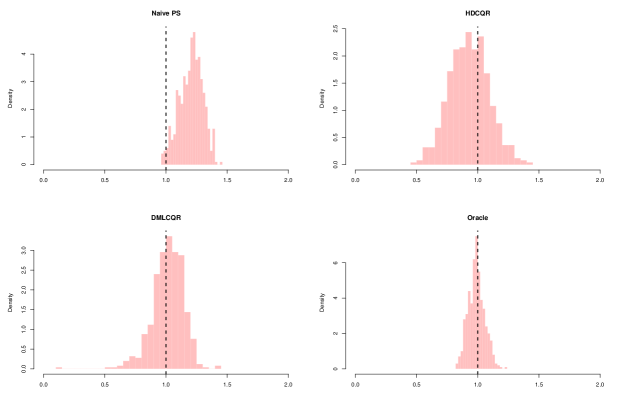
Figure 1: Histograms of simulation results

I now examine confidence intervals of different designs by varying

$$(R_{d}^{2},R_{y}^{2})\in\left\{0.1,0.2,0.3,0.4,0.5,0.6,0.7,0.8,0.9\right\}^{2},$$

which gives us 81 different designs. Figure 2 shows the rejection frequencies of confidence intervals with a nominal significance level of 5% for the Naive PS estimator and DMLCQR estimator with 2-fold cross-fitting. Ideally, the rejection rate should be the nomial level of 5% regardless of the underlying data generating process. The confidence regions for the Naive PS estimator deviate greatly from the ideal level, while those for the DMLCQR estimator are flat with a rejection rate close to the nominal level. Therefore, the simulation results demonstrate that the DMLCQR estimator has satisfactory finite sample performance compared to conventional alternatives.

Figure 2: Rejection probabilities of confidence regions with nominal coverage of 95%

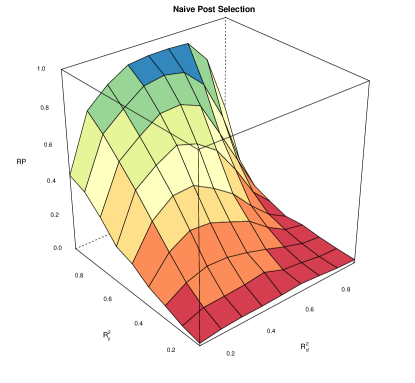
(a)

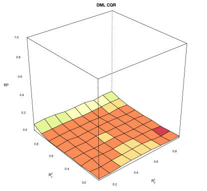
(b)

5 Empirical application

In this section, I apply the DML-CQR estimator to estimate the quantile treatment effect of 401(k) eligibility on total financial assets. Since working for a firm that offers a 401(k) plan is non-random, Poterba et al. (1994) and Poterba et al. (1995) developed a strategy that takes 401(k) eligibility as exogenous, after conditioning on control variables including income. They argued that when 401(k) plans were first introduced, people did not base their employment decisions on the availability of 401(k) plans, but instead focused on factors like income and other job characteristics. To validate the selection on observables assumption, a flexible set of controls that are correlated with both 401(k) eligibility and the outcome should be included. This led Belloni et al. (2017) and Chernozhukov et al. (2017a) to use high-dimensional controls and post-selection inference methods to study the effect of 401(k) eligibility on household’s net financial assets. They revisited previous empirical findings that assumed that the confounding effects could be adequately controlled for by a small number of ex ante chosen controls.

I conduct a similar study to Belloni et al. (2017) and Chernozhukov et al. (2017a), but using total financial asset as the outcome. In the data, 12.4 percent of households reported zero total financial assets, which is naturally bounded by zero, in contrast to the net financial assets, which can be negative. Although this is a corner solution outcome and not from bottom coding, we need to use an econometric model with a censored outcome to accurately incorporate the data structure. The treatment of interest is 401(k) eligibility, not participation, so the parameter of interest is the intent-to-treat effect. Poterba et al. (1995) conducted a median regression of 401(k) eligibility on total financial assets, but they did not consider that the outcome was censored and focused soley on the median quantile.

I use the same data as Chernozhukov and Hansen (2004). The data set consists of 9915 household-level observations obtained from the 1991 SIPP. Two households were removed due to reporting negative income, leaving a sample size of $N=9913$. The outcome variable $Y$ is total financial assets, which is defined as the sum of IRA balances, 401(k) balances, and other financial assets. The treatment variable $D$ is a binary indicator of eligibility to enroll in a 401(k) plan. The vector of raw covariates $X$ includes income, age, family size, years of education, marriage status indicator, a two-earner status indicator, a defined benefit pension status indicator, an IRA participation indicator, and home ownership indicator. Further information about the data can be found in Chernozhukov and Hansen (2004).

I consider three different sets of controls $f(X)$, modifying the specification outlined in Belloni et al. (2017). The first specification includes indicators of marriage status, two-earner status, defined benefit pension status, IRA participation, and home ownership status, as well as second-order polynomials in family size and education, a third-order polynomial in age, and a quadratic spline in income with six break points. The second specification adds interactions between all non-income variables and interactions between non-income variables and each term in the income spline to the first specification. The third specification augments interactions between interaction of non-incomevariables and the income terms. These three specifications are referred to as the low-p, high-p, and very high-p specifications, respectively. The dimensions of controls for the first, second, and third specifications are 20, 182, and 710. Additionally, I use 20, 157, and 498 variables for methods that do not use variable selection by removing perfectly collinear terms.

Figure 3 presents the quantile treatment effect estimates at quantiles $\tau=0.15,0.2,\dots,0.9$ and 95% confidence intervals. In the low-p specification, I apply conventional quantile regression and censored quantile regression estimator of Buchinsky and Hahn (1998) to compare whether the estimates change according to taking censored outcome into account in the model. The results indicate that using censored quantile regression model increases the QTE at lower quantiles closer to the censoring point. This makes sense as conditional quantiles at lower quantiles are more likely to be affected by censoring. Therefore, the result recommends the use of censored outcome models rather than ignoring the latent data structure. In the high-p specification, I compare the results using DMLCQR estimator and Buchinsky and Hahn (1998), where the latter could be understood as HDCQR estimator in the simulation. It shows that incorporating high-dimensional controls in Buchinsky and Hahn (1998) gives similar results to using quantile regression in the low-p specification, while DMLCQR estimates are consistent with estimates in the low-p specification accounting for censoring. This implies that implementing the conventional censored quantile regression estimator with high-dimensional control could lead to somewhat erratic estimates, close to using quantile regression with low-dimensional data. Lastly, the application of DMLCQR in the very high-p specification has similar results as in the high-p specification. As the results using DMLCQR with high-p and very high-p are very close to censored quantile regression estimates in the low-p, my result complements previous works that were based on the assumption that a small number of ex ante chosen controls are enough to control the confounding effect.

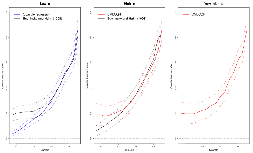
Figure 3: QTE estimates of the effect of 401(k) eligibility on total financial assets

6 Conclusion

Censored quantile regression has been popularly used in the causal inference literature. Some examples of its applications include the effect of tax incentives on charitable contributions (Fack and Landais (2010)), the effect of pollution on productivity (Graff Zivin and Neidell (2012)), and the price elasticity of medical expenditure (Kowalski (2016)). Empirical researchers frequently face the challenge of selecting important control variables from a rich set of potential controls, which could be alleviated by employing machine learning methods with regularization to estimate high-dimensional nuisance parameters. I propose the DMLCQR estimator, which improves upon the censored quantile regression estimator of Buchinsky and Hahn (1998), and enables researchers to use high-dimensional control variables while obtaining valid inference for the target parameter. This additional benefit makes censored quantile regression more practical for empirical researchers to analyze wider types of data sets and employ a broader set of machine learning methods for estimation.

Appendix

Notation

I work with triangular array data $\left\{\omega_{i,n};i=1,\dots,n;n=1,2,3,\dots\right\}$ where for each $n$, $\left\{\omega_{i,n};i=1,\dots,n\right\}$ is defined on the probability space $\left(\Omega,\mathcal{S},P_{n}\right)$. Each $\omega_{i,n}=(y_{i,n}^{\prime},d_{i,n}^{\prime},z_{i,n}^{\prime})^{\prime}$ is a vector which are independent across $i$ but not necessarily identically distributed (i.n.i.d.). Therefore, while all parameters that characterize the distribution of $\left\{\omega_{i,n};i=1,\dots,n\right\}$ are implicitly indexed by $P_{n}$ and $n$, I omit this dependence from the notation to maintain simplicity. I use the following notation: $E_{n}[f]=n^{-1}\sum_{i=1}^{n}f(\omega_{i})$, $\bar{E}_{n}[f]=E[E_{n}[f]]=\dfrac{1}{n}\sum_{i=1}^{n}E\left[f(\omega_{i})\right]$, and $\mathbb{G}_{n}(f(\omega_{i}))=\dfrac{1}{\sqrt{n}}\sum_{i=1}^{n}\left(f(\omega_{i})-E[f(\omega_{i})]\right)$. The $l_{2}$-norm is denoted by $\left\|\cdot\right\|$; the $l_{0}$-norm $\left\|\cdot\right\|_{0}$ denotes the number of nonzero components of a vector; and the $l_{\infty}$-norm $\left\|\cdot\right\|_{\infty}$ denotes the maximal absolute value in the components of a vector. For a sequence $\left(t_{i}\right)_{i=1}^{n}$, we denote $\left\|t_{i}\right\|_{2,n}=\sqrt{E_{n}\left[t_{i}^{2}\right]}$. We use the notation $a\lesssim b$ to denote $a\leq cb$ for some constant $c>0$ that does not depend on $n$; and $a\lesssim_{P}b$ to denote $a=O_{p}(b)$.

A Proof of the theoretical results

A.1 Proof of Lemma 1

Moment condition: From (2), the moment conditions for $\theta_{\tau}$ and $\beta_{\tau}$ are

$$E\left[\dfrac{\partial g(w_{i},\theta,\beta,\pi)}{\partial\theta}\right] =E\left[t_{i}I(h_{\tau i}>0)(h_{\tau i}-I(y_{i}-d_{i}\theta_{\tau}-x_{i}^{\prime}\beta_{\tau}\leq 0))d_{i}\right]=0$$ (11)

$$E\left[\dfrac{\partial g(w_{i},\theta,\beta,\pi)}{\partial\beta}\right] =E\left[t_{i}I(h_{\tau i}>0)(h_{\tau i}-I(y_{i}-d_{i}\theta_{\tau}-x_{i}^{\prime}\beta_{\tau}\leq 0))x_{i}\right]=0.$$ (12)

Therefore,

$$E\left[\psi(w_{i},\theta_{0},\eta_{0})\right] =E\left[I\left(h_{\tau i}>0\right)\left(t_{i}\left\{h_{\tau i}-I(y_{i}-d_{i}\theta_{\tau}-x_{i}^{\prime}\beta_{\tau}-r_{\tau i}\leq 0)\right\}+(t_{i}-\pi_{i})\dfrac{(1-\tau)}{\pi_{i}}\right)(d_{i}-x_{i}^{\prime}\mu_{\tau})\right]$$

$$=E\left[I\left(h_{\tau i}>0\right)t_{i}\left\{h_{\tau i}-I(y_{i}-d_{i}\theta_{\tau}-x_{i}^{\prime}\beta_{\tau}-r_{\tau i}\leq 0)\right\}d_{i}\right]$$

$$\;-E\left[I\left(h_{\tau i}>0\right)t_{i}\left\{h_{\tau i}-I(y_{i}-d_{i}\theta_{\tau}-x_{i}^{\prime}\beta_{\tau}-r_{\tau i}\leq 0)\right\}x_{i}^{\prime}\mu_{\tau}\right]$$

$$\;+E\left[(t_{i}-\pi_{i})I\left(h_{\tau i}>0\right)\dfrac{(1-\tau)}{\pi_{i}}(d_{i}-x_{i}^{\prime}\mu_{\tau})\right]$$

$$=E\left[(t_{i}-\pi_{i})I\left(h_{\tau i}>0\right)\dfrac{(1-\tau)}{\pi_{i}}(d_{i}-x_{i}^{\prime}\mu_{\tau})\right]\;(\because(6),(7))$$

$$=E\left[E[t_{i}-\pi_{i}|w_{i}]I\left(h_{\tau i}>0\right)\dfrac{(1-\tau)}{\pi_{i}}(d_{i}-x_{i}^{\prime}\mu_{\tau})\right]\;(\because\text{Law of iterated expectations})$$

$$=0$$

and the moment condition $E\left[\psi(w_{i},\theta_{0},\eta_{0})\right]=0$ holds.

Neyman orthogonality: The pathwise derivative of (4) in the direction $\eta-\eta_{0}=(\pi-\pi_{0},\beta-\beta_{\tau},\mu-\mu_{\tau})$ is

$$\partial_{\pi}E\left[\psi(w_{i},\theta_{0},\eta_{0})\right][\pi-\pi_{0}]$$

$$=E\left[\left\{t_{i}I\left(h_{i}>0\right)\dfrac{1-\tau}{\pi_{i}^{2}}(d_{i}-x_{i}^{\prime}\mu_{\tau})-t_{i}I\left(h_{i}>0\right)\dfrac{1-\tau}{\pi_{i}^{2}}(d_{i}-x_{i}^{\prime}\mu_{\tau})\right\}\left(\pi_{i}-\pi_{0i}\right)\right]=0$$

$$\partial_{\beta}E\left[\psi(w_{i},\theta_{0},\eta_{0})\right][\beta-\beta_{\tau 0}]$$

$$=\partial_{r}E\left[I\left(h_{\tau i}>0\right)\left(t_{i}\left\{h_{\tau i}-P(y_{i}-d_{i}\theta_{\tau}-x_{i}^{\prime}\beta_{\tau}-r_{\tau i}\leq x_{i}^{\prime}(\tilde{\beta}-\beta_{\tau})|w_{i})\right\}+(t_{i}-\pi_{i})\dfrac{(1-\tau)}{\pi_{i}}\right)(d_{i}-x_{i}^{\prime}\mu_{\tau})\right]\Big{|}_{r=0}$$

$$=-E\left[I\left(h_{\tau i}>0\right)t_{i}f(x_{i}^{\prime}(\tilde{\beta}-\beta_{\tau})|w_{i})(d_{i}-x_{i}^{\prime}\mu_{\tau})x_{i}^{\prime}\left(\beta-\beta_{\tau}\right)\right]\Big{|}_{r=0}$$

$$=-E\left[t_{i}I\left(h_{i}>0\right)f_{i}(d_{i}-x_{i}^{\prime}\mu_{\tau})x_{i}^{\prime}\left(\beta-\beta_{\tau}\right)\right]=0\;(\because\text{Definition of $\mu_{\tau}$})$$

$$=0$$

$$\partial_{\mu}E\left[\psi(w_{i},\theta_{0},\eta_{0})\right][\mu-\mu_{\tau 0}]$$

$$=-E\left[t_{i}I\left(h_{i}>0\right)\left(h_{i}-I\left\{y_{i}\leq d_{i}\theta_{\tau}+x_{i}^{\prime}\beta_{\tau}+r_{\tau i}\right\}\right)x_{i}^{\prime}\left(\mu-\mu_{\tau}\right)\right]-E\left[(t_{i}-\pi_{i})I\left(h_{i}>0\right)\dfrac{(1-\tau)}{\pi_{i}}x_{i}^{\prime}\left(\mu-\mu_{\tau}\right)\right]$$

$$=-E\left[t_{i}I\left(h_{i}>0\right)\left(h_{i}-F_{y}\left\{d_{i}\theta_{\tau}+x_{i}^{\prime}\beta_{\tau}+r_{\tau i}|w_{i},t_{i}=1,\pi_{i}>1-\tau\right\}\right)x_{i}^{\prime}\tilde{\mu}\right]$$

$$\;\;-E\left[E[t_{i}-\pi_{i}|w_{i}]\cdot I\left(h_{i}>0\right)\dfrac{(1-\tau)}{\pi_{i}}x_{i}^{\prime}\tilde{\mu}\right]=0.$$

A.2 Assumption IQR

I suppress $\tau$ notation in the parameters for the sake of simplicity.

A.2.1 Assumption

For $k\in[K]$, I assume that

$$L_{n}(\check{\theta}_{k})\leq\min_{\theta\in\Theta_{\tau}}L_{n}(\theta)+\delta_{n}n^{-1}.$$

I suppress $k$ notation in the parameters. We define

$$\Gamma(\tilde{\theta},\tilde{\eta}) =\bar{E}\left[\psi_{\theta,\eta}(y_{i},d_{i},x_{i})\right]|_{\theta=\tilde{\theta},h=\tilde{\eta}}$$

$$\Gamma_{\eta}(\tilde{\theta},\tilde{\eta})[\hat{\eta}-\eta_{0}] =\lim_{t\to 0}\dfrac{\Gamma(\tilde{\theta},\tilde{\eta}+t[\hat{\eta}-\eta_{0}])-\Gamma(\tilde{\theta},\tilde{\eta})}{t}$$

where $\Gamma_{\eta}$ is the directional derivative with respect to $[\hat{\eta}-\eta_{0}]$ at $(\tilde{\theta},\tilde{\eta})$.

We denote the nuisance parameters as $\eta=(g,v,\pi)$ where $v_{i}=d_{i}-x_{i}^{\prime}\mu$. We define the score with $(\theta,\eta)$ as

$$\psi_{\theta,\eta}(w_{i}) =I\left(h_{i}>0\right)\left(t_{i}\left\{h_{i}-I(y_{i}-d_{i}\theta-g_{i}\leq 0)\right\}+(t_{i}-\pi_{i})\dfrac{(1-\tau)}{\pi_{i}}\right)v_{i}.$$ (13)

For some sequences $\delta_{n}\to 0$ and $\Delta_{n}\to 0$, we let $\overline{\mathcal{F}}$ denote a set of functions such that each element $\tilde{\eta}=(\tilde{g},\tilde{v},\tilde{\pi})\in\overline{\mathcal{F}}$ satisfies

$$\bar{E}\left[(\tilde{g}_{i}-g_{i})^{2}\right] \lesssim\delta_{n}n^{-1/2}$$ (14)

$$\left|\bar{E}[f_{i}v_{i}\{\tilde{g}_{i}-g_{i}\}]\right| \leq\delta_{n}n^{-1/2}$$ (15)

$$\bar{E}[(\tilde{v}_{i}-v_{i})^{2}] \leq\delta_{n}$$ (16)

$$\bar{E}[\left|\tilde{g}_{i}-g_{i}\right|\left|\tilde{v}_{i}-v_{i}\right|] \leq\delta_{n}n^{-1/2}$$ (17)

$$\bar{E}\left[\left|v_{i}\right|(\tilde{g}_{i}-g_{i})^{2}\right] \leq\delta_{n}n^{-1/2}$$ (18)

$$\bar{E}\left[\left|\tilde{v}_{i}-v_{i}\right|(\tilde{g}_{i}-g_{i})^{2}\right] \leq\delta_{n}n^{-1/2}$$ (19)

and with probability $1-\Delta_{n}$ we have

$$\sup_{|\theta-\theta_{0}|\leq\delta_{n}^{2},\tilde{\eta}\in\mathcal{\overline{\mathcal{F}}}}\left|(E_{n}-\bar{E})[\psi_{\theta,\tilde{\eta}}-\psi_{\theta,\eta_{0}}]\right|\leq\delta_{n}n^{-1/2}.$$ (20)

We assume the estimated functions $\hat{\eta}=(\hat{g},\hat{v},\hat{\pi})$ satisfy the following condition.

Condition IQR. Let $\{(y_{i},d_{i},z_{i})\}$ be random variables independent across $i$ satisfying (1) and (5). Suppose there are positive constants $0<c\leq C<\infty$ such that:

(1) $f_{y_{i}|d_{i},z_{i}}(y|d_{i},z_{i})\leq\bar{f}$, $f_{y_{i}|d_{i},z_{i}}^{\prime}(y|d_{i},z_{i})\leq\bar{f^{\prime}}$; $\bar{E}[v_{i}^{4}]+\bar{E}[d_{i}^{4}]\leq C$; $c\leq|\bar{E}[t_{i}I\left(h_{i}>0\right)f_{i}d_{i}v_{i}]|$

(2) $\left\{\theta:|\theta-\theta_{0}|\leq n^{-1/2}/\delta_{n}\right\}\subset\Theta_{\tau}$ where $\Theta_{\tau}$ is a (possibly random) compact interval.

(3) with probability at least $1-\Delta_{n}$ the estimated functions $\hat{\eta}=(\hat{g},\hat{v},\hat{\pi})\in\overline{\mathcal{F}}$ and

$$|\check{\theta}-\theta_{0}|\leq\delta_{n}\;\text{and }E_{n}[\psi_{\check{\theta},\hat{\eta}}(y_{i},d_{i},z_{i})]\leq\delta_{n}n^{-1/2}.$$

(4) with probability at least $1-\Delta_{n}$ the estimated functions $\hat{\eta}=(\hat{g},\hat{v},\hat{\pi})$ satisfy

$$\left\|\hat{v}_{i}-v_{i}\right\|_{2,n} \leq\delta_{n}$$ (21)

$$\left\|\hat{\pi}_{i}-\pi_{i}\right\|_{2,n} \leq\delta_{n}$$ (22)

$$\left\|I\left(\hat{h}_{i}>0\right)-I\left(h_{i}>0\right)\right\|_{2,n} \leq\delta_{n}$$ (23)

$$\left\|I\left(\left|\epsilon_{i}\right|\leq\left|d_{i}(\theta-\check{\theta})+g_{i}-\hat{g}_{i}\right|\right)\right\|_{2,n} \leq\delta_{n}^{2}.$$ (24)

A.2.2 Proof

Condition IQR (1) requires conditions on the probability density function that are assumed in Condition AS (3). $\bar{E}[v_{i}^{4}]+\bar{E}[d_{i}^{4}]\leq C$ is implied by Condition M (1) using $\xi_{1}=(1,0^{\prime})^{\prime}$ and $\xi_{2}=(1,-\mu_{\tau}^{\prime})^{\prime}$ since $\bar{E}[d_{i}^{4}]=\bar{E}[\{(d_{i},x_{i}^{\prime})\xi_{1}\}^{4}]\leq C$ and $\bar{E}[v_{i}^{4}]\leq\bar{E}[\{(d_{i},x_{i}^{\prime})\xi_{2}\}^{4}]\leq C(1+\left\|\mu_{\tau}\right\|)^{4}$ and $\left\|\mu_{\tau}\right\|\leq C$ as assumed in Condition AS (1). $c\leq|\bar{E}[t_{i}I\left(h_{i}>0\right)f_{i}d_{i}v_{i}]|$ is implied by $\bar{E}[t_{i}I\left(h_{i}>0\right)f_{i}d_{i}v_{i}]=\bar{E}[t_{i}I\left(h_{i}>0\right)f_{i}v_{i}^{2}]\geq\underline{f}$.

Condition IQR (3): I first verify $\hat{\eta}=(\hat{g},\hat{v},\hat{\pi})\in\overline{\mathcal{F}}$. Belloni et al. (2019) show $\bar{E}\left[\left\{x_{i}^{\prime}(\tilde{\beta}-\beta)\right\}^{2}\right]\lesssim_{P}\sqrt{\dfrac{s\log(pn)}{n}}$ and $\bar{E}[\left\{x_{i}^{\prime}(\tilde{\mu}-\mu)\right\}^{2}]\lesssim\dfrac{1}{h^{2}}\dfrac{s\log(pn)}{n}+h^{2\bar{k}}+\dfrac{\lambda^{2}}{n^{2}}s$where $h$ is the bandwidth for estimating $\hat{f}_{i}$. I verify equation (9) to (14) under conditions.

$$\bar{E}\left[(\tilde{g}_{i}-g_{i})^{2}\right]\leq\bar{E}\left[\left\{x_{i}^{\prime}(\tilde{\beta}-\beta)\right\}^{2}\right]+\bar{E}\left[r_{i}^{2}\right]\lesssim\dfrac{s\log(pn)}{n}\lesssim\delta_{n}n^{-1/2}\;(\because\text{Condition AS (2)})$$

$$\left|\bar{E}[t_{i}I\left(h_{i}>0\right)f_{i}v_{i}(\tilde{g}_{i}-g_{i})]\right| \leq\left|\bar{E}[t_{i}I\left(h_{i}>0\right)f_{i}v_{i}x_{i}^{\prime}(\tilde{\beta}-\beta)]\right|+\left|\bar{E}[t_{i}I\left(h_{i}>0\right)f_{i}v_{i}r_{i}]\right|$$

$$=\left|\bar{E}[t_{i}I\left(h_{i}>0\right)\sqrt{f}_{i}u_{i}x_{i}^{\prime}(\tilde{\beta}-\beta)]\right|+\left|\bar{E}[t_{i}I\left(h_{i}>0\right)f_{i}v_{i}r_{i}]\right|$$

$$=\left|\bar{E}[t_{i}I\left(h_{i}>0\right)f_{i}v_{i}r_{i}]\right|\;(\because\bar{E}[t_{i}I(h_{\tau i}>0)\sqrt{f_{i}}x_{i}u_{i}]=0)$$

$$\lesssim\delta_{n}n^{-1/2}\;(\because\text{Condition M (2)})$$

$$\bar{E}[(\tilde{v}_{i}-v_{i})^{2}]=\bar{E}[\left\{x_{i}^{\prime}(\tilde{\mu}-\mu)\right\}^{2}]\lesssim\dfrac{1}{h^{2}}\dfrac{s\log(pn)}{n}+h^{2\bar{k}}+\dfrac{\lambda^{2}}{n^{2}}s\lesssim\delta_{n}$$

under $h^{-2}s\log(pn)\leq\delta_{n}n$, $h\leq\delta_{n}$, and $\lambda^{2}s\leq\delta_{n}n^{2}$.

$$\bar{E}[\left|\tilde{g}_{i}-g_{i}\right|\left|\tilde{v}_{i}-v_{i}\right|] =\bar{E}[\left|\tilde{g}_{i}-g_{i}\right|\left|x_{i}^{\prime}(\tilde{\mu}-\mu)\right|]$$

$$\leq\bar{E}[(\tilde{g}_{i}-g_{i})^{2}]^{1/2}\bar{E}[\left\{x_{i}^{\prime}(\tilde{\mu}-\mu)\right\}^{2}]^{1/2}$$

$$\lesssim\left\{s\log(pn)/n\right\}^{1/2}\left\{\dfrac{1}{h}\sqrt{\dfrac{s\log(pn)}{n}}+h^{\bar{k}}+\lambda\dfrac{\sqrt{s}}{n}\right\}\lesssim\delta_{n}n^{-1/2}$$

under $h^{-2}s^{2}\log^{2}(pn)\leq\delta_{n}^{2}n$ and $h^{\bar{k}}\sqrt{s\log(pn)}\leq\delta_{n}$.

$$\bar{E}\left[\left|v_{i}\right|(\tilde{g}_{i}-g_{i})^{2}\right] =\bar{E}\left[\left|v_{i}\right|\left\{x_{i}^{\prime}(\tilde{\beta}-\beta)\right\}^{2}\right]+\bar{E}\left[\left|v_{i}\right|r_{i}^{2}\right]$$

$$\leq\left(\bar{E}\left[v_{i}^{2}\left\{x_{i}^{\prime}(\tilde{\beta}-\beta)\right\}^{2}\right]\bar{E}\left[\left\{x_{i}^{\prime}(\tilde{\beta}-\beta)\right\}^{2}\right]\right)^{1/2}+\left(\bar{E}\left[v_{i}^{2}r_{i}^{2}\right]\bar{E}\left[r_{i}^{2}\right]\right)^{1/2}$$

$$\lesssim\left\{s\log(pn)/n\right\}^{1/2}\left\{\bar{E}\left[v_{i}^{2}\left\{x_{i}^{\prime}(\tilde{\beta}-\beta)\right\}^{2}\right]+\bar{E}\left[v_{i}^{2}r_{i}^{2}\right]\right\}^{1/2}$$

$$\lesssim s\log(pn)/n\lesssim\delta_{n}n^{-1/2}$$

since $\left\|(1,-\mu)\right\|\leq C$, $\bar{E}[\{(d_{i},x_{i}^{\prime})\xi\}^{4}]\leq C\left\|\xi\right\|^{4}$, and $\bar{E}\left[\left(x_{i}^{\prime}\xi\right)^{2}r_{\tau i}^{2}\right]\leq C\left\|\xi\right\|^{2}\bar{E}\left[r_{\tau i}^{2}\right]$. Lastly,

$$\bar{E}\left[\left|\tilde{v}_{i}-v_{i}\right|(\tilde{g}_{i}-g_{i})^{2}\right] =\bar{E}\left[\left|x_{i}^{\prime}(\tilde{\mu}-\mu)\right|(\tilde{g}_{i}-g_{i})^{2}\right]$$

$$=\bar{E}\left[\left|x_{i}^{\prime}(\tilde{\mu}-\mu)\right|(\tilde{g}_{i}-g_{i})^{2}\right]$$

$$\lesssim s\log(pn)/n\lesssim\delta_{n}n^{-1/2}.$$

Next, I verify equation (20). Let $\mathcal{F}_{1,\eta}=\left\{\psi_{\theta,\eta}:\left|\theta-\theta_{0}\right|\leq\delta_{n}^{2}\right\}$ and $\mathcal{F}_{2}=\left\{\psi_{\theta,\tilde{\eta}}-\psi_{\theta,\eta_{0}}:\left|\theta-\theta_{0}\right|\leq\delta_{n}^{2}\right\}$. Note that $\mathcal{F}_{2}\subset\mathcal{F}_{1,\tilde{\eta}}-\mathcal{F}_{1,\eta}$. Since $\mathcal{F}_{1,\eta}$ is the produce of a VC class of dimension 1 with the random variable $v$, its entropy nuber satisfies $\log N\left(\epsilon\left\|F_{1,\eta}\right\|_{Q,2},\mathcal{F}_{1,\eta},\left\|\cdot\right\|_{Q,2}\right)\leq v\log(a/\epsilon)$ where $F_{1,\eta}$ is a measurable envelope for $\mathcal{F}_{1,\eta}$ that satisfies $\left\|F_{1,\eta}\right\|_{P,q}\leq c_{1}$. Therefore, $\left\|F_{2}\right\|_{P,q}=\left\|F_{1,\eta}\right\|_{P,q}+\left\|F_{1,\tilde{\eta}}\right\|_{P,q}\leq 2c_{1}$ by the triangle inequality and $\log N\left(\epsilon\left\|F_{2}\right\|_{Q,2},\mathcal{F}_{2},\left\|\cdot\right\|_{Q,2}\right)\leq 2v\log(2a/\epsilon)$ by the proof of Theorem 3 in Andrews (1994). To bound $\sup_{f\in\mathcal{F}_{2}}\left|\mathbb{G}_{n}(f)\right|$, I apply Theorem 5.1 of Chernozhukov et al. (2014) conditional on $(w_{i})_{i\in I^{c}}$ so that $\tilde{\eta}$ can be treated as fixed. By the proof of Theorem 2 in Section A.5, note that for $f_{2}\in\mathcal{F}_{2}$,

$$\left\|f_{2}\right\|_{P,2}^{2}$$

$$=\bar{E}\left[\left\{\psi(w_{i},\theta,\tilde{\eta})-\psi(w_{i},\theta,\eta_{0})\right\}^{2}\right]$$

$$\lesssim\bar{E}\left[(\hat{v}_{i}-v_{i})^{2}\right]+\bar{E}\left[(\hat{\pi}_{i}-\pi_{i})^{2}\right]+\bar{E}\left[\left(I\left(\hat{h}_{i}>0\right)-I\left(h_{i}>0\right)\right)^{2}\right]+\bar{E}\left[v_{i}^{2}I\left(\left|\epsilon_{i}\right|\leq\left|d_{i}(\theta-\tilde{\theta})+g_{i}-\tilde{g}_{i}\right|\right)^{2}\right]$$

$$\lesssim\dfrac{1}{h^{2}}\dfrac{s\log(pn)}{n}+h^{2\bar{k}}+\dfrac{\lambda^{2}}{n^{2}}s.$$

Applying the theorem with with $\sigma=C\left\{\dfrac{1}{h}\sqrt{\dfrac{s\log(pn)}{n}}+h^{\bar{k}}+\dfrac{\lambda}{n}\sqrt{s}\right\}$,$a=pn$, $v=s$, $\left\|M\right\|_{P,2}\leq C$ yields

$$\sup_{|\theta-\theta_{0}|\leq\delta_{n}^{2},\tilde{\eta}\in\mathcal{\overline{\mathcal{F}}}}\left|(E_{n}-\bar{E})[\psi_{\theta,\tilde{\eta}}-\psi_{\theta,\eta_{0}}]\right| \lesssim\dfrac{1}{\sqrt{n}}\left\{\left(\dfrac{1}{h}\sqrt{\dfrac{s\log(pn)}{n}}+h^{\bar{k}}+\dfrac{\lambda}{n}\sqrt{s}\right)\sqrt{s\log(pn)}+\dfrac{1}{\sqrt{n}}sC\log(pn)\right\}$$

$$\lesssim\delta_{n}n^{-1/2}.$$

Condition IQR (4): I verify equations (16) to (19).

$$\left\|\hat{v}_{i}-v_{i}\right\|_{2,n}\lesssim_{P}\bar{E}\left[(\hat{v}_{i}-v_{i})^{2}\right]^{1/2}\lesssim\delta_{n}^{1/2}$$

$$\left\|\hat{\pi}_{i}-\pi_{i}\right\|_{2,n}\lesssim_{P}\bar{E}\left[(\hat{\pi}_{i}-\pi_{i})^{2}\right]^{1/2}\lesssim\sqrt{\dfrac{s\ln(pn)}{n}}=\delta_{n}$$

$$\left\|I\left(\hat{h}_{i}>0\right)-I\left(h_{i}>0\right)\right\|_{2,n} =\left\|I\left(\hat{\pi}_{i}>1-\tau\right)-I\left(\pi_{i}>1-\tau\right)\right\|_{2,n}$$

$$=\sqrt{\dfrac{1}{n}\sum_{i=1}^{n}\left\{I\left(\hat{\pi}_{i}>1-\tau\right)-I\left(\pi_{i}>1-\tau\right)\right\}^{2}}$$

Note that

$$\left|I\left(\hat{\pi}_{i}>1-\tau\right)-I\left(\pi_{i}>1-\tau\right)\right| =\left|I\left(\pi_{i}-\varepsilon_{i}>1-\tau\right)-I\left(\pi_{i}>1-\tau\right)\right|\;(\because\varepsilon_{i}=\hat{\pi}_{i}-\pi_{i})$$

$$=\left|I(\iota_{i}>\varepsilon_{i})-I(\iota_{i}>0)\right|\;(\because\iota_{i}=\pi_{i}-(1-\tau))$$

$$\leq I(\left|\iota_{i}\right|<\left|\varepsilon_{i}\right|).$$

Therefore,

$$\left\|I\left(\hat{\pi}_{i}>1-\tau\right)-I\left(\pi_{i}>1-\tau\right)\right\|_{2,n}^{2} \leq\dfrac{1}{n}\sum_{i=1}^{n}I(\left|\iota_{i}\right|<\left|\hat{\pi}_{i}-\pi_{i}\right|)$$

$$\lesssim_{P}\bar{E}\left[I(\left|\iota_{i}\right|<\left|\hat{\pi}_{i}-\pi_{i}\right|)\right]$$

$$\leq\bar{f}_{\iota}\dfrac{1}{n}\sum_{i=1}^{n}\left|\hat{\pi}_{i}-\pi_{i}\right|\lesssim\sqrt{\dfrac{1}{n}\sum_{i=1}^{n}\left(\hat{\pi}_{i}-\pi_{i}\right)^{2}}\lesssim_{P}\sqrt{\dfrac{s\ln(pn)}{n}}=\delta_{n}.$$

$$\left\|I\left(\left|\epsilon_{i}\right|\leq\left|d_{i}(\theta-\check{\theta})+g_{i}-\tilde{g}_{i}\right|\right)\right\|_{2,n}^{2} =E_{n}\left[I\left(\left|\epsilon_{i}\right|\leq\left|d_{i}(\theta-\tilde{\theta})\right|\right)\right]+E_{n}\left[I\left(\left|\epsilon_{i}\right|\leq\left|x_{i}^{\prime}(\tilde{\beta}-\beta)\right|\right)\right]+E_{n}\left[I\left(\left|\epsilon_{i}\right|\leq\left|r_{i}\right|\right)\right]$$

$$\lesssim_{P}\bar{E}\left[I\left(\left|\epsilon_{i}\right|\leq\left|d_{i}(\theta-\tilde{\theta})\right|\right)\right]+\bar{E}\left[I\left(\left|\epsilon_{i}\right|\leq\left|x_{i}^{\prime}(\tilde{\beta}-\beta)\right|\right)\right]+\bar{E}\left[\left|\epsilon_{i}\right|\leq\left|r_{i}\right|\right]$$

$$\leq\bar{f}\left\{\dfrac{1}{n}\sum_{i=1}^{n}\left|d_{i}(\theta-\tilde{\theta})\right|+\dfrac{1}{n}\sum_{i=1}^{n}\left|x_{i}^{\prime}(\tilde{\beta}-\beta)\right|+\dfrac{1}{n}\sum_{i=1}^{n}\left|r_{i}\right|\right\}$$

$$\leq\bar{f}\left\{\sqrt{\dfrac{1}{n}\sum_{i=1}^{n}\left|d_{i}(\theta-\tilde{\theta})\right|^{2}}+\sqrt{\dfrac{1}{n}\sum_{i=1}^{n}\left|x_{i}^{\prime}(\tilde{\beta}-\beta)\right|^{2}}+\sqrt{\dfrac{1}{n}\sum_{i=1}^{n}\left|r_{i}\right|^{2}}\right\}$$

$$\lesssim_{P}\bar{f}\left\{\left|\theta-\tilde{\theta}\right|\sqrt{\bar{E}[d_{i}^{2}]}+\sqrt{\bar{E}\left[\left|x_{i}^{\prime}(\tilde{\beta}-\beta)\right|^{2}\right]}+\sqrt{\bar{E}\left[\left|r_{i}\right|^{2}\right]}\right\}$$

$$\lesssim\bar{f}\sqrt{\dfrac{s\ln(pn)}{n}}=\delta_{n}$$

A.3 Proof of Theorem 1 (DML 1 case)

A.3.1 Lemma

Lemma 2.

Under the condition IQR, we have for all $k\in[K]$,

$$\bar{\sigma}_{n}^{-1}\sqrt{n}(\check{\theta}_{k}-\theta)=\bar{E}_{n}\left[\psi^{2}(w_{i},\theta_{0},\eta_{0})\right]^{-1/2}\dfrac{1}{\sqrt{n}}\sum_{i\in I_{k}}\psi(w_{i},\theta_{0},\eta_{0})\overset{d}{\to}N(0,1)$$

where $\bar{\sigma}_{n}^{2}=\left(\bar{E}_{n}[t_{i}I(h_{i}>0)f_{i}d_{i}v_{i}]\right)^{-1}\bar{E}_{n}\left[\psi^{2}(w_{i},\theta_{0},\eta_{0})\right]\left(\bar{E}_{n}[t_{i}I(h_{i}>0)f_{i}d_{i}v_{i}]\right)^{-1}$.

Proof.

In the proof, I use $(\check{\theta},\hat{h})$ instead of $(\check{\theta}_{k},\hat{h}_{k})$.

Step 1. Normality result

We have the following identity

$$E_{n}[\psi_{\check{\theta},\hat{\eta}}] =E_{n}[\psi_{\theta_{0},\eta_{0}}]+E_{n}[\psi_{\check{\theta},\hat{\eta}}-\psi_{\theta_{0},\eta_{0}}]$$

$$=E_{n}[\psi_{\theta_{0},\eta_{0}}]+\underbrace{\bar{E}[\psi_{\check{\theta},\hat{\eta}}]}_{(1)}+\underbrace{n^{-1/2}\mathbb{G}_{n}(\psi_{\check{\theta},\hat{\eta}}-\psi_{\check{\theta},\eta_{0}})}_{(2)}+\underbrace{n^{-1/2}\mathbb{G}_{n}(\psi_{\check{\theta},\eta_{0}}-\psi_{\theta_{0},\eta_{0}})}_{(3)}.$$

By the second relation in IQR (3), the left hand side satisfies $\left|E_{n}[\psi_{\check{\theta},\hat{\eta}}]\right|\lesssim\delta_{n}n^{-1/2}$ with probability at least $1-\Delta_{n}$. By step 2, $(1)=-\bar{E}\left[t_{i}I\left(h_{i}>0\right)f_{i}d_{i}v_{i}\right](\hat{\theta}-\theta_{0})+O(\delta_{n}n^{-1/2}+\delta_{n}\left|\hat{\theta}-\theta_{0}\right|)$. Since $\hat{\eta}=(\hat{g},\hat{v},\hat{\pi})\in\overline{\mathcal{F}}$ with probability at least $1-\Delta_{n}$ by IQR (3), equation (15) holds. By condition IQR (3) we have with probability at least $1-\Delta_{n}$ that $|\check{\theta}-\theta_{0}|\leq\delta_{n}$. Therefore, we can apply equation (15) and we have $\left|(2)\right|\lesssim\delta_{n}n^{-1/2}$. By condition IQR (3) we have with probability at least $1-\Delta_{n}$ that $|\check{\theta}-\theta_{0}|\leq\delta_{n}$. Observe that

$$(\psi_{\theta,\eta_{0}}-\psi_{\theta_{0},\eta_{0}})(y_{i},d_{i},z_{i}) =t_{i}I\left(h_{i}>0\right)\left(I(y_{i}-d_{i}\theta_{0}-g_{i}\leq 0)-I(y_{i}-d_{i}\theta-g_{i}\leq 0)\right)v_{i}$$

$$=t_{i}I\left(h_{i}>0\right)\left(I(\epsilon_{i}\leq 0)-I(\epsilon_{i}\leq d_{i}(\theta-\theta_{0}))\right)v_{i}$$

so that $\left|(\psi_{\theta,\eta_{0}}-\psi_{\theta_{0},\eta_{0}})(y_{i},d_{i},z_{i})\right|\leq I\left\{\left|\epsilon_{i}\right|\leq\delta_{n}\left|d_{i}\right|\right\}\left|v_{i}\right|$ whenever $|\theta-\theta_{0}|\leq\delta_{n}$. Since the class of functions

$\left\{(y,d,z)\mapsto(\psi_{\theta,\eta_{0}}-\psi_{\theta_{0},\eta_{0}})(y,d,z):|\theta-\theta_{0}|\leq\delta_{n}\right\}$ is a VC subgraph class, we have

$$\sup_{|\theta-\theta_{0}|\leq\delta_{n}}\left|\mathbb{G}_{n}(\psi_{\theta,\eta_{0}}-\psi_{\theta_{0},\eta_{0}})\right|\lesssim\left(\bar{E}\left[I\left\{\left|\epsilon_{i}\right|\leq\delta_{n}\left|d_{i}\right|\right\}v_{i}^{2}\right]\right)^{1/2}\lesssim\delta_{n}^{1/2}.$$

This implies that $\left|(3)\right|\lesssim\delta_{n}^{1/2}n^{-1/2}$ with probability $1-o(1)$.

Combining these relations we have

$$\bar{E}\left[t_{i}I\left(h_{i}>0\right)f_{i}d_{i}v_{i}\right](\hat{\theta}-\theta_{0}) =E_{n}[\psi_{\theta_{0},h_{0}}]+O_{p}(\delta_{n}n^{-1/2})+O_{p}(\delta_{n})\left|\hat{\theta}-\theta_{0}\right|$$

$$\sqrt{n}(\hat{\theta}-\theta_{0})\left\{\bar{E}\left[t_{i}I\left(h_{i}>0\right)f_{i}d_{i}v_{i}\right]-O_{p}(\delta_{n})\right\} =\sqrt{n}E_{n}[\psi_{\theta_{0},h_{0}}]+O_{p}(\delta_{n}).$$

Note that by the Lyapunov CLT

$$\dfrac{\sqrt{n}E_{n}[\psi_{\theta_{0},h_{0}}]}{\bar{E}[\psi_{\theta_{0},h_{0}}^{2}]^{1/2}}\overset{d}{\to}N(0,1)$$

∎

$$\bar{\sigma}_{n}^{-1}\sqrt{n}(\theta-\theta_{0})=\dfrac{\sqrt{n}E_{n}[\psi_{\theta_{0},h_{0}}]}{\bar{E}[\psi_{\theta_{0},h_{0}}^{2}]^{1/2}}\overset{d}{\to}N(0,1)$$

where $\bar{\sigma}_{n}^{2}=\bar{E}\left[t_{i}I\left(h_{i}>0\right)f_{i}d_{i}v_{i}\right]^{-1}\bar{E}[\psi_{\theta_{0},h_{0}}^{2}]\bar{E}\left[t_{i}I\left(h_{i}>0\right)f_{i}d_{i}v_{i}\right]^{-1}$ by $\bar{E}\left[t_{i}I\left(h_{i}>0\right)f_{i}d_{i}v_{i}\right]\geq c$ in IQR (1).

Step 2. $(1)=-\bar{E}\left[t_{i}I\left(h_{i}>0\right)f_{i}d_{i}v_{i}\right](\theta-\theta_{0})+O(\delta_{n}\left|\theta-\theta_{0}\right|C+\delta_{n}n^{-1/2})$

Step 2-1. Bounding $\Gamma(\theta,\hat{\eta})$ for $\left|\theta-\theta_{0}\right|\leq\delta_{n}$

For any (fixed function) $\hat{\eta}\in\overline{\mathcal{F}}$, we have

$$\bar{E}[\psi_{\theta,\hat{\eta}}] =\bar{E}[\psi_{\theta,\eta_{0}}]+\bar{E}[\psi_{\theta,\hat{\eta}}]-\bar{E}[\psi_{\theta,\eta_{0}}]$$

$$=\bar{E}[\psi_{\theta,\eta_{0}}]+\left\{\bar{E}[\psi_{\theta,\hat{\eta}}]-\bar{E}[\psi_{\theta,\eta_{0}}]-\Gamma_{\eta}(\theta,\eta_{0})(\hat{\eta}-\eta_{0})\right\}+\Gamma_{\eta}(\theta,\eta_{0})(\hat{\eta}-\eta_{0})$$

$$=\underbrace{\bar{E}[\psi_{\theta,\eta_{0}}]}_{(a)}+\underbrace{\left\{\bar{E}[\psi_{\theta,\hat{\eta}}]-\bar{E}[\psi_{\theta,\eta_{0}}]-\Gamma_{\eta}(\theta,\eta_{0})(\hat{\eta}-\eta_{0})\right\}}_{(b)}+\underbrace{\Gamma_{\eta}(\theta_{0},\eta_{0})[\hat{\eta}-\eta_{0}]}_{(c)}$$

$$\;\;+\underbrace{\left\{\Gamma_{\eta}(\theta,\eta_{0})[\hat{\eta}-\eta_{0}]-\Gamma_{\eta}(\theta_{0},\eta_{0})[\hat{\eta}-\eta_{0}]\right\}}_{(d)}.$$

$(a)$: By Taylor expansion, there is some $\tilde{\theta}\in[\theta_{0},\theta]$ such that

$$\bar{E}[\psi_{\theta,\eta_{0}}]=\Gamma(\theta_{0},\eta_{0})+\Gamma_{\theta}(\tilde{\theta},\eta_{0})(\theta-\theta_{0})=\left\{\Gamma_{\theta}(\theta_{0},\eta_{0})+\eta_{n}\right\}(\theta-\theta_{0})$$

where $\left|\eta_{n}\right|\leq\left|\theta-\theta_{0}\right|C\lesssim\delta_{n}C$ by step 2-2.

$(b)=\Gamma_{\eta\eta}(\theta,\tilde{\eta})[\hat{\eta}-\eta_{0},\hat{\eta}-\eta_{0}]\lesssim\delta_{n}n^{-1/2}$ by step 2-4.

$(c)\lesssim\delta_{n}n^{-1/2}$ and $(d)\lesssim\left|\theta-\theta_{0}\right|\delta_{n}$ by step 2-3.

Combining the arguments, we have

$$\bar{E}[\psi_{\theta,\hat{\eta}}] =\left\{\Gamma_{\theta}(\theta_{0},\eta_{0})+O(\delta_{n}C)\right\}(\theta-\theta_{0})+O(\delta_{n}n^{-1/2})+O(\delta_{n}n^{-1/2})+O(\left|\theta-\theta_{0}\right|\delta_{n})$$

$$=\Gamma_{\theta}(\theta_{0},h_{0})(\theta-\theta_{0})+O(\delta_{n}\left|\theta-\theta_{0}\right|C+\delta_{n}n^{-1/2})$$

$$=-\bar{E}\left[t_{i}I\left(h_{i}>0\right)f_{i}d_{i}v_{i}\right](\theta-\theta_{0})+O(\delta_{n}\left|\theta-\theta_{0}\right|C+\delta_{n}n^{-1/2}).$$

Step 2-2. Relations for $\Gamma_{\theta}$ in $(a)$

$$\Gamma_{\theta}(\theta,\tilde{\eta}) =-\bar{E}\left[t_{i}I\left(\tilde{h}_{i}>0\right)f_{\epsilon_{i}|d_{i},z_{i}}(d_{i}(\theta-\theta_{0})+\tilde{g_{i}}-g_{i})d_{i}\tilde{v}_{i}\right]$$

$$\Gamma_{\theta}(\theta_{0},\eta_{0}) =-\bar{E}\left[t_{i}I\left(h_{i}>0\right)f_{i}d_{i}v_{i}\right].$$

Moreover, $\Gamma_{\theta}$ also satisfies

$$\left|\Gamma_{\theta}(\theta,\eta_{0})-\Gamma_{\theta}(\theta_{0},\eta_{0})\right| =\left|\bar{E}\left[t_{i}I\left(h_{i}>0\right)f_{\epsilon_{i}|d_{i},z_{i}}(d_{i}(\theta-\theta_{0}))d_{i}v_{i}\right]-\bar{E}\left[t_{i}I\left(h_{i}>0\right)f_{i}d_{i}v_{i}\right]\right|$$

$$=\left|\bar{E}\left[t_{i}I\left(h_{i}>0\right)\left\{f_{\epsilon_{i}|d_{i},z_{i}}(d_{i}(\theta-\theta_{0}))-f_{i}\right\}d_{i}v_{i}\right]\right|$$

$$\leq\left|\theta-\theta_{0}\right|\bar{f}^{\prime}\bar{E}\left[d_{i}^{2}v_{i}\right]$$

$$\leq\left|\theta-\theta_{0}\right|\bar{f}^{\prime}\left\{\bar{E}\left[d_{i}^{4}\right]\bar{E}\left[v_{i}^{2}\right]\right\}^{1/2}\leq C\left|\theta-\theta_{0}\right|$$

since $\bar{E}\left[d_{i}^{4}\right]\vee\bar{E}\left[v_{i}^{2}\right]\leq C$ and $\bar{f}^{\prime}\leq C$ from IQR (1).

Step 2-3. Relations for $\Gamma_{\eta}$ in $(c),\;(d)$

$$\Gamma_{\eta}(\theta,\tilde{\eta})[\hat{\eta}-\eta_{0}] =-\bar{E}[t_{i}I\left(\tilde{h}_{i}>0\right)f_{\epsilon_{i}|d_{i},z_{i}}\left(d_{i}(\theta-\theta_{0})+\tilde{g_{i}}-g_{i}\right)\tilde{v}_{i}(\hat{g}_{i}-g_{i})]$$

$$\;\;+\bar{E}\left[\left\{t_{i}I\left(\tilde{h}_{i}>0\right)\left(\tilde{h}_{i}-I(y_{i}-d_{i}\theta-\tilde{g}_{i}\leq 0)\right)+(t_{i}-\tilde{\pi}_{i})I\left(\tilde{h}_{i}>0\right)\dfrac{(1-\tau)}{\tilde{\pi}_{i}}\right\}(\hat{v}_{i}-v_{i})\right]$$

Note that when $\Gamma_{\eta}$ is evaluated at $(\theta_{0},\eta_{0})$, we have with probability $1-\Delta_{n}$,

$$\left|\Gamma_{\eta}(\theta_{0},\eta_{0})[\hat{\eta}-\eta_{0}]\right| =\left|-\bar{E}[t_{i}I\left(h_{i}>0\right)f_{i}v_{i}(\hat{g}_{i}-g_{i})]\right|\leq\delta_{n}n^{-1/2}$$

by equation (10).

The expression for $\Gamma_{\eta}$ also leads to the following bound

$$\left|\Gamma_{\eta}(\theta,h_{0})[\hat{\eta}-\eta_{0}]-\Gamma_{\eta}(\theta_{0},\eta_{0})[\hat{\eta}-\eta_{0}]\right|$$

$$\leq\left|\bar{E}[t_{i}I\left(h_{i}>0\right)\left\{f_{i}-f_{\epsilon_{i}|d_{i},z_{i}}\left(d_{i}(\theta-\theta_{0})\right)\right\}v_{i}(\hat{g}_{i}-g_{i})]\right|+$$

$$\;\;+\left|\bar{E}\left[\left\{t_{i}I\left(h_{i}>0\right)\left(F_{i}(0)-F_{i}(d_{i}(\theta-\theta_{0}))\right)\right\}(\hat{v}_{i}-v_{i})\right]\right|$$

$$\leq\left|\bar{E}[\left\{f_{i}-f_{\epsilon_{i}|d_{i},z_{i}}\left(d_{i}(\theta-\theta_{0})\right)\right\}v_{i}(\hat{g}_{i}-g_{i})]\right|+\left|\bar{E}\left[\left(F_{i}(0)-F_{i}(d_{i}(\theta-\theta_{0}))\right)(\hat{v}_{i}-v_{i})\right]\right|$$

$$\leq\bar{E}\left[\left|\theta-\theta_{0}\right|\bar{f}^{\prime}\left|d_{i}v_{i}\right|\left|\hat{g}_{i}-g_{i}\right|\right]+\bar{E}\left[\bar{f}\left|d_{i}(\theta-\theta_{0})\right|\left|\hat{v}_{i}-v_{i}\right|\right]$$

$$\leq\bar{f}^{\prime}\left|\theta-\theta_{0}\right|\left\{\bar{E}\left[d_{i}^{2}v_{i}^{2}\right]\bar{E}\left[\left|\hat{g}_{i}-g_{i}\right|^{2}\right]\right\}^{1/2}+\bar{f}\left|\theta-\theta_{0}\right|\left\{\bar{E}\left[d_{i}^{2}\right]\bar{E}\left[(\hat{v}-v_{i})^{2}\right]\right\}^{1/2}$$

$$\lesssim_{P}\left|\theta-\theta_{0}\right|\delta_{n}$$

by equation (9), (11), and $\bar{E}\left[d_{i}^{2}v_{i}^{2}\right]$, $\bar{E}\left[d_{i}^{2}\right]$ being bounded.

Step 2-4. Second derivative (d)

Provided $\hat{\eta}\in\overline{\mathcal{F}}$,

$$\Gamma_{\eta\eta}(\theta,\tilde{\eta})[\hat{\eta}-\eta_{0},\hat{\eta}-\eta_{0}] =-\bar{E}\left[t_{i}I\left(\tilde{h}_{i}>0\right)f_{\epsilon_{i}|d_{i},z_{i}}^{\prime}\left(d_{i}(\theta-\theta_{0})+\tilde{g}_{i}-g_{i}\right)\tilde{v}_{i}(\hat{g}_{i}-g_{i})^{2}\right]$$

$$\;\;-2\bar{E}\left[t_{i}I\left(\tilde{h}_{i}>0\right)f_{\epsilon_{i}|d_{i},z_{i}}\left(d_{i}(\theta-\theta_{0})+\tilde{g}_{i}-g_{i}\right)(\hat{g}_{i}-g_{i})(\hat{v}_{i}-v_{i})\right]$$

$$\left|\partial_{\eta}\partial_{\eta^{\prime}}\bar{E}[\psi(\theta_{0},\tilde{\eta})][\hat{\eta}-\eta_{0},\hat{\eta}-\eta_{0}]\right| \leq\bar{f^{\prime}}\bar{E}\left[\left|\tilde{v}_{i}\right|(\hat{g}_{i}-g_{i})^{2}\right]$$

$$\;\;+2\bar{f}\bar{E}\left[\left|\hat{v}_{i}-v_{i}\right|\cdot\left|\hat{g}_{i}-g_{i}\right|\right]$$

$$\leq\bar{f^{\prime}}\bar{E}\left[\left|v_{i}\right|(\hat{g}_{i}-g_{i})^{2}\right]+\bar{f^{\prime}}\bar{E}\left[\left|\hat{v}_{i}-v_{i}\right|(\hat{g}_{i}-g_{i})^{2}\right]$$

$$\;\;+2\bar{f}\bar{E}\left[\left|\hat{v}_{i}-v_{i}\right|\cdot\left|\hat{g}_{i}-g_{i}\right|\right]$$

since $\left|\tilde{v}_{i}\right|\leq\left|v_{i}\right|+\left|\hat{v}_{i}-v_{i}\right|$. By equation (12), (13), (14), $\left|\partial_{\eta}\partial_{\eta^{\prime}}\bar{E}[\psi(\theta_{0},\tilde{\eta})][\hat{\eta}-\eta_{0},\hat{\eta}-\eta_{0}]\right|\lesssim\delta_{n}n^{-1/2}$.

A.3.2 Main result

Claim: Let Lemma 2 hold. Then,

$$\bar{\sigma}_{N}^{-1}\sqrt{N}(\tilde{\theta}-\theta)\overset{d}{\to}N(0,1)$$

where $\bar{\sigma}_{N}^{2}=\left(\bar{E}_{N}[t_{i}I(h_{i}>0)f_{i}d_{i}v_{i}]\right)^{-1}\bar{E}_{N}\left[\psi^{2}(w_{i},\theta_{0},\eta_{0})\right]\left(\bar{E}_{N}[t_{i}I(h_{i}>0)f_{i}d_{i}v_{i}]\right)^{-1}$.

Proof.

First, note that$\bar{\sigma}_{N}^{-1}\bar{\sigma}_{n}\to 1$ and $\bar{E}_{N}\left[\psi^{2}(w_{i},\theta_{0},\eta_{0})\right]^{1/2}\bar{E}_{n}\left[\psi^{2}(w_{i},\theta_{0},\eta_{0})\right]^{-1/2}\to 1$ as $N\to\infty$. Then by the Lyapunov CLT we have

$$\bar{\sigma}_{N}^{-1}\sqrt{N}(\tilde{\theta}-\theta) =\bar{\sigma}_{N}^{-1}\sqrt{N}\left(\dfrac{1}{K}\sum_{k=1}^{K}\check{\theta}_{k}-\theta\right)$$

$$=\bar{\sigma}_{N}^{-1}\sqrt{N}\dfrac{1}{K}\sum_{k=1}^{K}\left(\bar{\sigma}_{n}\bar{E}_{n}\left[\psi^{2}(w_{i},\theta_{0},\eta_{0})\right]^{-1/2}\dfrac{1}{n}\sum_{i\in I_{k}}\psi(\theta_{0},\eta_{0})\right)$$

$$=(\bar{\sigma}_{N}^{-1}\bar{\sigma}_{n})(\bar{E}_{N}\left[\psi^{2}(w_{i},\theta_{0},\eta_{0})\right]^{1/2}\bar{E}_{n}\left[\psi^{2}(w_{i},\theta_{0},\eta_{0})\right]^{-1/2})\cdot\bar{E}_{N}\left[\psi^{2}(w_{i},\theta_{0},\eta_{0})\right]^{-1/2}\dfrac{1}{\sqrt{N}}\sum_{k=1}^{K}\sum_{i\in I_{k}}\psi(w_{i},\theta_{0},\eta_{0})$$

$$=(\bar{\sigma}_{N}^{-1}\bar{\sigma}_{n})(\bar{E}_{N}\left[\psi^{2}(w_{i},\theta_{0},\eta_{0})\right]^{1/2}\bar{E}_{n}\left[\psi^{2}(w_{i},\theta_{0},\eta_{0})\right]^{-1/2})\cdot\left(\bar{E}_{N}\left[\psi^{2}(w_{i},\theta_{0},\eta_{0})\right]^{-1/2}\dfrac{1}{\sqrt{N}}\sum_{i=1}^{N}\psi(w_{i},\theta_{0},\eta_{0})\right)$$

$$\overset{d}{\to}N(0,1).$$

∎

A.4 Proof of Theorem 1 (DML 2 case)

We have the following identity

$$\dfrac{1}{K}\sum_{k=1}^{K}E_{n}[\psi_{\tilde{\theta},\hat{\eta}_{k}}] =\dfrac{1}{K}\sum_{k=1}^{K}E_{n}[\psi_{\theta_{0},\eta_{0}}]+\dfrac{1}{K}\sum_{k=1}^{K}E_{n}[\psi_{\tilde{\theta},\hat{\eta}_{k}}-\psi_{\theta_{0},\eta_{0}}]$$

$$=\dfrac{1}{K}\sum_{k=1}^{K}E_{n}[\psi_{\theta_{0},\eta_{0}}]+\dfrac{1}{K}\sum_{k=1}^{K}\bar{E}[\psi_{\tilde{\theta},\hat{\eta}_{k}}]+\dfrac{1}{K}\sum_{k=1}^{K}n^{-1/2}\mathbb{G}_{n}(\psi_{\tilde{\theta},\hat{\eta}_{k}}-\psi_{\tilde{\theta},\eta_{0}})$$

$$\;\;+\dfrac{1}{K}\sum_{k=1}^{K}n^{-1/2}\mathbb{G}_{n}(\psi_{\tilde{\theta},\eta_{0}}-\psi_{\theta_{0},\eta_{0}})$$

$$=E_{N}[\psi_{\theta_{0},\eta_{0}}]+\dfrac{1}{K}\sum_{k=1}^{K}\bar{E}[\psi_{\tilde{\theta},\hat{\eta}_{k}}]+\dfrac{1}{K}\sum_{k=1}^{K}n^{-1/2}\mathbb{G}_{n}(\psi_{\tilde{\theta},\hat{\eta}_{k}}-\psi_{\tilde{\theta},\eta_{0}})+N^{-1/2}\mathbb{G}_{N}(\psi_{\tilde{\theta},\eta_{0}}-\psi_{\theta_{0},\eta_{0}}).$$

By definition, $\left|\dfrac{1}{K}\sum_{k=1}^{K}E_{n}[\psi_{\tilde{\theta},\hat{\eta}_{k}}]\right|\lesssim\delta_{N}N^{-1/2}$. By the proof of Lemma 2,

$$\dfrac{1}{K}\sum_{k=1}^{K}n^{-1/2}\mathbb{G}_{n}(\psi_{\tilde{\theta},\hat{\eta}_{k}}-\psi_{\tilde{\theta},\eta_{0}}) \lesssim\dfrac{1}{K}\sum_{k=1}^{K}\delta_{n}n^{-1/2}=\sqrt{K}\delta_{n}N^{-1/2}=\delta_{N}N^{-1/2}$$

$$\dfrac{1}{K}\sum_{k=1}^{K}\bar{E}[\psi_{\tilde{\theta},\hat{\eta}_{k}}]=-\bar{E}_{N}\left[t_{i}I\left(h_{i}>0\right)f_{i}d_{i}v_{i}\right](\hat{\theta}-\theta_{0})+O_{p}(\delta_{N}N^{-1/2})+O_{p}(\delta_{N}\left|\hat{\theta}-\theta_{0}\right|)$$

$$\left|N^{-1/2}\mathbb{G}_{N}(\psi_{\tilde{\theta},\eta_{0}}-\psi_{\theta_{0},\eta_{0}})\right|\lesssim\delta_{N}^{1/2}N^{-1/2}.$$

Therefore,

$$\bar{E}_{N}\left[t_{i}I\left(h_{i}>0\right)f_{i}d_{i}v_{i}\right](\hat{\theta}-\theta_{0})=E_{N}[\psi_{\theta_{0},\eta_{0}}]+O_{p}(\delta_{N}N^{-1/2})+O_{p}(\delta_{N})\left|\hat{\theta}-\theta_{0}\right|$$

and by the Lyapunov CLT

$$\dfrac{\sqrt{N}E_{N}[\psi_{\theta_{0},h_{0}}]}{\bar{E}[\psi_{\theta_{0},h_{0}}^{2}]^{1/2}}\overset{d}{\to}N(0,1)$$

$$\bar{\sigma}_{N}^{-1}\sqrt{N}(\theta-\theta_{0})=\dfrac{\sqrt{N}E_{N}[\psi_{\theta_{0},h_{0}}]}{\bar{E}[\psi_{\theta_{0},h_{0}}^{2}]^{1/2}}\overset{d}{\to}N(0,1).$$

A.5 Proof of Theorem 2

A.5.1 Subsample result

Claim 1.

$$\dfrac{1}{n}\sum_{i\in I_{k}}t_{i}I(\hat{h}_{k,i}>0)\hat{f}_{k,i}d_{i}\hat{v}_{k,i}-\dfrac{1}{n}\sum_{i\in I_{k}}E\left[t_{i}I(h_{i}>0)f_{i}d_{i}v_{i}\right] \to 0$$

Proof.

In the proof, I use $E_{n}$, $\hat{\eta}$, $\left\|\cdot\right\|_{2,n}$ instead of $E_{n,k}$, $\hat{\eta}_{k}$, $\left\|\cdot\right\|_{2,n,k}$.

$$\left|E_{n}[t_{i}I(\hat{h}_{i}>0)\hat{f}_{i}d_{i}\hat{v}_{i}]-\bar{E}_{n}[t_{i}I\left(h_{i}>0\right)f_{i}d_{i}v_{i}]\right|$$

$$\leq\left|E_{n}[t_{i}I(\hat{h}_{i}>0)\hat{f}_{i}d_{i}\hat{v}_{i}]-E_{n}[t_{i}I\left(h_{i}>0\right)f_{i}d_{i}v_{i}]\right|+\left|E_{n}[t_{i}I\left(h_{i}>0\right)f_{i}d_{i}v_{i}]-\bar{E}_{n}[t_{i}I\left(h_{i}>0\right)f_{i}d_{i}v_{i}]\right|$$

$$\leq\left|E_{n}[t_{i}I(\hat{h}_{i}>0)\hat{f}_{i}d_{i}\hat{v}_{i}]-E_{n}[t_{i}I\left(\hat{h}_{i}>0\right)f_{i}d_{i}v_{i}]\right|+\left|E_{n}[t_{i}I\left(\hat{h}_{i}>0\right)f_{i}d_{i}v_{i}]-E_{n}[t_{i}I\left(h_{i}>0\right)f_{i}d_{i}v_{i}]\right|$$

$$\;\;+\left|E_{n}[t_{i}I\left(h_{i}>0\right)f_{i}d_{i}v_{i}]-\bar{E}_{n}[t_{i}I\left(h_{i}>0\right)f_{i}d_{i}v_{i}]\right|$$

$$\leq\left|E_{n}[d_{i}\left(\hat{f}_{i}\hat{v}_{i}-f_{i}v_{i}\right)]\right|+\left|E_{n}[\left\{I\left(\hat{h}_{i}>0\right)-I\left(h_{i}>0\right)\right\}f_{i}d_{i}v_{i}]\right|+\left|E_{n}[t_{i}I\left(h_{i}>0\right)f_{i}d_{i}v_{i}]-\bar{E}_{n}[t_{i}I\left(h_{i}>0\right)f_{i}d_{i}v_{i}]\right|$$

$$\leq\left|E_{n}[(\hat{f}_{i}-f_{i})d_{i}\hat{v}_{i}]\right|+\left|E_{n}[f_{i}d_{i}(\hat{v}_{i}-v_{i})]\right|+\left|E_{n}[\left\{I\left(\hat{h}_{i}>0\right)-I\left(h_{i}>0\right)\right\}f_{i}d_{i}v_{i}]\right|$$

$$\;\;+\left|E_{n}[t_{i}I\left(h_{i}>0\right)f_{i}d_{i}v_{i}]-\bar{E}_{n}[t_{i}I\left(h_{i}>0\right)f_{i}d_{i}v_{i}]\right|$$

$$\leq\left|E_{n}[(\hat{f}_{i}-f_{i})d_{i}(\hat{v}_{i}-v_{i})]\right|+\left|E_{n}[(\hat{f}_{i}-f_{i})d_{i}v_{i}]\right|+\left|E_{n}[f_{i}d_{i}(\hat{v}_{i}-v_{i})]\right|$$

$$\;\;+\left|E_{n}[\left\{I\left(\hat{h}_{i}>0\right)-I\left(h_{i}>0\right)\right\}f_{i}d_{i}v_{i}]\right|+\left|E_{n}[t_{i}I\left(h_{i}>0\right)f_{i}d_{i}v_{i}]-\bar{E}_{n}[t_{i}I\left(h_{i}>0\right)f_{i}d_{i}v_{i}]\right|$$

$$\lesssim_{P}\left\|(\hat{f}_{i}-f_{i})d_{i}\right\|_{2,n}\left\|\hat{v}_{i}-v_{i}\right\|_{2,n}+\left\|\hat{f}_{i}-f_{i}\right\|_{2,n}\left\|d_{i}v_{i}\right\|_{2,n}+\left\|f_{i}d_{i}\right\|_{2,n}\left\|\hat{v}_{k,i}-v_{i}\right\|_{2,n}$$

$$\;\;+\left\|f_{i}d_{i}v_{i}\right\|_{2,n}\left\|I\left(\hat{h}_{i}>0\right)-I\left(h_{i}>0\right)\right\|_{2,n}+\left|E_{n}[t_{i}I\left(h_{i}>0\right)f_{i}d_{i}v_{i}]-\bar{E}_{n}[t_{i}I\left(h_{i}>0\right)f_{i}d_{i}v_{i}]\right|$$

Since $f_{i},\hat{f}_{i}\leq C$, $\bar{E}[d_{i}^{4}]\leq C$, $\bar{E}[v_{i}^{4}]\leq C$ by Condition IQR (1), $\left\|\hat{v}_{i}-v_{i}\right\|_{2,n}\lesssim_{P}\delta_{n}$,

$\left\|I\left(\hat{h}_{k,i}>0\right)-I\left(h_{i}>0\right)\right\|_{2,n}\lesssim_{P}\delta_{n}$, and Law of large numbers,

$$\left|E_{n}[t_{i}I(\hat{h}_{i}>0)\hat{f}_{i}d_{i}\hat{v}_{i}]-\bar{E}_{n}[t_{i}I\left(h_{i}>0\right)f_{i}d_{i}v_{i}]\right|\lesssim_{P}\delta_{n}.$$

∎

Claim 2.

$$\dfrac{1}{n}\sum_{i\in I_{k}}\psi^{2}(w_{i},\tilde{\theta},\hat{\eta}_{k})-\dfrac{1}{n}\sum_{i\in I_{k}}E\left[\psi^{2}(w_{i},\theta_{0},\eta_{0})\right]\to 0$$

Proof.

In the proof, I use $E_{n}$, $\hat{\eta}$, $\left\|\cdot\right\|_{2,n}$ instead of $E_{n,k}$, $\hat{\eta}_{k}$, $\left\|\cdot\right\|_{2,n,k}$. Since $E_{n}\left[\psi^{2}(w_{i},\theta_{0},\eta_{0})\right]-\bar{E}\left[\psi^{2}(w_{i},\theta_{0},\eta_{0})\right]\to_{P_{n}}0$ by Law of large numbers, it suffices to show $E_{n}\left[\psi^{2}(w_{i},\tilde{\theta},\hat{\eta})\right]-E_{n}\left[\psi^{2}(w_{i},\theta_{0},\eta_{0})\right]\to_{P_{n}}0$. Since

$$E_{n}\left[\psi^{2}(w_{i},\tilde{\theta},\hat{\eta}_{k})\right]-E_{n}\left[\psi^{2}(w_{i},\theta_{0},\eta_{0})\right]=$$

$$\left(\sqrt{E_{n}\left[\psi^{2}(w_{i},\tilde{\theta},\hat{\eta}_{k})\right]}-\sqrt{E_{n}\left[\psi^{2}(w_{i},\theta_{0},\eta_{0})\right]}\right)\cdot\left(\sqrt{E_{n}\left[\psi^{2}(w_{i},\tilde{\theta},\hat{\eta}_{k})\right]}+\sqrt{E_{n}\left[\psi^{2}(w_{i},\theta_{0},\eta_{0})\right]}\right)$$

it suffices to show that $\left|\left\|\psi(w_{i},\tilde{\theta},\hat{\eta})\right\|_{2,n}-\left\|\psi(w_{i},\theta_{0},\eta_{0})\right\|_{2,n}\right|\to_{P_{n}}0$.

$$\left|\left\|\psi(w_{i},\tilde{\theta},\hat{\eta})\right\|_{2,n}-\left\|\psi(w_{i},\theta_{0},\eta_{0})\right\|_{2,n}\right|$$

$$\leq\left\|\psi(w_{i},\tilde{\theta},\hat{\eta})-\psi(w_{i},\theta_{0},\eta_{0})\right\|_{2,n}$$

$$\leq\underbrace{\left\|t_{i}I\left(\hat{h}_{i}>0\right)\left(\hat{h}_{i}-I(y_{i}-d_{i}\tilde{\theta}-\hat{g}_{i}\leq 0)\right)\hat{v}_{i}-t_{i}I\left(h_{i}>0\right)\left(h_{i}-I(y_{i}-d_{i}\theta_{0}-g_{i}\leq 0)\right)v_{i}\right\|_{2,n}}_{A}$$

$$\;\;+\underbrace{\left\|I\left(\hat{h}_{i}>0\right)(t_{i}-\hat{\pi}_{i})\dfrac{(1-\tau)}{\hat{\pi}_{i}}\hat{v}_{i}-I\left(h_{i}>0\right)(t_{i}-\pi_{i})\dfrac{(1-\tau)}{\pi_{i}}v_{i}\right\|_{2,n}}_{B}$$

$$A \leq\left\|t_{i}I\left(\hat{h}_{i}>0\right)\left(\hat{h}_{i}-I(y_{i}-d_{i}\tilde{\theta}-\hat{g}_{i}\leq 0)\right)(\hat{v}_{i}-v_{i})\right\|_{2,n}$$

$$\;\;+\left\|\left\{t_{i}I\left(\hat{h}_{i}>0\right)\left(\hat{h}_{i}-I(y_{i}-d_{i}\tilde{\theta}-\hat{g}_{i}\leq 0)\right)-t_{i}I\left(h_{i}>0\right)\left(h_{i}-I(y_{i}-d_{i}\theta-g_{i}\leq 0)\right)\right\}v_{i}\right\|_{2,n}$$

$$\leq\left\|t_{i}I\left(\hat{h}_{i}>0\right)\left(\hat{h}_{i}-I(y_{i}-d_{i}\tilde{\theta}-\hat{g}_{i}\leq 0)\right)(\hat{v}_{i}-v_{i})\right\|_{2,n}$$

$$\;\;+\left\|\left\{t_{i}I\left(\hat{h}_{i}>0\right)\left(\hat{h}_{i}-I(y_{i}-d_{i}\tilde{\theta}-\hat{g}_{i}\leq 0)\right)-t_{i}I\left(\hat{h}_{i}>0\right)\left(h_{i}-I(y_{i}-d_{i}\theta-g_{i}\leq 0)\right)\right\}v_{i}\right\|_{2,n}$$

$$\;\;+\left\|\left\{t_{i}I\left(\hat{h}_{i}>0\right)\left(h_{i}-I(y_{i}-d_{i}\theta-g_{i}\leq 0)\right)-t_{i}I\left(h_{i}>0\right)\left(h_{i}-I(y_{i}-d_{i}\theta-g_{i}\leq 0)\right)\right\}v_{i}\right\|_{2,n}$$

$$\leq\left\|t_{i}I\left(\hat{h}_{i}>0\right)\left(\hat{h}_{i}-I(y_{i}-d_{i}\tilde{\theta}-\hat{g}_{i}\leq 0)\right)(\hat{v}_{i}-v_{i})\right\|_{2,n}$$

$$\;\;+\left\|\left\{t_{i}I\left(\hat{h}_{i}>0\right)\left(\hat{h}_{i}-h_{i}-I(y_{i}-d_{i}\tilde{\theta}-\hat{g}_{i}\leq 0)+I(y_{i}-d_{i}\theta-g_{i}\leq 0)\right)\right\}v_{i}\right\|_{2,n}$$

$$\;\;+\left\|\left\{I\left(\hat{h}_{i}>0\right)-I\left(h_{i}>0\right)\right\}t_{i}\left(h_{i}-I(y_{i}-d_{i}\theta-g_{i}\leq 0)\right)v_{i}\right\|_{2,n}$$

$$\leq\left\|\left(\hat{h}_{i}-I(y_{i}-d_{i}\tilde{\theta}-\hat{g}_{i}\leq 0)\right)(\hat{v}_{i}-v_{i})\right\|_{2,n}$$

$$\;\;+\left\|v_{i}\left(\hat{h}_{i}-h_{i}\right)\right\|_{2,n}$$

$$\;\;+\left\|v_{i}\left(I(y_{i}-d_{i}\tilde{\theta}-\hat{g}_{i}\leq 0)-I(y_{i}-d_{i}\theta-g_{i}\leq 0)\right)\right\|_{2,n}$$

$$\;\;+\left\|\left(h_{i}-I(y_{i}-d_{i}\theta-g_{i}\leq 0)\right)v_{i}\left\{I\left(\hat{h}_{i}>0\right)-I\left(h_{i}>0\right)\right\}\right\|_{2,n}$$

$$\left\|\left(\hat{h}_{k,i}-I(y_{i}-d_{i}\tilde{\theta}-\hat{g}_{k,i}\leq 0)\right)(\hat{v}_{k,i}-v_{i})\right\|_{2,n} \lesssim_{P}\left\|\hat{v}_{k,i}-v_{i}\right\|_{2,n}\lesssim_{P}\delta_{n}$$

$$\left\|v_{i}\left(\hat{h}_{k,i}-h_{i}\right)\right\|_{2,n} \lesssim_{P}\left\|\hat{\pi}_{k,i}-\pi_{i}\right\|_{2,n}\lesssim_{P}\delta_{n}$$

$$\left\|v_{i}\left(I(y_{i}-d_{i}\tilde{\theta}-\hat{g}_{k,i}\leq 0)-I(y_{i}-d_{i}\theta-g_{i}\leq 0)\right)\right\|_{2,n} \leq\left\|v_{i}I\left(\left|\epsilon_{i}\right|\leq\left|d_{i}(\theta-\tilde{\theta})+g_{i}-\tilde{g}_{i}\right|\right)\right\|_{2,n}$$

$$\leq\left\{\left\|v_{i}^{2}\right\|_{2,n}\left\|I\left(\left|\epsilon_{i}\right|\leq\left|d_{i}(\theta-\tilde{\theta})+g_{i}-\tilde{g}_{i}\right|\right)\right\|_{2,n}\right\}^{1/2}\lesssim_{P}\delta_{n}$$

$$\left\|\left(h_{i}-I(y_{i}-d_{i}\theta-g_{i}\leq 0)\right)v_{i}\left\{I\left(\hat{h}_{k,i}>0\right)-I\left(h_{i}>0\right)\right\}\right\|_{2,n}\lesssim_{P}\left\|I\left(\hat{h}_{k,i}>0\right)-I\left(h_{i}>0\right)\right\|_{2,n,k}\lesssim_{P}\delta_{n}$$

Therefore, $A\lesssim_{P}\delta_{n}$.

$$B =\left\|(1-\tau)t_{i}\cdot I\left(\hat{h}_{i}>0\right)\dfrac{\hat{v}_{i}}{\hat{\pi}_{i}}-(1-\tau)\cdot I\left(\hat{h}_{i}>0\right)\hat{v}_{i}-(1-\tau)t_{i}\cdot I\left(h_{i}>0\right)\dfrac{v_{i}}{\pi_{i}}+(1-\tau)\cdot I\left(h_{i}>0\right)v_{i}\right\|_{2,n}$$

$$\lesssim\left\|I\left(\hat{h}_{i}>0\right)\dfrac{\hat{v}_{i}}{\hat{\pi}_{i}}-I\left(h_{i}>0\right)\dfrac{v_{i}}{\pi_{i}}\right\|_{2,n}+\left\|I\left(\hat{h}_{i}>0\right)\hat{v}_{i}-I\left(h_{i}>0\right)v_{i}\right\|_{2,n}$$

$$\leq\left\|I\left(\hat{h}_{i}>0\right)\dfrac{\hat{v}_{i}}{\hat{\pi}_{i}}-I\left(\hat{h}_{i}>0\right)\dfrac{v_{i}}{\hat{\pi}_{i}}\right\|_{2,n}+\left\|I\left(\hat{h}_{i}>0\right)\dfrac{v_{i}}{\hat{\pi}_{i}}-I\left(\hat{h}_{i}>0\right)\dfrac{v_{i}}{\pi_{i}}\right\|_{2,n}+\left\|I\left(\hat{h}_{i}>0\right)\dfrac{v_{i}}{\pi_{i}}-I\left(h_{i}>0\right)\dfrac{v_{i}}{\pi_{i}}\right\|_{2,n}$$

$$+\left\|I\left(\hat{h}_{i}>0\right)\hat{v}_{i}-I\left(\hat{h}_{i}>0\right)v_{i}\right\|_{2,n}+\left\|I\left(\hat{h}_{i}>0\right)v_{i}-I\left(h_{i}>0\right)v_{i}\right\|_{2,n}$$

$$=\left\|I\left(\hat{h}_{i}>0\right)\dfrac{\hat{v}_{i}-v_{i}}{\hat{\pi}_{i}}\right\|_{2,n}+\left\|I\left(\hat{h}_{i}>0\right)v_{i}\dfrac{1}{\hat{\pi}_{i}\pi_{i}}(\hat{\pi}_{i}-\pi_{i})\right\|_{2,n}+\left\|\dfrac{v_{i}}{\pi_{i}}\left\{I\left(\hat{h}_{i}>0\right)-I\left(h_{i}>0\right)\right\}\right\|_{2,n}$$

$$+\left\|I\left(\hat{h}_{i}>0\right)\left(\hat{v}_{i}-v_{i}\right)\right\|_{2,n}+\left\|v_{i}\left\{I\left(\hat{h}_{i}>0\right)-I\left(h_{i}>0\right)\right\}\right\|_{2,n}$$

Since $\hat{\pi}_{i}$ and $\pi_{i}$ are bounded away from zero, $\bar{E}[v_{i}^{2}]\leq C$, $\left\|\hat{v}_{i}-v_{i}\right\|_{2,n}\lesssim_{P}\delta_{n}$, $\left\|I\left(\hat{h}_{k,i}>0\right)-I\left(h_{i}>0\right)\right\|_{2,n}\lesssim_{P}\delta_{n}$, $\left\|\hat{\pi}_{i}-\pi_{i}\right\|_{2,n}\lesssim_{P}\delta_{n}$, $B\lesssim_{P}\delta_{n}$. ∎

A.5.2 Main result

Under Claim 1 and Claim 2, the variance estimator $\hat{\sigma}_{N}^{2}$ is consistent where

$$\hat{\sigma}_{N}^{2} =\left(\dfrac{1}{K}\sum_{k=1}^{K}E_{n,k}[t_{i}I(\hat{h}_{k,i}>0)\hat{f}_{k,i}d_{i}\hat{v}_{k,i}]\right)^{-1}\dfrac{1}{K}\sum_{k=1}^{K}E_{n,k}\left[\psi^{2}(w_{i},\tilde{\theta},\hat{\eta}_{k})\right]\left(\dfrac{1}{K}\sum_{k=1}^{K}E_{n,k}[t_{i}I(\hat{h}_{k,i}>0)\hat{f}_{k,i}d_{i}\hat{v}_{k,i}]\right)^{-1}.$$

Proof.

First, by Claim 1, for all $k\in[K]$

$$\left|\dfrac{1}{n}\sum_{i\in I_{k}}t_{i}I(\hat{h}_{k,i}>0)\hat{f}_{k,i}d_{i}\hat{v}_{k,i}-\dfrac{1}{n}\sum_{i\in I_{k}}E\left[t_{i}I(h_{i}>0)f_{i}d_{i}v_{i}\right]\right| \to 0.$$

Then,

$$\dfrac{1}{N}\sum_{i=1}^{N}E[t_{i}I(h_{i}>0)f_{i}d_{i}v_{i}]-\dfrac{1}{K}\sum_{k=1}^{K}E_{n,k}[t_{i}I(\hat{h}_{k,i}>0)\hat{f}_{k,i}d_{i}\hat{v}_{k,i}]$$

$$=\dfrac{1}{K}\sum_{k=1}^{K}\left\{\dfrac{1}{n}\sum_{i\in I_{k}}E\left[t_{i}I(h_{i}>0)f_{i}d_{i}v_{i}\right]-\dfrac{1}{n}\sum_{i\in I_{k}}t_{i}I(\hat{h}_{k,i}>0)\hat{f}_{k,i}d_{i}\hat{v}_{k,i}\right\}$$

$$\to 0.$$

Next, by Claim 2, for all $k\in[K]$

$$\left|\dfrac{1}{n}\sum_{i\in I_{k}}\psi^{2}(w_{i},\tilde{\theta},\hat{\eta}_{k})-\dfrac{1}{n}\sum_{i\in I_{k}}E\left[\psi^{2}(w_{i},\theta_{0},\eta_{0})\right]\right| \to 0.$$

Then,

$$\dfrac{1}{N}\sum_{i=1}^{N}E\left[\psi^{2}(w_{i},\theta_{0},\eta_{0})\right]-\dfrac{1}{K}\sum_{k=1}^{K}E_{n,k}[\psi^{2}(w_{i},\tilde{\theta},\hat{\eta}_{0,k})] =\dfrac{1}{K}\sum_{k=1}^{K}\left\{\dfrac{1}{n}\sum_{i\in I_{k}}E\left[\psi^{2}(w_{i},\theta_{0},\eta_{0})\right]-\dfrac{1}{n}\sum_{i\in I_{k}}\psi^{2}(w_{i},\tilde{\theta},\hat{\eta}_{k})\right\}$$

$$\to 0.$$

∎

References

- Andrews (1994) Andrews, D. W. (1994): “Empirical process methods in econometrics,” Handbook of econometrics, 4, 2247–2294.
- Belloni et al. (2012) Belloni, A., D. Chen, V. Chernozhukov, and C. Hansen (2012): “Sparse models and methods for optimal instruments with an application to eminent domain,” Econometrica, 80, 2369–2429.
- Belloni and Chernozhukov (2011) Belloni, A. and V. Chernozhukov (2011): “l1-penalized quantile regression in high-dimensional sparse models,” The Annals of Statistics, 39, 82–130.
- Belloni et al. (2017) Belloni, A., V. Chernozhukov, I. Fernández-Val, and C. Hansen (2017): “Program evaluation and causal inference with high-dimensional data,” Econometrica, 85, 233–298.
- Belloni et al. (2014) Belloni, A., V. Chernozhukov, and C. Hansen (2014): “Inference on treatment effects after selection among high-dimensional controls,” The Review of Economic Studies, 81, 608–650.
- Belloni et al. (2019) Belloni, A., V. Chernozhukov, and K. Kato (2019): “Valid post-selection inference in high-dimensional approximately sparse quantile regression models,” Journal of the American Statistical Association, 114, 749–758.
- Buchinsky and Hahn (1998) Buchinsky, M. and J. Hahn (1998): “An alternative estimator for the censored quantile regression model,” Econometrica, 653–671.
- Chen et al. (2021) Chen, J.-e., C.-H. Huang, and J.-J. Tien (2021): “Debiased/Double Machine Learning for Instrumental Variable Quantile Regressions,” Econometrics, 9, 15.
- Chen (2018) Chen, S. (2018): “Sequential estimation of censored quantile regression models,” Journal of Econometrics, 207, 30–52.
- Chernozhukov et al. (2017a) Chernozhukov, V., D. Chetverikov, M. Demirer, E. Duflo, C. Hansen, and W. Newey (2017a): “Double/debiased/neyman machine learning of treatment effects,” American Economic Review, 107, 261–265.
- Chernozhukov et al. (2018) Chernozhukov, V., D. Chetverikov, M. Demirer, E. Duflo, C. Hansen, W. Newey, and J. Robins (2018): “Double/debiased machine learning for treatment and structural parameters,” The Econometrics Journal, 21, C1–C68.
- Chernozhukov et al. (2014) Chernozhukov, V., D. Chetverikov, and K. Kato (2014): “Gaussian approximation of suprema of empirical processes,” The Annals of Statistics, 42, 1564–1597.
- Chernozhukov et al. (2020) Chernozhukov, V., J. C. Escanciano, H. Ichimura, W. K. Newey, and J. M. Robins (2020): “Locally robust semiparametric estimation,” arXiv preprint arXiv:1608.00033.
- Chernozhukov et al. (2015a) Chernozhukov, V., I. Fernández-Val, and A. E. Kowalski (2015a): “Quantile regression with censoring and endogeneity,” Journal of Econometrics, 186, 201–221.
- Chernozhukov and Hansen (2004) Chernozhukov, V. and C. Hansen (2004): “The effects of 401 (k) participation on the wealth distribution: an instrumental quantile regression analysis,” Review of Economics and statistics, 86, 735–751.
- Chernozhukov et al. (2015b) Chernozhukov, V., C. Hansen, and M. Spindler (2015b): “Valid post-selection and post-regularization inference: An elementary, general approach,” Annu. Rev. Econ., 7, 649–688.
- Chernozhukov et al. (2017b) Chernozhukov, V., C. Hansen, and K. Wuthrich (2017b): “Instrumental variable quantile regression,” in Handbook of Quantile Regression, Chapman and Hall/CRC, 119–143.
- Chernozhukov and Hong (2002) Chernozhukov, V. and H. Hong (2002): “Three-step censored quantile regression and extramarital affairs,” Journal of the American statistical Association, 97, 872–882.
- Fack and Landais (2010) Fack, G. and C. Landais (2010): “Are tax incentives for charitable giving efficient? Evidence from France,” American Economic Journal: Economic Policy, 2, 117–41.
- Fei et al. (2021) Fei, Z., Q. Zheng, H. G. Hong, and Y. Li (2021): “Inference for High-Dimensional Censored Quantile Regression,” Journal of the American Statistical Association, 1–15.
- Fitzenberger (1997) Fitzenberger, B. (1997): “15 a guide to censored quantile regressions,” Handbook of statistics, 15, 405–437.
- Fitzenberger and Winker (2007) Fitzenberger, B. and P. Winker (2007): “Improving the computation of censored quantile regressions,” Computational Statistics & Data Analysis, 52, 88–108.
- Graff Zivin and Neidell (2012) Graff Zivin, J. and M. Neidell (2012): “The impact of pollution on worker productivity,” American Economic Review, 102, 3652–73.
- He et al. (2022) He, X., X. Pan, K. M. Tan, and W.-X. Zhou (2022): “Scalable estimation and inference for censored quantile regression process,” The Annals of Statistics, 50, 2899–2924.
- Khan and Powell (2001) Khan, S. and J. L. Powell (2001): “Two-step estimation of semiparametric censored regression models,” Journal of Econometrics, 103, 73–110.
- Koenker (2008) Koenker, R. (2008): “Censored quantile regression redux,” Journal of Statistical Software, 27, 1–25.
- Kowalski (2016) Kowalski, A. (2016): “Censored quantile instrumental variable estimates of the price elasticity of expenditure on medical care,” Journal of Business & Economic Statistics, 34, 107–117.
- Peng and Huang (2008) Peng, L. and Y. Huang (2008): “Survival analysis with quantile regression models,” Journal of the American Statistical Association, 103, 637–649.
- Portnoy (2003) Portnoy, S. (2003): “Censored regression quantiles,” Journal of the American Statistical Association, 98, 1001–1012.
- Poterba et al. (1994) Poterba, J. M., S. F. Venti, and D. A. Wise (1994): “401 (k) plans and tax-deferred saving,” in Studies in the Economics of Aging, University of Chicago Press, 105–142.
- Poterba et al. (1995) ——— (1995): “Do 401 (k) contributions crowd out other personal saving?” Journal of Public Economics, 58, 1–32.
- Powell (1986) Powell, J. L. (1986): “Censored regression quantiles,” Journal of econometrics, 32, 143–155.
- Tang et al. (2012) Tang, Y., H. J. Wang, X. He, and Z. Zhu (2012): “An informative subset-based estimator for censored quantile regression,” Test, 21, 635–655.
- Zheng et al. (2018) Zheng, Q., L. Peng, and X. He (2018): “High dimensional censored quantile regression,” Annals of statistics, 46, 308.