On the universal distribution of the coverage
in split conformal prediction

Abstract

Two additional universal properties are established in the split conformal prediction framework. In a regression setting with exchangeable data, we determine the exact distribution of the coverage of prediction sets for a finite horizon of future observables, as well as the exact distribution of its almost sure limit. The results hold for finite training and calibration samples, and both distributions are determined solely by the nominal miscoverage level and the calibration sample size.

Keywords: Nonparametric regression; Prediction sets; Split conformal prediction; Exchangeability; Pólya’s urn scheme; de Finetti’s theorem.

1 Introduction

Conformal prediction [1, 2, 3, 4, 5, 6], a technique developed to address the confidence in the forecasts made by general predictive models, is quickly moving the field of machine learning [7, 8, 9, 10] from a period dominated by point predictions, to a new stage in which inferences about the future are summarized by prediction sets with statistical guarantees. Several features make conformal prediction appealing for use with contemporary machine learning algorithms: it is universal (distribution-free), able to handle high-dimensional data, model agnostic, and its properties hold for finite samples.

This paper strengthens the universal properties of the most readily applicable variation on the conformal prediction idea: the split conformal prediction algorithm [2, 5], whose implementation attains a good balance between the predictive goals and the computational complexity of the procedure. In a regression context, the main results of the paper are the identification for exchangeable data of the exact distribution of the coverage of prediction sets for a finite horizon of future observables (future coverage, for short), and the determination of the exact distribution of its almost sure limit when the horizon tends to infinity. Both distributions are universal in the sense that they are determined exclusively by the nominal miscoverage level and the calibration sample size. The two results hold for finite training and calibration data.

We begin the formal description of the split conformal prediction procedure in Section 2, paying special attention to how the symmetries of the data exchangeability assumption are preserved through the whole construction, firstly in the exchangeability inherited by the sequence of conformity scores, and secondly in the implied exchangeability of the sequence of indicators whose average defines the future coverage. The meaning of the probability bounds determined by the marginal validity property is analyzed at the end of Section 2 and contrasted with the interpretation of the random variable which defines the future coverage. Establishing a correspondence between Pólya’s urn scheme and the elements that make up the split conformal prediction procedure, we obtain in Section 3 the exact distribution of the future coverage for a finite horizon. The sequence of symmetry arguments ends with the use of de Finetti’s representation theorem to determine the exact distribution of the almost sure limit of the future coverage when its horizon tends to infinity. We finish the paper in Section 4 discussing practical issues related to the choice of the calibration sample size.

2 Split conformal prediction

In this section we formalize the split conformal prediction procedure [2, 5]. We state the data exchangeability assumption in Section 2.1 and establish the notation for the splitting of the data sequence into training sample, calibration sample, and future observables. Conformity scores are characterized in Section 2.2, in which we give examples of commonly used scores and prove that under the data exchangeability assumption the sequence of conformity scores is also exchangeable. With the additional minimalistic assumption that the conformity scores are almost surely distinct, we obtain in Section 2.3 the marginal validity property of split conformal prediction. In Section 2.4 we discuss the interpretation of the marginal validity property, contrasting it with the properties of the distribution of a properly defined future coverage, whose realizations, as illustrated by the simulation in Example 5, can violate substantially the bounds determined by the marginal validity property.

2.1 Exchangeability assumption and data splitting

Let $(\Omega,\mathscr{F},P)$ denote the underlying probability space from which we induce the distributions of all random objects considered in the paper.

Definition 1.

A sequence of random objects $\{O_{i}\}_{i\geq 1}$ is exchangeable if, for every $n\geq 1$, and every permutation $\pi:\{1,\dots,n\}\stackrel{{\scriptstyle\cong}}{{\longrightarrow}}\{1,\dots,n\}$, the random tuples $(O_{1},\dots,O_{n})$ and $(O_{\pi(i)},\dots,O_{\pi(n)})$ have the same distribution.

In a regression setting, where the task is to predict the value of a quantitative response variable from the value of a vector of predictors, we have a sequence of random pairs

$$\color[rgb]{.5,.5,.5}\boxed{\color[rgb]{0,0,0}(X_{-r+1},Y_{-r+1}),\,\dots,\,(X_{0},Y_{0})}\color[rgb]{0,0,0}\,,\,\color[rgb]{.5,.5,.5}\boxed{\color[rgb]{0,0,0}(X_{1},Y_{1}),\,\dots,\,(X_{n},Y_{n})}\color[rgb]{0,0,0}\,,(X_{n+1},Y_{n+1}),\,\dots$$

in which each $X_{i}$ is a $d$-dimensional random vector and each $Y_{i}$ is a real valued random variable. This data sequence of random pairs is modeled by us as being exchangeable. At the beginning of the sequence we have the training sample $((X_{-r+1},Y_{-r+1}),\dots,(X_{0},Y_{0}))$, of size $r\geq 1$, followed by the calibration sample $((X_{1},Y_{1}),\dots,(X_{n},Y_{n}))$, of size $n\geq 1$, and the sequence of future observables $\{(X_{n+i},Y_{n+i})\}_{i\geq 1}$. In this notation, we rely on the data exchangeability assumption to deliberately place the training set at the beginning of the sequence. This choice simplifies the form of our statements and signals that the training set plays a secondary role in our analysis. In fact, in what follows it is possible to dispense with the training sample altogether. We avoid doing this to keep our description closer to how split conformal prediction is actually implemented in practice.

2.2 Conformity scores

Let $\mathscr{T}=\sigma((X_{-r+1},Y_{-r+1}),\dots,(X_{0},Y_{0}))$ be the smallest sub-$\sigma$-field of $\mathscr{F}$ with respect to which the training sample is measurable.

Definition 2.

A conformity function is a mapping $\rho:\mathbb{R}^{d}\times\mathbb{R}\times\Omega\to\mathbb{R}_{+}$ such that $\rho(x,y)=\rho(x,y,\,\boldsymbol{\cdot}\;)$ is $\mathscr{T}$-measurable for every $x\in\mathbb{R}^{d}$ and every $y\in\mathbb{R}$. The sequence of conformity scores $\{R_{i}\}_{i\geq 1}$ associated with $\rho$ is defined by $R_{i}(\omega)=\rho(X_{i}(\omega),Y_{i}(\omega),\omega)$.

Example 1.

Let $\hat{\psi}:\mathbb{R}^{d}\times\Omega\to\mathbb{R}$ be a regression function estimator, such that $\hat{\psi}(x)=\hat{\psi}(x,\,\boldsymbol{\cdot}\;)$ is $\mathscr{T}$-measurable for every $x\in\mathbb{R}^{d}$. The standard choice [2, 5] is to use the conformity function $\rho(x,y,\omega)=|y-\hat{\psi}(x,\omega)|$, whose corresponding conformity scores are the absolute residuals $R_{i}=|Y_{i}-\hat{\psi}(X_{i})|$. As pointed out in Example 4, these standard conformity scores end up producing prediction intervals of fixed width for all future observables.

The intuition here is that the conformity scores measure the ability of the model to make accurate predictions for the calibration sample, which was never touched by the model during its training process. Later, the assumed data sequence exchangeability transfers this information about the model’s prediction capability from the calibration sample to the sequence of future observables, producing prediction sets with the form to be determined in Proposition 2. In the next two examples we leave the expression of the underlying conformity functions implicit.

Example 2.

One choice that generates prediction intervals whose widths vary with the values of the corresponding vectors of predictors is the locally weighted conformity score [5]. The idea is to construct an estimator $\hat{\sigma}:\mathbb{R}^{d}\times\Omega\to\mathbb{R}_{+}$ for the variability of the predictions of the response variable, such that $\hat{\sigma}(x)=\hat{\sigma}(x,\,\boldsymbol{\cdot}\;)$ is $\mathscr{T}$-measurable for every $x\in\mathbb{R}^{d}$. Given this $\hat{\sigma}$ and the $\hat{\psi}$ of Example 1, we define the conformity scores as the weighted absolute residuals $R_{i}=|Y_{i}-\hat{\psi}(X_{i})|/\hat{\sigma}(X_{i})$. See Section 5.2 of [5] for a simple general way to construct $\hat{\sigma}$.

Example 3.

Conformalized quantile regression [11] is another way to define conformity scores which produce prediction intervals with variable width. For some $p\in[0,1]$, let $\xi_{p}(x)=\inf\,\{y\in\mathbb{R}:P(Y_{1}\leq y\mid X_{1}=x\}\geq p\}$ be the $p$th conditional quantile function, and for an estimator $\hat{\xi}_{p}:\mathbb{R}^{d}\times\Omega\to\mathbb{R}$ of $\xi_{p}$, such that $\hat{\xi}_{p}(x)=\hat{\xi}_{p}(x,\,\boldsymbol{\cdot}\;)$ is $\mathscr{T}$-measurable for every $x\in\mathbb{R}^{d}$, define $R_{i}=\max\,\{\hat{\xi}_{p_{\text{hi}}}(X_{i})-Y_{i},Y_{i}-\hat{\xi}_{p_{\text{lo}}}(X_{i})\}$. The choice of $0<p_{\text{lo}}\leq p_{\text{hi}}<1$ is discussed in [11]. Notice that if we choose $p_{\text{lo}}=p_{\text{hi}}=0.5$, we go back to the standard conformity score of Example 1, with $\hat{\psi}$ replaced by an estimator of the conditional median of the response variable.

Remark 1.

Conformity scores are agnostic to the choice of the specific models used to construct $\hat{\psi}$, $\hat{\sigma}$, and $\hat{\xi}_{p}$ in the former three examples. Random Forests [12], Gradient Boosting [13], Deep Neural Networks [10], and Quantile Regression Forests [14] are some contemporary methods of choice. Naturally, models which generalize poorly will end up producing wide and not much informative prediction intervals.

Proposition 1.

Under the data exchangeability assumption, the sequence of conformity scores $\{R_{i}\}_{i\geq 1}$ is exchangeable.

Proof.

Let $T(\omega)=((X_{-r+1}(\omega),Y_{-r+1}(\omega)),\dots,(X_{0}(\omega),Y_{0}(\omega)))$. Since the conformity function $\rho$ is such that $\rho(x,y)$ is $\mathscr{T}$-measurable for every $x\in\mathbb{R}^{d}$ and every $y\in\mathbb{R}$, Doob-Dynkin’s lemma (see [15], Theorem A.42) implies that there is a measurable function

$$h:\underbrace{(\mathbb{R}^{d}\times\mathbb{R})\times\dots\times(\mathbb{R}^{d}\times\mathbb{R})}_{k+1\text{ times}}\to\mathbb{R}$$

such that $\rho(X_{i}(\omega),Y_{i}(\omega),\omega)=h((X_{i}(\omega),Y_{i}(\omega)),T(\omega))$, for every $\omega\in\Omega$. Hence, for Borel sets $B_{1},\dots,B_{n}$, we have

$$P\big{(}\cap_{i=1}^{n}\big{\{}\omega:R_{i}(\omega)\in B_{i}\big{\}}\big{)} =P\big{(}\cap_{i=1}^{n}\big{\{}\omega:\rho(X_{i}(\omega),Y_{i}(\omega),\omega)\in B_{i}\big{\}}\big{)}$$

$$=P\big{(}\cap_{i=1}^{n}\big{\{}\omega:h((X_{i}(\omega),Y_{i}(\omega)),T(\omega))\in B_{i}\big{\}}\big{)}$$

$$=P\big{(}\cap_{i=1}^{n}\big{\{}\omega:((X_{i}(\omega),Y_{i}(\omega)),T(\omega))\in h^{-1}(B_{i})\big{\}}\big{)}.$$

For any permutation $\pi:\{-r+1,\dots,0,1,\dots,n\}\stackrel{{\scriptstyle\cong}}{{\longrightarrow}}\{-r+1,\dots,0,1,\dots,n\}$, define $T_{\pi}(\omega)=((X_{\pi(-r+1)}(\omega),Y_{\pi(-r+1)}(\omega)),\dots,(X_{\pi(0)}(\omega),Y_{\pi(0)}(\omega)))$. The data exchangeability assumption implies that $((X_{i},Y_{i}),T)$ and $((X_{\pi(i)},Y_{\pi(i)}),T_{\pi})$ have the same distribution. If we restrict our choice to permutations such that $\pi(j)=j$, for $-r+1\leq j\leq 0$, then $T_{\pi}=T$ and

$$P\big{(}\cap_{i=1}^{n}\big{\{}\omega:R_{i}(\omega)\in B_{i}\big{\}}\big{)} =P\big{(}\cap_{i=1}^{n}\big{\{}\omega:((X_{\pi(i)}(\omega),Y_{\pi(i)}(\omega)),T(\omega))\in h^{-1}(B_{i})\big{\}}\big{)}$$

$$=P\big{(}\cap_{i=1}^{n}\big{\{}\omega:R_{\pi(i)}(\omega)\in B_{i}\big{\}}\big{)}$$

The result follows, since this restriction still permits an arbitrary permutation of the conformity scores $R_{1},\dots,R_{n}$. ∎

2.3 Marginal validity

Proposition 2.

For exchangeable data, if the conformity scores are almost surely distinct, the marginal validity property

$$1-\alpha\leq P\!\left\{Y_{n+i}\in D^{(1-\alpha)}_{n}(X_{n+i})\right\}\leq 1-\alpha+\frac{1}{n+1}$$

holds for $i\geq 1$, in which the random prediction set $D^{(1-\alpha)}_{n}:\mathbb{R}^{d}\times\Omega\to\mathscr{R}$ is defined by

$$D^{(1-\alpha)}_{n}(x,\omega)=\left\{y\in\mathbb{R}:\rho(x,y,\omega)<R_{\lceil(1-\alpha)(n+1)\rceil}(\omega)\right\},$$

with $D^{(1-\alpha)}_{n}(x)=D^{(1-\alpha)}_{n}(x,\,\boldsymbol{\cdot}\;)$, and $\mathscr{R}$ denotes the Borel $\sigma$-field.

Proof.

Due to the data sequence exchangeability it is enough to prove the result for $i=1$. Let $\mathscr{S}_{n+1}$ denote the set of all permutations $\pi:\{1,\dots,n+1\}\stackrel{{\scriptstyle\cong}}{{\longrightarrow}}\{1,\dots,n+1\}$. For each $\pi\in\mathscr{S}_{n+1}$, define $A_{\pi}=\{R_{\pi(1)}<R_{\pi(2)}<\dots<R_{\pi(n)}<R_{\pi(n+1)}\}$. Since by Proposition 1 the sequence of conformity scores is exchangeable, supposing that the conformity scores are almost surely distinct, the $(n+1)!$ events $\{A_{\pi}\}_{\pi\in\mathscr{S}_{n+1}}$ are mutually exclusive and equiprobable, with $\sum_{\pi\in\mathscr{S}_{n+1}}P(A_{\pi})=1$, so that $P(A_{\pi})=1/(n+1)!$ holds for every permutation $\pi\in\mathscr{S}_{n+1}$. For $k=1,\dots,n+1$, the event that $R_{n+1}$ occupies rank $k$ among $R_{1},\dots,R_{n+1}$ is the union of the events $A_{\pi}$ for which $\pi(k)=n+1$. Since there are $n!$ permutations $\pi\in\mathscr{S}_{n+1}$ such that $\pi(k)=n+1$, the probability that $R_{n+1}$ occupies rank $k$ among $R_{1},\dots,R_{n+1}$ is equal to $n!/(n+1)!=1/(n+1)$. Let $R_{(1)}<R_{(2)}<\dots<R_{(n)}$ denote the ordered conformity scores for the calibration sample. For $k=1,\dots,n$, we have that $R_{n+1}<R_{(k)}$ if and only if the rank of $R_{n+1}$ among $R_{1},\dots,R_{n+1}$ assumes one of the mutually exclusive values $1,\dots,k$. Thus, $P\{R_{n+1}<R_{(k)}\}=k/(n+1)$, for $k=1,\dots,n$. Choosing $k=\lceil(1-\alpha)(n+1)\rceil$, in which $\lceil t\rceil$ denotes the smallest integer greater than or equal to the real number $t$, since $(1-\alpha)(n+1)\leq\lceil(1-\alpha)(n+1)\rceil\leq(1-\alpha)(n+1)+1$, we get

$$1-\alpha\leq P\{R_{n+1}<R_{\lceil(1-\alpha)(n+1)\rceil}\}\leq 1-\alpha+\frac{1}{n+1}.$$

Recalling that $R_{n+1}(\omega)=\rho(X_{n+1}(\omega),Y_{n+1}(\omega),\omega)$, the result follows from the definition of $D^{(1-\alpha)}_{n}$ in the proposition statement. ∎

Remark 2.

The content of Proposition 2 is the same as that of Theorem 2 of [5]. The term marginal here is used to contrast the proposition statement to some possible statement about the conditional probability $P(Y_{n+1}\in D^{(1-\alpha)}_{n}(X_{n+1})\mid X_{n+1}=x_{n+1})$. See Section 2.2 of [16] for a discussion on the intrinsic limitations for finite samples of the so-called conditional validity.

Example 4.

Let $\hat{s}=R_{\lceil(1-\alpha)(n+1)\rceil}(\omega)$, for an outcome $\omega\in\Omega$. It follows from Proposition 2 and the definitions in Examples 1, 2 and 3, that for a vector of predictors $x_{n+1}\in\mathbb{R}^{d}$ the observed prediction sets have the forms: $(\hat{\psi}(x_{n+1})-\hat{s},\hat{\psi}(x_{n+1})+\hat{s})$, for the standard conformity score; $(\hat{\psi}(x_{n+1})-\hat{s}\times\hat{\sigma}(x_{n+1}),\hat{\psi}(x_{n+1})+\hat{s}\times\hat{\sigma}(x_{n+1}))$, for the locally weighted conformity score; and $(\hat{\xi}_{p_{\text{lo}}}(x_{n+1})-\hat{s},\hat{\xi}_{p_{\text{hi}}}(x_{n+1})+\hat{s})$ for conformalized quantile regression.

2.4 Interpretations and future coverage

Split conformal prediction properties have a frequentist nature and are tied to the idea of potential replications of an idealized experiment. A straightforward interpretation of the marginal validity property established in Proposition 2 in terms of a Monte Carlo experiment would go like this: for some data generating process, we produce independent replications of a finite portion of the exchangeable data sequence, recording, for each outcome $\omega\in\Omega$, and some $i\geq 1$, the values of $(T(\omega),A(\omega),(X_{n+i}(\omega),Y_{n+i}(\omega)))$, in which $T(\omega)$ and $A(\omega)$ denote realizations of the training and calibration samples, respectively. Together, the marginal validity property and the strong law of large numbers imply that, in the limit of infinite independent replications, the fraction of replications in which $Y_{n+i}(\omega)$ belongs to the corresponding conformal prediction set $D^{(1-\alpha)}_{n}(X_{n+i}(\omega),\omega)$ converges almost surely to a number between $1-\alpha$ and $1-\alpha+1/(n+1)$. Let us emphasize that in this interpretation each replication involves the simulation of new training and calibration samples, and not just the pair $(X_{n+i}(\omega),Y_{n+i}(\omega))$.

A natural extension of this Monte Carlo experiment would be to record, for each outcome $\omega\in\Omega$, the values of $(T(\omega),A(\omega),(X_{n+1}(\omega),Y_{n+1}(\omega)),\dots,(X_{n+m}(\omega),Y_{n+m}(\omega)))$, for some horizon $m\geq 1$ of future observables, and to investigate the properties of a properly defined notion of coverage of the corresponding split conformal prediction sets.

Definition 3.

The coverage of the prediction sets for a horizon of $m\geq 1$ future observables is the random variable $C^{(n,\alpha)}_{m}=\frac{1}{m}\sum_{i=1}^{m}Z_{i}$, in which we defined the indicator $Z_{i}=1$, if $Y_{n+i}\in D^{(1-\alpha)}_{n}(X_{n+i})$, and $Z_{i}=0$, otherwise, for $i\geq 1$. We may refer to $C^{(n,\alpha)}_{m}$ simply by future coverage, or even just coverage, if this creates no ambiguity.

A noteworthy aspect of the split conformal prediction procedure, which may surprise a casual reader of the marginal validity property in Proposition 2, is that in this second Monte Carlo experiment, for each independent data replication, the value of the corresponding observed future coverage $C^{(n,\alpha)}_{m}(\omega)$ is not constrained to stay between the bounds determined by the marginal validity property, even if we consider an arbitrarily large horizon $m$ of future observables. In fact, as illustrated by the next example, for any realization of the split conformal procedure, in which the algorithm receives as input a single dataset of a certain size, and outputs conformal prediction sets for a very large number of future observations, the observed coverage of the corresponding prediction sets can violate substantially the marginal validity property bounds.

Example 5.

We generate $10\,000$ independent replications of a finite portion of the exchangeable data sequence using a slightly modified version of the Friedman process discussed in [18]. For each independent data sequence replication we draw a single value from a random variable $W$ with $\text{Exp}(1)$ distribution, and, for each $i=-r+1,\dots,0,1\dots,n+m$, we have ten independent predictors $X_{i,1},\dots,X_{i,10}$ with $\text{U}[0,1]$ distribution, and an independent random variable $\epsilon_{i}$ with standard normal distribution. The response variable is defined as $Y_{i}=10\sin(\pi X_{i,1}X_{i,2})+20(X_{i,3}-1/2)^{2}+10X_{i,4}+5X_{i,5}+W+\epsilon_{i}$, implying that the response is not related to the last five predictors, which act as noise in the data. It is easy to show that the pairs $(X_{i},Y_{i})$ are not independent due to the presence of $W$ in the definition of the $Y_{i}$’s, and that $\{(X_{i},Y_{i})\}_{i=-r+1}^{n+m}$ is exchangeable. A Random Forest [12] of $500$ trees is used as our regression model. For each independent replication, we use a training sample of size $r=100$, a calibration sample of size $n=10$, a horizon of $m=1\,000$ observations, and a nominal coverage level $1-\alpha=0.8$. Figure 1 depicts the results of the simulation. The black dashed lines indicate the lower ($0.8$) and upper ($0.891$) bounds of the marginal validity property in Proposition 2. On replication $8\,550$ we observe the lowest future coverage value: $0.229$. The histogram on the right side of Figure 1 approximates the density of the beta distribution to be identified in Theorem 2.

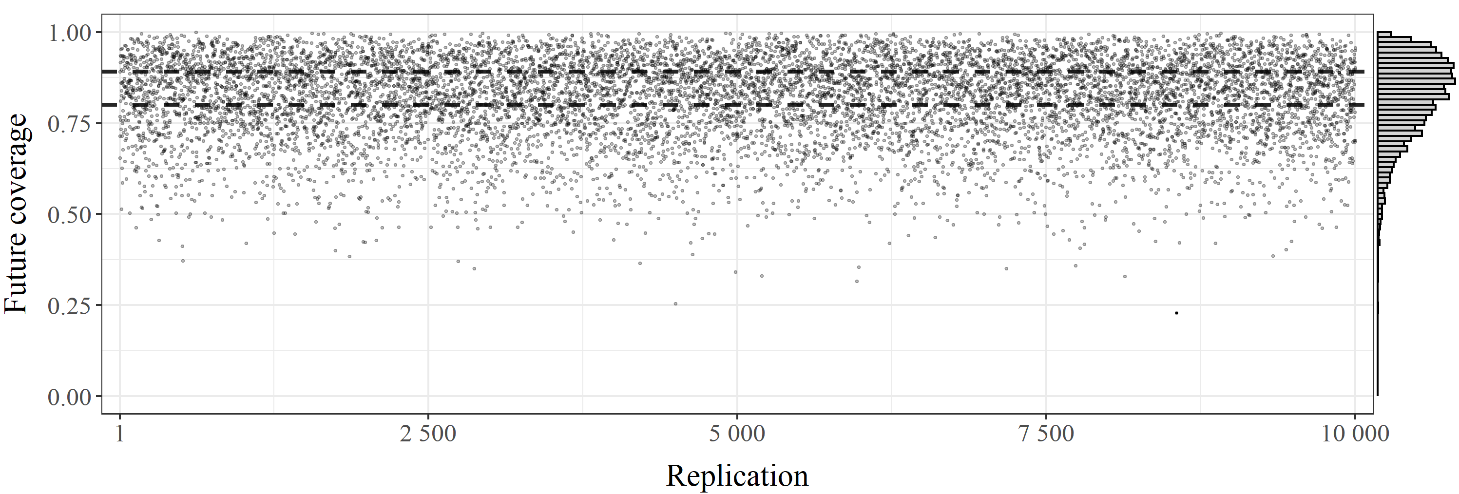
Figure 1: Simulation of the future coverage discussed in Example 5.

Definition 3 seems to imply that to determine the distribution of the future coverage $C^{(n,\alpha)}_{m}$ we would need to model the joint distribution of the indicators $(Z_{1},\dots,Z_{m})$, which are, in general, dependent random variables, due to the way that the random prediction set $D^{(1-\alpha)}_{n}$ introduced in Proposition 2 uses the information contained on the whole training and calibration samples. However, generally it is not possible to model the dependencies between the $Z_{i}$’s without making additional assumptions about the data generating process.

In the next section we show, without imposing additional constraints on the data generating process, how the general nonparametric distribution of the future coverage $C^{(n,\alpha)}_{m}$ is determined as a consequence of the distributional symmetries implied by the fact to be proved in Proposition 3 that the sequence of indicators $\{Z_{i}\}_{i\geq 1}$ is exchangeable under our current assumptions.

3 Coverage distribution

This section presents the two main results of the paper. We begin Section 3.1 establishing that the sequence of indicators $\{Z_{i}\}_{i\geq 1}$ introduced in Definition 3 is exchangeable under our current assumptions. Using this result, a simple symmetry argument connects the marginal validity property with the attributes of the distribution of the future coverage $C^{(n,\alpha)}_{m}$, showing that its expectation $\mathrm{E}[C^{(n,\alpha)}_{m}]$ do satisfy the bounds determined by the marginal validity property in Proposition 2. A connection between the elements that make up the split conformal prediction procedure and Pólya’s urn scheme allows us to determine the exact distribution of the coverage $C^{(n,\alpha)}_{m}$ for a finite horizon of $m$ future observables. In Section 3.2, the exchangeability of the sequence of indicators $\{Z_{i}\}_{i\geq 1}$ and de Finetti’s representation theorem work together to identify the distribution of the almost sure limit of the future coverage $C^{(n,\alpha)}_{m}$ when the horizon $m$ tends to infinity.

3.1 Universal distribution for a finite horizon

Proposition 3.

For exchangeable data, if the conformity scores are almost surely distinct, the sequence of indicators $\{Z_{i}\}_{i\geq 1}$ is exchangeable.

Proof.

Let $k$ be such that $R_{k}$ is the calibration conformity score ranked at the position $\lceil(1-\alpha)(n+1)\rceil$ among the calibration conformity scores $R_{1},\dots,R_{n}$. For $i\geq 1$, we know from Proposition 2 that $Y_{n+i}\in D^{(1-\alpha)}_{n}(X_{n+i})$ if and only if $R_{n+i}<R_{k}$. Define $A=\{t\in\mathbb{R}^{2}:t_{1}<t_{2}\}$ and let $B_{0}=\mathbb{R}^{2}\setminus A$, and $B_{1}=A$. For $z_{1},\dots,z_{m}\in\{0,1\}$, it follows that

$$P\big{(}\cap_{i=1}^{m}\{Z_{i}=z_{i}\}\big{)}=P\big{(}\cap_{i=1}^{m}\{I_{\{R_{n+i}\,<\,R_{k}\}}=z_{i}\}\big{)}=P\big{(}\cap_{i=1}^{m}\{(R_{n+i},R_{k})\in B_{z_{i}}\}.$$

By Proposition 1, the sequence of conformity scores is exchangeable. Therefore, for $i=1,\dots,m$, the random vectors $(R_{n+i},R_{k})$ and $(R_{\pi(n+i)},R_{\pi(k)})$ have the same distribution for every permutation $\pi:\{1,\dots,n+m\}\stackrel{{\scriptstyle\cong}}{{\longrightarrow}}\{1,\dots,n+m\}$. Considering only permutations such that $\pi(j)=j$ for $1\leq j\leq n$, we have that $R_{\pi(k)}=R_{k}$ and

$$P\big{(}\cap_{i=1}^{m}\{Z_{i}=z_{i}\}\big{)} =P\big{(}\cap_{i=1}^{m}\{(R_{\pi(n+i)},R_{k})\in B_{z_{i}}\}\big{)}=P\big{(}\cap_{i=1}^{m}\{I_{\{R_{\pi(n+i)}\,<\,R_{k}\}}=z_{i}\}\big{)}$$

$$=P\big{(}\cap_{i=1}^{m}\{Z_{\pi(i)}=z_{i}\}\big{)}.$$

Since this subclass of permutations is rich enough to express an arbitrary permutation of the indicators $Z_{1},\dots,Z_{m}$, the result follows. ∎

This exchangeability of the sequence $\{Z_{i}\}_{i\geq 1}$ implies that the $Z_{i}$’s are identically distributed, since, for every distinct $i,j\geq 1$, we have $(Z_{i},Z_{j})\sim(Z_{j},Z_{i})$, so that $Z_{i}\sim Z_{j}$. Hence, using Definition 3, by symmetry, $\mathrm{E}[C^{(n,\alpha)}_{m}]=\mathrm{E}[Z_{1}]=P\{Y_{n+1}\in D^{(1-\alpha)}_{n}(X_{n+1})\}$, and $1-\alpha\leq\mathrm{E}[C^{(n,\alpha)}_{m}]\leq 1-\alpha+1/(n+1)$, by Proposition 2.

Therefore, the marginal validity property brings partial information about the distribution of the future coverage, establishing lower and upper bounds for its expectation. In what follows we go beyond this initial characterization, determining the distribution of the future coverage $C^{(n,\alpha)}_{m}$ in full exact form.

Consider the particular case depicted in Figure 2, in which we have a calibration sample of size $n=4$, the nominal miscoverage level $\alpha=0.45$ (so that $\lceil(1-\alpha)(n+1)\rceil=3$), and the horizon $m=5$. Let $b=\lceil(1-\alpha)(n+1)\rceil$ and $g=n-\lceil(1-\alpha)(n+1)\rceil+1$. Since by Proposition 1 the sequence of conformity scores is exchangeable, $R_{5}$ has the same probability of falling into one of the $b+g=n+1=5$ intervals defined by the ordered calibration conformity scores $R_{(1)},\dots,R_{(4)}$ (see the first line in Figure 2). Now, by Definition 3, $Z_{1}=1$ if and only if $R_{5}$ falls into one of the $b=3$ black intervals to the left of $R_{(3)}$ (second line in Figure 2). Hence, $P(Z_{1}=1)=b/(n+1)$. Given that $Z_{1}=1$, $R_{6}$ has, by exchangeability, the same probability of falling into one of the $(b+1)+g=n+2=6$ intervals defined the conformity scores $R_{(1)},\dots,R_{(4)},R_{5}$, and $Z_{2}=0$ if and only if $R_{6}$ falls into one the $g=2$ gray intervals to the right of $R_{(3)}$ (third line in Figure 2). Therefore, $P(Z_{2}=0\mid Z_{1}=1)=g/(n+2)$. Following this reasoning, the product rule yields

$$P(Z_{1}=1,Z_{2}=0,Z_{3}=0,Z_{4}=1,Z_{5}=1)=\frac{b}{n+1}\cdot\frac{g}{n+2}\cdot\frac{g+1}{n+3}\cdot\frac{b+1}{n+4}\cdot\frac{b+2}{n+5},$$

which is manifestly exchangeable, as expected from Proposition 3.

This is a Pólya’s urn scheme [19, 20] with outcome BGGBB in which we started with $b$ black balls (B) and $g$ gray balls (G), and after drawing a ball from the urn we put it back adding one ball of the same color.

The exchangeability of the vector of indicators $(Z_{1},Z_{2},Z_{3},Z_{4},Z_{5})$ implies that the event $\{Z_{1}+Z_{2}+Z_{3}+Z_{4}+Z_{5}=2\}$ is the union of $\binom{m}{2}$ mutually exclusive and equiprobable events of the form $\{Z_{1}=z_{1},Z_{2}=z_{2},Z_{3}=z_{3},Z_{4}=z_{4},Z_{5}=z_{5}\}$, in which $2$ of the $z_{i}$’s are equal to $1$, and $m-2=3$ of the $z_{i}$’s are equal to $0$. Therefore,

$$P(Z_{1}+Z_{2}+Z_{3}+Z_{4}+Z_{5}=2)=\binom{m}{2}\left(\frac{b}{n+1}\cdot\frac{g}{n+2}\cdot\frac{g+1}{n+3}\cdot\frac{b+1}{n+4}\cdot\frac{b+2}{n+5}\right).$$

For real $t$, let $\lfloor t\rfloor$ denote the largest integer smaller than or equal to $t$. Considering that $\lceil-t\rceil=-\lfloor t\rfloor$, and $\lceil k+t\rceil=k+\lceil t\rceil$ for every integer $k$, we can rewrite the initial number of gray balls in the urn as $g=\lfloor\alpha(n+1)\rfloor$.

With the usual convention that an empty product is equal to $1$, a simple induction argument gives the following result.

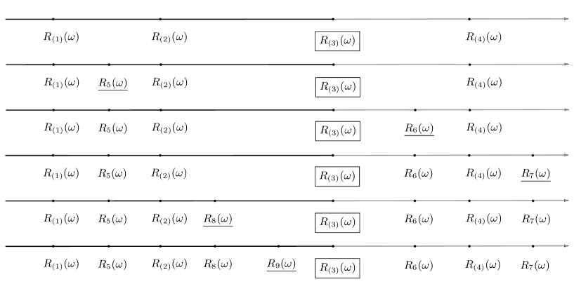
Figure 2: A connection between split conformal prediction and Pólya’s urn scheme.

Theorem 1.

Under the data exchangeability assumption, for every nominal miscoverage level $0<\alpha<1$, every calibration sample size $n\geq 1$, and every horizon $m\geq 1$, if the conformity scores are almost surely distinct, the distribution of the future coverage is given by

$$P(C^{(n,\alpha)}_{m}=k/m)=\binom{m}{k}\frac{\left(\prod_{i=1}^{k}(\lceil(1-\alpha)(n+1)\rceil+i-1)\right)\left(\prod_{i=1}^{m-k}(\lfloor\alpha(n+1)\rfloor+i-1)\right)}{\prod_{i=1}^{m}(n+i)},$$

for $k=1,\dots,m$.

3.2 Almost sure limit

There is a rich literature on exchangeability and its consequences for the foundations of a subjectivistic theory of probability and inference [21, 22, 23, 24, 25, 15, 26]. Here, in the frequentist context of split conformal prediction, we use one of the earliest fundamental results of exchangeability theory as a tool to determine the distribution of the almost sure limit of the future coverage.

For a sequence $\{Z_{i}\}_{i\geq 1}$ of random variables taking values in $\{0,1\}$, de Finetti’s representation theorem [27, 28] states that $\{Z_{i}\}_{i\geq 1}$ is exchangeable if and only if there is a random variable $\Theta:\Omega\to[0,1]$ such that, given that $\Theta=\theta$, the random variables $\{Z_{i}\}_{i\geq 1}$ are conditionally independent and identically distributed with distribution $\text{Bernoulli}(\theta)$. Furthermore, the distribution $\mu_{\Theta}$ of $\Theta$ is unique, and $(1/m)\sum_{i=1}^{m}Z_{i}$ converges almost surely to $\mathbb{E}[Z_{1}\mid\Theta]=\Theta$, when $m$ tends to infinity.

Theorem 2.

For exchangeable data, if the conformity scores are almost surely distinct, the future coverage $C^{(n,\alpha)}_{m}$ converges almost surely when the horizon $m$ tends to infinity to a random variable $C^{(n,\alpha)}_{\infty}$ with distribution $\mathrm{Beta}(\lceil(1-\alpha)(n+1)\rceil,\lfloor\alpha(n+1)\rfloor)$, for every nominal miscoverage level $0<\alpha<1$, and every calibration sample size $n\geq 1$.

Proof.

By Proposition 3, the sequence of indicators $\{Z_{i}\}_{i\geq 1}$ is exchangeable, and de Finetti’s theorem gives us the representation

$$P\{Z_{1}=z_{1},\dots,Z_{m}=z_{m}\}=\int_{[0,1]}\theta^{\sum_{i=1}^{m}z_{i}}(1-\theta)^{m-\sum_{i=1}^{m}z_{i}}\,d\mu_{\Theta}(\theta).$$

For $k=1,\dots,n$, the event $\{\sum_{i=1}^{m}Z_{i}=k\}$ is the union of $\binom{m}{k}$ mutually exclusive and, by exchangeability, equiprobable events of the form $\{Z_{1}=z_{1},\dots,Z_{m}=z_{m}\}$, in which $k$ of the $z_{i}$’s are equal to $1$, and $m-k$ of the $z_{i}$’s are equal to $0$. Therefore, it follows from the integral representation above that

$$P(C^{(n,\alpha)}_{m}=k/m)=P\!\left({\textstyle\sum_{i=1}^{m}Z_{i}=k}\right)=\binom{m}{k}\int_{[0,1]}\theta^{k}(1-\theta)^{m-k}\,d\mu_{\Theta}(\theta).$$

Let $\mu_{\Theta}$ be dominated by Lebesgue measure $\lambda$ with Radon-Nikodym derivative

$$(d\mu_{\Theta}/d\lambda)(\theta)=\left(\frac{n!}{(b-1)!(g-1)!}\right)\theta^{b-1}(1-\theta)^{g-1}\,I_{[0,1]}(\theta),$$

up to almost everywhere $[\lambda]$ equivalence, in which $b=\lceil(1-\alpha)(n+1)\rceil$ and $g=\lfloor\alpha(n+1)\rfloor$. This is a version of the density of a random variable with $\mathrm{Beta}(b,g)$ distribution. Using the Leibniz rule for Radon-Nikodym derivatives (see [15], Theorem A.79), we have that

$$P(C^{(n,\alpha)}_{m}=k/m) =\binom{m}{k}\left(\frac{n!}{(b-1)!(g-1)!}\right)\int_{[0,1]}\theta^{k+b-1}(1-\theta)^{m-k+g-1}\,d\lambda(\theta)$$

$$=\binom{m}{k}\left(\frac{n!}{(b-1)!(g-1)!}\right)\left(\frac{(k+b-1)!(m-k+g-1)!}{(m+n)!}\right)$$

$$=\binom{m}{k}\frac{\left(\prod_{i=1}^{k}(b+i-1)\right)\left(\prod_{i=1}^{m-k}(g+i-1)\right)}{\prod_{i=1}^{m}(n+i)}.$$

Since de Finetti’s theorem states that $\mu_{\Theta}$ is unique and that $C^{(n,\alpha)}_{m}$ converges almost surely to $\Theta$, when $m$ tends to infinity, the result follows by inspection of the distribution of the future coverage $C^{(n,\alpha)}_{m}$ in Theorem 1. ∎

As corollaries, we note that the usual properties of the beta distribution yield

$$\mathrm{E}[C^{(n,\alpha)}_{\infty}]=\frac{\lceil(1-\alpha)(n+1)\rceil}{n+1}=1-\alpha+O\!\left(\frac{1}{n}\right);$$

$$\mathrm{Var}[C^{(n,\alpha)}_{\infty}]=\frac{\lceil(1-\alpha)(n+1)\rceil\times\lfloor\alpha(n+1)\rfloor}{(n+1)^{2}(n+2)}=\frac{\alpha(1-\alpha)}{n}+O\!\left(\frac{1}{n^{2}}\right).$$

Furthermore, using the expression of the beta density, a simple application of Scheffé’s theorem [29] tells us that

$$\sqrt{n}(C^{(n,\alpha)}_{\infty}-(1-\alpha))\xrightarrow[n\to\infty]{d}\mathrm{N}(0,\alpha(1-\alpha)).$$

4 Concluding remarks

For a nominal miscoverage level $0<\alpha<1$, we may want to choose the calibration sample size $n$ in order to control the distribution of $C^{(n,\alpha)}_{\infty}$. Define the cumulative distribution function $H_{n,\alpha}(t)=P(C^{(n,\alpha)}_{\infty}\leq t)$, for $t\in\mathbb{R}$. Fixing some $\epsilon>0$ and $0<\gamma<1$, the calibration sample size can be chosen as $\min\,\{n\geq 1:H_{n,\alpha}(1-\alpha+\epsilon)-H_{n,\alpha}(1-\alpha-\epsilon)\geq\gamma\}$. For instance, with $1-\alpha=0.9$, $\epsilon=0.02$, and $\gamma=0.95$, using this criterion, we get a calibration sample size $n=860$.

References

- [1] V. Vovk, A. Gammerman, and C. Saunders, “Machine-learning applications of algorithmic randomness,” in Proceedings of the Sixteenth International Conference on Machine Learning, ICML ’99, (San Francisco, CA, USA), pp. 444–453, Morgan Kaufmann Publishers Inc., 1999.
- [2] H. Papadopoulos, K. Proedrou, V. Vovk, and A. Gammerman, “Inductive confidence machines for regression,” in Machine Learning: ECML 2002 (T. Elomaa, H. Mannila, and H. Toivonen, eds.), (Berlin, Heidelberg), pp. 345–356, Springer Berlin Heidelberg, 2002.
- [3] V. Vovk, A. Gammerman, and G. Shafer, Algorithmic learning in a random world. Springer Science & Business Media, 2005.
- [4] G. Shafer and V. Vovk, “A tutorial on conformal prediction,” Journal of Machine Learning Research, vol. 9, no. 12, pp. 371–421, 2008.
- [5] J. Lei, M. G’Sell, A. Rinaldo, R. J. Tibshirani, and L. Wasserman, “Distribution-free predictive inference for regression,” Journal of the American Statistical Association, vol. 113, no. 523, pp. 1094–1111, 2018.
- [6] M. Fontana, G. Zeni, and S. Vantini, “Conformal prediction: A unified review of theory and new challenges,” Bernoulli, vol. 29, no. 1, pp. 1–23, 2023.
- [7] T. Hastie, R. Tibshirani, and J. Friedman, The Elements of Statistical Learning: Data Mining, Inference, and Prediction. Springer, 2nd ed., 2009.
- [8] K. P. Murphy, Machine Learning: A Probabilistic Perspective. MIT Press, 2012.
- [9] C. M. Bishop, Pattern Recognition and Machine Learning. Springer, 2006.
- [10] I. J. Goodfellow, Y. Bengio, and A. Courville, Deep Learning. Cambridge, MA, USA: MIT Press, 2016.
- [11] Y. Romano, E. Patterson, and E. Candès, “Conformalized quantile regression,” in Advances in Neural Information Processing Systems (H. Wallach, H. Larochelle, A. Beygelzimer, F. d'Alché-Buc, E. Fox, and R. Garnett, eds.), vol. 32, Curran Associates, Inc., 2019.
- [12] L. Breiman, “Random Forests,” Machine Learning, vol. 45, no. 1, pp. 5–32, 2001.
- [13] J. H. Friedman, “Greedy function approximation: A gradient boosting machine,” Annals of Statistics, vol. 29, pp. 1189–1232, 2001.
- [14] N. Meinshausen, “Quantile regression forests,” Journal of Machine Learning Research, vol. 7, no. 35, pp. 983–999, 2006.
- [15] M. J. Schervish, Theory of statistics. Springer Series in Statistics, 1995.
- [16] J. Lei and L. Wasserman, “Distribution-free prediction bands for non-parametric regression,” Journal of the Royal Statistical Society: Series B: Statistical Methodology, pp. 71–96, 2014.
- [17] R Core Team, R: a language and environment for statistical computing. R Foundation for Statistical Computing, Vienna, Austria, 2017.
- [18] J. H. Friedman, “Multivariate Adaptive Regression Splines,” The Annals of Statistics, vol. 19, no. 1, pp. 1–67, 1991.
- [19] F. Eggenberger and G. Pólya, “Über die statistik verketteter vorgänge,” Zeitschrift für Angewandte Mathematik und Mechanik, vol. 3, no. 4, pp. 279–289, 1923.
- [20] W. Feller, An Introduction to Probability Theory and Its Applications, vol. 1. Wiley, 1968.
- [21] B. de Finetti, Theory of Probability: A Critical Introductory Treatment. Wiley, 1979.
- [22] E. S. Hewitt and L. J. Savage, “Symmetric measures on cartesian products,” Transactions of the American Mathematical Society, vol. 80, pp. 470–501, 1955.
- [23] J. F. C. Kingman, “Uses of Exchangeability,” The Annals of Probability, vol. 6, no. 2, pp. 183 – 197, 1978.
- [24] D. Aldous, “Exchangeability and related topics,” in École d’été de probabilités de Saint-Flour, XIII—1983, pp. 1–198, Springer, 1985.
- [25] S. Wechsler, “Exchangeability and predictivism,” Erkenntnis, vol. 38, no. 3, pp. 343–350, 1993.
- [26] O. Kallenberg, Probabilistic symmetries and invariance principles. Springer, 2005.
- [27] B. de Finetti, “Funzione caratteristica di un fenomeno aleatorio,” Atti della R. Accademia Nazionale dei Lincei, Ser. 6. Memorie, Classe di Scienze Fisiche, Matematiche e Naturali 4, pp. 251–299, 1931.
- [28] B. de Finetti, “La prévision: Ses lois logiques, ses sources subjectives,” Annales de l’Institut Henri Poincaré, vol. 17, pp. 1–68, 1937.
- [29] H. Scheffé, “A Useful Convergence Theorem for Probability Distributions,” The Annals of Mathematical Statistics, vol. 18, no. 3, pp. 434–438, 1947.