Resonant two-laser spin-state spectroscopy of a negatively charged quantum dot-microcavity system with a cold permanent magnet

Abstract

A high-efficiency spin-photon interface is an essential piece of quantum hardware necessary for various quantum technologies. Self-assembled InGaAs quantum dots have excellent optical properties, if embedded into an optical micro-cavity they can show near-deterministic spin-photon entanglement and spin readout, but an external magnetic field is required to address the individual spin states, which usually is done using a superconducting magnet. Here, we show a compact cryogenically compatible SmCo magnet design that delivers $475\,\mathrm{\textrm{mT}}$ in-plane Voigt geometry magnetic field at $5\,\mathrm{\textrm{K}}$, which is suitable to lift the energy degeneracy of the electron spin states and trion transitions of a single InGaAs quantum dot. This quantum dot is embedded in a birefringent high-finesse optical micro-cavity which enables efficient collection of single photons emitted by the quantum dot. We demonstrate spin-state manipulation by addressing the trion transitions with a single and two laser fields. The experimental data agrees well to our model which covers single- and two-laser cross-polarized resonance fluorescence, Purcell enhancement in a birefringent cavity, and variation of the laser powers.

I introduction

An efficient, tunable spin-photon interface that allows high fidelity entanglement of spin qubits with flying qubits, photons, lies at the heart of many building blocks of distributed quantum technologies Awschalom2018 , ranging from quantum repeaters Kimble2008 , photonic gates Koshino2010 ; Rosenblum2011 , to the generation of photonic cluster states Lindner2009 ; Schwartz2016 ; Coste2022 . Further, to secure connectivity within the quantum network, an ideal spin-photon interface requires near-unity collection efficiency, therefore an atom or semiconductor quantum dot (QD) carrying a single spin as a quantum memory is integrated into photonic structures such as optical microcavities cavities, where recently $57\,\%$ in-fiber photon collection efficiency has been achieved Tomm2021 .

Within the pool of promising systems, singly-charged excitonic complexes of optically active QD devices in III-V materials Warburton2013 combines near-unity quantum efficiency, excellent zero-phonon line emission at cryogenic temperatures Favero2003 with nearly lifetime-limited optical linewidth Kuhlmann2015 . This, in combination with sub-nanosecond Purcell-enhanced lifetimes, enabled GHz-scale generation rates of indistinguishable single-photons Santori2002 ; He2013 ; Ding2016 ; Somaschi2016 ; Senellart2017 ; Hilaire2020 ; Tomm2021 , robust polarization selection rules Bayer2002 ; Stockill2017 , and simple on-chip integration facilitating stable-long term operation and tuneability.

The singly-charged quantum dot can be optically excited to the trion state, if this is done with linearly polarized light, the spin state of the resident electron is transferred to the trion hole spin by the optical selection rules. If the trion decays, it will emit a single circularly polarized photon with a helicity depending on the hole spin state, Fig. 1(a). To achieve selective spin addressability which is necessary for spin initialization and readout, the QD is typically placed in an external in-plane (Voigt geometry) magnetic field Emary2007 ; Xu2007 , which induces Zeeman splitting of the spin states and trion transitions Bayer2002 . The magnetic field modifies the eigenstates of the system and the optical selection rules, and four optical transitions are possible (see Fig. 1(b)), which are now linearly polarized. The electron and trion spin, as well as the photon polarization, are now connected by the modified optical selection rules. We obtain two intertwined $\Lambda$ systems which can be used with steady-state light fields for spin initialization Xu2007 ; Emary2007 , arbitrary spin ground state superposition generation Xu2008 , or dynamical spin decoupling from the nuclear bath Xu2009 .

This spin manipulation gets harder if the quantum dot is placed in a non-polarization degenerate (birefringent) micro-cavity Tomm2021 ; Steindl2021_PRL ; Hilaire2020 . Here we show two-laser resonant spectroscopy Xu2007 ; Kroner2008PRB of a single spin in a single quantum dot in such a birefringent cavity, and use cross-polarized collection of single photons. We use a simple “set-and-forget” cryogenic permanent magnet assembly to apply the magnetic field, and we are able to derive the spin dynamics by comparison to a theoretical model.

II Permanent magnet assembly

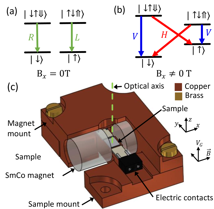
Figure 1: Energy level schemes of negatively charged QD and magnetic assembly. Optical selection rules of trion transitions without (a) and with (b) an external in-plane magnetic field. (c) Schematic of the permanent magnet assembly.

Magneto-optical quantum dot-based experiments usually rely on large and complex superconducting magnets Coste2022 ; Huber2019 , which generate strong magnetic fields but require both a stabilized current source and cryogenic temperatures. However, many experiments need only a “set-and-forget” static magnetic field of around $500\,\mathrm{mT},$ which can be achieved with compact strong permanent magnets cooled down together with the quantum dot device Androvitsaneas2016 ; Androvitsaneas2019 ; Adambukulam2021 . Unfortunately, many rare-earth magnetic materials such as NdFeB Fredricksen2003 suffer at cryogenic temperatures from spin reorientation Tokuhara1985 which lowers the effective magnetic field He2013_magnet and tilts the easy axis of the magnetic assembly Hara2004 ; Fredricksen2003 . Especially, losing control over the magnetic field direction is problematic with quantum dots since it affects mixing between dark and bright states and thus changes both transition energies and optical selection rules Bayer2000 .

To build our permanent magnet assembly, we have chosen from the strongest commercially available magnetic materials Miyake2018 ; Wang2021 SmCo (grade 2:17) magnets with a room temperature remanence of $1.03\,\mathrm{T}$. This industrially used magnetic system is known for its high Curie temperature (over $800\,^{\circ}\mathrm{C}$) and high magnetocrystalline anisotropy Zhou2000 ; Gutfleisch2000 excellent for high-temperature applications in several fields Gutfleisch2011 ; Duerrschnabel2017 ; Guo2022 . Especially it is used above the Curie temperatures of NdFeB of $310\,^{\circ}\mathrm{C}$ Gutfleisch2000 , where current NdFeB-based magnets have relatively poor intrinsic magnetic properties. Moreover, due to low temperature-dependence of remanence and coercivity Durst1986 ; Liu2019 ; Wang2021 , SmCo-based magnets also show excellent thermal stability of the remanence with near-linear dependence Durst1986 ; He2013_magnet down to $4.2\,\mathrm{K}$. This is in contrast to other common rare-earth magnet compounds such as NdFeB Fredricksen2003 , where the remanence at temperatures below $135\,\mathrm{K}$, depending on the specific material composition He2013_magnet , decreases rapidly by several percent due to the spin-reorientation transition Tokuhara1985 .

Our permanent magnet assembly in Fig. 1(c) is designed to fit on top of a $XYZ$ piezo motor assembly in a standard closed-cycle cryostat with optical access via an ambient-temperature long working distance objective, which restricts its physical dimensions to approximately $1\,\mathrm{cm}$ in height. Thus, we built the assembly from two $9\times 9\,\mathrm{mm}$ commercially available rod-shaped SmCo magnets separated by a $4.5\,\mathrm{\textrm{mm}}$ air gap embedded in a $36\times 24\times 10.8\,\mathrm{mm}$ copper housing. Due to the large remanence ($1.03\,\mathrm{T}$) and small air gap, the assembly in the center of the gap produces a homogeneous magnetic field of about $500\,\mathrm{\textrm{mT}}$, as discussed in Appendix A. The assembly is rigidly attached by brass screws to the H-shaped copper sample mount, where the quantum dot device is horizontally placed in the center of the air gap such that the magnetic field is in-plane (Voigt geometry). The assembly contains electrical contacts to apply a bias voltage $V_{\textrm{G}}$ to the device. It has a low weight of $69\,\mathrm{\textrm{g}}$ (including $4.8\,\mathrm{g}$ per magnet), compatible with standard nanopositioners allowing for fine-tuning of the sample position with respect to the optical axis.

The magnetic mount is then cooled down together with the sample to approximately $5\,\mathrm{K}.$ Since in SmCo, the spin reorientation transition was reported to be stable down to $10\,\mathrm{K}$ He2013_magnet , we do not expect magnetization axis changes and assume only a small magnetic field drop of $5\,\%$ between the room and cryogenic temperatures Fredricksen2003 . This makes SmCo an ideal material choice for strong homogeneous cryogenic magnets, in our case delivering about $475\,\mathrm{mT}$ at $5\,\mathrm{K}$.

III Spin-state determination

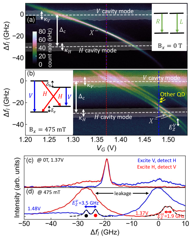
Figure 2: Resonant reflection as a function of laser frequency and gate voltage without (a) and with (b) an in-plane external magnetic field, plotted with the same color scale. The excitation laser is polarized along the $V$ cavity axis and reflected laser light is filtered out using a crossed $H$ polarizer, to select photons emitted by the QD trion. Insets show the corresponding optical selection rules. Dashed lines indicate the cavity resonance frequencies with the cavity decay rates $\kappa_{V}$, $\kappa_{H}$, determined using semi-classical model fits Snijders2020 . Panels (c, d) show cross-sectional plots without and with magnetic field for two excitation polarizations (blue: excitation along $V$ cavity mode, red: $H$) at voltages $1.37\,\mathrm{V}$ or $1.48\,\mathrm{V}$, indicated by the vertical lines in panels (a, b). The Zeeman splittings determined from Lorentzian fits (black dashed lines) are given. The excitation power in front of excitation objective is $2\,\mathrm{nW}$, laser scanning speed $41\,\mathrm{GHz}\mathrm{/s}$.

We study self-assembled InGaAs quantum dots emitting around $\lambda=935.5\,\mathrm{nm}$, embedded in $\sim\lambda$ thick GaAs planar cavity, surrounded by two distributed Bragg reflectors (DBR): 26 pairs of $\lambda/4$ thick GaAs/A$\text{l}_{0.90}$G$\text{a}_{0.10}$As layers from the top and 13 pairs of GaAs/AlAs layers and 16 pairs of GaAs/A$\text{l}_{0.90}$G$\text{a}_{0.10}$As layers at the bottom Snijders2018 ; Steindl2021_PRL . The single QD layer is embedded in a p-i-n junction, separated from the electron reservoir by a $31.8\,\mathrm{nm}$ thick tunnel barrier including a $21.8\,\mathrm{nm}$ thick A$\text{l}_{0.45}$G$\text{a}_{0.55}$As electron blocking layer designed to allow single electron charging of the QD Heiss2008 ; Heiss2010 . A voltage bias $V_{\textrm{G}}$ applied over the diode allows for charge-control of the ground state of the quantum dot and also to fine-tune the QD transition energies into resonance with the optical cavity mode. The optical in-plane cavity mode confinement is achieved by an oxide aperture, we fabricate 216 cavities per device Frey_phdthesis and select a suitable one with (i) a quantum dot well-coupled to the cavity mode and (ii) low birefringence of the fundamental mode, for the device studied here, the two linearly-polarized modes cavity modes ($H$ and $V$ modes) are split by $\Delta_{\textrm{c}}=28\,\mathrm{GHz}$.

First, we cool down the device to 5 K without the SmCo magnet assembly in a closed-cycle cryostat. For resonant laser spectroscopy, we use a cross-polarization laser extinction method with laser rejection better than $10^{6}$ Steindl2023_PER . Using a free-space polarizer and half-waveplate, the polarization of the excitation laser is aligned along the $V$ cavity polarization axis, and the light reflected from the cavity is recorded with a single-photon detector after passing again the half-wave plate and the crossed polarizer. In Fig. 2(a), we show a fluorescence map of this device measured in the cross-polarization scheme as a function of the laser frequency detuning from the $V$-polarized cavity mode resonance $\Delta f_{l}$ and applied bias voltage $V_{\textrm{G}}$. We observe a single emission line which is shifted by the quantum-confined Stark effect, the line is in resonance with the $V$ cavity mode at around $1.25\,\mathrm{V}$ and with the $H$ cavity mode at around $1.40\,\mathrm{V}$. The same line is visible also if the excitation and detection polarization are swapped, see the cross-sectional plot in Fig. 2(c). The fact that we observe the same single line under both perpendicular polarizations and that it is coupled to both fundamental cavity modes, suggests that the emitted photons are circularly polarized and originate from the charged exciton $X^{-}$.

Now we cool down the device with the SmCo magnet assembly, to lift the energy degeneracy of the trion transitions. In this scenario, with the energy level scheme in Fig. 2(b), the optical selection rules are modified by the in-plane magnetic field from circular to linear polarization. Thus the scanning excitation laser polarized along the $V$ cavity mode can only resonantly address $V$-polarized transitions, i.e., $\left|\downarrow\right\rangle\rightarrow\left|\downarrow\uparrow\Downarrow\right\rangle$ and $\left|\uparrow\right\rangle\rightarrow\left|\uparrow\downarrow\Uparrow\right\rangle$, therefore we expect to observe a pair of lines Zeeman-split by the energy $E_{\textrm{Z}}^{V}=\delta_{\textrm{e}}+\delta_{\textrm{h}}$. Without cavity enhancement, each of the excited trion states radiatively decays with equal probability (by cavity Purcell enhancement, however, this is modified) into the single-spin ground state by emission of a single photon with either $V$ or $H$ polarization depending on the excited and ground states, as depicted in Fig. 2(b). Because we measure in cross-polarization, we filter out the emitted $V$-polarized single photons and detect only photons emitted by the $\left|\downarrow\uparrow\Downarrow\right\rangle\rightarrow\left|\uparrow\right\rangle$ and $\left|\uparrow\downarrow\Uparrow\right\rangle\rightarrow\left|\downarrow\right\rangle$ transitions. Thus, the total detected rate is reduced to half of that without magnetic field. Similarly, the scanning laser polarized along the $H$ cavity mode excites only $\left|\uparrow\right\rangle\rightarrow\left|\downarrow\uparrow\Downarrow\right\rangle$ and $\left|\downarrow\right\rangle\rightarrow\left|\uparrow\downarrow\Uparrow\right\rangle$, and we observe again a pair of fluorescence lines, this time Zeeman split by $E_{\textrm{Z}}^{H}=|\delta_{\textrm{e}}-\delta_{\textrm{h}}|$. Note that in Fig. 2(b) we observe two pairs of emission lines which originate from two different QDs. We focus only on the brighter QD, corresponding to the clear transition in Fig. 2(a). In agreement with the trion energy level scheme, the trion transitions exhibit a different Zeeman splitting of $E_{\textrm{Z}}^{V}=3.5\pm 0.1\,\mathrm{GH\mathrm{z}}$ under $V$- and $E_{\textrm{Z}}^{H}=1.9\pm 0.1\,\mathrm{GHz}$ $H$-polarization excitation. This Zeeman splitting was extracted by Lorentizan fits to laser frequency scans shown in Fig. 2(d), which allows us to estimate Bennett2013 the electron and hole g-factors, we obtain $|g_{\textrm{e}}|=0.39$ and $|g_{\textrm{h}}|=0.12$; these values agree to literature values for small InGaAs QDs Nakaoka2004 . We also observe a $25\,\textrm{GHz}$ energy average shift of the QD emission caused by a combination of the diamagnetic shift (around $0.5\,\textrm{GHz}$ assuming diamagnetic constant $-9.4\,\textrm{$\mu$eV/$T^{2}$}$ Kroner2008PRB ), and temperature/strain induced band-gap changes between consecutive cooldowns. Note that we also observe a broad emission, which is most likely due to cavity-enhanced fluorescence in combination with imperfect polarization alignment and due to our limited cross-polarization extinction ratio of $4\times 10^{6}$ Steindl2023_PER .

IV Two-color resonant laser excitation

Now, we demonstrate spin-state manipulation using two individually tunable narrow-linewidth lasers. For a high-degree cross-polarization extinction ratio, we perform resonance fluorescence spectroscopy in the vicinity of the $H$-cavity mode ($V_{\textrm{G}}=1.49\,\mathrm{V}$, i.e., we focus on the transitions marked by dots in Fig. 2(d)), and we use $V$ polarization of both excitation lasers. In Fig. 3(d), we show a reflection map measured in cross-polarization as a function of both laser frequencies $f_{l}$ (pump) and $f_{r}$ (repump). The horizontal and vertical lines indicate the trion transition frequencies. Where these frequencies intersect interesting dynamics occurs. First, the nodes oriented along the diagonal represent a condition where both lasers are resonant with the same transition corresponding to the excitation scheme depicted in Fig. 3(b). We will call this configuration two-laser resonant excitation (2LRE). The system dynamics under this excitation is equivalent to single-laser excitation (1LRE) with stronger emission due to the higher driving power of $P_{l}+P_{r}$. The anti-diagonally oriented nodes correspond to emission under two-color excitation where each laser pumps a distinct transition [Fig. 3(c)]; we refer to this scheme as two-color resonant excitation (2CRE) Kroner2008PRB . For clarity, we further focus only on the situation where the first laser of constant power $P_{l}$ continuously pumps the $\left|\downarrow\right\rangle\rightarrow\left|\downarrow\uparrow\Downarrow\right\rangle$ transition. Due to cross-polarization detection, we observe only $H$-polarized emission from the $\left|\downarrow\uparrow\Downarrow\right\rangle\rightarrow\left|\uparrow\right\rangle$ transition, a signature of population shelving into the $\left|\downarrow\right\rangle$ spin state. This shelved population is repumped, and thus, the total (detected) single-photon rate increased by re-pumping the $\left|\uparrow\right\rangle\rightarrow\left|\uparrow\downarrow\Uparrow\right\rangle$ transition with the second laser, and we observe a higher photon rate at the anti-diagonal nodes in Fig. 3(d).

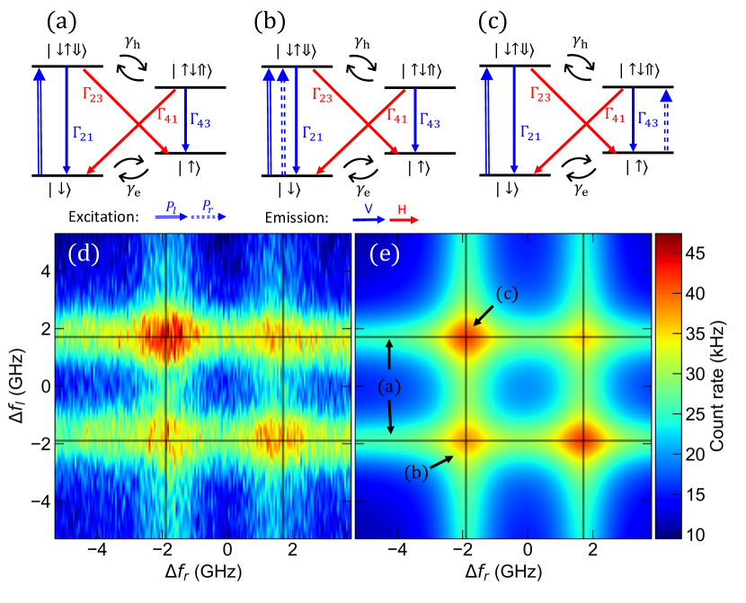
Figure 3: Two-color laser trion spectroscopy with a magnetic field in Voigt geometry. (a-c) Comparison of three different trion excitation conditions: single-laser excitation (a), two same-frequency lasers (b), and (c) each laser addresses different trion transitions. Experiment (d) and model (e) data for of two-color experiments, for $P_{l}=2.1\>\mathrm{nW}$ pump laser power and $P_{r}=2.0\,\mathrm{nW}$ repump laser power, the black lines indicate the QD trion transition frequencies.

To gain a more precise knowledge of the magnitude of the spontaneous decay rates $\Gamma_{xy}$ as well as electron and hole spin-flip rates $\gamma_{\textrm{e}}$ and $\gamma_{\textrm{h}}$ involved in the system dynamics, we compare our experiments to a model which is derived in the Appendix D. For a laser power below the saturation power $P_{\textrm{c}}$, the model is derived from the rate equations describing the steady-state two-scanning lasers pump of the trion energy scheme in Fig. 3. The trion transitions are modeled as two coupled $\Lambda$ systems with asymmetric $V$ and $H$-polarized radiative transition rates due to cavity enhancement of the latter. A careful analysis of the model parameters and comparison to our experimental results allows us to determine the electron spin-flip rates to be $\gamma_{\textrm{e}}\approx 2.5\,\mathrm{MHz}$, while the hole spin-flip rate cannot be determined because of the short lifetime of the excited trion states, as expected. Further we obtain lifetimes of $\Gamma_{21}=2.1\,\textrm{GHz},\Gamma_{43}=2.7\mathrm{\,GHz}$, and $\Gamma_{23}=\Gamma_{41}=0.8\,\mathrm{GHz}$. Similar spin-flip rates were reported in earlier resonant two-color trion spectroscopy without cavity Kroner2008PRB ; the cavity-enhanced radiative rates $\Gamma_{21}$, $\Gamma_{43}$ agree with our power-broadening analysis, see Appendix C.

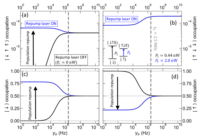
Figure 4: Steady-state trion states (a, b) and electron ground-state spin (c, d) occupation probability as a function of electron spin-flip rate, with (blue) and without (blue) repump laser. The dashed lines show the determined spin-flip rate of $\gamma_{\textrm{e}}\approx 2.5\,\mathrm{MHz}$.

Figure 4 shows spin-flip rate dependency of the steady state occupation of the trion and electron spin states predicted by our theory. In the simulation with varied $\gamma_{\textrm{e}}$, we used system parameters found above together with laser powers $P_{l}=0.44\,\textrm{nW}$ and $P_{r}=2.0\,\textrm{nW}$ to demonstrate spin pumping. First, if the electron spin-flip rate is small (below $1\,\textrm{kHz}$), the weak pump laser light initializes the spin state $\left|\uparrow\right\rangle$. By optical repumping with the second laser on resonance with $\left|\uparrow\right\rangle\rightarrow\left|\uparrow\downarrow\Uparrow\right\rangle$, the shelved spin population can be largely transferred from $\left|\uparrow\right\rangle$ into $\left|\downarrow\right\rangle$ as demonstrated in Fig. 4(c,d). Due to the optical repumping, the resonant absorption on spin $\left|\uparrow\right\rangle$ becomes again possible, leading experimentally in the recovery of transmission signal at the resonant frequency with $\left|\downarrow\right\rangle\rightarrow\left|\downarrow\uparrow\Downarrow\right\rangle$ Kroner2008PRB ; Atature2006 . Our simulation for the determined spin-flip rate of $\gamma_{\textrm{e}}\approx 2.5\,\mathrm{MHz}$ shows that the electron spin-flip leads to a comparable spin population of both ground states even without repumping laser field, making conclusive absorption measurements difficult because of the small change between ground state populations with and without optical repumping. However, the spin repumping from $\left|\uparrow\right\rangle$ is accompanied by the population of $\left|\uparrow\downarrow\Uparrow\right\rangle$ resulting in extra emission from this spin state. Importantly, the presence of this extra emission is independent of the ground state spin-flip rate and can be thus used as a signature of optical spin repumping. Moreover, at low $\gamma_{\textrm{e}}$, the emission following the spin repumping benefits also from the extra excited state population of the state $\left|\downarrow\uparrow\Downarrow\right\rangle$, see Fig. 4(a).

Finally, we test our model against a series of excitation-power-dependent experiments shown in Fig. 5. Both observed trion transitions under 1LRE (black and red symbols corresponding to lines in Fig. 2(d)) show saturation with power described by $180\,\mathrm{kHz}/(1+P_{\textrm{c}}/P)$ loudon_quantum_1973 ; Snijders2018 with a reasonable saturation power of $P_{\textrm{c}}=22\pm 2\,\mathrm{nW}$, in agreement to our model.

In contrast to these single-frequency measurements, the 2CRE scheme shown by the blue symbols in Fig. 5 shows clear signs of spin repumping: Due to the continuous repumping of the spin population of both ground states with the two lasers (at a constant $P_{r}=2.0\,\mathrm{nW}$), we control the individual steady-state spin populations by altering the relative power of the lasers. Because higher repumping power leads to stronger repumping and thus to higher excited-state occupation, we experimentally observe increased photon rates, following our model predictions. This increase varies with relative powers between pump and repump laser beam from a factor higher than 10 at $P_{l}=0.44\,\textrm{nW}$ to factor $1.3$ above $P_{\textrm{c}}$.

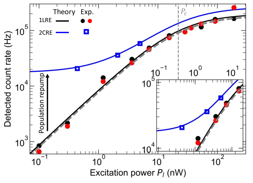
Figure 5: Power dependency of the trion resonant fluorescence under different excitation schemes, comparing experimental photon count rates (symbols) to our model (lines) with $\gamma_{\textrm{e}}=2.5\,\textrm{MHz}$: Only pump laser for both trion transition (1LRE, black and red) and with repump laser (2CRE, blue). The gray dashed lines indicate the standard two-level system saturation behaviour.

V Conclusions

We developed a compact cryogenic SmCo permanent magnet assembly delivering an in-plane magnetic field of $475\,\mathrm{mT}$. In contrast to superconducting solenoids, this solution does not need any active control and works from cryogenic to ambient temperatures. Therefore, we believe it could become a preferable, economical, and scalable architecture for spin-photon interfaces where the magnetic field is used in “set-and-forget” mode.

Using this magnetic assembly in Voigt geometry, we have shown Zeeman splitting and spin addressability of the electron and trion states of a negatively charged quantum dot embedded in a birefringent optical microcavity. We demonstrate spin-state manipulation using continuous-wave resonant two-laser spectroscopy, which in combination with a high-extinction ratio cross-polarization technique enables background-free single-photon readout. This two-laser excitation scheme, similar to earlier schemes Xu2007 ; Xu2008 ; Kroner2008PRB without a cavity, will allow for spin-state initialization and manipulation.

Appendix A Permanent magnet assembly simulations

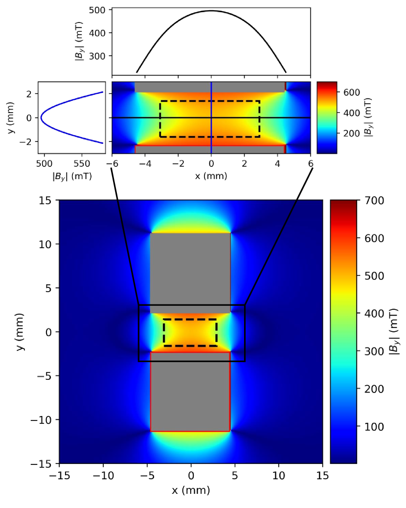
Figure A1: Magnetic field simulation of the magnetic assembly with a $4.5\,\mathrm{mm}$ air gap at room temperature. The magnitude of the magnetic field strength $|B_{y}|$ along an $xy$-cross-section of the assembly (grey regions), with the location of the sample taken to be the origin (outlined by the dashed line). (Inset) Zoom-in $|B_{y}|$ to the sample region with cross-sections along the $x$ (top) and $y$ (left) direction through the center of the sample.

The magnetic assembly was simulated using Magpylib – a Python package for magnetic field computation magpylib2020 . Given the large and thermally stable coercivity of SmCo magnets at cryogenic temperatures Liu2019 ; Wang2021 , we model the permanent magnets as $9\times 9\>\mathrm{mm}$ large rods insensitive to any external magnetic field with a residual magnetization of $1.03\,\mathrm{T}$. The copper housing of the magnet was not included in the simulations, because copper is a weak magnetic metal with low magnetic susceptibility Bowers1956 . The room temperature simulation of our magnetic mount with a $4.5\,\mathrm{mm}$ air gap between the magnetic rods is presented in Fig. A1. From the simulation, we see that the assembly produces a strong magnetic field (beyond $500\,\mathrm{mT}$) confined between the poles of the magnets. Due to the simple assembly design, the magnetic field is inhomogeneous over the entire sample footprint of several square millimeters. However, over the few nanometer-size quantum dot used later in the experiments, the magnetic field can be assumed homogenous. In our experiments, we use QD close to the coordinate origin in Fig. A1, where the external magnetic field reaches a strength of $500\,\mathrm{mT}$.

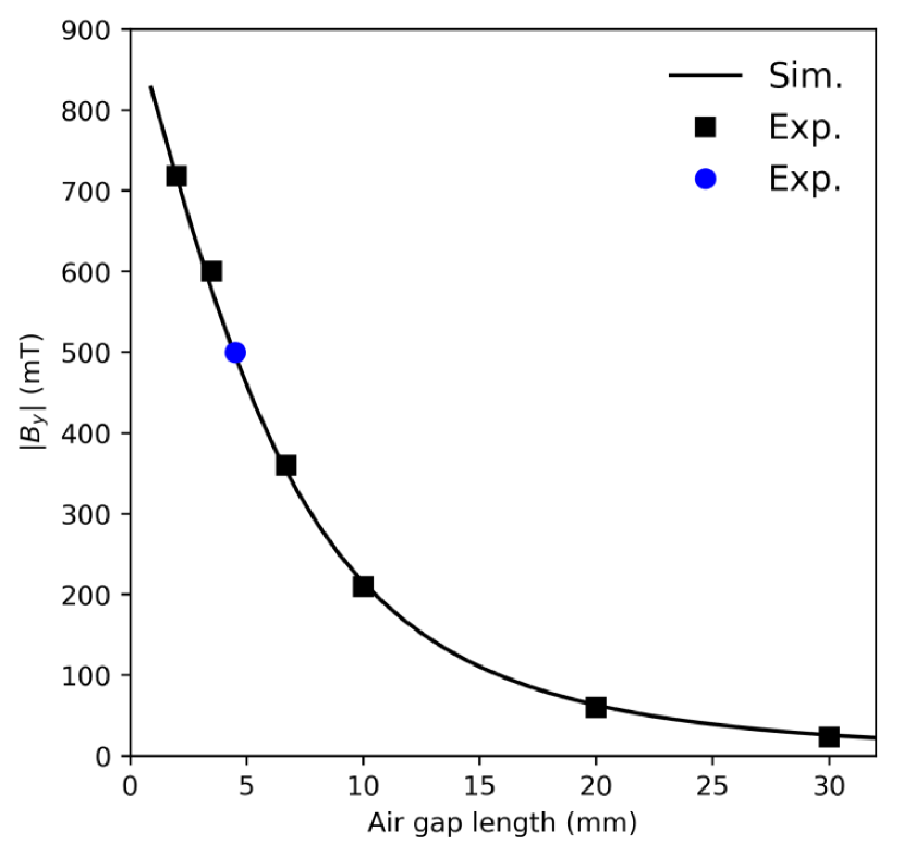
Figure A2: Air gap length dependence of magnetic field strength $|B_{y}|$. The experimental Hall probe data points taken before (black) and after (blue) fixing SmCo magnets into copper mount are compared to at the sample center simulated $|B_{y}|$ (curve).

The external field can be tuned by the air gap length, as shown in Fig. A2. First, before mounting the magnets into the copper housing, we fix a Hall probe to the center of the air gap and vary the gap length. The measured field strengths excellently agree with our simulations for various air gaps. Finally, the rods are glued at the distance of $4.5\,\mathrm{mm}$ into the copper housing, and a field of $500\,\mathrm{mT}$ in the air gap center is confirmed by Hall probe measurements.

Appendix B Experimental setup and characterization

For all our resonant fluorescence experiments, we use a confocal microscope Steindl2023_PER sketched in Fig. B1. Here, two continuous wave narrow-linewidth ($200\,\textrm{kHz}$) scanning lasers are fiber coupled to polarization maintaining fibers (PMF), combined on polarization maintaining fiber splitter, and launched into the vertical confocal microscope. The laser light is directed on a free space non-polarizing beamsplitter (BS, splitting ratio 90:10 with transmission $\eta_{\textrm{BS,T}}=0.1$) and focused through two silica windows into closed-cycle cryostat with a long-distance working distance ambient-temperature objective with a total transmission of $\eta_{\textrm{obj}}=0.62$. The excitation polarization is controlled and aligned along the $V$ cavity mode with a Glan-Thompson polarizer (P1) and zero-order half-waveplate (HWP; @$935\,\textrm{nm}$, quartz, transmission > 0.99), both mounted in finely tunable motorized rotation stages with a resolution of $10\,\textrm{mdeg}$. The last transmission we need to consider is the fraction of the light transmitted through the top mirror of the cavity. We estimated this transmission from the distributed Bragg reflector design as $T_{\textrm{cav}}=3.4\times 10^{-4}$ Bakker2015 . Then, the measured $21\,\mathrm{nW}$ optical excitation power in front of the BS corresponds to an excitation power of $0.44\,\mathrm{pW}$ at the location of the QD.

The photons emitted by the quantum dot and the reflected laser are reflected at the BS with reflectivity $\eta_{\textrm{BS,R}}=0.9$. The QD resonant fluorescence is separated from the excitation laser using a cross-polarization scheme, where the excitation laser is rejected by a factor $4\times 10^{6}$ by using a nanoparticle polarizer (P2; transmission $\eta_{\textrm{P}}=0.9$) in a motorized rotation stage with $1\,\textrm{mdeg}$ resolution. Due to the alignment of the magnetic field, we assume that the linearly polarized trion transitions are perfectly aligned with the cavity polarization axes. Thus, the emission from the two transitions with the same polarization as the excitation laser is perfectly filtered out, while emission from the two orthogonal transitions is fully transmitted. The separated emission from the QD is then fiber coupled in a single-mode fiber (SMF; coupling efficiency 0.85, including collimation-lens transmission) and sent through a fiber splitter on a single-photon detector (APD; $\eta=0.25$). Due to loss in the fiber-splitter, the total free space-to-detector collection efficiency is 0.32. The total transmission through the optical detection system is $\eta_{\textrm{det}}=0.32\eta_{\textrm{obj}}\eta_{\textrm{BS,R}}\eta_{\textrm{P}}\eta=0.04$.

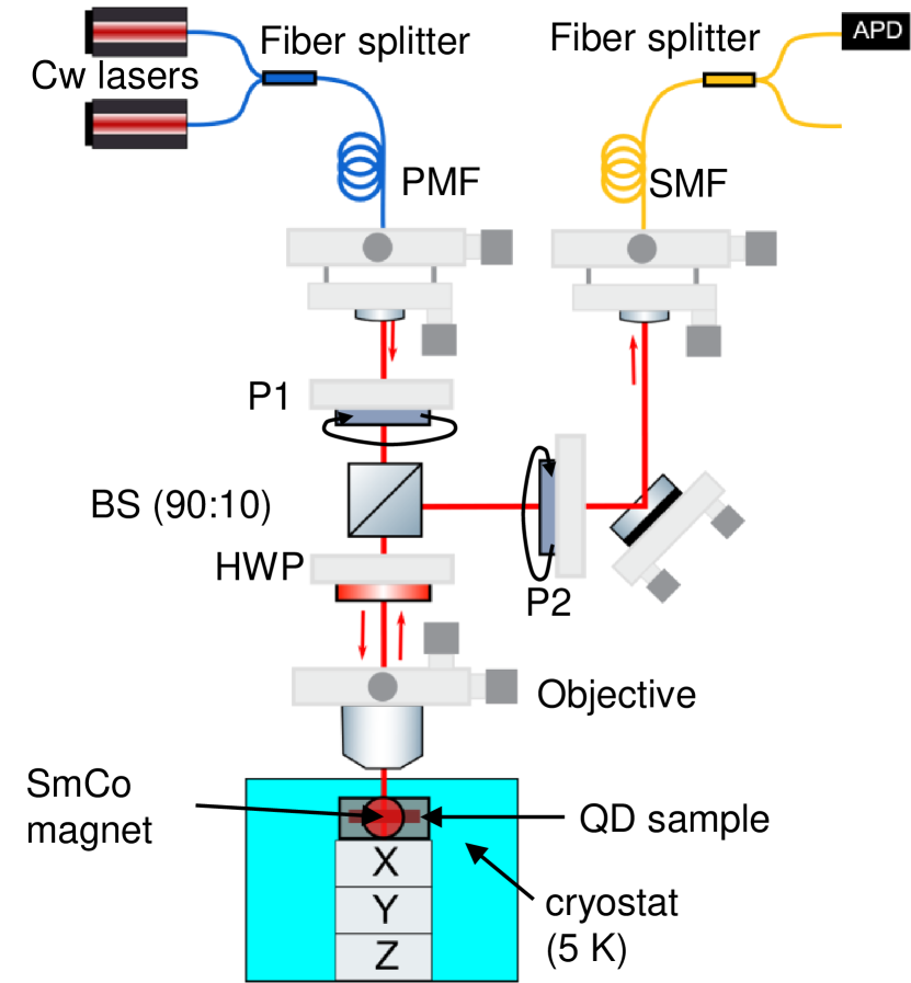
Figure B1: Experimental setup.

Appendix C Single-laser resonance fluorescence

The in-plane magnetic field of $475\,\mathrm{mT}$ splits the studied trion transition via the Zeeman effect into two pairs of linearly polarized emission lines with mutually orthogonal polarization. We observe a splitting of $3.4\pm 0.1\,\mathrm{GHz}$ and $1.8\pm 0.1\,\mathrm{GHz}$ between $V$-polarized and $H$-polarized transitions, respectively, corresponding to electron and hole g-factors of $|g_{\textrm{e}}|=0.39$ and $|g_{\textrm{h}}|=0.12$.

In the main text, we mainly focus on $V$-polarized resonant excitation with varied excitation power. We observe a constant Zeeman splitting over a bias range of more than $200\,\mathrm{mV}$, therefore we characterize the excitation power properties only for a bias voltage of $1.49\>\mathrm{V}$, a voltage where the transitions are in resonance with the $H$-polarized cavity mode. The pair of trion emission lines is detected in cross-polarization under $V$-polarized excitation of varied optical power $P_{l}$ over three orders in magnitude. We fit the measured resonance fluorescence spectrum with double Lorentzian function with a constant term characterizing an excitation laser leakage due to finite cross-polarization extinction ratio, and present the power dependency of the individual fit parameters in Fig. C1. We observe near-identical behavior for the emission lines in both photon rate and line broadening. Figure C1(a) shows the detected photon rate, which is well fit by $180\,\mathrm{kHz}/(1+P_{\textrm{c}}/P_{l})$ loudon_quantum_1973 , characterizing the two-level system saturation at power $P_{\textrm{c}}=22\pm 2\,\mathrm{nW}$. Similarly to our previous work Snijders2018 , we observe a power-linear background (gray), most likely due to imperfect polarization extinction. In Fig C1(b), we analyze excitation-power induced linewidth (FWHM) broadening. The experimental data show a linewidth of $\Gamma=1.55\pm 0.1\,\mathrm{GHz}$ at low excitation power, with a significant broadening above $P_{\textrm{c}}$. This broadening is well described with a simple power-law model $\Gamma+\beta P_{l}^{2/3}$ Sauncy1999 ; Huang2009 , using a parameter $\beta=(77\pm 10)\times 10^{3}\,\mathrm{GHz^{3/2}W^{-3/2}}$, and can be caused by an increase in the dephasing rate induced by nuclei polarization. The variation of the polarization of the nuclear-spin bath will also affect the eigenenergies, leading to significant changes in Zeeman splitting, as observed in Fig. C1(b).

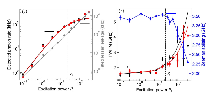
Figure C1: Single-laser power dependent characterization. Panel (a) shows how the detected rate of photons from the two trion transitions (black, red) and laser leakage (grey) depends on laser power. Panel (b) shows the power dependence of the full width at half maximum of these two Lorentzian transitions (black, red), and the Zeeman splitting (blue). Error bars show the statistical error of the fit parameters and solid lines show the model fits.

Appendix D Rate-equation model of resonant two-color spectroscopy of a negatively charged exciton

In this section, we describe our theoretical model used for comparison and understanding of the two-color resonance fluorescence experiments. Limiting the description to continuous-wave (cw) resonant excitation of the trion states in Voigt configuration, we model the trion energy levels as two coupled $\Lambda$ systems. Figure D1 shows a sketch of the interaction, where in total 4 optical transitions in a linear basis are possible: two emitting $V$-polarized (blue) and two emitting $H$-polarized photons (red), respectively. In addition to these optical transitions, there are also two spin-flip transitions, one for electron spin $\gamma_{\textrm{e}}$ and one for hole spin $\gamma_{\textrm{h}}$.

In the experiment, a strong laser power was used, therefore we can neglect quantization of the excitation light together with stimulated emission, but it was kept at least factor 3 below saturation intensity $P_{\textrm{c}}$. Within this limit, we can separate the problem into two steps: (i) setting up and solving rate equations characteristic to individual energy level configurations, and (ii) expression of emitted photon rates based on state populations found from (i).

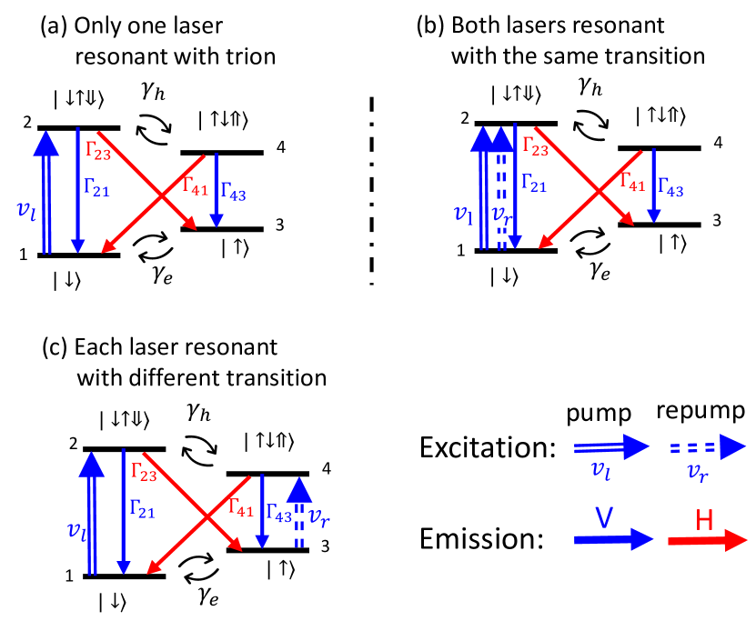
Figure D1: Resonant excitation schemes of trion: (a) a single excitation laser is resonant with a trion transition, (b) two lasers of identical polarization are resonant with the same transition, (c) two lasers are resonant with distinct trion transitions.

D.0.1 Spin population rate equations

The modeling of the scanning two-color resonant excitation of two coupled $\Lambda$ systems can be split into three scenarios, depicted in Fig. D1, distinguished by which transitions are addressed with the excitation lasers. Additionally, in correspondence to our experiment, the model is developed only for $V$-polarization, reducing the complexity.

We start with a situation when only a single laser is resonant with the trion energy levels, as depicted in Fig. D1(a). For simplicity, we discuss here only resonant excitation of the $|\downarrow\rangle\rightarrow|\downarrow\uparrow\Downarrow\rangle$ transition, $|\uparrow\rangle\rightarrow|\uparrow\downarrow\Uparrow\rangle$ can be derived easily. Here, the population is brought from the ground state $|\downarrow\rangle$ to the excited state with a single resonant laser of excitation rate $v_{l}$. The excited state relaxes back to the $|\downarrow\rangle$ or $|\uparrow\rangle$ spin state by spontaneous emission of a $V$ (emission rate $\Gamma_{21}$) and $H$ (emission rate $\Gamma_{23}$) polarized single photon, or via a hole spin-flip transition to $|\uparrow\downarrow\Uparrow\rangle$. We use the steady-state condition to solve the trion-state population described by the interaction matrix

$$M_{\mathrm{pump}}=\left(\begin{array}[]{cccc}-(v_{l}+\gamma_{\textrm{e}})&\Gamma_{21}&\gamma_{\textrm{e}}&\Gamma_{41}\\ v_{l}&-(\Gamma_{2}+\gamma_{\textrm{h}})&0&\gamma_{\textrm{h}}\\ \gamma_{\textrm{e}}&\Gamma_{23}&-\gamma_{\textrm{e}}&\Gamma_{43}\\ 0&\gamma_{\textrm{h}}&0&-(\Gamma_{4}+\gamma_{\textrm{h}})\end{array}\right)$$

and analytically find the state population $P_{|x\rangle}$ for each trion state involved in trion dynamics:

$$P_{|\downarrow\rangle} =\frac{\gamma_{\textrm{e}}\Gamma_{2}\Gamma_{4}+\gamma_{\textrm{e}}\gamma_{\textrm{h}}(\Gamma_{2}+\Gamma_{4})}{\alpha(v_{l})},$$

$$P_{|\downarrow\uparrow\Downarrow\rangle} =\frac{\gamma_{\textrm{e}}(\Gamma_{4}+\gamma_{\textrm{h}})}{\alpha(v_{l})}v_{l},$$

$$P_{\left|\uparrow\right\rangle} =P_{|\downarrow\rangle}+\frac{\Gamma_{23}}{\gamma_{\textrm{e}}}P_{|\downarrow\uparrow\Downarrow\rangle}+\frac{\Gamma_{43}\gamma_{\textrm{h}}}{\alpha(v_{l})}v_{l},$$

$$P_{|\uparrow\downarrow\Uparrow\rangle} =\frac{\gamma_{\textrm{e}}\gamma_{\textrm{h}}}{\alpha(v_{l})}v_{l}.$$ (D1)

Here, we use the total emission rates $\Gamma_{2}=\Gamma_{21}+\Gamma_{23}$ and $\Gamma_{4}=\Gamma_{41}+\Gamma_{43}$ from excited states $|\downarrow\uparrow\Downarrow\rangle$ and $|\uparrow\downarrow\Uparrow\rangle$, together with $\alpha(x)=[\Gamma_{43}\gamma_{\textrm{h}}+\Gamma_{23}(\Gamma_{4}+\gamma_{\textrm{h}})+\gamma_{\textrm{e}}\Gamma_{4}(2\Gamma_{2}+1)+2\gamma_{\textrm{e}}\gamma_{\textrm{h}}(\Gamma_{4}+\Gamma_{2}+1)]x$ to simplify the notation.

Now, we focus on two-laser excitation of the same transition, Fig. D1(b). Here, the two lasers have identical frequency and polarization and differ only in optical power, therefore we can model them as a single laser of optical power corresponding to $v_{l}+v_{r}$, where $v_{l}$ and $v_{r}$ are the excitation rates of pump and repump lasers. Then the state occupations have again form of eq. (D1), with the only change in the excitation rate $v_{l}\rightarrow v_{l}+v_{r}$.

For the two-color excitation scheme, where each laser is in resonance with a distinct trion transition, as sketched in Fig. D1(c). Because the interaction matrix

$$M_{\mathrm{pump\&repump}}=M_{\mathrm{pump}}+\left(\begin{array}[]{cccc}0&0&0&0\\ 0&0&0&0\\ 0&0&-v_{r}&0\\ 0&0&v_{r}&0\end{array}\right)$$

does not have a steady-state analytical solution, we obtain the state occupations $P_{|x\rangle}$ numerically.

D.0.2 2D two-color resonant excitation model

Now we formulate a simple model interconnecting our two-color resonance fluorescence experiment with the steady-state trion occupations derived from the system rate equations. First, we assume that the emitted resonance fluorescence rate is proportional to excited state occupations and the radiative transition rates as

$$I=(f_{V}\Gamma_{21}+f_{H}\Gamma_{23})P_{|\downarrow\uparrow\Downarrow\rangle}+(f_{V}\Gamma_{43}+f_{H}\Gamma_{41})P_{|\uparrow\downarrow\Uparrow\rangle.}$$

Here we use a parameter $f_{x}$ where the subscript indicates the emitted photon polarization allowing later implementation of the cross-polarization scheme by setting $f_{V}=0$ and $f_{H}=1$. We assume that the pair of the observed emission lines is resonantly excited with a laser of frequency $f_{1}^{\textrm{QD}}$ and $f_{2}^{\textrm{QD}}$, and each of the lines has a Lorentzian shape characterized by an identical full width at half maximum $\Gamma$, in agreement with our previous experiments in Sec. C. Using $\Gamma$, $f_{1}^{\textrm{QD}}$, and $f_{2}^{\textrm{QD}}$ from single-laser resonance fluorescence experiments, we model the emission as 2D Lorentzian functions $\mathrm{L}(x,x_{0},y,y_{0},\Gamma)=\frac{2}{\pi\Gamma}[(x-x_{0})^{2}+(y-y_{0})^{2}+(\Gamma/2)^{2}]^{-1}$ multiplied with photon rate $I$ calculated from the rate equations. As discussed above, the rate equations and thus also the state occupations and $I$ varies with specific resonant excitation configuration. The different conditions we label by $I^{(i,j)}$, where $i,j$ indicate with which transitions the laser are resonant with ($f_{x}^{\textrm{QD}}$) or 0 if the laser is not resonant with any trion transition. The final two-laser model is given by

$$I_{\mathrm{total}=} \sum_{i\in\{1,2\}}I^{(i,0)}\mathrm{L}(f_{r},f_{i}^{\textrm{QD}},0,0,\Gamma)$$

$$+\sum_{i\in\{1,2\}}I^{(0,i)}\mathrm{L}(0,0,f_{l},f_{i}^{\textrm{QD}},\Gamma)$$

$$-\sum_{i,j\in\{1,2\}}(I^{(i,0)}+I^{(0,j)})\mathrm{L}(f_{r},f_{i}^{\textrm{QD}},f_{l},f_{j}^{\textrm{QD}},\Gamma)$$ (D2)

$$+\sum_{i\in\{1,2\}}I^{(i,i)}\mathrm{L}(f_{r},f_{i}^{\textrm{QD}},f_{l},f_{i}^{\textrm{QD}},\Gamma)$$

$$+\sum_{i,j\in\{1,2\},i\neq j}I^{(i,j)}\mathrm{L}(f_{r},f_{i}^{\textrm{QD}},f_{l},f_{j}^{\textrm{QD}},\Gamma).$$

Here, the first two terms describe emission under single-laser excitation with separate lasers, the third term removes contributions of the individual lasers that would be counted twice otherwise. The fourth term accounts for emission by simultaneous two-resonant laser excitation of the identical transition, and the fifth term for concurrent two-color excitation of two distinct transitions.

D.0.3 Estimate of excitation and detection rates

To connect the theoretical model with our experiment, we need to estimate the trion driving power from optical power measured in the setup. It requires conversion of an optical power measured with a power meter to the individual laser excitation rates $v_{l}$ and $v_{r}$. First, we determine the setup throughput as described in Sec. B. As an example, the optical power is $P=21\,\mathrm{nW}$, measured in our setup in front of BS. Using the measured transmission of the excitation path of our setup ($\eta_{\textrm{ex}}=T_{\textrm{cav}}\eta_{\textrm{obj}}\eta_{\textrm{BS,T}}$), and assuming unity QD quantum efficiency, we estimate that the QD is excited with an optical power corresponding to $\eta_{\textrm{ex}}P=0.44\,\mathrm{pW}$. The excitation rate is then calculated from this power by multiplication with an experimentally determined conversion factor between power-meter readings and the single-photon rate measured with a single-photon detector.

Similarly, we correct the theoretical emission for the detection system optical throughput simply by its multiplication with experimentally determined throughput $\eta_{\textrm{det}}$.

D.0.4 Model rates estimation

We start the discussion with the radiative rates of our trion-cavity system. An isolated trion in Voigt geometry typically has all four radiative transitions of an identical rate around $\Gamma_{0}=1\,\mathrm{GHz}$ Bayer2002 . The situation is different if a trion is coupled into a linearly polarized cavity mode leading to Purcell enhancement. Neglecting pure dephasing, we estimate the cavity-enhanced rates from the QD emission line width $\Gamma$ of $1.5\>\mathrm{GHz}$, giving $\Gamma_{21}=\Gamma_{43}=3\,\mathrm{GHz}$. Assuming that the second pair of rates correspond to an isolated trion, we estimate these rates to be $\Gamma_{23}=\Gamma_{41}=1\,\mathrm{GHz}$. Since these rates are very sensitive to the specific condition, we keep them as free fit parameters for the two-color experiments show in the main text and below.

Now we discuss how we estimate the electron and hole-spin flip rates based on comparison of the power dependence of the single laser resonance fluorescence with our model for single laser excitation, i.e., using only the first term in eq. (D2). We model the trion level system with the radiative rates estimated above and vary only $\gamma_{\textrm{e}}$ and $\gamma_{\textrm{h}}$.

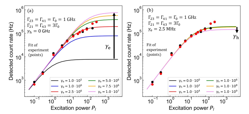
Figure D2: Spin-flip rate estimate from excitation power dependent trion emission under single resonant excitation. Lorentzian fits of experimental data (data points) are compared to our model with (a) varied $\gamma_{\textrm{e}}$ and fixed $\gamma_{\textrm{h}}=0$ to estimate $\gamma_{\textrm{e}}$ value, and in (b) with varied $\gamma_{\textrm{h}}$ and fixed $\gamma_{\textrm{e}}=2.5\,\mathrm{MHz}$.

First, we estimate the electron spin-flip rate. Typically $\gamma_{\textrm{h}}\ll\gamma_{\textrm{e}}\ll\Gamma_{0}$ , therefore we can neglect the hole spin-flip transition and set in our model $\gamma_{\textrm{h}}=0$. Then, we determine the most likely value of $\gamma_{\textrm{e}}$ by comparing a simulated power dependence of the detected rate for various $\gamma_{\textrm{e}}$ with the experimentally observed rates, as shown in Fig. D2(a). In good agreement with $\gamma_{e}=1.2\,\mathrm{MHz}$ reported in Kroner2008PRB , we achieved the best agreement between the model and experimental data for $\gamma_{\textrm{e}}=2.5\,\mathrm{MHz}$. In Fig. D2(b), we present a similar simulation, now with fixed $\gamma_{\textrm{e}}=2.5\,\mathrm{MHz}$ and varied $\gamma_{\textrm{h}}$ to reveal the model dependency on $\gamma_{\textrm{h}}$. In contrast to Fig. D2(a), we observe only weak dependence of the model on $\gamma_{\textrm{h}}$, so we set in all our simulations for simplicity $\gamma_{\textrm{h}}=0$. This agrees with the fact that we can only observe hole-spin flips during the very short trion lifetime.

D.0.5 Excitation-power dependent two-color resonant excitation

Here we study the excitation power dependency of trion state occupations under different resonant excitation schemes and compare the model with the measured two-laser excitation resonance fluorescence. The parameters to model the trion steady-state population are estimated from a least-square fit (discussed below) of the experimental data with an optical power of $P_{r}=2.0$ and $P_{l}=2.1\,\mathrm{nW}$, and the best agreement is achieved for parameters $\Gamma_{21}=2.1\,\textrm{GHz},\Gamma_{43}=2.7\mathrm{\,GHz}$, $\Gamma_{23}=\Gamma_{41}=0.8\,\mathrm{GHz}$, $\gamma_{\textrm{e}}=2.5\,\mathrm{MHz},$ and $\gamma_{\textrm{h}}=0\,\mathrm{Hz}$.

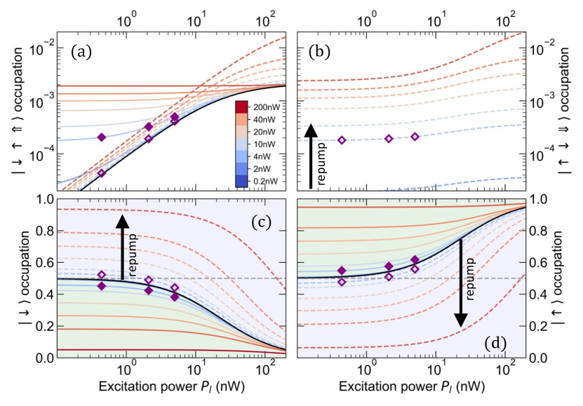
Figure D3: Simulation of the two-laser power dependency of trion state occupations. Three different excitation schemes are compared: single laser excitation (1LRE, black solid line), two-laser excitation of an identical line (2LRE, colored solid lines), and two-color excitation of two distinct transitions (2CRE, colored dashed lines). The power of the second laser is encoded in the color scale. Two regions of ground state occupation are highlighted (c,d): the orange region is accessible only with two-laser excitation of an identical transition, and the blue one only if two distinct transitions are resonantly excited. Purple diamonds (filled if two lasers address the same transition, empty if different ones) correspond to experimental conditions.

Assuming only minor power-induced rate changes for excitation below $P_{\textrm{c}}$, in Fig. D3 we study the state population of the individual trion levels as a function of the optical power of both lasers. Under weak single-laser excitation where the excitation rate is much slower than the radiative rate of the transition, the radiative relaxation of the excited state into both ground states is much faster than the excitation. Therefore the dynamics is dominated by spontaneous emission. Since the radiative rates of the transitions are approximately equal, we observe in (c) and (d) an expected balanced ground state population of $\sim 0.5$ Kroner2008PRB . With increasing excitation power, repumping of the $|\downarrow\rangle$ population into the excited state becomes relevant, leading to a ground state population imbalance together with a rise of the excited state population, which saturates at high powers, see Fig. D3(a). As discussed also in the main text, the dynamics under two-laser excitation of a single transition is equivalent to single-laser excitation with higher excitation power. However, the dynamics changes under the two-color excitation of two distinct transitions shown as dashed lines in Fig. D3, where the second laser repumps the population from $\left|\uparrow\right\rangle$ to $|\uparrow\downarrow\Uparrow\rangle$. As our model predicts, this repumping is higher with a stronger repumping laser.

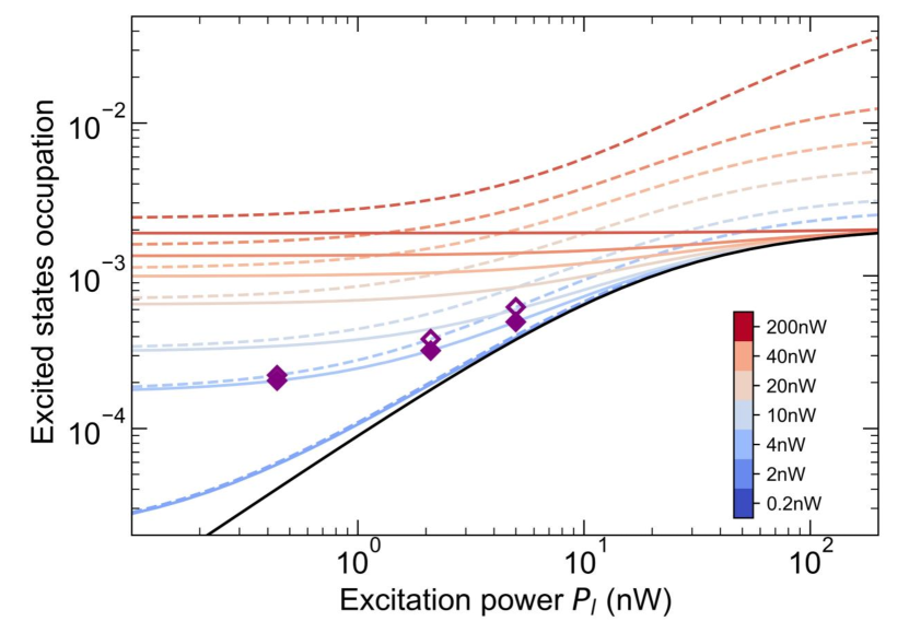
Figure D4: Simulated power dependency of the total excited states population. Color and line style encoding is identical to that in Fig. D3.

Since emission is a measure of the population of the excited states, we can gain insight about expected detected photon rates in different resonant excitation schemes from the total occupation of excited states, shown in Fig. D4. Interestingly, the total excited state population is always higher in the two-color excitation scheme. That is because the second laser populates the second excited state which was (due to negligible $\gamma_{\textrm{h}}$) not involved in dynamics if only a single transition was resonantly pumped. This shows that a repump laser can enhance the single-photon rate.

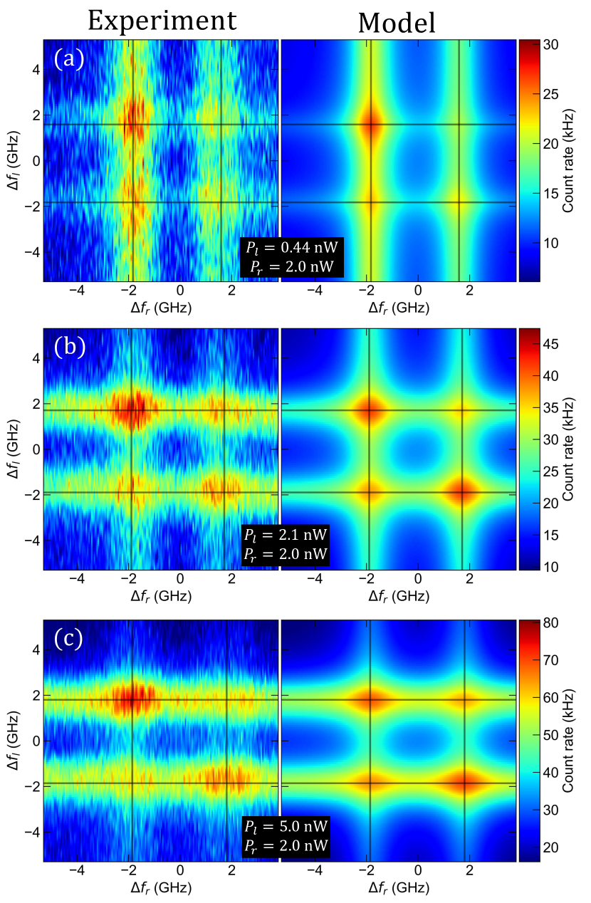
Figure D5: False-color plots of the resonant two-color laser scans and model results. Experimental data is shown in the left column, the model in the right column. The repump laser power is kept constant at $P_{r}=2.0\,\mathrm{nW}$, while the pumplaser power $P_{l}$ is varied: (a) $P_{l}=0.44\,\mathrm{nW}$, (b) $P_{l}=2.1\,\mathrm{nW}$, and (c) $P_{l}=5.0\,\mathrm{nW}$. The transition frequencies of the QD are shown by solid black lines.

Finally, we discuss additional two-color experiments. In Fig. D5, we observe again a ’number sign’ like structure, where horizontal and vertical lines represent the trion transitions probed with probe and pump laser, and at the intersections two-laser dynamics appears. Again, spin repumping is clearly visible. We fit the model with an extra term describing the background caused by imperfect cross-polarization filtering on three sets of experimental data measured with fixed pump laser power of $P_{r}=2.0\,\mathrm{nW}$ and we have varied optical power of probe laser $P_{l}$. We use the following steps to achieve the best agreement between the model and our experiment: First, we fit the experiment using the initial estimate of radiative and spin-flip rates, and QD linewidth and energies, as discussed above. We optimize Zeeman splitting together with the linewidths, therefore we keep all parameters (except $\gamma_{\textrm{h}}=0\,\mathrm{Hz}$) free. In the next step, we fix the parameter describing the background, and QD’s $f_{1}^{\textrm{QD}}$, $f_{2}^{\textrm{QD}}$, $\Gamma$, and optimize only radiative rates and $\gamma_{\textrm{e}}$. The best fits of the model are compared to the experiment in Fig. D5. Examination of the power-dependence of the parameters shows a power broadening (FWHM) from $1.52\,\mathrm{GHz}$ to $1.89\,\mathrm{GHz}$ and a small increase of the Zeeman splitting from $3.40\,\mathrm{GHz}$ to $3.65\,\mathrm{GHz}$, as also shown in Fig. C1. The determined electron and hole spin-flip rates are $\gamma_{\textrm{e}}=2.5\>\mathrm{\textrm{MHz}}$ and $\gamma_{\textrm{h}}=0\,\mathrm{Hz}$; radiative rates are increasing with excitation power and are $\Gamma_{21}=1.1-4.9\,\textrm{GHz},\Gamma_{43}=2.1-4.5\mathrm{\,GHz}$, $\Gamma_{23}=\Gamma_{41}=0.7-0.8\,\mathrm{GHz}$, probably due to the Rabi effect.