On-shell approximation for the s-wave scattering theory

Abstract

We investigate the scattering theory of two particles in a generic $D$-dimensional space. For the s-wave problem, by adopting an on-shell approximation for the $T$-matrix equation, we derive analytical formulas which connect the Fourier transform ${\tilde{V}}(k)$ of the interaction potential to the s-wave phase shift. In this way we obtain explicit expressions of the low-momentum parameters ${\tilde{g}}_{0}$ and ${\tilde{g}}_{2}$ of ${\tilde{V}}(k)={\tilde{g}}_{0}+{\tilde{g}}_{2}k^{2}+...$ in terms of the s-wave scattering length $a_{s}$ and the s-wave effective range $r_{s}$ for $D=3$, $D=2$, and $D=1$. Our results, which are strongly dependent on the spatial dimension $D$, are a useful benchmark for few-body and many-body calculations. As a specific application, we derive the zero-temperature pressure of a 2D uniform interacting Bose gas with a beyond-mean-field correction which includes both scattering length and effective range.

I Introduction

One of the main features of the physics of ultracold and dilute atomic gases is their universality, i.e. the fact that the interaction potential, and consequently many physical properties, can be accurately described by only one zero-range interaction parameter: the s-wave scattering length [1, 2]. The flexibility of current experimental techniques prompts novel interest in the nonuniversal behavior of quantum gases. One remarkable example is the possibility of using Feshbach resonances for tuning the s-wave scattering length, and eventually obtain an interaction regime in which the next-to-leading order term in the low momentum expansion of the potential, i.e. the effective range $r_{s}$, becomes relevant [3]. The effects of the inclusion of the effective range are various: the equation of state of a Bose gas undergoes substantial modifications [4, 5, 6, 7, 8], and so does the description of the dynamics. In particular, by considering the effective range contribution in the mean-field dynamics, one obtains the so-called modified Gross-Pitaevskii equation [9, 10], that have been used to predict dynamical signatures of effective range in the case of solitons and sound waves [11]. Some diffusion Monte Carlo calculations were carried out for studying the validity of a universal description of the bosonic gas, i.e. using the gas parameter $na_{s}^{3}$, where $n$ is the 3D density and $a_{s}$ the s-wave scattering length. Although in Ref. [12] the universal approach is shown to be valid for usual experimental settings, more recent Monte Carlo investigations with a Bose-Bose mixture [13] suggest that by increasing the number density the effective range $r_{s}$ is needed to accurately reproduce the numerical results (see also the analytical results of Ref. [14]).

Taking into account that the interaction potential is not directly measurable in usual experiments, in recent years separable potentials [15] were assumed to investigate nonuniversal features of bosonic and fermionic systems [16, 17, 18]. In these papers, which adopt the effective field theory (EFT) methodology, dimensional regularization (DR) and minimal subtraction (MS) were employed to regularize the divergent loop integrals. In the low-energy limit, which corresponds to consider only s-wave contribution to the phase shift, these calculations are based on the writing of an effective action of which only the terms contributing to the desired low-momentum expansion are retained. This EFT procedure was previously used to study the nucleon-nucleon scattering problem [19, 20, 21, 22, 23]. It is important to stress that, in the three dimensional case, the nonuniversal EFT corrections of Refs. [16, 17] do not agree with the ones of Refs. [10, 24, 25, 26], which are based on the simple Born (zero-order) approximation of scattering theory. This disagreement is due to different methods and assumptions in the two approaches. In the first setting [16, 17], the aim is to obtain the correct low-momentum expansion of the phase shift, by starting from an effective Lagrangian, and summing the Feynman graphs for the $T$-matrix up to the desired momentum power. The second approach [10, 24, 25, 26] is instead based on the calculation of the energy shift due to a phase shift in the wavefunction in a finite volume, and then letting the volume go to infinity. A puzzling consequence of this energy-shift approach in three spatial dimensions is the fact that sending the s-wave effective range $r_{s}$ to zero the finite-range correction of the low-momentum expansion of the interaction potential remains finite. In this paper we adopt the EFT approach [16, 17] because it is strictly related to the scattering theory via the $T$-matrix, it can be directly applied also to reduced spatial dimensions, and the obtained finite-range corrections are always vanishing for $r_{s}\to 0$.

Exact analytical calculations able to tackle the scattering theory by using a realistic finite-range interaction potential are not available [27, 28, 29]. In this paper we face this problem under the assumption of low energy scattering and using an arbitrary dimension partial wave expansion. Our method, which is based on two crucial approximations on the $T$-matrix equation, called s-wave and on-shell approximations, allows one to link in a systematic way the s-wave components of the interaction potential and the transition matrix in any spatial dimension $D$. In particular, for $D=3$, $D=2$, and $D=1$ we obtain explicit expressions of the low-momentum parameters of the Fourier transform ${\tilde{V}}(k)$ of the interaction potential $V(r)$ in terms of the s-wave scattering length $a_{s}$ and effective range $r_{s}$. In this way we recover the nonuniversal EFT results in three spatial dimensions [16, 17]. In the last section, we apply our theory to derive the zero-temperature pressure of the interacting gas in two dimensions in terms of $a_{s}$ and $r_{s}$ (see also Ref. [8]).

II The two-body problem

Let us consider the Hamiltonian operator

$${\hat{H}}={\hat{H}}_{0}+{\hat{V}}\;,$$ (1)

where ${\hat{H}}_{0}={\hat{\bf p}}^{2}/(2m_{r})$ is the kinetic energy operator of a particle of reduced mass $m_{r}$ and linear momentum ${\hat{\bf p}}$ while ${\hat{V}}$ the interaction potential operator. We assume that the potential operator ${\hat{V}}$ is diagonal in the coordinate representation, namely ${\hat{V}}|{\bf r}\rangle=V({\bf r})|{\bf r}\rangle$, where $|{\bf r}\rangle$ is the eigenstate of the position operator ${\hat{\bf r}}$, i.e. ${\hat{\bf r}}|{\bf r}\rangle={\bf r}|{\bf r}\rangle$. Moreover, $m_{r}=m/2$ is the reduced mass of two identical particles, each of mass $m$.

As shown in many text books [30, 3, 31], in $D$ spatial dimensions, the matrix element $T_{{\bf k}{\bf k}^{\prime}}=\langle{\bf k}|{\hat{T}}|{\bf k}^{\prime}\rangle$ of the transition operator ${\hat{T}}$ of scattering theory satisfies the $T$-matrix equation

$$T_{{\bf k}{\bf k}^{\prime}}=V_{{\bf k}{\bf k}^{\prime}}+\int d^{D}{\bf k}^{\prime\prime}{V_{{\bf k}{\bf k}^{\prime\prime}}\over{\hbar^{2}k^{2}\over 2m_{r}}-{\hbar^{2}(k^{\prime\prime})^{2}\over 2m_{r}}+{\color[rgb]{0,0,0}i\,\epsilon}}T_{{\bf k}^{\prime\prime}{\bf k}^{\prime}}\;,$$ (2)

where $V_{{\bf k}{\bf k}^{\prime}}=\langle{\bf k}|{\hat{V}}|{\bf k}^{\prime}\rangle$, $|{\bf k}\rangle$ is the initial state, $|{\bf k}^{\prime}\rangle$ is the final state, and $|{\bf k}^{\prime\prime}\rangle$ is an intermediate state. The involved variables are represented pictorially in Fig. 1.

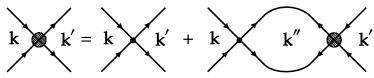
Figure 1: Depiction of the scattering process in the center-of-mass reference frame used in the construction of Eq. (2). The initial state, represented in the left of all diagrams, is a relative motion in the state $\ket{\mathbf{k}}$, and the final state, in the right side of the diagrams, is in the state $\ket{\mathbf{k^{\prime}}}$. The shadowed center represents the $T$-matrix, whereas the black dot represents the potential. The last term specifies the relation between initial, final, and intermediate state $\ket{\mathbf{k^{\prime\prime}}}$.

Here, $|{\bf k}\rangle$, $|{\bf k}^{\prime}\rangle$, and $|{\bf k}^{\prime\prime}\rangle$ are eigenstates of the linear momentum operator ${\hat{\bf p}}$, i.e. ${\hat{\bf p}}|{\bf k}\rangle=\hbar{\bf k}|{\bf k}\rangle$, ${\hat{\bf p}}|{\bf k}^{\prime}\rangle=\hbar{\bf k}^{\prime}|{\bf k}^{\prime}\rangle$, and ${\hat{\bf p}}|{\bf k}^{\prime\prime}\rangle=\hbar{\bf k}^{\prime\prime}|{\bf k}^{\prime\prime}\rangle$. In Eq. (2), $i$ is the imaginary unit and $\epsilon>0$ is an infinitesimal real parameter ensuring that in the scattering there are only outgoing waves. Notice that $V_{{\bf k}{\bf k}^{\prime}}={\tilde{V}}({\bf k}-{\bf k}^{\prime})/(2\pi)^{D}$, where

$${\tilde{V}}({\bf k})=\int d^{D}{\bf r}\ V(r)\ e^{-i{\bf k}\cdot{\bf r}}\;.$$ (3)

is the Fourier transform of the interaction potential $V({\bf r})$. We assume that the interaction potential $V({\bf r})$ is spherically symmetric, i.e. $V({\bf r})=V(r)$ with $r=|{\bf r}|$, and it follows that ${\tilde{V}}({\bf k})={\tilde{V}}(k)$.

II.1 Partial waves decomposition

The $T$-matrix equation (2) can be decomposed in partial waves in $D$ dimensions in the following way (see Appendix A for further details). We drop $D$ when the notation is not ambiguous. Define the partial wave expansion of $V_{\mathbf{k}\mathbf{k}^{\prime}}$ as

$$V_{\mathbf{k}\mathbf{k}^{\prime}}=\dfrac{1}{(2\pi)^{D}}\sum_{l}V_{l}(k,k^{\prime})\,N(D,l)P_{l}(\mathbf{\hat{k}}\cdot\mathbf{\hat{k}}^{\prime}),$$ (4)

holding also for $T_{\mathbf{k}\mathbf{k}^{\prime}}$ in an analogous way. The number of spherical harmonics in $D$ dimensions with $D>1$, is the number of independent homogeneous and harmonic polynomials of degree $l$ in $D$ variables, that is [45]:

$$N(D,l)=\dfrac{2l+D}{l}\binom{D+l-3}{l-1}.$$ (5)

For $D=3$ we recover the usual multiplicities of the spherical harmonics. It is easy to verify that when $l=0$, one has $N(3,0)=1$, $N(2,0)=2$.

Substituting into Eq. (2), using the orthogonality of Legendre functions and the uniqueness of the representation in partial waves, one obtains

$$T_{l}(k,k^{\prime})P_{l}(\mathbf{\hat{k}}\cdot\mathbf{\hat{k}}^{\prime})=V_{l}(k,k^{\prime})P_{l}(\mathbf{\hat{k}}\cdot\mathbf{\hat{k}}^{\prime})$$ (6)

$$+\int{d^{D}\mathbf{k}^{\prime\prime}\over(2\pi)^{D}}\Biggl{[}\dfrac{N(D,l)}{{\hbar^{2}k^{2}\over m}-{\hbar^{2}(k^{\prime\prime})^{2}\over m}+{\color[rgb]{0,0,0}i\,\epsilon}}V_{l}(k,k^{\prime\prime})T_{l}(k^{\prime\prime},k^{\prime})$$

$$\times P_{l}(\mathbf{\hat{k}}\cdot\mathbf{\hat{k}}^{\prime\prime})P_{l}(\mathbf{\hat{k}}^{\prime\prime}\cdot\mathbf{\hat{k}}^{\prime})\Biggr{]}\;.$$

Choosing $k=k^{\prime}$, the angular integral can be computed using the orthonormalization of Legendre polynomials (see Eq. (47) of Appendix B). By selecting the s-wave term $l=0$ we get

$$T_{0}(k)=V_{0}(k)$$ (7)

$$+S_{D}\int_{0}^{\infty}{dk^{\prime\prime}\over(2\pi)^{D}}\dfrac{(k^{\prime\prime})^{D-1}}{{\hbar^{2}k^{2}\over m}-{\hbar^{2}(k^{\prime\prime})^{2}\over m}+{\color[rgb]{0,0,0}i\,\epsilon}}V_{0}(k,k^{\prime\prime})T_{0}(k^{\prime\prime},k)\;,$$

where $T_{0}(k)=T_{0}(k,k)$, $V_{0}(k)=V_{0}(k,k)$, and $S_{D}=2\pi^{D/2}/\Gamma(D/2)$ is the solid angle in $D$ dimensions with $\Gamma(x)$ the Euler gamma function.

III On-shell approximation

Here we adopt the s-wave approximation but also the “on-shell approximation” [31]. Explicitly we assume that, due to the singularity in the integrand for $k=k^{\prime\prime}$, in Eq. (7) $V_{0}(k,k^{\prime\prime})\simeq V_{0}(k,k)=V_{0}(k)$ and $T_{0}(k^{\prime\prime},k)\simeq T_{0}(k,k)=T_{0}(k)$. As a consequence, Eq. (7) becomes

$$T_{0}(k)=V_{0}(k)+V_{0}(k)\ C(k)\ T_{0}(k)$$ (8)

with

$$C(k)=S_{D}\int_{0}^{\infty}{d{k^{\prime\prime}}\over(2\pi)^{D}}{1\over{\hbar^{2}k^{2}\over m}-{\hbar^{2}(k^{\prime\prime})^{2}\over m}+{\color[rgb]{0,0,0}i\,\epsilon}}\;.$$ (9)

Then one finds

$$T_{0}(k)={1\over{1\over V_{0}(k)}-C(k)}\;,$$ (10)

which is the crucial formula of our paper. Eq. (10) can be obtained from Eq. (8) in two ways: by a direct algebraic manipulation or by summing up the associated Born-like geometric series within an iterative scheme. We stress that Eq. (10), based on the s-wave and the on-shell approximation, is expected to be reliable in the regime of low momentum and it becomes exact for $k\to 0$ [3]. Indeed, it turns out that Eq. (10) is structurally similar to Eq. (3.16) of Ref. [20], obtained within the EFT procedure.

It is important to observe that the s-wave component $V_{0}(k)$ does not coincide with the Fourier transform ${\tilde{V}}(k)$. Actually for $D=3$ and $D=2$ we find (see Appendix B)

$$V_{0}(k)=\frac{1}{2}\int_{0}^{\pi}d\theta\ {\tilde{V}}(2k\sin(\theta/2))\ \sin{(\theta)}\;.$$ (11)

Taylor expanding with respect to $k$ the s-wave component $V_{0}(k)$ we formally obtain

$$V_{0}(k)=g_{0}+g_{2}\ k^{2}+...\;,$$ (12)

where the coefficients $g_{0}$ and $g_{2}$ depend on the choice of the Fourier transform ${\tilde{V}}(k)$ of the interaction potential. Performing also the Taylor expansion of the latter, i.e.

$${\tilde{V}}(k)={\tilde{g}}_{0}+{\tilde{g}}_{2}\ k^{2}+...\;,$$ (13)

one finds, using Eq. (11) that $g_{0}={\tilde{g}}_{0}$ and $g_{2}=2{\tilde{g}}_{2}$. As shown in Appendix B, these two simple relationships are valid also for $D=1$.

III.1 Dimensional regularization

In the limit $\epsilon\to 0$, the term $C(k)$ of Eq. (9) can be written as

$$C(k) = -{S_{D}\over(2\pi)^{D}}{m\over\hbar^{2}}\int_{0}^{\infty}dk^{\prime\prime}(k^{\prime\prime})^{D-1}{1\over(k^{\prime\prime})^{2}+(-ik)^{2}}$$ (14)

$$= -{m\over\hbar^{2}}(-ik)^{D-2}{B(D/2,1-D/2)\over(4\pi)^{D/2}\Gamma(D/2)}\;,$$

where $B(x,y)$ is the Euler beta function. Clearly, $C(k)$ is ultraviolet divergent at any integer dimension $D$. We now show how this divergence is eliminated by DR [32, 33].

The Euler beta function

$$B(x,y)=\int_{0}^{+\infty}dt{t^{x-1}\over(1+t)^{x+y}}$$ (15)

is defined with the real parts of $x$ and $y$ greater than zero. However, it can be analytically continued [33] to complex values of $x$ and $y$ as

$$B(x,y)={\Gamma(x)\Gamma(y)\over\Gamma(x+y)}\;.$$ (16)

Performing this analytic continuation in Eq. (14) means that we promote the integer spatial dimension $D$ to a complex number [32, 33]. After doing it, we can safely go back to an integer $D$, if $D=3$ and $D=1$ [33]. Thus, we get [32]

$$C(k)=-{m\over\hbar^{2}}(-ik)^{D-2}{\Gamma(1-D/2)\over(4\pi)^{D/2}}\;,$$ (17)

where $D$ is in general, for the specific discussion of this subsection, a complex number very close to its integer counterpart.

From Eq. (17), simply setting $D=3$ and remembering that $\Gamma(-1/2)=-2\sqrt{\pi}$, we obtain

$$C(k)=-ik{m\over 4\pi\hbar^{2}}\;.$$ (18)

Setting $D=1$, and remembering that $\Gamma(1/2)=\sqrt{\pi}$, we have instead

$$C(k)=-i{1\over k}{m\over 2\hbar^{2}}\;.$$ (19)

DR is more difficult in two spatial dimensions. In fact, for $D=2$ Eq. (17) diverges due to the presence of $\Gamma(0)$. To face this divergence, we extend the calculation to non-integer dimension $D=2-\epsilon$ and let $\epsilon$ go to zero only at the end of the calculation. Eq. (17) can be written as

$$C(k)=-{m\over\hbar^{2}}\kappa_{0}^{\epsilon}(-ik)^{-\epsilon}{\Gamma(\epsilon/2)\over(4\pi)^{1-\epsilon/2}}\;,$$ (20)

where the regulator $\kappa_{0}$ is a scale wavenumber which enters for dimensional reasons. The small-$\epsilon$ expansion of the gamma function reads

$$\Gamma(\epsilon/2)={2\over\epsilon}-\gamma+O(\epsilon)\;,$$ (21)

where $\gamma\simeq 0.5572$ is the Euler-Mascheroni constant. Taking into account that $x^{\epsilon}=e^{\ln(x^{\epsilon})}=e^{\epsilon\ln(x)}=1+\ln(x)\epsilon+O(\epsilon^{2})$ and $\ln(-i)=-i\pi/2$, we finally get

$$C(k)={m\over 2\pi\hbar^{2}}\ln({k\over 2}{e^{\gamma/2}\over\Lambda})-{m\over 4\hbar^{2}}i\;,$$ (22)

after removing the remaining singularity (MS scheme) [34] and setting $\Lambda=\sqrt{\pi}\kappa_{0}$, which plays the role of a ultraviolet cutoff.

IV Interaction potential and phase shift for $D=3$

By using the $D=3$ results of the previous section we can write

$$T_{0}(k)={1\over{1\over V_{0}(k)}+ik{m\over 4\pi\hbar^{2}}}\;.$$ (23)

It is important to underline, that Eq. (23) is a generalization of the result obtained in Ref. [17] with the simple potential $V_{0}(k)=g_{0}+g_{2}k^{2}$.

A well known result of the scattering theory is that the s-wave transition element $T_{0}(k)$ can be written in term of the s-wave scattering amplitude $f_{0}(k)$ as follows [3]

$$T_{0}(k)=-{4\pi\hbar^{2}\over m}f_{0}(k)\;.$$ (24)

Moreover, the s-wave scattering amplitude $f_{0}(k)$ is related to the s-wave phase shift $\delta_{0}(k)$ by the formula [3]

$$f_{0}(k)={1\over k\cot(\delta_{0}(k))-ik}\;.$$ (25)

Using these two equations with Eq. (23), valid in $D=3$, we get

$$V_{0}(k)=-{4\pi\hbar^{2}\over m}{\tan(\delta_{0}(k))\over k}\;.$$ (26)

This is our main 3D result: an explicit relationship between $V_{0}(k)$ of the 3D spherically-symmetric interaction potential and the 3D s-wave phase shift $\delta_{0}(k)$. Quite remarkably, Eq. (26) is quite similar to the ansatz ${\tilde{V}}(k)=-(4\pi\hbar^{2}/m)\delta_{0}(k)/k$ suggested in Ref. [24].

By definition, the 3D s-wave scattering length $a_{s}$ and the 3D s-wave effective range $r_{s}$ are the low-momenta coefficients of the following expansion of the 3D phase shift $\delta_{0}(k)$ [30, 3, 31]:

$$k\ \cot({\delta_{0}(k)})=-{1\over a_{s}}+{1\over 2}r_{s}k^{2}+...\;.$$ (27)

This effective range expansion is valid for interaction potentials that decay more rapidly than $r^{-5}$ [24]. Taking into account this low momentum expansion, from Eq. (26) and the Taylor expansion of $V_{0}(k)$ with respect to k, Eq. (12), we get

$$g_{0}={4\pi\hbar^{2}\over m}a_{s}$$ (28)

and

$$g_{2}={2\pi\hbar^{2}\over m}a_{s}^{2}r_{s}\;.$$ (29)

Eq. (28), which relates $g_{0}$ to $a_{s}$, is quite familiar [30, 3, 31]. Instead Eq. (29), which relates $g_{2}$ to $a_{s}$ and $r_{s}$ is less known, but it can be found in Refs. [17, 4]. Notice that these results, and in particular Eq. (26), hold in the regime where $a_{s}$ is finite while $k$ is small. In other words, Eq. (26) cannot be used to model the unitarity regime, where the scattering length $a_{s}$ diverges, while Eq. (27) for $a_{s}=\infty$ and $r_{s}=0$ simply gives $\delta_{0}(k)=\pi/2$.

V Interaction potential and phase shift for $D=1$

By using the $D=1$ results of Section III we have

$$T_{0}(k)={1\over{1\over V_{0}(k)}+i{1\over k}{m\over 2\hbar^{2}}}\;.$$ (30)

An interesting achievement of the 1D scattering theory is that the s-wave transition element $T_{0}(k)$ is related to the s-wave phase shift $\delta_{0}(k)$ by the formula [35, 36]

$$T_{0}(k)=-\left({2\hbar^{2}\over m}\right)\left({k\over\cot(\delta_{0}(k))-i}\right)\;.$$ (31)

Comparing this equation with Eq. (30) we get

$$V_{0}(k)=-{2\pi\hbar^{2}\over m}k\ \tan(\delta_{0}(k))\;.$$ (32)

This is our main 1D result: an explicit relationship between the Fourier transform $V_{0}(k)$ of the 1D spherically-symmetric interaction potential and the 1D s-wave phase shift $\delta_{0}(k)$.

By definition, the 1D s-wave scattering length $a_{s}$ and the 1D s-wave effective range $r_{s}$ are the low-momenta coefficients of the following expansion of the 1D phase shift $\delta_{0}(k)$ [35, 36]

$$k\ \tan({\delta_{0}(k)})={1\over a_{s}}+{1\over 2}r_{s}k^{2}+...\;.$$ (33)

Taking into account this low momentum expansion, from Eq. (32) and the Taylor expansion of $V_{0}(k)$, Eq. (12), we obtain

$$g_{0}=-{2\hbar^{2}\over ma_{s}}$$ (34)

and

$$g_{2}=-{\hbar^{2}\over m}r_{s}\;.$$ (35)

Eq. (34), which relates $g_{0}$ to $a_{s}$, is quite familiar [35, 36]. Instead Eq. (35), which relates $g_{2}$ to $r_{s}$, was previously found in Ref. [5].

VI Interaction potential and phase shift for $D=2$

By using the $D=2$ results of Section III the s-wave transition element reads

$$T_{0}(k)={1\over{1\over V_{0}(k)}-{m\over 2\pi\hbar^{2}}\ln({e^{\gamma/2}k\over 2\Lambda})+{m\over 4\hbar^{2}}i}\;.$$ (36)

In the 2D scattering theory the s-wave transition element $T_{0}(k)$ is related to the s-wave phase shift $\delta_{0}(k)$ by the formula [37]

$$T_{0}(k)=-\left({4\hbar^{2}\over m}\right)\left({1\over\cot(\delta_{0}(k))-i}\right)\;.$$ (37)

Comparing this equation with Eq. (36) we find

$$V_{0}(k)=-\left({4\hbar^{2}\over m}\right){1\over\cot(\delta_{0}(k))-{2\over\pi}\ln({k\over 2}{e^{\gamma/2}\over\Lambda})}\;.$$ (38)

This is our main 2D result: $V_{0}(k)$ of the 2D spherically-symmetric interaction potential in terms of the 2D s-wave phase shift $\delta_{0}(k)$. Eq. (38) clearly depends on the ultraviolet cutoff $\Lambda$.

By definition, for short-range potentials, the 2D s-wave scattering length $a_{s}$ and the 2D s-wave effective range $r_{s}$ are the coefficients of the following low momentum expansion of the 2D phase shift $\delta_{0}(k)$ [38]

$$\cot(\delta_{0}(k))={2\over\pi}\ln({k\over 2}a_{s}e^{\gamma})+{1\over 2}r_{s}^{2}k^{2}+...\;.$$ (39)

Inserting this expression into Eq. (38) we obtain

$$V_{0}(k)=-\left({4\hbar^{2}\over m}\right){1\over{2\over\pi}\ln(\Lambda a_{s}e^{\gamma/2})+{1\over 2}r_{s}^{2}k^{2}+...}\;,$$ (40)

which, remarkably, does not have anymore a logarithmic dependence on $k$ and it is convergent for $k\to 0$. We can then write the low momentum expansion of $V_{0}(k)$, given by Eq. (12), finding

$$g_{0}=-{4\pi\hbar^{2}\over m}{1\over\ln(\Lambda^{2}a_{s}^{2}e^{\gamma})}\;.$$ (41)

This result is consistent with the one obtained by Castin [39]. We also obtain the formula

$$g_{2}={2\pi^{2}\hbar^{2}\over m}{r_{s}^{2}\over\ln^{2}(\Lambda^{2}a_{s}^{2}e^{\gamma})}$$ (42)

which relates $g_{2}$ to the s-wave scattering length $a_{s}$, the effective range $r_{e}$ and the cutoff $\Lambda$. Sometimes in many-body calculations it is used some other characteristic range $R$ of the inter-atomic potential $V(r)$ instead of the effective range $r_{s}$ [40, 6, 41].

For ease of reading, we summarize the results for all the dimensions in Tab. (1), reporting the function $C(k)$, and the low-momentum coefficients $g_{0}$, $g_{2}$.

$D$	$C(k)$	$g_{0}$	$g_{2}$
$3$	$-ik{m\over 4\pi\hbar^{2}}$	${4\pi\hbar^{2}\over m}a_{s}$	${2\pi\hbar^{2}\over m}a_{s}^{2}r_{s}$
$2$	${m\over 2\pi\hbar^{2}}\ln({k\over 2}{e^{\gamma/2}\over\Lambda})-{m\over 4\hbar^{2}}i$	$-{4\pi\hbar^{2}\over m}{1\over\ln(\Lambda^{2}a_{s}^{2}e^{\gamma})}$	${2\pi^{2}\hbar^{2}\over m}{r_{s}^{2}\over\ln^{2}(\Lambda^{2}a_{s}^{2}e^{\gamma})}$
$1$	$-i{1\over k}{m\over 2\hbar^{2}}$	$-{2\hbar^{2}\over ma_{s}}$	$-{\hbar^{2}\over m}r_{s}$

Table 1: Main results in spatial dimension $D=1,2,3$. $C(k)$ is the function of the $T$-matrix derived using dimensional regularization, $g_{0}$ and $g_{2}$ are the first two coefficient of the low-momentum expansion of the s–wave component $V_{0}(k)$ of the interaction potential. The tabulated quantities depend on the s-wave scattering length $a_{s}$ and the s-wave effective range $r_{s}$. For $D=2$ there is also a dependence on the wavenumber ultraviolet cutoff $\Lambda$.

VII An application: Effective field theory of interacting bosons

The formalism developed in the previous Sections is well suited to setup low-momenta EFT s of bosons and fermions. As an example, let us consider the Lagrangian density of identical bosonic particles of mass $m$ in a $D$ spatial dimensions, given by

$$\mathcal{L} = \psi^{*}({\bf r},t)\bigg{[}i\hbar\partial_{t}+\frac{\hbar^{2}}{2m}\nabla_{\bf r}^{2}\bigg{]}\psi({\bf r},t)$$ (43)

$$- \frac{1}{2}\int d^{D}{\bf r}^{\prime}|\psi({\bf r}^{\prime},t)|^{2}V(|{\bf r}-{\bf r}^{\prime}|)|\psi({\bf r},t)|^{2}\;,$$

where the bosons are described by the complex field $\psi(x,\tau)$ and $V(|x-x^{\prime}|)$ is the two-body interaction potential between atoms. By using Eq. (13) it is straightforward (see for instance [4, 5, 41]) to get the low-momenta effective Lagrangian density

$$\mathcal{L} = \psi^{*}({\bf r},t)\bigg{[}i\hbar\partial_{t}+\frac{\hbar^{2}}{2m}\nabla_{\bf r}^{2}\bigg{]}\psi({\bf r},t)-\frac{1}{2}{\tilde{g}}_{0}|\psi({\bf r},t)|^{4}$$ (44)

$$+ {1\over 2}{\tilde{g}}_{2}|\psi({\bf r},t)|^{2}\nabla_{\bf r}^{2}|\psi({\bf r},t)|^{2}\;.$$

Quite remarkably, contrary to Eq. (43), the effective Lagrangian density of Eq. (44) is local. The connection with the scattering theory is established by the formulas of ${\tilde{g}}_{0}$ and ${\tilde{g}}_{2}$ as a function of the s-wave scattering length $a_{s}$ and the s-wave effective range $r_{s}$. As previously stressed, while ${\tilde{g}}_{0}$ coincides with $g_{0}$, ${\tilde{g}}_{2}$ differs from $g_{2}$ by a factor 2 in any dimensions $D$. Instead, the connecting formulas are crucially dependent on $D$. Formally, the modified Gross-Pitaevskii equation, derived as Euler-Lagrange equation from the effective Lagrangian density (44), is equivalent to the one found by several authors [10, 9, 24], but it contains a coefficient $\tilde{g}_{2}$ which is related in a different way to scattering parameters, as discussed previously.

As we have seen, the case $D=2$ is quite complicated because ${\tilde{g}}_{0}$ and ${\tilde{g}}_{2}$ depend on the ultraviolet cutoff $\Lambda$. We now show that, quite remarkably, this cutoff can be washed out in explicit calculations. For instance, at one-loop level, from Eq. (44) one finds [6, 41, 42], after DR, the following expression for the zero-temperature pressure $P$ of the interacting Bose gas as a function of the chemical potential $\mu$:

$$P(\mu) = {1\over 2{\tilde{g}}_{0}}\mu^{2}+{m\over 8\pi\hbar^{2}}{\mu^{2}\over(1+{4m\,{\tilde{g}}_{2}\over\hbar^{2}{\tilde{g}}_{0}}\mu)^{3/2}}$$ (45)

$$\times \ln{\big{(}{4\hbar^{2}\Lambda^{2}\over m\mu e^{\gamma+1/2}}(1+{4m\,{\tilde{g}}_{2}\over\hbar^{2}{\tilde{g}}_{0}}\mu)\big{)}}\;,$$

where the first term is the mean-field result and the second one is the Gaussian (one-loop) correction with $\Lambda$ the same ultraviolet cutoff of Eq. (41) and $\gamma$ the Euler-Mascheroni constant. Contrary to Refs. [6, 41, 42], here we explicitly use both Eqs. (41) and (42). Inserting these equations into Eq. (45) we obtain

$$P(\mu)={m\over 8\pi\hbar^{2}}\mu^{2}\ln{\left({4\hbar^{2}\over m\mu a_{s}^{2}e^{2\gamma+1/2}}\right)}+{3m^{2}\over 16\hbar^{4}}r_{s}^{2}\ \mu^{3}\;,$$ (46)

where the first term is $\Lambda$ independent while the second term is obtained in the limit $\Lambda\to+\infty$. For $r_{s}=0$ our result for the pressure $P(\mu)$, derived with DR, becomes the same of that found by Mora and Castin [43, 44] with space discretization. For $r_{s}\neq 0$ Eq. (46) is fully consistent with the EFT findings of Ref. [8]. The zero-temperature pressure is represented in Fig. 2 for three values of $r_{s}$, corresponding to the case $r_{s}=0$, and two values computed in Ref. [14] using the van der Waals model for Li-Li and Na-Na scattering.

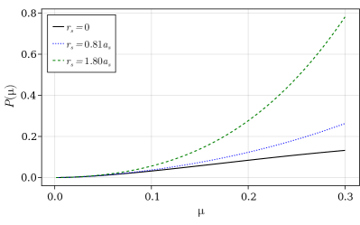
Figure 2: Zero-temperature pressure dependence on chemical potential, for three values of effective range $r_{s}$. Values are as computed in Ref. [14]. Dashed line is for case of Li-Li singlet state scattering, dotted line is for the case of Na-Na triplet state scattering, solid line is the prediction with the zero-range model. Length is in units of $a_{s}$, energy is in units of $\hbar^{2}/(ma_{s}^{2})$.

VIII Conclusions

We have shown a method for systematically relate, in generic spatial dimension $D$, the coefficients of the low momentum expansion of the interaction potential in terms of the s-wave scattering length and effective range, highlighting the two crucial assumptions that are present in the scheme, namely the s-wave and the on-shell approximations for the $T$-matrix equation. The on-shell approximation turns out to be an alternative to the assumption of a separable potential utilized in previous works [15]. We have explicitly calculated these relations in dimensions $D=1,\ 2,\ 3$ by using dimensional regularization, and we also discussed the discrepancy appearing in the literature for the expression of $g_{2}$ in the $D=3$ case, showing, using a different method, how the same results of Ref. [16, 17] can be obtained. Using this framework we have also obtained the finite-range correction to the zero-temperature pressure in a $D=2$ Bose system, which is in agreement with previous results [8]. It may be interesting to extend the proposed scheme for the case of atomic mixtures, which is getting increasing interest, or for atomic Josephson junctions in reduced spatial dimensions.

Appendix A: Legendre polynomials in arbitrary dimensions

Legendre polynomials in arbitrary dimension are defined, after fixing a direction, as the spherical hamonic of a rotational invariant homogeneous hamonic polynomial with respect to this direction. This defines them in a unique way [45]. We indicate them with the notation $P_{l}(\cdot)$ when the dimension is obvious. $P_{l}(\cdot)$ will in general depend on two versors, but due to the rotational invariance, it is only dependent on the angle in between through the inner product of versors. For every versor $\hat{\mathbf{x}}$ the following normalization condition holds

$$\int_{\mathbb{S}_{D}}d\omega\,P_{l}(\hat{\mathbf{x}}(\omega)\cdot\hat{\mathbf{y}})P_{l^{\prime}}(\hat{\mathbf{x}}(\omega)\cdot\hat{\mathbf{y}})=\dfrac{S_{D}}{N(D,l)}\delta_{ll^{\prime}},$$ (47)

where $\mathbb{S}_{D}$ is the unit spherical shell in $D$ dimensions, and $\hat{\mathbf{x}}$ is the corresponding versor. It is important to notice that it holds

$$P_{l}(1)= 1,$$ (48)

$$P_{l}(-1)= (-1)^{l}.$$ (49)

The above condition allows one to define the Legendre polynomial in the case $D=1$. In this case the angle can only assume values $0$ or $\pi$. Let $\hat{\mathbf{u}}^{+}$ be the versor in the positive direction, and $\hat{\mathbf{u}}^{-}$ in the negative direction. Integrating in the discrete measure, for $l=l^{\prime}$

$$\int_{\mathbb{S}^{1}}d\omega\,P_{l}^{2}(\hat{\mathbf{x}}(\omega)\cdot\hat{\mathbf{y}})=P_{l}^{2}(\hat{\mathbf{u}}^{+}\cdot\hat{\mathbf{y}})+P_{l}^{2}(\hat{\mathbf{u}}^{-}\cdot\hat{\mathbf{y}})=2.$$ (50)

in the last equality we used the fact that the argument of the Legendre polynomials can only assume values $\pm 1$, and the properties (48) and (49). Remembering that $S^{1}=2$, and using Eq. (47) we define the value of $N(1,l):=1$. By using the rotational symmetry, integral (47) can be evaluated separately in the angular variables that fixes the inner product. Let $\hat{\mathbf{x}}(\omega)\cdot\hat{\mathbf{y}}=t$,

$$\int_{\mathbb{S}_{D}}d\omega\,P_{l}(\hat{\mathbf{x}}(\omega)\cdot\hat{\mathbf{y}})P_{l^{\prime}}(\hat{\mathbf{x}}(\omega)\cdot\hat{\mathbf{y}})=$$

$$=S_{D-1}\int_{-1}^{1}P_{l}(t)P_{l^{\prime}}(t)(1-t^{2})^{(D-3)/2},$$

obtained by using the spherical hypersurface of radius $\sqrt{1-t^{2}}$ in $D$ dimensions: $S_{D}(1-t^{2})^{(D-3)/2}$ [45]. This normalization condition will be used in computing the partial wave expansion used in the s-wave approximation.

Finally, we point out that a similar generalization is available also for spherical Bessel functions, which are coefficient of the radial component of the partial wave expansion of the plane wave in general dimension $D$, are defined as [46, 45]

$$j_{l,D}(z)=\Gamma\left(\dfrac{D}{2}\right)\left(\dfrac{2}{z}\right)^{\frac{D}{2}-1}J_{l+\frac{D}{2}-1}(z)$$ (51)

where $J_{\alpha}$ is the Bessel J function of index $\alpha$, that can be rational.

Appendix B: Connection between s-wave and Fourier transform

As explained in the Introduction, the representations in momentum space of the matrix element of the operators $\hat{T}$ and $\hat{V}$ take the form of Fourier transforms calculated in the difference between the wavevectors. Let us focus on the operator $\hat{V}$, since the treatment of the operator $\hat{T}$ is identical. The Fourier transform is denoted by $\tilde{V}(\textbf{k}-\textbf{k}^{\prime})$,

$$V_{\textbf{k}\textbf{k}^{\prime}}=\dfrac{\tilde{V}(\textbf{k}-\textbf{k}^{\prime})}{(2\pi)^{D}}=\dfrac{1}{(2\pi)^{D}}\int d^{D}\textbf{r}\ V(r)\ e^{-i(\textbf{k}-\textbf{k}^{\prime})\cdot\textbf{r}},$$ (52)

In the hypothesis $|\textbf{k}|=|\textbf{k}^{\prime}|=k$, the difference vector can be expressed as

$$\textbf{k}-\textbf{k}^{\prime}=2k\sin\left(\theta/2\right)\hat{\textbf{u}},$$ (53)

where $\hat{\textbf{u}}$ is the versor of the difference, and $\theta$ the angle between the wavevectors. Clearly, for $D=1$ the angle $\theta$ has only two values: $\theta=0$ and $\theta=\pi$. It follows that the expression $\tilde{V}(\textbf{k}-\textbf{k}^{\prime})$ only depends on $k$ and $\theta$, so we refer to this quantity with the notation $\tilde{V}(2k\sin(\theta/2))={\color[rgb]{0,0,0}{\tilde{V}}({\bf k}-{\bf k}^{\prime})}$.

By using the standard expansion in partial waves, i.e. the Fourier-Legendre series, we can write

$$\tilde{V}(2k\sin(\theta/2))=\sum_{l=0}^{\infty}V_{l}(k)(2l+1)P_{l}(\cos(\theta)),$$ (54)

where $P_{l}(x)$ are Legendre polynomials, that satisfy the orthogonality relation [47]

$$\int_{-1}^{1}dx\ P_{l}(x)P_{l^{\prime}}(x)=\dfrac{2}{2l+1}\delta_{l,l^{\prime}}\;.$$ (55)

As a direct consequence of the Fourier-Legendre expansion one can compute the expansion coefficients via integration. These integrals are convergent for potentials that are square summable (Fischer-Riesz theorem). Explicit examples of potentials that satisfy this condition are discussed, for instance, in Refs. [3, 48]. In 3D and 2D, the integration is simply

$$V_{l}(k)={1\over 2}\int_{0}^{\pi}d\theta\ {\tilde{V}}(2k\sin(\theta/2))\ \sin(\theta)\ P_{l}(\cos(\theta))\;.$$ (56)

The s-wave case, i.e. $l=0$, gives exactly Eq. (11) because $P_{0}(x)=1$. However, in 1D the set of angles that $\theta$ can assume is discrete, containing only in $0$ and $\pi$. The same integral can be evaluated in a discrete measure giving

$$V_{l}(k)=\dfrac{1}{2}\left(\tilde{V}(0)+(-1)^{l}\tilde{V}(2k)\right)\;.$$ (57)

Notice that the first term of the expansion is the even part of $\tilde{V}$ with respect to the variable $\theta$ centered in $\pi/2$. Independently of the dimension D, the relationships $g_{0}={\tilde{g}}_{0}$ and $g_{2}=2{\tilde{g}}_{2}$ are verified.

References

- [1] A. Leggett, Quantum Liquids: Bose-condensation and Cooper pairing in condensed matter systems (Oxford Univ. Press, 2006).
- [2] L. Pitaevskii and S. Stringari, Bose-Einstein Condensation and Superfludity (Oxford Univ. Press, 2016).
- [3] H. T. C. Stoof, K. B. Gubbels, and D. B. M. Dickerscheid, Ultracold Quantum Fields (Springer, 2009).
- [4] A. Cappellaro and L. Salasnich, Thermal field theory of bosonic gases with finite-range effective interaction, Phys. Rev. A 95, 033627 (2017).
- [5] A. Cappellaro and L. Salasnich, Finite-range corrections to the thermodynamics of the one-dimensional Bose gas, Phys. Rev. A 96, 063610 (2017).
- [6] L. Salasnich, Nonuniversal Equation of State of the Two-Dimensional Bose Gas, Phys. Rev. Lett. 118, 130402 (2017).
- [7] S. R. Beane, Ground-state energy of the interacting Bose gas in two dimensions: An explicit construction, Phys. Rev. A 82, 063610 (2010).
- [8] S. R. Beane, Effective-range corrections to the ground state energy of the weakly-interacting Bose gas in two dimensions, Eur. Phys. J. D 72, 55 (2018).
- [9] J. J. García-Ripoll, V. V. Konotop, B. Malomed, and V. M. Pérez-García, A quasi-local Gross–Pitaevskii equation for attractive Bose–Einstein condensates, Math. Comput. Simul. 62, 21 (2003).
- [10] H. Fu, Y. Wang, and B. Gao, Beyond the Fermi pseudopotential: A modified Gross-Pitaevskii equation, Phys. Rev. A 67, 053612 (2003).
- [11] F. Sgarlata, G. Mazzarella, and L. Salasnich, Effective-range signatures in quasi-1D matter waves: sound velocity and solitons, J. Phys. B 48, 115301 (2015).
- [12] S. Giorgini, J. Boronat, and J. Casulleras, Ground state of a homogeneous Bose gas: A diffusion Monte Carlo calculation, Phys. Rev. A 60, 5129 (1999).
- [13] V. Cikojevi ć, L. V. Markić, G. E. Astrakharchik, and J. Boronat, Universality in ultradilute liquid Bose-Bose mixtures, Phys. Rev. A 99, 023618 (2019).
- [14] V. V. Flambaum, G. F. Gribakin, and C. Harabati, Analytical calculation of cold-atom scattering, Phys. Rev. A 59, 1998 (1999).
- [15] D. Phillips, S. Beane, and T. Cohen, Nonperturbative regularization and renormalization: Simple examples from nonrelativistic quantum mechanics, Ann. Phys. 263, 255 (1998).
- [16] H. W. Hammer and R. J. Furnstahl, Effective field theory for dilute Fermi systems, Nucl. Phys. A 678, 277 (2000).
- [17] E. Braaten, H.-W. Hammer, and S. Hermans, Nonuniversal effects in the homogeneous Bose gas, Phys. Rev. A 63, 063609 (2001).
- [18] S. Beane, G. Bertaina, R. C. Farrell, and W. Marshall, Toward precision Fermi liquid theory in flatland, preprint arXiv:2212.05177 (2022).
- [19] U. van Kolck, Effective field theory of short-range forces, Nucl. Phys. A 645, 273 (1999).
- [20] S. R. Beane and R. C. Farrell, Symmetries of the Nucleon–Nucleon S-Matrix and Effective Field Theory Expansions, Few-Body Syst. 63, 45 (2022).
- [21] D. B. Kaplan, M. J. Savage, and M. B. Wise, Two nucleon systems from effective field theory, Nucl. Phys. B 534, 329 (1998).
- [22] M. C. Birse, J. A. McGovern and K. G. Richardson, A renormalisation-group treatment of two-body scattering, Phys. Lett. B 464, 169 (1999).
- [23] D. B. Kaplan, M. J. Savage and M. B. Wise, Nucleon-nucleon scattering from effective field theory, Nuc. Phys. B 478, 629 (1996).
- [24] A. Collin, P. Massignan, and C. Pethick, Energy dependent effective interactions for dilute many-body systems, Phys. Rev. A 75, 013615 (2007).
- [25] H. Veksler, S. Fishman, and W. Ketterle, Simple model for interactions and corrections to the Gross-Pitaevskii equation, Phys. Rev. A 90, 023620 (2014).
- [26] R. Roth and H. Feldmeier, Effective s-and p-wave contact interactions in trapped degenerate fermi gases, Phys. Rev. A 64, 043603 (2001).
- [27] R. G. Newton, Scattering Theory of Waves and Particles (Springer-Verlag New York, 1982).
- [28] H. P. Noyes, New Nonsingular Integral Equation for Two Particle Scattering, Phys. Rev. Lett. 15, 538 (1965).
- [29] K. L. Kowalski, Off-Shell Equations for Two-Particle Scattering, Phys. Rev. Lett. 15, 798 (1965).
- [30] J. Sakurai and J. Napolitano, Modern Quantum Mechanics (Cambridge Univ. Press, 2017).
- [31] L. S. Rodberg and M. Thaler, Introduction to the Quantum Theory of Scattering (Academic Press, 1970).
- [32] A. M. J. Schakel, Boulevard of Broken Symmetries (World Scientific, 2008).
- [33] L. Salasnich and F. Toigo, Zero-point energy of ultracold atoms, Phys. Rep. 640, 1 (2016).
- [34] E. Zeidler, Quantum Field Theory II: Quantum Electrodynamics: A Bridge between Mathematicians and Physicists (Springer Science & Business Media, 2008).
- [35] V. E. Barlette, M. M. Leite, and S. K. Adhikari, Quantum scattering in one dimension, Eur. J. Phys. 21, 435 (2000).
- [36] V. E. Barlette, M. M. Leite, and S. K. Adhikari, Integral equations of scattering in one dimension, Am. J. Phys. 69, 1010 (2001).
- [37] S. K. Adhikari, Quantum scattering in two dimensions, Am. J. Phys. 54, 362 (1986).
- [38] N. N. Khuri, A. Martin, J.-M. Richard, and T. T. Wu, Low-energy potential scattering in two and three dimensions, J. Math. Phys. 50, 072105 (2009).
- [39] Y. Castin, Simple theoretical tools for low dimension Bose gases, J. Phys. IV France 116, 89 (2004).
- [40] G. Astrakharchik, J. Boronat, J. Casulleras, I. Kurbakov, and Y. E. Lozovik, Equation of state of a weakly interacting two-dimensional bose gas studied at zero temperature by means of quantum monte carlo methods, Phys. Rev. A 79, 051602 (2009).
- [41] A. Tononi, A. Cappellaro, and L. Salasnich, Condensation and superfluidity of dilute Bose gases with finite range interaction, New J. Phys. 20, 125007 (2018).
- [42] A. Tononi, Zero-Temperature Equation of State of a Two-Dimensional Bosonic Quantum Fluid with Finite Range Interaction, Cond. Matt. 4, 20 (2019).
- [43] C. Mora and Y. Castin, Extension of Bogoliubov theory to quasicondensates, Phys. Rev. A 67, 053615 (2003).
- [44] C. Mora and Y. Castin, Ground State Energy of the Two-Dimensional Weakly Interacting Bose Gas: First Correction Beyond Bogoliubov Theory, Phys. Rev. Lett. 102, 180404 (2009).
- [45] H. Hochstadt, The Functions of Mathematical Physics (Courier Corporation, 2012).
- [46] H. T. C. Stoof, L. P. H. de Goey, W. M. H. M. Rovers, P. S. M. Kop Jansen, and B. J. Verhaar, Nonsingular integral equation for two-body scattering and applications in two and three dimensions, Phys. Rev. A 38, 1248 (1988).
- [47] F. W. J. Olver, D. W. Lozier, R. F. Boisvert, and C. W. Clark, NIST handbook of mathematical functions (Cambridge Univ. Press, 2010).
- [48] J. Pera and J. Boronat, Low-energy scattering parameters: A theoretical derivation of the effective range and scattering length for arbitrary angular momentum, Am. J. Phys. 91, 90 (2023).