Topological Mixed Valence Model for Twisted Bilayer Graphene

Abstract

Song and Bernevig (SB) have recently proposed a faithful reformulation of the physics of magic angle twisted bilayer graphene (MATBG) as a topological heavy fermion problem, involving the hybridization of flat band f-electrons with a topological band of conduction electrons. Here we explore the consequences of this analogy, using it to reformulate the SB model as a mixed valence model for twisted bilayer graphene. We show how the interaction with the conduction sea behaves as a U(8) Kondo Lattice at high energies and a U(4) Kondo lattice at low energies. One of the robust consequences of the model, is the prediction that underlying hybridization scale of the mixed valent model and the width of the upper and lower Hubbard bands will scale linearly with energy. We also find that the bare hybridization $\gamma_{0}$ predicted by the SB model is too large to account for the observed local moment behavior at large filling factor, leading us to suggest that the bare hybridization is renormalized by the soft polaronic response of the underlying graphene.

I Introduction

The discovery of magic angle twisted bilayer graphene (MATBG), developing flat bands at “magic angles”[1, 2, 3, 4, 5, 6], has opened a new avenue for the exploration of quantum materials. At integral filling, novel spin and valley polarized [7, 8, 9, 10, 11] Mott insulators develop, which on doping transform into strange metals [12, 13, 14, 15, 16, 17, 18, 19, 20] and novel superconductors [21, 4], all of which have been a subject of intense theoretical study [22, 23, 24, 25, 26, 27, 28, 29, 30, 31, 32, 33, 34, 35, 36, 37, 38, 39, 40, 41]. It is as if, by tuning the voltage, one can explore a family of compounds along an entire row of the periodic table.

Various experiments suggest that electrons localized in the moiré hexagons of MATBG resemble quantum dots [42, 43], forming localized moments with valley and spin degeneracy near integer filling. This evidence includes the lifting of spin/valley degeneracy observed in Landau fans,[44] a field-tunable excess electronic entropy at integer filling $\nu$[45] and the appearance of upper and lower Hubbard band-like features in scanning tunneling microscopy measurements[46]. While the Bistritzer MacDonald [2] model for magic angle graphene, provides an accurate description of the plane-wave single-particle physics, the presence of local moments, governed by short-range Coulomb interactions underlines the importance of developing a real-space description of the physics, whilst taking the topology of the system into account [47, 48, 49, 50, 51, 52, 53, 54, 55, 56, 57].

A recent theory by Song and Bernevig (SB)[58] describes TBG as a topological heavy fermion problem [59]: they find, rather remarkably, that the moiré potential of TBG focuses the low energy electron waves into Wannier states that are tightly localized at the center of each moiré hexagon; the hybridization of these flat-band (“f”) Wannier-states with a topological conduction (“c”) band captures the essential mirror, time reversal and particle-hole symmetries of the Bistritzer-Macdonald model. The SB model establishes the correct band symmetries at the $\Gamma_{M}$ and $M_{M}$ points of the Brillouin zone, correctly giving rise to a pair of Dirac cones of the same chirality at the $K_{M}$ points of each valley. The symmetry anomaly of the $C_{2z}T$ and particle-hole symmetries $P$, responsible for the Dirac cones, is reproduced by a quadratic conduction band touching at $\Gamma_{M}$ in the conduction band: when hybridization is turned on, this anomaly is injected into the f-electron band.

In this paper, we build on early work establishing a Kondo lattice model for MATBG [60, 61, 62, 63]. We explore the consequences of the SB approach, examining the effects of valence fluctuations of well-localized f-states within a topological conduction band. The localized heavy fermions carry spin ($\sigma=\pm 1$) - valley ($\eta=\pm 1$) and orbital ($\alpha=\pm 1$) quantum numbers, forming an eight-fold degenerate multiplet that becomes mobile through the effects of valence fluctuations into a topological conduction band.

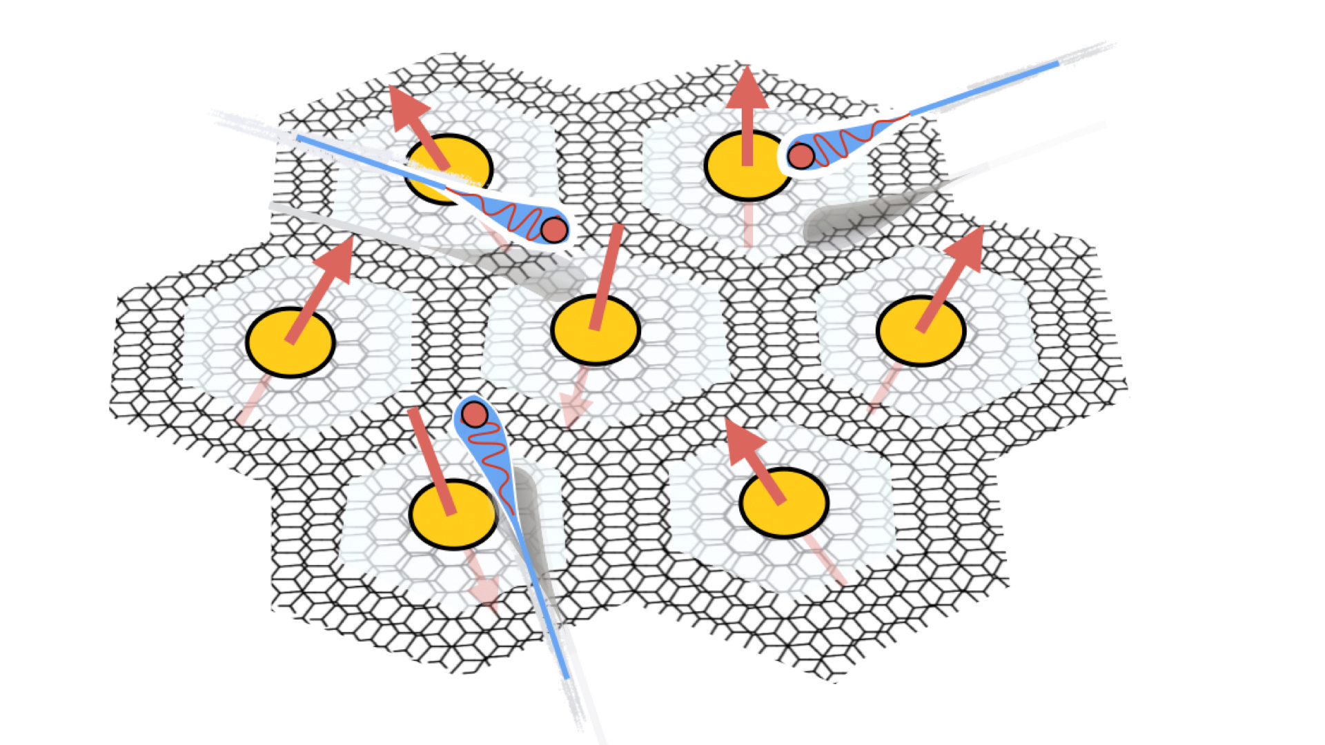
Figure 1: Hexagonal lattice of exponentially localized Wannier $f$-states (red) on each Moiré A-A site submerged in a sea of topological relativistic $c$-electrons (blue).

We consider the relevant energy scales from a moiré impurity model, bringing out the differences between gate tuned MATBG and traditional heavy fermion materials [64, 65, 66, 67, 68, 69, 70, 71]. One of the key differences with heavy fermion materials, is that the f-states in MATBG do not involve an ionic potential well that progressively deepens with atomic number or filling: the only way to dope the f-states away from neutrality is to raise the chemical potential of all electrons by changing a back-gate potential. This causes the conduction density of states accessible to the f-states to change rapidly as a function of filling, drastically altering the Kondo temperature. We estimate the doping dependence of the Kondo temperature, using a Doniach criterion [72, 73] to show that in the vicinity of integer filling, valley-spin magnetism will become stable, with quantum phase transitions into a heavy Fermi liquid which flank the valley-spin magnetic phases.

II Song Bernevig Model

The one-particle Hamiltonian of the SB model

$$H_{0}=H_{c}+H_{fc},$$ (1)

hybridizes exponentially localized Wannier $f$-electron states centered on the moiré A-A sites with topological conduction electrons defined by the Hamiltonian

$$H_{c} = \sum_{\begin{subarray}{c}|\textbf{k}|<\Lambda_{c}\\ a,a^{\prime}\eta\sigma\end{subarray}}c^{\dagger}_{\textbf{k}a\eta\sigma}\mathcal{H}_{aa^{\prime}}^{\left(\eta\right)}\left(\textbf{k}\right)c_{\textbf{k}a^{\prime}\eta\sigma}.$$ (2)

Here $c^{\dagger}_{{\textbf{k}}a\eta\sigma}$ creates a conduction electron with orbital, valley and spin quantum numbers $a\in(1,4)$, $\nu=\pm$ and $\sigma=\pm 1$ respectively. The orbital matrix

(3)

describes the mixing between the four orbitals in each valley $\eta$. The off-diagonal terms give rise to an asymptotically linear dispersion with velocity $v_{\star}$, where the Pauli matrices $\alpha_{\mu}\equiv(\alpha_{0},\vec{\alpha})$ ($\mu=0,3$) act on the two dimensional blocks. The first two entries of the matrix ($a=1,2$) refer to electrons with $\Gamma_{3}$ symmetry at the $\Gamma_{M}$, point ${\textbf{k}}=0$, while the lower block-diagonal $a=(3,4)$ describes two orbitals of $\Gamma_{1}$ and $\Gamma_{2}$ symmetry, split by a mass $M$.

$H_{c}$ gives rise to four bands with a four-fold spin-valley degeneracy at each k. The low energy dispersion is quadratic at $\Gamma_{M}$ and becomes relativistic $|E|\sim v_{\star}k$ at energies $|E|\gtrsim M$, with a bandwidth $D\sim v_{\star}K_{\theta}$. The single-particle model for TBG in each valley has a symmetry anomaly in the $C_{2z}T$ and particle-hole $P$ symmetries, corresponding to two Dirac cones at the Fermi-level with the same chirality. Since the local orbitals are topologically trivial, the unhybridized conduction electron band-structure carries the symmetry anomaly.

The hybridization between the conduction sea and $f$ electrons at each moiré A-A site R is described by

$$H_{fc} = \gamma_{0}\sum_{\textbf{R}\alpha a\eta\sigma}\left(f^{\dagger}_{\textbf{R}\alpha\eta\sigma}c_{\textbf{R}\alpha\eta\sigma}+\text{h.c.}\right)$$ (4)

and $H_{cf}=H_{fc}^{\dagger}$. Here $f^{\dagger}_{{\textbf{R}}\alpha\eta}$ creates an f-electron with orbital character $\alpha=1,2$, valley and spin quantum numbers $\eta$ and $\sigma$. The total degeneracy of the bare f-states is thus $2N_{f}=8$. $c^{\dagger}_{{\textbf{R}}\alpha\eta}$ creates a un-normalizable, non-exponentially localized Wannier state centered at R for the c-electron with the same quantum numbers and is related to the normalizable continuum $c^{\dagger}_{{\textbf{k}}a\eta\sigma}$ states as

$$c_{{\textbf{R}}\alpha\eta\sigma}=\frac{1}{\sqrt{N_{s}}}\sum_{\begin{subarray}{c}{{\textbf{k}}},{\bf G},a\\ |{\textbf{k}}+{\bf G}|<\Lambda_{c}\end{subarray}}e^{i{\textbf{k}}\cdot{\textbf{R}}}[\phi^{(\eta)}({\textbf{k}}+{\bf G},\gamma_{0})]_{\alpha a}c_{{\textbf{k}}+{\bf G}a\eta\sigma}.$$ (5)

where the sum over all momenta has been divided up into a sum over reciprocal lattice vectors ${\bf G}$ of the moiré lattice and a sum over momentum k restricted to the first moiré Brillouin zone. The matrix form factor is

$$\phi^{\left(\eta\right)}\left(\textbf{k},\gamma_{0}\right)=e^{\frac{-k^{2}\xi^{2}}{2}}\begin{pmatrix}\alpha_{0}+a_{\star}\left(\eta k_{x}\alpha_{x}+k_{y}\alpha_{y}\right),&0_{2\times 2}\end{pmatrix},$$ (6)

where $\gamma_{0}$ and $a_{\star}$ set the magnitude and length scale of the hybridization and $\xi$ is a damping factor proportional to the real space spread of the localized f-Wannier states. Remarkably, the focusing effect of interference off the moiré potential produces Wannier states of size $\xi\sim a_{M}/5$, about a fifth of the moiré unit cell size $a_{M}$. The natural bandwidth of the free theory is given by $D\sim v_{\star}K_{\theta}$, but after hybridization, $M$ becomes the bandwidth of the moiré flat bands, while $\gamma_{0}$ is the gap to the higher energy bands. The approximate scales for the parameters in the SB model are [58] $D=v_{\star}K_{\theta}\approx 133$meV, $\gamma_{0}=-25$meV, $M=$3.7meV, $v_{\star}=-4.3$eVÅ, $K_{\theta}=0.031\hbox{\AA}^{-1}$, $a_{\star}=65$Å, and $\xi=0.225a_{M}=27$Å for the size of the Wannier states, which gives $\tilde{\xi}=\xi K_{\theta}=0.84$.

The non-interacting SB model reproduces the band-structure of the Bistritzer MacDonald model, giving rise to a central band of width $2M$, split-off by an energy $\gamma_{0}$ from the upper and lower bands. The central band can contain up to $8$ electrons, and in the non-interacting model, an applied chemical potential causes the band-structure to move rigidly, so that by changing the chemical potential $\mu$ over a range from $-M$ to $M$, the electron count per moiré unit cell can be tuned from 0 to 8.

III Qualitative Considerations

In this section, we consider the effect of interactions on the SB model, examining discuss the criteria for local moment formation. We then discuss the effects of adiabatically turning on the interactions, assuming that the ground-state remains a Fermi liquid. Finally, we consider the Doniach criterion for the stability of the heavy Fermi liquid. This involves a comparison of two interaction scales: the Kondo temperature [64], where local moments are perfectly screened by the conduction sea and the magnetic RKKY temperature [74, 75, 76], describing the strength of magnetic interactions between the local, mediated by the conduction c-electrons. The competition between the Kondo scale with the magnetic RKKY scale is expected to lead to a sequence of spin-valley magnetic and heavy Fermi liquid phases separated by quantum phase transitions. We depict the relevant energy scales for the formation of local moments and correlated phases as a function of filling in the Doniach phase diagram shown in Fig. (5).

Amongst the various electron interactions considered by SB, the largest is the on-site Coulomb repulsion $U_{0}$ between the $f$-electrons. A back-of-the envelope calculation using the Wannier radius $\xi=27\hbox{\AA}$ gives $U_{0}\sim e^{2}/(4\pi\epsilon_{0}\xi)\sim 53meV$, a number quite close to the value $U_{0}=60$meV estimated by SB. This large onsite interaction stabilizes integer occupations $Q$ of the f-states. While the various interactions between the $f$ and $c-$ electrons are comparable with $U$, we argue that the low density of conduction electrons in the model allows us to neglect these terms in a simplified discussion.

At neutrality, twisted bilayer graphene contains $4$ f-electrons in each moiré unit cell. An excess (or deficit) of

$$\nu_{0}=Q-4$$ (7)

f-electrons is accomplished by applying a gate voltage. The effective Hamiltonian of the system is an Anderson lattice model,

$$H=H_{0}-\mu\hat{N}+\frac{U}{2}\sum_{{\textbf{R}}}(n_{f{{\textbf{R}}}}-4)^{2},$$ (8)

where $\mu$ is the chemical potential provided to all electrons by the gate, $\hat{N}$ is the total electron count, relative to neutrality, $n_{f{\textbf{R}}}$ is the (instantaneous) number of f-electrons in a moiré unit cell at site R, while $U$ is the effective interaction between the f-electron. In practice $U$ may be smaller than bare value $U_{0}\sim 60$meV obtained from the Song Bernevig model, due to renormalization effects.

There are several energy scales we have to consider for the formation of local moments. The first we discuss is the ionization energy required to add or remove an electron into a single moiré AA-site “atom” with $n_{f{\textbf{R}}}=Q$ electrons. We show that the ionization energies are dependent on the on-site repulsion $U$ and the filling factor $\nu$ of the moiré AA-site “atom”. In the Anderson model, the hybridization and Coulomb interaction compete with one another. Local moments only form when the Coulomb scale exceeds the non-interacting resonance width of the f-electron bound state immersed in a sea of c-electrons.

III.1 Coulomb Blockade Physics

We begin by considering the unhybridized atomic limit of the Anderson model, given simply by

$$H_{A}({\textbf{R}})=\frac{U}{2}(n_{f{\textbf{R}}}-4)^{2}-\mu n_{f{\textbf{R}}},$$ (9)

where $n_{f{\textbf{R}}}-4$ is the deviation from neutrality. In a conventional heavy electron system, the neutrality point is determined by the atomic number of the rare earth ions, but in MATBG, the neutrality point is the same for all fillings of the lattice, and the filling of the f-state is determined by the chemical potential, which acts equally on both conduction and f-electrons. The stability of the quantum dot with charge $Q$ requires that the ionization energies

$$\Delta E^{Q}_{\pm}=E_{Q\pm 1}-E_{Q}=\frac{U}{2}\pm(U\nu_{0}-\mu)$$ (10)

are both positive. The energies $\pm\Delta E^{Q}_{\pm}$ describe the offset location for the upper and lower Hubbard peaks in the f-spectral function (Fig. 4), and requirement that both are positive restricts the chemical potential to lie in the range

$$\biggl{|}\mu-U\nu_{0}\biggr{|}<\frac{U}{2}$$ (11)

Thus to achieve a filling $\nu_{0}$, the chemical potential provided by the back-gate must be close to $U\nu_{0}$. For each unit increase in filling factor, the conduction band sinks down by an amount $U$.

At a finite temperature $T$, the local moment will remain stable against ionization provided

$$k_{B}T\leq U/2-|U\nu_{0}-\mu|$$ (12)

This defines a saw-toothed phase boundary for the region of local moment behavior, as shown in Fig. (2).

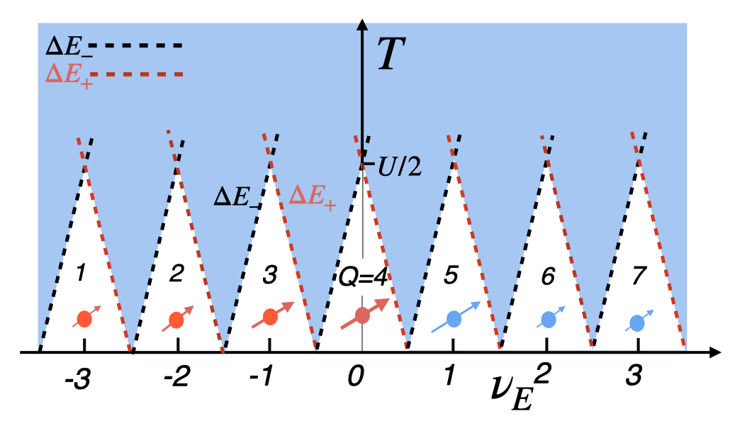
Figure 2: Sawtooth phase diagram for the “atomic limit” of MATBG, as a function of effective filling factor $\nu_{E}=\mu/U$. White regions denote a stable local moment with $Q$ f-electrons, bounded by the ionization energies $\Delta E_{\pm}$ for adding or removing one electron.

In the presence of a finite hybridization causes the f-valence to fluctuate through the virtual emission or absorption of electrons, $f^{Q}\rightleftharpoons f^{Q-1}+e^{-}$ and $e^{-}+f^{Q}\rightleftharpoons f^{Q+1}$. At energy scales below $U/2-U|\nu-\nu_{0}|$, the physics of the low-energy region are then described by a voltage-tuned “Kondo lattice”[77, 78].

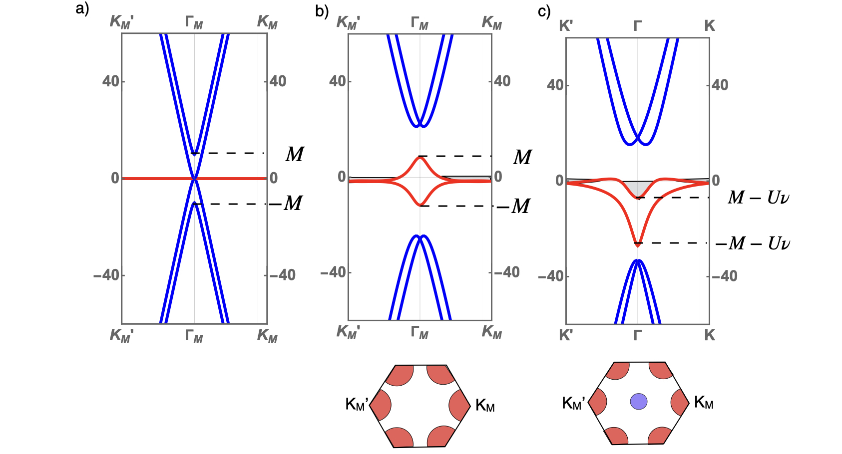
Figure 3: Schematic contrasting band-structure of MATBG in the SB model at fixed filling for a) zero hybridization b) finite hybridization, zero interaction, showing heavy Fermi surfaces at the $K_{M}$ points and c)finite interaction showing the downward movement of the conduction band by $U\nu$, and the appearance of a light electron pocket at the $\Gamma_{M}$ point.

III.2 Adiabatic Considerations: the Heavy Fermi Liquid

We now consider the effect of adiabatically turning on the Coulomb interaction. The non-interacting SB model describes a narrow band of f-electrons, with a linear Dirac dispersion of fixed chirality centered the $K_{M}$ points with a Dirac velocity $v_{D}$ (Derived in Appendix A). For instance, in the limit where $a_{\star}=0$

$$v_{D}\approx\left[3m(\gamma_{K}/D)^{2}\left(2+\tilde{\xi}^{2}\right)\right]v_{*}$$ (13)

where $m=M/D$, $D=v_{*}K_{\theta}$ and ${\gamma}_{K}=\gamma_{0}e^{-{\tilde{\xi}}^{2}/2}$ is the strength of the hybridization at the $K_{M}$ point. The approximate band-width of this flat band is given by $W=v_{D}K_{\theta}$.

On doping away from neutrality to a filling $\nu>0$, the Dirac points sink into the Fermi sea, producing two approximately circular Fermi surfaces of predominantly f-character, with four-fold valley spin symmetry, centered at each $K_{M}$ points, each of area $A_{FS}\sim\pi k_{F}^{2}$ area which satisfies Luttinger’s sum rule, which we can write as

$$8\frac{A_{FS}}{A_{M}}=\nu$$ (14)

where ${A}_{M}$ is the area of the moiré Brillouin zone (see Fig. 3b.) and $\nu$ the filling of the flat band. The non-interacting f-electrons thus form a Dirac sea of relativistic chiral fermions with a bandwidth of approximately $vDk_{F}$, occupying a fraction $\nu/8$ of the Brillouin zone. The SB model also predicts that at the $\Gamma_{M}$ point, the energy eigenvalues are $\epsilon_{\Gamma}=\left\{\pm M-\mu,\pm\gamma_{0}-\mu\right\}$, where those with energy $\pm M$ are entirely of conduction character, whereas those with energy $\pm\gamma_{0}-\mu$ are an equal admixture of f and topological conduction electrons. As a whole however, the flat band is predominantly of f-character, dominating the bulk properties.

Let us consider what happens when interactions are adiabatically introduced at constant filling factor $\nu$ to produce a Landau Fermi liquid. Now the f-states will renormalize with a Quasi-particle weight $Z_{f}$ characterizing the $K_{M}$ points of the Brillouin zone. So long as the ground-state remains a Fermi liquid, the Fermi surface area remains an adiabatic invariant, which will cause the f-states to remain pinned close to the Fermi energy, with energies $\epsilon_{{\textbf{k}}}=\lambda\pm v^{*}_{D}|{\textbf{k}}-{\bf K_{M}}|$, here $v^{*}=Z_{f}v_{D}$ is a renormalized Fermi velocity while in $\lambda\sim W^{*}=Z_{f}W$ is of order the renormalized band-width.

By contrast, the Coulomb blockade physics guarantees the chemical potential must take the value $\mu\sim U\nu$, so that the energy eigenvalues around the $\Gamma_{M}$ point will take the form

$$\epsilon_{\Gamma}=\biggl{(}\pm M-U\nu,-\frac{1}{2}U\nu\pm\sqrt{\left(\frac{U\nu}{2}\right)^{2}+Z_{f}(\gamma_{0})^{2}}\biggr{)}.$$ (15)

This produces a large distortion in the renormalized band-structure around the $\Gamma$ point. If we connect up the Dirac dispersion to the two points at $\pm M$, we see that the shape of the narrow band distorts on doping into a dove-shaped configuration for positive $\nu$, moustache-shaped for negative $\nu$. This strong renormalization effect is also expected to produce a second light Fermi surface at high doping, nestled around the $\Gamma_{M}$ point (see Fig. 3c. ).

III.3 Anderson Criterion

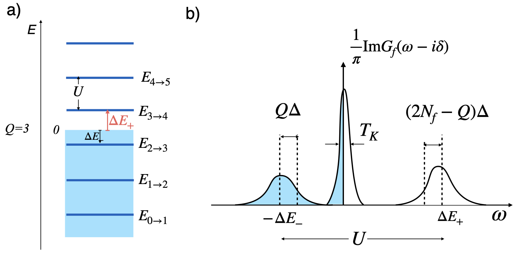
Figure 4: a) Energy level diagram showing the position of the Fermi energy relative to the f-level excitation energies for the case $Q=3$, $\nu_{0}=-1$. b) Spectral function for the f-state in an impurity model, showing upper and lower Hubbard resonances and the central Kondo resonance.

We now extract the key scales of the SB Anderson lattice by considering the corresponding impurity Anderson model, formed from a single moiré f-state embedded in a relativistic electron gas. This essential simplification can not describe the detailed effects of coherence that develop in the lattice, but it can provide us with a simple understanding of the key energy scales in the lattice.

The relativistic character of the conduction sea gives rise to a density of states per moiré per valley per spin, that is linear in energy at high energies. The density of states per spin per valley per orbital in the channel that hybridizes with the f-states is

$$\rho_{c}(E)=\frac{A}{D^{2}}\times\left\{\begin{array}[]{cc}|E|,&|E|>M\cr\cr\frac{1}{2}(|E|+M),&|E|<M.\end{array}\right.$$ (16)

where $A=2\pi/(3\sqrt{3})\approx 1.2$. In the presence of a chemical potential, this density of states shifts downwards in energy by an amount $\mu$, and now $\rho_{c}(E,\mu)=\rho_{c}(E+\mu)$.

If we ignore the effects of interaction, the hybridization width (half width at half maximum) of an isolated non-interacting Anderson impurity is given by

$$\Delta_{0}[\mu]=\pi\rho_{c}(\mu)\gamma_{0}^{2}$$ (17)

where $\gamma$ is the strength of the hybridization. It is instructive to compare $\Delta_{0}(0)$ at neutrality with the band-width $W=v_{D}K_{\theta}$ obtained in the SB band structure. From (13), we obtain

$$W=v_{D}K_{\theta}=3(1+(\xi K_{\theta})^{2})\left(\frac{\gamma_{K}}{D}\right)^{2}M\approx 2.5\left(\frac{\gamma_{0}}{D}\right)^{2}M,$$

while from (16), we obtain

$$\Delta_{0}(\mu=0)=\frac{\pi A}{2}\left(\frac{\gamma_{0}}{D}\right)^{2}M\approx 1.9\left(\frac{\gamma_{0}}{D}\right)^{2}M$$ (18)

so the two quantities are of comparable magnitude at neutrality. It is interesting to note that the hybridization entering into the flat band-width is the magnitude of the hybridization $\gamma_{K}=\gamma_{0}e^{-\xi^{2}K_{\theta}^{2}/2}\sim 0.7\gamma_{0}$ at the $K_{M}$ point where the f-excitations are concentrated. This comparison provides an important cross-check on our use of an equivalent impurity model to determine the key energy scales of the SB Anderson lattice model.

Now for a filling factor $\nu$, we expect a shift in the chemical potential $|\mu|\approx U|\nu|$, and since $U\gg M$, on doping away from neutrality, for $U|\nu|>M$, we expect the hybridization width and the flat band-width $W$ to both increase linearly with filling $\nu$. This robust observation, depending only on the linear density of states of the topological conduction electrons and the doping-dependent shift of the chemical potential is an important consequence of interactions in the SB model.

When the interactions are turned on, the f-spectral function splits into an upper and lower Hubbard peak at locations $E^{Q}_{+}$ and $-E^{Q}_{-}$, with a Kondo resonance in the center as shown in Fig. 4. The upper and lower resonances have a half-width of order $(2N_{f}-Q)\Delta_{0}$ and $Q\Delta_{0}$, where $2N_{f}=8$ for TBG. Well-defined local moment behavior then requires that the separation $U$ between the upper and lower Hubbard bands, is larger than their combined half-widths i.e

$$\Gamma_{0}=2N_{f}\Delta_{0}[\mu]\biggr{|}_{|\mu|=U|\nu|}=8\pi A\left(\frac{\gamma_{0}}{D}\right)^{2}U|\nu|\ll U.$$ (19)

We shall see that this is also the condition that the exponential factor in the Kondo temperature is smaller than one, see (28). Curiously, the strength of interaction $U$ factors out of this expression, implying that local moment formation is only expected for a chemical potential

$$|\nu|<\frac{1}{8\pi A}\left(\frac{D}{\gamma_{0}}\right)^{2},$$ (20)

an estimate that depends purely on the ratio of hybridization to bandwidth. With the hybridization $\gamma_{0}\approx 25$meV from Song-Bernevig, $D/\gamma_{0}\approx 5.2$, would imply that local moments would only form for $|\nu_{\text{eff}}|=|\mu/U|\lesssim 2/(\pi A)=0.9$. If we use the slightly smaller value of the hybridization at the $K_{M}$ point, $\gamma_{K}$, we obtain $|\nu|<1.25$.

Yet, there is considerable evidence of local moment behavior from entropy measurements and STM measurements even at a filling factor of $\nu=+3$[46, 45], suggesting a need for a substantially smaller hybridization. If we take for example, $\Gamma_{0}=U/4$, then this requires $\gamma\sim D/\sqrt{360}\approx 6.3$meV. This discrepancy between the SB value $\gamma_{0}\sim 25$meV and the value $\gamma$ required for local moment physics is concerning, and suggests that there may be an additional source of screening that lies outside the SB model. A likely candidates for this effect are the highly polarizable phonons of bilayer graphene In TBG the characteristic Debye frequency is considerably larger than the flat-band width: this region of parameter space is means that phonons respond adiabatically to valence fluctuations, giving rise to a polaronic renormalization effects. When an electron from the conduction sea tunnels into the tightly bound f-state, the greater electron density at the moiré AA-site pulls the surrounding carbon nuclei in, reducing the hybridization to

$$\gamma_{0}\rightarrow\gamma_{0}\exp{\left(-n_{ph}/2\right)}$$ (21)

where $n_{ph}$ is the number of phonons modes that are condensed by the breathing motion. To reduce the hybridization by a factor of would require the condensation of $n_{ph}\sim 3$ phonons. Such effects would likely lead to a strongly frequency and temperature dependent renormalization of $\gamma_{0}$ which lie beyond the scope of the current work. In the current work, we shall assume a renormalized value of $\gamma_{0}^{*}$ such that $\Gamma_{0}=U/4$ at $|\nu|=3$. The characteristic length scale of the hybridization $a_{\star}$ is approximately the distance between the moiré AB site and the AA site where the exponentially localized Wannier f-states reside. We expect $a_{\star}$ to remain approximately constant, even with the condensation of phonon modes.

III.4 Coqblin Schrieffer Transformation and the Kondo Temperature

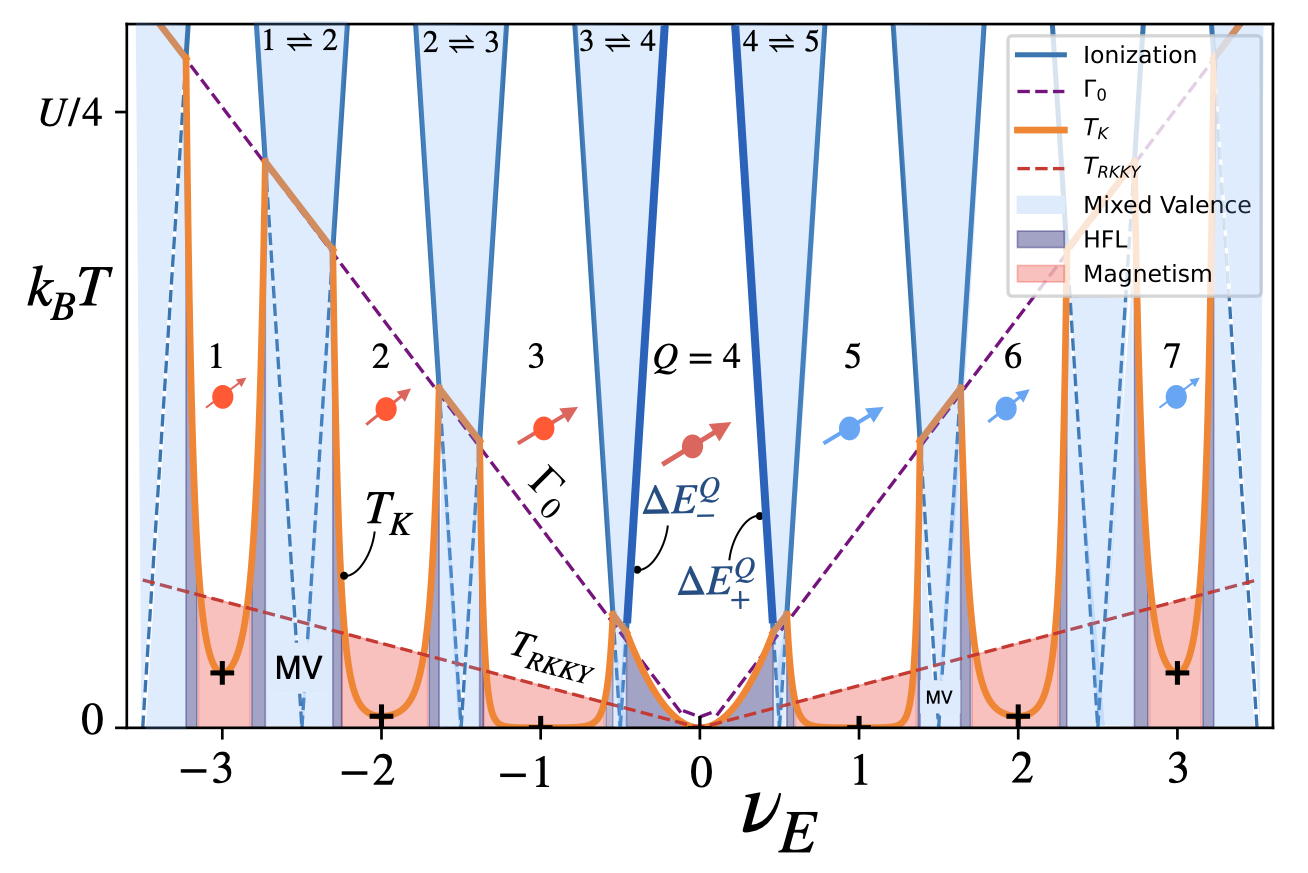
Figure 5: Proposed doping-temperature phase diagram for twisted bilayer graphene based on an impurity model for the f-states in MATBG. Here $\nu_{E}=\mu/U$ is the effective doping. The hybridization width $\Gamma_{0}[\nu]=2N_{f}\Delta_{0}[\mu]$ (purple dotted line) is an approximately linear function of doping. Ionization energies $\Delta E^{Q}_{\pm}$ are denoted by blue lines. Light blue regions are mixed valent. At temperatures smaller than the two ionization energies $E^{Q}_{\pm}$, (white regions), stable local moments develop. In the presence of hybridization, the criteria for Kondo physics is that resonance width $\Gamma_{0}=2N_{f}\Delta_{0}$, dotted purple line, is smaller than the ionization energies, blue lines, i.e $2N_{f}\Delta_{0}\ll{\rm min}(E^{Q}_{+},E^{Q}_{-})$. We have chosen $\Gamma_{0}(|\nu|=3)=U/4$, and $U=35$meV to allow for local moment physics at $\nu_{E}=3$. The Kondo temperature $T_{K}$, below which the f-states will develop coherence, is shown as an orange curve and the magnetic RKKY scale $T_{RKKY}$ as a dashed red line. Red regions denote valley-spin magnetic phases where $T_{RKKY}>T_{K}$. In the dark blue regions, where $T_{K}>T_{RKKY}$, a heavy Fermi liquid ground state is stabilized in which where each moiré $AA$-site coherently scatters the conduction electrons. The competition between $T_{K}$ and $T_{RKKY}$ leads to a series of quantum phase transitions [73, 72] straddling each integer filling factor. A weakly coupled Song-Bernevig phase develops at low temperatures in the blue regions.

The resulting low energy effective Hamiltonian

$$H_{K}=\sum_{\scriptsize{v_{\star}|{\textbf{k}}|<D}}c^{\dagger}_{{\textbf{k}}}\mathcal{H}\left({\textbf{k}}\right)c_{{\textbf{k}}}+J_{\text{eff}}\sum_{\textbf{R}BB^{\prime}}\tilde{c}^{\dagger}_{\textbf{R}B}\tilde{c}_{\textbf{R}B^{\prime}}S_{BB^{\prime}}\left(\textbf{R}\right)$$ (22)

is a Topological Kondo lattice model. Here $B\equiv\left(\alpha\eta\sigma\right)_{2}\equiv 1,2\ldots 8$ is the $SU(8)$ index written in binary and

$$S_{BB^{\prime}}({\textbf{R}})=f^{\dagger}_{{\textbf{R}}B}f_{{\textbf{R}}B^{\prime}}-\frac{Q}{2N_{f}}\delta_{BB^{\prime}}$$ (23)

is the SU (8) spin operator. Lastly,

$$\tilde{c}_{\textbf{R}B}=\frac{1}{\sqrt{N_{s}}}\sum_{\begin{subarray}{c}|\textbf{k}|<\Lambda_{c}\\ \textbf{R}\alpha a\eta\end{subarray}}\phi^{\left(\eta\right)}_{\alpha a}(\textbf{k})c_{\textbf{k}a\eta s}e^{i\textbf{k}\cdot\textbf{R}},$$ (24)

creates a spatially extended $\Gamma_{3}$ conduction electron state, centered (rather than localized) at R with quantum numbers $B$. The strength of the effective Kondo interaction

$$J_{\text{eff}}=\sum_{\pm}\frac{(\gamma^{*}_{0})^{2}}{\Delta E_{Q\rightarrow Q\pm 1}}=\frac{4(\gamma^{*}_{0})^{2}}{U}\ F[\frac{\mu}{U}-\nu_{0}]$$ (25)

where $F[x]=1/(1-(2x)^{2})$. Notice that the multiplying factor $F=1$ is unity at integral filling, ($\nu_{\text{eff}}=\mu/U=\nu_{0}$).

An emergent crossover temperature from Kondo physics is the Kondo temperature $T_{K}$ at which the local moments at each moiré AA-site is screened by the conduction c-electrons, forming a Kondo singlet at each moiré AA-site. The Kondo temperature $T_{K}$ at integer fillings $\nu_{0}$ can be estimated as

$$T_{K}[\nu_{0}] \sim \Lambda\exp{\left(-\frac{1}{(8J_{\text{eff}}\rho_{c})}\right)}$$ (26)

$$\approx \Lambda\exp{\left(-\frac{U\pi(1-4(\mu/U-\nu_{0})^{2})}{32\Delta_{0}[\mu]}\right)}\Biggl{|}_{\mu=U\nu_{0}}$$ (27)

where $\Lambda$ is an appropriate cutoff. A more careful calculation reveals that $\Lambda=M$ at neutrality, and $U/2$ at $\nu_{0}\neq 0$, giving

$$T_{K}[\nu_{0}]=\begin{cases}M\exp{\left(-\frac{1}{16A}\frac{U}{M}\left(\frac{D}{\gamma^{*}_{0}}\right)^{2}\right)},\ \ \ (\nu_{0}=0),\\ \frac{U}{2}\exp{\left(-\frac{1}{32A\nu_{0}}\left(\frac{D}{\gamma^{*}_{0}}\right)^{2}\right)},\ \hskip 10.00002pt(\nu_{0}\neq 0).\end{cases}$$ (28)

Note that the size of $U$ disappears from the exponent for non-zero $\nu_{0}$, and that the condition that $T_{K}\ll U/2$ at finite $\nu_{0}$ is equivalent to condition (20) considered in section III.3. In Fig. (5), we interpolate the Kondo temperature, shown in green, between the non-interacting resonance width $\Delta_{0}[U\nu]$ and $T_{K}[\nu_{0}]$.

III.5 Magnetic RKKY Temperature

The magnetic moments at each moiré AA-site induces a cloud of Friedel oscillations in the spin-valley density with a magnetization profile that couples to neighboring local moments via a long-range RKKY interaction [74, 75, 76]. The RKKY interaction drives long-range spin-valley magnetic ordering and we can estimate the RKKY magnetic energy scale $T_{RKKY}$ to be

$$T_{RKKY}[\mu]\sim 8J^{2}\rho_{c}(\mu)=\frac{8AD^{2}}{U}\left(\frac{2\gamma^{*}_{0}}{D}\right)^{4}\frac{\mu}{U},$$ (29)

where $J=4(\gamma^{*}_{0})^{2}/U$ is the characteristic Kondo scale. We depict the RKKY temperature as the red dashed line in Fig. (5).

III.6 Doniach Criterion

In the regimes near integer filling, where $T_{RKKY}>T_{K}$, there would be a valley-spin magnetic phase depicted as highlighted red in Fig. (5). Away from integer filling but in the regions where local moments can form, the Kondo temperature can be larger than the magnetic energy scale $T_{RKKY}$, $T_{K}>T_{RKKY}$. In these regions of the phase diagram, a heavy Fermi liquid ground state is stabilized, shown as highlighted dark blue in Fig. (5), and every $AA$-site coherently scatters conduction electrons. Consequently, the competition of the Kondo scale and the magnetic RKKY scale leads to a series of quantum phase transitions straddling each integer filling factors.

The physics in the regions outside where local moments are stabilized is governed by a weakly coupled Song-Bernevig model, leading to a Fermi liquid.

IV Mixed Valence Model

We now outline a theory that enables us to develop a mean-field picture of the valence fluctuations and Kondo effect in MATBG. At an energy scale greater than $U/2$, the valence of the moire ion begins to fluctuate $Q\rightleftharpoons Q\pm 1$ with excitation energies $\Delta E_{\pm}=U/2\pm(U\nu_{0}-\mu)$ and the Moire f-state can no longer be simply described by local moments. We can treat the fluctuations as vector bosons [79, 80]

$$w\equiv\begin{pmatrix}t\\ b\end{pmatrix}$$ (30)

which describe the addition and removal of charge in the Wannier localized f-state. The physical states are:

$$|f^{Q}\rangle = \prod_{j=1,Q}f^{\dagger}_{\sigma_{j}}|0\rangle,\qquad$$ (31)

$$|f^{Q-1}\rangle = b^{\dagger}\prod_{j=1,Q-1}f^{\dagger}_{\sigma_{j}}|0\rangle,$$ (32)

$$|f^{Q+1}\rangle = t^{\dagger}\prod_{j=1,Q+1}f^{\dagger}_{\sigma_{j}}|0\rangle,$$ (33)

subject to the constraint $n_{f}+n_{b}-n_{t}=Q$.

IV.1 Single Impurity Case

To develop the theory for the lattice, it is instructive to first consider the simplified case of a mixed valent impurity model with a $2N_{f}$ fold degeneracy. The action for a single impurity mixed valence model is

$$S=\int_{0}^{\beta}d\tau\left\{L_{c}+L_{f}+L_{b}+\gamma_{0}\sum_{{\textbf{k}},B}\left[c^{\dagger}_{{\textbf{k}}B}f_{B}(b^{\dagger}+t)+{\rm H.c}\right]\right\},$$ (34)

where

$$L_{c}=\sum_{{\textbf{k}},B}c_{{\textbf{k}}B}^{\dagger}(\partial_{\tau}+\epsilon_{{\textbf{k}}}-\mu)c_{{\textbf{k}}B},$$ (35)

and

$$L_{f}=\sum_{B}f^{\dagger}_{B}(\partial_{\tau}+\lambda)f_{B}-(\lambda+\mu)Q,$$ (36)

describes the unhybridized fermions and

$$L_{b}=b^{\dagger}(\partial_{\tau}+\Delta E_{-}+\lambda)b+t^{\dagger}(\partial_{\tau}+\Delta E_{+}-\lambda)t,$$ (37)

describes the excitations into the upper and lower Hubbard bands, where $\Delta E_{\pm}=U/2\pm(U\nu_{0}-\mu)$. The integration over the $\lambda$ degree of freedom imposes the constraint $n_{f}+n_{b}-n_{t}=Q$. Introducing the symmetric and antisymmetric boson fields, $s=(b+t^{\dagger})/{\sqrt{2}}$, $\delta=(b-t^{\dagger})/{\sqrt{2}}$, the action becomes

$$S=\int_{0}^{\beta}d\tau\left\{L_{c}+L_{f}+L_{s}+\sqrt{2}\gamma^{*}_{0}\sum_{{\textbf{k}},B}\left[c^{\dagger}_{{\textbf{k}}B}f_{B}s+{\rm H.c}\right]\right\},$$ (38)

where now

$$L_{s}=\frac{U}{2}\left[s^{\dagger}s+\delta^{\dagger}\delta\right]+s^{\dagger}(\lambda+\mu-U\nu_{0}+\partial_{\tau})\delta+\delta^{\dagger}(\lambda+\mu-U\nu_{0}+\partial_{\tau})s.$$ (39)

Notice that the antisymmetric $\delta$ field decouples from the fermions and can be integrated out to then obtain

$$S=\int_{0}^{\beta}d\tau\left\{L_{c}+L_{f}+\sum_{{\textbf{k}},B}\left[c^{\dagger}_{{\textbf{k}}B}f_{B}s+{\rm H.c}\right]+\frac{1}{J}s^{\dagger}\left[1-\left(\frac{\lambda+\mu-U\nu_{0}+\partial_{\tau}}{U/2}\right)^{2}\right]s\right\}$$ (40)

where we have rescaled $\sqrt{2}\gamma^{*}_{0}s\rightarrow s$ and introduced the Kondo coupling constant $J=4(\gamma^{*}_{0})^{2}/U$. The resulting action is remarkably similar to that of the Kondo lattice, but the frequency, $\lambda$ and $\mu$ inside the bosonic Lagrangian allows us to keep track of the dynamical valence fluctuations. Notice, that we can absorb the $-U\nu_{0}$ into a shift of the chemical potential, shifting $\mu\rightarrow\mu+U\nu_{0}$, but now this has the effect of shifting the conduction bands down in energy, so that our final action takes the form

$$S=\int_{0}^{\beta}d\tau\left\{{L}^{*}_{c}+L_{f}+\sum_{{\textbf{k}},B}\left[c^{\dagger}_{{\textbf{k}}B}f_{B}s^{\dagger}+{\rm H.c}\right]+\frac{1}{J}s^{\dagger}\left[1-\left(\frac{\lambda+\mu+\partial_{\tau}}{U/2}\right)^{2}\right]s\right\}$$ (41)

where now

$${L}^{*}_{c}=\sum_{{\textbf{k}},B}c_{{\textbf{k}}B}^{\dagger}(\partial_{\tau}+\epsilon_{{\textbf{k}}}-\mu-U\nu_{0})c_{{\textbf{k}}B}$$ (42)

describes the shifted conduction bands.

We can construct mean-field solutions by treating $\lambda$ and $s$ as constants, so that the mean-field action becomes

$$S=\int_{0}^{\beta}d\tau\left\{L^{*}_{c}+L_{f}+\sum_{{\textbf{k}},B}\left[c^{\dagger}_{{\textbf{k}}B}f_{B}s+{\rm H.c}\right]+\frac{|s|^{2}}{J}\left[1-\left(\frac{\lambda+\mu}{U/2}\right)^{2}\right]\right\}$$ (43)

We can identify

$$-\frac{\partial S}{\partial\mu}=N_{e}=N_{c}+Q+\frac{|s|^{2}}{(\gamma^{*}_{0})^{2}}\left(\frac{\lambda+\mu}{U/2}\right)$$ (44)

as the total charge while

$$\frac{\partial S}{\partial\lambda}=0=n_{f}-Q-\frac{|s|^{2}}{(\gamma^{*}_{0})^{2}}\left(\frac{\lambda+\mu}{U/2}\right)$$ (45)

as the constraint. The quantity

$$\frac{|s|^{2}}{(\gamma^{*}_{0})^{2}}\left(\frac{\lambda+\mu}{U/2}\right)=|t|^{2}-|b|^{2}$$ (46)

appearing on the right-hand side of these two expressions is identified as the correction to the f-charge density derived from valence fluctuations into the upper and lower Hubbard bands. We can combine (45) and (46) to obtain $N_{e}=N_{c}+n_{f}$.

V Mixed Valent Moiré Lattice

The procedure for developing a mean-field theory for TBGK follows the same lines as the above development. The lattice action is now

$$S=\int_{0}^{\beta}d\tau\left\{L_{c}+L_{f}+L_{b}+\gamma^{*}_{0}\sum_{{\textbf{R}},B}\left[c^{\dagger}_{{\textbf{R}}B}f_{{\textbf{R}}B}(b_{{\textbf{R}}}^{\dagger}+t_{{\textbf{R}}})+{\rm H.c}\right]\right\},$$ (47)

where

$$L_{c}=\sum_{{\textbf{k}},a,a\eta\sigma}c_{{\textbf{k}}a\eta\sigma}^{\dagger}(\partial_{\tau}+{\cal H}^{\eta}_{aa^{\prime}}({\textbf{k}})-\mu)c_{{\textbf{k}}a^{\prime}\eta\sigma}+\mu\langle N_{c}\rangle_{\nu=0},$$ (48)

here $\langle N_{c}\rangle_{\nu=0}$ is the number of conduction electrons at half filling and

$$L_{f}=\sum_{{\textbf{R}}}\left[f^{\dagger}_{{\textbf{R}}B}(\partial_{\tau}+\lambda_{{\textbf{R}}})f_{{\textbf{R}}B}-\lambda_{{\textbf{R}}}Q-\mu(Q-4)\right],$$ (49)

describes the unhybridized fermions and

$$L_{b}=\sum_{{\textbf{R}}}\left[b_{{\textbf{R}}}^{\dagger}(\partial_{\tau}+\Delta E_{-}+\lambda_{{\textbf{R}}})b_{{\textbf{R}}}+t_{{\textbf{R}}}^{\dagger}(\partial_{\tau}+\Delta E_{+}-\lambda_{{\textbf{R}}})t_{{\textbf{R}}}\right],$$ (50)

defines the valence fluctuations. Carrying out the same sequence of manipulations used in the single impurity, we obtain

$$S=\int_{0}^{\beta}d\tau\left\{{L}^{*}_{c}+L_{f}+\sum_{{\textbf{R}},B}\left[c^{\dagger}_{{\textbf{R}}B}f_{{\textbf{R}}B}s^{\dagger}_{{\textbf{R}}}+{\rm H.c}\right]+\frac{1}{J}\sum_{{\textbf{R}}}s_{{\textbf{R}}}^{\dagger}\left[1-\left(\frac{\lambda_{{\textbf{R}}}+\mu+\partial_{\tau}}{U/2}\right)^{2}\right]s_{{\textbf{R}}}\right\}$$ (51)

where now

$${L}^{*}_{c}=\sum_{{\textbf{k}},a,a^{\prime}\eta\sigma}c_{{\textbf{k}}a\eta\sigma}^{\dagger}(\partial_{\tau}+{\cal H}^{\eta}_{aa^{\prime}}({\textbf{k}})-\mu-U\nu_{0})c_{{\textbf{k}}a^{\prime}\eta\sigma}+(\mu+U\nu_{0})\langle N_{c}\rangle_{\nu=0},$$ (52)

describes the shifted conduction bands.

VI Mean-field Approach

Setting the $\lambda_{{\textbf{R}}}=\lambda$ and $s_{{\textbf{R}}}=\gamma$ in the above action, we obtain the following mean-field Hamiltonian takes the form

$$H_{\text{MF}}=\sum_{{\textbf{k}}\eta\sigma}\Psi^{\dagger}_{{\textbf{k}}\eta\sigma}\textbf{$\mathcal{H}$}^{\text{MF}}\left({\textbf{k}}\right)\Psi_{{\textbf{k}}\eta\sigma}+N_{s}\left(\frac{\bar{\gamma}\gamma}{J}\left[1-\left(\frac{\lambda+\mu}{U/2}\right)^{2}\right]-\mu\nu_{0}+(\mu+U\nu_{0})\langle N_{c}\rangle_{\nu=0}-\lambda Q\right),$$ (53)

where

$${\cal H}_{MF}({\textbf{k}})=\begin{pmatrix}\lambda\sigma_{0}&{\cal H}^{(\eta)}_{cf}[\bar{\gamma}]({\textbf{k}})&\dots&{\cal H}^{(\eta)}_{cf}[\bar{\gamma}]({\textbf{k}}+{\textbf{G}}_{n})\cr{\cal H}^{(\eta)}_{fc}[\gamma]({\textbf{k}})&{\cal H}^{(\eta)}_{c}({\textbf{k}})-(\mu+U\nu_{0}){\underline{1}}&0&0\cr\vdots&0&\ddots&0\cr{\cal H}^{(\eta)}_{fc}[\gamma]({\textbf{k}}+{\textbf{G}}_{n})&0&\dots&{\cal H}^{(\eta)}_{c}({\textbf{k}}+{\textbf{G}}_{n})-(\mu+U\nu_{0}){\underline{1}}\end{pmatrix}$$ (54)

describes the dispersion with renormalized hybridization strength $\gamma$, and $\Psi_{{\textbf{k}}\eta\sigma}=(f_{{\textbf{k}}1\eta\sigma},f_{{\textbf{k}}2\eta\sigma},c_{{\textbf{k}}1\eta\sigma},c_{{\textbf{k}}2\eta\sigma},c_{{\textbf{k}}3\eta\sigma},c_{{\textbf{k}}4\eta\sigma},c_{{\textbf{k}}+{\textbf{G}}_{1}1\eta\sigma},\dots,c_{{\textbf{k}}+{\textbf{G}}_{n}3\eta\sigma},c_{{\textbf{k}}+{\textbf{G}}_{n}4\eta\sigma})^{T}$ is a spinor combining the four conduction for each reciprocal lattice vector and two f-electron operators at each valley $\eta=\pm 1$ and spin $\sigma=\pm 1$. Notice that while $H_{MF}({\textbf{k}})$ commutes with the spin and valley quantum numbers, at general momentum it breaks the two-fold $\Gamma_{3}$ degeneracy down to a $N_{f}=4$ fold valley-spin degeneracy. The mean-field Free energy obtained by integrating out the fermions for a static configuration of the fields $(\gamma,\lambda)$, is then

$$F=-N_{f}T\sum_{{\textbf{k}},i\omega_{n}}{\rm Tr}{\rm\ ln}(-i\omega_{n}+{\cal H}_{MF}({\textbf{k}}))+N_{s}\left(\frac{\bar{\gamma}\gamma}{J}\left[1-\left(\frac{\lambda+\mu}{U/2}\right)^{2}\right]-\mu\nu_{0}+(\mu+U\nu_{0})\langle N_{c}\rangle_{\nu=0}-\lambda Q\right),$$ (55)

where $\nu_{0}=Q-4$. The saddle-point requirement that $F$ be stationary with respect to variations in $\bar{\gamma}$ and $\lambda$ which imposes the mean-field conditions

$$\gamma=-\frac{J}{N_{s}}\left[1-\left(\frac{\lambda+\mu}{U/2}\right)^{2}\right]^{-1}\sum_{{\textbf{R}},B}\langle c^{\dagger}_{{\textbf{R}}B}f_{\textbf{R}B}\rangle,$$ (56)

and

$$\frac{1}{N_{s}}\sum_{{\textbf{R}},B}\langle f^{\dagger}_{\textbf{R}B}f_{\textbf{R}B}\rangle=Q+\frac{\bar{\gamma}\gamma}{(\gamma^{*}_{0})^{2}}\left(\frac{\lambda+\mu}{U/2}\right).$$ (57)

Variations of the action with respect to the chemical potential $\mu$ fixes the total number of electrons $N_{e}$ in the system,

$$- \frac{\partial F}{\partial\mu}=N_{e}-\langle N_{e}\rangle_{\nu=0}$$ (58)

$$= (N_{c}-\langle N_{c}\rangle_{\nu=0})+N_{s}(Q-4)+N_{s}\frac{\bar{\gamma}\gamma}{(\gamma^{*}_{0})^{2}}\left(\frac{\lambda+\mu}{U/2}\right),$$ (59)

and $\langle N_{e}\rangle_{\nu=0}$ is the total number of electrons in the system at half filling.

The quantity

$$\frac{\bar{\gamma}\gamma}{(\gamma^{*}_{0})^{2}}\left(\frac{\lambda+\mu}{U/2}\right)=|t|^{2}-|b|^{2}$$ (60)

appearing on the right-hand side of Eq. 57 and Eq. 58 to be the corrections to the f-charge density due to valence fluctuation into the upper and lower Hubbard bands. Combining (57) and (58) we get the physical filling factor to be

$$\nu = \frac{(N_{e}-\langle N_{e}\rangle_{\nu=0})}{N_{s}}$$ (61)

$$= \left(\frac{N_{c}-\langle N_{c}\rangle_{\nu=0}}{N_{s}}+\nu_{0}+|t|^{2}-|b|^{2}\right).$$ (62)

In our mean-field theory for the mixed valent model for MATBG, we can explore solutions in which the vector bosons describing fluctuations into both the upper and lower valence condenses.

In this early preprint, the full self-consistent treatment of equations (56), (57), and (58) have not been treated and will shortly be included in an updated version of this article. The key scales of the mean-field mixed valent moiré lattice model for TBG are set by the impurity physics before coherence is reached. Hence, the doping-temperature phase diagram for the mixed valent moiré lattice model would greatly resemble the Doniach phase diagram in Fig. (5) based on a single impurity model for the f-states in MATBG.

The mean-field hybridization width for the mixed valent moiré lattice is

$$\Delta[\mu]=\pi\rho_{c}(\mu)\bar{\gamma}\gamma$$ (63)

We anticipate the approximate mean-field bandwidth of the flat band to be $W_{\text{MF}}=v_{D}^{\text{MF}}K_{\theta}\sim\Delta$, where $v_{D}^{\text{MF}}$ is the Dirac velocity at the $K_{M}$ points for the mean-field theory. The Kondo temperature can then be estimated by

$$T_{K}\sim 2N_{f}\Delta$$ (64)

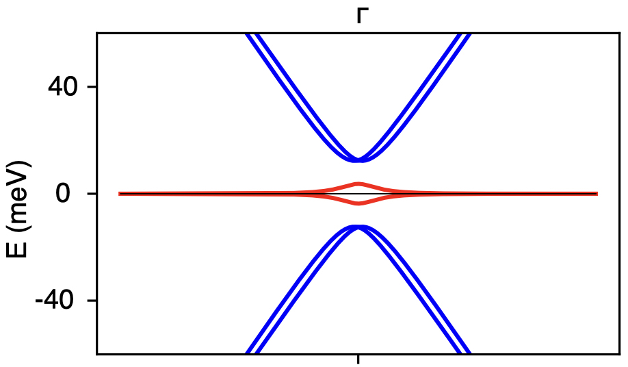
Figure 6: Many-body mean-field band-structure for a half filled flat band. Parameters used: chemical potential $\mu=0\,meV$, $\lambda=0\,meV$, $U=35\,meV$, with $\Gamma_{0}=U/4$, and $\gamma=12.6\,meV$. In this early preprint, full self-consistency has not been treated and will shortly be included in an updated version of the article.

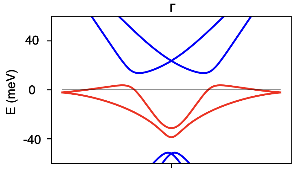
Figure 7: Many-body mean-field band-structure for $\nu_{E}=\mu/U>0$. Parameters used: chemical potential $\mu=35\,meV$, $\lambda=45\,meV$, $U=35\,meV$, with $\Gamma_{0}=U/4$, and $\gamma=32.9\,meV$. In this early preprint, full self-consistency has not been treated and will shortly be included in an updated version of the article.

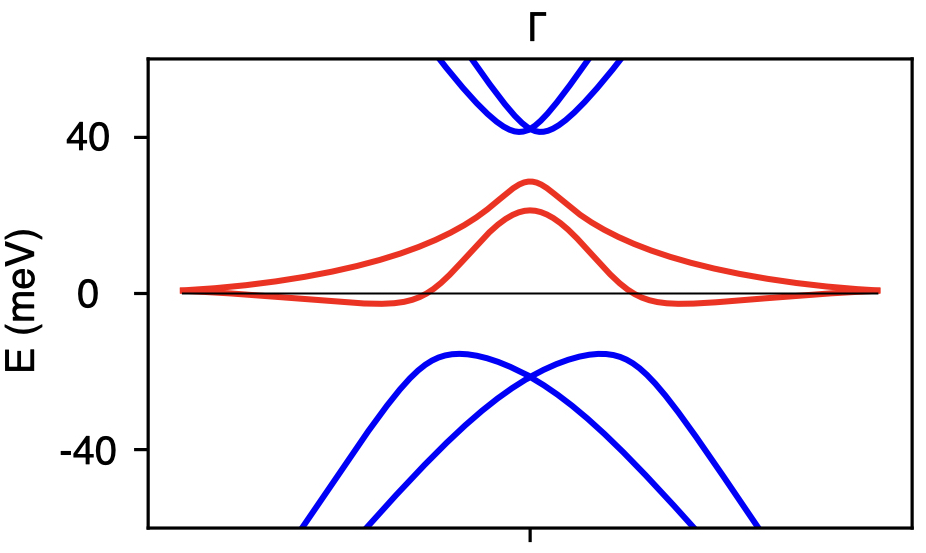
Figure 8: Many-body mean-field band-structure for $\nu_{E}=\mu/U<0$. Parameters used: chemical potential $\mu=-25\,meV$, $\lambda=-31\,meV$, $U=35\,meV$, with $\Gamma_{0}=U/4$, and $\gamma=29.0\,meV$. In this early preprint, full self-consistency has not been treated and will shortly be included in an updated version of the article.

VII Discussion

In this paper, we have conducted an initial examination of the physical consequences of including interactions into the SB heavy fermion description of MATBG. By taking an impurity limit of the SB model we have been able to identify the key scales in the problem, identifying the qualitative nature of the phase diagram. One of the robust consequences of the topological heavy fermion description is the presence of a conduction sea with a linear density of states at high energies. This effect means that the high doping states will typically be less strongly interacting, and more prone to the development of conventional Fermi liquid behavior.

There is, in our opinion, much that can be done to experimentally test the foundation of the SB description. In conventional heavy fermion systems, the presence of local moment behavior is immediately evident from the Curie-Weiss behavior of the magnetic susceptibility

$$\chi(T)\propto\frac{1}{T+\theta}$$ (65)

To what extent can such Curie Weiss behavior be detected from a Maxwell-analysis of existing field dependent compressibility measurements? It would be interesting to use existing field-dependent compressibility measurements to back-out the spin/valley susceptibility and directly measure the size of the moment. It would also be interesting to examine whether the upper and lower Hubbard bands observed in STM measurements, have a width that grows approximately linearly with the doping, which would provide direct evidence of the underlying topological conduction band.

Our qualitative analysis has found that the hybridization strength $\gamma_{0}\sim 25$meV obtained in the SB model, is likely too large to account for the observation of local moment behavior at filling factors of $|\nu|=3$, for which a considerably smaller value $\gamma_{0}^{*}\sim 6$meV is required. Can this be accounted for by polaronic effects? This is clearly a fruitful area for future exploration.

There is much that can be done to improve our approximate theoretical treatment of mixed valent MATBG. We have argued the importance of finding a treatment of this model that can handle the effects of valence fluctuations, and have proposed a vector auxiliary boson approach that appears to capture the essence of the valence fluctuations. There are many other theoretical methods that could be applied to MATBG, such as slave rotor approaches. and dynamical mean-field theory.

We end with a brief reflection on the nature of superconductivity in MATBG. Recent quasiparticle interference experiments have uncovered evidence of a possible d-wave nodal gap structure in the superconducting state. In a conventional superconductor this would be a sign of spin-singlet pairing. In MATBG, the presence of a valley-spin degeneracy with an $N_{f}=4$ fold degeneracy and the presence of strong local Hund’s interactions, raises the interesting possibility of spin or valley triplet paired states. An extension of the current model that includes the Hund’s interactions within the multi-electron Wannier states is thus highly desirable.

Acknowledgements

This work was supported by Office of Basic Energy Sciences, Material Sciences and Engineering Division, U.S. Department of Energy (DOE) under contract DE-FG02-99ER45790 (LLHL and PC).

Appendix A Derivation of the Flat Band Dirac Velocity in the Song-Bernevig Model

We derive an approximate expression for the Dirac velocity $v_{D}$ at the $K_{M}$ points of the Song and Bernevig model

$$H_{0}=\sum_{\begin{subarray}{c}{\textbf{k}}^{\prime}\in\text{MBZ}\\ {\textbf{G}}\end{subarray}}\Big{[}\sum_{aa^{\prime}\eta\sigma}\mathcal{H}_{a,a^{\prime}}^{\left(\eta\right)}\left({\textbf{k}}^{\prime}-{\textbf{G}}\right)c^{\dagger}_{{\textbf{k}}-{\textbf{G}},a\eta\sigma}c_{{\textbf{k}}^{\prime}-{\textbf{G}},a^{\prime}\eta\sigma}+\frac{\gamma_{0}}{\sqrt{N_{s}}}\sum_{\alpha a\eta\sigma}\big{(}[\phi^{\left(\eta\right)}\left({\textbf{k}}^{\prime}-{\textbf{G}},\gamma_{0}\right)]_{\alpha a}f^{\dagger}_{{\textbf{k}}^{\prime}\alpha\eta\sigma}c_{{\textbf{k}}^{\prime}-{\textbf{G}},a\eta\sigma}+\text{H.c.}\big{)}\Big{]}.$$ (66)

where the conduction electrons can take momenta outside the moiré Brillouin-zone and G are reciprocal lattice vectors. Here

$$\scalebox{0.95}{$\mathcal{H}^{\left(\eta\right)}\left(\textbf{k}\right)=\begin{pmatrix}&v_{\star}\left(\eta k_{x}\alpha_{0}+ik_{y}\alpha_{z}\right)\\ v_{\star}\left(\eta k_{x}\alpha_{0}-ik_{y}\alpha_{z}\right)&M\alpha_{x}\end{pmatrix}$}.$$ (67)

The matrix form factor is

$$\phi^{(\eta)}({\textbf{k}})\equiv\phi^{\left(\eta\right)}\left(\textbf{k},\gamma_{0}\right)=e^{\frac{-k^{2}\xi^{2}}{2}}\begin{pmatrix}\alpha_{0}+a_{\star}\left(\eta k_{x}\alpha_{x}+k_{y}\alpha_{y}\right),&0_{2\times 2}\end{pmatrix},$$ (68)

where $\gamma_{0}$ and $a_{\star}$ set the magnitude and length scale of the hybridization and $\xi$ is a damping factor proportional to the real space spread of the localized f-Wannier states. We also define the bandwidth $D=v_{\star}K_{\theta}$, $\tilde{\xi}=\xi K_{\theta}$ which will be useful later.

We focus on the physics at the $K_{M}$ or $K^{\prime}_{M}$ points and since $\phi_{\alpha a}^{\left(\eta\right)}\left({\textbf{k}}\right)$ decays exponentially, we keep only the three MBZs surrounding the moiré $K$ point, preserving the $C_{3z}$ symmetry about that point (Fig. 9).

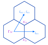
Figure 9: Sketch of the three moiré Brillouin zones around the $K_{M}$ point and the reciprocal lattice vectors.

Letting the eigenstates of the reduced model near the $K_{M}$ point to be

$$|\Psi(\delta{\textbf{k}})\rangle=\left(\sum_{\alpha}\psi_{\alpha}^{\left(f\right)}(\delta{\textbf{k}})f^{\dagger}_{{\textbf{k}}\alpha,\eta\sigma}+\sum_{a}\big{\{}\psi_{a}^{\left(0c\right)}(\delta{\textbf{k}})c^{\dagger}_{{\textbf{k}}a,\eta\sigma}+\psi_{a}^{\left(1c\right)}(\delta{\textbf{k}})c^{\dagger}_{{\textbf{k}}-{\textbf{G}}_{1},a,\eta\sigma}+\psi_{a}^{\left(2c\right)}(\delta{\textbf{k}})c^{\dagger}_{{\textbf{k}}-{\textbf{G}}_{2},a,\eta\sigma}\big{\}}\right)\biggr{\rvert}_{{\textbf{k}}=\textbf{K}_{M}+\delta{\textbf{k}}}|0\rangle$$

we can rewrite the Schrödinger equation $\hat{H}_{0}|\Psi(\delta{\textbf{k}})\rangle=E(\delta{\textbf{k}})|\Psi(\delta{\textbf{k}})\rangle$ in the first-quantized formalism as

$$H^{(\eta)}\left(\delta{\textbf{k}}\right)\Psi\left(\delta{\textbf{k}}\right)=E(\delta{\textbf{k}})\Psi\left(\delta{\textbf{k}}\right),$$ (69)

with the Hamiltonian matrix

$$\footnotesize H_{0}^{(\eta)}\left({\textbf{K}}_{M}+\delta{\textbf{k}}\right)=\begin{pmatrix}0&\phi^{(\eta)}({\textbf{K}}_{M}+\delta{\textbf{k}})&\phi^{(\eta)}({\textbf{K}}_{M}-\textbf{b}_{M2}+\textbf{b}_{M1}+\delta{\textbf{k}})&\phi^{(\eta)}({\textbf{K}}_{M}-\textbf{b}_{M2}+\delta{\textbf{k}})\\ \phi^{\dagger(\eta)}({\textbf{K}}_{M}+\delta{\textbf{k}})&\mathcal{H}^{(\eta)}\left({\textbf{K}}_{M}+\delta{\textbf{k}}\right)&0&0\\ \phi^{\dagger(\eta)}({\textbf{K}}_{M}-\textbf{b}_{M2}+\textbf{b}_{M1}+\delta{\textbf{k}})&0&\mathcal{H}^{(\eta)}({\textbf{K}}_{M}-\textbf{b}_{M2}+\textbf{b}_{M1}+\delta{\textbf{k}})&0\\ \phi^{\dagger(\eta)}({\textbf{K}}_{M}-\textbf{b}_{M2}+\delta{\textbf{k}})&0&0&\mathcal{H}^{(\eta)}({\textbf{K}}_{M}-\textbf{b}_{M2}+\delta{\textbf{k}})\end{pmatrix}$$ (70)

acting on the fourteen-dimensional spinor

$$\Psi\left(\delta{\textbf{k}}\right)=\left(\psi^{(f)}\left(\delta{\textbf{k}}\right),\psi^{(0c)}\left(\delta{\textbf{k}}\right),\psi^{(1c)}\left(\delta{\textbf{k}}\right),\psi^{(2c)}\left(\delta{\textbf{k}}\right)\right).$$ (71)

Defining ${\textbf{G}}_{0}=\textbf{0}$, ${\textbf{G}}_{1}=\textbf{b}_{M2}-\textbf{b}_{M1}$ and ${\textbf{G}}_{2}=\textbf{b}_{M2}$, the component form of the first-quantized formalism is

$$\sum_{i=0,1,2}\phi^{(\eta)}\left({\textbf{K}}_{M}-{\textbf{G}}_{i}+\delta{\textbf{k}}\right)\psi^{(ic)}=E\psi^{(f)}$$ (72)

$$\phi^{\dagger(\eta)}\left({\textbf{K}}_{M}-{\textbf{G}}_{i}+\delta{\textbf{k}}\right)\psi^{(f)}+\mathcal{H}^{(\eta)}\left({\textbf{K}}_{M}-{\textbf{G}}_{i}+\delta{\textbf{k}}\right)\psi^{(ic)}=E\psi^{(ic)},\;i=0,1,2.$$ (73)

Rearranging the second equation, we get $\psi^{(ic)}=\left(E-\mathcal{H}^{(\eta)}\left({\textbf{K}}_{M}-{\textbf{G}}_{i}+\delta{\textbf{k}}\right)\right)^{-1}\phi^{\dagger(\eta)}\left({\textbf{K}}_{M}-{\textbf{G}}_{i}+\delta{\textbf{k}}\right)\psi^{(f)}$ and inserting the expression into the first equation:

$$E\psi^{(f)}=\sum_{i=0,1,2}\phi^{(\eta)}\left({\textbf{K}}_{M}-{\textbf{G}}_{i}+\delta{\textbf{k}}\right)\left(E-\mathcal{H}^{(\eta)}\left({\textbf{K}}_{M}-{\textbf{G}}_{i}+\delta{\textbf{k}}\right)\right)^{-1}\phi^{\dagger(\eta)}\left({\textbf{K}}_{M}-{\textbf{G}}_{i}+\delta{\textbf{k}}\right)\psi^{(f)}.$$ (74)

The determinant of $\left(E-\mathcal{H}^{(\eta)}\left({\textbf{k}}\right)\right)$ is

$$E^{4}-E^{2}(M^{2}+2v_{\star}^{2}k^{2})+v_{\star}^{4}k^{4}$$ (75)

We neglect $\mathcal{O}\left(E^{2}\right)$ at $K_{M}$ and $K^{\prime}_{M}$ and using the identity $\eta^{2}=+1$,

$$\left(E-\mathcal{H}^{(\eta)}\left({\textbf{k}}\right)\right)^{-1}\approx$$

$$\frac{1}{v_{\star}^{4}|{\textbf{k}}|^{4}}\begin{pmatrix}(-M^{2}-v_{\star}^{2}|{\textbf{k}}|^{2})E\sigma_{0}-Mv_{\star}^{2}((k_{y}^{2}-k_{x}^{2})\sigma_{x}+2k_{x}k_{y}\eta\sigma_{y})&-v_{\star}^{3}|{\textbf{k}}|^{2}(\eta k_{x}\sigma_{0}+ik_{y}\sigma_{z})+Mv_{\star}E(\eta k_{x}\sigma_{x}-k_{y}\sigma_{y})\\ -v_{\star}^{3}|{\textbf{k}}|^{2}(\eta k_{x}\sigma_{0}-ik_{y}\sigma_{z})+Mv_{\star}E(\eta k_{x}\sigma_{x}-k_{y}\sigma_{y})&-v_{\star}^{2}|{\textbf{k}}|^{2}E\sigma_{0}\end{pmatrix}.$$ (76)

Using Eq. 76 in Eq. 74 and expand to first order in $\delta{\textbf{k}}$, where we also neglect the product of $\delta{\textbf{k}}$ and $E$, Eq. 74 reduces to

$$E\psi^{(f)} = -\frac{3\gamma_{K}^{2}\left(M^{2}+D^{2}\right)\left(K_{\theta}^{2}a_{\star}^{2}+1\right)}{D^{4}}E\psi^{(f)}-\frac{3M\gamma_{K}^{2}\left(2\left(1+a_{\star}^{2}K_{\theta}^{2}\right)+\tilde{\xi}^{2}\left(1-K_{\theta}a_{\star}\right)\left(K_{\theta}a_{\star}+1\right)\right)}{K_{\theta}D^{2}}\left(\sigma_{x}\delta k_{y}-\sigma_{y}\delta k_{x}\right)\psi^{(f)}$$ (77)

$$\approx - \left(\frac{3\gamma_{K}^{2}\left(K_{\theta}^{2}a_{\star}^{2}+1\right)}{D^{2}}E+\left(\frac{3M}{D}\right)\left(\frac{\gamma_{K}}{D}\right)^{2}\left(2\left(1+a_{\star}^{2}K_{\theta}^{2}\right)+\tilde{\xi}^{2}\left(1-K_{\theta}a_{\star}\right)\left(K_{\theta}a_{\star}+1\right)\right)v_{\star}\left(\sigma_{x}\delta k_{y}-\sigma_{y}\delta k_{x}\right)\right)\psi^{(f)}$$ (78)

where the last line is obtained because $D\gg M$ and $\gamma_{K}=\gamma_{0}e^{-\tilde{\xi}^{2}/2}$. We can identify a velocity $\tilde{v}_{D}$ and the Z factor from a self-energy treatment of the f-electrons, where the Dirac velocity at the $K_{M}$ points is

$$v_{D}=Z\tilde{v}_{D}.$$ (79)

The velocity

$$\tilde{v}_{D}=3\left(\frac{M}{D}\right)\left(\frac{\gamma_{K}}{D}\right)^{2}\left(2(1+a_{\star}^{2}K_{\theta}^{2})+\tilde{\xi}^{2}(1-K_{\theta}a_{\star})(K_{\theta}a_{\star}+1)\right)v_{\star},$$ (80)

and the Z factor is

$$Z=\left(1+3\left(\frac{\gamma_{K}}{D}\right)^{2}\left(K_{\theta}^{2}a_{\star}^{2}+1\right)\right)^{-1}\approx 1$$ (81)

because $(\gamma_{K}/D)\ll 1$. Rearranging yields the final result

$$E\psi^{(f)}=-v_{D}\,\left(\sigma_{x}\delta k_{y}-\sigma_{y}\delta k_{x}\right)\psi^{(f)},$$ (82)

linearized near the $K_{M}$ point. The Dirac velocity of the flat bands at the $K_{M}$ points is

$$v_{D}=3\left(\frac{M}{D}\right)\left(\frac{\gamma_{K}}{D}\right)^{2}\left(2(1+a_{\star}^{2}K_{\theta}^{2})+\tilde{\xi}^{2}(K_{\theta}a_{\star}+1)(1-K_{\theta}a_{\star})\right)v_{\star}.$$ (83)

Taking the $a_{\star}=0$ limit gives

$$v_{D}|_{a_{\star}=0}=3\left(\frac{M}{D}\right)\left(\frac{\gamma_{K}}{D}\right)^{2}\left(2+\tilde{\xi}^{2}\right)v_{\star}$$ (84)

Repeating the calculation for the $K^{\prime}_{M}$ point in the $\eta=+1$ valley results in $v_{D}\,\left(\sigma_{x}\delta k_{y}-\sigma_{y}\delta k_{x}\right)\psi^{(f)}=E\psi^{(f)}$, which has the same chirality as the Dirac cone at $K_{M}$ in the same valley. The Dirac cone structure of the topological heavy fermion model for the $K_{M}$ and $K^{\prime}_{M}$ points in the $\eta=-1$ valley is $-v_{D}\,\left(\sigma_{x}\delta k_{y}+\sigma_{y}\delta k_{x}\right)$ and $v_{D}\,\left(\sigma_{x}\delta k_{y}+\sigma_{y}\delta k_{x}\right)$. Note that the chirality of the Dirac cones in the $\eta=-1$ valley is opposite to the Dirac cones in the $\eta=+1$ valley.

References

- Li et al. [2010] G. Li, A. Luican, J. M. B. L. d. Santos, A. H. C. Neto, A. Reina, J. Kong, and E. Y. Andrei, Observation of Van Hove singularities in twisted graphene layers, Nature Physics 6, 109 (2010).
- Bistritzer and MacDonald [2011] R. Bistritzer and A. H. MacDonald, Moiré bands in twisted double-layer graphene, Proceedings of the National Academy of Sciences 108, 12233 (2011), publisher: Proceedings of the National Academy of Sciences.
- Cao et al. [2018a] Y. Cao, V. Fatemi, A. Demir, S. Fang, S. L. Tomarken, J. Y. Luo, J. D. Sanchez-Yamagishi, K. Watanabe, T. Taniguchi, E. Kaxiras, R. C. Ashoori, and P. Jarillo-Herrero, Correlated insulator behaviour at half-filling in magic-angle graphene superlattices, Nature 556, 80 (2018a), number: 7699 Publisher: Nature Publishing Group.
- Cao et al. [2018b] Y. Cao, V. Fatemi, S. Fang, K. Watanabe, T. Taniguchi, E. Kaxiras, and P. Jarillo-Herrero, Unconventional superconductivity in magic-angle graphene superlattices, Nature 556, 43 (2018b), number: 7699 Publisher: Nature Publishing Group.
- Andrei and MacDonald [2020] E. Y. Andrei and A. H. MacDonald, Graphene bilayers with a twist, Nature Materials 19, 1265 (2020), number: 12 Publisher: Nature Publishing Group.
- Andrei et al. [2021] E. Y. Andrei, D. K. Efetov, P. Jarillo-Herrero, A. H. MacDonald, K. F. Mak, T. Senthil, E. Tutuc, A. Yazdani, and A. F. Young, The marvels of moiré materials, Nature Reviews Materials 6, 201 (2021), number: 3 Publisher: Nature Publishing Group.
- Lian et al. [2021] B. Lian, Z.-D. Song, N. Regnault, D. K. Efetov, A. Yazdani, and B. A. Bernevig, Twisted bilayer graphene. IV. Exact insulator ground states and phase diagram, Physical Review B 103, 205414 (2021), publisher: American Physical Society.
- Liu et al. [2019] J. Liu, Z. Ma, J. Gao, and X. Dai, Quantum Valley Hall Effect, Orbital Magnetism, and Anomalous Hall Effect in Twisted Multilayer Graphene Systems, Physical Review X 9, 031021 (2019), publisher: American Physical Society.
- Repellin et al. [2020] C. Repellin, Z. Dong, Y.-H. Zhang, and T. Senthil, Ferromagnetism in Narrow Bands of Moir\’e Superlattices, Physical Review Letters 124, 187601 (2020), publisher: American Physical Society.
- Wu and Das Sarma [2020] F. Wu and S. Das Sarma, Collective Excitations of Quantum Anomalous Hall Ferromagnets in Twisted Bilayer Graphene, Physical Review Letters 124, 046403 (2020), publisher: American Physical Society.
- Pixley and Andrei [2019] J. H. Pixley and E. Y. Andrei, Ferromagnetism in magic-angle graphene, Science 365, 543 (2019), publisher: American Association for the Advancement of Science.
- Cao et al. [2020] Y. Cao, D. Chowdhury, D. Rodan-Legrain, O. Rubies-Bigorda, K. Watanabe, T. Taniguchi, T. Senthil, and P. Jarillo-Herrero, Strange Metal in Magic-Angle Graphene with near Planckian Dissipation, Physical Review Letters 124, 076801 (2020), number: 7.
- Lyu et al. [2021] R. Lyu, Z. Tuchfeld, N. Verma, H. Tian, K. Watanabe, T. Taniguchi, C. N. Lau, M. Randeria, and M. Bockrath, Strange metal behavior of the Hall angle in twisted bilayer graphene, Physical Review B 103, 245424 (2021), number: 24.
- Das Sarma and Wu [2022] S. Das Sarma and F. Wu, Strange metallicity of moiré twisted bilayer graphene, Physical Review Research 4, 033061 (2022), number: 3.
- Cha et al. [2021] P. Cha, A. A. Patel, and E.-A. Kim, Strange Metals from Melting Correlated Insulators in Twisted Bilayer Graphene, Physical Review Letters 127, 266601 (2021), publisher: American Physical Society.
- Ghawri et al. [2022] B. Ghawri, P. S. Mahapatra, M. Garg, S. Mandal, S. Bhowmik, A. Jayaraman, R. Soni, K. Watanabe, T. Taniguchi, H. R. Krishnamurthy, M. Jain, S. Banerjee, U. Chandni, and A. Ghosh, Breakdown of semiclassical description of thermoelectricity in near-magic angle twisted bilayer graphene, Nature Communications 13, 1522 (2022), number: 1 Publisher: Nature Publishing Group.
- Arora et al. [2020] H. S. Arora, R. Polski, Y. Zhang, A. Thomson, Y. Choi, H. Kim, Z. Lin, I. Z. Wilson, X. Xu, J.-H. Chu, K. Watanabe, T. Taniguchi, J. Alicea, and S. Nadj-Perge, Superconductivity in metallic twisted bilayer graphene stabilized by WSe2, Nature 583, 379 (2020), number: 7816 Publisher: Nature Publishing Group.
- Polshyn et al. [2019] H. Polshyn, M. Yankowitz, S. Chen, Y. Zhang, K. Watanabe, T. Taniguchi, C. R. Dean, and A. F. Young, Large linear-in-temperature resistivity in twisted bilayer graphene, Nature Physics 15, 1011 (2019), number: 10 Publisher: Nature Publishing Group.
- Jaoui et al. [2022] A. Jaoui, I. Das, G. Di Battista, J. Díez-Mérida, X. Lu, K. Watanabe, T. Taniguchi, H. Ishizuka, L. Levitov, and D. K. Efetov, Quantum critical behaviour in magic-angle twisted bilayer graphene, Nature Physics 18, 633 (2022), number: 6.
- Codecido et al. [2019] E. Codecido, Q. Wang, R. Koester, S. Che, H. Tian, R. Lv, S. Tran, K. Watanabe, T. Taniguchi, F. Zhang, M. Bockrath, and C. N. Lau, Correlated insulating and superconducting states in twisted bilayer graphene below the magic angle, Science Advances 5, eaaw9770 (2019), number: 9.
- Yankowitz et al. [2019] M. Yankowitz, S. Chen, H. Polshyn, Y. Zhang, K. Watanabe, T. Taniguchi, D. Graf, A. F. Young, and C. R. Dean, Tuning superconductivity in twisted bilayer graphene, Science 363, 1059 (2019), publisher: American Association for the Advancement of Science.
- Bultinck et al. [2020] N. Bultinck, E. Khalaf, S. Liu, S. Chatterjee, A. Vishwanath, and M. P. Zaletel, Ground State and Hidden Symmetry of Magic-Angle Graphene at Even Integer Filling, Physical Review X 10, 031034 (2020), publisher: American Physical Society.
- Xie and MacDonald [2020] M. Xie and A. MacDonald, Nature of the Correlated Insulator States in Twisted Bilayer Graphene, Physical Review Letters 124, 097601 (2020), publisher: American Physical Society.
- Zhang et al. [2020] Y. Zhang, K. Jiang, Z. Wang, and F. Zhang, Correlated insulating phases of twisted bilayer graphene at commensurate filling fractions: A Hartree-Fock study, Physical Review B 102, 035136 (2020), publisher: American Physical Society.
- Balents et al. [2020] L. Balents, C. R. Dean, D. K. Efetov, and A. F. Young, Superconductivity and strong correlations in moiré flat bands, Nature Physics 16, 725 (2020).
- Lian et al. [2019] B. Lian, Z. Wang, and B. A. Bernevig, Twisted Bilayer Graphene: A Phonon-Driven Superconductor, Physical Review Letters 122, 257002 (2019), publisher: American Physical Society.
- Liu et al. [2021] S. Liu, E. Khalaf, J. Y. Lee, and A. Vishwanath, Nematic topological semimetal and insulator in magic-angle bilayer graphene at charge neutrality, Physical Review Research 3, 013033 (2021), publisher: American Physical Society.
- Liu et al. [2018] C.-C. Liu, L.-D. Zhang, W.-Q. Chen, and F. Yang, Chiral Spin Density Wave and $d+id$ Superconductivity in the Magic-Angle-Twisted Bilayer Graphene, Physical Review Letters 121, 217001 (2018), publisher: American Physical Society.
- Wu et al. [2018] F. Wu, A. MacDonald, and I. Martin, Theory of Phonon-Mediated Superconductivity in Twisted Bilayer Graphene, Physical Review Letters 121, 257001 (2018), publisher: American Physical Society.
- Xie et al. [2020] F. Xie, Z. Song, B. Lian, and B. A. Bernevig, Topology-Bounded Superfluid Weight in Twisted Bilayer Graphene, Physical Review Letters 124, 167002 (2020), publisher: American Physical Society.
- Xu and Balents [2018] C. Xu and L. Balents, Topological Superconductivity in Twisted Multilayer Graphene, Physical Review Letters 121, 087001 (2018), publisher: American Physical Society.
- Lewandowski et al. [2021] C. Lewandowski, D. Chowdhury, and J. Ruhman, Pairing in magic-angle twisted bilayer graphene: Role of phonon and plasmon umklapp, Physical Review B 103, 235401 (2021), publisher: American Physical Society.
- Khalaf et al. [2021] E. Khalaf, S. Chatterjee, N. Bultinck, M. P. Zaletel, and A. Vishwanath, Charged skyrmions and topological origin of superconductivity in magic-angle graphene, Science Advances 7, eabf5299 (2021), publisher: American Association for the Advancement of Science.
- König et al. [2020] E. J. König, P. Coleman, and A. M. Tsvelik, Spin magnetometry as a probe of stripe superconductivity in twisted bilayer graphene, Physical Review B 102, 104514 (2020), publisher: American Physical Society.
- Chichinadze et al. [2020] D. V. Chichinadze, L. Classen, and A. V. Chubukov, Nematic superconductivity in twisted bilayer graphene, Physical Review B 101, 224513 (2020), publisher: American Physical Society.
- González and Stauber [2019] J. González and T. Stauber, Kohn-Luttinger Superconductivity in Twisted Bilayer Graphene, Physical Review Letters 122, 026801 (2019), publisher: American Physical Society.
- Guinea and Walet [2018] F. Guinea and N. R. Walet, Electrostatic effects, band distortions, and superconductivity in twisted graphene bilayers, Proceedings of the National Academy of Sciences 115, 13174 (2018), publisher: Proceedings of the National Academy of Sciences.
- Huang et al. [2019] T. Huang, L. Zhang, and T. Ma, Antiferromagnetically ordered Mott insulator and d+id superconductivity in twisted bilayer graphene: a quantum Monte Carlo study, Science Bulletin 64, 310 (2019).
- Isobe et al. [2018] H. Isobe, N. F. Yuan, and L. Fu, Unconventional Superconductivity and Density Waves in Twisted Bilayer Graphene, Physical Review X 8, 041041 (2018), publisher: American Physical Society.
- Julku et al. [2020] A. Julku, T. J. Peltonen, L. Liang, T. T. Heikkilä, and P. Törmä, Superfluid weight and Berezinskii-Kosterlitz-Thouless transition temperature of twisted bilayer graphene, Physical Review B 101, 060505 (2020), publisher: American Physical Society.
- Kennes et al. [2018] D. M. Kennes, J. Lischner, and C. Karrasch, Strong correlations and $d+\mathit{id}$ superconductivity in twisted bilayer graphene, Physical Review B 98, 241407 (2018), publisher: American Physical Society.
- Wong et al. [2020] D. Wong, K. P. Nuckolls, M. Oh, B. Lian, Y. Xie, S. Jeon, K. Watanabe, T. Taniguchi, B. A. Bernevig, and A. Yazdani, Cascade of electronic transitions in magic-angle twisted bilayer graphene, Nature 582, 198 (2020), number: 7811 Publisher: Nature Publishing Group.
- Saito et al. [2021a] Y. Saito, F. Yang, J. Ge, X. Liu, T. Taniguchi, K. Watanabe, J. I. A. Li, E. Berg, and A. F. Young, Isospin Pomeranchuk effect in twisted bilayer graphene, Nature 592, 220 (2021a), number: 7853 Publisher: Nature Publishing Group.
- Lu et al. [2019] X. Lu, P. Stepanov, W. Yang, M. Xie, M. A. Aamir, I. Das, C. Urgell, K. Watanabe, T. Taniguchi, G. Zhang, A. Bachtold, A. H. MacDonald, and D. K. Efetov, Superconductors, orbital magnets and correlated states in magic-angle bilayer graphene, Nature 574, 653 (2019), number: 7780 Publisher: Nature Publishing Group.
- Rozen et al. [2021] A. Rozen, J. M. Park, U. Zondiner, Y. Cao, D. Rodan-Legrain, T. Taniguchi, K. Watanabe, Y. Oreg, A. Stern, E. Berg, P. Jarillo-Herrero, and S. Ilani, Entropic evidence for a Pomeranchuk effect in magic-angle graphene, Nature 592, 214 (2021), number: 7853 Publisher: Nature Publishing Group.
- Xie et al. [2019] Y. Xie, B. Lian, B. Jäck, X. Liu, C.-L. Chiu, K. Watanabe, T. Taniguchi, B. A. Bernevig, and A. Yazdani, Spectroscopic signatures of many-body correlations in magic-angle twisted bilayer graphene, Nature 572, 101 (2019).
- Song et al. [2019] Z. Song, Z. Wang, W. Shi, G. Li, C. Fang, and B. A. Bernevig, All Magic Angles in Twisted Bilayer Graphene are Topological, Physical Review Letters 123, 36401 (2019), publisher: American Physical Society.
- Zou et al. [2018] L. Zou, H. C. Po, A. Vishwanath, and T. Senthil, Band structure of twisted bilayer graphene: Emergent symmetries, commensurate approximants, and Wannier obstructions, Physical Review B 98, 085435 (2018), publisher: American Physical Society.
- Efimkin and MacDonald [2018] D. K. Efimkin and A. H. MacDonald, Helical network model for twisted bilayer graphene, Physical Review B 98, 035404 (2018), publisher: American Physical Society.
- Nuckolls et al. [2020] K. P. Nuckolls, M. Oh, D. Wong, B. Lian, K. Watanabe, T. Taniguchi, B. A. Bernevig, and A. Yazdani, Strongly correlated Chern insulators in magic-angle twisted bilayer graphene, Nature 588, 610 (2020), number: 7839 Publisher: Nature Publishing Group.
- Hejazi et al. [2021] K. Hejazi, X. Chen, and L. Balents, Hybrid Wannier Chern bands in magic angle twisted bilayer graphene and the quantized anomalous Hall effect, Physical Review Research 3, 013242 (2021), publisher: American Physical Society.
- Saito et al. [2021b] Y. Saito, J. Ge, L. Rademaker, K. Watanabe, T. Taniguchi, D. A. Abanin, and A. F. Young, Hofstadter subband ferromagnetism and symmetry-broken Chern insulators in twisted bilayer graphene, Nature Physics 17, 478 (2021b), number: 4 Publisher: Nature Publishing Group.
- Choi et al. [2021] Y. Choi, H. Kim, Y. Peng, A. Thomson, C. Lewandowski, R. Polski, Y. Zhang, H. S. Arora, K. Watanabe, T. Taniguchi, J. Alicea, and S. Nadj-Perge, Correlation-driven topological phases in magic-angle twisted bilayer graphene, Nature 589, 536 (2021), number: 7843 Publisher: Nature Publishing Group.
- Wu et al. [2021] S. Wu, Z. Zhang, K. Watanabe, T. Taniguchi, and E. Y. Andrei, Chern insulators, van Hove singularities and topological flat bands in magic-angle twisted bilayer graphene, Nature Materials 20, 488 (2021), number: 4 Publisher: Nature Publishing Group.
- Kang and Vafek [2020] J. Kang and O. Vafek, Non-Abelian Dirac node braiding and near-degeneracy of correlated phases at odd integer filling in magic-angle twisted bilayer graphene, Physical Review B 102, 035161 (2020), publisher: American Physical Society.
- Po et al. [2019] H. C. Po, L. Zou, T. Senthil, and A. Vishwanath, Faithful tight-binding models and fragile topology of magic-angle bilayer graphene, Physical Review B 99, 195455 (2019), publisher: American Physical Society.
- Lian et al. [2020] B. Lian, F. Xie, and B. A. Bernevig, Landau level of fragile topology, Physical Review B 102, 041402 (2020), publisher: American Physical Society.
- Song and Bernevig [2022] Z.-D. Song and B. A. Bernevig, Magic-Angle Twisted Bilayer Graphene as a Topological Heavy Fermion Problem, Phys. Rev. Lett. 129, 047601 (2022), publisher: American Physical Society.
- Shi and Dai [2022] H. Shi and X. Dai, Heavy fermion representation for twisted bilayer graphene systems, Physical Review B 106, 245129 (2022), arXiv:2209.09515 [cond-mat].
- Chou and Sarma [2022] Y.-Z. Chou and S. D. Sarma, Kondo lattice model in magic-angle twisted bilayer graphene (2022), arXiv:2211.15682 [cond-mat].
- Hu et al. [2023a] H. Hu, B. A. Bernevig, and A. M. Tsvelik, Kondo Lattice Model of Magic-Angle Twisted-Bilayer Graphene: Hund’s Rule, Local-Moment Fluctuations, and Low-Energy Effective Theory (2023a), arXiv:2301.04669 [cond-mat].
- Hu et al. [2023b] H. Hu, G. Rai, L. Crippa, J. Herzog-Arbeitman, D. Călugăru, T. Wehling, G. Sangiovanni, R. Valenti, A. M. Tsvelik, and B. A. Bernevig, Symmetric Kondo Lattice States in Doped Strained Twisted Bilayer Graphene (2023b), arXiv:2301.04673 [cond-mat].
- Zhou and Song [2023] G.-D. Zhou and Z.-D. Song, Kondo Phase in Twisted Bilayer Graphene – A Unified Theory for Distinct Experiments (2023), arXiv:2301.04661 [cond-mat].
- Hewson [1993] A. C. Hewson, \sl \sl The Kondo Problem to Heavy Fermions (Cambridge University Press, Cambridge, 1993).
- Kondo [1964] J. Kondo, Resistance Minimum in Dilute Magnetic Alloys, Progress of Theoretical Physics 32, 37 (1964).
- Kondo [1962] J. Kondo, Anomalous Hall Effect and Magnetoresistance of Ferromagnetic Metals, Progress of Theoretical Physics 27, 772 (1962).
- Coleman [2007] P. Coleman, Heavy Fermions: electrons at the edge of magnetism (2007), arXiv:cond-mat/0612006.
- Si and Steglich [2010] Q. Si and F. Steglich, Heavy Fermions and Quantum Phase Transitions, Science 329, 1161 (2010), publisher: American Association for the Advancement of Science.
- Wirth and Steglich [2016] S. Wirth and F. Steglich, Exploring heavy fermions from macroscopic to microscopic length scales, Nature Reviews Materials 1, 1 (2016), number: 10 Publisher: Nature Publishing Group.
- Stewart [1984] G. R. Stewart, Heavy-fermion systems, Reviews of Modern Physics 56, 755 (1984), publisher: American Physical Society.
- Dzero et al. [2010] M. Dzero, K. Sun, V. Galitski, and P. Coleman, Topological Kondo Insulators, Physical Review Letters 104, 106408 (2010), publisher: American Physical Society.
- Doniach [1977] S. Doniach, The Kondo lattice and weak antiferromagnetism, Physica B+C 91, 231 (1977).
- Jullien et al. [1977] R. Jullien, J. N. Fields, and S. Doniach, Zero-temperature real-space renormalization-group method for a Kondo-lattice model Hamiltonian, Physical Review B 16, 4889 (1977), publisher: American Physical Society.
- Ruderman and Kittel [1954] M. A. Ruderman and C. Kittel, Indirect Exchange Coupling of Nuclear Magnetic Moments by Conduction Electrons, Physical Review 96, 99 (1954), publisher: American Physical Society.
- Kasuya [1956] T. Kasuya, \sl \sl Indirect Exchange Coupling of Nuclear Magnetic Moments by Conduction Electrons, Prog. Theo. Phys. 16, 45 (1956).
- Yosida [1957] K. Yosida, \sl \sl Magnetic Properties of Cu-Mn Alloys, Phys. Rev. 106, 896 (1957).
- Schrieffer and Wolff [1966] J. R. Schrieffer and P. Wolff, \sl \sl Relation between the Anderson and Kondo Hamiltonians, Phys. Rev. 149, 491 (1966).
- Coqblin and Schrieffer [1969] B. Coqblin and J. R. Schrieffer, Exchange Interaction in Alloys with Cerium Impurities, Physical Review 185, 847 (1969), publisher: American Physical Society.
- Barnes [1976] S. E. Barnes, New method for the Anderson model, Journal of Physics F: Metal Physics 6, 1375 (1976).
- Coleman [1984] P. Coleman, \sl \sl New approach to the mixed-valence problem, Phys. Rev. B 29, 3035 (1984).