Learned Lossless Compression for JPEG via Frequency-Domain Prediction

Abstract

JPEG images can be further compressed to enhance the storage and transmission of large-scale image datasets. Existing learned lossless compressors for RGB images cannot be well transferred to JPEG images due to the distinguishing distribution of DCT coefficients and raw pixels. In this paper, we propose a novel framework for learned lossless compression of JPEG images that achieves end-to-end optimized prediction of the distribution of decoded DCT coefficients. To enable learning in the frequency domain, DCT coefficients are partitioned into groups to utilize implicit local redundancy. An autoencoder-like architecture is designed based on the weight-shared blocks to realize entropy modeling of grouped DCT coefficients and independently compress the priors. We attempt to realize learned lossless compression of JPEG images in the frequency domain. Experimental results demonstrate that the proposed framework achieves superior or comparable performance in comparison to most recent lossless compressors with handcrafted context modeling for JPEG images.

Figure 1: Illustration of our proposed recompression framework. To implement a frequency domain recompression, JPEG bitstream is incompletely decoded to DCT coefficients. These DCT coefficients are further compressed with arithmetic coding, which benefits from a carefully designed distribution predictor. Besides, this distribution predictor compress the priors about the distributions as side information that contained in the recompressed bitstream.

1 Introduction

Storage and transmission of large-scale image datasets, e.g., ImageNet [19] and Flicker [4], are necessary for training deep neural networks (DNNs). JPEG [47] is the most popular image compression standard. The JPEG codec leverages transform coding, chroma subsampling, quantization and entropy coding in a sequence to remove spatial redundancies. However, JPEG is inferior to JPEG2000[40] and BPG[12] due to fixed $8\times 8$ discrete cosine transform (DCT) and Huffman coding. Recently, task-specific (lossy) and task-free (lossless) methods have been developed to further compress JPEG images.

Task-specific methods compress the JPEG images with the guidance of image processing tasks. Liu et. al [31] developed DeepN-JPEG, a JPEG compression framework for image classification based on the high-frequency bias observed in experiments. DeepN-JPEG achieves about 350% compression ratio on ImageNet without degrading the classification performance of deep neural networks. Li et. al [30] optimized JPEG quantization table with sorted random search and composite heuristic optimization and achieves a gain of 20%-200% compression ratio at the same accuracy. Besides storage reduction, task-specific methods can also improve the performance of image processing. For example, Choi et. al [18] estimated image-specific quantization tables with deep neural networks to improve the tasks of image classification performance, image captioning, and visual quality. However, task-specific compression methods are lossy, as they introduce extra distortion to the input JPEG images by adjusting the quantization tables.

Task-free methods are developed for universal compression of JPEG images. Lepton [26] is one of the representative work that utilizes manufactured context models for precise distribution prediction on each discrete cosine transformation (DCT) coefficient. Lepton provides about 23% bitrate saving over original JPEG images and achieves efficient decompression via a parallelized arithmetic coding. Besides Lepton, mozjpeg [5] and Brunsli [2] can also reduce the size of JPEG images by around 10% and 22% without introducing extra distortion, respectively. It is worth mentioning that universal lossless compression algorithms such as Lempel-Ziv-Markov chain-Algorithm (LZMA) [38] can also be employed on the JPEG images, but can only achieve a trivial compression gain, e.g., about 1%. Although these lossless JPEG compressors are practical and efficient, they suffer from tedious design of context models. For example, Lepton uses kinds of manually designed contexts to model the conditional distribution and requires enormous statistical experiments to determine the parameters for prediction.

Recent development in end-to-end compression reveals the potential of getting rid of tedious handcrafted context modeling. The neural-network-based entropy models are developed for differentiable distribution modeling of the latent representations. However, existing methods for learned lossless compression are developed for RGB images and cannot be directly employed to effectively compress JPEG images (i.e., DCT coefficients). Recalling lossy image compression, the hyper-prior based entropy model [11] can dramatically improve the rate-distortion performance of end-to-end image compression methods. In the hyper-prior model, the latent representations is supposed to follow certain parameterized distributions (e.g. Gaussian distribution and Laplace distribution). Then the parameters for these distributions are predicted with a neural network, and utilized for arithmetic coding. To enhance the decoding process, the information about these distributions is compressed and transmitted to the decoder as a packed prior.

Inspired by the hyper-prior model, in this paper, we propose a novel framework for lossless compression of JPEG images. As depicted in Figure 1, the proposed framework achieves end-to-end optimized distribution prediction for arithmetic coding of DCT coefficients by incompletely decoding JPEG bitstream. The contributions of this paper are summarized as below.

• We propose a novel framework for learned lossless compression of JPEG images. The proposed framework achieves comparable performance to the carefully designed traditional methods such as Lepton.

• We achieve end-to-end optimized distribution prediction of DCT coefficients incompletely decoded from the JPEG images via frequency partitioning and learning. Grouped DCT coefficients are adopted to improve the compression performance.

• We design the weight-shared residual blocks to constitute an autoencoder-like architecture that improves compression performance and maintains a low memory consumption during training.

This work is the learned lossless compressor specifically designed for JPEG images. Different from existing learned lossless methods, the DCT coefficients are partitioned into several frequency groups to enable end-to-end optimized distrubtion prediction. An autoencoder-like architecture is designed based on weight-shared blocks to realize entropy modeling of grouped DCT coefficients and independently compress the priors. Experimental results show that the proposed method outperforms LZMA, mozjpeg, and Brunsli, and is comparable to Lepton in terms of compression ratio.

2 Related Work

2.1 Learned Lossless Compression

Lossless compression has been studied for both universal data and images for a long time, and recent development of deep learning methods has stimulated new researches in this field. For example, DeepZip [23] used recurrent neural networks (RNNs) and bits-back coding [28] to realize lossless compression for universal data, especially for sequence data. Aiming at lossless image compression, L3C [32] estimated the distribution of each pixel in RGB domain with a serialized hierarchical probabilistic model. Moreover, Mentzer et. al [34] and Cheng et. al [17] suggested that compressing residual of compressed image with traditional methods is also feasible for lossless image compression with end-to-end models.

However, these models are not practical for JPEG image recompression for their low efficiency. The JPEG images have been lossy compressed and typically have a file size more than 20x smaller than the original image. But the most efficient lossless compression methods can only achieve 2x to 3x compression rate. Thus, the lossless compression in RGB domain cannot improve the compression rate of JPEG images. Therefore, a DCT domain compression is required.

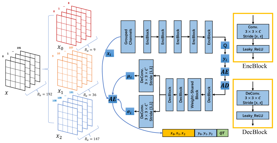
Figure 2: The left part is the data processing: $B_{\alpha}$ represents the number of channels. Then Frequency Band is spilt into three Grouped Channels. The right part is the network structure: The input is Grouped Channels, namely $x_{i}$. Conv and DeConv is the convolution layer with $3\times 3$ kernel, $C$ channels and $[s,s]$ stride. Besides, the stride of first two EncBlocks and the last two DecBlocks are $[2,2]$, the others are $[1,1]$. We set $C=48$ of the last EncBlock, and the others are $384$. Leaky_ReLU is the activation function. Q is the quantization, $y_{i}$ is the features to be encoded. AE and AD are the arithmetic encoder and arithmetic decoder. $\mu_{i}$, $\sigma_{i}$ are the parameters for arithmetic coder. $C_{i}$ is the output channel and it is the same with input channels of grouped channels. Then $x_{i}$, $y_{i}$ and QT are compressed to form the final bitstream.

2.2 Frequency Learning

Conventional neural networks utilize RGB images as input, where the spatial information would be captured. For saving decoding time of JPEG images, methods exploiting DCT coefficients are explored. Gueguen et. al [24] trained a convolutional neural network (CNN) directly on the DCT coefficient acquired from JPEG bitstream, which gains acceleration compared with standard residual network (ResNet). Ehrlich et. al [21] redefined convolution, batch normalization, and ReLU leveraging the linearity of the JPEG transform. Xu et. al [48] used DCT coefficients as input and selected the most significant components to perform image inference, which reduce the burden of data transmission. This method is verified in image detection and classification, with a superior performance over conventional methods. These methods proves the potential of frequency learning and inspire us to use end-to-end models for lossless frequency compression.

3 Methodology

This section demonstrates the framework for lossless compression of JPEG images. We first present the pipeline of the proposed framework, and then describe implementation details of the end-to-end distribution predictor.

3.1 Proposed Framework

The proposed framework is developed for the DCT coefficients obtained by incomplete decoding of JPEG images. For clarity, we denote the tensor of DCT coefficients as $x\in\mathbb{R}^{H\times W\times 192}$, that consists of 64 frequency components of DCT coefficients over 3 color planes. The details of the arrangement is described in Section 3.2. As shown in Figure 2, $x$ is partitioned into several frequency groups in the sense of “low frequency”, “middle frequency”, and “high frequency”. The partitioned groups are denoted as $x_{0},x_{1},\cdots,x_{n}$ with $x_{i}\in\mathbb{R}^{H\times W\times C_{i}}$ and $\sum_{i}C_{i}=192$. $x_{i}$ is supposed to obey a multivariate Gaussian distribution, where the mean $\mu_{i}$ and the scale $\sigma_{i}$ are predicted with distribution predictor. Moreover, the distributions of each group are estimated separately with a specific distribution predictor. The predictors share the same structure, while the parameters are learned independently since the scale and correlation of different frequency is distinguished. Overall, the predictors are constructed like an auto-encoder, where the output is the means and scales for Gaussian distribution. Here, the encoder and decoder are denoted as $\mathcal{E}_{i}$ and $\mathcal{D}_{i}$.

$$y_{i}=\lfloor\mathcal{E}_{i}(x_{i})\rceil,\quad[\mu_{i},\sigma_{i}]=\mathcal{D}_{i}(y_{i}),$$ (1)

where $\lfloor\cdot\rceil$ represents the rounding operation and $y_{i}$ is the quantized output of the encoder. $y_{i}$ is the prior of $\mu_{i}$ and $\sigma_{i}$, and is quantized to integer symbols for entropy coding. $y_{i}$ is encoded and embedded into the bitstream, and is transmitted to the decoder.

Considering end-to-end training for the distribution predictors, the whole framework is optimized based on a joint loss to balance the performance over all frequency components. The loss function is designed as

$$L =\sum_{i}(R_{x_{i}}+\lambda R_{y_{i}})$$

$$=\sum_{i}\left(\mathbb{E}[-\log_{2}(p_{x_{i}})]+\lambda\mathbb{E}[-\log_{2}(p_{y_{i}})]\right),$$ (2)

where $R_{x_{i}}$ and $R_{y_{i}}$ is the average bit consumption of $x_{i}$ and $y_{i}$. The probability of $x_{i}$ can be inferred from the parameterized Gaussian distritbution. With the estimated $\mu_{i}$ and $\sigma_{i}$, the probability of integer symbol $a=x_{i}^{h,w}$ in $x_{i}$ is

$$p(a,\sigma,\mu)=\int_{a-0.5}^{a+0.5}\frac{1}{\sqrt{2\pi}\sigma}e^{-\frac{(a-\mu)^{2}}{2\sigma^{2}}},$$ (3)

where $\mu=\mu_{i}^{h,w}$ and $\sigma=\sigma_{i}^{h,w}$ are the mean and scale on the corresponding positions of $\mu_{i}$ and $\sigma_{i}$. The probability of $y_{i}$ is estimated with the method introduced in [10]. It is worthy mentioning that $\lambda$ in Equation (3.1) is expected to be 1 for the lossless compression task, but we find that progressively increasing $\lambda$ would improve the compression performance. The details of the tuning strategy is elaborated in Section 5.2.

3.2 Implementation Details

Arrangement of DCT Coefficients . Suppose the original image has a size of $N\times M$, then these coefficients are stored in $\lceil\frac{N}{8}\rceil\times\lceil\frac{M}{8}\rceil$ blocks of $8\times 8$, where $\lceil\cdot\rceil$ means the ceil operation. Besides, considering the three color planes (i.e., Y, Cb, and Cr) adopted in JPEG for compressing color image, $x$ has the shape of $\lceil\frac{N}{8}\rceil\times\lceil\frac{M}{8}\rceil\times 8\times 8\times 3$. To simplify the notation of this 5-dimensional tensor, we rearrange the coefficients according to their frequency and color planes, while keep the first two dimensions unchanged. As shown in Figure 4, the $8\times 8$ DCT coefficients in each block is indexed in a Zig-Zag order ranging from 0 to 63. The coefficients on different color planes with the same index placed in the following order: Y$\rightarrow$Cb$\rightarrow$Cr$\rightarrow$Y$\rightarrow$Cb$\rightarrow$Cr$\cdots$. Moreover, we define $H\equiv\lceil\frac{N}{8}\rceil,W\equiv\lceil\frac{M}{8}\rceil$. Then the 5-dimensional tensor $x$ is reshaped into the shape mentioned before, as $H\times W\times 192$.

Network Architecture. The main body is the autoencoder as shown in Figure 2, including encoder and decoder. Encoder consists of five EncBlock, and each EncBlock is composed of convolutional layer with $3\times 3$ kernel and leaky ReLU activation function. The first two EncBlock have stride with $2$, thus encoder subsamples with $4$ times to transfer input coefficients $x_{i}$ into $\dot{y}_{i}$. Then we quantize $\dot{y}_{i}$ into $y_{i}$ for arithmetic encoding and decoding. And decoder has DecBlock and Weight-Shared Block, and each DecBlock is composed of deconvolutional layer with $3\times 3$ kernel and leaky ReLU activation function. The last two DecBlock has stride with $2$ and decoder upsamples the extracted feature with $4$ time. Then the last convolutional layers output the parameters of Gaussian $\mu_{i}$ and $\sigma_{i}$ to generate the probability of input $x_{i}$.

Weight-Shared Block. The weight-shared block in Figure 3 is introduced in the decoder side to facilitate training. When Figure 3($a$) has three iterations, Figure 3($a$) has the same structure with Figure 3($b$). But three blocks in Figure 3($a$) share the same parameters. Different from the ResNet in [25], the weight of these blocks share the same weights. Thus we name it weight-shared block. Besides, it has forward flow(from input to output) as shown in the left of Figure 3($a$) and the backward flow(from output to input) as shown in the right of Figure 3($a$) at the same time. It reduces the complexity of decoder, and improve the compression gain.

Figure 3: The structure of Weight-Shared Block. Then Res_Block includes deConv and Leaky_ReLU. And deConv is the convolution layer with $3\times 3$ kernel, $384$ channels and $[1,1]$ stride. Leaky_ReLU is the activation function. $+$ mean addition element by element. Then $a$ is the wieght-shared network, $b$ is the serial connection of three $Res_{B}lock$. When $a$ has three iterations, $a$ has the same structure with $b$, but three blocks in $a$ share the same parameters.

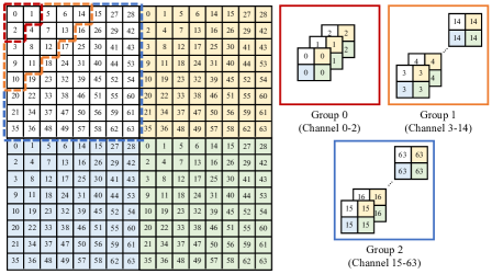
Figure 4: An example of frequency partitioning proposed in this paper. The left of this figure shows four adjacent blocks of $8\times 8$ DCT coefficients of luminance (Y plane), where the indices of coefficients follow the Zig-Zag scanning of JPEG. In this example, the 64 coefficients are partitioned into 3 groups according to frequency. In each group, the spatial position of the adjacent blocks is maintained, while coefficients of different coefficients is arranged across channels. Thus, the three groups in this figure have the shapes $2\times 2\times 3$, $2\times 2\times 12$, and $2\times 2\times 49$.

4 Frequency Partitioning

In this section, we further validate the efficiency of frequency partitioning in the proposed framework.

4.1 Correlation Across Frequencies

channels	bpsp	channels	bpsp	channels	bpsp
				[0, 3)	0.1227
		[0, 9)	0.2559	[3, 9)	0.1481
				[9, 18)	0.1822
				[18, 30)	0.1937
[0, 45)	0.8186	[9, 45)	0.5453	[30, 45)	0.1810
	0.8186		0.8012		0.8277

Table 1: The bits for grouped channels of kodim01. The number of channels $[m,n)$ is the index of $192$ frequency bands from $m$ to $n$. And bpsp is the bit per sub-pixel. The last line is the sum of each component.

First, we compare the compression performance with three grouping strategies. The first 45 channels in the arranged DCT coefficients $x$ are utilized in this experiment. As shown in Table 1, the 45 channels are split into 1/2/5 groups at different refinement levels. The best compression performance is achieved when the 45 channels are split into 2 groups. The reasons for that are of two aspects. First, the DCT coefficients are locally correlated. Second, the average intensities of different channels are distinguished. For example, the average intensity of channel 0 (DC) can be hundreds of times higher than channel 30-45, which may hinder the network from finding an optimum.

Moreover, we visualize the DCT coefficients with binary map of Y, Cb, Cr color planes to depict the correlation among low frequency components in Figure 5. Figure 5 is the most significant bit (MSB) map of 0-3 channels of the first 45 channels, which suggests high correlation in channel 0 across different color planes and some implicit correlation among other low frequency channels.

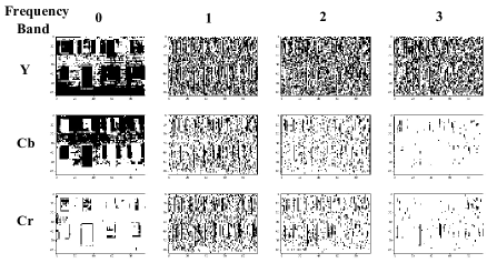
Figure 5: The most significant bit map of channel 0-3 of Y, Cb and Cr planes.

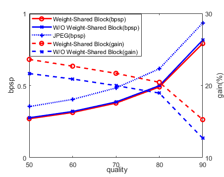
Figure 6: The ablation experiment of Weight-Shared Block on Kodak. The left y axis is bpsp, and the right is the compression ratio. Then red lines are the model with weight-shared block, while the blue dotted lines are the model without weight-shared block.

4.2 Frequency Partitioning Strategy

Based on the experiments and channel correlation introduced in Section 4.1, we split the $192$ channels into three groups. To illustrate the physical meaning of such partitioning strategy, we illustrate it in the original block DCT domain in Figure 4. For gray-scale image with only luminance (Y) plane, the 64 channels that indexed in Zig-Zag order are split into 3 groups: $[0,3),[3,15),[15,64)$. As for color images, the channels are grouped to $[0,9),[9,45),[45,192)$, where the color planes are ordered as Y$\rightarrow$Cb$\rightarrow$Cr$\rightarrow$Y$\rightarrow$Cb$\rightarrow$Cr$\cdots$.

Methods		Kodak_50	Kodak_60	Kodak_70	Kodak_80	Kodak_90
Baseline	JPEG	0.354	0.404	0.483	0.616	0.933	Average Gain to JPEG(%)	Average Gain to Others(%)
Learned	proposed	0.270(23.622)	0.313(22.682)	0.378(21.691)	0.490(20.447)	0.791(15.275)	20.743	-
	LZMA	0.345(2.344)	0.398(1.462)	0.480(0.553)	0.617(-0.162)	0.939(-0.661)	0.707	+20.036
	mozjpeg	0.324(8.287)	0.377(6.825)	0.456(5.600)	0.586(4.844)	0.881(5.553)	6.222	+14.521
	Brunsli	0.271(23.272)	0.317(21.681)	0.385(20.220)	0.500(18.903)	0.761(18.479)	20.511	+0.232
Handcrafted Methods	Lepton	0.265(25.159)	0.309(23.564)	0.377(21.972)	0.491(20.286)	0.756(18.931)	21.982	-1.249

Table 2: Compression performance on Kodak by our method, baseline (JPEG) methods, and existing handcrafted methods in terms of bits per sub-pixel (bpsp). We emphasize the difference in percentage to our approach for each other method in red if our method outperforms the other method and in green otherwise. For Kodak_m, $m$ is the quality factor to control the quality of JPEG images.

Methods		Set5_50	Set5_60	Set5_70	Set5_80	Set5_90
Baseline	JPEG	0.454	0.516	0.611	0.767	1.108	Average Gain to JPEG (%)	Average Gain to Others (%)
Learned	proposed	0.343(24.449)	0.391(24.258)	0.467(23.472)	0.596(22.271)	0.918(17.153)	22.321	-
	lzma	0.450(0.871)	0.514(0.476)	0.610(0.140)	0.767(-0.101)	1.112(-0.330)	0.211	+22.11
	mozjpeg	0.434(4.507)	0.494(4.348)	0.582(4.632)	0.724(5.612)	1.023(7.636)	5.347	+16.974
	Brunsli	0.362(20.202)	0.413(19.95)	0.516(19.417)	0.615(19.76)	0.882(20.388)	19.943	+2.378
Handcrafted Methods	Lepton	0.354(20.055)	0.405(21.628)	0.481(21.184)	0.606(20.946)	0.874(21.108)	20.984	+1.437

Table 3: Compression performance on Set5 by our method, baseline(JPEG), and existing handcrafted methods in terms of bits per sub-pixel (bpsp). We emphasize the difference in percentage to our approach for each other method in red if our method outperforms the other method and in green otherwise. For Set_m, $m$ is the quality factor to control the quality of JPEG images.

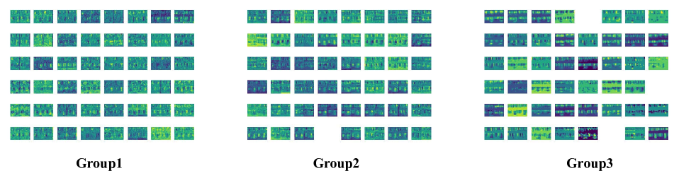
Figure 7: The visualization of features from frequency learning for the JPEG format of kodim01. The blank in group $2$ and $3$ is the redundant channel, which can not learn from input.

5 Experiments

5.1 Dataset

To train and test our neural network, we process the training and testing data according to the Figure 1. Moreover, We must obtain DCT coefficients from JPEG images, here we follow the code to get the quantization table and coefficients. Then the training dataset is DCT coefficients of Flickr data[4]. Firstly we crop these JPEG images with $256\times 256$, and then the input is $32\times 32$ since the DCT is $8\times 8$. Besides the training image batch is $4$. And the testing dataset is Kodak[3] and Set5[13]. We just transfer lossless format PNG as JPEG by controlling the quality factor with library ”jpeg-9c”. The set of quality factor is ${50,60,70,80,90}$, and $50$ means the worst quality and $90$ otherwise. It covers the commonly used quality for JPEG. Moreover the main memory cost of cloud and local machine is mainly from the JPEG images with high quality. And then we process testing data with the method same as the training data.

5.2 Training Strategies

We utilize Adam[27] optimizer to train our whole network with one GPU for two days. From the loss function in Equation (3.1), we train our neural network by balancing the rate of DCT coefficients and extracted features. To obtain higher compression ratio, we adjust the vaule of $\lambda$ during training instead of a constant value. Firstly we set small value for it, like $0.001$, then when training at 1M steps, we set a bit higher value, like $0.01$. At last, we set $\lambda=1$ for the last 1M step. Meanwhile, we adjust the learning rate by the exponential decay with $0.9$ until 10M steps.

5.3 Visualization of Features

To verify the frequency learning for lossless compression, we visualize the features that neural network learn from DCT coefficients. From the Figure 7, different frequency bands obtain different features. Neural network learns about the smoothed pixels from low frequecny as in Group1 in Figure 7 and learns about dramatically changing pixels as in Group3, like the edge and contours. Besides, since larger part of high frequency of DCT coefficients is zero, there exist some redundant feature channels in Group2 and Group3. It is the truth that the neural network can learn form DCT coefficients as the original RGB images, since DCT is reversible. Namely, CNN can learn from the inverse DCT. So we can infer the learning process, firstly it transforms the DCT coefficients into RGB images, and then learn the image pattern as the previous network. More importantly, neural network can learn from part frequency bands instead of all DCT coefficients. Since here is the lossless compression, we must process all frequency bands.

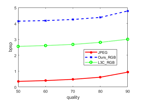
Figure 8: Learned methods with RGB input for JPEG images. We use the pretrained model L3C with green line. We use the learning methods with the same structure of Figure2 at blue line. The last red line is the baseline of JPEG image.

5.4 Results

We achieve more than 20% compression gain for JPEG images, as shown in Tables 2 and 3. Our compression performance outperforms LZMA about $20\%$ and mozjpeg about $15\%$, and it is comparable to Brunsli and Lepton. Besides, our method even has higher compression gain for the dataset Kodak_80 with $20.447\%$ to $20.286\%$. And we have higher compression ratio on Set5 dataset even for Brunsli and Lepton with $2.378\%$ and $1.437\%$ gain.

5.5 Ablation Studies

5.5.1 DCT vs. RGB

To verify the efficiency of learning in frequrency domain, we conduct the experiments with the RGB input. And Figure 8 shows all leaning in RGB has higher bpsp than the original images. Namely, they have no compression gain for JPEG images, though L3C has better performance in image with lossless format (BPG, JPEG2000 and so on). Besides we train our structure with the JPEG images, and test on Kodak dataset, its performance is far more worse than JPEG. To achieve lossless compression, neural network learn from each pixel and allocate its probability. Thus neural network can not identify whether the input image is lossless format. And that is our key motivation for learning in frequency domain.

5.5.2 Number of Groups

To explore the variable about the number of group, we set the following experiments. We split the whole $192$ channels into $1,2,3,4$ groups. When it is $1$ group, we have the whole frequency bands $[0,192)$ to jointly process these DCT coefficients. And experiments with $2$ groups has $[0,9),[9,192)$ frequency bands, and $3$ groups has $[0,9),[9,45),[45,192)$ , and $4$ groups has $[0,9),[9,45),[45,108),[108,192)$, respectively. We split these groups according to the Zig-Zag order of $8\times 8$ DCT, and it corresponds to super low, low, middle and high frequency. From the Figure 9 a single model can not achieve best performance for all qualities. More groups also do not have better compression ratio as the model with $4$ groups is worse than model with $2$ group for all qualities. To be mentioned, model with $2$ groups has the best performance at quality $90$ with regard to other models. We finally use model with three groups for testing because it has the best average performance.

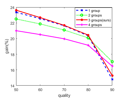
Figure 9: Compression gain of models with $1,2,3,4$ groups, respectively.

Group Number	1	2	3	4
Kodak_50	0.271	0.274	0.270	0.279
Kodak_60	0.313	0.316	0.313	0.321
Kodak_70	0.378	0.381	0.378	0.386
Kodak_80	0.490	0.492	0.490	0.498
Kodak_90	0.795	0.774	0.791	0.779

Table 4: Compression performance about bpsp of models with $1,2,3,4$ groups, respectively.

5.5.3 Weight-Shared Block

We conduct the experiments to verify the effectiveness of weight-shared block and the results are shown in Figure 6. Specifically, we disconnect the back flow in Figure 3($a$) to train the whole network with the same configuration. And it actually improves the performance by 2% for images across all qualities.

6 Conclusion and Discussion

As far as we know, we are the first to utilize deep learning method on frequency domain for lossless compression. The DCT coefficients are partitioned into several groups for efficient compression, which is based on the observation that DCT coefficients have implicit local correlation. Thus, joint processing adjacent channels can improve the lossless compression performance. Besides, different from the autoencoder with the symmetrical structure, we introduce the extra module for the decoder, such as weight-shared block, because the pattern of DCT coefficient is hard to capture, especially the altering coefficients. Finally we achieve the comparable performance to other traditional non-learned methods. Different from the rate-distortion loss $R+\lambda D$ for lossy compression, lossless compression has no distortion. In this paper, we just optimize the rate of input DCT coefficients and the extracted priors. However we also introduce the Lagrange factor $\lambda$ to balance the rate of each part.

References

- [1] The berkeley segmentation dataset and benchmark. https://www2.eecs.berkeley.edu/Research/Projects/CS/vision/bsds/.
- [2] Brunsli - github. https://github.com/google/brunsli.
- [3] Kodak lossless true color image suite (pho-tocd pcd0992). http://www.tp-ontrol.hu/index.php/TP_Toolbox.
- [4] Mirflickr. http://press.liacs.nl/mirflickr/mirflickr1m/.
- [5] Mozilla mozjpeg. https://blog.mozilla.org/research/2014/03/05/introducing-the-mozjpeg-project/.
- [6] Alvin Alpher. Frobnication. Journal of Foo, 12(1):234–778, 2002.
- [7] Alvin Alpher and Ferris P. N. Fotheringham-Smythe. Frobnication revisited. Journal of Foo, 13(1):234–778, 2003.
- [8] Alvin Alpher, Ferris P. N. Fotheringham-Smythe, and Gavin Gamow. Can a machine frobnicate? Journal of Foo, 14(1):234–778, 2004.
- [9] Seyed Mehdi Ayyoubzadeh and Xiaolin Wu. Lossless compression of mosaic images with convolutional neural network prediction. arXiv preprint arXiv:2001.10484, 2020.
- [10] J. Ballé, V. Laparra, and E. P. Simoncelli. End-to-end optimized image compression. In Proceedings of the 5th International Conference on Learning Representations, Toulon, France, April 2017.
- [11] J. Ballé, D. Minnen, S. Singh, S. J. Hwang, and N. Johnston. Variational image compression with a scale hyperprior. In Proceedings of the 6th International Conference on Learning Representations, Vancouver, BC, Canada, April 2018.
- [12] F. Bellard. BPG image format. https://bellard.org/bpg/.
- [13] Marco Bevilacqua, Aline Roumy, Christine Guillemot, and Marie Line Alberi-Morel. Low-complexity single-image super-resolution based on nonnegative neighbor embedding. 2012.
- [14] Krzysztof Blaszczyk, Peter Rossmanith, Dipl-Inf Alexander Langer, and Dipl-Inf Felix Reidl. Paq compression algorithm. 2012.
- [15] Sheng Cao, Chao-Yuan Wu, and Philipp Krähenbühl. Lossless image compression through super-resolution. arXiv preprint arXiv:2004.02872, 2020.
- [16] Yunpeng Chen, Haoqi Fan, Bing Xu, Zhicheng Yan, Yannis Kalantidis, Marcus Rohrbach, Shuicheng Yan, and Jiashi Feng. Drop an octave: Reducing spatial redundancy in convolutional neural networks with octave convolution. In Proceedings of the IEEE International Conference on Computer Vision, pages 3435–3444, 2019.
- [17] Zhengxue Cheng, Heming Sun, Masaru Takeuchi, and Jiro Katto. Learned lossless image compression with a hyperprior and discretized gaussian mixture likelihoods. In ICASSP 2020-2020 IEEE International Conference on Acoustics, Speech and Signal Processing (ICASSP), pages 2158–2162. IEEE, 2020.
- [18] Jinyoung Choi and Bohyung Han. Task-aware quantization network for jpeg image compression. In European Conference on Computer Vision, pages 309–324. Springer, 2020.
- [19] Jia Deng, Wei Dong, Richard Socher, Li-Jia Li, Kai Li, and Li Fei-Fei. Imagenet: A large-scale hierarchical image database. In 2009 IEEE conference on computer vision and pattern recognition, pages 248–255. Ieee, 2009.
- [20] Max Ehrlich, Larry Davis, Ser-Nam Lim, and Abhinav Shrivastava. Quantization guided jpeg artifact correction. In Proceedings of the European Conference on Computer Vision. Springer, 2020.
- [21] Max Ehrlich and Larry S. Davis. Deep residual learning in the jpeg transform domain. In Proceedings of the IEEE/CVF International Conference on Computer Vision (ICCV), October 2019.
- [22] Felix A Gers, Jürgen Schmidhuber, and Fred Cummins. Learning to forget: Continual prediction with lstm. 1999.
- [23] Mohit Goyal, Kedar Tatwawadi, Shubham Chandak, and Idoia Ochoa. Deepzip: Lossless data compression using recurrent neural networks. arXiv preprint arXiv:1811.08162, 2018.
- [24] Lionel Gueguen, Alex Sergeev, Ben Kadlec, Rosanne Liu, and Jason Yosinski. Faster neural networks straight from jpeg. In S. Bengio, H. Wallach, H. Larochelle, K. Grauman, N. Cesa-Bianchi, and R. Garnett, editors, Advances in Neural Information Processing Systems, volume 31. Curran Associates, Inc., 2018.
- [25] Kaiming He, Xiangyu Zhang, Shaoqing Ren, and Jian Sun. Deep residual learning for image recognition. In Proceedings of the IEEE conference on computer vision and pattern recognition, pages 770–778, 2016.
- [26] Daniel Reiter Horn, Ken Elkabany, Chris Lesniewski-Lass, and Keith Winstein. The design, implementation, and deployment of a system to transparently compress hundreds of petabytes of image files for a file-storage service. In 14th USENIX Symposium on Networked Systems Design and Implementation (NSDI 17), pages 1–15, 2017.
- [27] Diederik P Kingma and Jimmy Ba. Adam: A method for stochastic optimization. arXiv preprint arXiv:1412.6980, 2014.
- [28] Friso H Kingma, Pieter Abbeel, and Jonathan Ho. Bit-swap: Recursive bits-back coding for lossless compression with hierarchical latent variables. arXiv preprint arXiv:1905.06845, 2019.
- [29] M. Li, W. Zuo, S. Gu, D. Zhao, and D. Zhang. Learning convolutional networks for content-weighted image compression. In 2018 IEEE/CVF Conference on Computer Vision and Pattern Recognition, pages 3214–3223, Salt Lake City, UT, USA, June 2018.
- [30] Zhijing Li, Christopher De Sa, and Adrian Sampson. Optimizing jpeg quantization for classification networks. In Resource-Constrained Machine Learning (ReCoML) Workshop of MLSys 2020 Conference, Austin, TX, USA, 2020.
- [31] Z. Liu, T. Liu, W. Wen, L. Jiang, J. Xu, Y. Wang, and G. Quan. Deepn-jpeg: A deep neural network favorable jpeg-based image compression framework, 2018.
- [32] Fabian Mentzer, Eirikur Agustsson, Michael Tschannen, Radu Timofte, and Luc Van Gool. Practical full resolution learned lossless image compression. In Proceedings of the IEEE Conference on Computer Vision and Pattern Recognition, pages 10629–10638, 2019.
- [33] F. Mentzer, E. Agustsson, M. Tschannen, R. Timofte, and L. Van Gool. Conditional probability models for deep image compression. In 2018 IEEE/CVF Conference on Computer Vision and Pattern Recognition, pages 4394–4402, Salt Lake City, UT, USA, June 2018.
- [34] Fabian Mentzer, Luc Van Gool, and Michael Tschannen. Learning better lossless compression using lossy compression. In Proceedings of the IEEE/CVF Conference on Computer Vision and Pattern Recognition, pages 6638–6647, 2020.
- [35] D. Minnen, J. Ballé, and G. D. Toderici. Joint autoregressive and hierarchical priors for learned image compression. In Advances in Neural Information Processing Systems 31, pages 10771–10780, Montreal, QC, Canada, December 2018.
- [36] Full Author Name. The frobnicatable foo filter, 2014. Face and Gesture submission ID 324. Supplied as additional material fg324.pdf.
- [37] Full Author Name. Frobnication tutorial, 2014. Supplied as additional material tr.pdf.
- [38] Igor Pavlov. 7z format. http://www.7-zip.org/7z.html, 2019.
- [39] Han Qiu, Qinkai Zheng, Gerard Memmi, Jialiang Lu, Meikang Qiu, and Bhavani Thuraisingham. Deep residual learning-based enhanced jpeg compression in the internet of things. IEEE Transactions on Industrial Informatics, 17(3):2124–2133, 2020.
- [40] Majid Rabbani. Jpeg2000: Image compression fundamentals, standards and practice. Journal of Electronic Imaging, 11(2):286, 2002.
- [41] O. Rippel and L. Bourdev. Real-time adaptive image compression. In Proceedings of the 34th International Conference on Machine Learning, pages 2922–2930, Sydney, NSW, Australia, August 2017.
- [42] Thomas Sikora. Mpeg digital video-coding standards. IEEE signal processing magazine, 14(5):82–100, 1997.
- [43] L. Theis, W. Shi, A. Cunningham, and F. Huszár. Lossy image compression with compressive autoencoders. In Proceedings of the 5th International Conference on Learning Representations, Toulon, France, April 2017.
- [44] G. Toderici et al. Variable rate image compression with recurrent neural networks. In Proceedings of the 4th International Conference on Learning Representations, San Juan, Puerto Rico, May 2016.
- [45] A. van den Oord et al. Conditional image generation with PixelCNN decoders. In Advances in Neural Information Processing Systems 29, pages 4790–4798, Barcelona, Spain, December 2016.
- [46] A. van den Oord, N. Kalchbrenner, and K. Kavukcuoglu. Pixel recurrent neural networks. In Proceedings of the 33rd International Conference on Machine Learning, pages 1747–1756, New York, NY, USA, June 2016.
- [47] Gregory K Wallace. The jpeg still picture compression standard. Communications of The ACM, 34(4):30–44, 1991.
- [48] Kai Xu, Minghai Qin, Fei Sun, Yuhao Wang, Yen-kuang Chen, and Fengbo Ren. Learning in the frequency domain. arXiv preprint arXiv:2002.12416, 2020.
- [49] Xin Yuan and Raziel Haimi-Cohen. Image compression based on compressive sensing: End-to-end comparison with jpeg. IEEE Transactions on Multimedia, 22(11):2889–2904, 2020.