A Formal Metareasoning Model of Concurrent Planning and Execution

Abstract

Agents that plan and act in the real world must deal with the fact that time passes as they are planning. When timing is tight, there may be insufficient time to complete the search for a plan before it is time to act. By commencing execution before search concludes, one gains time to search by making planning and execution concurrent. However, this incurs the risk of making incorrect action choices, especially if actions are irreversible. This tradeoff between opportunity and risk is the problem addressed in this paper. Our main contribution is to formally define this setting as an abstract metareasoning problem. We find that the abstract problem is intractable. However, we identify special cases that are solvable in polynomial time, develop greedy solution algorithms, and, through tests on instances derived from search problems, find several methods that achieve promising practical performance. This work lays the foundation for a principled time-aware executive that concurrently plans and executes.

1 Introduction

In the real world, time passes as agents plan. For example, an agent that needs to get to the airport may have two options: take a taxi or ride a commuter train. Each of these options can be thought of as a partial plan to be elaborated into a complete plan before execution can start. Clearly, the agent’s planner should only elaborate the partial plan that involves the train if that can be done before the train leaves. Note, however, that in general this may require delicate scheduling of search effort across multiple competing partial plans. Elaborating the example, suppose the planner has two partial plans that are each estimated to require five minutes of computation to elaborate into complete plans. If only six minutes remain until they both expire, then we would want the planner to allocate almost all of its remaining planning effort to one of them, rather than to fail on both. Issues like these have been the focus of previous work on situated temporal planning (Cashmore et al. 2018; Shperberg et al. 2019).

In this paper, we consider the design of a bolder agent that can begin execution of actions before a complete plan to a goal has been found. Consider a further extension of the example in which the estimated time to complete each plan is seven minutes. The only apparent way to achieve the agent’s goal thus involves starting to act before planning is complete. However, when an action is executed, plans that are not consistent with this action may become invalid, thus incurring the risk of never reaching the goal. This risk is most significant when actions are irreversible. However, even when an action can be reversed, the time spent executing a reversible action (and potentially its inverse action) might still cause the invalidation of plans. For example, taking the commuter train invalidates the partial plan of taking a taxi, as there will not be enough time to take the train in the opposite direction to still catch the taxi and reach the airport before the deadline. Thus, if the planner fails to elaborate the partial plan of riding the train into a complete plan that reaches the airport on time, the agent will miss its flight. This paper proposes a disciplined method for making execution decisions while handling such tradeoffs when allocating search effort in situated planning.

The idea of starting to perform actions in the real world (also known as base-level actions) before completing the search goes back at least as far as Korf’s (1990) real-time A*. The difference from the real-time search setting is that our scenario is more flexible: the agent does not have a predefined time at which the next action must be executed. Rather, it can choose when base-level actions should be executed in order to maximize the probability of successful and timely execution. Note that we assume that the world is deterministic. The only uncertainty we model concerns how long planning will take and the time it will take the as-yet-unknown resulting plan to reach a goal state, i.e., we only consider uncertainty at the meta-level. Our setting is also different from the interleaving of planning and execution in order to account for stochastic actions or partial observability, which has been a part of practical applications of planning since the early days of Shakey the robot (Fikes, Hart, and Nilsson 1972) and later (e.g., Ambros-Ingerson, Steel et al. (1988); Haigh and Veloso (1998); Lemai and Ingrand (2004); Nourbakhsh (1997)).

Our main contribution is defining the above issues as a formal problem of decision-making under uncertainty, in the sense defined by Russell and Wefald (1991). Attempting this formalization for a full realistic search algorithm appears daunting, even under our assumption of a deterministic world. We thus begin from the formal (AE)² model (for Allocating Effort when Actions Expire) of Shperberg et al. (2019), which formalizes situated planning as an abstract metareasoning problem of allocating processing time among $n$ search processes (e.g., subtrees). The objective is to find a policy that maximizes the probability of finding a solution plan that is still feasible to execute when it is found. We extend the model to allow execution of actions in the real world in parallel with the search processes. We call this model Concurrent Planning and Execution (CoPE for short).

CoPE is a generalization of (AE)², so finding an optimal CoPE policy is also intractable, even under the assumption of known deadlines and remainders. Still, we cast CoPE as an MDP, so that we can define and analyze optimal policies, and even solve CoPE optimally for very small instances using standard MDP techniques like value iteration. We then describe several efficient suboptimal ways of solving CoPE and evaluate them empirically. We find that our algorithms span a useful range of speed / effectiveness trade-offs.

This paper examines the static version of the metareasoning problem, i.e. solving the CoPE instance as observed at a snapshot of the planning process. Using our results in a temporal planner would likely involve gathering the requisite statistics and solving CoPE repeatedly, possibly after each node expansion. These integration issues are important future work that is beyond the scope of the current paper.

2 Background

In situated temporal planning (Cashmore et al. 2018), each possible action $a$ (i.e., an action in the search tree that the agent can choose whether to execute or not) has a latest start time $t_{a}$ and a plan must be fully generated before its first action can begin executing. This induces a planning deadline which might be unknown, since the actions in the plan are not known until the search terminates. For a partial plan available at a search node $i$ in the planner, the unknown deadline by which any potential plan expanded from node $i$ must start executing can be modeled by a random variable. Thus, the planner faces the metareasoning problem of deciding which nodes on the open list to expand in order to maximize the chance of finding a plan before its deadline.

Shperberg et al. (2019) propose the (AE)² model, which abstracts away from the search details and merely posits $n$ independent ‘processes.’ Each process is attempting to solve the same problem under time constraints. In the context of situated temporal planning using heuristic search, each process may represent a promising partial plan for the goal, implemented as a node on the open list, where the allocation of CPU time to that process is equivalent to the exploration of the subtree under the corresponding node. But the abstract problem may also be applicable to other settings, such as algorithm portfolios or scheduling candidates for job interviews. The metareasoning problem is to determine how to schedule the $n$ processes.

When process $i$ terminates, it delivers a solution with probability $P_{i}$ or, otherwise, indicates its failure to find one. As mentioned above, each process has an uncertain deadline, defined over absolute wall-clock time, by which its computation must be completed in order for any solution it finds to be valid. For process $i$, $D_{i}(t)$ denotes the CDF over wall clock times of the random variable denoting the latest start time (deadline). This value is only discovered with certainty when the process completes. This models the fact that a plan’s dependence on an external timed event, such as a train departure, might not become clear until the final action in a plan is added. If a process terminates with a solution before its deadline, it is called timely. Given $D_{i}(t)$, one can assume w.l.o.g. that $P_{i}$ is 1, otherwise adjust $D_{i}(t)$ to make the probability of a deadline that is in the past (thus forcing the plan to fail) equal to $1-P_{i}$.

The processes have known search time distributions, i.e. performance profiles (Zilberstein and Russell 1996) described by CDFs $M_{i}(t)$, the probability that process $i$ needs total computation time $t$ or less to terminate. As is typical in metareasoning, (AE)² assumes that all the random variables are independent. Given the $D_{i}(t)$ and $M_{i}(t)$ distributions, the objective of (AE)² is to schedule processing time between the $n$ processes such that the probability of at least one process finding a timely solution is maximized.

A simplified discrete-time version of the problem, called S(AE)², was cast as a Markov decision process. The MDP’s actions are to assign (schedule) the next time unit to process $i$, denoted by $c_{i}$ with $i\in[1,n]$. Computational action $c_{i}$ is allowed only if process $i$ has not already failed. A process is considered to have failed if it has terminated and discovered that its deadline has already passed, or if the current time is later than the last possible deadline for the process. Transitions are determined by the probabilistic performance profile $M_{i}$ and the deadline distributions (see Shperberg et al. (2019) for details). A process terminating with a timely solution results in success and a reward of 1.

Example 1: We need to get to terminal C at the airport 30 minutes from now. Two partial plans are being considered: riding a commuter train or taking a taxi. The train leaves in six minutes and takes 22 minutes to reach the airport. The planner has not yet determined how to get to terminal C: it may require an additional ten minutes using a bus (with probability 0.2), or the terminals may be adjacent, requiring no transit time. The taxi plan entails calling a taxi (2 minutes), then a ride taking 20 minutes to get to airport terminal C, and finally a payment step, the type and length of which the planner has not yet determined (say one or ten minutes, each with probability 0.5). Suppose the remaining planning time for the train plan is known to be eight minutes with certainty, and for the taxi plan it is distributed: $[0.5:4;0.5:8]$.

This scenario is modeled in S(AE)² as follows. We have two processes: process 1 for the plan with the commuter train with $m_{1}=[1:8]$ and process 2 for the taxi plan with $m_{2}=[0.5:4;0.5:8]$, where we show the PMF $m_{i}$ rather than the CDF $M_{i}$ for clarity. The deadline distribution PMFs are: $d_{1}=[0.2:-1,0.8:6]$: fail with probability 0.2 (the train plus bus plan arrives at terminal C at time 38, which does not meet our goal of 30) and six minutes with probability 0.8 (the train only plan) and $d_{2}=[0.5:-1,0.5:7]$.

Allocating planning time equally fails with certainty: neither process terminates in time to act. The optimal S(AE)² policy realizes that process 1 cannot deliver a timely solution ($d_{1}$ is less than $m_{1}$ with probability 1) and allocates all processing time to process 2, hoping it will terminate in 4 minutes and find a payment plan that takes only one minute, resulting in success with probability $0.5\times 0.5=0.25$.

2.1 Greedy Schemes

As solving the metareasoning problem is NP-hard, Shperberg et al. (2019) and Shperberg et al. (2021) used insights from a diminishing returns result to develop greedy schemes. Their analysis is restricted to linear contiguous allocation policies: schedules where the action taken at time $t$ does not depend on the results of the previous actions, and where each process receives its allocated time contiguously.

Following their notation, we denote the probability that process $i$ finds a timely plan when allocated $t_{i}$ consecutive time units beginning at time $t_{b_{i}}$ as:

$$s_{i}(t_{i},t_{b_{i}})=\sum_{t^{\prime}=0}^{t_{i}}(M_{i}(t^{\prime})-M_{i}(t^{\prime}-1))(1-D_{i}(t^{\prime}+t_{b_{i}}))$$ (1)

For linear contiguous policies, we need to allocate $t_{i}$, $t_{b_{i}}$ pairs to all processes (with no allocation overlap). Overall, a timely plan is found if at least one process succeeds, that is, overall failure occurs only if all processes fail. Therefore, in order to maximize the probability of overall success (over all possible linear contiguous allocations), we need to allocate $t_{i}$, $t_{b_{i}}$ pairs so as to maximize the probability:

$$P_{s}=1-\prod_{i}(1-s_{i}(t_{i},t_{b_{i}}))$$ (2)

Using $LPF_{i}(\cdot)$ (‘logarithm of probability of failure’) as shorthand for $log(1-s_{i}(\cdot))$, we note that $P_{s}$ is maximized if the sum of the $LPF_{i}(t_{i},t_{b_{i}})$ is minimized and that $-LPF_{i}(t_{i},t_{b_{i}})$ behaves like a utility that we need to maximize. For known deadlines, we can assume that no policy will allocate processing time after the respective deadline. We will use $LPF_{i}(t)$ as shorthand for $LPF_{i}(t,0)$.

To bypass the problem of non-diminishing returns, the notion of most effective computation time for process $i$ under the assumption that it begins at time $t_{b}$ and runs for $t$ time units was defined as:

$$e_{i}(t_{b})=\arg\!\min_{t}\frac{LPF_{i}(t,t_{b})}{t}$$ (3)

We use $e_{i}$ to denote $e_{i}(0)$ below.

Since not all processes can start at time 0, the intuition from the diminishing returns optimization is to prefer process $i$ that has the best utility per time unit, i.e. such that $-LPF_{i}(e_{i})/e_{i}$ is greatest. But allocating time to process $i$ delays other processes, so it is also important to allocate the time now to processes that have an early deadline. Shperberg et al. (2019) therefore suggested the following greedy algorithm (denoted as basic greedy scheme, or bgs for short): Iteratively allocate $t_{u}$ units of computation time to process $i$ that maximizes:

$$Q(i)=\frac{\alpha}{E[D_{i}]}-\frac{LPF_{i}(e_{i})}{e_{i}}$$ (4)

where $\alpha$ and $t_{u}$ are positive empirically determined parameters, and $E[D_{i}]$ is the expectation of the random variable that has the CDF $D_{i}$ (a slight abuse of notation). The $\alpha$ parameter trades off between preferring earlier expected deadlines (large $\alpha$) and better performance slopes (small $\alpha$).

The first part of Equation 4 is a somewhat ad-hoc measure of urgency that performs poorly if the deadline distribution has a high variance. A more precise notion of urgency was defined by Shperberg et al. (2021) as the damage caused to a process if its computation is delayed by some time $t_{u}$. This is based on the available utility gain after the delay of $t_{u}$. An empirically determined constant multiplier $\gamma$ was used to balance between exploiting the current process reward from allocating time to process $i$ now and the loss in reward due to delay. Thus, the delay-damage aware (DDA) greedy scheme was to assign, at each processing allocation round, $t_{u}$ time to the process $i$ that maximizes:

$$Q^{\prime}(i) =\frac{\gamma\cdot LPF_{i}(e_{i}(t_{u}),t_{u})}{e_{i}(t_{u})}-\frac{LPF_{i}(e_{i},0)}{e_{i}}$$ (5)

The DDA scheme was then adapted and integrated into the OPTIC temporal planner (Benton, Coles, and Coles 2012), providing state-of-the-art results on situated problems where external deadlines play a significant role (Shperberg et al. 2021).

2.2 DP Solution for Known Deadlines

For S(AE)² problems with known deadlines (denoted KDS(AE)²), it suffices to examine linear contiguous policies sorted by an increasing order of deadlines (Shperberg et al. 2019), formally:

Theorem 1.

Given a KDS(AE)² problem, there exists a linear contiguous schedule with processes sorted by a non-decreasing order of deadlines that is optimal.

Theorem 1 was used by Shperberg et al. (2021) to obtain a dynamic programming (DP) scheme:

Theorem 2.

For known deadlines, DP according to

$$\!OPT(t,l)=\!\max\limits_{0\leq j\leq d_{l}-t}\left(\!OPT(t\!+\!j,l\!+\!1)\!-\!LPF_{l}(j)\right)$$ (6)

finds the optimal schedule in time polynomial in $n$, $d_{n}$.

For explicit $M_{i}$ representations, evaluating Equation 6 in descending order of deadlines runs in polynomial time.

3 Concurrent Planning and Execution

Our new CoPE model extends the abstract $S(AE)^{2}$ model to account for possible execution of actions during search. We associate each process with a sequence of actions, representing the prefix of a possible complete plan below the node the process represents. For each process, there is a plan remainder that is still unknown. In the context of temporal planning, these assumptions are reasonable if we equate each process with a node in the open list of a forward-search algorithm that searches from the initial state to the goal and adds an action when a node is expanded. Here, the prefix is simply the list of operators leading to the current node. The rest of the action sequence is the remaining solution that may be developed in the future from each such node. However, here too we will abstract away from the actual search and model future search results by distributions. Thus, in addition to the $M_{i}$ distributions over completion times, for each process $i$ we have a unique plan prefix $H_{i}$ ($H$ for head), containing a sequence of actions from a set of available base-level actions $B$. Each action $b\in B$ also has a deadline $D(b)$. Upon termination, a process $i$ delivers the rest of the action sequence $\beta_{i}$ of the solution. As $\beta_{i}$ is unknown prior to termination, we model $dur(\beta_{i})$, the duration of $\beta_{i}$, by a random variable ${\cal R}_{i}$ whose value becomes known upon termination.

Unlike in previous work on situated temporal planning, which requires a complete plan before any action is executed, here actions from any action sequence $H_{i}$ may be executed (in sequence) even before having a complete plan. Execution changes the state of the system and we adjust the set of processes to reflect this: any process $i$ where the already executed action sequence is not a prefix of $H_{i}$ becomes invalid. An execution of any prefix of actions from any $H_{i}$ is legal if and only if: i) the first action starts no earlier than time 0 (representing the current time), ii) the next action in the sequence begins at or after the previous action terminates, and iii) every action is executed before its deadline. Each suffix $\beta_{i}$ is assumed to be composed of actions that cannot be executed before process $i$ terminates. Thus $start(\beta_{i})$, the time at which $\beta_{i}$ may begin execution, must be no earlier than the time at which process $i$ terminates. We also assume that base-level actions are non-preemptible and cannot be run in parallel. However, computation may proceed freely while executing a base-level action.

As in $S(AE)^{2}$, we have a deadline for each process, but with a different semantics: In $S(AE)^{2}$, a complete plan must be found in order to start execution. As a result, the deadline distribution in $S(AE)^{2}$ is defined over the latest possible time to start executing the entire plan. However, here the requirement is that the execution terminates before the (possibly unknown) deadline; we call a sequence of actions fully executed before its deadline a timely execution. Thus, the deadline distribution for CoPE is defined differently. We begin by assuming that there is a known distribution (of a random variable ${\cal X}_{i}$) over $deadline_{i}$, the deadline for process $i$, and again that its true value becomes known only once the search in process $i$ terminates. An execution of a solution delivered by process $i$ is timely just when the $start(\beta_{i})$ occurs in time to conclude before the process $i$ deadline; i.e. $start(\beta_{i})\leq{\cal X}_{i}-{\cal R}_{i}$. We call this value constraining $start(\beta_{i})$ the induced deadline for process $i$, and denote it by ${\cal D}_{i}$. Note that ${\cal D}_{i}={\cal X}_{i}-{\cal R}_{i}$ is well defined even if ${\cal R}_{i}$ and ${\cal X}_{i}$ are dependent. Thus, we will henceforth simply assume that the induced deadline ${\cal D}_{i}$ has a known distribution given by its CDF $D_{i}$ and we can ignore ${\cal X}_{i}$ and ${\cal R}_{i}$. So finally, for a process $i$ to be timely, it must meet two conditions: 1) complete its computation, and 2) complete execution of its entire action prefix $H_{i}$ before the induced deadline ${\cal D}_{i}$. In summary, we have:

Definition 1.

A Concurrent Planning and Execution problem (CoPE) is, given a set of base-level actions $B$ where each action $b\in B$ has duration $dur(b)>0$, $n$ processes, each with a (possibly empty) sequence $H_{i}$ of actions from $B$, a performance profile $M_{i}$, and the induced deadline distribution of each ${\cal D}_{i}$, to find a policy for allocating computation time to the $n$ processes and legally executing base-level actions from some $H_{i}$, such that the probability of executing a timely solution is maximal.

Example 2: Representing the scenario of example 1 (getting to terminal C in 30 minutes) in CoPE, we again have 2 processes with the same performance profiles as in S(AE)²: $m_{1}=[1:8]$, $m_{2}=[0.5:4;0.5:8]$. We also have $H_{1}=[\mbox{ride train}]$ and $H_{2}=[\mbox{phone, take taxi}]$, with $dur(\mbox{phone})=2$, $dur(\mbox{ride train})=22$, $dur(\mbox{take taxi})=20$, and the train leaves in six minutes. The remainder durations are distributed as follows. For $\beta_{1}$ we have ${\cal R}_{1}\sim[0.8:0~{};0.2:10]$, and for $\beta_{2}$ we have ${\cal R}_{2}\sim[0.5:1~{};~{}0.5:10]$. The deadlines are certain in this case, ${\cal X}_{1}={\cal X}_{2}=30$, and the induced deadlines are thus distributed: ${\cal D}_{1}\sim[0.8:30~{};0.2:20]$ and ${\cal D}_{2}\sim[0.5:29~{};0.5:20]$.

The optimal CoPE policy here is to run process 2 for four minutes. If it terminates and reveals that ${\cal D}_{2}=29$ then call for a taxi and proceed (successfully) with the taxi plan. Otherwise (process 2 does not terminate, or terminates and reveals that ${\cal D}_{2}=20$), start executing the action from $H_{1}$: take the train and run process 1, hoping to find that ${\cal D}_{1}=30$ (the train stops at terminal C). This policy works with probability of success $P_{S}=0.25+0.75*0.8=0.85$, as opposed to a success probability of $0.25$ for the optimal solution under S(AE)². Furthermore, had the terminal C arrival deadline been 25 minutes, all S(AE)² solutions would have had zero probability of success, while in the CoPE model it is possible to commit to taking the taxi even before planning is done, resulting in a probability of success $P_{S}=0.5$ (due to the yet unknown payment method).

We have seen how the added complexity of CoPE can pay off by enabling execution concurrently with planning. However, the problem setting remains well-defined and amenable to analysis. To analyze CoPE, we make four simplifying assumptions: 1) Time is discrete 2) The action durations $dur(b)$ are known for all $b\in B$. 3) The variables with distributions $D_{i}$, $M_{i}$ are all mutually independent. 4) The individual action deadlines $D(b)$ are irrelevant (not used, or equivalently set to be infinite), as the processes’ overall induced deadline distributions $D_{i}$ are given. Although assumption 4 is easy to relax (our implementation allows for individual action deadlines), doing so complicates the analysis.

3.1 Formulating CoPE as an MDP

We can state the CoPE optimization problem as the solution to an MDP similar to the one defined for $S(AE)^{2}$. The actions in the CoPE MDP are of two types: the actions $c_{i}$ that allocate the next time unit of computation to process $i$ as in $S(AE)^{2}$, to which CoPE adds the possibility to execute a base-level action from $B$. We assume that $c_{i}$ can only be done if process $i$ has not already terminated and has not become invalid (and thus fails) by execution of incompatible base-level actions. An action $b$ from $B$ can only be done when no other base-level action is currently executing and $b$ is the next action in some $H_{i}$ (after the common prefix of base-level actions that all remaining processes share).

The states of the MDP are defined as the cross product of the following state variables: (i) wall-clock (real) time $T$; (ii) the time $T_{i}$ already used by process $i$, for all $1\leq i\leq n$; (iii) for each process $i$, an indicator of whether it has failed; (iv) the time left $W$ until the current base-level action completes execution; and (v) the number $L$ of base-level actions already initiated or completed. We also have special terminal states SUCCESS (denoting having found and an executable timely plan) and FAIL (no longer possible to execute a timely plan). The identity of the base-level actions already executed is not explicit in the state, but can be recovered as the first $L$ actions in any prefix $H_{i}$, for a process $i$ not already failed. The initial state $S_{0}$ has elapsed wall-clock time $T=0$, no computation time used for any process, so $T_{i}=0$ for all $1\leq i\leq n$, and no base-level actions executed or started so $W=0$ and $L=0$. The reward function is 0 for all states, except SUCCESS, which has a reward of 1.

The transition distribution is straightforward (see appendix): deterministic except for computation actions $c_{i}$, which advance the wall-clock time, and additionally process $i$ terminates with probability $P_{C,i}=\frac{m_{i}(T_{i}[S]+1)}{1-M_{i}(T_{i}[S])}$ where $T_{i}[S]$ is the time already allocated to process $i$ before the current state $S$. Termination results in SUCCESS if the resulting plan execution can terminate before the (now known) deadline, otherwise the process is called failed. A process for which there is no chance for success is called tardy. We allow a computation action $c_{i}$ only for processes $i$ that have not failed and are not tardy at $S$. If all processes are either tardy or failed, we transition to the global FAIL state.

4 Known Induced Deadline CoPE

Any instance of $S(AE)^{2}$ can be made a CoPE instance by setting all $H_{i}$ to null. Thus finding the optimal solution to CoPE is also NP-hard, even under assumptions 1-4 and known induced deadlines $d_{i}$. We denote this known-induced-deadline restriction of CoPE by KID-CoPE and analyze this case, trying to get a pseudo-polynomial time algorithm for computing the optimal policy.

We can represent a policy as an and-tree rooted at the initial state $S_{0}$, with each of the agent’s actions as an edge from each state node, leading to a chance node with next possible states as children. A policy tree in which every chance node has at most one non-terminal child with non-zero probability is called linear, because it is equivalent to a simple sequence of meta-level and base-level actions.

Lemma 3.

In KID-CoPE all policies are linear.

The Proof of Lemma 3 can be found in the appendix.

In KID-CoPE it thus suffices to find the best linear policy, represented henceforth as a sequence $\sigma$ of the actions (both computational and base-level) to be done starting from the initial state and ending in a terminal state.

Denote by $CA(\sigma)$ the sub-sequence of $\sigma$ that contains just the computation actions. Likewise, $BA(\sigma)$ denotes the base-level actions. We call a linear policy contiguous if the computation actions for every process are all in contiguous blocks:

Definition 2.

Linear policy $\sigma$ is contiguous iff $CA(\sigma)[k_{1}]=CA(\sigma)[k_{2}]=c_{i}$ implies $CA(\sigma)[m]=c_{i}$ for all $k_{1}<m<k_{2}$ and all computation actions $c_{i}$.

Theorem 4.

In KID-CoPE, there exists an optimal policy that is linear and contiguous.

The proof of Theorem 4 can be found in the appendix.

We still need to schedule the base-level actions. We show that schedules we call lazy are non-dominated. Intuitively, a lazy policy is one where execution of base-level actions is delayed as long as possible without making the policy tardy or illegal (e.g., base-level actions overlapping). Denote by $\sigma_{i\leftrightarrow j}$ the sequence resulting from exchanging the $i$th and $j$th actions in $\sigma$.

Definition 3.

A linear policy $\sigma$ is lazy if $\sigma_{i\leftrightarrow i+1}$ is tardy or illegal for all $i$ where $\sigma[i]\in B$.

Theorem 5.

In KID-CoPE, there exists an optimal policy that is linear, contiguous, and lazy.

The proof of Theorem 5 can be found in the appendix.

5 Pseudo-Polynomial Time Algorithms

For KDS(AE)², there exists an optimal linear contiguous policy that assigns computations in order of deadline. Unfortunately, things are not so simple for CoPE because the timing of the base-level actions affects the order in which computation actions become tardy. However, if we fix the base-level execution start times we can then reduce the resulting KID-CoPE instance into a KDS(AE)² instance, which can be solved in pseudo-polynomial time using DP, as follows.

First, observe that the sequences of actions we need to consider are only the $H_{i}$, as any policy containing an action not in such a sequence would invalidate all the processes and thus is dominated. We call the mapping from $H_{i}$ to the action execution start times an initiation function for $H_{i}$, denoted by $I_{i}$. Note that a policy $\sigma$ with $BA(\sigma)=H_{i}$ may have computations from other processes $j$, up until such time as $j$ is invalidated by $\sigma$. Under a given initiation function $I_{i}$, we can define an effective deadline $d_{j}^{\text{eff}}(I_{i})$ for each process $j$, beyond which there is no point in allowing process $j$ to run. Note that the effective deadline is distinct from the known induced process deadline $d_{i}$.

To define the effective deadline, let $k\in H_{i}$ be the first index at which prefix $H_{j}$ becomes incompatible with $H_{i}$. Then process $j$ becomes invalid at time $I_{i}(k)$. Also, consider any index $m<k$ at which the prefixes are still compatible. The last time at which action $H_{i}[m]$ may be executed to achieve the known induced deadline $d_{j}$ is $t_{i,m}=d_{j}-dur(H_{j}[m..|H_{j}|])$. That is, process $j$ becomes tardy at $t_{i,m}$ unless base-level action $H_{i}[m]$ is executed before then. The effective deadline $d_{j}^{\text{eff}}$ for process $j$ is thus:

$$d_{j}^{\text{eff}}(I_{i})=\min_{m<k}(I_{i}(k),\{t_{i,m}:t_{i,m}<I_{i}(H_{i}[m])\})$$ (7)

Theorem 6.

Among the set of linear contiguous policies for a specific $H_{i}$ and initiation function $I_{i}$, there exists an optimal policy where the processes are allocated in order of non-decreasing effective deadlines.

The proof of Theorem 6 can be found in the appendix.

Given specific $H_{i}$ and $I_{i}$, the proof of Theorem 6 constructs an equivalent KDS(AE)² instance. This instance can be solved using DP to find the optimal computations policy and its success probability. Now simply iterating over the $n$ possible $H_{i}$ and all possible $I_{i}$, and taking the best (highest probability of success) KDS(AE)² solution, we get the optimal KID-CoPE policy. The catch is that in general, the number of initiation functions to consider is exponential. But in some cases, we can show that the number of such initiation functions we need to consider is small.

Bounded Length Prefixes:

If the length of all the $H_{i}$ is bounded by a constant $K$, we get a pseudo-polynomial time algorithm, because the number of initiation functions is at most $|dom(T)|^{|H_{i}|}$.

To implement this technique, we iterate over all possible initiation functions $I_{i}$ up to length $K$. If $H_{i}$ is longer than $K$, we complete $I_{i}$ using some default scheme, thereby giving up on optimality. This is what we do in the K-bounded scheme in the next section.

The equal slack case:

The difference $sl_{i}=d_{i}-dur(H_{i})$, the slack of process $i$, is the maximum time we can delay the actions in $H_{i}$ without making process $i$ tardy. The special case of KID-CoPE where the slack of all processes is equal affords the following pseudo-polynomial time algorithm. Let the slack of all processes equal $sl$. Consider any non-tardy linear contiguous policy $\sigma$ that has $BA(\sigma)=H_{i}$. Then $\sigma$ is lazy only if $I_{i}^{\sigma}(H_{i}[1])=sl$. In this case the actions in $H_{i}$ must be executed contiguously starting at $sl$, as otherwise $\sigma$ would be tardy. The resulting unique lazy $I_{i}$ is thus independent of $\sigma$ (as long as $BA(\sigma)=H_{i}$) and due to Theorem 5 is the only one we need to consider for each $H_{i}$.

To summarize this case, for each $H_{i}$ set the $d^{\text{eff}}_{j}(I_{i})$ for all processes assuming the unique lazy $I_{i}$ using Equation 7, solve the resulting KDS(AE)² instance, and pick the best of these $n$ solutions.

Note that having a known deadline entails a known induced deadline in problems with constant length solutions, such as CSPs. But in general (e.g., the 15-puzzle instances from our empirical evaluation) $dur(\beta_{i})$ is unknown before the solution is found, thus the induced deadline is also unknown. It is possible for process $i$ to find a solution, only to discover that it cannot be executed on time, even for known deadlines.

6 Algorithms for the General Case

While optimal, the pseudo-polynomial time algorithms in Section 5 only apply to known deadlines plus additional assumptions. We thus propose two categories of suboptimal schemes for the general case: a) focusing primarily on execution or b) focusing primarily on computation.

Execution-focused schemes choose some base-level action initiations. Effective deadlines are computed for each initiation, giving S(AE)² problem instances. Computations are allocated with any S(AE)² algorithm $A$. Specifically:

1) The Max-LET_A schema considers the minimal value in the support of $D_{i}$ for each $i$. (Other methods of fixing the deadline can be used, e.g. taking the expectation). Then, for every process $i$, Max-LET_A fixes the base-level actions to their Latest Execution-Time at which every action in the head must be executed (with respect to the known deadline). By fixing the base-level actions to those induced by process $i$, the CoPE problem instance is reduced to an S(AE)² instance. Then algorithm $A$ is executed on the S(AE)² instance and returns a linear policy $\pi_{i}$ and its success probability. Looking over each process’ $\pi_{i}$, Max-LET_A chooses the one with the highest success probability.

2) K-Bounded_A is similar to Max-LET_A with one difference. Instead of fixing base-level actions only to the latest start-time of every process $i$, K-Bounded_A considers all possible placements for the first $K$ actions. The rest (if any) of the time-allocations are determined using latest start-time.

Schemes focusing on computations treat a CoPE instance as if it were an S(AE)² instance, ignoring the base-level actions when allocating computation action(s). These schemes can use any S(AE)² algorithm to schedule computations. For example, Demand-Execution_A first decides which computation $c_{i}$ should be done in the next time unit using S(AE)² algorithm $A$, under the assumption that no base-level actions are executed before computation terminates. Then it checks whether a base-level action $b$ is required for $c_{i}$ to be non-tardy. If so, the base-level action $b$ is returned, otherwise $c_{i}$ is returned.

Hybrid approaches are also possible. We tried Monte-Carlo tree search (MCTS), which is applicable to any MDP (Browne et al. 2012). The MCTS version we used utilizes UCT (Kocsis and Szepesvári 2006), which applies the UCB1 formula (Auer, Cesa-Bianchi, and Fischer 2002) for selecting nodes, and a random rollout policy that uses $-LPF$ as a value function for sampled time allocations.

7 Empirical Evaluation

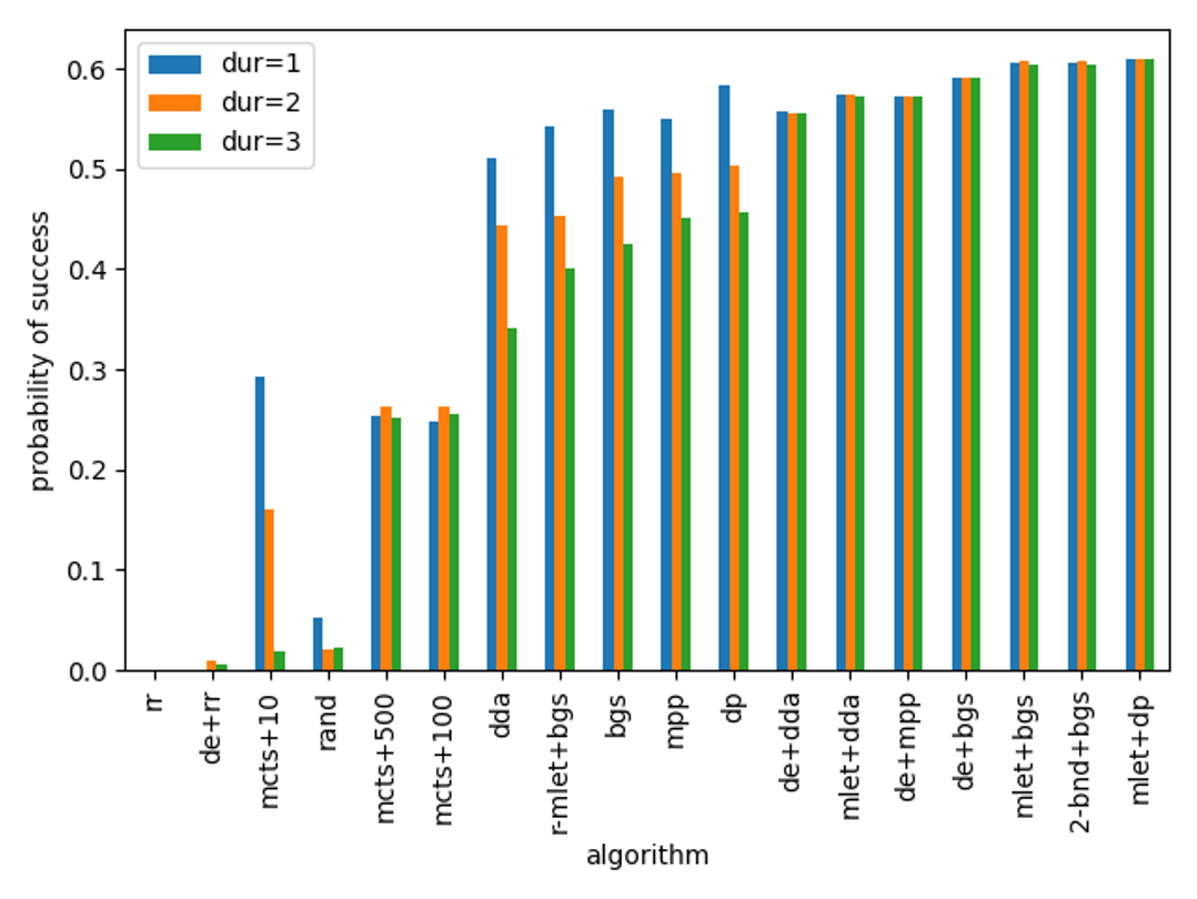
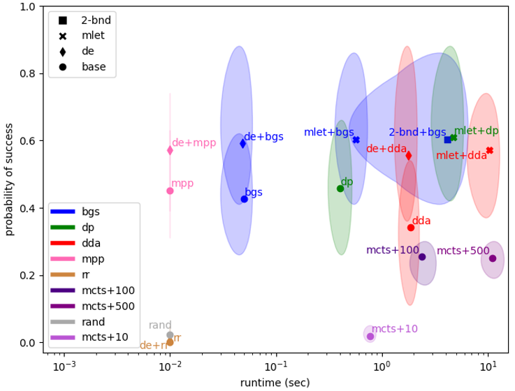
Figure 1: Results for 20 processes: top) average success probability, bottom) success vs runtime for $dur(b)=3$.

Our experimental setting is inspired by movies such as Indiana Jones or Die Hard in which the hero is required to solve a puzzle before a deadline or suffer extreme consequences. As the water jugs problem from Die Hard is too easy, we use the 15-puzzle with the Manhattan distance heuristic instead. We collected data by solving 10,000 15-puzzle instances, recording the number of expansions required by $A^{\ast}$ to find an optimal solution from each initial state, as well as the actual solution length. Then, two CDF histograms were created for each initial $h$-value: the required number of expansions, and the optimal solution lengths. CoPE problem instances of $N$ processes were generated by drawing a random 15-puzzle instance, running $A^{\ast}$ until the open-list contained at least $N$ search nodes, with $N\in\{2,5,10,20,50\}$, and then choosing the first $N$. Each open-list node $i$ became a CoPE process, with $M_{i}$ being the node-expansion CDF histogram corresponding to $h(i)$; ${\cal R}_{i}$ taken from the solution-cost histogram (to represent the remaining duration of the plan); and $H_{i}$ the list of actions that leads to $i$ from the start node. In this setting, all base-level actions require the same amount of time units to be completed, denoted as $dur(b)$; in our experiments, we considered $dur(b)\in\{1,2,3\}$ (i.e. each 15-puzzle instance became three CoPE instances, differing only in the duration of the base-level action). Finally, to make the deadlines challenging, we used as the deadline for reaching the goal ${\cal X}_{i}=4\times h(i)$. Although the value of ${\cal X}_{i}$ is known, ${\cal D}_{i}$ is unknown due to ${\cal R}_{i}$ being unknown.

The empirical evaluation included 10 CoPE instances in each setting. In order to evaluate the success of the algorithms on each instance, we simulate an outcome by sampling values from the $M_{i}$ and $D_{i}$ distribution of each process $i$. We ran each algorithm 100 times.

From S(AE)², we implemented the basic greedy scheme (BGS), delay-damage aware (DDA), dynamic programming (DP), round robin (RR, allocate computation time units to all processes cyclically) and most promising plan (MPP, allocate consecutive time to the process with the highest probability to meet the deadline; if the process fails to find a solution, recompute the probabilities with respect to the remaining time). We implemented a demand-execution version of all the S(AE)² algorithms (except DP, which is not directly suited to demand-execution), Max-LET${}_{\text{DP}}$, Max-LET${}_{\text{BGS}}$, Max-LET${}_{\text{DDA}}$, 2-bounded${}_{\text{BGS}}$ (K-bounded${}_{\text{BGS}}$ with $K=2$), and MCTS with an exploration constant $c=\sqrt{2}$ and budgets of $10$, $100$ and $500$ rollouts before selecting each time allocation.

Figure 1 shows results for 20 processes. The top panel show average success probability for base-level $dur(b)$ being 1, 2 and 3. The results suggest that most of the algorithms have a high probability of success for duration=1, corresponding to a lot of slack. The performance of the S(AE)² algorithms in their raw versions (that do not support concurrent execution) gets worse as the time pressure gets higher. The CoPE-specific algorithms demand-execution, Max-LET and 2-Bounded overcome this problem because they can choose to execute base-level actions while planning, which increases the computation time that can be allocated to processes. These patterns are repeated for other numbers of processes (see appendix). Thus, in the following we focus on severe time pressure, $dur(b)=3$.

The bottom panel assesses the trade-off between solution quality (probability of success) and runtime. As temporal planners such as OPTIC typically expand hundreds of nodes per second, we prefer CoPE algorithms that take less than one second of runtime so that, when eventually integrated into a planner, they could be run every few hundred expansions without too much overhead. In the plot, ellipse centers are averages over instances, the shaded area just covers the results for all 10 instances. Max-LET_DP, Max-LET_BGS, and 2-Bounded_BGS have the best probability of success on average. However, among these schemes only Max-LET_BGS has an acceptable runtime. The demand-execution schemes exhibit a slightly lower probability of success but are orders of magnitude faster. The more we take the execution into account, the better the results: demand-execution does not plan the execution in advance and has the lowest success ratio (among the BGS adaptations to CoPE), Max-LET has a better success ratio as it considers execution first; 2-Bound considers more options than Max-LET, thus has the best success rate among them. However, the additional checks require more computational resources.

The same trends are observed for increasing the number of processes further (see appendix). Using value iteration to directly solve the MDP delivers the best success probability, but becomes infeasible when the number of processes is $>2$.

8 Conclusion

Planning is, in general, intractable, so it is unrealistic to assume that time stops during planning. Starting execution of a partially developed plan while continuing to search may gain crucial time to deliberate at some risk of performing actions that do not lead to a solution. We extended the abstract metareasoning model for situated temporal planning of Shperberg et al. (2019) to allow for concurrent action execution and deliberation. Our CoPE problem is NP-hard, but pseudo-polynomial time algorithms are possible for the cases of bounded-length plan prefixes and of equal slack. We developed several suboptimal algorithms for the case of unknown deadlines and suffix durations. Experiments based on the popular 15-puzzle benchmark showed that the new algorithms span a useful range of trade-offs between runtime and probability of a timely solution.

Now that a formal framework and principled algorithms have been introduced, the obvious next step is to adapt and integrate these schemes into a situated online planner. Doing so requires online estimation of the necessary statistics and careful engineering to keep the metareasoning overhead manageable. Extending the model to parallel durative actions is another promising direction.

APPENDIX

Appendix A Formulating CoPE as an MDP

We can state the CoPE optimization problem as the solution to an MDP similar to the one defined for $S(AE)^{2}$. The actions in the MDP are of two types: executing a base-level action from $B$, and the actions $c_{i}$ that allocate the next time unit of computation to process $i$. We assume that $c_{i}$ can only be done if process $i$ has not already terminated and has not become invalid by execution of incompatible base-level actions. An action $b$ from $B$ can only be done when no base-level action is currently executing and $b$ is the next action in some $H_{i}$ (after the common prefix of base-level actions that all remaining processes share).

The states of the MDP are defined as the cross product of the following state variables:

• Wall clock (real) time $T$.

• Time $T_{i}$ already assigned to each process $i$, for all $i$ from 1 to $n$. These variables are also used to encode process failure to find a timely solution, thus $dom(T_{i})\in\mathbb{N}\cup\{F\}$. The value $F$ is also used to indicate any process $i$ with $H_{i}$ inconsistent with the already executed base-level actions. (This is a compression of these two variables into one state variable, a tweak not mentioned in the body of the paper for clarity.)

• Time left $W$ until the current base-level action completes execution.

• The number $L$ of base-level actions already initiated or completed.

We also have special terminal states SUCCESS (denoting having found and an executable timely plan) and FAIL (no longer possible to execute a timely plan). Thus, the state space of the MDP is:

$$\mathcal{S} = (dom(T)\times dom(W)\times dom(L)\times$$

$${\bigtimes}_{1\leq i\leq n}dom(T_{i}))~{}~{}~{}\cup\{\mbox{SUCCESS, FAIL}\}$$

The identity of the base-level actions already executed is not explicit in the state, but can be recovered as the first $L$ actions in any prefix $H_{i}$, for a process $i$ not already failed. The initial state $S_{0}$ has elapsed wall clock time $T=0$, no computation time used for any process, so $T_{i}=0$ for all $1\leq i\leq n$, and no base-level actions executed or started so $W=0$ and $L=0$. The reward function is 0 for all states, except SUCCESS, which has a reward of 1.

The transition distribution is determined by which process $i$ is being scheduled (a $c_{i}$ action) or how execution has proceeded (a $b$ action). For simplicity we assume that only one action is applied at each transition, although base level and computation actions can overlap in real (wall clock) time. Let $S=(T,T_{1}...T_{n},W,L)$ be a state and $S^{\prime}$ be the state after an action is executed. We use the notation $var[state]$ to denote the value of state variable $var$ in $state$, for example $T[S]$ denotes the value of $T$ in $S$, that is, the value of the wall-clock time in state $S$. For a base-level action $b\in B$, which is only allowed if $W[S]=0$, the transition is deterministic: the count of executed actions increases and all processes incompatible with $b$ fail. That is, $W[S^{\prime}]=dur(b)$, $L[S^{\prime}]=L[S]+1$, $T[S^{\prime}]=T[S]$, and:

$$T_{i}[S^{\prime}]=\left\{\begin{array}[]{ll}T_{i}[S]&\mbox{if}~{}~{}|H_{i}|>L[S]~{}\mbox{and}~{}H_{i}[L[S]+1]=b\\ F&\mbox{otherwise}\end{array}\right.$$

In most cases (exception stated below), a computation action advances the wall-clock time. As a result, some processes may become unable to deliver a timely solution; we call such processes, as well as their computation actions, tardy. Formally, consider any process $i$ that has still not failed in state $S$. Denote $t_{i}[S]$ the earliest time at which execution of a solution generated by process $i$ can complete. With $[i..j]$ denoting a sub-sequence from $i$ to $j$, inclusive, and $dur(.)$ of a sequence of actions denoting the sum of durations of the actions in the sequence, we have:

$$t_{i}[S]=T[S]+W[S]+dur(H_{i}[(L[S]+1)..|H_{i}|])+1$$

That is, $t_{i}[S]$ equals time now, plus time remaining until the current base-level action (if any) terminates, plus the duration of the tail of the $H_{i}$ prefix, plus the 1 time unit allocated now. The probability that this is a timely execution is $1-D_{i}(t_{i}[S])$. A process $i$ for which $D_{i}(t_{i}[S])=1$ has zero probability of delivering a timely execution and is called tardy. When doing a computation action, each process $i$ that is tardy at $S$ fails, that is, $T_{i}[S^{\prime}]=F$ with probability 1, unless all processes are tardy, in which case we fail globally, i.e. $S^{\prime}=\mbox{FAIL}$. The above transitions are deterministic.

We allow a computation action $c_{i}$ only for processes $i$ that have not failed and are not tardy at $S$. For such a valid action $c_{i}$, we have $T[S^{\prime}]=T[S]+1$, $W[S^{\prime}]=max\{0,W[S]-1\}$, and $T_{j}[S^{\prime}]=T_{j}[S]$ for all $j\neq i$ that are non-tardy. With probability $P_{C,i}=\frac{m_{i}(T_{i}[S]+1)}{1-M_{i}(T_{i}[S])}$ process $i$ now terminates, given that it has not terminated before. Thus with probability $1-P_{C,i}$ the process does not terminate, in which case we get $T_{i}[S^{\prime}]=T_{i}[S]+1$. If the process does terminate, as stated above, it delivers a timely solution with probability $1-D_{i}(t_{i}[S])$ in which case we set $S=\mbox{SUCCESS}$. The solution fails to meet the induced deadline with probability $D_{i}(t_{i}[S])$, in which case we have $T_{i}[S^{\prime}]=F$, unless in the resulting $S^{\prime}$ there is no longer any non-tardy process that has not failed, in which case set $S^{\prime}=\mbox{FAIL}$.

Appendix B Proofs

Proof of Lemma 3

Proof.

Transitions for base-level actions are deterministic, thus it is sufficient to consider deliberation actions $c_{i}$ at any state $S$. Examining the transition distribution here, the only chance nodes with more than one non-terminal child can occur when a process $i$ may terminate and fail. However, since the induced deadlines are all known, then $D_{i}(t_{i}[S])$ is a step function, i.e. has value either 0 or 1. The case $D_{i}(t_{i}[S])=1$ means process $i$ is tardy, so $c_{i}$ is not allowed, and such chance nodes cannot occur. ∎

Proof of Theorem 4

Proof.

From the proof of Lemma 3, and the CoPE MDP definition, an optimal linear KID-CoPE policy is non-tardy and any process that terminates results in SUCCESS. Due to independence between the $M_{i}$, the probability of termination (and thus success) of each process depends only on the total processing time $a_{i}$ allocated to it and equals $M_{i}(a_{i})$. Therefore, the total probability of success is invariant to the order of computation actions, as long as all computation actions do not cause $i$ to become tardy. It is thus sufficient to show that every linear non-tardy policy can be re-arranged into one that is contiguous.

Let $\sigma$ be an optimal linear policy and $k$ be the last index where contiguity is violated in $CA(\sigma)$. That is, the subsequence $CA(\sigma)[(k+1)..|CA(\sigma)|]$ is contiguous, but we have $CA(\sigma)[k]=c_{j}$, $CA(\sigma)[k+1]=c_{i}\neq c_{j}$, and there exists $m<k$ such that $CA(\sigma[m])=c_{i}$. Replacing $CA(\sigma)$ by $CA(\sigma)_{m\leftrightarrow k}$ in $\sigma$ still results in a non-tardy policy because the moved $c_{j}$ is made earlier, so cannot become tardy due to this change, and the moved $c_{i}$ also does not become tardy as there is a later $c_{i}$ that is non-tardy. Also, $CA(\sigma)_{m\leftrightarrow k}[k...|CA(\sigma)|]$ is contiguous by construction. Such exchanges can be repeated until the policy becomes contiguous. ∎

Proof of Theorem 5

Proof.

Define a lexicographic ordering $>_{L}$ on linear policies w.r.t. the index at which their base-level actions occur: $x>_{L}y$ if, for some $k\geq 0$, the first $k$ base level actions in $x$ and $y$ start at equal indices and the $k+1$ action of $x$ starts later than that of $y$. Let $\sigma$ be the optimal contiguous linear policy that is greatest w.r.t. $>_{L}$. Assume in contradiction that $\sigma$ is not lazy. Then, by definition there exists an index $i$ such that $\sigma[i]\in B$ and $\sigma_{i\leftrightarrow i+1}$ is legal and non-tardy and contiguous (as $CA(\sigma)$ order is unchanged). Note that $\sigma_{i\leftrightarrow i+1}$ has the same computation time assigned to each process as $\sigma$, thus being non-tardy, has the same probability of success as $\sigma$, so is optimal. But $\sigma_{i\leftrightarrow i+1}>_{L}\sigma$, a contradiction. ∎

Proof of Theorem 6

Proof.

: For base-level initiation function $I_{i}$, by construction, process $j$ results in a timely execution iff it terminates in time before $d_{j}^{\text{eff}}(H_{i})$. Thus, linear contiguous policies that have computational actions $c_{j}$ after $d_{j}^{\text{eff}}(I_{i})$ are dominated.

Setting deadline $d^{\prime}_{j}=d_{j}^{\text{eff}}(I_{i})$ we can now ignore the base-level actions, getting an equivalent KDS(AE)² instance with each $d^{\prime}_{j}$ acting as the known deadline for process $j$. The theorem thus follows immediately from Theorem 1. ∎

Appendix C Pseudo-code of Algorithms

Algorithms 1,2, and 3 show the pseudocode for Max-LET_A, Demand-Execution_{SAE2_Alg} and Refined-Max-LET_{SAE2_Alg}, respectively.

Data: IPAE instance $I$, S(AE)² algorithm $SAE2\_Alg$

Result: policy $\sigma$

$\sigma\leftarrow()$

$p\leftarrow 0$

for $i\in[1,n]$ do

       $\ d_{i}\leftarrow min($SUPP$[D_{i}])$

       $H_{i}\_sched\ \leftarrow\ schedule\_actions(d_{i},\ H_{i}$)

       $S\ \leftarrow\ reduce\_ipae\_to\_sae2(I,\ H_{i},\ H_{i}\_sched)$

       $p_{i},\ \sigma_{i}\ \leftarrow\ SAE2\_Alg(S)$

       if $p_{i}>p$ then

             $p\ \leftarrow\ p_{i}$

             $\sigma\leftarrow combine\_actions\_in\_\sigma(H_{i},\ H_{i}$_sched,$\ \sigma_{i})$

      

return $\sigma$

Algorithm 1 Max-LET_A

Data: state $S$ of IPAE instance, S(AE)² algorithm ${SAE2\_Alg}$

Result: base-level action or meta-level action $a\in\{c_{i}\}_{i=1}^{n}\cup B$

$i\ \leftarrow\ {SAE2\_Alg}(S)$

$d_{i}\leftarrow min($SUPP$[D_{i}])$

$H_{i}\_sched\ \leftarrow\ schedule\_actions(d_{i},\ H_{i}$)

$ind\ \leftarrow\ W[S]$

if $H_{i}\_sched[ind]=T[S]$ then

       $b\ \leftarrow\ H_{i}[ind]$

       return b

else

       return $c_{i}$

Algorithm 2 Demand-Execution_{SAE2_Alg} (Algorithmic Scheme)

Data: IPAE instance $I$, S(AE)² algorithm ${SAE2\_Alg}$

Result: policy $\sigma$

$H\leftarrow()$

$P\leftarrow\{1...n\}$

while $|P|\neq 1$ do

       // $i$ is a process index, $t_{i}$ is the time to execute the next action in $H_{i}$

       $i,t_{i}\leftarrow argmax_{i\in P}{SAE2\_Alg}(reduce\_ipae\_to\_sae2(I,\ H\cup\{H_{i}[H.length]\}))$

       $insert\_to\_the\_end(H,\ (H_{i}[H.length],t_{i}))$

       $remove\_incompatible\_processes(P,\ i,\ t_{i},\ H.legnth)$

$p,\ \sigma\ \leftarrow\ {SAE2\_Alg}(reduce\_ipae\_to\_sae2(I,\ H))$

return $combine\_actions\_in\_\sigma(H,\ \sigma)$

Algorithm 3 Refined-Max-LET_{SAE2_Alg}

Appendix D Empirical Evaluation: Detailed Results

The experiments were implemented in Python, and run on a computer with an Intel i5-5200U CPU (2.20GHz), with 8GB of RAM and 2 cores, on a Windows 10 (version 1803 64 bit) OS. This appendix contains all the empirical results from the 15-puzzle based instances, as there was insufficient space to state them in the paper. The typical results all appeared in the paper, so the results here are mostly for completeness, although there are a few minor phenomena that can be observed in these additional results.

For every $N\in\{2,5,10,20,50\}$, we first display bar charts of the average probability of success and average runtime of all the instances with $N$ processes. We then display separate results for instances with different durations of base-level actions.

Remark: all the algorithms with runtime less than $10^{-2}$ seconds were rounded to $10^{-2}$ in order to appear in the logarithmic-scaled figures.

The reasons we chose to display the case of instances of 20 processes are as follows. When the number of processes is greater than 20, the probability of finding a solution is higher. Therefore, instances with a high number of processes might be not interesting. Specifically, in many of the instances with 50 processes the success probability was very close to 1, but for $N\leq 20$ this was not the case. On the other hand, when the number of processes was too small, which algorithm was used made little difference, even in the case where base-level actions take 3 time units.

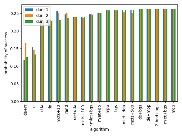
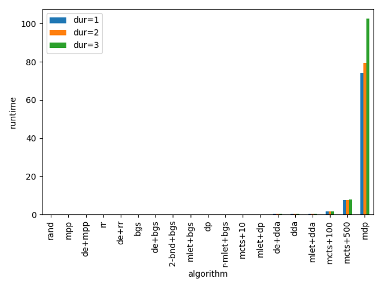
Figure 2: Bar plots for 2 processes.

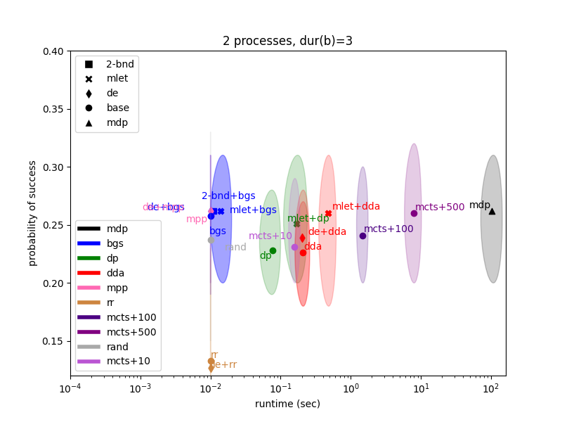
Figure 3: Average results for instances with 2 processes and $dur(b)=3$. Ellipse centers are averages over instances, the shaded area just covers the results for all 10 instances.

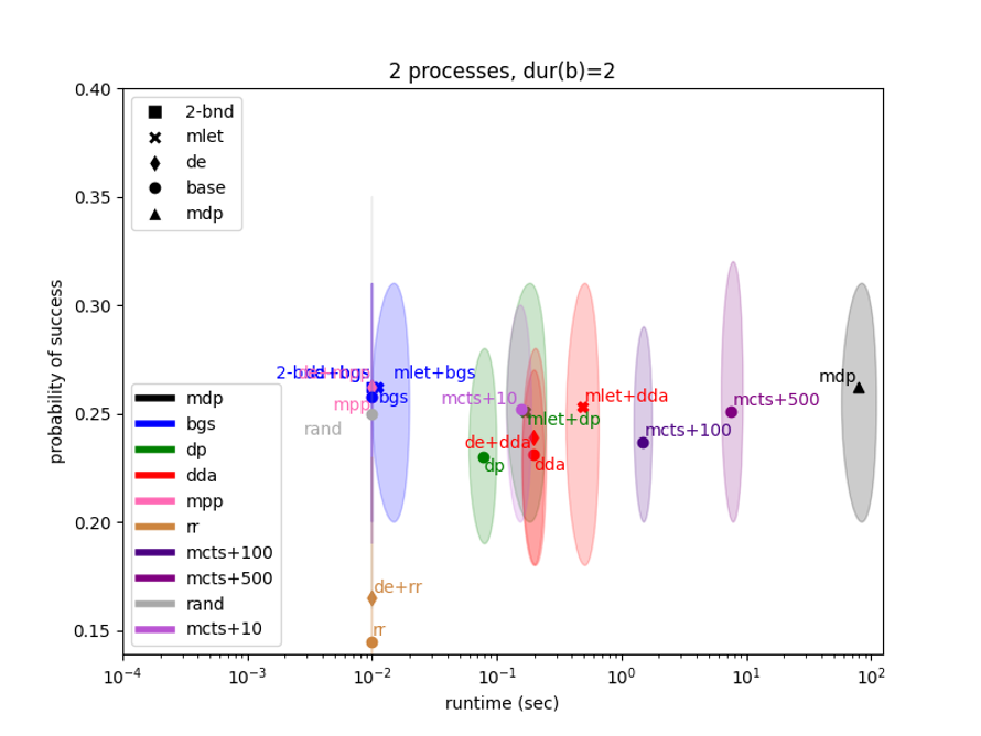
Figure 4: Average results for instances with 2 processes and $dur(b)=2$. Ellipse centers are averages over instances, the shaded area just covers the results for all 10 instances.

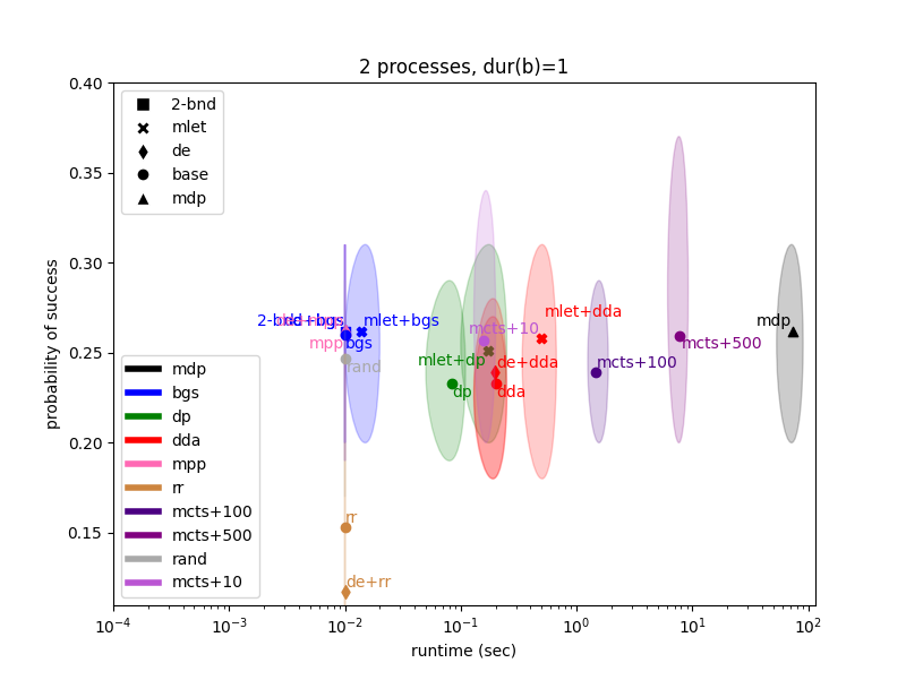
Figure 5: Average results for instances with 2 processes and $dur(b)=1$. Ellipse centers are averages over instances, the shaded area just covers the results for all 10 instances.

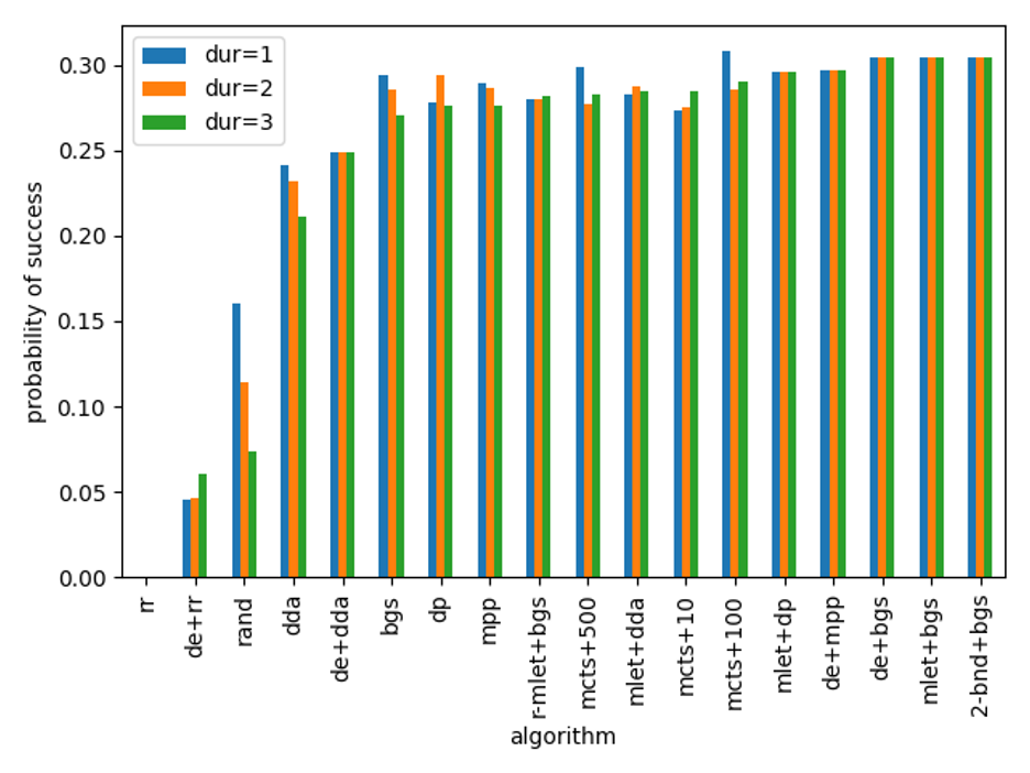
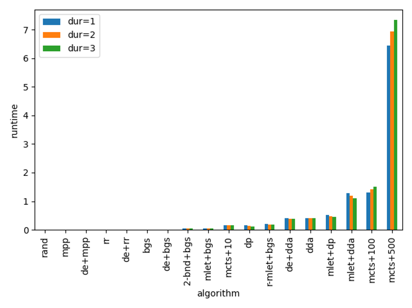
Figure 6: Bar plots for 5 processes.

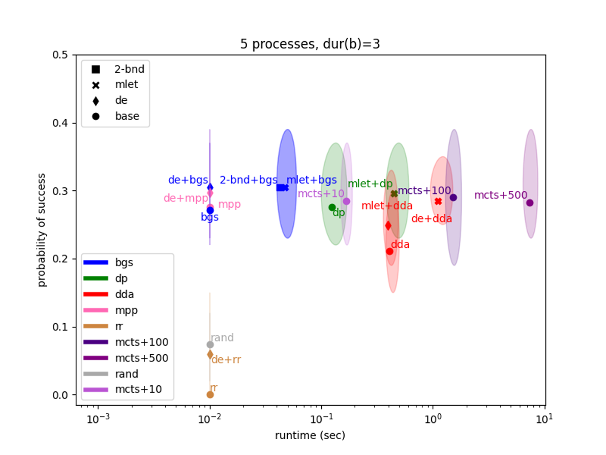
Figure 7: Average results for instances with 5 processes and $dur(b)=3$. Ellipse centers are averages over instances, the shaded area just covers the results for all 10 instances.

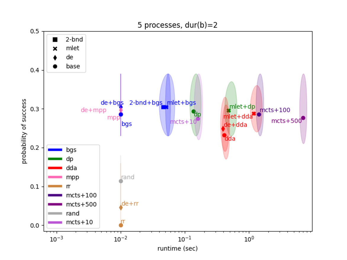
Figure 8: Average results for instances with 5 processes and $dur(b)=2$. Ellipse centers are averages over instances, the shaded area just covers the results for all 10 instances.

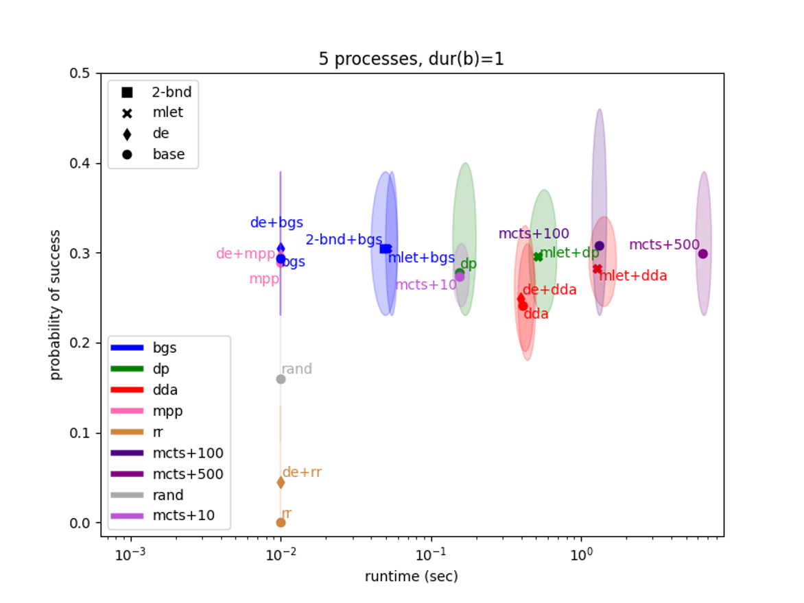
Figure 9: Average results for instances with 5 processes and $dur(b)=1$. Ellipse centers are averages over instances, the shaded area just covers the results for all 10 instances.

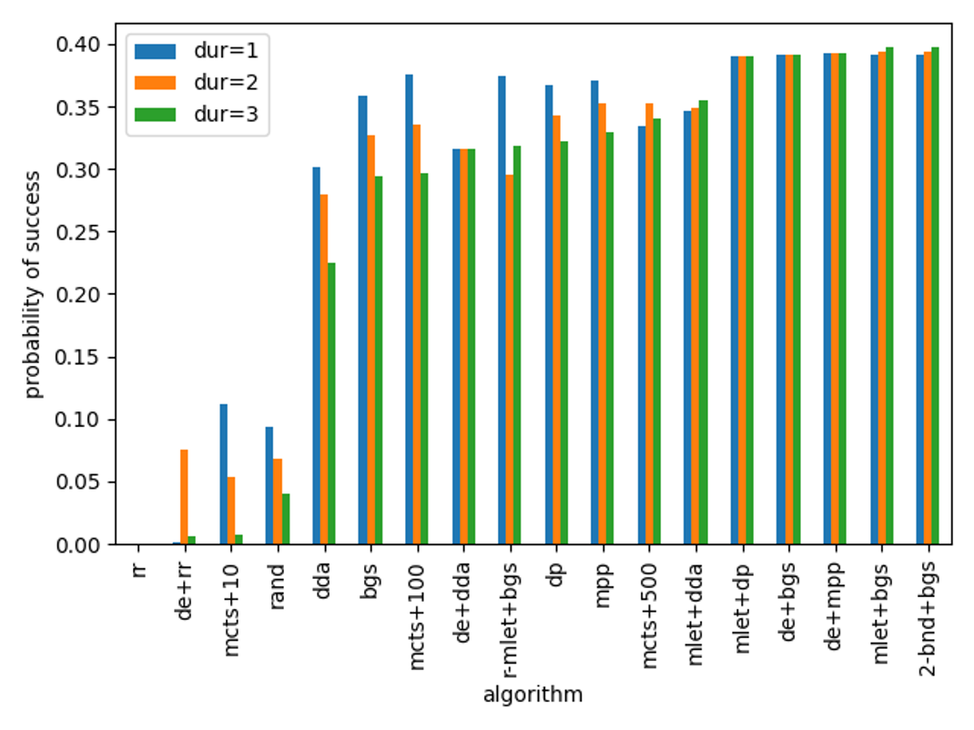
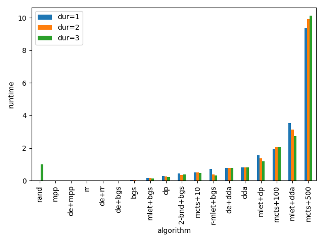
Figure 10: Bar plots for 10 processes.

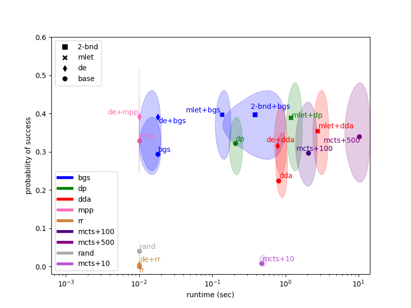
Figure 11: Average results for instances with 10 processes and $dur(b)=3$. Ellipse centers are averages over instances, the shaded area just covers the results for all 10 instances.

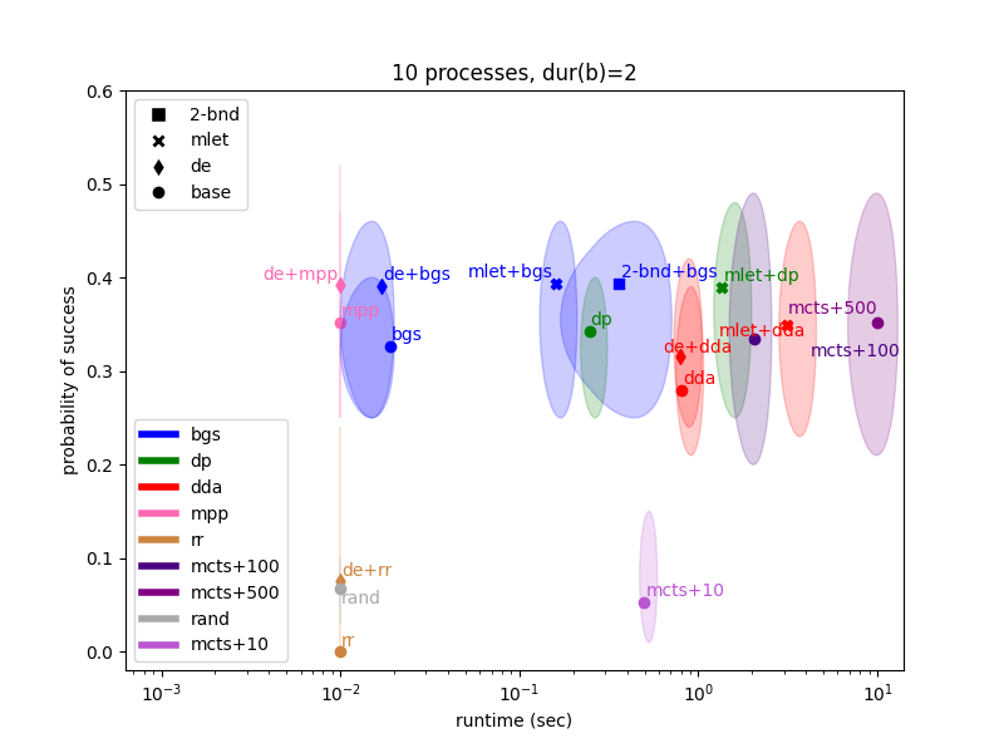
Figure 12: Average results for instances with 10 processes and $dur(b)=2$. Ellipse centers are averages over instances, the shaded area just covers the results for all 10 instances.

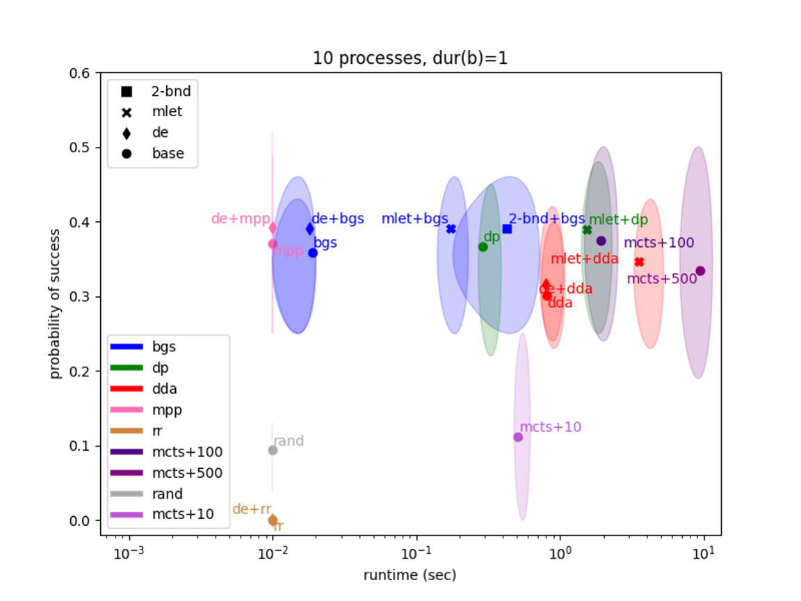
Figure 13: Average results for instances with 10 processes and $dur(b)=1$. Ellipse centers are averages over instances, the shaded area just covers the results for all 10 instances.

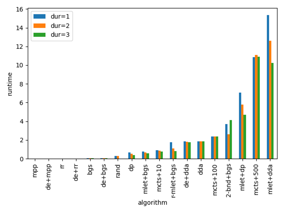
Figure 14: Bar plots for 20 processes. In both figures, the blue, orange and green bars represent the results for the instances where the base-level action durations are 1, 2 and 3, respectively. The left figure shows the average probability of success of each algorithm, and is sorted according to the green bars (because the time pressure is highest when the duration is 3). The right figure shows the average runtime of each algorithm, and is sorted according to the blue bars (for aesthetic reasons).

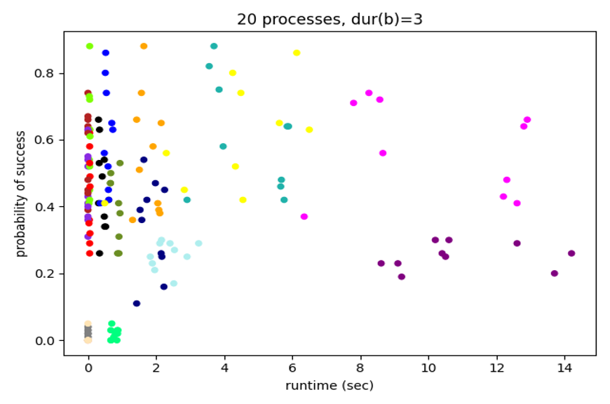
Figure 15: All figures present all the results (without averaging). The x-axis stands for the runtime and the y-axis stands for the empirical probability of success. The upper plots present the runtime in linear scale, and the lower plots in logarithmic scale. On the left the results are shown in their raw form, while on the right they are normalized (by the maximal values).

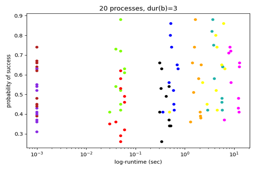
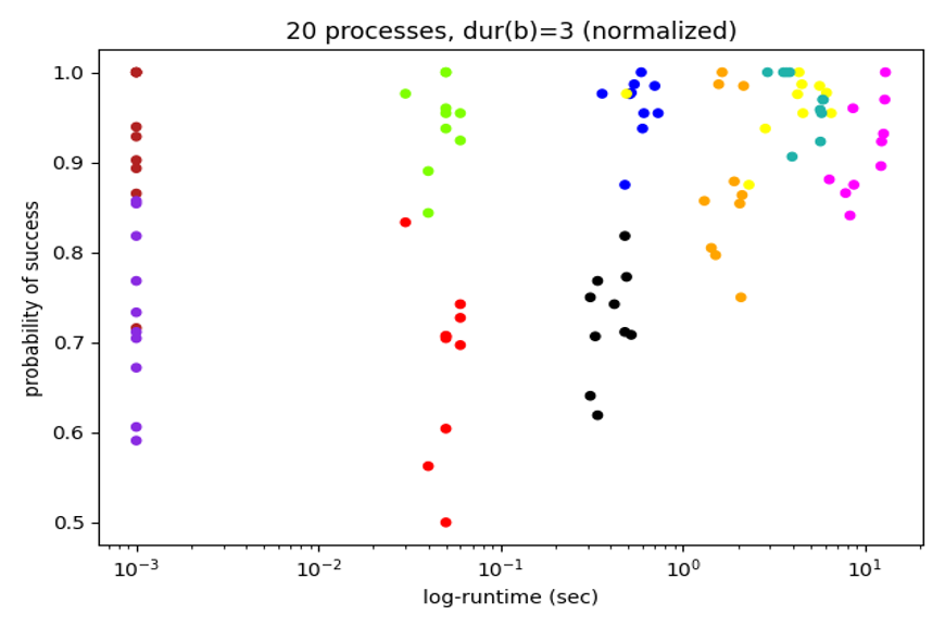
Figure 16: The figures present only the 10 algorithms with best probability of success. In both figures the runtime is in log-scale. On the right the results are normalized, and on the left they are not.

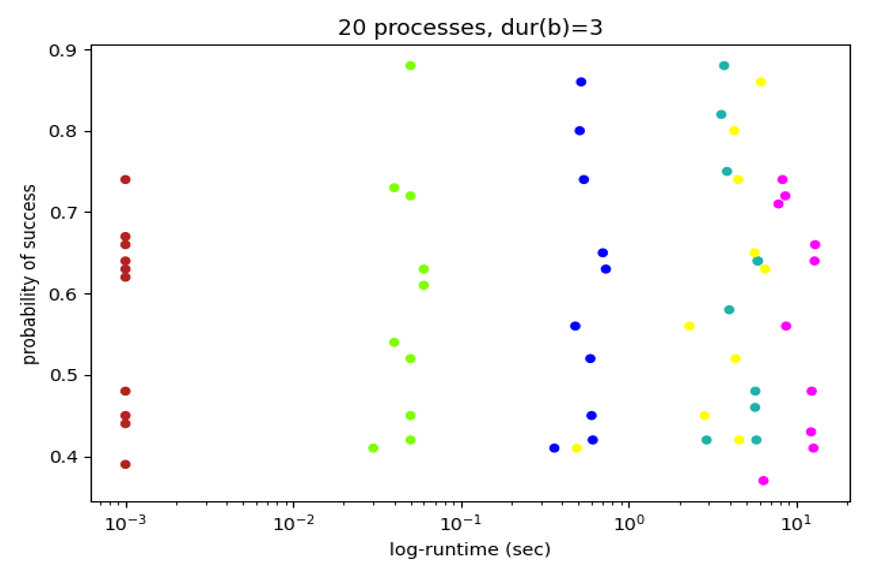
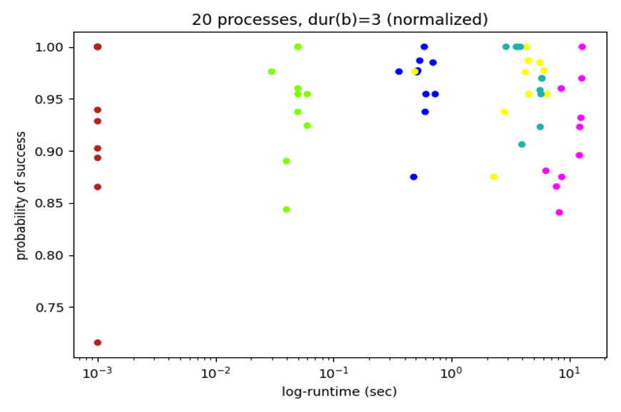
Figure 17: The figures present only the 6 algorithms with the best probability of success.

Figure 18: Average results for instances with 20 processes and $dur(b)=3$. Ellipse centers are averages over instances, the shaded area just covers the results for all 10 instances.

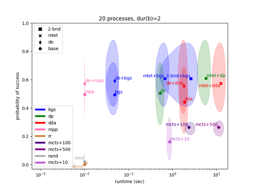
Figure 19: Average results for instances with 20 processes and $dur(b)=2$. Ellipse centers are averages over instances, the shaded area just covers the results for all 10 instances.

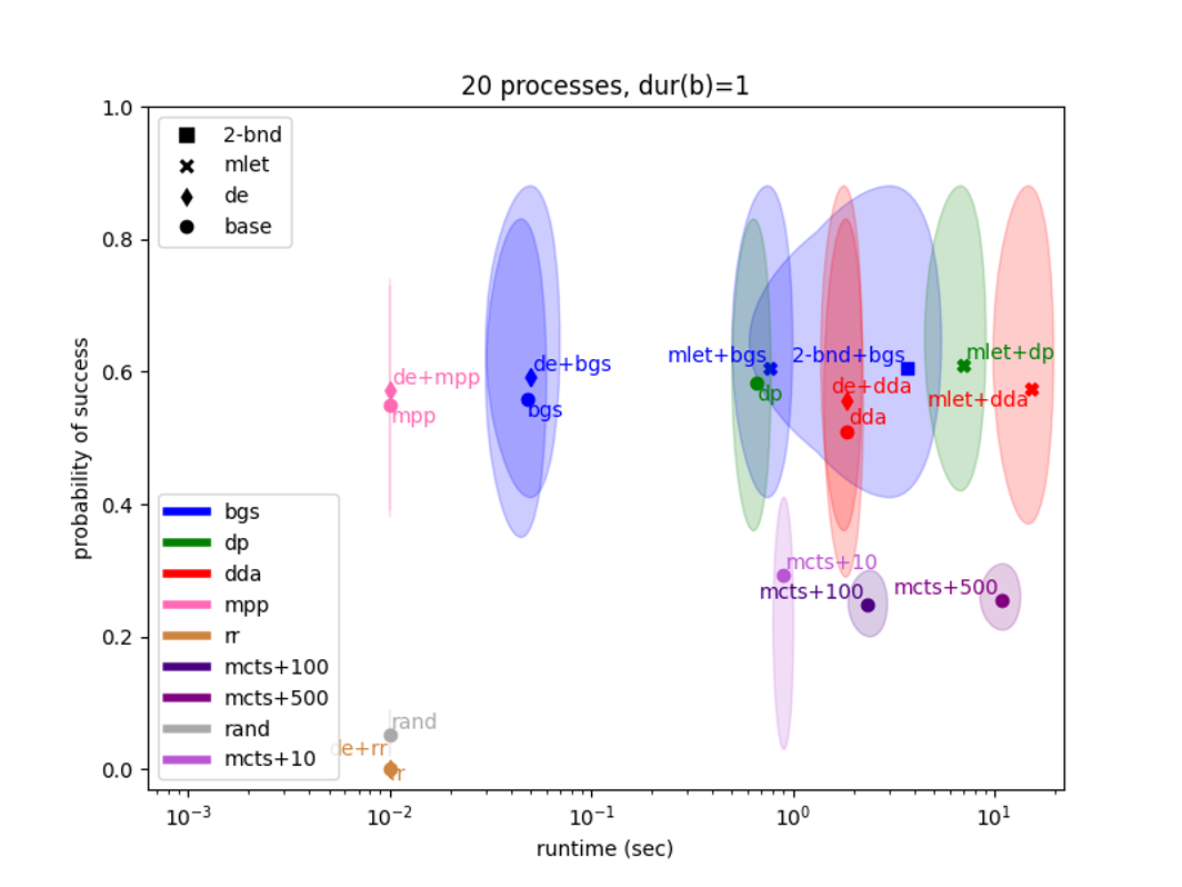
Figure 20: Average results for instances with 20 processes and $dur(b)=1$. Ellipse centers are averages over instances, the shaded area just covers the results for all 10 instances.

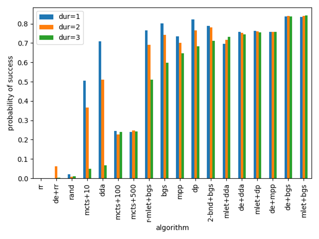
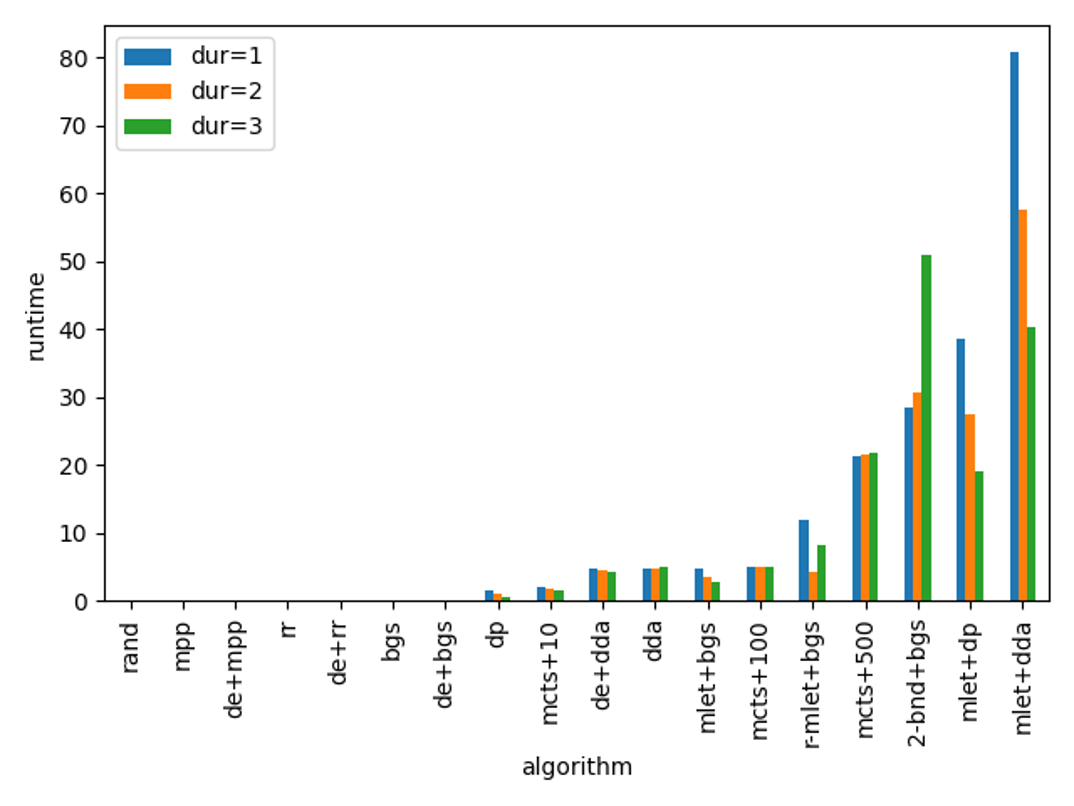
Figure 21: Bar plots for 50 processes.

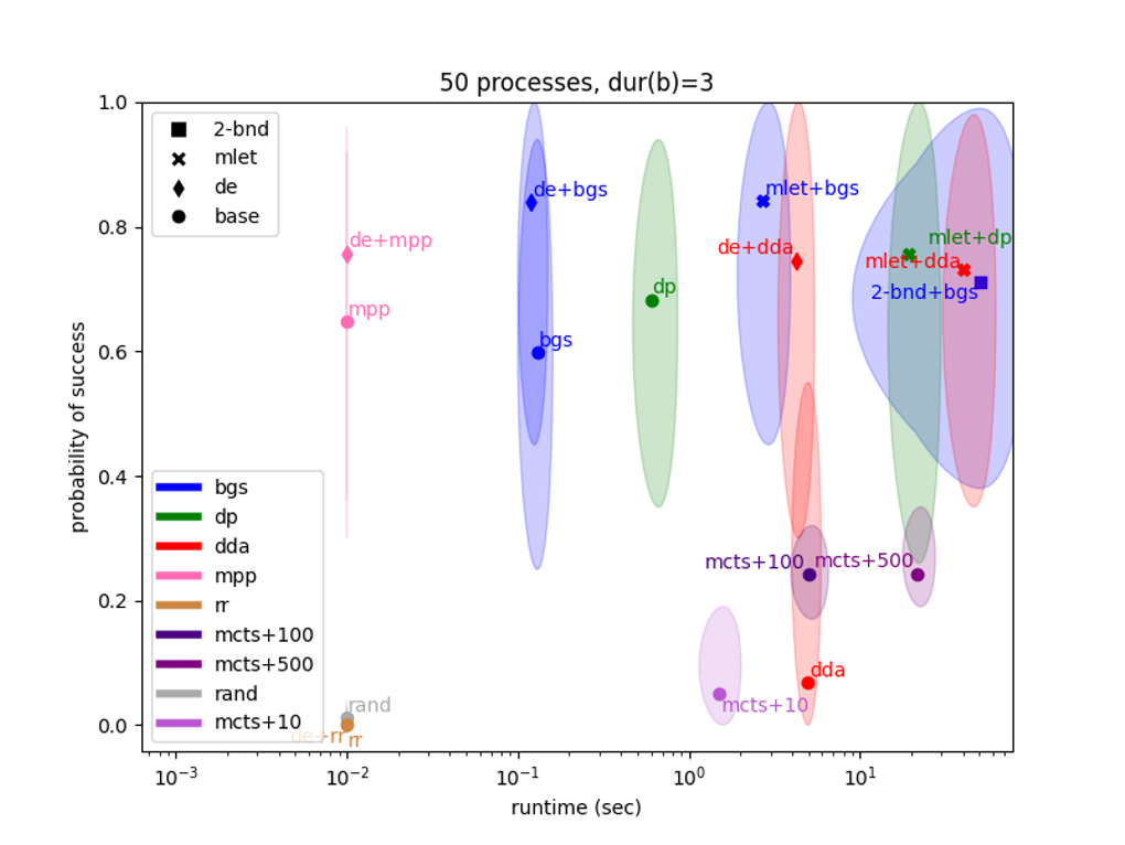
Figure 22: Average results for instances with 50 processes and $dur(b)=3$. Ellipse centers are averages over instances, the shaded area just covers the results for all 10 instances.

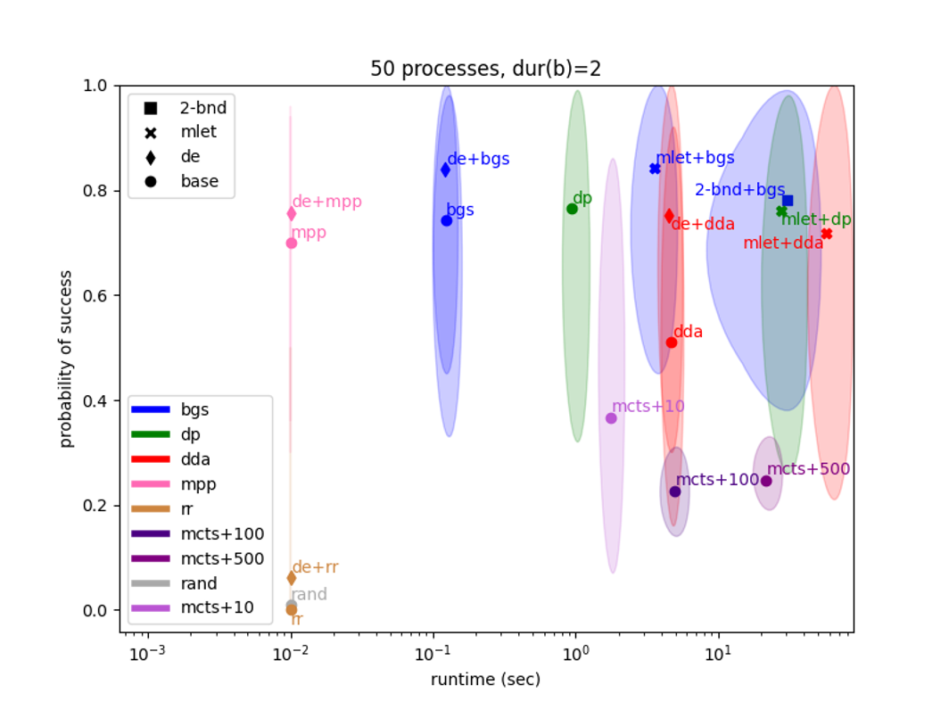
Figure 23: Average results for instances with 50 processes and $dur(b)=2$. Ellipse centers are averages over instances, the shaded area just covers the results for all 10 instances.

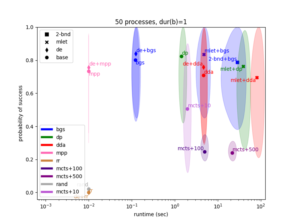
Figure 24: Average results for instances with 50 processes and $dur(b)=1$. Ellipse centers are averages over instances, the shaded area just covers the results for all 10 instances.

References

- Ambros-Ingerson, Steel et al. (1988) Ambros-Ingerson, J. A.; Steel, S.; et al. 1988. Integrating Planning, Execution and Monitoring. In Proceedings of AAAI, 21–26.
- Auer, Cesa-Bianchi, and Fischer (2002) Auer, P.; Cesa-Bianchi, N.; and Fischer, P. 2002. Finite-time analysis of the multiarmed bandit problem. Machine learning, 47(2): 235–256.
- Benton, Coles, and Coles (2012) Benton, J.; Coles, A. J.; and Coles, A. 2012. Temporal Planning with Preferences and Time-Dependent Continuous Costs. In Proceedings of ICAPS, 2–10.
- Browne et al. (2012) Browne, C. B.; Powley, E.; Whitehouse, D.; Lucas, S. M.; Cowling, P. I.; Rohlfshagen, P.; Tavener, S.; Perez, D.; Samothrakis, S.; and Colton, S. 2012. A survey of Monte-Carlo tree search methods. IEEE Transactions on Computational Intelligence and AI in Games, 4(1): 1–43.
- Cashmore et al. (2018) Cashmore, M.; Coles, A.; Cserna, B.; Karpas, E.; Magazzeni, D.; and Ruml, W. 2018. Temporal Planning While the Clock Ticks. In Proceedings of ICAPS, 39–46.
- Fikes, Hart, and Nilsson (1972) Fikes, R.; Hart, P. E.; and Nilsson, N. J. 1972. Learning and Executing Generalized Robot Plans. Artificial Intelligence, 3(1-3): 251–288.
- Haigh and Veloso (1998) Haigh, K. Z.; and Veloso, M. M. 1998. Interleaving planning and robot execution for asynchronous user requests. Autonomous Robots, 5: 79–95.
- Kocsis and Szepesvári (2006) Kocsis, L.; and Szepesvári, C. 2006. Bandit Based Monte-Carlo Planning. In Proceedings of ECML, volume 4212 of Lecture Notes in Computer Science, 282–293. Springer.
- Korf (1990) Korf, R. E. 1990. Real-Time Heuristic Search. Artif. Intell., 42(2-3): 189–211.
- Lemai and Ingrand (2004) Lemai, S.; and Ingrand, F. 2004. Interleaving temporal planning and execution in robotics domains. In Proceedings of AAAI, 617–622.
- Nourbakhsh (1997) Nourbakhsh, I. R. 1997. Interleaving planning and execution for autonomous robots. Springer Science & Business Media.
- Russell and Wefald (1991) Russell, S. J.; and Wefald, E. 1991. Principles of Metareasoning. Artificial Intelligence, 49(1-3): 361–395.
- Shperberg et al. (2019) Shperberg, S. S.; Coles, A.; Cserna, B.; Karpas, E.; Ruml, W.; and Shimony, S. E. 2019. Allocating Planning Effort When Actions Expire. In Proceedings of AAAI, 2371–2378.
- Shperberg et al. (2021) Shperberg, S. S.; Coles, A.; Karpas, E.; Ruml, W.; and Shimony, S. E. 2021. Situated Temporal Planning Using Deadline-aware Metareasoning. In Proceedings of ICAPS.
- Zilberstein and Russell (1996) Zilberstein, S.; and Russell, S. J. 1996. Optimal Composition of Real-Time Systems. Artificial Intelligence, 82(1-2): 181–213.