Expectation consistency for calibration of neural networks

Abstract

Despite their incredible performance, it is well reported that deep neural networks tend to be overoptimistic about their prediction confidence. Finding effective and efficient calibration methods for neural networks is therefore an important endeavour towards better uncertainty quantification in deep learning. In this manuscript, we introduce a novel calibration technique named expectation consistency (EC), consisting of a post-training rescaling of the last layer weights by enforcing that the average validation confidence coincides with the average proportion of correct labels. First, we show that the EC method achieves similar calibration performance to temperature scaling (TS) across different neural network architectures and data sets, all while requiring similar validation samples and computational resources. However, we argue that EC provides a principled method grounded on a Bayesian optimality principle known as the Nishimori identity. Next, we provide an asymptotic characterization of both TS and EC in a synthetic setting and show that their performance crucially depends on the target function. In particular, we discuss examples where EC significantly outperforms TS.

1 Introduction

As deep learning models become more widely employed in all aspects of human society, there is an increasing necessity to develop reliable methods to properly assess the trustworthiness of their predictions. Indeed, different uncertainty quantification procedures have been proposed to measure the confidence associated with trained neural network predictions [Abdar et al., 2021, Gawlikowski et al., 2021]. Despite their popularity in practice, it is well known that some of these metrics, such as interpreting the last-layer softmax scores as confidence scores, lead to an overestimation of the true class probability [Guo et al., 2017]. As a consequence, various methods have been proposed to calibrate neural networks [Gal and Ghahramani, 2016, Guo et al., 2017, Maddox et al., 2019, Minderer et al., 2021].

In this work, we propose a novel method for the post-training calibration of neural networks named expectation consistency (EC). It consists of fixing the scale of the last-layer weights by enforcing the average confidence to coincide with the average classification accuracy on the validation set. This procedure is inspired by optimality conditions steaming from the Bayesian inference literature. Therefore, it provides a mathematically principled alternative to similar calibration techniques such as temperature scaling, besides being simple to implement and computationally efficient. Our goal in this work is to introduce the expectation consistency calibration method, illustrate its performance across different deep learning tasks and provide theoretical guarantees in a controlled setting. More specifically, our main contributions are:

• We introduce a novel method, Expectation Consistency (EC) to calibrate the post-training predictions of neural networks. The method is based on rescaling the last-layer weights so that the average confidence matches the average accuracy on the validation set. We provide a Bayesian inference perspective on expectation consistency that grounds it mathematically.

• While calibration methods abound in the uncertainty quantification literature, we compare EC to a close and widely employed method in the deep learning practice: temperature scaling (TS). Our experiments with different network architectures and real data sets show that the two methods yield very similar results in practice.

• We provide a theoretical analysis of EC in a high-dimensional logistic regression exhibiting overconfidence issues akin to deep neural networks. We show that in this setting EC consistently outperforms temperature scaling in different uncertainty metrics. The theoretical analysis also elucidates the origin of the similarities between the two methods.

The manuscript is structured as follows : after a review of the literature and an exposition of the EC method (Section 3), we compare the performance of EC with TS on real data (Section 4) and show that the two methods behave similarly. In complement to Section 4, we provide in Section 5 a theoretical analysis of both methods and describe a synthetic setting in which EC outperforms TS.

The code used in this project is available at the repository https://github.com/SPOC-group/expectation-consistency

  Input: Validation set $(\vec{x}_{i},y_{i})_{i=1}^{n_{val}}$, classifier $\hat{f}:\mathcal{X}\to\mathbb{R}^{K}$

  Compute the logits $\bm{z}_{i}=\hat{f}(\bm{x}_{i})\in\mathbb{R}^{K}$ and output $\hat{y}_{i}=\arg\max_{k}{\vec{z}_{i}}_{k}$

  Compute the accuracy on validation set $\mathcal{A}_{val}=\frac{1}{n_{val}}\sum_{i}\delta(y_{i}=\hat{y}_{i})$

  Determine $T_{EC}$ such that $\frac{1}{n_{val}}\sum_{i}\max_{k}\sigma^{(k)}(\nicefrac{{\vec{z}_{i}}}{{T}})=\mathcal{A}_{val}$

  Output: Temperature $T_{\rm EC}$, and probabilities on new samples $\max_{k}\sigma^{(k)}(\nicefrac{{\vec{z}^{\rm new}}}{{T_{\rm EC}}})$,

Algorithm 1 Expectation consistency (EC)

1.1 Related work

Calibration of neural networks —

The calibration of predictive models, in particular neural networks, has been extensively studied, see Abdar et al. [2021], Gawlikowski et al. [2021] for two reviews. In particular, modern neural network architectures have been observed to return overconfident predictions [Guo et al., 2017, Minderer et al., 2021]. While their overconfidence could be partly attributed to their over-parametrization, some theoretical works [Bai et al., 2021, Clarté et al., 2022b, a] have shown that even simple regression models in the under-parametrized regime can exhibit overconfidence.

There exists a range of methods that guarantee calibration asymptotically (i.e. when the number of samples is sufficiently large) without assuming anything about the data distribution, see e.g. Gupta et al. [2020]. However, for a limited number of samples, it is less clear which of the proposed methods provides the most accurate calibration.

Temperature scaling —

Guo et al. [2017] proposed Temperature Scaling (TS), a simple post-processing method consisting of rescaling & cross-validating the norm of the last-layer weights. Due to its simplicity and efficiency compared to other methods such as Platt scaling [Platt, 2000] or histogram binning [Zadrozny and Elkan, 2001], TS is widely used in practice to calibrate the output of neural networks [Abdar et al., 2021]. Moreover, Clarté et al. [2022a] has shown that in some settings, TS is competitive with much more costly Bayesian approaches in terms of uncertainty quantification. While Gupta et al. [2020] has shown that without any assumption on the data model, injective calibration methods such as TS cannot be calibrated in general, Guo et al. [2017] conclude that: ”Temperature scaling is the simplest, fastest, and most straightforward of the methods, and surprisingly is often the most effective.” This justifies why TS is used so widely in practice.

Bayesian methods —

Bayesian methods such as Gaussian processes allow estimating the uncertainty out of the box for a limited number of samples under (at least implicit) data distribution assumptions. When the data-generating process is known, the best way to estimate the uncertainty of a model is to use the predictive posterior. However, Bayesian inference is often intractable, and several approximate Bayesian methods have been adapted to neural networks, such as deep ensembles [Lakshminarayanan et al., 2017a] or weight averaging [Maddox et al., 2019]. On the other hand, the strength of posthoc methods like temperature scaling is that it applies directly to the unnormalized output of the network, and does not require additional training. A comparable Bayesian approach has been developed in Kristiadi et al. [2020], where a Gaussian distribution is applied to the last-layer weights. Bayesian methods typically involve sampling from a high-dimensional posterior [Mattei, 2019], and different methods have been proposed to compute them efficiently [Graves, 2011, Gal and Ghahramani, 2016, Lakshminarayanan et al., 2017b, Maddox et al., 2019].

Notation —

We denote $[n]\coloneqq\{1,\cdots,n\}$; $\bm{1}(A)$ the indicator function of the set $A$; $\mathcal{N}(\bm{x}|\mu,\Sigma)$ the multi-variate Gaussian p.d.f. with mean $\mu$ and covariance $\Sigma$.

2 Setting

Consider a $K$-class classification problem where a neural network classifier is trained on a data set $(\vec{x}_{i},y_{i})_{i\in[n]}\in\mathbb{R}^{d}\times[K]$. Without loss of generality, for a given input $\bm{x}\in\mathbb{R}^{d}$ we can write the output of the classifier as a $K$-dimensional vector $\bm{z}(\bm{x})=W\bm{\varphi}(\bm{x})\in\mathbb{R}^{K}$, where we have denoted the last-layer features by $\bm{\varphi}:\mathbb{R}^{d}\to\mathbb{R}^{p}$ and the read-out weights $W\in\mathbb{R}^{K\times p}$. We define the confidence of the prediction for class $k$ as:

$$\hat{f}(\vec{x},k)\coloneqq\sigma^{(k)}(\bm{z}(\bm{x}))=\frac{e^{z_{k}(\bm{x})}}{\sum\limits_{l\in[K]}e^{z_{l}(\bm{x})}}\in(0,1)$$ (1)

where $\sigma:\mathbb{R}^{K}\to(0,1)^{K}$ is the softmax activation function. In short, $\hat{f}(\vec{x},k)$ defines a probability, as estimated by the network, that $\vec{x}$ belongs to class $k$. For a given $\bm{x}\in\mathbb{R}^{d}$, the final prediction of the model is then given by $\hat{y}(\vec{x})=\arg\max_{k}\hat{f}(\vec{x},k)\in[K]$, and the associated prediction confidence $\hat{f}(\vec{x})=\max_{k}\hat{f}(\vec{x},k)=\hat{f}(\bm{x},\hat{y}(\bm{x}))\in(0,1)$. As it is common practice, in what follows we will be mostly interested in the case in which the network is trained by minimizing the empirical risk (ERM) with the cross-entropy loss:

$$\quad\ell(\hat{f}(\vec{x}),y) =-\log\hat{f}(\vec{x},y)$$

$$=\sum_{k=1}^{K}\delta(y=k)\log\sigma^{(k)}(W\bm{\phi}(\vec{x})),$$

although many of the concepts introduced here straightforwardly generalize to other training procedures. The quality of the training is typically assessed by the capacity of the model to generalize on unseen data. This can be quantified by the test misclassification error and the test loss:

$$\mathcal{E}_{g}=\mathbb{E}_{\vec{x},y}\left[\delta\left(\hat{y}(\vec{x})\neq y\right)\right],\quad\mathcal{L}_{g}=-\mathbb{E}_{\vec{x},y}\left[\log\hat{f}(\vec{x},y)\right]$$

These are point performance measures. However, often we are also interested in quantifying the quality of the network prediction confidence. Different uncertainty metrics exist in the literature, but some of the most current ones are the calibration, expected calibration error (ECE) and Brier score (BS), defined as:

$$\begin{cases}\Delta_{p}&=p-\mathbb{P}_{\vec{x},y}\left(\hat{y}(\bm{x})=y|\hat{f}(\vec{x})=p\right)\\ \text{ECE}&=\mathbb{E}_{\vec{x},y}\left(|\Delta_{\hat{f}(\vec{x})}|\right)\\ BS&=\mathbb{E}_{\vec{x},y}\left(\sum_{k=1}^{K}(\hat{f}(\vec{x},k)-\delta(y=k))^{2}\right)\end{cases}$$ (2)

Note that the Brier score is a proper loss, meaning that it is minimized when $\hat{f}(\vec{x},k)$ is the true marginal distribution $\mathbb{P}(y=k|\bm{x})$. This is not the case of the ECE: indeed, the estimator defined as $\hat{f}(\vec{x},k)=\mathbb{P}(y=k)$ has $0$ ECE but does not correspond to the marginal distribution of $y$ conditioned on $\vec{x}$ and has suboptimal test error. Finally, we introduce the confidence function with temperature $T>0$:

$$\hat{f}_{T}(\vec{x},k)=\sigma^{(k)}(\nicefrac{{W\varphi(\vec{x})}}{{T}}).$$ (3)

Dataset	Model	$\mathcal{E}_{g}$	$T_{TS}$	$T_{EC}$	$ECE$	$ECE_{TS}$	$ECE_{EC}$	$BS$	$BS_{TS}$	$BS_{EC}$
SVHN	Resnet20	6.8 %	1.59	1.55	2.6 %	1.5 %	1.3 %	10.5 %	10.4 %	10.4 %
CIFAR10	Resnet20	13.5 %	1.37	1.38	5.3 %	1.9 %	1.9 %	20.0 %	19.43%	19.2 %
CIFAR10	Resnet56	13.1 %	1.42	1.43	6.0%	2.5 %	2.4 %	20.2 %	19.3 %	19.3 %
CIFAR10	Densenet121	12.5 %	1.78	1.86	7.9 %	3.0 %	2.5 %	20.4 %	18.6 %	18.5 %
CIFAR100	Resnet20	31.0 %	1.44	1.44	10.2 %	1.7 %	1.7 %	44.3 %	42.5 %	42.5 %
CIFAR100	Resnet56	27.3 %	1.73	1.79	14 %	2.6 %	2.2 %	41 %	38.0 %	38.0 %
CIFAR100	VGG19	26.4 %	2.14	2.28	19.9 %	5.3 %	4.8 %	44.8 %	37.2 %	36.9 %
CIFAR100	RepVGG-A2	22.5 %	1.07	1.16	5.3 %	4.6 %	4.4 %	32.1 %	31.9 %	32.0 %

Figure 1: Comparison of expected calibration error (ECE) and Brier score (BS) of temperature scaling (TS) and expectation consistency (EC) on various models and data sets. We see very minor differences between the two calibration methods. Given how well TS works in practice we conjecture at least the same for EC.

3 Expectation consistency Calibration

The method proposed in this work acts similarly as the temperature scaling method Guo et al. [2017] discussed in the related work section, with a key difference in how the temperature parameter is chosen. The popular and widely adopted temperature scaling (TS) procedure will also serve as the main benchmark in what follows.

Temperature scaling —

Although the score-based confidence measure introduced in (1) might appear natural, numerical evidence suggests that for modern neural network architectures, it tends to be overconfident [Guo et al., 2017]. In other words, it overestimates the probability of class belonging. To mitigate overconfidence, Guo et al. [2017] has introduced a post-training calibration method known as temperature scaling (TS) [Minderer et al., 2021, Wang et al., 2021]. Temperature scaling consists of rescaling the trained network output $\bm{z}\mapsto\nicefrac{{\bm{z}}}{{T}}$ by a positive constant $T>0$ (the ”temperature”) which is then be tuned to adjust the prediction confidence. Equivalently, TS can be seen as a re-scaling of the norm of the last-layer weights $W$. Guo et al. [2017] has found that choosing $T$ that minimizes the cross-entropy loss on the validation set $\{(\vec{x}_{i},y_{i})_{i\in[n_{val}]}$:

$$T_{\rm TS}=\arg\min_{T>0}\left(-\sum_{i=1}^{n_{val}}\ell(\hat{f}_{T}(\vec{x}_{i},y_{i}))\right)$$ (4)

results in a better calibrated rescaled predictor $\hat{f}_{T_{\rm TS}}$. To get a feeling for its effect on the confidence, it is instructive to look at the two extreme limits of TS. On one hand, if $T\ll 1$, the softmax will be dominated by the class with the largest confidence, eventually converging to a hard-thresholding $T\rightarrow 0^{+}$. This will typically lead to an overconfident predictor. On the other hand, for $T\gg 1$, the softmax will be less and less sensitive to the trained weights, converging to a uniform vector at $T\to\infty$. This will typically correspond to an underconfident predictor. Therefore, by tuning $T$, we can either make a predictor less overconfident (by lowering the temperature $T<1$) or less underconfident (by increasing the temperature $T>1$).

Temperature scaling is a specific instance of matrix/vector scaling, where the logits $z_{i}$ are multiplied by a matrix/vector before the softmax. Despite being more general, matrix and vector scaling have been observed in Guo et al. [2017] to perform worse than TS. Different variants of TS have been developed. Similarly to vector scaling, class-based temperature scaling [Frenkel and Goldberger, 2021] computes one temperature per class and finds the best temperature by minimizing the validation ECE instead of the validation loss. While TS can be naturally applied to the last-layer output of neural networks, Kull et al. [2019] has extended TS to more general multi-class classification models.

Expectation consistency —

In this work, we introduce a novel calibration method, which we will refer to as Expectation Consistency (EC). As for TS, the starting point is a pre-trained confidence function $\hat{f}$ which we rescale $\hat{f}_{T}$ by introducing a temperature $T>0$. The key difference resides in the procedure we use to tune the temperature. Instead of minimizing the validation loss (4), we search for a temperature such that the average confidence is equal to the proportion of correct labels in the test set. In mathematical terms, we define $T_{\rm EC}$ such that the following is satisfied:

$$\frac{1}{n_{\rm val}}\sum_{i=1}^{n_{\rm val}}\hat{f}_{T_{\rm EC}}(\vec{x}_{i})=\frac{1}{n_{\rm val}}\sum_{i=1}^{n_{\rm val}}\bm{1}(\hat{y}(\vec{x}_{i})=y_{i})$$ (5)

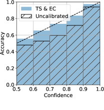
Figure 2: Left: The validation loss and average confidence of the model, as a function of the temperature $T$, model is DenseNet121 trained on CIFAR10. The dark dashed line is the accuracy for the validation set. Orange (respectively blue) cross corresponds to $T_{EC}$, $T_{TS}$. Middle: ECE of the model as a function of $T$, blue and orange dots respectively correspond to TS and EC. Right: Reliability diagram of Resnet20 trained on CIFAR10, before and after Temperature scaling. The reliability diagram after EC is indistinguishable from the one of TS.

The intuition behind this choice is the following: a calibrated classifier is such that for all $p\in(0,1),\Delta_{p}=0$. This condition is not achievable by tuning the temperature parameter $T$, so a less strict condition is to enforce it in expectation $\mathbb{E}_{\bm{x}}\left[\Delta_{\hat{f}(\bm{x})}\right]=0$, ensuring that the classifier is calibrated on average. This is equivalent to enforcing the average confidence to be equal to the probability of predicting the correct class on a validation set. Note that the fact that we directly compare to the confidence on the validation set is analogous to what is done in the conformal prediction [Papadopoulos et al., 2002] methods to estimate prediction sets (as opposed to calibration that we are aiming at here).

It is instructive to consider a Bayesian perspective on EC. For the sake of this paragraph, assume that both the training and validation data were independently drawn from a parametric probability distribution $p(\bm{x},y|\theta)$. If we had access to the distribution of the data (but not the specific realization of the parameters $\theta$), the Bayes-optimal confidence function would be given by the expectation of $f_{\star}(\bm{x}|\theta)=p(y|\bm{x},\theta)$ with respect to the posterior distribution of the weights given the training data $p(\theta|(\bm{x}_{i},y_{i})_{i\in[n]})$. In this case, one would not even need a validation set since the expected test accuracy would be predicted by the uncertainties under the posterior. In Section 5.1 we illustrate this discussion for concrete data distribution. This expectation consistency property of the Bayes-optimal predictor is known as the Nishimori condition in the information theory and statistical physics literature [Iba, 1999, Méasson et al., 2009, Zdeborová and Krzakala, 2016]. Therefore, from this perspective requesting condition (5) to hold can be seen as enforcing the Nishimori conditions for the rescaled confidence function. The Nishimori conditions are also used within the expectation-maximization algorithm for learning hyperparameters Dempster et al. [1977]. We describe in Section 5 how to interpret both temperature scaling and expectation consistency as learning procedures for the hyperparameter $T$. The main idea behind the EC method proposed here is that even in the absence of knowledge of the data-generating model, the expectation consistency (5) relation should hold for a calibrated uncertainty quantification method.

Note that $T_{EC}$ exists and is unique. Indeed, the average confidence is a decreasing function of the temperature, converging to one when $T\to 0^{+}$ and to zero when $T\to\infty$. Therefore, there is a unique $T_{EC}$ that satisfies the constraint (5), and in practice, it can be found by bisection. We refer to Figure 2 for an illustration of the uniqueness of $T_{EC}$. Moreover, note that expectation consistency is more flexible than temperature scaling: in multi-class classification problems, we can fix the temperature so that the average confidence is equal to the top $N$ accuracy for any $N\in[K]$. In this work, we focus on the top $1$ accuracy.

4 Experiments on real data

Figure 3: Left: Accuracy of Resnet20 model (Left), the temperature returned by TS and EC (Middle) and ECE of the model (Right) as a function of the size of the training set $\alpha=\nicefrac{{n_{\rm train}}}{{50000}}$. The model is trained with the same hyperparameters as in Figure 1. Again we see that the two methods are comparable even at largely different sample sizes.

.

In this section, we present numerical experiments carried out on real data sets and compare the performance of EC and TS. As we will see, both methods yield similar calibration performances in practical scenarios.

Experimental setup —

We consider the performance of the calibration methods from Section 3 in image classification tasks. Experiments were conducted on three popular image classification data sets:

• SVHN Netzer et al. [2011] is made of colored $32\times 32$ labelled digit images. Train/validation/test set sizes are 65931/7325/26032.

• CIFAR10 and CIFAR100 data sets Krizhevsky [2009], consisting of $32\times 32$ colored images from 10/100 classes (dog, cat, plane, etc.), respectively. Train/validation/test sets sizes are 45000/5000/10000 images for CIFAR10, 50000/5000/5000 for CIFAR100.

We consider different neural network architectures adapted to image classification tasks: ResNets [He et al., 2016], DenseNets [Huang et al., 2017], VGG [Simonyan and Zisserman, 2014] and RepVGG [Ding et al., 2021]. For CIFAR100, pre-trained models available online were employed. More details on the training procedure are available in Appendix A.

Results —

We refer to Table 1 for a comparison of TS and EC on the various data sets and models discussed above. Curiously, we observe that both EC and TS yield very similar temperatures across the different tasks and architectures, implying a similar ECE and Brier score. In particular, note that both methods give $T>1$, consistent with the fact that the original networks were overconfident. Therefore, as expected, both methods improve the calibration of the classifiers.

The right panel of Figure 2 shows the reliability diagram of the ResNet 20 trained on CIFAR10: we observe that before applying TS and EC, the accuracy is lower than the confidence. In other words, the model is overconfident and both TS and EC improve the calibration of the model.

Note that both methods improve the Brier score and yield very similar results. From the computational cost perspective, EC is as efficient to run as TS, and requires only a few lines of code, see the GitHub repository where we provide the code to reproduce the experiments discussed here. However, we believe expectation consistency is a more principled calibration method, as it constrains the confidence of the model to correspond to the accuracy and has a natural Bayesian interpretation. Moreover, as we will discuss in Section 5, we can derive explicit theoretical results for EC.

Our experiments suggest that the similarity between TS and EC is independent of the accuracy of the model. Indeed, in Figure 3, we observe the accuracy and ECE of a ResNet model trained on different amounts of data. As expected, the accuracy of the model increases with the amount of training data. We observe in the middle and right panels that the temperatures and ECE obtained from both methods are extremely similar, independently of the accuracy of the model. Finally, we plot in the middle panel of Figure 2 the ECE as a function of the temperature and observe that neither $T_{TS}$ nor $T_{EC}$ is close to the minimum of ECE. However, as we have discussed in Section 3, ECE is only one uncertainty quantification metric and is not a proper loss, so we wish not to optimize the temperature for this metric in particular.

Experiments on corrupted data —

In Appendix C we compare the performance of EC and TS on an image classification task where the test data is corrupted. We use the same datasets and architectures as in Section 4, but for some image classes, the target labels on the test data are randomly chosen. The goal of introducing a class-dependent noise is to evaluate both methods in a more realistic scenario where there is a distribution shift between the training and test data, as done in hendrycks_benchmarking_2019. We report in Table 1 of the Appendix the performance of EC and TS in terms of ECE and Brier score. We observe that EC yields an reduction of the test ECE of 7 % on average, showing that EC is a competitive alternative to TS in more realistic scenarios. Note that in this setting, EC and TS yield different temperatures, contrary to the results described in Table 1. The full experimental details are described in Appendix C.

5 Theoretical analysis of the EC

As we have seen in Section 4, our experiments with real data and neural network models suggest that despite their different nature, EC and TS achieve a similar calibration performance across different architectures and data sets. In this section, we investigate EC and TS in specific settings where we can derive theoretical guarantees on their calibration properties.

Figure 4: ECE of regularized logistic regression with three different values of $\lambda$ ($10^{-4},\lambda_{\rm error},\lambda_{\rm loss}$): uncalibrated, after temperature scaling, and after expectation consistency. From left to right: $\sigma_{\star}=\sigma_{{\rm logit}},\sigma_{{\rm affine}},\sigma_{{\rm constant}}$ respectively.

For concreteness, in the examples that follow we will focus on binary classification problems for which, without loss of generality, we can assume $y\in\{-1,+1\}$. In this encoding, the softmax function is equivalent to the logit $\sigma(t)\coloneqq(1+e^{-t})^{-1}$, and the hard-max is given by the sign function. Further, we assume that both the training $(\bm{x}_{i},y_{i})_{i\in[n]}$ and validation set $(\bm{x}_{i},y_{i})_{i\in[n_{val}]}$ were independently drawn from the following data generative model:

$$f_{\star}(\bm{x}) \coloneqq\mathbb{P}(y^{\mu}=1|\bm{x}^{\mu})=\sigma_{\star}\left(\frac{\bm{w}_{*}^{\top}\bm{x}^{\mu}}{T_{\star}}\right)$$

$$\bm{x}^{\mu} \sim\mathcal{N}(\bm{0},\nicefrac{{1}}{{d}}\mathbf{I}_{d}),\quad\bm{w}_{*}\sim\mathcal{N}(\bm{0},\mathbf{I}_{d})$$ (6)

with $\sigma_{\star}:\mathbb{R}\to(0,1)$ an activation function and $T_{*}>0$ explicitly parametrizing the norm of the weights.

First, in Section 5.1 we provide a Bayesian interpretation of both the TS and EC methods, in an example where $T_{\rm{TS}}=T_{\rm{EC}}=T_{\star}$. Next, in Section 5.2 we analyze a misspecified empirical risk minimization setting where they yield different results. Finally, we discuss in Section 5.3 one case in which EC consistently outperforms TS.

5.1 Relation with Bayesian estimation

Consider a Bayesian inference problem: given the training data $\mathcal{D}\coloneqq\{(\bm{x}_{i},y_{i})_{i\in[n]}\}$, what is the predictor that maximizes the accuracy? If the statistician had complete access to the data generating process (5), this would be given by integrating the likelihood of the data over the posterior distribution of the weights given the data:

$$f_{\rm{bo}}(\bm{x})\coloneqq\mathbb{P}(y=1|\mathcal{D},\bm{x})=\int{\rm d}\bm{w}\leavevmode\nobreak\ \sigma\left(\frac{\bm{w}^{\top}\bm{x}}{T_{*}}\right)p(\bm{w}|\mathcal{D},T_{\star})$$

where the posterior distribution is explicitly given by:

$$p(\bm{w}|\mathcal{D},T_{\star})\propto\mathcal{N}(\bm{w}|0,\mathbf{I}_{d})\prod\limits_{i\in[n]}\sigma_{*}\left(y_{i}\frac{\bm{w}^{\top}\bm{x}_{i}}{T_{\star}}\right).$$ (7)

The Bayes-optimal predictor above is well calibrated [Clarté et al., 2022b], and consequently satisfies the expectation consistency condition: its average confidence equates to its accuracy. Consider now a scenario where the statistician only has partial information about the data-generating process: she knows the prior and likelihood but does not have access to the true temperature $T_{\star}$. In this case, she could still write a posterior distribution but would need to estimate the temperature $T$ from the data. This can be done by finding the $T$ that minimizes the classification error, or equivalently the generalisation loss, yet equivalently this would correspond to expectation maximization as discussed e.g. in [Decelle et al., 2011, Krzakala et al., 2012]. This estimation of the temperature would lead to $T=T_{*}$ and recovers the Bayes-optimal estimator $f_{\rm{bo}}$. Hence, in the well-specified Bayesian setting, doing temperature scaling amounts to expectation consistency, providing a very natural interpretation of both the temperature scaling and expectation consistency methods in a Bayesian framework.

Note that in this paper we are concerned with frequentist estimators trained via empirical risk minimization. In that case, even in the well-specified setting, neither TS nor EC will recover the correct temperature $T_{*}$ in the high-dimensional limit. This impossibility to recover $T_{*}$ comes from the fact that we are not sampling a distribution anymore but instead consider a point estimate and do not have enough samples to be in the regime where point estimators are consistent.

5.2 Misspecified ERM

Consider now the case in which the statistician only has access to the training data $\mathcal{D}$, with no knowledge of the underlying generative model. A popular classifier for binary classification in this case is logistic regression, for which:

$$\hat{f}_{{\rm erm}}(\bm{x})=\sigma(\hat{\bm{w}}^{\top}\bm{x})$$ (8)

and the weights are obtained by minimizing the empirical risk over the training data $\hat{\bm{w}}={\rm argmin}\hat{\mathcal{R}}_{n}(\bm{w})$ where:

$$\hat{\mathcal{R}}_{n}(\bm{w}) =-\sum_{i\in[n]}\log\sigma(\bm{w}^{\top}\bm{x})+\nicefrac{{\lambda}}{{2}}\|\bm{w}\|^{2}$$ (9)

and we remind that $\sigma$ is the sigmoid/logit function. In this setting, the calibration is given by $\Delta_{\ell}=\ell-\mathbb{E}_{\bm{x}}\left[f_{*}(\vec{x})|\hat{f}_{{\rm erm}}(\bm{x})=\ell\right]$, and the ECE by $\mathbb{E}_{\bm{x}}\left[|\Delta_{\hat{f}_{{\rm erm}}(\bm{x})}|\right]$.

Note that logistic regression can also be seen as the maximum likelihood estimator for the logit model, which given the data model (5) for $\sigma_{\star}\neq\sigma$ is misspecified. Sur and Candès [2019] have shown that even in the well-specified case $\sigma_{\star}=\sigma$, non-regularized logistic regression yields a biased estimator of $\bm{w}_{\star}$ in the high-dimensional limit where $n,d\to\infty$ at a proportional rate $\alpha=\nicefrac{{n}}{{d}}$, which Bai et al. [2021] has shown to be overconfident. Clarté et al. [2022b] characterized the calibration as a function of the regularization strength and the number of samples, and has shown that overconfidence can be mitigated by properly regularizing.

The goal in this section is to leverage these results on high-dimensional logistic regression in order to provide theoretical results on the calibration properties of TS and EC. In particular, we will be interested in comparing the following three choices of data likelihood function $\sigma_{\star}$:

$$\begin{cases}\sigma_{{\rm logit}}(z)\!\!\!\!\!\!&=\frac{1}{1+e^{-z}}\\ \sigma_{{\rm affine}}(z)\!\!\!\!\!\!&=0\text{ if }z<-1,1\text{ if }z>1,\frac{t+1}{2}\text{ else }\\ \sigma_{{\rm constant}}\!\!\!\!\!\!&=0\text{ if }z<-1,1\text{ if }z>1,\nicefrac{{1}}{{2}}\text{ else }\\ \end{cases}$$ (10)

Figure 5: Relative difference $\nicefrac{{|T_{EC}-T_{TS}|}}{{T_{TS}}}$ as a function of the sampling ratio $\alpha$ with three different $\sigma_{\star}$, and $\lambda=10^{-4}$. We observe that when $\sigma_{\star}$ differs more from $\sigma$, EC and TS yield different results. Points are simulations done at $d=200$.

Asymptotic uncertainty metrics —

The starting point of the analysis is to note that the uncertainty metrics of interest (2) only depend on the weights through the pre-activations $(\bm{w}_{\star}^{\top}\bm{x},\hat{\bm{w}}^{\top}\bm{x})$ on a test point $\bm{x}$. Since the distribution of the inputs is Gaussian, the joint statistics of the pre-activations is Gaussian:

$$(\bm{w}_{\star}^{\top}\bm{x},\hat{\bm{w}}^{\top}\bm{x})\sim\mathcal{N}\left(\bm{0}_{2},\begin{bmatrix}\nicefrac{{1}}{{d}}||\bm{w}_{\star}||^{2}_{2}&\nicefrac{{1}}{{d}}\bm{w}_{\star}^{\top}\hat{\bm{w}}_{{\rm erm}}\\ \nicefrac{{1}}{{d}}\bm{w}_{\star}^{\top}\hat{\bm{w}}_{{\rm erm}}&\nicefrac{{1}}{{d}}||\hat{\bm{w}}_{{\rm erm}}||^{2}_{2}\end{bmatrix}\right)$$

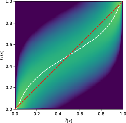
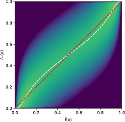
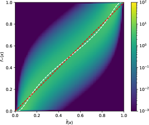
Figure 6: Plots of the density of $(\hat{f}_{{\rm erm}}(\bm{x}),f_{\star}(\bm{x}))$ (Left), after Temperature scaling (Middle) and expectation consistency (Right), for the sampling ratio $\nicefrac{{n}}{{d}}=20$ and regularization $\lambda=10^{-4}$. Dashed white lines represent the accuracy as a function of the confidence, the red line is the diagonal. The difference between red and white lines corresponds to the calibration. ECE of $\hat{f}_{{\rm erm}}$ is, from left to right: 2.1 %, 1.2 %, 1.0 %. We have $T_{TS}=1.24,T_{EC}=1.35$.

As discussed above, different recent works [Sur and Candès, 2019, Bai et al., 2021, Clarté et al., 2022b] have derived exact asymptotic formulas for these statistics in different levels of generality for logistic regression. In particular, the following theorem from Clarté et al. [2022b], which considers a general misspecified model will be used for the analysis:

Theorem 1 (Thm. 3.2 from Clarté et al. [2022b]).

Consider the logit classifier (8) trained by minimizing the empirical risk (9) on a data set $(\bm{x}_{i},y_{i})_{i\in[n]}$ independently sampled from model (5). Then, in the high-dimensional limit when $n,d\to\infty$ at fixed $\alpha=\nicefrac{{n}}{{d}}$:

$$(\nicefrac{{1}}{{d}}\bm{w}_{\star}^{\top}\hat{\bm{w}}_{{\rm erm}},\nicefrac{{1}}{{d}}||\hat{\bm{w}}_{{\rm erm}}||^{2}_{2})\xrightarrow[d\to\infty]{}(m,q)$$ (11)

where $(m,q)\in\mathbb{R}_{+}^{2}$ are explicitly given by the solution of a set of low-dimensional self-consistent equations depending only on $(\alpha,\lambda,\sigma,\sigma_{*})$, and which for the sake of space are discussed in Appendix B.

Leveraging on Thm. 1, we can derive an asymptotic characterization for the asymptotic limit of the uncertainty metrics defined in (2).

Proposition 1.

Under the same assumptions of Theorem 1, the asymptotic limit of the uncertainty metrics defined in (2) is given by:

$$\begin{cases}\Delta_{\ell}(m,q)&=\ell-\mathcal{Z}_{\star}(1,\nicefrac{{m}}{{q}}\sigma^{-1}(\ell),1-\nicefrac{{m^{2}}}{{q}})\\ {\rm ECE}(m,q)&=\int_{0}^{\infty}{\rm d}z|\Delta_{\sigma(z)}(m,q)|\mathcal{N}(z|0,q)\\ \end{cases}$$

where $(m,q)\in\mathbb{R}^{2}_{+}$ are the asymptotic limits of the correlation functions in (11) and

$$\mathcal{Z}_{\star}(y,\omega,V)=\mathbb{E}_{\xi\sim\mathcal{N}(\omega,V)}\left[\sigma_{\star}\left(\nicefrac{{y\xi}}{{T_{\star}}}\right)\right]$$ (12)

The proof of this result is given in Appendix B. Proposition 1 provides us with all we need to fully characterize the calibration properties of TS and EC in our setting. In the next paragraphs, we discuss its implications.

In practice, the $\ell_{2}$ regularization parameter $\lambda$ in the empirical risk (9) is optimized by cross-validation. Clarté et al. [2022b, a] has shown that appropriately regularizing the risk not only improves the prediction accuracy but also the calibration and ECE of the logistic classifier. In particular, it was shown that cross-validating on the loss function yields different results from cross-validation on the misclassification error, with a larger difference arising in the case of misspecified models. Curiously, Clarté et al. [2022a] has shown that in this case, good performance and calibration can be achieved by combining a $\ell_{2}$ penalty with TS. In the following, we discuss how this compares with EC. Note that the exact asymptotic characterization from Thm. 1 allows us to bypass cross-validation, allowing us to find the optimal $\lambda$ by directly optimizing the low-dimensional formulas. We thus define $\lambda_{\rm error}$ (respectively $\lambda_{\rm loss}$) as the value of $\lambda$ such that $\bm{w}_{{\rm erm}}$ yields the lowest test misclassification error (respectively test loss).

5.3 EC outperforms TS

In Section 4, we have numerically observed that EC and TS yield almost the same temperature and thus have similar performance in terms of different uncertainty quantification metrics for different architectures trained on real data sets. Figure 5 shows the relative difference $\delta T=\nicefrac{{|T_{TS}-T_{EC}|}}{{T_{TS}}}$ between the two methods for logistic regression on the synthetic data model (5) for the different choice of target activation $\sigma_{\star}\in\{\sigma_{{\rm logit}},\sigma_{{\rm affine}},\sigma_{{\rm constant}}\}$ defined in (10). Contrary to the real data scenario in Section 4, we observe a significant difference between the two methods for $\sigma_{\star}\in\{\sigma_{{\rm affine}},\sigma_{{\rm constant}}\}$. For instance, for the piece-wise constant function $\sigma_{\star}=\sigma_{{\rm constant}}$, $\delta T$ is a non-decreasing function of the sampling ratio $\alpha$, and is around $30\%$ at $\alpha=20$.

Figure 4 shows that expectation consistency yields a lower ECE than Temperature scaling in all the settings considered in Section 5. On one hand, the effect is small in the well-specified case where the target and model likelihoods are the same: the ECE of Temperature scaling is higher by around $0.01\%$. This is quite intuitive from the discussion in Section 5.1, since in this case, we are closer to the Bayesian setting where both methods were shown to coincide. On the other hand, this difference increases in the misspecified setting, suggesting that model misspecification plays an important role in these calibration methods. In particular, note that in all cases considered here, EC has a lower ECE than TS for all three regularizations considered: $\lambda=10^{-4},\lambda_{\rm error},\lambda_{\rm loss}$.

Figure 6 shows the joint probability density function of the variables $(f_{\star}(\bm{x}),\hat{f}_{{\rm erm}}(\bm{x}))\in[0,1]^{2}$. In particular, we show in white-dashed lines the conditional mean $\mathbb{E}\left[f_{*}(\bm{x})|\hat{f}_{{\rm erm}}(\vec{x})\right]$ which corresponds to the accuracy-confidence chart in Figure 2. As in the real data case, we observe that the ERM estimator is consistently overconfident, i.e $\forall\ell\geqslant\nicefrac{{1}}{{2}},\Delta_{\ell}\geqslant 0$. Moreover, we see that after TS and EC, the conditional mean gets closer to the diagonal (red curve), implying that the model is more calibrated. The phenomenology of the simple data model seems to correspond to what we observe with real data and suggests that expectation consistency is a better approach to calibration.

Interpretation of the results —

Temperature scaling corresponds to rescaling the outputs of the network by minimizing the validation loss. In the literature, the cross-entropy loss is one of the most widespread choices, both for training and for measuring uncertainty scores (with the softmax). From a Bayesian perspective, minimizing the cross-entropy loss corresponds to maximizing the likelihood under the assumption that the has been generated from a softmax (a.k.a. multinomial logit) model. Hence, the underlying assumption behind temperature scaling is that the labels are generated using a softmax likelihood. Therefore, we expect it to perform better when this assumption is met. Indeed, our experiments in Section 5 confirm this intuition. In the case where the ground truth model is indeed given by a logit, TS performs well and is close to EC. However, in the misspecified case, where this assumption does not hold, TS performs worse than EC.

6 Conclusion and future work

In this work, we introduced Expectation Consistency, a new post-training calibration method for neural networks. We have shown that EC is close to temperature scaling across different image classification tasks, giving almost the same expected calibration error and Brier score, while having comparable computational cost. Additionally, we provided an analysis of the asymptotic properties of both methods in a synthetic setting where data is generated by a ground truth model, showing that while EC and TS yield the same performance for well-specified methods, EC provides a better and more principled calibration method under model misspecification.

Our experiments on simple data models showed that when there is a discrepancy between our linear model and the true data model, EC performs better than TS. However, our experiments on real data show a very similar performance across different architectures, data models and overall model accuracy. In future work we aim to understand better why both methods are so similar in practical scenarios.

7 Acknowledgements

We acknowledge funding from the ERC under the European Union’s Horizon 2020 Research and Innovation Program Grant Agreement 714608-SMiLe, the Swiss National Science Foundation grant SNFS OperaGOST, $200021\_200390$ and the Choose France - CNRS AI Rising Talents program. This research was supported by the NCCR MARVEL, a National Centre of Competence in Research, funded by the Swiss National Science Foundation (grant number 205602).

Appendix A Details on training procedure

SVHN

For the SVHN dataset Netzer et al. [2011], the Resnet20 model of depth 20 and containing 0.27M parameters was trained for $50$ epochs, using SGD with a learning rate $\eta=0.1$, weight decay $1e-4$ and momentum $0.9$. $90\%$ of data points were used for training and the rest was used for validation.

CIFAR10

ResNet models (of depth 20, 56 with Resnet56 having 0.85M parameters) were trained for $50$ epochs, using SGD with a learning rate $\eta=0.1$, weight decay $1e-4$ and momentum $0.9$. The DenseNet 121 (containing 7.9 parameters) was trained with the same parameters as the ResNets, except for the learning rate $\eta=0.01$. As in He et al. [2016], images in the training set were randomly cropped and flipped horizontally.

CIFAR100

On CIFAR100, we used pre-trained models from the Github repository https://github.com/chenyaofo/pytorch-cifar-models. These models were trained on the entirety of the training set, so the test set containing $10000$ images was split in half into a validation and test set, containing $5000$ images each.

A.1 Additional plots

In Figure 7, we plot the reliability diagram of Resnet20 and Resnet56 on SVHN and CIFAR10 respectively. We observe that the uncalibrated models are overconfident (as the confidence is higher than the corresponding accuracy), and both TS and EC mitigate this overconfidence.

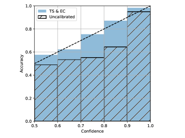
Figure 7: Reliability diagram of Resnet20 on the SVHN dataset (Left) and Resnet56 on the CIFAR10 dataset (Right). Before calibration, both methods are overconfident. TS and EC improve calibration and mitigate overconfidence.

Appendix B State evolution equation

In this section, we focus on the data model introduced in Section 5. Recall that we consider a dataset of $n$ samples $\mathcal{D}=(x^{\mu},y^{\mu})_{\mu=1}^{n}$ generated by

$$\vec{x}\sim\mathcal{N}(\vec{0},\mathcal{I}_{d}/d),\vec{w}_{*}\sim\mathcal{N}(\vec{0},\mathcal{I}_{d}),\mathbb{P}(y=1|\bm{w}_{*}^{\top}\vec{x})=\sigma_{\star}(\bm{w}_{*}^{\top}\vec{x})$$ (13)

and we fit the following logistic regression model, with $\sigma$ the sigmoid function:

$$\hat{f}_{{\rm erm}}(\vec{x})=\sigma(\bm{w}_{{\rm erm}}^{\top}\vec{x})$$ (14)

by minimizing the following empirical risk

$$\mathcal{R}(\vec{w},\mathcal{D},\lambda)=\sum_{\mu=1}^{n}\log\sigma(y^{\mu}\vec{w}^{\top}\vec{x})+\nicefrac{{\lambda}}{{2}}\|\vec{w}\|^{2}$$ (15)

we thus have $\bm{w}_{{\rm erm}}=\arg\min_{\vec{w}}\mathcal{R}(\vec{w},\mathcal{D},\lambda)$. For a new sample $\vec{x}$, we are interested in the joint distribution of $f_{*}(\vec{x})$ and $\hat{f}_{{\rm erm}}(\vec{x})$. As these two functions only depend on the scalar products $\bm{w}_{*}^{\top}\vec{x}$, $\bm{w}_{{\rm erm}}^{\top}\vec{x}$ it suffices to compute the joint distribution of these scalar products. By the Gaussianity of $\vec{x}$, we just need to compute the overlaps $m=\bm{w}_{*}^{\top}\bm{w}_{{\rm erm}}$ and $q=\|\bm{w}_{{\rm erm}}\|^{2}$. In the high-dimensional limit where $n,d\to\infty$ but where we keep the sampling ratio constant $\nicefrac{{n}}{{d}}=\alpha$, it is possible to compute the value of $m$ and $q$. The idea is to introduce the distribution

$$\mu_{\beta,\mathcal{D},\lambda}(\vec{w})=\frac{1}{\mathcal{Z}_{\beta}}\exp\left(-\beta\mathcal{R}(\vec{w},\mathcal{D},\lambda)\right)$$ (16)

where $\mathcal{Z}_{\beta}$ is a normalization constant. In the limit $\beta\to\infty$, $\mu_{\beta,\mathcal{D},\lambda}$ converges to a Dirac distribution peaked at $\bm{w}_{{\rm erm}}=\arg\min\mathcal{R}(\vec{w},\mathcal{D},\lambda)$. To compute $m,q$, one needs to compute the expression of $\log\mathcal{Z}_{\beta}$ and its limit when $\beta\to\infty$. In the high-dimensional regime where both the dimension and number of samples diverge with a fixed ratio, this can be done using the replica method from statistical physics Zdeborová and Krzakala [2016]. As these computations are not the focus of the present paper, we refer to Loureiro et al. [2021], Clarté et al. [2022b] for the detailed computations. In the end, if we define

$$\mathcal{Z_{*}}(y,\omega,v_{*}) =\int{\rm d}z\sigma_{*}(y\times z)\mathcal{N}(z|\omega,v_{*})$$ (17)

$$f(y,\omega,v) =\arg\min_{z}\left[\frac{(z-\omega)^{2}}{2v}-\log\sigma(z)\right]$$ (18)

then $m,q$ are the solution of the following self-consistent equations:

$$\begin{cases}m&=\frac{\hat{m}}{\lambda+\hat{v}}\\ q&=\frac{\hat{q}+\hat{m}^{2}}{(\lambda+\hat{v})^{2}}\\ v&=\frac{1}{\lambda+\hat{v}}\end{cases},\quad\begin{cases}\hat{m}&=\alpha\mathbb{E}_{\xi\sim\mathcal{N}(0,q)}\left[\int{\rm d}y\partial_{\omega}\mathcal{Z}_{*}(y,\nicefrac{{m}}{{q}}\xi,v_{*})f(y,\xi,v)\right]\\ \hat{q}&=\alpha\mathbb{E}_{\xi\sim\mathcal{N}(0,q)}\left[\int{\rm d}y\mathcal{Z}_{*}(y,\nicefrac{{m}}{{q}}\xi,v_{*})f^{2}(y,\xi,v)\right]\\ \hat{v}&=-\alpha\mathbb{E}_{\xi\sim\mathcal{N}(0,q)}\left[\int{\rm d}y\mathcal{Z}_{*}(y,\nicefrac{{m}}{{q}}\xi,v_{*})\partial_{\omega}f(y,\xi,v)\right]\end{cases}$$ (19)

with $v_{*}=\rho-\nicefrac{{m^{2}}}{{q}}$.

Calibration in the high-dimensional regime

Once we obtained the overlaps $m,q$, we can derive the expression the calibration $\Delta_{\ell}$:

$$\Delta_{\ell} =\mathbb{E}\left[f_{*}(\bm{x})|\hat{f}_{{\rm erm}}(\bm{x})\right]=\mathbb{P}\left[y=1|\hat{f}_{{\rm erm}}(\bm{x})\right]=\int{\rm d}z\sigma_{\star}(z)\mathcal{N}(z|\frac{m}{q}\hat{f}_{{\rm erm}}^{-1}(\bm{x}),\rho-\nicefrac{{m^{2}}}{{q}})$$ (20)

The second line comes from the fact that the scalar product $\bm{w}_{*}^{\top}\vec{x}$ conditioned on $\bm{w}_{{\rm erm}}^{\top}\vec{x}=\sigma^{-1}(\ell)$ follows a Gaussian distribution with mean $\nicefrac{{m}}{{q}}\xi$ and variance $\rho-\nicefrac{{m^{2}}}{{q}}$. As a consequence, the expression of ECE is

$$ECE =\mathbb{E}_{\vec{x}}\left[|\Delta_{\hat{f}_{{\rm erm}}(\vec{x})}|\right]=\mathbb{E}_{\xi=\bm{w}_{{\rm erm}}^{\top}\vec{x}}\left[|\Delta_{\sigma(\xi)}|\right]=\int{\rm d}\xi|\Delta_{\sigma(\xi)}|\mathcal{N}(\xi|0,q)$$ (21)

Appendix C Experiments on corrupted dataset

We describe below an experiment where EC can significantly improve over TS for real data: we train different architectures on several image classification tasks, as in Figure 1. However, here for the validation and test set some classes are replaced with random labels. For SVHN and CIFAR10, the labels $y=0$ are replaced by random labels. For CIFAR100, the labels $y=0,...,9$ are replaced by random labels. By doing so, around 10% of validation/test data is corrupted, with a noise that depends on the class. Note that the training data is left unchanged: the goal of this experiment is to model a distribution shift between training and test data, similarly as what is done hendrycks_benchmarking_2019.

In the table below, we compare the performance (in ECE and Brier score) of EC and TS with these corrupted datasets. We observe that in this setting, EC outperforms TS by a significant margin on several datasets and architectures.

Dataset	Model	$\mathcal{E}_{g}$	$T_{TS}$	$T_{EC}$	$ECE$	​​​​ $ECE_{TS}$ ​​​​	​​​​$ECE_{EC}$ ​​​​	​​​​ $BS$ ​​​​	​​​​$BS_{TS}$ ​​​​	​​​​$BS_{EC}$ ​​​​
SVHN	Resnet20	12.5 %	2.69	2.23	8.3 %	10.7 %	7.5 %	21.9 %	23.4 %	22.1 %
CIFAR10	Resnet20	20.9 %	2.4	2.0	12.8 %	4.6 %	4.2 %	34.2 %	32.2 %	32.1 %
CIFAR10	Resnet56	21 %	2.58	2.15	13.8 %	5.4 %	4.9 %	35.2 %	32.9 %	32.8 %
CIFAR10	Densenet121	20.4 %	2.76	2.54	15.8 %	3.6 %	5.0 %	35.9 %	31.8 %	31.9 %
CIFAR100	Resnet20	38.1 %	2.04	1.70	16.5 %	9.6 %	5.9 %	57.0 %	54.9 %	53.9 %
CIFAR100	Resnet56	34.8 %	2.27	2.10	21.7 %	7.6 %	7.3 %	56.0 %	50.6 %	50.4 %
CIFAR100	VGG19	35.5 %	2.6	2.1	28.34 %	5.2	5.1 %	61.8 %	50.1 %	50.1 %
CIFAR100	RepVGG-A2	30.5 %	1.44	1.40	13.7 %	11.6 %	11.7 %	47.2 %	47.1 %	47.0 %

Table 1: Comparison of expected calibration error (ECE) and Brier score (BS) of temperature scaling (TS) and expectation consistency (EC) when part of the validation and test data has been corrupted

References

- Abdar et al. [2021] Moloud Abdar, Farhad Pourpanah, Sadiq Hussain, Dana Rezazadegan, Li Liu, Mohammad Ghavamzadeh, Paul Fieguth, Xiaochun Cao, Abbas Khosravi, U. Rajendra Acharya, Vladimir Makarenkov, and Saeid Nahavandi. A review of uncertainty quantification in deep learning: Techniques, applications and challenges. Information Fusion, 76:243–297, 2021.
- Bai et al. [2021] Yu Bai, Song Mei, Huan Wang, and Caiming Xiong. Don’t just blame over-parametrization for over-confidence: Theoretical analysis of calibration in binary classification. In Marina Meila and Tong Zhang, editors, Proceedings of the 38th International Conference on Machine Learning, volume 139 of Proceedings of Machine Learning Research, pages 566–576. PMLR, 18–24 Jul 2021.
- Clarté et al. [2022a] Lucas Clarté, Bruno Loureiro, Florent Krzakala, and Lenka Zdeborová. A study of uncertainty quantification in overparametrized high-dimensional models, 2022a.
- Clarté et al. [2022b] Lucas Clarté, Bruno Loureiro, Florent Krzakala, and Lenka Zdeborová. Theoretical characterization of uncertainty in high-dimensional linear classification, 2022b.
- Decelle et al. [2011] Aurelien Decelle, Florent Krzakala, Cristopher Moore, and Lenka Zdeborová. Asymptotic analysis of the stochastic block model for modular networks and its algorithmic applications. Physical Review E, 84(6):066106, 2011.
- Dempster et al. [1977] Arthur P Dempster, Nan M Laird, and Donald B Rubin. Maximum likelihood from incomplete data via the em algorithm. Journal of the royal statistical society: series B (methodological), 39(1):1–22, 1977.
- Ding et al. [2021] Xiaohan Ding, Xiangyu Zhang, Ningning Ma, Jungong Han, Guiguang Ding, and Jian Sun. Repvgg: Making vgg-style convnets great again. In Proceedings of the IEEE/CVF conference on computer vision and pattern recognition, pages 13733–13742, 2021.
- Frenkel and Goldberger [2021] Lior Frenkel and Jacob Goldberger. Network calibration by class-based temperature scaling. In 2021 29th European Signal Processing Conference (EUSIPCO), pages 1486–1490, 2021.
- Gal and Ghahramani [2016] Yarin Gal and Zoubin Ghahramani. Dropout as a bayesian approximation: Representing model uncertainty in deep learning. In Proceedings of the 33rd International Conference on International Conference on Machine Learning - Volume 48, 2016.
- Gawlikowski et al. [2021] Jakob Gawlikowski, Cedrique Rovile Njieutcheu Tassi, Mohsin Ali, Jongseok Lee, Matthias Humt, Jianxiang Feng, Anna Kruspe, Rudolph Triebel, Peter Jung, Ribana Roscher, Muhammad Shahzad, Wen Yang, Richard Bamler, and Xiao Xiang Zhu. A survey of uncertainty in deep neural networks, 2021.
- Graves [2011] Alex Graves. Practical variational inference for neural networks. In J. Shawe-Taylor, R. Zemel, P. Bartlett, F. Pereira, and K.Q. Weinberger, editors, Advances in Neural Information Processing Systems, volume 24. Curran Associates, Inc., 2011.
- Guo et al. [2017] Chuan Guo, Geoff Pleiss, Yu Sun, and Kilian Q. Weinberger. On calibration of modern neural networks. In Doina Precup and Yee Whye Teh, editors, Proceedings of the 34th International Conference on Machine Learning, volume 70 of Proceedings of Machine Learning Research, pages 1321–1330. PMLR, 06–11 Aug 2017.
- Gupta et al. [2020] Chirag Gupta, Aleksandr Podkopaev, and Aaditya Ramdas. Distribution-free binary classification: Prediction sets, confidence intervals and calibration. In Proceedings of the 34th International Conference on Neural Information Processing Systems, NIPS’20, Red Hook, NY, USA, 2020. Curran Associates Inc.
- He et al. [2016] K. He, X. Zhang, S. Ren, and J. Sun. Deep residual learning for image recognition. In 2016 IEEE Conference on Computer Vision and Pattern Recognition (CVPR), pages 770–778, Los Alamitos, CA, USA, jun 2016. IEEE Computer Society.
- Huang et al. [2017] G. Huang, Z. Liu, L. Van Der Maaten, and K. Q. Weinberger. Densely connected convolutional networks. In 2017 IEEE Conference on Computer Vision and Pattern Recognition (CVPR), pages 2261–2269, Los Alamitos, CA, USA, jul 2017. IEEE Computer Society.
- Iba [1999] Yukito Iba. The nishimori line and bayesian statistics. Journal of Physics A: Mathematical and General, 32(21):3875, 1999.
- Kristiadi et al. [2020] Agustinus Kristiadi, Matthias Hein, and Philipp Hennig. Being bayesian, even just a bit, fixes overconfidence in ReLU networks. In Hal Daumé III and Aarti Singh, editors, Proceedings of the 37th International Conference on Machine Learning, volume 119 of Proceedings of Machine Learning Research, pages 5436–5446. PMLR, 13–18 Jul 2020.
- Krizhevsky [2009] Alex Krizhevsky. Learning multiple layers of features from tiny images. In Technical report, University of Toronto, 2009.
- Krzakala et al. [2012] Florent Krzakala, Marc Mézard, Francois Sausset, Yifan Sun, and Lenka Zdeborová. Probabilistic reconstruction in compressed sensing: algorithms, phase diagrams, and threshold achieving matrices. Journal of Statistical Mechanics: Theory and Experiment, 2012(08):P08009, 2012.
- Kull et al. [2019] Meelis Kull, Miquel Perello-Nieto, Markus Kängsepp, Telmo Silva Filho, Hao Song, and Peter Flach. Beyond temperature scaling: Obtaining well-calibrated multiclass probabilities with dirichlet calibration. In Proceedings of the 33rd International Conference on Neural Information Processing Systems, Red Hook, NY, USA, 2019. Curran Associates Inc.
- Lakshminarayanan et al. [2017a] Balaji Lakshminarayanan, Alexander Pritzel, and Charles Blundell. Simple and scalable predictive uncertainty estimation using deep ensembles. In Proceedings of the 31st International Conference on Neural Information Processing Systems, NIPS’17, page 6405–6416, Red Hook, NY, USA, 2017a. Curran Associates Inc.
- Lakshminarayanan et al. [2017b] Balaji Lakshminarayanan, Alexander Pritzel, and Charles Blundell. Simple and scalable predictive uncertainty estimation using deep ensembles. In I. Guyon, U. Von Luxburg, S. Bengio, H. Wallach, R. Fergus, S. Vishwanathan, and R. Garnett, editors, Advances in Neural Information Processing Systems, volume 30. Curran Associates, Inc., 2017b.
- Loureiro et al. [2021] Bruno Loureiro, Cedric Gerbelot, Hugo Cui, Sebastian Goldt, Florent Krzakala, Marc Mezard, and Lenka Zdeborová. Learning curves of generic features maps for realistic datasets with a teacher-student model. In M. Ranzato, A. Beygelzimer, Y. Dauphin, P.S. Liang, and J. Wortman Vaughan, editors, Advances in Neural Information Processing Systems, volume 34, pages 18137–18151. Curran Associates, Inc., 2021.
- Maddox et al. [2019] Wesley J. Maddox, T. Garipov, Pavel Izmailov, Dmitry P. Vetrov, and Andrew Gordon Wilson. A simple baseline for bayesian uncertainty in deep learning. In NeurIPS, 2019.
- Mattei [2019] Pierre-Alexandre Mattei. A parsimonious tour of bayesian model uncertainty, 2019.
- Méasson et al. [2009] Cyril Méasson, Andrea Montanari, Thomas J Richardson, and Rüdiger Urbanke. The generalized area theorem and some of its consequences. IEEE Transactions on Information Theory, 55(11):4793–4821, 2009.
- Minderer et al. [2021] Matthias Minderer, Josip Djolonga, Rob Romijnders, Frances Hubis, Xiaohua Zhai, Neil Houlsby, Dustin Tran, and Mario Lucic. Revisiting the Calibration of Modern Neural Networks. In M. Ranzato, A. Beygelzimer, Y. Dauphin, P. S. Liang, and J. Wortman Vaughan, editors, Advances in Neural Information Processing Systems, volume 34, pages 15682–15694. Curran Associates, Inc., 2021.
- Netzer et al. [2011] Yuval Netzer, Tao Wang, Adam Coates, Alessandro Bissacco, Bo Wu, and Andrew Y. Ng. Reading digits in natural images with unsupervised feature learning. In NIPS Workshop on Deep Learning and Unsupervised Feature Learning 2011, 2011.
- Papadopoulos et al. [2002] Harris Papadopoulos, Kostas Proedrou, Volodya Vovk, and Alex Gammerman. Inductive confidence machines for regression. In Machine Learning: ECML 2002: 13th European Conference on Machine Learning Helsinki, Finland, August 19–23, 2002 Proceedings 13, pages 345–356. Springer, 2002.
- Platt [2000] John Platt. Probabilistic outputs for support vector machines and comparisons to regularized likelihood methods. Adv. Large Margin Classif., 10, 06 2000.
- Simonyan and Zisserman [2014] Karen Simonyan and Andrew Zisserman. Very deep convolutional networks for large-scale image recognition. CoRR, abs/1409.1556, 2014.
- Sur and Candès [2019] Pragya Sur and Emmanuel J. Candès. A modern maximum-likelihood theory for high-dimensional logistic regression. Proceedings of the National Academy of Sciences, 116(29):14516–14525, 2019.
- Wang et al. [2021] Deng-Bao Wang, Lei Feng, and Min-Ling Zhang. Rethinking calibration of deep neural networks: Do not be afraid of overconfidence. In Neural Information Processing Systems, 2021.
- Zadrozny and Elkan [2001] Bianca Zadrozny and Charles Elkan. Obtaining calibrated probability estimates from decision trees and naive bayesian classifiers. ICML, 1, 05 2001.
- Zdeborová and Krzakala [2016] Lenka Zdeborová and Florent Krzakala. Statistical physics of inference: Thresholds and algorithms. Advances in Physics, 65(5):453–552, 2016.