Discretization of non-uniform rational B-spline (NURBS) models for meshless isogeometric analysis

Abstract

We present an algorithm for fast generation of quasi-uniform and variable density spatial nodes on domains whose boundaries are represented as computer-aided design (CAD) models, more specifically non-uniform rational B-splines (NURBS). This new algorithm enables the solution of partial differential equations (PDEs) within the volumes enclosed by these CAD models using (collocation-based) meshless numerical discretizations. Our hierarchical algorithm first generates quasi-uniform node sets directly on the NURBS surfaces representing the domain boundary, then uses the NURBS representation in conjunction with the surface nodes to generate nodes within the volume enclosed by the NURBS surface. We provide evidence for the quality of these node sets by analyzing them in terms of local regularity and separation distances. Finally, we demonstrate that these node sets are well-suited (both in terms of accuracy and numerical stability) for meshless radial basis function generated finite differences (RBF-FD) discretizations of the Poisson, Navier-Cauchy, and heat equations. Our algorithm constitutes an important first in bridging the field of node generation for meshless discretizations with mesh generation for isogeometric analysis.

Key words: meshless, CAD, RBF-FD, advancing front algorithms, NURBS

1 Introduction

The key element of any numerical method for solving partial differential equations (PDE) is discretization of the domain. In traditional numerical methods such as the finite element method (FEM), this discretization is typically performed by partitioning the domain into a mesh, i.e., a finite number of elements that entirely cover it. Despite substantial developments in the field of mesh generation, the process of meshing often remains the most time consuming part of the whole solution procedure while the mesh quality limits the accuracy and stability of the numerical solution [18]. In contrast, meshless methods for PDEs work directly on point clouds; in this context, point clouds typically referred to as “nodes”. In particular, meshless methods based on radial basis function generated finite difference (RBF-FD) formulas allow for high-order accurate numerical solutions of PDEs on complicated time-varying domains [29, 14] and even manifolds [26]. The generation of suitable nodes is an area of ongoing research, with much work in recent years [32, 7, 9, 35, 28]. In this work, we focus primarily on the generation of nodes suitable for RBF-FD discretizations, although our node generation approach is fully independent of the numerical method used.

Node sets may be generated in several different ways. For instance, one could simply generate a mesh using an existing tool and discard the connectivity information [17]. However, such an approach is obviously computationally expensive, not easily generalized to higher dimensions, and in some scenarios even fails to generate node distributions of sufficient quality [28]. Another possible approach is to use randomly-generated nodes [17, 22]; this approach has been used (with some modifications) in areas such as compressive sensing [1] and function approximation in high dimensions [24]. Other approaches include iterative optimization [12, 19, 15], sphere-packing [16], QR factorization [34], and repulsion [9, 35]. It is generally accepted that quasi-uniformly-spaced node sets improve the stability of meshless methods [36]. In this context, methods based on Poisson disk sampling are particularly appealing as they produce quasi-uniformly spaced nodes, scale to arbitrary dimension, are computationally efficient, and can be fully automated [28, 32, 7].

A related consideration is the quality of the domain discretization. In the context of meshes, for instance, it is common to characterize mesh quality using element aspect ratios or determinants of Jacobians [11, 38]. Analogously, the node generation literature commonly characterizes node quality in terms of two measures: the minimal spacing between any pair of nodes (the separation distance), and the maximal empty space without nodes (the fill distance). Once again, in this context, Poisson disk sampling via advancing front methods constitutes the state of the art [32, 7]. More specifically, the DIVG algorithm [32] allows for variable-density Poisson disk sampling on complicated domains in arbitrary dimension, while its generalization (sDIVG) allows for sampling of arbitrary-dimensional parametric surfaces. DIVG has since been parallelized [5], distributed as a standalone node generator [30], and is also an important component of the open-source meshless project Medusa [33].

Despite these rapid advances in node generation for meshless methods (and in meshless methods themselves), the generation of node sets on domains whose boundaries are specified by computer aided design (CAD) models is still in its infancy. Consequently, the application of meshless methods in CAD supplied geometries is rare and limited either to smooth geometries [23] or to the use of surface meshes [6, 10, 13]. In contrast, mesh generation and the use of FEM in CAD geometries is a mature and well-understood field [11, 3]. In our experience, current node generation approaches on CAD geometries violate quasi-uniformity near the boundaries and are insufficiently robust or automated for practical use in engineering applications.
In this work, we extend the sDIVG method to the generation of variable-density node sets on parametric CAD surfaces specified by non-uniform rational B-splines (NURBS). We then utilize the variable-density node sets generated by sDIVG in conjunction with the DIVG method to generate node sets in the volume enclosed by the NURBS surface. Our new framework is automated, computationally efficient, scalable to higher dimensions, and generates node sets that retain quasi-uniformity all the way up to the boundary. This framework also inherits the quality guarantees of DIVG and sDIVG, and is consequently well-suited for stable RBF-FD discretizations of PDEs on complicated domain geometries.
The remainder of the paper is organized as follows. The NURBS-DIVG algorithm is presented in Section 2 along with analysis of specific components of the algorithm. The quality of generated nodes is discussed in Section 3. Its application to the RBF-FD solution of PDEs is shown in Section 4. The paper concludes in Section 5.

2 The NURBS-DIVG Algorithm

CAD surfaces are typically described as a union of multiple, non-overlapping, parametric patches (curves in 2D, surfaces in 3D), positioned so that the transitions between them are either smooth or satisfying geometric conditions. A popular choice for representing each patch is a NURBS [27], which is the focus of our work. Here, we present a NURBS-DIVG algorithm that has three primary components:

1. First, we extend the sDIVG algorithm [7] (Section 2.2) for sampling parametric surfaces to sampling individual NURBS patches and also the union of multiple NURBS patches (Section 2.3.2).

2. Next, we deploy the DIVG algorithm [32, 5] in the interior of the domain using the sDIVG generated samples as seed nodes (Section 2.1).

3. To ensure that DIVG generates the correct node sets in the interior of the domain whose boundary consists of multiple parametric NURBS patches, we augment sDIVG with a supersampling parameter (Section 2.3.3).

In following subsections, we first briefly present the DIVG algorithm. We then describe the sDIVG algorithm, which generalizes DIVG to parametric surfaces, focusing on sampling a single NURBS surface. We then describe how the sDIVG algorithm is generalized to surfaces consisting of multiple NURBS patches, each of which have their own boundary curves. Finally, we describe the inside check utilized by our algorithm needed to generate nodes within the NURBS patches, and the complications therein.

2.1 The DIVG algorithm

We now describe the DIVG algorithm for generating node sets within an arbitrary domain. As mentioned previously, this algorithm forms the foundation of the sDIVG and NURBS-DIVG algorithms.

DIVG is an iterative algorithm that begins with a given set of nodes called “seed nodes”; in our case, these will later be provided by NURBS-DIVG. The seed nodes are placed in an expansion queue. In each iteration $i$ of the DIVG algorithm, a single node $\mathbf{p}_{i}$ is dequeued and “expanded”. Here, “expansion” means that a set $C_{i}$ of $n$ candidates for new nodes is uniformly generated on the sphere centered at the node $\mathbf{p}_{i}$, with some radius $r_{i}$ and a random rotation. Here, $r_{i}$ stands for target nodal spacing and can be thought of as derived from a density function $h$, so that $r_{i}=h(\mathbf{p}_{i})$ [32, 31]. Of course, the set $C_{i}$ may contain candidates that lie outside the domain boundary or are too close to an existing node. Such candidates are rejected. However, the candidates that are not rejected are simply added to the domain and to the expansion queue; this is illustrated in Figure 1. The iteration continues until the queue is empty. A full description of DIVG can be found in [32]. Its parallel variant is described in [5].

2.2 The sDIVG algorithm

The sDIVG algorithm is a generalization of DIVG to parametric surfaces. Unlike DIVG (which fills volumes with node sets), sDIVG instead places nodes on a target parametric surface in such a way that the spacing between nodes on the surface follows a supplied density function. While other algorithms typically achieve this through direct Cartesian sampling and elimination [37, 28], the sDIVG algorithm samples the parametric domain corresponding to the surface with an appropriately-transformed version of the supplied density function. More concretely, given a domain $\Omega\subset\mathbb{R}^{d}$, sDIVG iteratively samples its boundary $\partial\Omega\subset\mathbb{R}^{d}$ by sampling a parametrization $\Lambda$ of its boundary instead. The advantage of this approach over direct Cartesian sampling is obtained from the fact that $\Lambda\subset\mathbb{R}^{d-1}$ (or $\mathbb{S}^{d-1}$) is a lower-dimensional representation of $\partial\Omega$, leading to an increase in efficiency.

We now briefly describe the density function transformation utilized by sDIVG. We first define a function $\mathbf{r}:\Lambda\to\partial\Omega$, i.e., a map from the parametric domain $\Lambda\subset\mathbb{R}^{d-1}$ to the manifold $\partial\Omega\subset\mathbb{R}^{d}$; the Jacobian of this function is denoted by $\nabla\mathbf{r}$. As in the DIVG algorithm, let $h$ denote a desired spacing function. Finally, given a node $\boldsymbol{\lambda}_{i}\in\Lambda$, the set of $n$ DIVG-generated candidates for $\boldsymbol{\lambda}_{i}$ can be written as

$$C_{i}=\{\boldsymbol{\eta}_{i,j}\in\Lambda;\ j=1,\ldots,n\}.$$ (1)

It is important to note that the candidates $\boldsymbol{\eta}_{i,j}$ all lie in the parametric domain. Our goal is to determine how far from $\boldsymbol{\lambda}_{i}$ each candidate must lie. From the definition of $\mathbf{r}$ and $h$, we have

$$\|\mathbf{r}(\boldsymbol{\eta}_{i,j})-\mathbf{r}(\boldsymbol{\lambda}_{i})\|=h(\mathbf{r}(\boldsymbol{\lambda}_{i})),$$ (2)

for all $j=1,\ldots,n$. The candidates $\boldsymbol{\eta}_{i,j}$ can be thought of as lying on some manifold around $\boldsymbol{\lambda}_{i}$. This allows us to rewrite $\boldsymbol{\eta}_{i,j}$ as

$$\boldsymbol{\eta}_{i,j}=\boldsymbol{\lambda}_{i}+\alpha_{i,j}\vec{s}_{i,j},$$ (3)

for some $\alpha_{i,j}>0$ and unit vector $\vec{s}_{i,j}$. Here, $\alpha_{i,j}$ must be determined by some appropriate transformation of $h(\mathbf{r}(\boldsymbol{\lambda}_{i}))$, i.e., parametric distances are obtained by a transformation of the spacing function $h$ specified on $\partial\Omega$. We may now use (3) to Taylor expand $\mathbf{r}(\boldsymbol{\eta}_{i,j})$ as

$$\mathbf{r}(\boldsymbol{\eta}_{i,j})=\mathbf{r}(\boldsymbol{\lambda}_{i}+\alpha_{i,j}\vec{s}_{i,j})\approx\mathbf{r}(\boldsymbol{\lambda}_{i})+\alpha_{i,j}\nabla\mathbf{r}(\boldsymbol{\lambda}_{i})\vec{s}_{i,j}.$$ (4)

We can now use (4) in (2) to obtain the following expression for $h(\mathbf{r}(\boldsymbol{\lambda}_{i}))$ in terms of $\alpha_{i,j}$:

$$h(\mathbf{r}(\boldsymbol{\lambda}_{i}))\approx\|\mathbf{r}(\boldsymbol{\lambda}_{i})+\alpha_{i,j}\nabla\mathbf{r}(\boldsymbol{\lambda}_{i})\vec{s}_{i,j}-\mathbf{r}(\boldsymbol{\lambda}_{i})\|=\alpha_{i,j}\|\nabla\mathbf{r}(\boldsymbol{\lambda}_{i})\vec{s}_{i,j}\|.$$ (5)

This in turn allows us to express $\alpha_{i,j}$ as

$$\alpha_{i,j}=\frac{h(\mathbf{r}(\boldsymbol{\lambda}_{i}))}{\|\nabla\mathbf{r}(\boldsymbol{\lambda}_{i})\vec{s}_{i,j}\|}.$$ (6)

We can now use (6) within (1) to obtain an expression for the candidate set $C_{i}$ purely in terms of the spacing function $h$ and the parametric transformation $\mathbf{r}$. Thus, we have

$$C_{i}=\left\{\boldsymbol{\lambda}_{i}+\frac{h(\mathbf{r}(\boldsymbol{\lambda}_{i}))}{\|\nabla\mathbf{r}(\boldsymbol{\lambda}_{i})\vec{s}_{i,j}\|}\vec{s}_{i,j};\vec{s}_{i,j}\in S_{i}\right\},$$ (7)

where $S_{i}$ is set of $n$ random unit vectors on a unit ball. All other steps are identical to DIVG algorithm, albeit in the parametric domain $\Lambda$. The final set of points on $\partial\Omega$ is then obtained by evaluating the function $\mathbf{r}$ at these parametric samples; a schematic of this is shown in Figure 1 (right). A full description of the sDIVG algorithm can be found in [7].

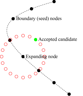
Figure 1: DIVG expansion scheme (left) and sDIVG mapping scheme (right).

2.3 NURBS-DIVG

In principle, sDIVG can be used with any map $\mathbf{r}:\Lambda\to\partial\Omega$. NURBS-DIVG, however, is a specialization of sDIVG to surfaces comprised of NURBS patches (collections of non-overlapping and abutting NURBS). We first describe the use of NURBS for generating the surface representation $\mathbf{r}$, then discuss the generalization to a surface containing multiple patches.

2.3.1 An overview of NURBS surfaces

To define a NURBS representation, it is useful to first define the corresponding B-spline basis in one-dimension. Given a sequence of nondecreasing real numbers $T=\{t_{0},t_{1},\dots,t_{k}\}$ called the knot vector, the degree-$p$ B-spline basis functions $N_{i,p}(u)$ are defined recursively as [27]

$$N_{i,0}(u) =\begin{cases}1;&t_{i}\leq u<t_{i+1}\\ 0;&\text{otherwise}\end{cases}$$ (8)

$$N_{i,p}(u) =\frac{u-t_{i}}{t_{i+p}-t_{i}}N_{i,p-1}(u)+\frac{t_{i+p+1}-u}{t_{i+p+1}-t_{i+1}}N_{i+1,p-1}(u)$$ (9)

We can now use these basis function to define a NURBS curve in $\mathbb{R}^{d}$. Given a knot vector of the form $T=\{\overbrace{a,\dots,a}^{p+1\ \text{times}},t_{p+1},\dots,t_{k-p-1},\overbrace{b,\dots,b}^{p+1\ \text{times}}\}$, $n$ control points $\mathbf{p}_{i}\in\mathbb{R}^{d}$ and $n$ weights $w_{i}\in\mathbb{R}$, the degree-$p$ NURBS curve is defined as [27]

$$\mathbf{s}(u)=\frac{\sum_{i=0}^{n-1}N_{i,p}(u)w_{i}\mathbf{p}_{i}}{\sum_{i=0}^{n-1}N_{i,p}(u)w_{i}},\qquad\text{for}\ a\leq u\leq b.$$ (10)

In practice, it is convenient to evaluate $\mathbf{s}(u)\subset\mathbb{R}^{d}$ as a B-spline curve in $\mathbb{R}^{d+1}$, and then project that curve down to $\mathbb{R}^{d}$. For more details, see [27]. We evaluate the B-spline curve in a numerically stable and efficient fashion using the de Boor algorithm [4], which is itself a generalization of the well-known de Casteljau algorithm for Bezier curves [8]. It is also important to note that derivatives of the NURBS curves with respect to $u$ are needed for computing surface quantities (tangents and normals, for instance, or curvature). Fortunately, it is well-known that these parametric derivatives are also NURBS curves and can therefore also be evaluated using the de Boor algorithm [27]. We adopt this approach in this work.

Finally, the map $\mathbf{r}$ which represents a surface of co-dimension one in $\mathbb{R}^{d}$ can be represented as a NURBS surface; this is merely a tensor-product of two NURBS curves $\mathbf{s}(u)$ and $\mathbf{s}(v)$, where $u$ and $v$ are two independent parameters in $\mathbb{R}^{d-1}$. This allows all NURBS surface operations to be computed via the de Boor algorithm applied to each parametric dimension. The sDIVG algorithm can then be used to sample this surface as desired, which in turn allows for node generation in the interior of the domain via DIVG.

2.3.2 Sampling surfaces consisting of multiple NURBS patches

Practical CAD models typically consist of multiple non-overlapping and abutting NURBS surface patches. A NURBS patch meets another NURBS patch at a NURBS curve (the boundary curves of the respective patches). While degenerate situations can easily arise (such as two NURBS patches intersecting at a single point), we concern ourselves in this work with patches that intersect in NURBS curves. Some examples of node sets generated by NURBS-DIVG on CAD surfaces consisting of multiple NURBS patches are shown in Figure 2.

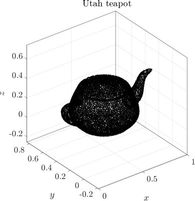
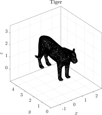
Figure 2: Node sets generated by NURBS-DIVG on a CAD Utah Teapot (left) and a CAD model of tiger (right). The Utah Teapot model is made of 32 patches and has 7031 nodes; the tiger has 124 patches and 4753 boundary nodes.

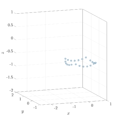
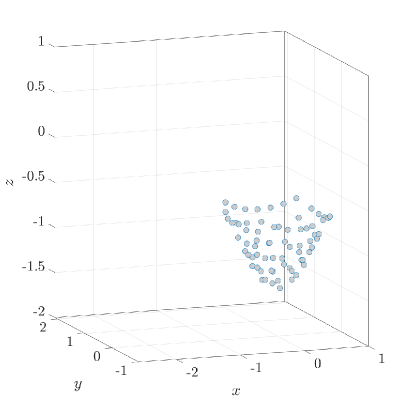
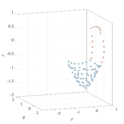
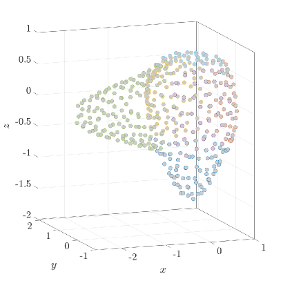
Figure 3: Illustration of positioning nodes on a deformed sphere made of five NURBS patches. In the first step, the boundary of the first patch is filled (first), followed by filling of that patch interior (second). Once the first patch is processed, the boundary of the second patch is discretized (third); this process is repeated until all patches are fully populated with nodes (fourth).

We now describe the next piece of the NURBS-DIVG algorithm: extending sDIVG to discretize a CAD model that consists of several NURBS patches $\partial\Omega_{i}$. We proceed as follows:

1. We use sDIVG to populate patch boundaries $\partial(\partial\Omega_{i})$ with a set of nodes. Recall that these patch boundaries are NURBS curves.

2. We then use these generated nodes as seed nodes within another sDIVG run, this time to fill the NURBS surface patches $\partial\Omega_{i}$ enclosed by those patch boundaries.

To populate patch boundaries, the boundary NURBS representation obtained from any of the intersecting patches can be used. But, to use nodes from patch boundaries as seed nodes in sDIVG for populating surface patches, the corresponding node from the patch’s parametric domain $\Lambda$ is required. While it is possible to determine the map $\Omega\to\Lambda$ through a nonlinear solve, we found it simpler to simply populate the patch boundaries twice, once from each of the NURBS representations obtained from intersecting patches. This produces two sets of seed nodes (one corresponding to each patch), but only the set from one of the representations is used (it does not matter which one, since both node sets are of similar quality). The full process is illustrated in Figure 3.

For a given CAD model consisting of a union of NURBS patches and a desired node spacing $h$, it is possible that the smallest dimension of the patch becomes comparable to (or even smaller) than $h$. We now analyze the behavior of sDIVG in this regime. To do so, we construct simple models comprising of Bezier surfaces (NURBS with constant weights); to emulate the existence of multiple patches, we simply subdivide the Bezier surfaces to obtain patches. In the 3D case, each subdivision is performed in a different direction to ensure patches of similar size. The resulting surface, now a union of non-overlapping and abutting NURBS (Bezier) patches, was then discretized with the NURBS-DIVG algorithm using a uniform spacing of $h=10^{-4}$. We then assessed the quality of the resulting node sets on those patches using the normalized local regularity metric $\overline{d}_{i}^{\prime}$ defined in Section 3. The models and this metric are shown in Figure 4.

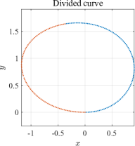
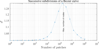
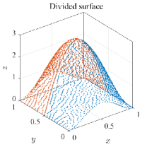
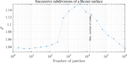
Figure 4: 3D subdivsion analysis

Figure 4 shows that NURBS-DIVG works as expected when $h$ is considerably smaller than the patch size. However, once the patch size becomes comparable to the $h$, the NURBS-DIVG algorithm rejects all nodes except those on the boundaries of the patch, as there is not enough space on the patch itself for additional nodes. In all discussions that follow, we restrict ourselves to the first and most natural regime where $h$ is considerably smaller than the patch size.

2.3.3 NURBS-DIVG in the interior of CAD objects

As our goal is to generate node sets suitable for meshless numerical analysis, it is vital for the NURBS-DIVG algorithm to be able to generate node sets in the interior of volumes whose boundaries are CAD models, in turn defined as a union NURB patches. While it may appear that the original DIVG algorithm is already well-suited to this task, we encountered a problem of nodes “escaping” the domain interior when DIVG was applied naively in the CAD setting. We now explain this problem and the NURBS-DIVG solution more clearly.

To discretize the interior of CAD objects, we must accurately determine whether a particular node lies inside or outside the model. The choice of boundary representation can greatly affect the technique used for such an inside/outside test. For instance, if the domain boundary is modeled as an implicit surface of the form $f({\bf x})=0$, a node ${\bf x}_{k}$ is inside if $f({\bf x}_{k})<0$ (up to some tolerance). However, in the case where the domain boundary is modeled as a parametric surface or a collection of parametric patches (as in this work), the analogous approach would instead solve a nonlinear system of equations to find the parameter values corresponding to ${\bf x}_{k}$ to test if ${\bf x}_{k}$ is inside. A simpler approach used in recent work has been to simply find the closest point from the boundary discretization ${\bf p}$ (with the given spacing $h$) to ${\bf x}_{k}$, and use its unit outward normal to decide if ${\bf x}_{k}$ is inside the domain. More concisely, if ${\bf n}$ is the unit outward normal vector at ${\bf p}$, ${\bf x}_{k}$ is inside the domain $\Omega$ when

$${\bf n}\cdot({\bf x}_{k}-{\bf p})<0.$$ (11)

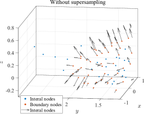
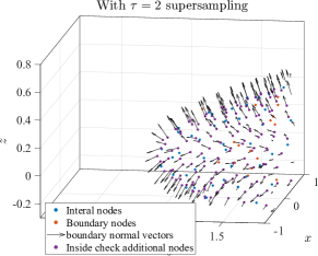
Figure 5: Demonstration of the supersampling approach for the inside/outside test in NURBS-DIVG. The figure on the left shows nodes generated by the naive test used in the DIVG algorithm, with nodes escaping the domain boundary. The figure on the right shows the nodes generated using boundary supersampling in NURBS-DIVG; all non-boundary nodes are enclosed within the volume defined by the boundary.

This is the approach used by the DIVG algorithm (and many others). However, in our experience, this does not work well for complex geometries with sharp edges and concavities. For an illustration, see Figure 5 (left); we see nodes marked as “interior” nodes that are visually outside the convex hull of the boundary nodes.

An investigation revealed that a relatively coarse sampling of a patch near its boundary NURBS curves could result in the closest point ${\bf p}$ and its normal vector $\bf n$ being a bad approximation of the actual closest point and its normal on the domain $\Omega$, thereby resulting in ${\bf x}_{k}$ being erroneously flagged as inside $\Omega$. This problem is especially common on patch boundaries, where normal vectors do not vary smoothly. NURBS-DIVG uses a simple solution: supersampling. More precisely, we use a secondary set of refined boundary nodes only for the inside check with a reduced spacing $\hat{h}$ given by

$$\hat{h}=h/\tau,$$ (12)

where $\tau>1$ is a factor that determines the extent of supersampling. Though this potentially requires $\tau$ to be tuned, this solution worked well in our tests with a minimal additional implementation complexity and computational overhead (see execution profiles for Poisson’s equation in section 4). Figure 5 (right) shows the effect of setting $\tau=2$ in the same domain; nodes no longer “escape” the boundary. While this approach is particularly useful for boundary represented as a collection of NURBS patches, it is likely to be useful in any setting where the boundary has sharp changes in the derivative of the normal vector (or the node spacing $h$). In fact, intuitively, it seems that the greater the derivative (or the smaller the value of $h$), the greater the value of $\tau$ required to prevent nodes escaping.

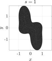
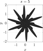
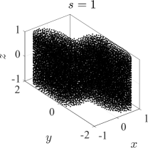
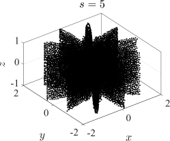
Figure 6: Shapes used to test the supersampling approach in NURBS-DIVG.

To confirm this intuition, we run a simple test both in 2D and 3D. In 2D, we define a parametric curve

$$r(t)=|\cos(st)|^{\sin(2st)},t\in[0,2\pi),$$ (13)

where $s$ is a parameter controlling the complexity of the curve ($s=1$ gives 2 legs, $s=1.5$ gives 3 legs, and so forth). These “legs” create sharp changes in the derivative of the normal (notice $r(t)$ is not smooth in $t$). In 3D, we simply extrude this curve in the $z$ direction to obtain a surface:

$$\mathbf{r}=(r(t)\cos(t),r(t)\sin(t),z),t\in[0,2\pi),z\in[-1,1].$$ (14)

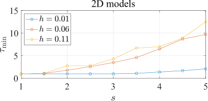
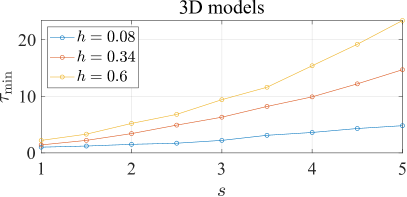
Figure 7: Minimal $\tau$ required to appropriately fill a model.

Both test domains are depicted in Figure 6. We then plot the minimum value of $\tau$ required for a successful inside check as a function of $s$, the parameter that controls the number of legs, and the node spacing $h$. The results are shown in Figure 7. As expected, increasing the number of legs via $s$ necessitates a greater degree of supersampling ($\tau_{min}$ in the plots) in both 2D and 3D. However, if $h$ is sufficiently small to begin with, smaller values of $\tau$ appear to suffice. In the tests presented in later sections, we selected $h$ to be sufficiently small that $\tau=2$ sufficed.

3 Node quality

Although node quality in meshfree context is not as well understood as in mesh based methods, we can analyze local regularity by examining distance distributions to nearest neighbors. For each node $\mathbf{p}_{i}$ with nearest neighbors $\mathbf{p}_{i,j},j=1,\dots c$ we compute

$$\overline{d}_{i}=\frac{1}{c}\sum_{j=1}^{c}||\mathbf{p}_{i}-\mathbf{p}_{i,j}||,$$ (15)

$$d_{i}^{\mathrm{min}}=\min_{j=1,\dots,c}||\mathbf{p}_{i}-\mathbf{p}_{i,j}||,$$ (16)

$$d_{i}^{\mathrm{max}}=\max_{j=1,\dots,c}||\mathbf{p}_{i}-\mathbf{p}_{i,j}||.$$ (17)

and, given a constant $h$, normalize it to $h$.

$$d^{\prime}=d/h.$$ (18)

We used $c=2$ for 2D and $c=3$ for 3D analyses. For the analysis following models are selected

• 2D duck with 8 patches,

• sphere with 6 patches,

• deformed sphere with 6 patches,

all depicted in Figure 8.

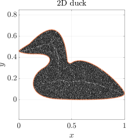
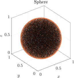
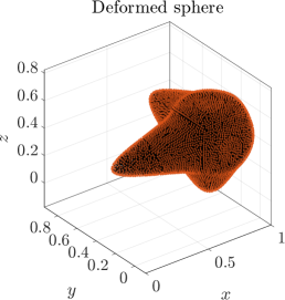
Figure 8: Geometries used in the node quality analysis.

The distance distributions to closest neighbors for boundary nodes are presented in Figure 9 and in Figure 10 distributions for all nodes are shown. The quantitative statistics are presented in Table 1. It can be seen that the nodes are quite uniformly distributed as all distributions are condensed around $1$. In general, the boundary nodes are less uniformly distributed than interior nodes. This is expected, since the Taylor expansion (of the first order) used in sDIVG is an approximation, which means that candidates are not generated exactly at distance $h$ from the node being expanded. This can be improved by using higher order Taylor expansion terms, but in practice, first order expansion is good enough even in complex geometries, where derivatives diverge [7].

Furthermore, in the 2D duck case, the distribution visually seems much better than in the 3D cases. This is a consequence of the candidate generation procedure, which is more optimal when the (parametric) domains are 1D. Another feature characteristic for 1D parametric domains is that outliers with distance to nearest neighbors slightly less than $2h$ are not uncommon. This happens at nodes, where the advancing fronts of the sDIVG algorithm meet and is rarely a problem in practice. Because of that, the standard deviation for duck case shown in Table 1 is of the same order of magnitude as the 3D cases. If 10 most extreme outliers are not taken into account, the standard deviation reduces by an order of magnitude. See [7] for a deeper analysis and possible solutions.

In the 3D cases, the distribution of nodes for the deformed sphere is slightly worse, which can be attributed to a greater complexity of the model. Nevertheless, the quality of generated nodes is of the same order as the nodes generated by pure DIVG [32] and sDIVG [7].

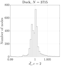
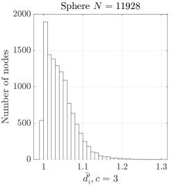
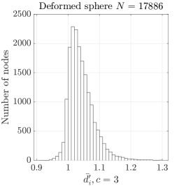
Figure 9: Local regularity distributions for boundary nodes.

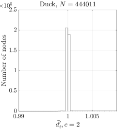
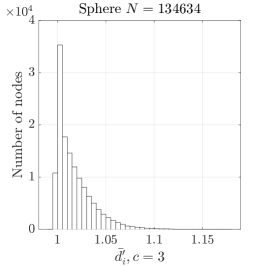
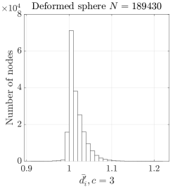
Figure 10: Local regularity distributions for boundary and interior nodes.

Table 1: Statistics.

		$\operatorname{mean}\bar{d}^{\prime}_{i}$	$\operatorname{std}\bar{d}^{\prime}_{i}$	$\operatorname{mean}\left(\left(d_{i}^{\text{max}}\right)^{\prime}-\left(d_{i}^{\text{min}}\right)^{\prime}\right)$
boundary nodes	Duck	$1.0007$	$0.017$	$0.0022$
	Sphere	$1.04$	$0.036$	$0.10$
	Deformed sphere	$1.04$	$0.039$	$0.10$
Boundary and interior nodes	Duck	$1.0032$	$0.013$	$0.0065$
	Sphere	$1.02$	$0.019$	$0.042$
	Deformed sphere	$1.02$	$0.019$	$0.043$

Additionally, there are two quantities often considered as node quality measures, i.e., minimal distance between nodes or separation distance and maximal empty sphere radius within the domain [12, 36]. The separation distance is defined for set of nodes $\Xi=\{x_{1},\dots,x_{N}\}\subset\Omega$ as

$$r_{\mathrm{min},\Xi}=\frac{1}{2}\min_{i\neq j}||\mathbf{x}_{i}-\mathbf{x}_{j}||$$ (19)

and maximal empty sphere radius as

$$r_{\mathrm{max},\Xi}=\sup_{\mathbf{x}\in\Omega}\min_{i}||\mathbf{x}-\mathbf{x}_{i}||.$$ (20)

Quantity $r_{\mathrm{min},\Xi}$ is determined by searching a closest neighbor for all nodes using a spatial search structure, such as a $k$-d tree. A $r_{\mathrm{max},\Xi}$ is estimated numerically by sampling $\Omega$ with higher node density and searching for the closest node among $\Xi$.

Behaviour of normalized maximum empty sphere radius and separation distance for all three cases with respect to target nodal distance $h$ is presented in Figures 11 and 12. In all cases, $r_{\mathrm{max}}$ is relatively stable near an acceptable value of $1$ and $r_{\mathrm{min}}$ approaches the optimal value of $0.5$ with decreasing $h$. This behaviour is consistent with previous results and the analytical bound for $r_{\mathrm{min}}$ [32, 7].

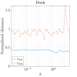
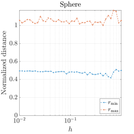
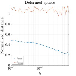
Figure 11: Minimal and maximal spacing on the boundary.

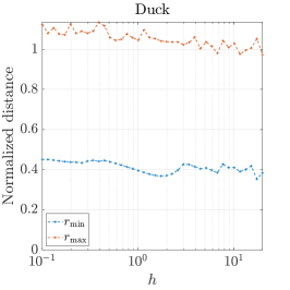
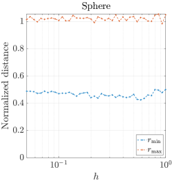
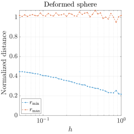
Figure 12: Minimal and maximal spacing on the whole domain.

4 Solving PDEs on CAD geometry

In this section we focus on solving PDEs using the proposed NURBS-DIVG and RBF-FD, a popular variant of strong form local meshless methods. In the first step the CAD provided domain is populated with nodes using NURBS-DIVG that are in the second step used as discretization nodes for a RBF-FD method using polyharmonic basis functions augmented with monomials to approximate considered the PDE [2, 14].

In following numerical experiments we used RBF-FD with augmentation up to order $m\in\{2,4,6\}$ on $n=4\binom{m+2}{2}$ closest nodes in 2D and $n=4\binom{m+3}{3}$ in 3D to obtain the mesh-free approximations of the differential operators involved. The sparse system resulting from discretizing the PDE at hand is solved with BiCGSTAB using an ILUT preconditioner. Note that in all cases we used ghost nodes on boundaries with Neumann or Robin boundary conditions.

4.1 Poisson’s equation

First, we solve a Poisson’s equation

$$\nabla^{2}u=f$$ (21)

with known closed-form solution

$$u_{a}(x,y) =\sin\left(\frac{\pi}{100}x\right)\cos\left(\frac{2\pi}{100}y\right),\quad\text{in 2D},$$ (22)

$$u_{a}(x,y,z) =\sin(\pi x)\cos(2\pi y)\sin(0.5\pi z),\quad\text{in 3D,}$$ (23)

using mixed Neumann-Dirichlet boundary conditions

$$u =u_{a},\quad\text{on }\Gamma_{d},$$ (24)

$$\frac{\partial{u}}{\partial\mathbf{n}} =\frac{\partial{u_{a}}}{\partial\mathbf{n}},\quad\text{on }\Gamma_{n},$$ (25)

where $\Gamma_{d}$ and $\Gamma_{n}$ stand for Dirichlet and Neumann boundaries. In all cases a domain is divided into two halves, where we apply a Dirichlet boundary condition to one half and a Neumann boundary condition to another. The numerical solution of the problem is presented in Figure 13.

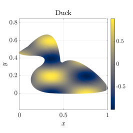
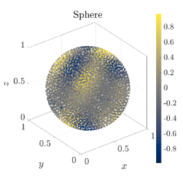
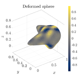
Figure 13: Solution of Poisson’s equation on all three considered geometries.

Once the numerical solution $\hat{u}$ is obtained, we observe the convergence behaviour of the solution through error norms defined as

$$e_{1} =\frac{\|\hat{u}-u_{a}\|_{1}}{\|u_{a}\|_{1}},\quad\|u_{a}\|_{1}=\frac{1}{N}\sum_{i=1}^{N}|u_{a}^{i}|,$$ (26)

$$e_{2} =\frac{\|\hat{u}-u_{a}\|_{2}}{\|u_{a}\|_{2}},\quad\|u_{a}\|_{2}=\sqrt{\frac{1}{N}\sum_{i=1}^{N}|u_{a}^{i}|^{2}},$$ (27)

$$e_{\infty} =\frac{\|\hat{u}-u_{a}\|_{\infty}}{\|u_{a}\|_{\infty}},\quad\|u_{a}\|_{\infty}=\max_{i=1,\ldots,N}|u_{a}^{i}|.$$ (28)

In Figure 14 we can see that for all three geometries the solution converges with the expected order of accuracy according to the order of augmenting monomials.

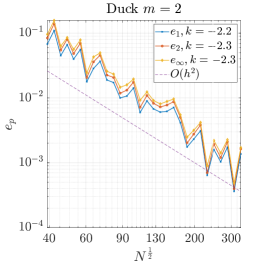
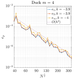
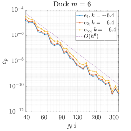
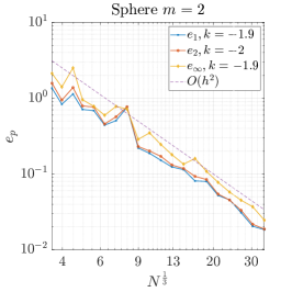
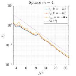
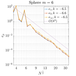
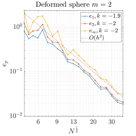
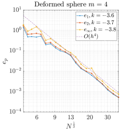
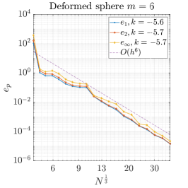
Figure 14: Poisson’s equation solution error with respect to the number of nodes.

Next, we assess the execution time of solving Poisson’s equation with second order monomial augmentation. In Figure 15 the execution times for all three geometries are broken down to core modules of the solution procedure. We separately measure execution time for generation of nodes in interior of the domain (DIVG including inside check with supersampling) and on the surface of the domain (sDIVG on multiple NURBS patches). We measure generation of stencils and computing stencil weights together as a RBF-FD part of the solution procedure. Separately we also measure sparse matrix assembly (which is negligible [5]) and its solution that with increasing number of nodes ultimately dominates the execution time [5]. In 2D duck case the computational times of solving the system and filling the interior of the domain are of the same order as the number of nodes is still relatively small. However, in both 3D cases we can clearly see that solving system scales super-linearly and soon dominates the overall computational cost. The RBF-FD part as expected scales almost linearly (neglecting the $\mathcal{O}(N\log{N})$ resulting from $k$-d tree in stencil selection).

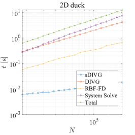
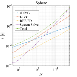
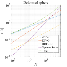
Figure 15: Execution times broken down to separate solution procedure modules.

4.2 Linear elasticity - Navier Cauchy equation

In previous section we established confidence in the presented solution procedure by obtaining expected convergence rates in solving Poisson’s equation on three different geometries in 2D and 3D. In this section we apply NURBS-DIVG to a more realistic case from linear elasticity, governed by the Navier - Cauchy equation

$$\frac{E}{2\left(\nu+1\right)}\left(\nabla^{2}\mathbf{u}+\frac{1}{1-2\nu}\nabla\left({\nabla\cdot\mathbf{u}}\right)\right)=0$$ (29)

where $\mathbf{u}$ stands for the displacement vector, and Young’s modulus $E=$72.1\text{\cdot}{10}^{9}\text{\,}\mathrm{Pa}$$ and Poisson’s ratio $\nu=0.33$ define material properties. The displacement and the stress tensor ($\sigma$) are related via Hooke’s law

$$\sigma=\frac{E}{\nu+1}\left(\frac{1}{1-2\nu}\mathrm{tr}(\varepsilon)I+\varepsilon\right),\quad\varepsilon=\frac{\nabla\bf{u}+(\nabla\mathbf{u})^{\mathsf{T}}}{2},$$ (30)

with $\varepsilon$ and $I$ standing for strain and identity tensors. We observe a 3D gear object that is subjected to an external torque resulting in the tangential traction $t_{0}=$1\text{\cdot}{10}^{3}\text{\,}\mathrm{Pa}$$ on axis, while the gear teeth are blocked, i.e. displacement $\mathbf{u}=$0\text{\,}\mathrm{m}$$. Top and bottom surfaces are free, i.e. traction free boundary conditions apply

$$\bf{u} =$0\text{\,}\mathrm{m}$,\quad\text{on }\Gamma_{\text{teeth}},$$ (31)

$$\sigma\cdot\mathbf{n} =$0\text{\,}\mathrm{Pa}$,\quad\text{on }\Gamma_{\text{free}},$$ (32)

$$\sigma\cdot\mathbf{t} =t_{0}\mathbf{t},\quad\text{on }\Gamma_{\text{axis}}.$$ (33)

The case is schematically presented in Figure 16 together with von Mises stress scatter plot. The stress is highest near the axis, where the force is applied, and gradually fades towards blocked gear teeth. Displacement and von Mises stress are further demonstrated in Figure 17 at $z=$0\text{\,}\mathrm{m}$$ cross section, where we can see how the gear is deformed due to the applied force. Presented results were computed using 41210 scattered nodes generated by NURBS-DIVG.

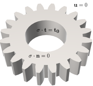
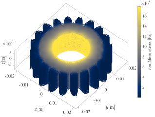
Figure 16: Scheme of the linear elasticity example (left) accompanied with RBF-FD solution in terms of von Misses stress (right).

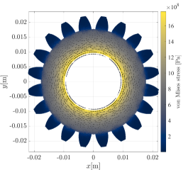
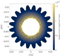
Figure 17: von Mises stress (left) and displacement magnitude (right) at $z=0$ cross section accompanied with quiver plot of displacement field.

4.3 Transient heat transport

Last example is focused on dimensionless transient heat equation

$$\frac{\partial T}{\partial t}=2\nabla^{2}T+q,$$ (34)

where $T$ stands for temperature and q for the heat source. The goal is to solve heat transport within the duck model subjected to the Robin boundary conditions

$$\frac{\partial T}{\partial t}+T=0$$ (35)

and heat source within the domain

$$q=5e^{10||\mathbf{x}-\mathbf{x}_{0}||}$$ (36)

with $\mathbf{x}_{0}=(0,0,0.2)$ and initial temperature set to $0$ throughout the domain. Time marching is performed via implicit stepping using time step $\Delta t=3\cdot 10^{-4}$ and $3000$ iterations to reach the steady state at $t=0.9$

$$T_{2}-\Delta t\nabla^{2}T_{2}=T_{1}+\Delta tq.$$ (37)

Figure 18 shows the temperature scatter plot computed with RBF-FD on 21956 nodes generated with the proposed NURBS-DIVG at two different times (first at the beginning of the simulation and second at the steady state). In Figure 19, the time evolution of the temperature at five control points $P1-5$ is shown. Control point $P1$ is located at the heat source, $P2-4$ at most distant points from the source and $P5$ asymmetric with respect to the y-axis. As one would expect, at the source the temperature rises immediately after the beginning of the simulation and also reaches the highest value, while the rise is a bit delayed and lower at the distant points that are closer to the boundary where the heat exchange with surroundings takes place. Once the heat heat exchange with surrounding matches the heat generation at the source, the system reaches steady-state.

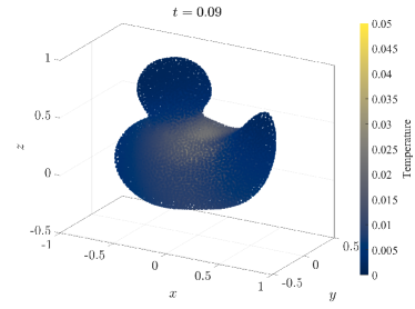
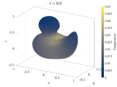
Figure 18: Heat transport within a 3D duck.

Figure 19: Time evolution of temperature at five control points.

5 Conclusions

In this paper, we presented a meshless algorithm, NURBS-DIVG, for generating quasi-uniform nodes on domains whose boundaries are defined by CAD models consisting of multiple NURBS patches. The NURBS-DIVG algorithm is able to deal with complex geometries with sharp edges and concavities, supports refinement, and can be generalized to higher dimensions. We also demonstrated that node layouts generated with NURBS-DIVG are of sufficiently high quality for meshless discretizations, first by directly assessing the quality of these node sets, then by using RBF-FD to solve the Poisson equation with mixed Dirichlet-Neumann boundary conditions on different domains to high-order accuracy. Finally, we demonstrated NURBS-DIVG in conjunction with RBF-FD in tackling two more challenging test cases: first, the stress analysis of a gear subjected to an external force governed by the Navier-Cauchy equation; and second, a time-dependent heat transport problem inside a duck. This work advances the state of the art in fully-autonomous, meshless, isogeometric analysis. All algorithms presented in this work are implemented in C++ and included in our in-house open-source meshfree library Medusa [20, 33], see the Medusa wiki [21] for usage examples. The interface to CAD files was implemented via Open Cascade [25].

References

- [1] B. Adcock, N. Dexter, and Q. Xu, Improved recovery guarantees and sampling strategies for tv minimization in compressive imaging, SIAM Journal on Imaging Sciences, 14 (2021), pp. 1149–1183.
- [2] V. Bayona, N. Flyer, B. Fornberg, and G. A. Barnett, On the role of polynomials in rbf-fd approximations: Ii. numerical solution of elliptic pdes, Journal of Computational Physics, 332 (2017), pp. 257–273.
- [3] J. A. Cottrell, T. J. Hughes, and Y. Bazilevs, Isogeometric analysis: toward integration of CAD and FEA, John Wiley & Sons, 2009.
- [4] C. de Boor, subroutine package for calculating with b-splines., (1971).
- [5] M. Depolli, J. Slak, and G. Kosec, Parallel domain discretization algorithm for rbf-fd and other meshless numerical methods for solving pdes, Computers & Structures, 264 (2022), p. 106773.
- [6] C. Drumm, S. Tiwari, J. Kuhnert, and H.-J. Bart, Finite pointset method for simulation of the liquid–liquid flow field in an extractor, Computers & Chemical Engineering, 32 (2008), pp. 2946–2957.
- [7] U. Duh, G. Kosec, and J. Slak, Fast variable density node generation on parametric surfaces with application to mesh-free methods, SIAM Journal on Scientific Computing, 43 (2021), pp. A980–A1000.
- [8] G. Farin and D. Hansford, The Essentials of CAGD, CRC Press, 2000.
- [9] B. Fornberg and N. Flyer, Fast generation of 2-D node distributions for mesh-free PDE discretizations, Computers & Mathematics with Applications, 69 (2015), p. 531–544.
- [10] S. Gerace, K. Erhart, A. Kassab, and E. Divo, A model-integrated localized collocation meshless method (mims), Computer Assisted Methods in Engineering and Science, 20 (2017), pp. 207–225.
- [11] N. S. Gokhale, Practical finite element analysis, Finite to infinite, 2008.
- [12] D. P. Hardin and E. B. Saff, Discretizing manifolds via minimum energy points, Notices of the AMS, 51 (2004), pp. 1186–1194.
- [13] T. Jacquemin, P. Suchde, and S. P. Bordas, Smart cloud collocation: Geometry-aware adaptivity directly from cad, Computer-Aided Design, (2022), p. 103409.
- [14] M. Jančič, J. Slak, and G. Kosec, Monomial Augmentation Guidelines for RBF-FD from Accuracy Versus Computational Time Perspective, Journal of Scientific Computing, 87 (2021). Publisher: Springer Science and Business Media LLC.
- [15] G. Kosec, A local numerical solution of a fluid-flow problem on an irregular domain, Adv. Eng. Software, 120 (2018), pp. 36–44. Publisher: Elsevier.
- [16] X.-Y. Li, S.-H. Teng, and A. Ungor, Point placement for meshless methods using sphere packing and advancing front methods, in ICCES’00, Los Angeles, CA, Citeseer, 2000.
- [17] G.-R. Liu, Mesh free methods: moving beyond the finite element method, CRC press, 2002.
- [18] G.-R. Liu and Y.-T. Gu, An introduction to meshfree methods and their programming, Springer Science & Business Media, 2005.
- [19] Y. Liu, Y. Nie, W. Zhang, and L. Wang, Node placement method by bubble simulation and its application, Computer Modeling in Engineering and Sciences( CMES), 55 (2010), p. 89.
- [20] Medusa library. http://e6.ijs.si/medusa/, accessed on 15. 12. 2022.
- [21] Medusa wiki. https://e6.ijs.si/medusa/wiki/, accessed on 15. 12. 2022.
- [22] S. Milewski, Higher order schemes introduced to the meshless fdm in elliptic problems, Engineering Analysis with Boundary Elements, 131 (2021), pp. 100–117.
- [23] S. M. Mirfatah, B. Boroomand, and E. Soleimanifar, On the solution of 3d problems in physics: from the geometry definition in cad to the solution by a meshless method, Journal of Computational Physics, 393 (2019), pp. 351–374.
- [24] A. Narayan and D. Xiu, Stochastic collocation methods on unstructured grids in high dimensions via interpolation, SIAM Journal on Scientific Computing, 34 (2012), pp. A1729–A1752.
- [25] Open cascade. http://www.opencascade.com, accessed on 15. 12. 2022.
- [26] A. Petras, L. Ling, and S. J. Ruuth, An rbf-fd closest point method for solving pdes on surfaces, Journal of Computational Physics, 370 (2018), pp. 43–57.
- [27] L. Piegl and W. Tiller, The NURBS book, Springer Science & Business Media, 2012.
- [28] V. Shankar, R. M. Kirby, and A. L. Fogelson, Robust node generation for meshfree discretizations on irregular domains and surfaces, SIAM J. Sci. Comput., 40 (2018), pp. 2584–2608.
- [29] V. Shankar, G. B. Wright, and A. L. Fogelson, An efficient high-order meshless method for advection-diffusion equations on time-varying irregular domains, Journal of Computational Physics, 445 (2021), p. 110633.
- [30] J. Slak and G. Kosec, Standalone implementation of the sequential node placing algorithm. http://e6.ijs.si/medusa/static/PNP.zip.
- [31] , Adaptive radial basis function–generated finite differences method for contact problems, International Journal for Numerical Methods in Engineering, 119 (2019), pp. 661–686. Number: 7 Publisher: Wiley Online Library.
- [32] , On generation of node distributions for meshless PDE discretizations, SIAM Journal on Scientific Computing, 41 (2019), pp. A3202–A3229.
- [33] , Medusa: A c++ library for solving pdes using strong form mesh-free methods, ACM Transactions on Mathematical Software (TOMS), 47 (2021), pp. 1–25.
- [34] P. Suchde, T. Jacquemin, and O. Davydov, Point cloud generation for meshfree methods: An overview, Archives of Computational Methods in Engineering, (2022), pp. 1–27.
- [35] K. van der Sande and B. Fornberg, Fast variable density 3-d node generation, SIAM Journal on Scientific Computing, 43 (2021), pp. A242–A257.
- [36] H. Wendland, Scattered data approximation, no. 17 in Cambridge Monographs on Applied and Computational Mathematics, Cambridge University Press, 2004.
- [37] C. Yuksel, Sample elimination for generating poisson disk sample sets, in Computer Graphics Forum, vol. 34, Wiley Online Library, 2015, pp. 25–32.
- [38] V. Zala, V. Shankar, S. P. Sastry, and R. M. Kirby, Curvilinear mesh adaptation using radial basis function interpolation and smoothing, Journal of Scientific Computing, 77 (2018), pp. 397–418.