Offline Imitation Learning with Suboptimal Demonstrations via
Relaxed Distribution Matching

Abstract

Offline imitation learning (IL) promises the ability to learn performant policies from pre-collected demonstrations without interactions with the environment. However, imitating behaviors fully offline typically requires numerous expert data. To tackle this issue, we study the setting where we have limited expert data and supplementary suboptimal data. In this case, a well-known issue is the distribution shift between the learned policy and the behavior policy that collects the offline data. Prior works mitigate this issue by regularizing the KL divergence between the stationary state-action distributions of the learned policy and the behavior policy. We argue that such constraints based on exact distribution matching can be overly conservative and hamper policy learning, especially when the imperfect offline data is highly suboptimal. To resolve this issue, we present RelaxDICE, which employs an asymmetrically-relaxed $f$-divergence for explicit support regularization. Specifically, instead of driving the learned policy to exactly match the behavior policy, we impose little penalty whenever the density ratio between their stationary state-action distributions is upper bounded by a constant. Note that such formulation leads to a nested min-max optimization problem, which causes instability in practice. RelaxDICE addresses this challenge by supporting a closed-form solution for the inner maximization problem. Extensive empirical study shows that our method significantly outperforms the best prior offline IL method in six standard continuous control environments with over 30% performance gain on average, across 22 settings where the imperfect dataset is highly suboptimal.

Introduction

Imitation learning (IL) (Pomerleau 1988; Ho and Ermon 2016a; Ross, Gordon, and Bagnell 2011) studies the problem of programming agents directly with expert demonstrations. However, successful IL usually demands a large amount of optimal trajectories, and many adversarial IL methods (Ho and Ermon 2016a; Fu, Luo, and Levine 2018; Ke et al. 2020; Kostrikov et al. 2018) require online interactions with the environment to get samples from intermediate policies for policy improvement. Considering these limitations, we focus on the setting of offline imitation learning with supplementary imperfect demonstrations (Kim et al. 2021), which holds the promise of addressing these challenges (i.e. no large collection of expert data and no online interactions with the environment during training). Specifically, we aim to learn a policy using a small amount of expert demonstrations and a large collection of trajectories with unknown level of optimality that are typically cheaper to obtain.

As in prior offline reinforcement learning (RL) and offline policy evaluation works, offline IL (Kim et al. 2021) also has the distribution shift problem (Levine et al. 2020; Kumar et al. 2019; Fujimoto, Meger, and Precup 2018): the agent performs poorly during evaluation because the learned policy deviates from the behavior policy used for collecting the offline data. To mitigate this problem, prior works based on distribution correction estimation (the “DICE” family) (Nachum et al. 2019a, b; Lee et al. 2021; Kim et al. 2021; Kostrikov, Nachum, and Tompson 2020; Zhang et al. 2020; Zhang, Liu, and Whiteson 2020; Yang et al. 2020) collectively use a distribution divergence measure (e.g. $f$-divergence) to regularize the learned policy to be similar to the behavior policy. However, such regularization schemes based on exact distribution matching can be overly conservative. For example, in settings where the offline data is highly suboptimal, such an approach will require careful tuning of the regularization strength (denoted as $\alpha$) in order to find the delicate balance between policy optimization on limited expert data and policy regularization to the behavior policy. Otherwise, the resulting policy will either suffer from large distribution shift because of small $\alpha$ or behave too similarly to the suboptimal behavior policy due to large $\alpha$. We argue that a more appropriate regularization for offline imitation learning with limited expert data and diverse supplementary data is indispensable, which is the goal of this work.

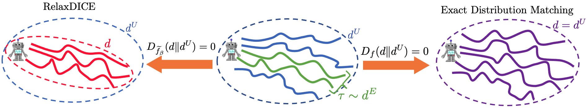
Figure 1: Illustration of regularizations based on relaxed distribution alignment (left) and exact distribution matching (right). The curves represent trajectories sampled from the expert policy (green), the behavior policy that collects the suboptimal data (blue), and the learned policy (red and purple) under different kinds of regularization. Dashed lines represent the support of these distributions.

Towards this end, we draw inspiration from domain adaptation theory (Wu et al. 2019a) and present RelaxDICE, which employs an asymmetrically-relaxed $f$-divergence for explicit support regularization instead of exact distribution matching between the learned policy and the suboptimal behavior policy. On one hand, we still encourage the learned policy to stay within the support of the pre-collected dataset such that policy evaluation/improvement is stable and reliable. On the other hand, we will not drive the learned policy to exactly match the behavior policy since the offline demonstrations have unknown level of optimality (see Figure 1 for illustration). Different from (Wu, Tucker, and Nachum 2019; Levine et al. 2020) which tried to directly regularize the policies and observed little benefits in the context of offline RL, we enforce such a regularization over stationary state-action distributions to effectively reflect the diversity in both states and actions (rather than enforce constraints only on policies/action distributions). However, this leads to a nested min-max optimization problem that causes instability during training. We surprisingly found that our new formulation enjoys a closed-form solution for the inner maximization problem, thus preserving the key advantage of previous state-of-the-art DICE methods (Lee et al. 2021; Kim et al. 2021). Furthermore, the stationary state-action distribution of the suboptimal behavior policy can be potentially modified to be closer to that of the expert policy, by leveraging an approximate density ratio obtained from expert and suboptimal data. Thus we further propose RelaxDICE-DRC, an extension of RelaxDICE by penalizing the relaxed $f$-divergence between the stationary state-action distributions of the learned policy and the density-ratio-corrected behavior policy. This method also enjoys a desirable closed-form solution for the inner maximization and a potential for better policy improvement.

We empirically evaluate our method on a variety of continuous control tasks using environments and datasets from the offline RL benchmark D4RL (Fu et al. 2020). We construct datasets where there are a small amount of expert demonstrations and a large collection of imperfect demonstrations with different levels of optimality following the design choice in (Kim et al. 2021). More importantly, for each environment, we design up to four different settings that are much more challenging than the ones in (Kim et al. 2021), in the sense that the supplementary imperfect data are highly suboptimal. Extensive experimental results show that our method outperforms the most competitive prior offline IL method across all 22 tasks by an average margin over 30%. Furthermore, RelaxDICE is much more performant and robust with respect to hyperparameter changes than prior works (Kim et al. 2021) in our challenging settings, demonstrating the superiority of our relaxed distribution matching scheme for offline imitation learning.

Background

Markov Decision Process.

A Markov decision process (MDP) is defined by ${\mathcal{M}}=\langle{\mathcal{S}},{\mathcal{A}},T,r,p_{0},\gamma\rangle$, where ${\mathcal{S}}$ is a set of states; ${\mathcal{A}}$ is a set of actions; $T:{\mathcal{S}}\times{\mathcal{A}}\to\Delta({\mathcal{S}})$ is the transition distribution and $T(s_{t+1}|s_{t},a_{t})$ specifies the probability of transitioning from state $s_{t}$ to state $s_{t+1}$ by executing action $a_{t}$; $p_{0}\in\Delta({\mathcal{S}})$ is the initial state distribution; $R:{\mathcal{S}}\times{\mathcal{A}}\to{\mathbb{R}}$ is the reward function; and $\gamma\in[0,1]$ is the discount factor. A policy $\pi:{\mathcal{S}}\to\Delta({\mathcal{A}})$ maps from states to distributions over actions, which together with the MDP ${\mathcal{M}}$, induces a stationary state-action distribution $d^{\pi}(s,a)$ (also called occupancy measure):

$$d^{\pi}(s,a)=(1-\gamma)\sum_{t=0}^{\infty}\gamma^{t}\mathrm{Pr}( s_{t}=s,a_{t}=a|s_{0}\sim p_{0},$$

$$a_{t}\sim\pi(\cdot|s_{t}),s_{t+1}\sim T(\cdot|s_{t},a_{t})).$$

Here $1-\gamma$ is a normalization factor such that the occupancy measure is a normalized distribution over ${\mathcal{S}}\times{\mathcal{A}}$. Because of the one-to-one correspondence described in the following theorem, a policy optimization problem can be equivalently formulated as an occupancy measure optimization problem.

Theorem 1 ((Feinberg and Shwartz 2012; Syed, Bowling, and Schapire 2008)).

Suppose $d$ satisfies the following Bellman flow constraints:

$$\sum_{a}d(s,a)=(1-\gamma)p_{0}(s)+\gamma\sum_{s^{\prime},a^{\prime}}T(s|s^{\prime},a^{\prime})d(s^{\prime},a^{\prime}),\forall s.$$

$$\text{and~{}~{}}d(s,a)\geq 0,\forall s,a.$$ (1)

Define $\pi_{d}(a|s)\vcentcolon=\frac{d(s,a)}{\sum_{a^{\prime}}d(s,a^{\prime})}$. Then $d$ is the occupancy measure for $\pi_{d}$. Conversely if $\pi$ is a policy such that $d$ is its occupancy measure, then $\pi=\pi_{d}$ and $d$ satisfies Eq. (1).

The Bellman flow constraints in Eq. (1) essentially characterize all possible occupancy measures consistent with the MDP, such that they can be induced by some policies. Therefore it is necessary to enforce these constraints when we design optimization problems over occupancy measures.

IL with Expert Data.

We can learn performant policies via imitation learning when a set of expert demonstrations ${\mathcal{D}}^{E}$ is provided. The expert dataset ${\mathcal{D}}^{E}=\{(s,a,s^{\prime})\}$ is generated according to $(s,a)\sim d^{E},~{}s^{\prime}\sim T(\cdot|s,a)$, where $d^{E}$ is the occupancy measure of the expert policy. A classical IL approach is behavior cloning (BC), which optimizes a policy $\pi$ by minimizing the expected KL between $\pi^{E}(\cdot|s)$ and $\pi(\cdot|s)$ for $s\sim d^{E}(s)$ (the state marginal of expert occupancy measure):

$$\operatorname*{arg\,min}_{\pi}~{}\mathbb{E}_{d^{E}(s)}\left[D_{\mathrm{KL}}\left(\pi^{E}(\cdot|s)\|\pi(\cdot|s)\right)\right]= -\mathbb{E}_{d^{E}(s,a)}[\log\pi(a|s)].$$

Alternatively, IL can be formulated as minimizing the $f$-divergence between occupancy measures: $\min_{d}D_{f}(d\|d^{E})$ (Ho and Ermon 2016b; Kostrikov, Nachum, and Tompson 2020; Ke et al. 2020; Ghasemipour, Zemel, and Gu 2020). However, since estimating and minimizing $f$-divergence requires the unknown density ratio $d/d^{E}$, which can be obtained only through variational estimation using samples from $d^{E}$ and $d$ (all intermediate policies), these IL methods are not offline and have to use adversarial training.

Offline IL with Expert and Non-Expert Data.

The standard IL setting above typically requires a large amount of optimal demonstrations from experts, and sometimes require online interactions with the MDP. To address these limitations, researchers proposed to study offline IL with limited expert data and supplementary imperfect data (Kim et al. 2021), a meaningful yet challenging setting where no interaction with the environment is allowed, and we only have a small amount of expert demonstrations ${\mathcal{D}}^{E}$ and an additional collection of suboptimal demonstrations ${\mathcal{D}}^{U}$ with unknown level of optimality. The pre-collected dataset ${\mathcal{D}}^{U}=\{(s,a,s^{\prime})\}$ is generated according to $(s,a)\sim d^{U},~{}s^{\prime}\sim T(\cdot|s,a)$ with $d^{U}$ being the occupancy measure of some unknown behavior policy. In this setting, the key is to study how to leverage the additional imperfect dataset ${\mathcal{D}}^{U}$ to provide proper regularization to help the policy/occupancy measure optimization on ${\mathcal{D}}^{E}$. Towards this end, DemoDICE (Kim et al. 2021) extends the offline RL method OptiDICE (Lee et al. 2021) and uses $D_{\mathrm{KL}}(d\|d^{U})$ to realize the regularization. Moreover, we note that a key to their success is both OptiDICE and DemoDICE avoid the nested min-max optimization (Nachum et al. 2019b) by supporting a closed-form solution for their inner maximization problem.

Density Ratio Estimation via Classification.

Thanks to the connection between density ratio estimation and classification (Menon and Ong 2016; Yu, Jin, and Ermon 2021), given samples from two distributions $p$ and $q$, we can use any strictly proper scoring rule and a link function $\psi_{\mathrm{dr}}$ to recover the density ratio $p/q$. For example, we can use logistic regression to approximately recover $d^{E}/d^{U}$:

$$c^{*}=\operatorname*{arg\,max}_{c:{\mathcal{S}}\times{\mathcal{A}}\to(0,1)} \mathbb{E}_{d^{E}(s,a)}[\log c(s,a)]+$$

$$\mathbb{E}_{d^{U}(s,a)}[\log(1-c(s,a))]$$ (2)

Since $c^{*}(s,a)=\frac{d^{E}(s,a)}{d^{E}(s,a)+d^{U}(s,a)}$, the optimal density ratio can be recovered as:

$$r^{*}(s,a)=\psi_{\mathrm{dr}}(c^{*}(s,a))=\frac{c^{*}(s,a)}{1-c^{*}(s,a)}=\frac{d^{E}(s,a)}{d^{U}(s,a)}$$ (3)

Offline IL with Suboptimal Demonstrations via RelaxDICE

In this section, we present RelaxDICE, a novel method for offline imitation learning with expert and supplementary non-expert demonstrations. A key question to study in this meaningful yet challenging setting is how to derive offline algorithms with appropriate regularization $\Omega(d,d^{U})$ to effectively leverage the additional imperfect dataset ${\mathcal{D}}^{U}$. Formally, we begin with the following constrained optimization problem over the occupancy measure:

$$\max_{d\geq 0}~{}-D_{\mathrm{KL}}(d\|d^{E})-\alpha\Omega(d,d^{U})$$ (4)

$$\mathrm{s.t.}~{}~{}\sum_{a}d(s,a)=(1-\gamma)p_{0}(s)+$$

$$~{}~{}~{}~{}~{}~{}~{}~{}~{}~{}~{}~{}~{}~{}~{}~{}~{}~{}~{}~{}~{}~{}~{}~{}~{}~{}~{}~{}~{}~{}~{}~{}\gamma\sum_{s^{\prime},a^{\prime}}T(s|s^{\prime},a^{\prime})d(s^{\prime},a^{\prime}),\forall s\in{\mathcal{S}}.$$ (5)

where Eq. (5) is the Bellman flow constraints introduced in Theorem 1 that any valid occupancy measure must satisfy, and $\alpha>0$ is a weight factor balancing between minimizing KL divergence with $d^{E}$ (estimated with the limited expert data) and preventing deviation from $d^{U}$. For example, a popular regularization choice in prior offline IL and offline RL works is the $f$-divergence $D_{f}(d\|d^{E})$, which was originally designed for exact distribution matching between a model distribution and a target distribution (Nowozin, Cseke, and Tomioka 2016). Although this choice can indeed enforce $d$ to be close to $d^{U}$, we think that divergences or distances for exact distribution matching can be overly conservative and may lead to undesired effects when $d^{U}$ is highly suboptimal. In this case, even the true optimal occupancy measure (corresponding to the true optimal policy) will incur a high penalty from $\Omega(d,d^{U})$. Although we can reduce $\alpha$ to mitigate the negative effect, we cannot remove the bias unless $\alpha$ approaches zero, which will then leave us at risk of exploring out-of-support state-actions because of a too small regularization strength. Moreover, prior theoretical work on offline RL (Zhan et al. 2022) also suggests that a smaller $\alpha$ will lead to a worse sample complexity and a higher error floor. Proofs for this section can be found in the appendix.

An Optimistic Fix to the Pessimistic Regularization

To ensure the suboptimal dataset contains useful information about the optimal policy $\pi^{*}$, theoretical studies typically make some assumptions about ${\mathcal{D}}^{U}$. As a motivating example, a minimal assumption adopted in (Zhan et al. 2022) is the following $\pi^{*}$-concentrability (where $d^{*}$ is the occupancy measure of $\pi^{*}$):

Assumption 1.

$d^{U}(s,a)>0$ and there exists a constant $B$ such that $d^{*}(s,a)/d^{U}(s,a)\leq B,\forall s,a.$

Under this assumption, we argue that an ideal regularization $\Omega(d,d^{U})$ would aim to bound the density ratio $d/d^{U}$ by a constant, instead of driving towards $d\equiv d^{U}$. In other words, we still want to regularize $d$ to stay in the support of $d^{U}$ so that policy evaluation/improvement is stable and reliable under a small distribution shift, but different from a divergence like $D_{f}(d\|d^{U})$, we will impose little penalty on $d$ if $d/d^{U}\leq B$, so that we will not enforce $d$ to exactly match $d^{U}$ and the optimal policy can be preserved under the regularization (i.e., $d^{*}\in\operatorname*{arg\,min}_{d}\Omega(d,d^{U})$).

Towards this end, we draw inspiration from domain adaptation theory (Wu et al. 2019a) and propose to use the following relaxed $f$-divergence to realize $\Omega(d,d^{U})$:

Definition 1 (Asymmetrically-relaxed $f$-divergence).

Given a constant $\beta>1$ and a strictly convex and continuous function $f:{\mathbb{R}}_{+}\to{\mathbb{R}}$ satisfying $f(1)=0$, the asymmetrically-relaxed $f$-divergence between two distributions $p$ and $q$ (defined over domain ${\mathcal{X}}$) is defined as:

$$D_{\widetilde{f}_{\beta}}(p\|q)=\int_{\mathcal{X}}q(x)\widetilde{f}_{\beta}\left(\frac{p(x)}{q(x)}\right)\mathrm{d}x,$$ (6)

where $\widetilde{f}_{\beta}$ is a partially linearized function of $f$ defined as:

$$\widetilde{f}_{\beta}(u)=\begin{dcases}f(u)+C_{f,\beta}&\text{if}~{}~{}u\geq\beta\\ f^{\prime}(\beta)u-f^{\prime}(\beta)&\text{if}~{}~{}u<\beta\end{dcases}$$ (7)

where the constant $C_{f,\beta}\vcentcolon=-f(\beta)+f^{\prime}(\beta)(\beta-1)$.

It is worth noting that $\widetilde{f}_{\beta}$ is also continuous, convex (but not strictly convex) and satisfies $\widetilde{f}_{\beta}(1)=0$. More importantly, $D_{\widetilde{f}_{\beta}}(p\|q)=0$ if and only if $p(x)/q(x)\leq\beta,\forall x\in{\mathcal{X}}$ (proof can be found in the appendix). This property is valuable for IL with suboptimal demonstrations:

Proposition 1.

Under Assumption 1, for any strictly convex function $f$, let $\Omega_{1}(d,d^{U})=D_{f}(d\|d^{U})$ and $\Omega_{2}(d,d^{U})=D_{\widetilde{f}_{\beta}}(d\|d^{U})$ with $\beta=B$. When the behavior policy is not optimal ($d^{U}\neq d^{*}$), then $\Omega_{1}$ is biased while $\Omega_{2}$ preserves the optimal policy (i.e. $d^{*}\notin\operatorname*{arg\,min}_{d}\Omega_{1}(d,d^{U})$ and $d^{*}\in\operatorname*{arg\,min}_{d}\Omega_{2}(d,d^{U})$)

Thus we propose to use the relaxed $f$-divergence to realize the regularization. Let $\Omega(d,d^{U})=D_{\widetilde{f}_{\beta}}(d\|d^{U})$ and we aim to solve the constrained optimization problem in Eq. (4)-(5) in an offline fashion. Apply a change of variable $\omega(s,a)=\frac{d(s,a)}{d^{U}(s,a)}$ to the Lagrangian of above constrained optimization, we can get the following optimization problem over $\omega$ and $v$ (with $v(s)$ being the Lagrange multipliers) (derivations can be found in the appendix):

$$\max_{\omega\geq 0}\min_{v}~{}L_{\alpha,\beta}(\omega,v)\vcentcolon=~{}(1-\gamma)\mathbb{E}_{p_{0}(s)}[v(s)]+$$ (8)

$$\mathbb{E}_{d^{U}(s,a)}\left[\omega(s,a)e_{v}(s,a)-\omega(s,a)\log(\omega(s,a))-\alpha\widetilde{f}_{\beta}(\omega(s,a))\right]$$

Here, $e_{v}(s,a)\vcentcolon=\log\frac{d^{E}(s,a)}{d^{U}(s,a)}+\gamma({\mathcal{T}}v)(s,a)-v(s)$, where the density ratio $d^{E}/d^{U}$ can be estimated via Eq. (2)-(3) and $({\mathcal{T}}v)(s,a)\vcentcolon=\sum_{s^{\prime}}T(s^{\prime}|s,a)v(s^{\prime})$. Note that Eq. (8) can be estimated only using offline datasets ${\mathcal{D}}^{E}$ and ${\mathcal{D}}^{U}$ (assuming ${\mathcal{D}}^{U}$ contains a set of initial states sampled from $p_{0}$).

However, the nested min-max optimization in Eq. (8) usually results in unstable training in practice. To avoid this issue, we follow (Lee et al. 2021; Kim et al. 2021) to assume that every state $s\in{\mathcal{S}}$ is reachable for the given MDP ${\mathcal{M}}$ and thus there exists a strictly feasible $\omega$ such that $\omega(s,a)=d(s,a)/d^{U}(s,a)>0,~{}\forall s,a$. Since Eq. (8) is a convex optimization problem with strict feasibility, due to strong duality via Slater’s condition (Boyd and Vandenberghe 2004), we know that:

$$\max_{\omega\geq 0}\min_{v}~{}L_{\alpha,\beta}(\omega,v)=\min_{v}\max_{\omega\geq 0}~{}L_{\alpha,\beta}(\omega,v)$$ (9)

By changing the max-min problem to min-max problem and using a particular convex function to instantiate the relaxed $f$-divergence, we can obtain the following closed-form solution for the inner maximization problem:

Theorem 2.

Let $D_{\widetilde{f}_{\beta}}$ be the relaxed $f$-divergence in Definition 1, with the associated convex function defined as $f(u)=u\log u$. Then the closed-form solution $\omega^{*}_{v}(s,a)=\operatorname*{arg\,max}_{\omega\geq 0}L_{\alpha,\beta}(\omega,v)$ is:

$$\omega^{*}_{v}(s,a)=$$ (10)

$$\begin{dcases}\exp\left(\frac{e_{v}(s,a)}{1+\alpha}-1\right)&\text{if}~{}~{}\mathfrak{A}(s,a)\\ \exp\left(e_{v}(s,a)-1-\alpha(\log\beta+1)\right)&\text{otherwise}\end{dcases}$$

where $\mathfrak{A}(s,a)$ denotes the event: $\frac{e_{v}(s,a)}{\alpha+1}>\log\beta+1$. Define $h(\omega(s,a))\vcentcolon=\omega(s,a)e_{v}(s,a)-\omega(s,a)\log(\omega(s,a))-\alpha\widetilde{f}_{\beta}(\omega(s,a))$ such that $L_{\alpha,\beta}(\omega,v)=\mathbb{E}_{d^{U}(s,a)}[h(\omega(s,a))]+(1-\gamma)\mathbb{E}_{p_{0}(s)}[v(s)]$. Then we have:

$$h(\omega^{*}_{v}(s,a))=$$

$$\begin{dcases}(1+\alpha)\exp\left(\frac{e_{v}(s,a)}{1+\alpha}-1\right)+C_{1}&\text{if}~{}~{}\mathfrak{A}(s,a)\\ \exp\left(e_{v}(s,a)-1-\alpha(\log\beta+1)\right)+C_{2}&\text{otherwise}\end{dcases}$$

where $C_{1}=-\alpha C_{f,\beta}$ and $C_{2}=\alpha(\log\beta+1)$ are constants w.r.t. $\omega$ and $v$.

Based on Theorem 2, RelaxDICE solves $\hat{v}^{*}=\operatorname*{arg\,min}_{v}L_{\alpha,\beta}(v)=L_{\alpha,\beta}(\omega^{*}_{v},v)$, which provides us a tractable way to leverage a less conservative support regularization to effectively learn from potentially highly suboptimal offline data.

RelaxDICE with Density Ratio Correction

As discussed before, given datasets ${\mathcal{D}}^{E}$ and ${\mathcal{D}}^{U}$, we can obtain an approximate density ratio $\hat{r}(s,a)\approx\frac{d^{E}(s,a)}{d^{U}(s,a)}$. Although we should not expect such an approximate density ratio to be accurate given limited samples, it is likely that the density-ratio-corrected occupancy measure $\hat{r}\cdot d^{U}$ is closer to the expert occupancy measure $d^{E}$ than $d^{U}$. Thus another rational choice for realizing the regularization $\Omega(d,d^{U})$ in Eq. (4) is the relaxed $f$-divergence between $d$ and $\hat{r}\cdot d^{U}$. With this goal, we derive an extension of our method, RelaxDICE with Density Ratio Correction (RelaxDICE-DRC).

Let $\Omega(d,d^{U})=D_{\widetilde{f}_{\beta}}(d\|\hat{r}\cdot d^{U})$. Similar to the derivation of RelaxDICE, we apply a change of variable $\omega(s,a)=\frac{d(s,a)}{d^{U}(s,a)}$ to the Lagrangian of the constrained optimization problem in Eq.(4)-(5) and with strong duality, we can obtain the following min-max optimization problem (derivations in the appendix):

$$\min_{v}\max_{\omega\geq 0}~{}L^{\dagger}_{\alpha,\beta}(\omega,v)\vcentcolon=~{}(1-\gamma)\mathbb{E}_{p_{0}(s)}[v(s)]+$$ (11)

$$\mathbb{E}_{d^{U}(s,a)}\left[\omega(s,a)\left(e_{v}(s,a)-\log(\omega(s,a))\right)-\alpha\hat{r}(s,a)\widetilde{f}_{\beta}\left(\frac{\omega(s,a)}{\hat{r}(s,a)}\right)\right]$$

where $v(s)$ is the Lagrange multiplier and $e_{v}(s,a)$ is defined same as before.

Similar to RelaxDICE, we then introduce the following theorem to characterize the closed-form solution of the inner maximization problem in Eq. (11) to avoid nested min-max optimization:

Theorem 3.

Let $D_{\widetilde{f}_{\beta}}$ be the relaxed $f$-divergence in Definition 1, with $f(u)=u\log u$. Then the closed-form solution $\omega^{*}_{v}(s,a)=\operatorname*{arg\,max}_{\omega\geq 0}L^{\dagger}_{\alpha,\beta}(\omega,v)$ is:

$$\omega^{*}_{v}(s,a)=$$ (12)

$$\begin{dcases}\exp\left(\frac{e_{v}(s,a)+\alpha\log\hat{r}(s,a)}{1+\alpha}-1\right)&\text{if}~{}~{}\mathfrak{B}(s,a)\\ \exp\left(e_{v}(s,a)-1-\alpha(\log\beta+1)\right)&\text{otherwise}\end{dcases}$$

where $\mathfrak{B}(s,a)$ denotes the event: $\frac{e_{v}(s,a)-\log\hat{r}(s,a)}{\alpha+1}>\log\beta+1$. Define $h^{\dagger}(\omega(s,a))\vcentcolon=\omega(s,a)e_{v}(s,a)-\omega(s,a)\log(\omega(s,a))-\alpha\hat{r}(s,a)\widetilde{f}_{\beta}\left(\frac{\omega(s,a)}{\hat{r}(s,a)}\right)$ such that $L^{\dagger}_{\alpha,\beta}(\omega,v)=\mathbb{E}_{d^{U}(s,a)}[h^{\dagger}(\omega(s,a))]+(1-\gamma)\mathbb{E}_{p_{0}(s)}[v(s)]$. Then we have:

$$h^{\dagger}(\omega^{*}_{v}(s,a))=$$

$$\begin{dcases}(1+\alpha)\exp\left(\frac{e_{v}(s,a)+\alpha\log\hat{r}(s,a)}{1+\alpha}-1\right)+C_{3}&\text{if}~{}~{}\mathfrak{B}(s,a)\\ \exp\left(e_{v}(s,a)-1-\alpha(\log\beta+1)\right)+C_{4}&\text{otherwise}\end{dcases}$$

where $C_{3}=-\alpha C_{f,\beta}\hat{r}(s,a)$ and $C_{4}=\alpha(\log\beta+1)\hat{r}(s,a)$ are constants w.r.t. $\omega$ and $v$.

Based on Theorem 3, RelaxDICE-DRC solves $\hat{v}^{*}=\operatorname*{arg\,min}_{v}L^{\dagger}_{\alpha,\beta}(v)=L^{\dagger}_{\alpha,\beta}(\omega^{*}_{v},v)$, which has the potential for better policy learning because of a more well-behaved regularization.

Policy Extraction

Given $v^{*}$, the corresponding density ratio $\hat{\omega}^{*}$ can be recovered according to Eq. (10) (for RelaxDICE) and Eq. (12) (for RelaxDICE-DRC) respectively. We can then use the following weighted BC objective (importance sampling or self-normalized importance sampling) for policy extraction:

$$\max_{\pi}~{}\mathbb{E}_{d^{U}(s,a)}[\hat{\omega}^{*}(s,a)\log\pi(a|s)]~{}~{}\text{or}$$ (13)

$$\max_{\pi}~{}\frac{\mathbb{E}_{d^{U}(s,a)}[\hat{\omega}^{*}(s,a)\log\pi(a|s)]}{\mathbb{E}_{d^{U}(s,a)}[\hat{\omega}^{*}(s,a)]}$$

In practice, we use samples from ${\mathcal{D}}^{U}$ to estimate the expectations and we find that the latter one (using the self-normalized weight) tends to perform better, which we employ in our experiments.

Practical Considerations

Since we only have samples $(s,a,s^{\prime})$ from the dataset ${\mathcal{D}}^{U}$, similar to (Kostrikov, Nachum, and Tompson 2020; Lee et al. 2021; Kim et al. 2021), we have to use a single-point estimation $\hat{e}_{v}(s,a,s^{\prime})=\log\frac{d^{E}(s,a)}{d^{U}(s,a)}+\gamma v(s^{\prime})-v(s)$ for $e_{v}(s,a)$. This estimation is generally biased (when the MDP is stochastic) due to the non-linear exponential function outside of $e_{v}$. However, similar to the observation in (Kostrikov, Nachum, and Tompson 2020), we found this simple approach was enough to achieve good empirical performance on the standard benchmark domains we considered, thus we do not further use the Fenchel conjugate to remove the bias (Nachum et al. 2019a).

We use multilayer perceptron (MLP) networks to parametrize the classifier $c_{\theta}$ in Eq. (2), the Lagrange multiplier $v_{\phi}$, and the policy $\pi_{\psi}$ in Eq. (13). Since the objectives $L_{\alpha,\beta}(v)$ and $L^{\dagger}_{\alpha,\beta}(v)$ contain exponential terms, we use gradient penalty (Gulrajani et al. 2017) to enforce Lipschitz constraints on networks $c_{\theta}$ and $v_{\phi}$, which can effectively stabilize the training. The required density ratio $d^{E}/d^{U}$ in $\hat{e}_{v}$ will be estimated via Eq. (3) as $\hat{r}_{\theta}=\frac{c_{\theta}}{1-c_{\theta}}$.

Regarding the hyperparameter $\beta$, in RelaxDICE, since ideally $\beta$ should be around the upper bound of $d^{E}/d^{U}$, we can automatically set it using the approximate density ratio $\hat{r}_{\theta}$ (e.g., by setting $\beta$ to be the running average of the maximum estimated density ratio of each minibatch); while in RelaxDICE-DRC, $\beta$ should characterize the upper bound of the density ratio $d^{E}/(\hat{r}_{\theta}\cdot d^{U})$, which we expect to be small (e.g.$1.5$ or $2$) as $\hat{r}_{\theta}\cdot d^{U}$ is a density-ratio-corrected occupancy measure. In summary, RelaxDICE does not introduce new hyperparameter that requires tuning by automatically setting $\beta$ according to the data, while RelaxDICE-DRC has the potential for better policy learning with the requirement of manually specifying $\beta$. More details of the practical implementations can be found in the appendix.

Related Work

Learning from imperfect demonstrations.

Imitation learning (Pomerleau 1988; Ross, Gordon, and Bagnell 2011; Ho and Ermon 2016a; Spencer et al. 2021) typically requires many optimal demonstrations, which could be expensive and time-consuming to collect. To address this limitation, imitation learning from imperfect demonstrations (Wu et al. 2019b; Brown et al. 2019; Brown, Goo, and Niekum 2020; Brantley, Sun, and Henaff 2019; Tangkaratt et al. 2020; Wang et al. 2018) arises as a promising alternative.

To do so, prior works assume that the imperfect demonstrations consist of a mixture of expert data and suboptimal data and have considered two-step importance weighted IL (Wu et al. 2019b), learning imperfect demonstrations with adversarial training (Wu et al. 2019b; Wang et al. 2021) and training an ensemble of policies with weighted BC objectives (Sasaki and Yamashina 2020). Note that (Wu et al. 2019b) assumes the access to the optimality labels in the imperfect demonstrations whereas (Wang et al. 2021) and (Sasaki and Yamashina 2020) remove this strong assumption, which is followed in our work. Moreover, (Wu et al. 2019b) and (Wang et al. 2021) require online data collection for policy improvement while our work focuses on learning from offline data.

The closest work to our setting is DemoDICE (Kim et al. 2021), which performs offline imitation learning with a KL constraint to regularize the learned policy to stay close to the behavior policy. Such constraint can mitigate the distribution shift issue when learning from offline data (Levine et al. 2020; Kumar et al. 2019; Fujimoto, Meger, and Precup 2018), but could be overly conservative due to the exact distribution matching regularization especially when the imperfect data is highly suboptimal (see Proposition 1). Our method mitigates this issue by instead using a support regularization. Although (Wu, Tucker, and Nachum 2019) discussed a brief empirical exploration that using support regularization over policies offers little benefits, we instead formulate it as a constrained optimization over occupancy measures to take into consideration the diversity in both states and actions and observed clear practical benefits. Moreover, we surprisingly found that the increased complexity in minimax optimization can be resolved by the convenient closed-form solutions of the inner maximization problems.

Offline learning with stationary distribution correction.

Prior works in offline RL / IL have used distribution correction to mitigate distribtuion shift. AlgaeDICE (Nachum et al. 2019b) leverages a dual formulation of $f$-divergence (Nachum et al. 2019a) to regularize the stationary distribution besides the policy improvement objective in offline RL. ValueDICE (Kostrikov, Nachum, and Tompson 2020) uses a similar formulation to AlgaeDICE for off-policy distribution matching with expert demonstrations. However, both ValueDICE and AlgaeDICE need to solve the nested min-max optimization problem, which is usually unstable in practice. OptiDICE (Lee et al. 2021) and DemoDICE (Kim et al. 2021) resolve this issue via deriving a closed-form solution of their inner optimization problem. Our method also enjoys the same desired property while using an asymmetrically-relaxed $f$-divergence (Wu et al. 2019a) as a more appropriate regularization in face of highly suboptimal offline data.

Experiments

In our experiments, we aim to answer the following three questions: (1) how do RelaxDICE and RelaxDICE-DRC compare to prior works on standard continuous-control tasks using limited expert data and suboptimal offline data? (2) can RelaxDICE remain superior performance compared to prior methods as the quality of the suboptimal offline dataset decreases? (3) can RelaxDICE behave more robustly with respect to different hyperparameter choices compared to prior methods?

						BC-DRC		BC
Envs	Tasks	RelaxDICE	RelaxDICE-DRC	DemoDICE	BCND	$\eta=0.0$	$\eta=0.5$	$\eta=0.0$	$\eta=0.5$	$\eta=1.0$
	L1	74.6$\pm$9.1	73.6$\pm$6.3	70.9$\pm$9.0	6.6$\pm$2.9	1.4$\pm$1.1	2.9$\pm$3.9	1.8$\pm$1.2	7.6$\pm$8.0	17.8$\pm$11.7
	L2	64.2$\pm$8.7	70.0$\pm$13.7	54.4$\pm$6.4	4.8$\pm$4.2	2.4$\pm$1.2	4.9 $\pm$ 2.7	2.9$\pm$2.1	1.6$\pm$1.5	17.8$\pm$11.7
hopper	L3	36.2$\pm$5.6	41.5$\pm$4.3	31.4$\pm$9.7	2.3$\pm$2.3	1.8$\pm$0.5	1.5 $\pm$ 0.6	5.0$\pm$3.3	1.4$\pm$0.9	17.8$\pm$11.7
	L4	38.7$\pm$8.2	40.2$\pm$6.9	34.9$\pm$5.6	0.9$\pm$0.3	0.7$\pm$0.2	1.5$\pm$0.7	0.8$\pm$0.4	0.8$\pm$0.3	17.8$\pm$11.7
	L1	59.1$\pm$8.6	66.7$\pm$5.1	58.6$\pm$8.0	2.5$\pm$0.1	2.6 $\pm$0.0	2.6$\pm$0.0	2.6$\pm$0.0	2.6$\pm$0.0	0.9 $\pm$ 1.1
	L2	49.3$\pm$4.7	52.1$\pm$2.0	48.3$\pm$3.9	2.5$\pm$0.1	2.6 $\pm$0.0	2.6$\pm$0.0	2.6$\pm$0.0	2.6$\pm$0.0	0.9 $\pm$ 1.1
halfcheetah	L3	35.0$\pm$6.6	37.9$\pm$4.0	32.9$\pm$2.1	2.5$\pm$0.0	2.6 $\pm$0.0	2.6$\pm$0.0	2.6$\pm$0.0	2.6$\pm$0.0	0.9 $\pm$ 1.1
	L4	13.3$\pm$2.1	16.1$\pm$4.1	10.5$\pm$0.5	2.6$\pm$0.0	2.6 $\pm$0.0	2.6$\pm$0.0	2.6$\pm$0.0	2.6$\pm$0.0	0.9 $\pm$ 1.1
	L1	92.6$\pm$7.6	99.4$\pm$1.9	98.8$\pm$1.6	3.0$\pm$3.9	0.6$\pm$0.6	0.3$\pm$0.2	2.2$\pm$1.1	0.2$\pm$0.0	8.5$\pm$3.6
	L2	69.7$\pm$20.3	57.7$\pm$12.5	42.1$\pm$23.9	0.1$\pm$0.2	0.2$\pm$0.0	0.5$\pm$0.3	0.2$\pm$0.0	0.3$\pm$0.1	8.5$\pm$3.6
walker2d	L3	41.9$\pm$23.1	56.7$\pm$26.2	23.4$\pm$20.6	0.7$\pm$0.6	0.8$\pm$1.1	0.4$\pm$0.2	0.2$\pm$0.0	0.3$\pm$0.1	8.5$\pm$3.6
	L4	26.3$\pm$17.2	49.5$\pm$17.4	39.8$\pm$22.4	0.2$\pm$0.2	0.2$\pm$0.1	0.5$\pm$0.4	0.2$\pm$0.1	0.2$\pm$0.1	8.5$\pm$3.6
	L1	91.9$\pm$3.6	89.0$\pm$5.3	77.9$\pm$8.7	12.2$\pm$2.4	61.7$\pm$4.9	21.3$\pm$1.2	66.2$\pm$11.2	21.3$\pm$1.1	-8.3$\pm$4.3
	L2	75.2$\pm$5.8	82.1$\pm$7.1	70.5$\pm$4.2	15.6$\pm$2.3	50.8$\pm$6.1	20.6$\pm$1.8	54.4$\pm$4.9	19.9$\pm$1.6	-8.3$\pm$4.3
ant	L3	58.7$\pm$7.1	59.6$\pm$9.0	49.9$\pm$2.9	17.0$\pm$0.9	38.1$\pm$5.2	18.8$\pm$4.7	37.6$\pm$3.0	22.6$\pm$0.1	-8.3$\pm$4.3
	L4	43.2$\pm$7.2	41.3$\pm$4.0	-5.3$\pm$41.4	13.6$\pm$1.7	29.0$\pm$3.9	22.4$\pm$0.2	28.0$\pm$3.1	22.3$\pm$0.3	-8.3$\pm$4.3
	L1	24.2$\pm$17.6	27.3$\pm$13.9	4.1$\pm$3.6	0.2$\pm$0.0	0.4$\pm$0.1	0.3$\pm$0.0	0.4$\pm$0.0	0.3$\pm$0.0	4.8$\pm$2.9
hammer	L2	18.3$\pm$12.0	18.4$\pm$13.6	17.3$\pm$8.9	0.2$\pm$0.0	0.3$\pm$0.0	0.5$\pm$0.4	0.3$\pm$0.1	0.3$\pm$0.0	4.8$\pm$2.9
	L3	19.5$\pm$15.5	20.6$\pm$12.8	14.1$\pm$10.2	0.2$\pm$0.0	0.4$\pm$0.0	0.3$\pm$0.0	0.4$\pm$0.0	0.3$\pm$0.0	4.8$\pm$2.9
	L1	48.0$\pm$2.3	50.9$\pm$5.3	40.9$\pm$13.7	-0.1$\pm$0.0	-0.2$\pm$0.0	6.4$\pm$2.0	-0.2$\pm$0.0	7.3$\pm$2.2	0.2$\pm$0.3
relocate	L2	45.1$\pm$5.7	52.4$\pm$7.7	43.0$\pm$8.2	-0.2$\pm$0.0	5.0$\pm$2.4	-0.2$\pm$0.0	-0.2$\pm$0.0	4.5$\pm$2.1	0.2$\pm$0.3
	L3	39.0$\pm$4.5	43.3$\pm$7.8	27.1$\pm$6.9	-0.2$\pm$0.0	-0.2$\pm$0.0	2.9$\pm$1.9	-0.2$\pm$0.0	3.3$\pm$3.0	0.2$\pm$0.3

Table 1: Results for four MuJoCo environments halfcheetah, hopper, walker2d and ant and two Adroit environments hammer and relocate from D4RL (Fu et al. 2020). Numbers are averaged across 5 seeds, $\pm$ the 95%-confidence interval. We bold the top 2 highest performances. Either RelaxDICE or RelaxDICE-DRC achieves the best performance in each of 22 settings and outperforms the strongest baseline DemoDICE by a large margin in L3 and L4 settings where the offline data is highly suboptimal, suggesting the importance of using a relaxed distribution matching regularization.

Environments, Datasets and Task Construction.

In order to answer these questions, we consider offline datasets of four MuJoCo (Todorov, Erez, and Tassa 2012) locomotion environments (hopper, halfcheetah, walker2d and ant) and two Adroit robotic manipulation environments (hammer and relocate) from the standard offline RL benchmark D4RL (Fu et al. 2020). To construct settings where we have varying data quality of the suboptimal offline dataset, for MuJoCo tasks, we use $1$ trajectory from the expert-v2 datasets as ${\mathcal{D}}^{E}$ for each environment and create the suboptimal offline data ${\mathcal{D}}^{U}$ by mixing $N^{E}$ transitions from expert-v2 datasets and $N^{R}$ transitions from random-v2 datasets with $4$ different ratios. We denote these settings as L1 (Level 1), L2 (Level 2), L3 (Level 3) and L4 (Level 4), which correspond to $\frac{N^{E}}{N^{R}}\approx 0.2,0.15,0.1,0.05$ respectively. The higher the level, the more challenging the setting is. Note that all of the four settings are of much more suboptimal data composition compared to the data configuration used for ${\mathcal{D}}^{U}$ adopted in (Kim et al. 2021), where ${\mathcal{D}}^{U}$ in the most imperfect setting can have $\frac{N^{E}}{N^{R}}>10.0$, e.g. on walker2d. The rationale of constructing such challenging datasets is that in practice, it is much cheaper to generate suboptimal and even random data and therefore a successful offline IL method should be equipped with the capacity of tackling these suboptimal offline datasets. In order to excel at L1, L2, L3 and L4, a successful algorithm must effectively leverage ${\mathcal{D}}^{U}$ to provide proper regularization for policy optimization. For Adroit tasks, following similar design choice, we construct three levels of data compositions, i.e. L1, L2 and L3. Please see the appendix for details.

Comparisons.

To answer these questions, we first consider the following prior approaches. We compare RelaxDICE to DemoDICE (Kim et al. 2021), which performs offline imitation learning with supplementary imperfect demonstrations via applying a KL constraint between the occupancy measure of the learned policy and that of the behavior policy. We also consider BCND (Sasaki and Yamashina 2020) as a baseline, which learns an ensemble of policies via a weighted BC objective on noisy demonstrations. Moreover, we compare to BC$(\eta)$ (Kim et al. 2021), where $\eta\in\{0,0.5,1.0\}$ corresponds to a weight factor that balances between minimizing the negative log-likelihood on expert data ${\mathcal{D}}^{E}$ and minimizing the negative log-likelihood on suboptimal offline data ${\mathcal{D}}^{U}$: $\min_{\pi}L_{\text{BC}(\eta)}(\pi)\vcentcolon=-\eta\frac{1}{|{\mathcal{D}}^{E}|}\sum_{(s,a)\in{\mathcal{D}}^{E}}\log\pi(a|s)-(1-\eta)\frac{1}{|{\mathcal{D}}^{U}|}\sum_{(s,a)\in{\mathcal{D}}^{U}}\log\pi(a|s)$.

Finally, we consider the importance-weighted BC$(\eta)$ denoted as BC-DRC$(\eta)$, i.e. BC with density ratio correction, where we train a classifier to approximate the density ratio $d^{E}/d^{U}$ as $\hat{r}$ via Eq. (2)-(3), and perform weighted BC$(\eta)$ using $\hat{r}$ as the importance weights: $\min_{\pi}L_{\text{BC-DRC}(\eta)}(\pi)\vcentcolon=-\eta\frac{1}{|{\mathcal{D}}^{E}|}\sum_{(s,a)\in{\mathcal{D}}^{E}}\log\pi(a|s)-(1-\eta)\frac{1}{|{\mathcal{D}}^{U}|}\sum_{(s,a)\in{\mathcal{D}}^{U}}\hat{r}(s,a)\log\pi(a|s)$.

For all the tasks, we use $\alpha=0.2$ for RelaxDICE and use $\alpha=0.05$ for DemoDICE as suggested in (Kim et al. 2021), which is also verified in our experiments. We pick $\alpha$ and $\beta$ for RelaxDICE-DRC via grid search, which we will discuss in the appendix. For more details of the experiment set-ups, evaluation protocols, hyperparameters and practical implementations, please see the appendix.

Results of Empirical Evaluations

To answer question (1) and (2), we evaluate RelaxDICE, RelaxDICE-DRC and other approaches discussed above on 6 D4RL environments (4 MuJoCo locomotion tasks and 2 Adroit robotic manipulation tasks) with 22 different settings in total. We present the full results in Table 1.

As shown in Table 1, RelaxDICE-DRC achieves the best performance in 18 out of 22 tasks whereas RelaxDICE excels in the remaining 4 settings. It is also worth noting that RelaxDICE outperforms the strongest baseline DemoDICE in 20 out of 22 settings, without requiring tuning two hyperparameters as in RelaxDICE-DRC. Overall, we observe that the best performing method (either RelaxDICE or RelaxDICE-DRC) achieves over 30% performance improvement on average over DemoDICE. Moreover, in settings where the offline data is highly suboptimal, e.g. L3 and L4, both RelaxDICE and RelaxDICE-DRC can significantly outperform DemoDICE except on walker2d-L4 where RelaxDICE is a bit worse than DemoDICE but RelaxDICE-DRC prevails. In particular, on high-dimensional locomotion tasks such as ant and complex manipulation tasks such as hammer, RelaxDICE and RelaxDICE-DRC outperform DemoDICE by a significant margin on hard datasets such as L3 and L4. These suggest that using a less conservative support regularization can be crucial in cases with extremely low-quality offline data, supporting our theoretical analysis.

Sensitivity of Hyperparameters

To answer question (3), we perform an ablation study on the sensitivity of the hyperparameter $\alpha$ in RelaxDICE and DemoDICE (Kim et al. 2021), which controls the strength of the regularization between the learned policy and the behavior policy. We pick two continuous-control tasks halfcheetah and walker2d and evaluate the performance of RelaxDICE and DemoDICE using $\alpha\in\{0.05,0.1,0.2,0.3,0.4,0.5\}$ on all four settings in each of the two tasks. As shown in Figure 2 in the appendix, RelaxDICE is much more robust w.r.t. $\alpha$ compared to DemoDICE in all of the 8 scenarios as RelaxDICE remains roughly a flat line in all eight plots and the performance of DemoDICE drops significantly as $\alpha$ increases. We think the reason is that DemoDICE employs a conservative exact distribution matching constraint and therefore requires different values of $\alpha$ on datasets with different data quality to find the delicate balance between policy optimization based on limited ${\mathcal{D}}^{E}$ and regularization from suboptimal ${\mathcal{D}}^{U}$, e.g. higher $\alpha$ when the data quality is high and lower $\alpha$ when the data is highly suboptimal. In contrast, RelaxDICE imposes a relaxed support regularization, which is less conservative and therefore less sensitive w.r.t. data quality. Since tuning hyperparameters for offline IL / RL in a fully offline manner remains an open problem and often requires expensive online samples (Monier et al. 2020; Kumar et al. 2021; Yu et al. 2021; Kurenkov and Kolesnikov 2021), we believe RelaxDICE’s robustness w.r.t. the hyperparameters should significantly benefit practitioners.

Conclusion and Discussion

We present RelaxDICE, a novel offline imitation learning methods for learning policies from limited expert data and supplementary imperfect data. Different from prior works using regularizations originally designed for exact distribution matching, we employ an asymmetrically relaxed $f$-divergence as a more forgiving regularization that proves effective even for settings where the imperfect data is highly suboptimal. Both RelaxDICE and its extension RelaxDICE-DRC can avoid unstable min-max optimization of the regularized stationary state-action distribution matching problem by supporting a closed-form solution of the inner maximization problem, and show superior performance to strong baselines in our extensive empirical study.

Appendix A Derivation for RelaxDICE

We propose to use the relaxed $f$-divergence to realize the regularization $\Omega(d,d^{U})$ and aim to solve the following constrained optimization problem in an offline fashion:

$$\max_{d\geq 0}~{}-D_{\mathrm{KL}}(d\|d^{E})-\alpha D_{\widetilde{f}_{\beta}}(d\|d^{U})$$ (14)

$$\mathrm{s.t.}~{}~{}\sum_{a}d(s,a)=(1-\gamma)p_{0}(s)+\gamma\sum_{s^{\prime},a^{\prime}}T(s|s^{\prime},a^{\prime})d(s^{\prime},a^{\prime}),\forall s\in{\mathcal{S}}.$$ (15)

For notation simplicity, we define $({\mathcal{B}}d)(s)\vcentcolon=\sum_{a}d(s,a)$, $({\mathcal{T}}d)(s)\vcentcolon=\sum_{s^{\prime},a^{\prime}}T(s|s^{\prime},a^{\prime})d(s^{\prime},a^{\prime})$ and $({\mathcal{T}}v)(s,a)\vcentcolon=\sum_{s^{\prime}}T(s^{\prime}|s,a)v(s^{\prime})$. First, we can obtain the following Lagrangian for above constrained optimization problem (with $v(s)$ being the Lagrange multipliers):

$$\max_{d\geq 0}\min_{v}~{}L_{\alpha,\beta}(d,v)\vcentcolon= -D_{\mathrm{KL}}(d\|d^{E})-\alpha D_{\widetilde{f}_{\beta}}(d\|d^{U})$$

$$+\sum_{s}v(s)((1-\gamma)p_{0}(s)+\gamma({\mathcal{T}}d)(s)-({\mathcal{B}}d)(s))$$ (16)

Plugging in the definitions of KL divergence and relaxed $f$-divergence in Definition 1, $L_{\alpha,\beta}(d,v)$ in Eq. (16) can be written as:

$$L_{\alpha,\beta}(d,v)= ~{}\mathbb{E}_{d(s,a)}\left[\log\frac{d^{E}(s,a)\cdot d^{U}(s,a)}{d^{U}(s,a)\cdot d(s,a)}\right]-\alpha\mathbb{E}_{d^{U}(s,a)}\left[\widetilde{f}_{\beta}\left(\frac{d(s,a)}{d^{U}(s,a)}\right)\right]$$

$$+(1-\gamma)\mathbb{E}_{p_{0}(s)}[v(s)]+\mathbb{E}_{d(s,a)}[\gamma({\mathcal{T}}v)(s,a)-v(s)]$$ (17)

$$= ~{}\mathbb{E}_{d^{U}(s,a)}\left[\frac{d(s,a)}{d^{U}(s,a)}\left(\log\frac{d^{E}(s,a)}{d^{U}(s,a)}+\gamma({\mathcal{T}}v)(s,a)-v(s)-\log\frac{d(s,a)}{d^{U}(s,a)}\right)\right]$$

$$-\alpha\mathbb{E}_{d^{U}(s,a)}\left[\widetilde{f}_{\beta}\left(\frac{d(s,a)}{d^{U}(s,a)}\right)\right]+(1-\gamma)\mathbb{E}_{p_{0}(s)}[v(s)]$$ (18)

where Eq. (17) uses the fact that $\sum_{s}v(s)({\mathcal{T}}d)(s)=\sum_{s,a}d(s,a)({\mathcal{T}}v)(s,a)$, and the density ratio $d^{E}/d^{U}$ can be estimated via Eq. (2)-(3); and Eq. (18) uses importance sampling to change the expectation w.r.t. $d$ to an expectation w.r.t. $d^{U}$ for offline learning.

Define $e_{v}(s,a)\vcentcolon=\log\frac{d^{E}(s,a)}{d^{U}(s,a)}+\gamma({\mathcal{T}}v)(s,a)-v(s)$ and use a change of variable $\omega(s,a)=\frac{d(s,a)}{d^{U}(s,a)}$, we obtain the following optimization problem:

$$\max_{\omega\geq 0}\min_{v}~{}L_{\alpha,\beta}(\omega,v)\vcentcolon=~{} \mathbb{E}_{d^{U}(s,a)}\left[\omega(s,a)e_{v}(s,a)-\omega(s,a)\log(\omega(s,a))-\alpha\widetilde{f}_{\beta}(\omega(s,a))\right]$$

$$+(1-\gamma)\mathbb{E}_{p_{0}(s)}[v(s)]$$ (19)

which can be estimated only using offline datasets ${\mathcal{D}}^{E}$ and ${\mathcal{D}}^{U}$ (assuming ${\mathcal{D}}^{U}$ additionally contains a set of initial states sampled from $p_{0}$).

Remark. We note that DemoDICE (Kim et al. 2021) is a special case of RelaxDICE when $\beta\to 0$, which can be verified according to Definition 1 and Theorem 2 (we will always be in the first condition of the piecewise function as $\log\beta+1\to-\infty$ when $\beta\to 0$).

Appendix B Derivation for RelaxDICE-DRC

As discussed before, another attractive choice for realizing the regularization is the relaxed $f$-divergence between $d$ and the density-ratio-corrected behavior occupancy measure $\hat{r}\cdot d^{U}$.

Let $\Omega(d,d^{U})=D_{\widetilde{f}_{\beta}}(d\|\hat{r}\cdot d^{U})$ and we aim to solve the following constrained optimization problem in an offline fashion:

$$\max_{d\geq 0}~{}-D_{\mathrm{KL}}(d\|d^{E})-\alpha D_{\widetilde{f}_{\beta}}(d\|\hat{r}\cdot d^{U})$$ (20)

$$\mathrm{s.t.}~{}~{}\sum_{a}d(s,a)=(1-\gamma)p_{0}(s)+\gamma\sum_{s^{\prime},a^{\prime}}T(s|s^{\prime},a^{\prime})d(s^{\prime},a^{\prime}),\forall s\in{\mathcal{S}}.$$ (21)

Similar to the derivation of RelaxDICE, we can obtain the following Lagrangian for the constrained optimization problem in Eq.(20)-(21) (with $v(s)$ being the Lagrange multipliers):

$$L^{\dagger}_{\alpha,\beta}(d,v)= ~{}\mathbb{E}_{d^{U}(s,a)}\left[\frac{d(s,a)}{d^{U}(s,a)}\left(e_{v}(s,a)-\log\frac{d(s,a)}{d^{U}(s,a)}\right)\right]$$

$$-\alpha\mathbb{E}_{d^{U}(s,a)}\left[\hat{r}(s,a)\cdot\widetilde{f}_{\beta}\left(\frac{d(s,a)}{\hat{r}(s,a)\cdot d^{U}(s,a)}\right)\right]+(1-\gamma)\mathbb{E}_{p_{0}(s)}[v(s)]$$ (22)

Similarly, we use a change of variable $\omega(s,a)=\frac{d(s,a)}{d^{U}(s,a)}$ and apply strong duality to obtain the following min-max problem over $\omega$:

$$\min_{v}\max_{\omega\geq 0}~{}L^{\dagger}_{\alpha,\beta}(\omega,v)\vcentcolon=~{} \mathbb{E}_{d^{U}(s,a)}\left[\omega(s,a)e_{v}(s,a)-\omega(s,a)\log(\omega(s,a))-\alpha\hat{r}(s,a)\widetilde{f}_{\beta}\left(\frac{\omega(s,a)}{\hat{r}(s,a)}\right)\right]$$

$$+(1-\gamma)\mathbb{E}_{p_{0}(s)}[v(s)]$$ (23)

Appendix C Proofs

Lemma 1.

For distributions $p$ and $q$ defined on domain ${\mathcal{X}}$, if $\frac{p(x)}{q(x)}<\beta,~{}\forall x\in{\mathcal{X}}$, then the relaxed $f$-divergence $D_{\widetilde{f}_{\beta}}(p\|q)=0$.

Proof.

According to Definition 1, if $p/q<\beta$ everywhere, we have:

$$D_{\widetilde{f}_{\beta}}(p,\|q) =\int_{{\mathcal{X}}}q(x)\widetilde{f}_{\beta}\left(\frac{p(x)}{q(x)}\right)\mathrm{d}x$$

$$=\int_{{\mathcal{X}}}q(x)\left(f^{\prime}(\beta)\frac{p(x)}{q(x)}-f^{\prime}(\beta)\right)\mathrm{d}x$$

$$=f^{\prime}(\beta)\int_{{\mathcal{X}}}p(x)\mathrm{d}x-f^{\prime}(\beta)\int_{{\mathcal{X}}}q(x)\mathrm{d}x=0$$

∎

See 2

Proof.

Since $\widetilde{f}_{\beta}$ is a continuous piecewise function, $h(\omega(s,a))$ is also a continuous piecewise function:

$$h(\omega(s,a)) =\begin{dcases}e_{v}(s,a)\omega(s,a)-\omega(s,a)\log(\omega(s,a))-\alpha f(\omega(s,a))-\alpha C_{f,\beta}&\text{if}~{}~{}\omega(s,a)\geq\beta\\ e_{v}(s,a)\omega(s,a)-\omega(s,a)\log(\omega(s,a))-\alpha f^{\prime}(\beta)\omega(s,a)+\alpha f^{\prime}(\beta)&\text{if}~{}~{}\beta\geq\omega(s,a)\geq 0\end{dcases}$$

When $f(u)=u\log u$ and $f^{\prime}(u)=\log u+1$, the gradient of $h(\omega(s,a))$ is given by:

$$h^{\prime}(\omega(s,a)) =\begin{dcases}e_{v}(s,a)-(\alpha+1)(\log(\omega(s,a))+1)&\text{if}~{}~{}\omega(s,a)\geq\beta\\ e_{v}(s,a)-\log(\omega(s,a))-1-\alpha(\log\beta+1)&\text{if}~{}~{}\beta\geq\omega(s,a)\geq 0\end{dcases}$$

Define $\omega^{*}_{\leq\beta}(s,a)$ and $\omega^{*}_{\geq\beta}(s,a)$ as the local maximum for $[0,\beta]$ and $[\beta,+\infty)$ respectively:

$$\omega^{*}_{\leq\beta}(s,a)\vcentcolon=\operatorname*{arg\,max}_{\beta\geq\omega(s,a)\geq 0}h(\omega(s,a))~{}~{}\text{and}~{}~{}\omega^{*}_{\geq\beta}(s,a)\vcentcolon=\operatorname*{arg\,max}_{\omega(s,a)\geq\beta}h(\omega(s,a))$$

and the overall maximum will be either $\omega^{*}_{\leq\beta}(s,a)$ or $\omega^{*}_{\geq\beta}(s,a)$ depending on whose function value is larger (the global maximum must be one of the local maximums).

In the following, we will use the fact that $h^{\prime}$ is strictly decreasing due to the strict concavity of $h$ (an affine function plus a strictly concave function).

(1) When $e_{v}(s,a)>(\alpha+1)(\log\beta+1)$ (or equivalently $h^{\prime}(\beta)>0$):

For $\beta\geq\omega(s,a)\geq 0$, we know that $h^{\prime}(\omega(s,a))\geq h^{\prime}(\beta)=e_{v}(s,a)-(\alpha+1)(\log\beta+1)>0$, so $\omega^{*}_{\leq\beta}(s,a)=\beta$.

For $\omega(s,a)\geq\beta$, since $h^{\prime}$ is strictly decreasing and $h^{\prime}(\beta)>0$, we know that $\omega^{*}_{\geq\beta}(s,a)$ is attained at $h^{\prime}(\omega(s,a))=e_{v}(s,a)-(\alpha+1)(\log(\omega(s,a))+1)=0$. Thus $\omega^{*}_{\geq\beta}(s,a)=\exp\left(\frac{e_{v}(s,a)}{1+\alpha}-1\right)$.

Moreover, because $h^{\prime}(\omega(s,a))>0$ when $\beta\leq\omega(s,a)<\omega^{*}_{\geq\beta}(s,a)$, we know that $h(\omega^{*}_{\leq\beta}(s,a))=h(\beta)<h(\omega^{*}_{\geq\beta}(s,a))$, and the overall maximum is $\omega^{*}(s,a)=\exp\left(\frac{e_{v}(s,a)}{1+\alpha}-1\right)>\beta$.

In this case, the maximum function value of $h$ is:

$$h(\omega^{*}(s,a)) =e_{v}(s,a)\omega^{*}(s,a)-\omega^{*}(s,a)\log(\omega^{*}(s,a))-\alpha f(\omega^{*}(s,a))-\alpha C_{f,\beta}$$

$$=\omega^{*}(s,a)\left(e_{v}(s,a)-(\alpha+1)\log(\omega^{*}(s,a))\right)-\alpha C_{f,\beta}$$

$$=(\alpha+1)\omega^{*}(s,a)-\alpha C_{f,\beta}$$

$$=(\alpha+1)\exp\left(\frac{e_{v}(s,a)}{1+\alpha}-1\right)-\alpha C_{f,\beta}$$

(2) When $e_{v}(s,a)\leq(\alpha+1)(\log\beta+1)$ (or equivalently $h^{\prime}(\beta)\leq 0$) :

Since $\lim_{\omega(s,a)\to 0}h^{\prime}(\omega(s,a))=+\infty$ and $h^{\prime}(\beta)\leq 0$, $\omega^{*}_{\leq\beta}(s,a)$ is attained at $h^{\prime}(\omega(s,a))=e_{v}(s,a)-\log(\omega(s,a))-1-\alpha(\log\beta+1)=0$. Thus $\omega^{*}_{\leq\beta}(s,a)=\exp\left(e_{v}(s,a)-1-\alpha(\log\beta+1)\right)$.

For $\omega(s,a)\geq\beta$, since $h^{\prime}$ is strictly decreasing and $h^{\prime}(\beta)\leq 0$, so $h^{\prime}(\omega(s,a))\leq 0$ and $\omega^{*}_{\geq\beta}(s,a)=\beta$.

Moreover, because $h(\omega^{*}_{\leq\beta}(s,a))\geq h(\beta)=h(\omega^{*}_{\geq\beta}(s,a))$, the overall maximum is $\omega^{*}(s,a)=\exp\left(e_{v}(s,a)-1-\alpha(\log\beta+1)\right)\leq\beta$.

In this case, the maximum function value of $h$ is:

$$h(\omega^{*}(s,a)) =e_{v}(s,a)\omega^{*}(s,a)-\omega^{*}(s,a)\log(\omega^{*}(s,a))-\alpha f^{\prime}(\beta)\omega^{*}(s,a)+\alpha f^{\prime}(\beta)$$

$$=\omega^{*}(s,a)\left(e_{v}(s,a)-\log(\omega^{*}(s,a))-\alpha(\log\beta+1)\right)+\alpha(\log\beta+1)$$

$$=\omega^{*}(s,a)+\alpha(\log\beta+1)$$

$$=\exp\left(e_{v}(s,a)-1-\alpha(\log\beta+1)\right)+\alpha(\log\beta+1)$$

∎

See 3

Proof.

Since $\widetilde{f}_{\beta}$ is a continuous differentiable piecewise function, $h^{\dagger}(\omega(s,a))$ is also a continuous differentiable piecewise function. When $f(u)=u\log u$ and $f^{\prime}(u)=\log u+1$, we have:

$$h^{\dagger}(\omega(s,a)) =\begin{dcases}e_{v}(s,a)\omega(s,a)-\omega(s,a)\log(\omega(s,a))-\alpha\omega(s,a)\log\left(\frac{\omega(s,a)}{\hat{r}(s,a)}\right)-\alpha C_{f,\beta}\hat{r}(s,a)&\text{if}~{}~{}\frac{\omega(s,a)}{\hat{r}(s,a)}\geq\beta\\ e_{v}(s,a)\omega(s,a)-\omega(s,a)\log(\omega(s,a))-\alpha f^{\prime}(\beta)\omega(s,a)+\alpha f^{\prime}(\beta)\hat{r}(s,a)&\text{if}~{}~{}\beta\geq\frac{\omega(s,a)}{\hat{r}(s,a)}\geq 0\end{dcases}$$

The gradient of $h^{\dagger}(\omega(s,a))$ is given by:

$$(h^{\dagger})^{\prime}(\omega(s,a)) =\begin{dcases}e_{v}(s,a)-(\alpha+1)(\log(\omega(s,a))+1)+\alpha\log\hat{r}(s,a)&\text{if}~{}~{}\omega(s,a)\geq\beta\hat{r}(s,a)\\ e_{v}(s,a)-\log(\omega(s,a))-1-\alpha(\log\beta+1)&\text{if}~{}~{}\beta\hat{r}(s,a)\geq\omega(s,a)\geq 0\end{dcases}$$

Define $\omega^{*}_{\leq\beta\hat{r}}(s,a)$ and $\omega^{*}_{\geq\beta\hat{r}}(s,a)$ as the local maximum for $[0,\beta\hat{r}(s,a)]$ and $[\beta\hat{r}(s,a),+\infty)$:

$$\omega^{*}_{\leq\beta\hat{r}}(s,a)\vcentcolon=\operatorname*{arg\,max}_{\beta\hat{r}(s,a)\geq\omega(s,a)\geq 0}h(\omega(s,a))~{}~{}\text{and}~{}~{}\omega^{*}_{\geq\beta\hat{r}}(s,a)\vcentcolon=\operatorname*{arg\,max}_{\omega(s,a)\geq\beta\hat{r}(s,a)}h(\omega(s,a))$$

and the overall maximum will be either $\omega^{*}_{\leq\beta\hat{r}}(s,a)$ or $\omega^{*}_{\geq\beta\hat{r}}(s,a)$ depending on whose function value is larger (the global maximum must be one of the local maximums).

In the following, we will use the fact that $(h^{\dagger})^{\prime}$ is strictly decreasing due to the strict concavity of $h^{\dagger}$ (an affine function plus a strictly concave function).

(1) When $e_{v}(s,a)>(\alpha+1)(\log\beta+1)+\log\hat{r}(s,a)$ (or equivalently $(h^{\dagger})^{\prime}(\beta\hat{r}(s,a))>0$):

For $\beta\hat{r}(s,a)\geq\omega(s,a)\geq 0$, we know that $(h^{\dagger})^{\prime}(\omega(s,a))\geq(h^{\dagger})^{\prime}(\beta\hat{r}(s,a))=e_{v}(s,a)-(\alpha+1)(\log\beta+1)-\log\hat{r}(s,a)>0$, so $\omega^{*}_{\leq\beta\hat{r}}(s,a)=\beta\hat{r}(s,a)$.

For $\omega(s,a)\geq\beta\hat{r}(s,a)$, since $(h^{\dagger})^{\prime}$ is strictly decreasing and $(h^{\dagger})^{\prime}(\beta\hat{r}(s,a))>0$, we know that $\omega^{*}_{\geq\beta\hat{r}}(s,a)$ is attained at $(h^{\dagger})^{\prime}(\omega(s,a))=e_{v}(s,a)-(\alpha+1)(\log(\omega(s,a))+1)+\alpha\log\hat{r}(s,a)=0$. Thus $\omega^{*}_{\geq\beta\hat{r}}(s,a)=\exp\left(\frac{e_{v}(s,a)+\alpha\log\hat{r}(s,a)}{1+\alpha}-1\right)$.

Moreover, because $h(\omega^{*}_{\leq\beta\hat{r}}(s,a))=h(\beta\hat{r}(s,a))<h(\omega^{*}_{\geq\beta\hat{r}}(s,a))$, and the overall maximum is $\omega^{*}(s,a)=\exp\left(\frac{e_{v}(s,a)+\alpha\log\hat{r}(s,a)}{1+\alpha}-1\right)>\beta\hat{r}(s,a)$.

In this case, the maximum function value of $h$ is:

$$h(\omega^{*}(s,a)) =e_{v}(s,a)\omega^{*}(s,a)-\omega^{*}(s,a)\log(\omega^{*}(s,a))-\alpha\omega^{*}(s,a)\log\left(\frac{\omega^{*}(s,a)}{\hat{r}(s,a)}\right)-\alpha C_{f,\beta}\hat{r}(s,a)$$

$$=\omega^{*}(s,a)\left(e_{v}(s,a)-(\alpha+1)\log(\omega^{*}(s,a))+\alpha\log(\hat{r}(s,a))\right)-\alpha C_{f,\beta}\hat{r}(s,a)$$

$$=(\alpha+1)\omega^{*}(s,a)-\alpha C_{f,\beta}\hat{r}(s,a)$$

$$=(\alpha+1)\exp\left(\frac{e_{v}(s,a)+\alpha\log\hat{r}(s,a)}{1+\alpha}-1\right)-\alpha C_{f,\beta}\hat{r}(s,a)$$

(2) When $e_{v}(s,a)\leq(\alpha+1)(\log\beta+1)+\log\hat{r}(s,a)$ (or equivalently $(h^{\dagger})^{\prime}(\beta\hat{r}(s,a))\leq 0$) :

Since $\lim_{\omega(s,a)\to 0}(h^{\dagger})^{\prime}(\omega)=+\infty$ and $(h^{\dagger})^{\prime}(\beta\hat{r}(s,a))\leq 0$, $\omega^{*}_{\leq\beta\hat{r}}(s,a)$ is attained at $(h^{\dagger})^{\prime}(\omega(s,a))=e_{v}(s,a)-\log(\omega(s,a))-1-\alpha(\log\beta+1)=0$. Thus $\omega^{*}_{\leq\beta\hat{r}}(s,a)=\exp\left(e_{v}(s,a)-1-\alpha(\log\beta+1)\right)$.

For $\omega(s,a)\geq\beta\hat{r}(s,a)$, since $(h^{\dagger})^{\prime}$ is strictly decreasing and $(h^{\dagger})^{\prime}(\beta\hat{r}(s,a))\leq 0$, so $(h^{\dagger})^{\prime}(\omega(s,a))\leq 0$ and $\omega^{*}_{\geq\beta\hat{r}}(s,a)=\beta\hat{r}(s,a)$.

Moreover, because $h(\omega^{*}_{\leq\beta\hat{r}}(s,a))\geq h(\beta\hat{r}(s,a))=h(\omega^{*}_{\geq\beta\hat{r}}(s,a))$, the overall maximum is $\omega^{*}(s,a)=\exp\left(e_{v}(s,a)-1-\alpha(\log\beta+1)\right)$.

In this case, the maximum function value of $h$ is:

$$h(\omega^{*}(s,a)) =e_{v}(s,a)\omega^{*}(s,a)-\omega^{*}(s,a)\log(\omega^{*}(s,a))-\alpha f^{\prime}(\beta)\omega^{*}(s,a)+\alpha f^{\prime}(\beta)\hat{r}(s,a)$$

$$=\omega^{*}(s,a)\left(e_{v}(s,a)-\log(\omega^{*}(s,a))-\alpha(\log\beta+1)\right)+\alpha(\log\beta+1)\hat{r}(s,a)$$

$$=\omega^{*}(s,a)+\alpha(\log\beta+1)\hat{r}(s,a)$$

$$=\exp\left(e_{v}(s,a)-1-\alpha(\log\beta+1)\right)+\alpha(\log\beta+1)\hat{r}(s,a)$$

∎

Appendix D Additional Experimental Results and Details

Sensitivity of Hyperparameters for Controlling Regularization Strength

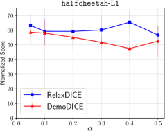
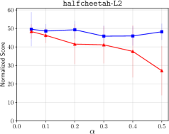
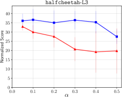
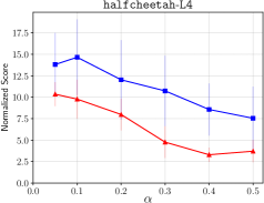
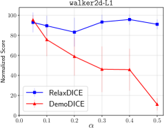
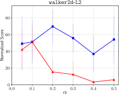
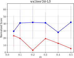
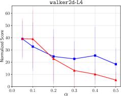
Figure 2: Ablation study on the sensitivity of $\alpha$ for RelaxDICE and DemoDICE (Kim et al. 2021). RelaxDICE is much more robust w.r.t. different values of $\alpha$ compared to DemoDICE across different data compositions.

Task Description

We consider offline datasets of four MuJoCo (Todorov, Erez, and Tassa 2012) locomotion environments (hopper, halfcheetah, walker2d and ant) and two Adroit robotic manipulation environments (hammer and relocate) from the standard offline RL benchmark D4RL (Fu et al. 2020). For each environment, we construct different settings where there is a limited amount of expert demonstrations (denoted as ${\mathcal{D}}^{E}$) and a relatively large collection of suboptimal trajectories (denoted as ${\mathcal{D}}^{U}$) by mixing $N^{E}$ transitions from expert datasets and $N^{R}$ transitions from extremely low-quality datasets. We denote these settings as L1 (Level 1), L2 (Level 2), L3 (Level 3) and L4 (Level 4), where a higher level means a more challenging setting. Note that for Adroit environments, we use three settings L1, L2 and L3 instead of four due to the complexity of the high-dimensional tasks. It’s also worth noting that all the considered tasks here are much more challenging than the settings in (Kim et al. 2021), in the sense that these settings are of much more suboptimal data composition (even tasks L1 have lower $N^{E}/N^{R}$ ratios than the most challenging tasks in (Kim et al. 2021)). We summarize the details of these tasks in Table 2.

		Expert Dataset ${\mathcal{D}}^{E}$	Suboptimal Dataset ${\mathcal{D}}^{U}$
Envs	Tasks	# of transitions from expert-v2	# of transitions from expert-v2	# of transitions from random-v2
	L1	1k	200k	1000k
	L2	1k	150k	1000k
halfcheetah	L3	1k	100k	1000k
	L4	1k	50k	1000k
	L1	1k	14k	22k
	L2	1k	10k	22k
hopper	L3	1k	5k	22k
	L4	1k	2k	22k
	L1	1k	10k	20k
	L2	1k	5k	20k
walker2d	L3	1k	3k	20k
	L4	1k	2k	20k
	L1	1k	30k	180k
	L2	1k	20k	180k
ant	L3	1k	10k	180k
	L4	1k	5k	180k
		Expert Dataset ${\mathcal{D}}^{E}$	Suboptimal Dataset ${\mathcal{D}}^{U}$
Envs	Tasks	# of transitions from expert-v0	# of transitions from expert-v0	# of transitions from cloned-v0
	L1	2k	1000k	1000k
hammer	L2	2k	790k	1000k
	L3	2k	590k	1000k
	L1	10k	1000k	1000k
relocate	L2	10k	790k	1000k
	L3	10k	590k	1000k

Table 2: Dataset statistics for four MuJoCo environments halfcheetah, hopper, walker2d and ant and two Adroit environments hammer and relocate from D4RL (Fu et al. 2020).

Evaluation Protocols

For all the methods except BCND, we run 1M training iterations (gradient steps) and we report the average performance of the last 50k (5%) steps to capture their asymptotic performance at convergence. For BCND, we follow the implementation in Appendix E.1 in (Kim et al. 2021), which has predefined number of iterations according to dataset statistics and we also report the average performance of the last 50k steps for consistent evaluation.

For four MuJoCo locomotion environments halfcheetah, hopper, walker2d and ant, we follow (Kim et al. 2021) to compute the normalized score as:

$$\texttt{normalized\_score}=100\times\frac{\texttt{score}-\texttt{random\_score}}{\texttt{expert\_score}-\texttt{random\_score}}$$

where the expert_score and random_score corresponds to the average return of trajectories in expert-v2 and random-v2 respectively.

For two Adroit environments hammer and relocate, we use the recommended reference score in D4RL to compute the normalized score.

Hyperparameters

Algorithm Hyperparameters

We use $\gamma=0.99$ as the discount factor of the MDP. All methods use a batch size of $256$. The hyperparameters for each of the compared algorithm are summarized below.

• BC: $\eta\in\{0.0,0.5,1.0\}$.

• BC-DRC: $\eta\in\{0.0,0.5\}$.

• BCND: We follow the hyperparameter configurations in Appendix E.1 in (Kim et al. 2021).

• DemoDICE: $\alpha=0.05$ across all tasks, as suggested in (Kim et al. 2021) and verified in our experiments.

• RelaxDICE: $\alpha=0.2$ across all tasks. As shown in Figure 2, RelaxDICE can achieve a potentially better performance if using different values for different tasks. Nevertheless, we fix $\alpha=0.2$ for all tasks to demonstrate the robustness of RelaxDICE across different tasks. Moreover, we automatically set $\beta$ to be the running average of the maximum estimated density ratio ($\hat{r}_{\theta}=\frac{c_{\theta}}{1-c_{\theta}}$) of each minibatch.

• RelaxDICE-DRC: We perform a grid search for $\alpha\in\{0.05,0.1,0.2,0.5,1.0\}$ and $\beta\in\{1.5,2.0\}$. Note that here we can potentially use a larger regularization strength $\alpha$ because we employ a relaxed support regularization based on the density-ratio-corrected occupancy measure $\hat{r}\cdot d^{U}$, which has the potential for better policy improvement. $\beta$ should characterize the upper bound of the density ratio $d^{E}/(\hat{r}_{\theta}\cdot d^{U})$, which we expect to be close to $1$ (e.g.$1.5$ or $2$) since $\hat{r}_{\theta}\cdot d^{U}$ is a density-ratio-corrected occupancy measure. For full reproducibility, we summarize the used hyperparameters in Table 3.

Envs	Tasks	$\alpha$	$\beta$
	L1	1.0	1.5
	L2	1.0	1.5
hopper	L3	0.5	2.0
	L4	0.2	1.5
	L1	1.0	1.5
	L2	0.5	1.5
halfcheetah	L3	0.2	2.0
	L4	0.2	2.0
	L1	0.2	2.0
	L2	0.5	2.0
walker2d	L3	0.1	1.5
	L4	0.05	2.0
	L1	0.1	1.5
	L2	0.2	1.5
ant	L3	0.5	2.0
	L4	0.5	2.0
	L1	0.5	1.5
hammer	L2	0.05	1.5
	L3	0.5	2.0
	L1	0.5	1.5
relocate	L2	0.5	2.0
	L3	0.05	1.5

Table 3: Hypeparameters used for RelaxDICE-DRC.

Implementation Details

We follow all the other hyperparameters from (Kim et al. 2021) listed as follows:

• Policy network $\pi_{\psi}$ (for BC, BC-DRC, BCND, DemoDICE, RelaxDICE and RelaxDICE-DRC): three-layer MLP with $256$ hidden units, learning rate $3\times 10^{-5}$.

• Lagrange multiplier network $v_{\phi}$ (for DemoDICE, RelaxDICE and RelaxDICE-DRC): three-layer MLP with $256$ hidden units, learning rate $3\times 10^{-4}$, gradient penalty coefficient $1\times 10^{-4}$.

• Classifier network $c_{\theta}$ (for DemoDICE, RelaxDICE and RelaxDICE-DRC): three-layer MLP with $256$ hidden units, learning rate $3\times 10^{-4}$, gradient penalty coefficient $10$.

Computation Resources

We train RelaxDICE and RelaxDICE-DRC on a single NVIDIA GeForce RTX 2080 Ti with 5 random seeds for at most 3 hours for all the tasks.

Dataset License

All datasets in our experiments are from the open-sourced D4RL benchmark (Fu et al. 2020). All datasets there are licensed under the Creative Commons Attribution 4.0 License (CC BY).

References

- Boyd and Vandenberghe (2004) Boyd, S.; and Vandenberghe, L. 2004. Convex optimization. Cambridge university press.
- Brantley, Sun, and Henaff (2019) Brantley, K.; Sun, W.; and Henaff, M. 2019. Disagreement-regularized imitation learning. In International Conference on Learning Representations.
- Brown et al. (2019) Brown, D.; Goo, W.; Nagarajan, P.; and Niekum, S. 2019. Extrapolating beyond suboptimal demonstrations via inverse reinforcement learning from observations. In International conference on machine learning, 783–792. PMLR.
- Brown, Goo, and Niekum (2020) Brown, D. S.; Goo, W.; and Niekum, S. 2020. Better-than-demonstrator imitation learning via automatically-ranked demonstrations. In Conference on robot learning, 330–359. PMLR.
- Chen and Jiang (2019) Chen, J.; and Jiang, N. 2019. Information-theoretic considerations in batch reinforcement learning. In International Conference on Machine Learning, 1042–1051. PMLR.
- Farahmand, Szepesvári, and Munos (2010) Farahmand, A.-m.; Szepesvári, C.; and Munos, R. 2010. Error propagation for approximate policy and value iteration. Advances in Neural Information Processing Systems, 23.
- Feinberg and Shwartz (2012) Feinberg, E. A.; and Shwartz, A. 2012. Handbook of Markov decision processes: methods and applications, volume 40. Springer Science & Business Media.
- Fu et al. (2020) Fu, J.; Kumar, A.; Nachum, O.; Tucker, G.; and Levine, S. 2020. D4RL: Datasets for Deep Data-Driven Reinforcement Learning. arXiv:2004.07219.
- Fu, Luo, and Levine (2018) Fu, J.; Luo, K.; and Levine, S. 2018. Learning Robust Rewards with Adversarial Inverse Reinforcement Learning. International Conference on Learning Representations.
- Fujimoto, Meger, and Precup (2018) Fujimoto, S.; Meger, D.; and Precup, D. 2018. Off-policy deep reinforcement learning without exploration. arXiv preprint arXiv:1812.02900.
- Ghasemipour, Zemel, and Gu (2020) Ghasemipour, S. K. S.; Zemel, R.; and Gu, S. 2020. A divergence minimization perspective on imitation learning methods. In Conference on Robot Learning, 1259–1277. PMLR.
- Gulrajani et al. (2017) Gulrajani, I.; Ahmed, F.; Arjovsky, M.; Dumoulin, V.; and Courville, A. C. 2017. Improved training of wasserstein gans. Advances in neural information processing systems, 30.
- Ho and Ermon (2016a) Ho, J.; and Ermon, S. 2016a. Generative Adversarial Imitation Learning. Conference on Neural Information Processing Systems.
- Ho and Ermon (2016b) Ho, J.; and Ermon, S. 2016b. Generative adversarial imitation learning. Advances in neural information processing systems, 29.
- Ke et al. (2020) Ke, L.; Choudhury, S.; Barnes, M.; Sun, W.; Lee, G.; and Srinivasa, S. 2020. Imitation learning as f-divergence minimization. In International Workshop on the Algorithmic Foundations of Robotics, 313–329. Springer.
- Kim et al. (2021) Kim, G.-H.; Seo, S.; Lee, J.; Jeon, W.; Hwang, H.; Yang, H.; and Kim, K.-E. 2021. DemoDICE: Offline Imitation Learning with Supplementary Imperfect Demonstrations. In International Conference on Learning Representations.
- Kostrikov et al. (2018) Kostrikov, I.; Agrawal, K. K.; Dwibedi, D.; Levine, S.; and Tompson, J. 2018. Discriminator-actor-critic: Addressing sample inefficiency and reward bias in adversarial imitation learning. arXiv preprint arXiv:1809.02925.
- Kostrikov, Nachum, and Tompson (2020) Kostrikov, I.; Nachum, O.; and Tompson, J. 2020. Imitation Learning via Off-Policy Distribution Matching. International Conference on Learning Representations.
- Kumar et al. (2019) Kumar, A.; Fu, J.; Soh, M.; Tucker, G.; and Levine, S. 2019. Stabilizing off-policy q-learning via bootstrapping error reduction. In Advances in Neural Information Processing Systems, 11761–11771.
- Kumar et al. (2021) Kumar, A.; Hong, J.; Singh, A.; and Levine, S. 2021. Should I Run Offline Reinforcement Learning or Behavioral Cloning? In Deep RL Workshop NeurIPS 2021.
- Kurenkov and Kolesnikov (2021) Kurenkov, V.; and Kolesnikov, S. 2021. Showing your offline reinforcement learning work: Online evaluation budget matters. arXiv preprint arXiv:2110.04156.
- Lee et al. (2021) Lee, J.; Jeon, W.; Lee, B.; Pineau, J.; and Kim, K.-E. 2021. Optidice: Offline policy optimization via stationary distribution correction estimation. In International Conference on Machine Learning, 6120–6130. PMLR.
- Levine et al. (2020) Levine, S.; Kumar, A.; Tucker, G.; and Fu, J. 2020. Offline reinforcement learning: Tutorial, review, and perspectives on open problems. arXiv preprint arXiv:2005.01643.
- Menon and Ong (2016) Menon, A.; and Ong, C. S. 2016. Linking losses for density ratio and class-probability estimation. In International Conference on Machine Learning, 304–313. PMLR.
- Monier et al. (2020) Monier, L.; Kmec, J.; Laterre, A.; Pierrot, T.; Courgeau, V.; Sigaud, O.; and Beguir, K. 2020. Offline reinforcement learning hands-on. arXiv preprint arXiv:2011.14379.
- Munos and Szepesvári (2008) Munos, R.; and Szepesvári, C. 2008. Finite-Time Bounds for Fitted Value Iteration. Journal of Machine Learning Research, 9(5).
- Nachum et al. (2019a) Nachum, O.; Chow, Y.; Dai, B.; and Li, L. 2019a. Dualdice: Behavior-agnostic estimation of discounted stationary distribution corrections. Advances in Neural Information Processing Systems, 32.
- Nachum et al. (2019b) Nachum, O.; Dai, B.; Kostrikov, I.; Chow, Y.; Li, L.; and Schuurmans, D. 2019b. Algaedice: Policy gradient from arbitrary experience. arXiv preprint arXiv:1912.02074.
- Nowozin, Cseke, and Tomioka (2016) Nowozin, S.; Cseke, B.; and Tomioka, R. 2016. f-gan: Training generative neural samplers using variational divergence minimization. Advances in neural information processing systems, 29.
- Pomerleau (1988) Pomerleau, D. A. 1988. ALVINN: an autonomous land vehicle in a neural network. In Proceedings of the 1st International Conference on Neural Information Processing Systems, 305–313.
- Ross, Gordon, and Bagnell (2011) Ross, S.; Gordon, G. J.; and Bagnell, J. A. 2011. A Reduction of Imitation Learning and Structured Prediction to No-Regret Online Learning. AISTATS.
- Sasaki and Yamashina (2020) Sasaki, F.; and Yamashina, R. 2020. Behavioral cloning from noisy demonstrations. In International Conference on Learning Representations.
- Spencer et al. (2021) Spencer, J.; Choudhury, S.; Venkatraman, A.; Ziebart, B.; and Bagnell, J. A. 2021. Feedback in Imitation Learning: The Three Regimes of Covariate Shift. ArXiv Preprint.
- Syed, Bowling, and Schapire (2008) Syed, U.; Bowling, M.; and Schapire, R. E. 2008. Apprenticeship learning using linear programming. In Proceedings of the 25th international conference on Machine learning, 1032–1039.
- Tangkaratt et al. (2020) Tangkaratt, V.; Han, B.; Khan, M. E.; and Sugiyama, M. 2020. Variational imitation learning with diverse-quality demonstrations. In International Conference on Machine Learning, 9407–9417. PMLR.
- Todorov, Erez, and Tassa (2012) Todorov, E.; Erez, T.; and Tassa, Y. 2012. Mujoco: A physics engine for model-based control. In 2012 IEEE/RSJ international conference on intelligent robots and systems, 5026–5033. IEEE.
- Wang et al. (2018) Wang, L.; Zhang, W.; He, X.; and Zha, H. 2018. Supervised Reinforcement Learning with Recurrent Neural Network for Dynamic Treatment Recommendation. Proceedings of the 24th ACM SIGKDD International Conference on Knowledge Discovery & Data Mining.
- Wang et al. (2021) Wang, Y.; Xu, C.; Du, B.; and Lee, H. 2021. Learning to Weight Imperfect Demonstrations. In International Conference on Machine Learning, 10961–10970. PMLR.
- Wu, Tucker, and Nachum (2019) Wu, Y.; Tucker, G.; and Nachum, O. 2019. Behavior Regularized Offline Reinforcement Learning. arXiv preprint arXiv:1911.11361.
- Wu et al. (2019a) Wu, Y.; Winston, E.; Kaushik, D.; and Lipton, Z. 2019a. Domain adaptation with asymmetrically-relaxed distribution alignment. In International Conference on Machine Learning, 6872–6881. PMLR.
- Wu et al. (2019b) Wu, Y.-H.; Charoenphakdee, N.; Bao, H.; Tangkaratt, V.; and Sugiyama, M. 2019b. Imitation learning from imperfect demonstration. In International Conference on Machine Learning, 6818–6827. PMLR.
- Yang et al. (2020) Yang, M.; Nachum, O.; Dai, B.; Li, L.; and Schuurmans, D. 2020. Off-policy evaluation via the regularized lagrangian. Advances in Neural Information Processing Systems, 33: 6551–6561.
- Yu, Jin, and Ermon (2021) Yu, L.; Jin, Y.; and Ermon, S. 2021. A Unified Framework for Multi-distribution Density Ratio Estimation. arXiv preprint arXiv:2112.03440.
- Yu et al. (2021) Yu, T.; Kumar, A.; Rafailov, R.; Rajeswaran, A.; Levine, S.; and Finn, C. 2021. Combo: Conservative offline model-based policy optimization. arXiv preprint arXiv:2102.08363.
- Zhan et al. (2022) Zhan, W.; Huang, B.; Huang, A.; Jiang, N.; and Lee, J. D. 2022. Offline reinforcement learning with realizability and single-policy concentrability. arXiv preprint arXiv:2202.04634.
- Zhang et al. (2020) Zhang, R.; Dai, B.; Li, L.; and Schuurmans, D. 2020. Gendice: Generalized offline estimation of stationary values. arXiv preprint arXiv:2002.09072.
- Zhang, Liu, and Whiteson (2020) Zhang, S.; Liu, B.; and Whiteson, S. 2020. Gradientdice: Rethinking generalized offline estimation of stationary values. In International Conference on Machine Learning, 11194–11203. PMLR.