1 Introduction

A canonical problem in semi-parametric statistics is to estimate a low-dimensional parameter in the presence of a high-dimensional or non-parametric nuisance component. A standard goal is to obtain estimators that are both $\sqrt{n}$-consistent and asymptotically normal; in this case, it is straightforward to design asymptotically valid confidence intervals and hypothesis tests. There is now a rich literature on this topic (e.g., [8, 9, 50, 3, 49, 2, 56, 12]), but the bulk of these findings typically involve datasets consisting of i.i.d. (or weakly dependent) samples, in which case standard asymptotic results such as the central limit theorem are in force.

Of interest to us in this paper are settings in which such assumptions no longer hold. In particular, we consider a model that allows for the dataset to have been collected in an adaptive manner, in which the distribution of the $(i+1)$-th data point is allowed to depend on the preceding $i$ samples. Such adaptively collected datasets arise in various applications, among them bandit experiments [37], active learning [21], time series modeling [11], adaptive stochastic approximation schemes [16, 36], and dynamic treatment schemes.

The main contribution of this paper is to propose and analyze a family of estimators for which asymptotic normality holds even when the data has been collected in a way that allows for fairly general sequential dependence. We do so within the semi-parametric framework of generalized partial linear regression. In such models, a scalar response variable $y$ is linked to a covariate vector ${x}\in{}^{d_{T}}$ and an auxiliary vector ${z}\in{}^{d_{N}}$ via the equation

$$y_{i} =g\big{(}\langle{x}_{i},\,\theta^{*}\rangle+h^{*}({z}_{i})\big{)}+\varepsilon_{i},$$ (1)

where $\varepsilon_{i}$ is an i.i.d. noise sequence, $g$ is the inverse link function, $\theta^{*}\in\mathbb{R}^{d_{T}}$ is the target parameter of interest and $h^{*}$ is a high-dimensional (or nonparametric) nuisance component. We assume that the covariate-auxiliary pair $({x}_{i},{z}_{i})$ at round $i$ can depend on the set of previous observations $\big{\{}\big{(}{x}_{j},{z}_{j},y_{j}\big{)}\big{\}}_{j=1}^{i-1}$.

As one illustrative example, the partial linear regression model—as a special case of the general set-up (1)—arises in the treatment assignment problem (e.g., [54, 61, 20, 59, 55]). Given a collection of $d_{T}$ drugs, the goal is to determine the most effective one. In order to do so, we undertake a sequential experiment involving a collection of $n$ patients, in which our decision at each round is to either assign one of the $d_{T}$ drugs, or to provide no treatment (which might correspond to a control group). For a given patient index $i\in[n]:=\{1,\ldots,n\}$, the decision to assign drug $k\in[d_{T}]$ is encoded by setting the regression vector ${x}_{i}=e_{k}$, the binary indicator vector with a single one in position $k$. On the other hand, assignment to the control group is coded by setting ${x}_{i}={\mathbf{0}}$, the all-zeros vector. With these choices, the response $y_{i}$ is a noisy version of $\theta^{*}_{k}$ if we assign the drug $k$, or pure noise if we assign the control group. Within this set-up, various adaptive procedures for choosing the covariate vectors are natural. For instance, a doctor might decide the treatment of a patient $i$ based on their personal information ${z}_{i}$, and the historical data from previous patients $\{({x}_{j},{z}_{j},y_{j})\}_{j=1}^{i-1}$.

1.1 Visualizing breakdown under adaptivity

In order to motivate our proposed methodology, it is useful to visualize how classical guarantees, valid under i.i.d. sampling, can break down when the data points are collected adaptively. A simple example suffices to illustrate this phenomenon: consider the linear model

$$y_{i} =\langle{x}_{i},\,\theta^{*}\rangle+\langle{z}_{i},\,{\eta}^{*}\rangle+\varepsilon_{i},$$ (2)

involving a target parameter $\theta^{*}\in\mathbb{R}^{d_{T}}$, and the nuisance parameter ${\eta}\in\mathbb{R}^{d_{N}}$. This is a special case of our general set-up with the link function $g(x)=x$ and the nuisance function $h({z})=\langle{z},\,{\eta}^{*}\rangle$. Given an estimate $\widehat{{\eta}}$ of the nuisance vector ${\eta}^{*}$, a standard $Z$-estimate ${\widetilde{\theta}}$ of the target parameter can be obtained by defining the score function

$$\psi_{i}(y_{i},{x}_{i},{z}_{i},\theta,{{\eta}}) :=({x}_{i}-p_{i})\big{\{}y_{i}-\langle{x}_{i},\,\theta\rangle-\langle{z}_{i},\,{{\eta}}\rangle\big{\}},$$ (3a)

and then solving the estimating equations

$$\sum_{i=1}^{n}\psi_{i}(y_{i},{x}_{i},{z}_{i},{\widetilde{\theta}},\widehat{{\eta}}) =0.$$ (3b)

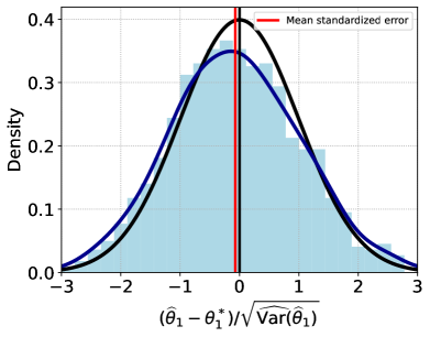
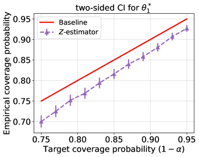
(a)		(b)

Figure 1: (a): Standardized estimation error of the $Z$-estimator (3b) for the first coordinate $\theta^{*}_{1}$; shown is a histogram based on $1000$ trials. (b): Empirical coverage probability of two-sided confidence interval for $\theta^{*}_{1}$ for a simulation for with parameters $(d_{T},d_{N},n)=(2,1000,950)$. See Section 4.1 for details.

In the definition (3a) of the score function $\psi_{i}$, the vector $p_{i}$ is the conditional mean of ${x}_{i}$ given the past data points. This $Z$-estimator is a classical method [50]; we refer readers to Section 2.1 and equation (36) for more details. When the data points are i.i.d., it can be shown [12] that ${\widetilde{\theta}}$ is $\sqrt{n}$-consistent and asymptotically normal.

A simple simulation reveals that these attractive guarantees can fail to hold under adaptive data collection. In particular, we performed experiments on a linear model (2) with $(d_{T},d_{N})=(2,1000)$, and in order to apply the LASSO bandit algorithm [46], we assumed that the nuisance vector ${\eta}\in{}^{1000}$ was $4$-sparse. We generated a path of $n=950$ samples using the LASSO bandit procedure to select the covariates in an adaptive fashion, as applied to the target vector $\theta^{*}=\begin{bmatrix}2&2\end{bmatrix}$.

Panel (a) of  Figure 1 shows that the standardized estimation error associated with $\widehat{\theta}_{1}$ is not standard Gaussian; instead, the distribution has a downward bias, as reflected by the negative mean $-0.07$ of the standardized errors. Thus, we see that asymptotic normality may fail to hold with adaptively collected data. Panel (b) of Figure 1 shows that confidence intervals constructed from the unweighted $Z$-estimator fail to provide the desired target coverage; in particular, the fraction of times that they cover the true parameter is consistently below the target coverage. This under-coverage is to be expected given the deviations of the standardized error from Gaussianity.

To be clear, such distributional anomalies are a wide-spread phenomenon: they are specific to neither the particular $Z$-estimator nor the LASSO bandit algorithm that we have simulated here. Similar types of breakdown are well-documented in the time series and forecasting literature, dating back to the classical work of Dickey and Fuller [17], White [60], and Lai and Wei [36]. More recent work [16, 64, 32] has highlighted a similar phenomenon in multi-armed bandit problems with popular selection algorithms like Thompson sampling, upper confidence bound (UCB), and $\epsilon$-greedy selection.

1.2 Related work

In this section, we survey existing literature on inference using adaptively collected data and semi-parametric inference that are relevant to our problem.

1.2.1 Inference using adaptively collected data

In their seminal work, Lai and Wei [36, 35] studied various regression models in which the covariate-response pairs are collected in an adaptive fashion. Among other results, they provided conditions under which the ordinary least squares (OLS) estimate is asymptotically normal. However, their results require a stability condition on the covariate matrix. This stability condition fails to hold in various settings, among them certain types of autoregressive models [17, 60, 36], the UCB and related online procedures for bandits [37], as well as offline procedures for multi-armed bandit problems with adaptively collected data (e.g., [16, 64]).

In order to address these challenges, Hadad et al. [23] proposed an adaptively weighted version of the augmented inverse propensity-weighted (AIPW, [40]) estimator for multi-armed bandits. They suggested certain choices of the adaptive weights that ensure the variance stabilization necessary to apply martingale central limit theory. Subsequent work by Zhan et al. [62] and Bibaut et al. [7] extend this approach to develop asymptotically normal estimators for contextual bandits. Zhang et al. [65] analyzes a weighted $M$-estimator for contextual bandit problems. Syrgkanis et al. [53] proposes a weighted $Z$-estimator for estimating the structural parameters in a structural mean nested model. All of these works on bandit problems all assume the data collection algorithm is known, and therefore enables the construction of weighted estimators based on the selection probability of each arm. Alternatively, when the bandit algorithm is unknown, Deshpande et al. [16] and Khamaru et al. [32] propose online-debiasing procedures that lead to asymptotically normal behavior.

1.2.2 Neyman orthogonality in semi-parametric inference

Semi-parametric statistics centers on how to estimate low-dimensional parameters in the presence of high-dimensional or nonparametric nuisance parameters, and is associated with a rich and evolving literature (e.g., [8, 48, 9, 50, 3, 49, 2, 56, 12]). A key concept is that of Neyman orthogonality [43] of the score function; it is a property that formalizes the first-order effect of perturbations in the nuisance terms on the target estimator. This notion has played an important role in semi-parametric estimation [3, 42]; targeted learning [56]; as well as inference for high-dimensional linear models [63, 5, 6, 28]. Sample splitting methods, in which different portions of the dataset are used to estimate the non-parametric and parametric components, are also commonly used in the literature (e.g., [8, 51, 18, 29]).

Chernozhukov et al. [12] combined the notion of Neyman orthogonality with sample splitting to construct $Z$-estimators that are asymptotically normal; they referred to this approach as double/debiased machine learning (DML). Sample splitting weakens the requirement of Donsker class conditions on the nuisance estimators, thereby allowing for the use of more sophisticated non-parametric procedures. Other procedures that build upon or are closely related to the DML approach have been developed for estimating heterogeneous treatment effects [44, 31, 19, 33, 52]; continuous treatment effects [14, 52]; tree-based methods [57, 4, 47]; statistical learning with nuisance parameters [22]; as well as dynamical treatment effects [38, 10, 13]. Some of this work goes beyond the i.i.d. setting in allowing for samples drawn from stable Markov chains, but do not address the general adaptive setting of interest in this paper.

In the i.i.d. setting, Belloni et al. [6] studied inference in generalized linear models with nuisance parameters, developing a general framework for inference of a one-dimensional parameter in the presence of high-dimensional nuisance. Liu et al. [39] propose an estimator for partially logistic regression models. Both works exploit Neyman orthogonality, and their methods involve solving a certain estimating equation, as in this paper. In this paper, we focus on a similar problem setting, but mainly as a vehicle to study the effect of adaptive data collection.

Non-asymptotic confidence intervals

As opposed to asymptotic guarantees, an alternative approach is to exploit concentration inequalities to construct non-asymptotic confidence regions that are valid uniformly in time. For instance, Abbasi et al. [1] prove an any-time self-normalized concentration inequality for bandit problems. These bounds were further developed for multi-armed bandits [27, 30] and for general sequential experiments [26]. On one hand, these methods are equipped with non-asymptotic guarantees, and remain relatively robust to model mis-specification. On the flip side, however, there are many settings in which these procedures lead to confidence intervals that are overly conservative relative to those constructed based on asymptotically normal estimators; for instance, see Figure 2 in the paper [23] for a comparison of this type.

1.3 Our contributions and paper organization

In this paper, we study how to estimate a target parameter $\theta^{*}$ associated with a generalized linear regression model in presence of both (possibly nonparametric) nuisance components, and a general model for adaptive data collection. Due to the sequential dependence induced by adaptive data collection, many standard $Z$-estimators may exhibit non-normal asymptotic behavior, and our main contribution is to rectify this issue. In order to do so, we propose and analyze a family of estimators for $\theta^{*}$ and show that under mild conditions these estimators are asymptotically unbiased and asymptotically normal. These procedures are based on an adaptive re-weighting of two-stage $Z$-estimators, so that we refer to them as AdapTZ methods. In 1, we discuss the AdapTZ-PL procedure that is tailored to the partial linear model, whereas 3 provides guarantees on a more general procedure (AdapTZ-GLM) that applies to generalized linear models. Under certain regularity conditions, both of these theorems yield an asymptotically valid confidence region for the parameter vector $\theta^{*}$. Next, we consider the problem of estimating a linear functional of the form $u^{\top}\theta^{*}$, where $u$ is any fixed unit vector in $\mathbb{R}^{d_{T}}$. In Theorems 2 and 4, we show that, for this simpler problem, it is possible to obtain asymptotic normality under much weaker conditions compared to Theorems 1 and 3. Finally, in Section 3, we demonstrate the usefulness of our general theory by developing its consequences for some concrete classes of semi-parametric models.

Notation:

For any numbers $n,n_{1},n_{2}\geq 1$ such that $n=n_{1}+n_{2}$ and a sequence of random variables $\{W_{i}\}_{i=1}^{n}$, we use the shorthand

$$\widehat{\mathbb{E}}_{n_{2}}f_{i}(W_{i})=\frac{1}{n_{2}}\sum_{i=n_{1}+1}^{n}f_{i}(W_{i})\quad\mbox{and}\quad\widetilde{\mathbb{E}}_{n_{2}}f_{i}(W_{i})=\frac{1}{n_{2}}\sum_{i=n_{1}+1}^{n}{\mathbb{E}}f_{i}(W_{i}\mid\mathcal{F}_{i-1})$$

We use $\|\cdot\|_{2}$ to denote the $2$-norm for a vector; for matrices, we use $|\mkern-2.0mu|\mkern-2.0mu|\cdot|\mkern-2.0mu|\mkern-2.0mu|_{{\mathrm{op}}}$ and $|\mkern-2.0mu|\mkern-2.0mu|\cdot|\mkern-2.0mu|\mkern-2.0mu|_{{F}}$ to denote their operator and Frobenius norms, respectively. For vectors $a,b\in{}^{d}$, we use $\langle a,\,b\rangle=\sum_{j=1}^{d}a_{j}b_{j}$ as a shorthand for their Euclidean inner product.

2 Main results

In this section, we first set up the class of problems to be studied in this paper. Our focus is asymptotic guarantees for the parameters of a generalized linear regression model in the presence of a non-parametric nuisance component. Our main results are analyses of two algorithms for estimation in the adaptive generalized model (4) with nuisance parameters. We derive several asymptotic normality guarantees on parameters of interest when these procedures are applied. Our first algorithm (AdapTZ-PL) is designed for the partial linear model (i.e., the special case $g(x)=x$), whereas the second one (AdapTZ-GLM) applies to more general non-linear link functions $g$.

2.1 Problem set-up

Suppose that a scalar response variable $y$ is linked to a covariate vector ${x}\in{}^{d_{T}}$ and auxiliary vector ${z}\in{}^{d_{N}}$ via the equation

$$y =g\big{(}\langle{x},\,\theta^{*}\rangle+h^{*}({z})\big{)}+\varepsilon,$$ (4)

where $\varepsilon$ is a zero-mean noise variable. Here $g:\real\rightarrow\real$ is a known link function, whereas $\theta^{*}\in\Theta\subset{}^{d_{T}}$ is an unknown target parameter, and the function $h^{*}:\mathbb{R}^{d_{N}}\rightarrow\mathbb{R}$ is also unknown. We assume that the target parameter space $\Theta$ is a bounded open subset of $\mathbb{R}^{d_{T}}$, whereas $h^{*}$ belongs to some class $\mathcal{H}$ of functions that are uniformly bounded in the supremum norm.

The model (4) is a particular instantiation of a semi-parametric model, as it contains both a parametric and a non-parametric component. Of primary interest is the parametric component $\theta^{*}$: our goal is to develop point estimates as well as confidence sets associated with these estimates. In this context, the unknown function $h^{*}$ plays the role of a nuisance parameter. It needs to be controlled to obtain a good estimate of $\theta^{*}$, but is not of intrinsic interest in its own right.

2.1.1 Allowed forms of adaptive data collection

In order to estimate the target parameter $\theta^{*}$, we observe a collection of $n$ samples, each of the form $({x}_{i},y_{i},{z}_{i})$ for $i=1,\ldots,n$. We allow the data collection to be sequentially dependent in the following way. The samples define a nested sequence of $\sigma$-fields with $\mathcal{F}_{0}=\emptyset$, and

$$\mathcal{F}_{i-1} =\sigma\Big{(}\{{x}_{j},y_{j},{z}_{j}\}_{j=1}^{i-1}\Big{)}\qquad\mbox{for each $i=2,\ldots,n$.}$$ (5)

Let $\mathcal{P}$ be a family of distributions on $\mathbb{R}^{d_{N}}$. At stage $i=1,\ldots,n$, we assume that:

• the distribution of the nuisance vector ${z}_{i}$ conditioned on $\mathcal{F}_{i-1}$ belongs to $\mathcal{P}$.

• the choice of regressor ${x}_{i}$ is determined according to a known selection function that maps pairs $({z}_{i},\mathcal{F}_{i-1})$ to probabilities $p_{i}({z}_{i},\mathcal{F}_{i-1})\in[0,1]$.

With a slight abuse of notation, we often adopt the shorthand $p_{i}$ for the function value $p_{i}({z}_{i},\mathcal{F}_{i-1})$. Throughout this paper, we assume that the selection functions are known to us; for example, these functions could correspond to policies in the setting of a contextual bandit.

Structural assumptions:

Our analysis involves some structural assumptions on the link function $g$, as well as the space $\mathcal{X}\subset{}^{d_{T}}$ in which the covariates lie.

• In 1 and 2, we provide guarantees for $g(x)=x$, in which case our general set-up (4) reduces to the setting of partial linear regression.

• In 3 and 4, we allow the function $g$ to be non-linear, requiring only certain smoothness and identifiability conditions.

• Throughout the paper, we assume that the $d_{T}$-dimensional regressor vector ${x}$ takes values in a discrete set that consists of an orthonormal basis of ${}^{d_{T}}$, along with the all-zeros vector. Without loss of generality—rotating as needed—we can assume that the orthonormal basis is the standard one $\{e_{1},\ldots,e_{d_{T}}\}$, where $e_{j}\in{}^{d_{T}}$ is the vector with a single one in coordinate $j$ (and zeros elsewhere). This particular setting arises naturally for multi-armed bandits and treatment assignment problems.

Given the assumed structure of the covariates, the selection functions are naturally viewed as selection probabilities—that is, for each $i=1,\ldots,n$ and $j=1,\ldots,d_{T}$

$$p_{ij} :=\mathbb{E}\big{[}{x}_{ij}\mid\mathcal{F}_{i-1},{z}_{i}\big{]}$$ (6)

is the conditional probability that ${x}_{i}=e_{j}$. Thus, the conditional probability of ${x}_{i}=0$ is given by $p_{i0}:=1-\sum_{j=1}^{d_{T}}p_{ij}$.

2.2 Guarantees for the partial linear model

This section is devoted to a special case of the general set-up: choosing $g({x})={x}$ leads to the partial linear regression model

$$y_{i} =\langle{x}_{i},\,\theta^{*}\rangle+h^{*}({z}_{i})+\varepsilon_{i}.$$ (7)

We assume that the target parameter $\theta^{*}$ lies in a bounded open subset $\Theta\subset{}^{d_{T}}$, whereas the nuisance function $h^{*}$ belongs to a function class $\mathcal{H}$ with bounded $\ell_{\infty}$-norm.

2.2.1 Estimating the target parameter $\theta^{*}$

Our procedure is a particular type of $Z$-estimator, in that we compute the solution to a set of equations based on a $d_{T}$-dimensional score function. Let us introduce some notation required to define this score function. The conditional covariance of the regression vector ${x}_{i}$, when conditioned upon the pair $(\mathcal{F}_{i-1},{z}_{i})$, is given by

$${\mathbf{\Sigma}}_{i} :=\mathbb{E}\big{[}({x}_{i}-p_{i})({x}_{i}-p_{i})^{\top}\mid\mathcal{F}_{i-1},{z}_{i}\big{]},$$ (8)

where $p\in{}^{d_{T}}$ is the vector of selection probabilities previously defined. Note that this matrix can be computed at each time $i$, since it is assumed that we know the selection mechanism. Using this random matrix, we then construct the score function

$$\phi_{i}(\theta,h) :={\mathbf{\Sigma}}_{i}^{-1/2}({x}_{i}-p_{i})\big{\{}y_{i}-\langle{x}_{i},\,\theta\rangle-h({z}_{i})\big{\}},$$ (9)

Strictly speaking, this score function $\phi_{i}$ also depends on the quadruple $(y_{i},{x}_{i},{z}_{i},\mathcal{F}_{i-1})$, but we omit this dependence for notational simplicity. An important property of $\phi_{i}$ is that it is conditionally mean zero—viz.

$$\mathbb{E}\big{[}\phi_{i}(\theta^{*},h^{*})\mid\mathcal{F}_{i-1}\big{]} =0.$$ (10a)

Moreover, it satisfies the Neyman orthogonality condition,

$$\mathbb{E}\big{[}\partial_{h}\phi_{i}(\theta^{*},h^{*})\{h-h^{*}\}\mid\mathcal{F}_{i-1}\big{]} =0\qquad\mbox{for any $h\in\mathcal{H}$,}$$ (10b)

where $\partial_{h}\phi_{i}$ is the Gateaux derivative. See Appendix B for more details on this derivative and orthogonality condition.

The conditional mean property (10a) is needed to ensure consistency at the population level, whereas the Neyman condition (10b) guarantees that, again at the population level, the first-order effect of perturbing the nuisance parameter vanishes. With this intuition in place, we state our procedure formally as Algorithm 1, and refer to it for short as AdapTZ-PL, or adaptive two-stage $Z$-estimation for the partially linear model.

Algorithm 1       AdapTZ-PL: partial linear model

1:  Given $n$ samples $\big{\{}({x}_{i},{z}_{i},y_{i})\big{\}}_{i=1}^{n}$ from the partial linear model (7).

2:  Define the index sets $I_{1}:=\{1,2,\ldots,n_{1}\}$ and $I_{2}:=\{n_{1}+1,\ldots,n\}$, and set $n_{2}:=n-n_{1}$.

3:   Compute an estimate $\widehat{h}$ of the nuisance function $h^{*}$ based on the samples $\{(y_{i},{x}_{i},{z}_{i})\}_{i\in I_{1}}$.

4:  Based on the samples $\{(y_{i},{x}_{i},{z}_{i})\}_{i\in I_{2}}$, form the estimating equations

$$\frac{1}{n_{2}}\sum\limits_{i\in I_{2}}\phi_{i}(\theta,\widehat{h}) =0,$$ (11)

and compute a solution ${\widetilde{\theta}}$.

Note: By the definition (9) of the score functions $\phi_{i}$, the estimating equations (11) are linear in the parameter $\theta$; moreover, our analysis in proving 1 establishes that this linear system has a unique solution ${\widetilde{\theta}}$ with probability tending to one as $n$ increases.

2.2.2 Asymptotic normality

The main result of this section is an asymptotic normality guarantee for the vector ${\widetilde{\theta}}$ computed using the AdapTZ-PL algorithm. We begin by stating our assumptions and discussing their role in the theorem.

1. Conditioned upon $({x}_{i},{z}_{i},\mathcal{F}_{i-1})$, each element of the zero-mean noise sequence $\{\varepsilon_{i}\}_{i=1}^{n}$ is sub-Gaussian with parameter $\nu$, and has conditional variance ${\sigma^{2}:=\mathbb{E}[\varepsilon_{i}^{2}\mid{x}_{i},{z}_{i},\mathcal{F}_{i-1}]}$.

1. The selection probabilities $p_{ij}$ at each round $i$ satisfy the lower bound

   $$p_{ij} \geq\frac{c_{0}}{i^{2t}}\quad\mbox{for all $j=0,1,\ldots,d_{T}$ and $i=1,2,\ldots$,}$$ (12)

   for some constant $c_{0}>0$ and exponent $t\in[0,\tfrac{1}{2})$.

1. Let $\mathcal{P}$ be a family of distributions sufficiently rich to contain all possible distributions of ${z}_{i}$ conditioned on $\mathcal{F}_{i-1}$, for all $i\geq 1$. The estimator $\widehat{h}$ obtained from Step 3 of the AdapTZ-PL procedure satisfies

   $$\sup_{P\in\mathcal{P}}(\mathbb{E}_{v\sim P}|\widehat{h}(v)-h^{*}(v)|^{2})^{1/2}=o_{p}(1).$$ (13)

Let us clarify the meaning and significance of these assumptions. The noise condition (NOI$(\nu,\sigma^{2})$)10pt allows us to control the tail behavior of the noise, and is relatively standard. More interesting is the selection condition (SEL$(t)$)10pt, which allows the minimum selection probability to decrease as fast as $n^{-2t}$ for some $t\in[0,1/2)$. This is substantially weaker than assumptions used in past work, such as requiring that the selection probabilities be uniformly bounded away from zero [65]; or converge to some non-random limit [23, 62]. Finally, the nuisance condition (NUI)10pt guarantees that the estimate $\widehat{h}$ based on the hold-out set is a weakly-consistent estimator for the true nuisance function $h^{*}$.

With this set-up, we now state our first main result:

Theorem 1.

Suppose that Assumptions (NOI$(\nu,\sigma^{2})$)10pt,  (SEL$(t)$)10pt and (NUI)10pt are in force. Then the estimate ${\widetilde{\theta}}$ obtained from AdapTZ-PL (Algorithm 1) satisfies

$$(\sqrt{n_{2}}\widehat{\mathbb{E}}_{n_{2}}{\mathbf{\Sigma}}_{i}^{1/2})({\widetilde{\theta}}-\theta^{*}) \stackrel{{\scriptstyle d}}{{\rightarrow}}\mathcal{N}(0,\sigma^{2}\mathbf{I}_{d_{T}}).$$ (14)

See Section 5.1 for the proof.

A few comments regarding this claim are in order.

IID nuisance:

Finding a suitable choice of $\mathcal{P}$ for verifying the condition (13) is non-trivial in general. However, when the nuisances ${z}_{i}$ are i.i.d. and independent of $\mathcal{F}_{i-1}$, this condition reduces to $(\mathbb{E}|\widehat{h}({z}_{i})-h^{*}({z}_{i})|^{2})^{1/2}=o_{p}(1)$, and so is concrete and explicit.

Linear nuisance function:

Suppose that the nuisance function is linear in ${z}$—that is, say ${h^{*}({z})=\langle{z},\,{\eta}^{*}\rangle}$ for some ${\eta}^{*}\in\mathbb{R}^{d_{N}}$—and that $\mathbb{E}\|{z}_{i}\|_{2}^{2}\leq M_{z}<\infty$ for all $i\geq 1$. Under these conditions, given an estimate ${\widehat{{\eta}}}$ with $\|{\widehat{{\eta}}}-{\eta}^{*}\|_{2}=o_{p}(1)$, it follows that Assumption (NUI)10pt holds with $\widehat{h}({z})=\langle{z},\,{\widehat{{\eta}}}\rangle$, and $\mathcal{P}$ given by the set of all distributions with second moment at most $M_{z}$.

Generalization to arbitrary orthonormal basis:

In 1, we assumed that the regressors ${x}_{i}$ takes one of the $d_{T}+1$ values $\{e_{1},\ldots,e_{d_{T}}\}\cup 0$. However, as remarked earlier, conditioned on assuming that the covariates are orthogonal, assuming this canonical basis actually entails no loss of generality. More precisely, a simple calculation shows that we can replace $\{e_{1},\ldots,e_{d_{T}}\}$ with any orthonormal basis $\{u_{1},\ldots,u_{d_{T}}\}$ in $\mathbb{R}^{d_{T}}$. In this case, the rotated matrix variant of 1 holds with $\Sigma_{i}$ replaced by

$$\operatorname{Cov}({x}_{i}\mid\mathcal{F}_{i-1},{z}_{i}) =\mathbf{U}\mathbf{\Sigma}_{i}(\mathcal{F}_{i-1},{z}_{i})\mathbf{U}^{\top},$$

where $\mathbf{U}\equiv(u_{1},\ldots,u_{d_{T}})$. Consequently, we have

$$\big{\{}\sqrt{n_{2}}\mathbf{U}\widehat{\mathbb{E}}_{n_{2}}{\mathbf{\Sigma}}_{i}^{1/2}\mathbf{U}^{\top}\big{\}}({\widetilde{\theta}}-\theta^{*})\stackrel{{\scriptstyle d}}{{\rightarrow}}\mathcal{N}(0,\sigma^{2}\mathbf{I}_{d_{T}}).$$

Computational complexity:

Note that the matrix ${\mathbf{\Sigma}}_{i}$ is the covariance of a multinomial distribution, and a Cholesky decomposition of such matrices can be carried out in $\mathcal{O}(d_{T}^{2})$ time. Therefore, the time complexity of setting up the estimating equations (11) scales $\mathcal{O}(nd_{T}^{2})$. Solving the system of linear equations requires at most $\mathcal{O}(d_{T}^{2})$ time.

Inference for the target parameter:

From 1, we can construct a confidence region for the whole parameter vector (e.g., by a $\chi^{2}$-test). In addition, if the sequence of random matrices $\widehat{\mathbb{E}}_{n_{2}}[{\mathbf{\Sigma}}_{i}^{1/2}]$ converge to some non-random and invertible matrix—say $\mathbf{\Gamma}^{1/2}$—then equation (14) implies that $\sqrt{n_{2}}({\widehat{\theta}}-\theta^{*})$ is asymptotically normal with covariance $\mathbf{\Gamma}^{-1}$.

2.3 Fixed direction inference for the partial linear model

In various applications, one is only interested in estimating linear functionals of the target parameter vector. Concretely, given a unit-norm vector $u\in\mathbb{R}^{d_{T}}$, consider the problem of providing confidence intervals for the scalar target $\theta^{*}_{u}:=\langle u,\,\theta^{*}\rangle$; standard examples include the first coordinate $\theta^{*}_{1}$, or the difference between two coordinates $\theta^{*}_{1}-\theta^{*}_{2}$. In this section, we show that inferential guarantees for such scalar quantities can be obtained under much weaker conditions than 1. Namely, we only require Assumption (SEL$(t)$)10pt to hold for coordinates $j$ for which $u_{j}$ is non-zero.

2.3.1 Constructing the score function

Suppose that we compute an initial pair of “crude” estimates ${\widehat{\theta}}$ and $\widehat{h}$ using the dataset $\big{\{}({x}_{i},{z}_{i},y_{i})\big{\}}_{i=1}^{n_{1}}$. Recalling that $\langle\cdot,\,\cdot\rangle$ denotes the Euclidean inner product, we consider the one-dimensional score function

$$\phi_{i1}(\theta_{u},{\widehat{\theta}},\widehat{h})=\langle A_{i1},\,{x}_{i}-p_{i}\rangle\big{\{}y_{i}-\langle{x}_{i},\,u\rangle\theta_{u}-{x}_{i}^{\top}(\mathbf{I}_{d_{T}}-uu^{\top}){\widehat{\theta}}-\widehat{h}({z}_{i})\big{\}},$$ (15a)

where the vector $$A_{i1}$$ is defined as

$$A_{i1}=\big{(}\mathbf{\Sigma}_{i}^{-1}u\big{)}\tfrac{1}{\sqrt{u^{\top}{\mathbf{\Sigma}^{-1}_{i}}u}},$$

and the inverse covariance matrix $${\mathbf{\Sigma}}_{i}^{-1}$$ admits the explicit expression

$${\mathbf{\Sigma}}_{i}^{-1}({z}_{i},\mathcal{F}_{i-1}) =\begin{pmatrix}\frac{1}{p_{i1}}+\gamma_{i}&\gamma_{i}&\gamma_{i}&\cdots&\gamma_{i}\\ \gamma_{i}&\frac{1}{p_{i2}}+\gamma_{i}&\gamma_{i}&\cdots&\gamma_{i}\\ \gamma_{i}&\gamma_{i}&\frac{1}{p_{i3}}+\gamma_{i}&\cdots&\gamma_{i}\\ \vdots&\vdots&\vdots&\vdots&\vdots\\ \gamma_{i}&\gamma_{i}&\cdots&\gamma_{i}&\frac{1}{p_{id_{T}}}+\gamma_{i}\end{pmatrix},$$ (15b)

where $$\gamma_{i}=1/p_{i0} A_{i1} \mathbb{E}|\langle A_{i1},\,{x}_{i}-p_{i}\rangle|^{2}=1 {\widetilde{\theta}}_{u}$$. With this choice of , we can stabilize the variance of the score function, namely, we have . Next, we find by solving the linear system

$$\frac{1}{n_{2}}\sum_{i=n_{1}+1}^{n_{2}}\phi_{i1}({\widetilde{\theta}}_{u},{\widehat{\theta}},\widehat{h})=0$$ (15c)

2.3.2 Guarantee of asymptotic normality

We are now ready to establish a guarantee for the estimate $\theta^{*}_{u}$. We do so under the following weaker variant of our earlier selection condition (SEL$(t)$)10pt:

1. For some $t\in[0,\tfrac{1}{2})$, the selection probabilities are lower bounded as

   $$p_{ij}\succeq\frac{c_{0}}{i^{2t}}\quad\mbox{for all $j\in S_{u}\cup\{0\}$, and for all $i=1,2\ldots$,}$$ (16)

   where $S_{u}:=\{j\mid u_{j}\neq 0\}$ is the support set of $u$.

Compared to our earlier selection condition (SEL$(t)$)10pt, Assumption (SEL${}^{\ast}(t,u,S_{u})$)10pt is weaker in the sense that the lower bound condition is imposed only on the support set of the vector $u$, along with the reference point (the all-zeroes vector). This difference is significant, for example, when our goal is to estimate a single coordinate, or the difference of two coordinates.

Theorem 2.

Suppose that Assumptions (NOI$(\nu,\sigma^{2})$)10pt,  (SEL${}^{\ast}(t,u,S_{u})$)10pt and (NUI)10pt are in force. Then the $Z$-estimate ${\widetilde{\theta}}_{u}$ computed from (15c) using any consistent estimate ${\widehat{\theta}}$ of $\theta$ satisfies

$$\Big{(}\widehat{\mathbb{E}}_{n_{2}}\tfrac{1}{\sqrt{u^{\top}{\mathbf{\Sigma}}_{i}^{-1}u}}\Big{)}({\widetilde{\theta}}_{u}-\theta^{*}_{u})\stackrel{{\scriptstyle d}}{{\rightarrow}}\mathcal{N}(0,\sigma^{2}).$$

See Section 5.2 for the proof.

A few comments regrading 2 are in order. First, its guarantees hold under a weaker assumption on the selection probability, albeit at the expense of assuming the a priori existence of a consistent estimator of ${\widehat{\theta}}$. However, since typically we estimate $\theta^{*},h^{*}$ simultaneously in the partial linear model, we would also obtain a consistent estimator of $\theta^{*}$ if we can find a consistent estimator of $h^{*}$ (cf. condition (13)).

Second, suppose that the nuisance function is linear—i.e., $h^{*}({z})=\langle{z},\,{\eta}^{*}\rangle$ for some ${\eta}^{*}\in\mathbb{R}^{d_{N}}$. Similar to 1, let ${\widehat{{\eta}}}$ be an estimator of ${\eta}^{*}$ with $\|{\widehat{{\eta}}}-{\eta}^{*}\|_{2}=o_{p}(1)$ and assume that $\sup_{i}\mathbb{E}\|{z}_{i}\|_{2}^{2}\leq M_{z}<\infty$, then Assumption (NUI)10pt is satisfied with $\widehat{h}({z})=\langle{z},\,{\widehat{{\eta}}}\rangle$ and $\mathcal{P}$ be the set of distributions with the second moment less than $M_{z}$.

Observe that 2 allows us to construct an asymptotically valid level-$\alpha$ confidence interval for $\theta^{*}_{u}$. Specifically, we have

$$\lim_{n\to\infty}{\mathbb{P}}\left[{\widetilde{\theta}}_{u}-\tfrac{q_{1-\alpha/2}\sigma}{\sqrt{n_{2}}}\Big{(}\widehat{\mathbb{E}}_{n_{2}}\tfrac{1}{\sqrt{u^{\top}{\mathbf{\Sigma}}_{i}^{-1}u}}\Big{)}^{-1}\leq\theta^{*}_{u}\leq{\widetilde{\theta}}_{u}+\tfrac{q_{1-\alpha/2}\sigma}{\sqrt{n_{2}}}\Big{(}\widehat{\mathbb{E}}_{n_{2}}\tfrac{1}{\sqrt{u^{\top}{\mathbf{\Sigma}}_{i}^{-1}u}}\Big{)}^{-1}\right]=1-\alpha,$$

where $q_{1-\alpha/2}$ is the $1-\alpha/2$ quantile of standard normal distribution. In particular, if we are interested in the first co-ordinate $\theta^{*}_{1}$, then setting $u=e_{1}$ and applying 2 yields

$$\Big{(}\widehat{\mathbb{E}}_{n_{2}}\sqrt{\frac{p_{i0}p_{i1}}{p_{i0}+p_{i1}}}\Big{)}({\widetilde{\theta}}_{1}-\theta^{*}_{1})\stackrel{{\scriptstyle d}}{{\rightarrow}}\mathcal{N}(0,\sigma^{2}).$$

Third, although we have stated the result with ${\widehat{\theta}}$ assumed to be consistent for the full vector $\theta$, in fact, we require only that that is consistent for any direction that is orthogonal to $u$, i.e., it suffices to have the slightly weaker consistency condition $(\mathbf{I}_{d_{T}}-uu^{\top})({\widehat{\theta}}-\theta^{*})\overset{p}{\to}0$.

2.4 Generalized linear model

We now return to the general setting, in which we have a model of the form

$$y_{i} =g\big{(}\langle{x}_{i},\,\theta^{*}\rangle+h^{*}({z}_{i})\big{)}+\varepsilon_{i},$$ (17)

for a general choice of inverse link $g$. We assume that the parameter $(\theta^{*},h^{*})\in\Theta\times\mathcal{H}$, where the parameter space $\Theta$ is a bounded open set in $\mathbb{R}^{d_{T}}$ and $\mathcal{H}$ is a set of functions with bounded $\ell_{\infty}$-norm.

2.4.1 Estimating the target parameter $\theta^{*}$

We start by constructing a different score function. Namely, we introduce an auxiliary nuisance vector ${\makebox[0.0pt][l]{\hskip 2.08334pt\rule[8.23611pt]{2.48053pt}{0.43057pt}}{\theta}}$ and define

$$\phi_{i}(\theta,{\makebox[0.0pt][l]{\hskip 2.08334pt\rule[8.23611pt]{2.48053pt}{0.43057pt}}{\theta}},h)\equiv\mathbf{\Omega}_{i}({x}_{i}-m_{i})\;\Big{\{}y_{i}-g\big{(}\langle{x}_{i},\,\theta\rangle+h({z}_{i})\big{)}\Big{\}}$$ (18)

where

$$m_{i} \equiv\mathbb{E}(({x}_{i}g^{\prime}\big{(}\langle{x}_{i},\,{\makebox[0.0pt][l]{\hskip 2.08334pt\rule[8.23611pt]{2.48053pt}{0.43057pt}}{\theta}}\rangle+h({z}_{i})\big{)}|{z}_{i},\mathcal{F}_{i-1})[\mathbb{E}(g^{\prime}\big{(}\langle{x}_{i},\,{\makebox[0.0pt][l]{\hskip 2.08334pt\rule[8.23611pt]{2.48053pt}{0.43057pt}}{\theta}}\rangle+h({z}_{i})\big{)}|{z}_{i},\mathcal{F}_{i-1})]^{-1},$$ (19a)

$$\mathbf{\Omega}_{i} \equiv{}[\mathbb{E}(\varepsilon_{i}^{2}({x}_{i}-m_{i})({x}_{i}-m_{i})^{\top}|{z}_{i},\mathcal{F}_{i-1})]^{-1/2}$$

$$=[\mathbb{E}(\mathcal{E}^{2}\big{(}g\big{(}\langle{x}_{i},\,{\makebox[0.0pt][l]{\hskip 2.08334pt\rule[8.23611pt]{2.48053pt}{0.43057pt}}{\theta}}\rangle+h({z}_{i})\big{)}\big{)}({x}_{i}-m_{i})({x}_{i}-m_{i})^{\top}|{z}_{i},\mathcal{F}_{i-1})]^{-1/2}$$ (19b)

and $\mathcal{E}^{2}(x)\equiv\mathbb{E}(\varepsilon_{i}^{2}|g\big{(}\langle{x}_{i},\,\theta^{*}\rangle+h^{*}({z}_{i})\big{)}=x)$ is the conditional variance of the noise $\varepsilon_{i}$. When ${\makebox[0.0pt][l]{\hskip 2.08334pt\rule[8.23611pt]{2.48053pt}{0.43057pt}}{\theta}}=\theta^{*}(\text{or\,}{\widehat{\theta}})$ and $h=h^{*}(\text{or\,}\widehat{h})$, we denote the corresponding $m_{i}$ and $\mathbf{\Omega}_{i}$ by $m^{*}_{i}~{}(\text{or\,}\widehat{m}_{i})$ and $\mathbf{\Omega}^{*}_{i}~{}(\text{or\,}\widehat{}\mathbf{\Omega}_{i})$ respectively. Intuitively speaking, the vector $m_{i}$ can be viewed as a weighted conditional expectation of the regressor ${x}_{i}$, while the matrix $\mathbf{\Omega}_{i}$ can be viewed the inverse square root of a weighted conditional covariance matrix of ${x}_{i}$. When $g(x)=x$, $m,\mathbf{\Omega}$ does not depend on ${\makebox[0.0pt][l]{\hskip 2.08334pt\rule[8.23611pt]{2.48053pt}{0.43057pt}}{\theta}}$ and the score function in equation (18) reduces to the early one in equation (9) for the partial linear model.

Similar to the partial linear model case, this score function satisfies a version of the Neyman orthogonality condition. Namely,

$$\mathbb{E}(\phi(\theta^{*},\theta^{*},h^{*})|\mathcal{F}_{i-1}) =0,$$ (20a)

$$\mathbb{E}(\partial_{{\makebox[0.0pt][l]{\hskip 1.45834pt\rule[5.76527pt]{1.73636pt}{0.3014pt}}{\theta}}}\phi_{i}(\theta^{*},\theta^{*},h^{*})|\mathcal{F}_{i-1}) =0,\text{and}$$ (20b)

$$\mathbb{E}(\partial_{h}\phi_{i}(\theta^{*},\theta^{*},h^{*})[h-h^{*}]|\mathcal{F}_{i-1}) =0\text{~{}~{}for all~{}~{}}h\in\mathcal{H}.$$ (20c)

We defer the proof of these equations to Appendix B. Now, we estimate the target parameter $\theta^{*}$ using the following AdapTZ-GLM procedure, or adaptive two-stage $Z$-estimation for the generalized linear model.

Algorithm 2       AdapTZ-GLM: generalized linear model

1:  Given $n$ samples $\big{\{}({x}_{i},{z}_{i},y_{i})\big{\}}_{i=1}^{n}$ from the partial linear model (17).

2:  Define the index sets $I_{1}:=\{1,2,\ldots,n_{1}\}$ and $I_{2}:=\{n_{1}+1,\ldots,n\}$, and define $n_{2}=n-n_{1}$.

3:  Use samples $\{(y_{i},{x}_{i},{z}_{i})_{i\in I_{1}}\}$ to obtain an estimate $\widehat{h}$ for the nuisance function $h^{*}$ and ${\widehat{\theta}}$ for the target parameter $\theta^{*}$.

4:  Find ${\widetilde{\theta}}$ by solving the equation

$$\frac{1}{n_{2}}\sum\limits_{i\in I_{2}}\phi_{i}({\widetilde{\theta}},{\widehat{\theta}},\widehat{h})=0$$ (21)

.

2.4.2 Asymptotic normality

We now turn to a result on the asymptotic normality of the estimator ${\widetilde{\theta}}$ computed using the AdapTZ-GLM procedure described as Algorithm 2. Let us begin with the underlying assumptions.

1. For some $t\in[0,\tfrac{1}{4}]$ and $\delta>0$, the selection probabilities $p_{ik}$ are lower bounded as

   $$p_{ik}\geq c_{i}:=\frac{c_{0}}{i^{2(t-\delta)}}\quad\mbox{for all $k=1,\ldots,d_{T}$, and $i=1,2,\ldots$.}$$ (22)

   In addition, the probability of selecting the zero vector satisfies $p_{i0}\geq\tilde{c}_{0}$ for some $\tilde{c}_{0}>0$.

1. Suppose that all distributions in $\mathcal{P}$ are supported on a set $\mathrm{dom}(\mathcal{P})$ (can be $\mathbb{R}^{d_{N}}$). The estimators ${\widehat{\theta}},\widehat{h}$ obtained in Step 3 of Algorithm 2 satisfy $\|{\widehat{\theta}}-\theta^{*}\|_{2}=o_{p}(n^{-1/4})$, and $\sup\limits_{v\in\mathrm{dom}(\mathcal{P})}|\widehat{h}(v)-h^{*}(v)|=o_{p}(n^{-1/4})$.

1. The model is identifiable under our choice of the score function, concretely,

   $$\|\widetilde{\mathbb{E}}_{n_{2}}(\phi_{i}(\theta,\theta^{*},h^{*})-\phi_{i}(\theta^{*},\theta^{*},h^{*}))\|_{2} \geq\frac{1}{2}\|\widetilde{\mathbb{E}}_{n_{2}}\partial_{\theta}\phi_{i}(\theta^{*},\theta^{*},h^{*})(\theta-\theta^{*})\|_{2}\wedge c_{\phi}n^{-1/4}$$

   almost surely for any $\theta\in\mathbb{R}^{d_{T}}$ and some constant $c_{\phi}>0$ .

1. The minimum singular value of the gradient $\widetilde{\mathbb{E}}_{n_{2}}\partial_{\theta}\phi_{i}(y_{i},{x}_{i},{z}_{i},\mathcal{F}_{i-1},\theta^{*},\theta^{*},h^{*})$ is not too small, namely,

   $$\lim_{n\to\infty}{\mathbb{P}}(\sigma_{\min}(\widetilde{\mathbb{E}}_{n_{2}}\mathbf{\Omega}^{*}_{i}({x}_{i}-m^{*}_{i})g^{\prime}\big{(}\langle{x}_{i},\,\theta^{*}\rangle+h^{*}({z}_{i})\big{)}({x}_{i}-m^{*}_{i})^{\top})\geq m_{\phi}n^{\delta-t}) \to 1$$

   for some constant $m_{\phi}>0$.

2.4.3 Other standard GLM assumptions:

In addition to the above four assumptions, we make the additional assumptions on our generalized linear model.

• There exist constants $M_{\theta}$ and $D_{x}>0$ such that $\sup_{\theta\in\Theta}\|\theta\|_{2}\leq M_{\theta}$, $\|{x}_{i}\|_{2}\leq D_{x}$, and $h^{*}$ satisfies $\|h^{*}({z}_{i})\|_{\infty}\leq M_{h}$ for some $M_{h}>0$.

• The conditional variance $\mathcal{E}^{2}(x)$ is three-times differentiable, $\mathcal{E}^{2}(x),\mathcal{E}^{2^{\prime}}(x)$ are $L_{\varepsilon},L_{\varepsilon^{\prime}}$-Lipschitz respectively for $|x|\leq M_{h}+D_{x}M_{\theta}$, and there exist some $M_{\varepsilon},m_{\varepsilon}>0$ such that $M_{\varepsilon}\geq\mathcal{E}^{2}(x)\geq m_{\varepsilon}$ for $|x|\leq M_{h}+D_{x}M_{\theta}$. Furthermore, we assume that the zero mean noise $\varepsilon_{i}$ is sub-Gaussian with parameter $\nu$ conditioned ${x}_{i},{z}_{i},\mathcal{F}_{i-1}$.

• The inverse link function $g$ is three-times differentiable, monotone and the functions $g,g^{\prime},g^{{}^{\prime\prime}}$ are $L_{g},L_{g^{\prime}},L_{g^{{}^{\prime\prime}}}$-Lipschitz continuous, respectively. Moreover,
  $\inf_{|x|\leq M_{h}+D_{x}M_{\theta}}|g^{\prime}(x)|\geq l_{g}$ for some $l_{g}>0$.

Assumption (SEL${}^{\prime}(t,\delta)$)10pt is slightly stronger than Assumption (SEL$(t)$)10pt in the sense that we need to replace $t$ by $t-\delta$ for some small constant $\delta$ and restrict $t\in[0,1/4]$. Assumption (NUI^′)10pt is made on the performance of the pilot estimators. The reason we assume ${\widehat{\theta}}-\theta^{*}=o_{p}(n^{-1/4})$ is to ensure second order terms in the Taylor expansion of the score function vanish.

The conditions (IDE)10pt and (EIG)10pt ensure that the expectation of score function is sufficiently away from zero when $\theta$ is away from $\theta^{*}$. In the simple scenario where $g(x)=x$, Assumption (IDE)10pt and (EIG)10pt are implied by the rest assumptions. Also, it can be shown that Assumption (EIG)10pt holds in logistic regression (see Section D.3 for detailed derivations). However, due to the adaptive nature of the collected data, it is in general hard to verify these two assumptions. To address this issue, in practice, we suggest verifying them with all $\widetilde{\mathbb{E}}_{n_{2}}$ replaced by $\widehat{\mathbb{E}}_{n_{2}}$ instead. Since the empirical mean concentrates around the conditional expectation, the empirical version of Assumption (IDE)10pt and (EIG)10pt hold with high probability when the assumptions themselves are true. Therefore, we may use the empirical version as a surrogate for the original assumptions.

Finally, in Section 2.4.3 we enlist some standard assumptions on the GLM. The first condition assumes boundedness condition in the regressors, the parameter space, and the true nonlinear function. The second and third condition respectively puts some smoothness condition on the conditional variance functional $\mathcal{E}^{2}(\cdot)$ and the link function g.

Theorem 3.

Suppose that Assumptions (SEL${}^{\prime}(t,\delta)$)10pt—(EIG)10pt and the standard GLM assumptions from Section 2.4.3 are in force. Then the estimate ${\widetilde{\theta}}$ obtained from AdapTZ-GLM (cf. Algorithm 2) satisfies

$$(\widehat{\mathbb{E}}_{n_{2}}\widehat{}\mathbf{\Omega}_{i}({x}_{i}-\widehat{m}_{i})g^{\prime}\big{(}\langle{x}_{i},\,{\widehat{\theta}}\rangle+\widehat{h}({z}_{i})\big{)}({x}_{i}-\widehat{m}_{i})^{\top})\sqrt{n_{2}}({\widetilde{\theta}}-\theta^{*})\stackrel{{\scriptstyle d}}{{\rightarrow}}\mathcal{N}(0,\mathbf{I}_{d_{T}}).$$ (23)

See Section 5.3 for the proof.

A simple case is when the nuisance function is linear, i.e., $h^{*}({z})=\langle{z},\,{\eta}^{*}\rangle$ for some ${\eta}^{*}\in{\eta}$, and $\mathcal{H}$ is a bounded set in $\mathbb{R}^{d_{N}}$. In this case, the assumptions from Section 2.4.3 hold if there exist $M_{{\eta}},D_{x}>0$ such that $\sup_{{\eta}\in\mathcal{H}}\|{\eta}\|_{2}\leq M_{{\eta}}$ and $\|({x}_{i}^{\top},{z}_{i}^{\top})^{\top}\|_{2}\leq D_{x}$. Moreover, Assumption (NUI^′)10pt is satisfied if in addition we have an estimator ${\widehat{{\eta}}}\in\mathcal{H}$ such that $\|{\widehat{{\eta}}}-{\eta}^{*}\|_{2}=o_{p}(n^{-1/4})$.

Similar to the partial linear model discussed in Section 2.2,  3 allows us to construct a confidence region for the parameter vector $\theta^{*}$ via a $\chi^{2}-$ test. Also, if the weighted matrix on the L.H.S. of equation (23) converges, then $\sqrt{n_{2}}({\widetilde{\theta}}-\theta^{*})$ is asymptotically normal, and we can construct a confidence region (interval) for any subset of the parameter vector $\theta^{*}$. In absence of such convergence, we cannot obtain a confidence interval for fixed directions of $\theta^{*}$, i.e., $\langle u,\,\theta^{*}\rangle$; see Section 3.2.2 in the paper [32] for a detailed argument.

Nonetheless, we can provide an asymptotically normal estimate for $\langle u,\,\theta^{*}\rangle$ using a variant of the estimator discussed in this section. Interestingly, when we are interested only in confidence intervals for $\langle u,\,\theta^{*}\rangle$ for a fixed direction $u$, we can weaken the conditions of 3. We discuss the conditions in details in our next section.

2.5 Fixed direction inference for the GLM

For any direction $u\in\mathbb{R}^{d_{T}}$ such that $\|u\|_{2}=1$, we can construct a one-dimensional score function and obtain an asymptotically normal estimator for $\theta^{*}_{u}:=\langle u,\,\theta^{*}\rangle$. Our construction follows the same idea as in equation (15a). Specifically, we consider a one dimensional score function

$$\phi_{i1}(\theta_{u},{\makebox[0.0pt][l]{\hskip 2.08334pt\rule[8.23611pt]{2.48053pt}{0.43057pt}}{\theta}},h)\equiv A_{i1}({x}_{i}-m_{i})(y_{i}-g\big{(}\langle{x}_{i},\,u\rangle\theta_{u}+{x}_{i}^{\top}(\mathbf{I}_{d_{T}}-uu^{\top}){\makebox[0.0pt][l]{\hskip 2.08334pt\rule[8.23611pt]{2.48053pt}{0.43057pt}}{\theta}}+h({z}_{i}))),$$ (24)

where,

$$A_{i1} :=u^{\top}\mathbf{\Omega}_{i}^{2}/\sqrt{u^{\top}\mathbf{\Omega}_{i}^{2}u}.$$

Similarly, we can define $\widehat{A}_{i1}\text{\,(or\,}A^{*}_{i1})$ by plugging in $({\makebox[0.0pt][l]{\hskip 2.08334pt\rule[8.23611pt]{2.48053pt}{0.43057pt}}{\theta}},h)=({\widehat{\theta}},\widehat{h})\text{\,(or $(\theta^{*},h^{*})$)}$. We point out that, $\mathbb{E}|A_{i1}({x}_{i}-m_{i})|^{2}=1$ which will be useful in the later sections. With these definitions at hand we estimate the parameter $\theta_{u}$ using Algorithm 2 but with step 4 replaced by finding ${\widetilde{\theta}}_{u}$ that solves

$$\frac{1}{n_{2}}\sum\limits_{i\in I_{2}}\phi_{i1}({\widetilde{\theta}}_{u},{\widehat{\theta}},\widehat{h})=0.$$ (25)

Likewise, we have asymptotic guarantee for ${\widetilde{\theta}}_{u}$ under the following variants of Assumption (SEL${}^{\prime}(t,\delta)$)10pt, (IDE)10pt and (EIG)10pt.

1. The selection probabilities $p_{ik}$ at each round satisfy the lower bound

   $$p_{ik}\geq c_{i}:=\frac{c_{0}}{i^{2(t-\delta)}}\quad\text{for all}\;\;i\geq 1,k\in S_{u}$$ (26)

   for some constant $c_{0}>0$ and $t\in[0,\tfrac{1}{4}]$ and $\delta>0$. In addition, the probability of selecting $0$ satisfies $p_{i0}\geq\tilde{c}_{0}$ for some $\tilde{c}_{0}>0$.

1. The model is identifiable under our choice of the score function, concretely,

   $$\|\widetilde{\mathbb{E}}_{n_{2}}(\phi_{i1}(\theta_{u},\theta^{*},h^{*})-\phi_{i1}(\theta^{*}_{u},\theta^{*},h^{*}))\| \geq\frac{1}{2}\|\widetilde{\mathbb{E}}_{n_{2}}\partial_{\theta_{u}}\phi_{i1}(\theta^{*}_{u},\theta^{*},h^{*})(\theta_{u}-\theta^{*}_{u})\|_{2}\wedge c_{\phi}n^{-1/4}$$

   almost surely for any $\theta\in\mathbb{R}^{d_{T}}$ and some $c_{\phi}>0$.

1. The gradient $\widetilde{\mathbb{E}}_{n_{2}}\partial_{\theta_{u}}\phi_{i1}(\theta^{*}_{u},\theta^{*},h^{*})$ is not too small, namely, $\lim_{n\to\infty}{\mathbb{P}}(|\widetilde{\mathbb{E}}_{n_{2}}A^{*}_{i1}({x}_{i}-m^{*}_{i})g^{\prime}\big{(}\langle{x}_{i},\,\theta^{*}\rangle+h^{*}({z}_{i})\big{)}({x}_{i}-m^{*}_{i})^{\top}u|\geq m_{\phi}n^{\delta-t})\to 1$ for some constant $m_{\phi}>0$.

A few comments regarding the assumptions are in order. Assumption (SEL${}^{\prime\ast}(t,\delta,S_{u})$)10pt is weaker than Assumption (SEL${}^{\prime}(t,\delta)$)10pt since we do not have assumptions on the selection probability of coordinates that are not on the support of the vector $u$. Assumption (IDE^∗)10pt and (EIG^∗)10pt are adaptations of Assumption (IDE)10pt and (EIG)10pt with the score function $\phi_{i}$ replaced by $\phi_{i1}$. Similarly, both Assumption (IDE^∗)10pt and (EIG^∗)10pt are implied by the rest assumptions on GLM when $g(x)=x$. Moreover, Assumption (EIG^∗)10pt can be verified when $g(x)$ is the logit function (see Section D.3 for details).

Theorem 4.

In addition to the standard GLM conditions from Section 2.4.3, suppose that Assumptions (NUI^′)10pt,  (SEL${}^{\prime\ast}(t,\delta,S_{u})$)10pt, (IDE^∗)10pt and (EIG^∗)10pt are in force. Then the estimate ${\widetilde{\theta}}_{u}$ from equation (25) satisfies

$$(\widehat{\mathbb{E}}_{n_{2}}\widehat{A}_{i1}({x}_{i}-\widehat{m}_{i})g^{\prime}(\langle{x}_{i},\,{\widehat{\theta}}\rangle+\widehat{h}({z}_{i}))({x}_{i}-\widehat{m}_{i})^{\top}u)\sqrt{n_{2}}({\widetilde{\theta}}_{u}-\theta^{*}_{u})\stackrel{{\scriptstyle d}}{{\rightarrow}}\mathcal{N}(0,1).$$ (27)

See Section 5.4 for the proof.

4 allows us to construct asymptotically valid level $\alpha$ confidence interval for $\theta^{*}_{u}$. Denote $(\widehat{\mathbb{E}}_{n_{2}}\widehat{A}_{i1}({x}_{i}-\widehat{m}_{i})g^{\prime}\big{(}\langle{x}_{i},\,{\widehat{\theta}}\rangle+\widehat{h}({z}_{i})\big{)}({x}_{i}-\widehat{m}_{i})^{\top}u)$ by $v_{cov}$. Concretely, we have

$$\lim_{n\to\infty}{\mathbb{P}}\Big{[}{\widetilde{\theta}}_{u}-\frac{q_{1-\alpha/2}\sigma}{\sqrt{n_{2}}v_{{cov}}}\leq\theta^{*}_{u}\leq{\widetilde{\theta}}_{u}+\frac{q_{1-\alpha/2}\sigma}{\sqrt{n_{2}}v_{{cov}}}\Big{]} =1-\alpha,$$

where $q_{1-\alpha/2}$ is the $1-\alpha/2$ quantile of standard normal distribution.

3 Some consequences for specific models

In this section, we provide several examples in which we can construct a suitable pilot estimator for the nuisance (and target) parameters. By making use of such estimates with the AdapTZ-PL or AdapTZ-GLM algorithms, we can develop explicit and computationally efficient procedures that enjoy the guarantees stated in Theorems 1 through 4. Throughout this section, we assume $n_{1}=n/K$ for some $K\geq 1$.

3.1 Partitioned linear model with adaptive data collection

We begin with the simplest of settings, namely a partitioned linear model of form

$$y_{i}=\langle{x}_{i},\,\theta^{*}\rangle+\langle{z}_{i},\,{\eta}^{*}\rangle+\varepsilon_{i},$$

where $\theta^{*}\in\mathbb{R}^{d_{T}}$ and ${\eta}^{*}\in\mathbb{R}^{d_{N}}$. Suppose that the covariate vectors are collected in an adaptive fashion, taking values in the set $\{e_{1},\ldots,e_{d_{T}},0\}$, with the selection probability vector $p_{i}\in{}^{d_{T}+1}$ at round $i$ allowed to be a function of the pair $({z}_{i},\mathcal{F}_{i-1})$. Under this set-up, Lai and Wei [36] showed that the ordinary least squares estimator $(\widehat{\theta}_{\operatorname{OLS}},\widehat{\eta}_{\operatorname{OLS}})$ is consistent even without a stability condition on the design matrix. Therefore, we can construct an asymptotically normal estimator of $\theta^{*}$ using AdapTZ-PL with the OLS estimator as the pilot estimator for ${\eta}^{*}$. Concretely, we assume that

$$\inf_{P\in\mathcal{P}}\sigma_{\min}(\mathbb{E}_{{z}_{i}\sim\mathcal{P}}{z}_{i}{z}_{i}^{\top})>0\quad\mbox{and}\quad\|{z}_{i}\|_{2}\leq B\quad\mbox{for some universal constant $B>0$.}$$ (28)

Finally, recalling that ${\mathbf{\Sigma}}_{i}$ to denote the conditional covariance of the regressor at step $i$, we deduce the following corollary from Theorem 1.

Corollary 1.

Suppose Assumptions (NOI$(\nu,\sigma^{2})$)10pt– - (NUI)10pt holds for some $t\in[0,1/2)$, and the assumption (28) is in force. Then the estimate ${\widetilde{\theta}}$, obtained from AdapTZ-PL with $(\widehat{\theta}_{\operatorname{OLS}},\widehat{\eta}_{\operatorname{OLS}})$ as pilot estimators, satisfies

$$(\sqrt{n_{2}}\widehat{\mathbb{E}}_{n_{2}}{\mathbf{\Sigma}}_{i}^{1/2})({\widetilde{\theta}}-\theta^{*}) \stackrel{{\scriptstyle d}}{{\rightarrow}}\mathcal{N}(0,\sigma^{2}\mathbf{I}_{d_{T}}).$$ (29)

See Section A.1 for the proof.

3.2 Sparse high-dimensional linear model

Next we consider the high dimensional linear regression problem

$$y_{i}=\langle{x}_{i},\,\theta^{*}\rangle+\langle{z}_{i},\,{\eta}^{*}\rangle+\varepsilon_{i},$$

where $\theta^{*}\in\mathbb{R}^{d_{T}}$ and ${\eta}^{*}\in\mathbb{R}^{d_{N}}$. We allow for a partially high-dimensional form of asymptotics, in which the target dimension $d_{T}$ stays fixed while the nuisance dimension $d_{N}$ is allowed to grow to infinity as $n\to\infty$. We assume that the noise variable $\varepsilon_{i}^{\prime}s$ are sub-Gaussian with parameter $\nu$. We also assume the nuisance vector ${\eta}^{*}$ is sparse with $|\{{\eta}^{*}_{i}\neq 0\}|=s$. Note that our theorems allow the nuisance component to vary as long as an accurate pilot estimator is attainable. We use the $\operatorname{Lasso}$ estimates as pilot estimators—that is

$$(\widehat{\theta}_{\operatorname{Lasso}},\widehat{\eta}_{\operatorname{Lasso}}):=\arg\min_{\theta,{\eta}}\Big{\{}\tfrac{1}{2n_{1}}\sum_{i=1}^{n_{1}}(y_{i}-\langle{x}_{i},\,\theta\rangle-\langle{z}_{i},\,{\eta}\rangle)^{2}+\lambda_{n_{1}}(\|\theta\|_{1}+\|{\eta}\|_{1})\Big{\}},\qquad\mbox{where}$$ (30)

$$\lambda_{n_{1}}:=2\nu(B+1)\sqrt{\tfrac{2[\log(\tfrac{2}{\delta_{n_{1}}})+\log(d_{T}+d_{N})]}{n_{1}}},\quad\mbox{and}\quad\delta_{n_{1}}:=\min\{(s+d_{T})n_{1}^{2t-1/2},\tfrac{1}{d_{T}+d_{N}}\}.$$

In our result, we assume that the sparsity level is bounded as

$$(s+d_{T})\sqrt{\log(d_{T}+d_{N})}=o_{p}(n_{1}^{1/2-2t})\qquad\mbox{for some exponent $t\in[0,1/4)$.}$$ (31)

With this setup at hand, a direct application of Theorem 1 yields the following corollary:

Corollary 2.

Suppose Assumptions (NOI$(\nu,\sigma^{2})$)10pt– - (NUI)10pt and the sparsity condition (31) holds for some $t\in[0,1/4)$, and the assumption (28) is in force. Then the estimate ${\widetilde{\theta}}$, obtained from AdapTZ-PL with $(\widehat{\theta}_{\operatorname{Lasso}},\widehat{\eta}_{\operatorname{Lasso}})$ as pilot estimators, satisfies

$$(\sqrt{n_{2}}\widehat{\mathbb{E}}_{n_{2}}{\mathbf{\Sigma}}_{i}^{1/2})({\widetilde{\theta}}-\theta^{*}) \stackrel{{\scriptstyle d}}{{\rightarrow}}\mathcal{N}(0,\sigma^{2}\mathbf{I}_{d_{T}}).$$ (32)

See Section A.2 for the proof.

In general, it is non-trivial to develop an asymptotically valid confidence region for both the target and the nuisance parameters; however, 2 illustrates how many nuisance parameters we are able to tolerate in order to have valid inference for a fixed number of target parameters.

3.3 Sparse generalized linear model

We now consider an extension of the sparse linear model. Suppose that we observe triples $({x}_{i},{z}_{i},y_{i})$ related via the model

$$y_{i}=g\big{(}\langle{x}_{i},\,\theta^{*}\rangle+\langle{z}_{i},\,{\eta}^{*}\rangle\big{)}+\varepsilon_{i}.$$

We assume that the link function $g$ arises in the usual exponential family way, so that there is a function $G$ such that $G^{\prime}(t)=g(t)$. Thus, the negative log likelihood associated with this model takes the form

$$f(\theta,{\eta};{x}_{i},{z}_{i},y_{i}) =G\big{(}\langle{x}_{i},\,\theta\rangle+\langle{z}_{i},\,{\eta}\rangle\big{)}-y_{i}(\langle{x}_{i},\,\theta\rangle+\langle{z}_{i},\,{\eta}\rangle).$$

As a pilot estimator for the AdapTZ-GLM procedure (cf. Algorithm 2), we compute the $\ell_{1}$-regularized estimate

$$(\widehat{\theta}_{\operatorname{GLMlasso}},\widehat{\eta}_{\operatorname{GLMlasso}}) :=\arg\min\limits_{\theta,{\eta}}\big{\{}\frac{1}{n_{1}}\sum_{i=1}^{n_{1}}f(\theta,{\eta};{x}_{i},{z}_{i},y_{i})+\lambda_{n_{1}}(\|\theta\|_{1}+\|{\eta}\|_{1})\big{\}}.$$ (33)

with the choices

$$\lambda_{n_{1}}:=2\nu D_{x}\sqrt{\frac{2[\log(2/\delta_{n_{1}})+\log(d_{T}+d_{N})]}{n_{1}}},\quad\mbox{and}\quad\delta_{n_{1}}:=\min\{(s+d_{T})n_{1}^{2t-1/4},1/(d_{T}+d_{N})\}.$$

In our analysis, we assume that target dimension $d_{T}$ is fixed while the nuisance dimension $d_{N}$ is allowed to go to infinity as $n\to\infty$. Again, we assume that the noise variables $\{\varepsilon_{i}\}_{i=1}^{n}$ are independent, each sub-Gaussian with parameter at most $\nu$, and the true nuisance vector ${\eta}^{*}$ is sparse with $|\{{\eta}^{*}_{i}\neq 0\}|=s$. Moreover, we assume that the sparsity level $s$ satisfies the condition

$$(s+d_{T})\sqrt{\log(d_{T}+d_{N})}=o_{p}(n_{1}^{1/4-2t})$$ (34)

With this set-up, we can apply 3 so as to obtain the following guarantee:

Corollary 3.

Suppose that Assumptions (SEL${}^{\prime}(t,\delta)$)10pt—(EIG)10pt hold for some $t\in[0,1/4)$ and Assumptions (28) and (34) are in force. Then the estimate ${\widetilde{\theta}}$, computing using AdapTZ-GLM with the pilot estimators (33), satisfies

$$(\widehat{\mathbb{E}}_{n_{2}}\widehat{}\mathbf{\Omega}_{i}({x}_{i}-\widehat{m}_{i})g^{\prime}\big{(}\langle{x}_{i},\,{\widehat{\theta}}\rangle+\widehat{h}({z}_{i})\big{)}({x}_{i}-\widehat{m}_{i})^{\top})\sqrt{n_{2}}({\widetilde{\theta}}-\theta^{*})\stackrel{{\scriptstyle d}}{{\rightarrow}}\mathcal{N}(0,\mathbf{I}_{d_{T}}).$$ (35)

See Section A.3 for the proof of 3.

Compared with 2 for high-dimensional linear models, here we need a stronger assumption on the sparsity level (i.e., $(s+d_{T})\sqrt{\log(d_{T}+d_{N})}=o_{p}(n_{1}^{1/4-2t})$) and restrict $t\in[0,1/8)$. This is due to the need of a $o_{p}(n^{-1/4})$-consistent pilot estimator. We remark that our assumption on the sparsity level is probably not sharp and can be improved under stronger assumptions (e.g. when the data are i.i.d. collected [6]).

4 Numerical simulations

In this section, we present two examples to validate the AdapTZ estimators. Concretely, we consider both an adaptive linear model and a logistic model, and compare our algorithm with other existing methods including (a) maximum likelihood estimators; (b) methods based on concentration inequalities; and (c) an existing $Z$-estimator procedure derived from the debiased/double machine learning approach (DML, [12]).

4.1 Adaptive linear model

In this section, we study the semi-parametric problem in a (potentially) high-dimensional linear model. As in the applications in Sections 3.1 and 3.2, we consider the linear model

$$y_{i}=\langle{x}_{i},\,\theta^{*}\rangle+\langle{z}_{i},\,{\eta}^{*}\rangle+\varepsilon_{i},$$

where the triples $(y_{i},{x}_{i},{z}_{i})$ are adaptively collected in the following way:

1. The nuisance component ${z}_{i}$ has i.i.d. $\mathcal{N}(0,1)$ entries and is independent of the history $\mathcal{F}_{i-1}$.

2. Given $(y_{1},{x}_{1},{z}_{1}),\ldots,(y_{i-1},{x}_{i-1},{z}_{i-1})$, a LASSO (or OLS) problem is solved to obtain the estimates ${\widehat{\theta}}^{i}$ and ${\widehat{{\eta}}}^{i}$.

3. From the estimator ${\widehat{\theta}}^{i}$, the algorithm selects an arm $k_{i}:=\operatorname{argmax}_{k}\{{\widehat{\theta}}^{i}_{k}+\sqrt{\frac{C\log n}{n^{i}_{k}}}\}$, where $C>0$ is some constant and $n^{i}_{k}$ is the number of times the arm $k$ has been chosen up to time $i-1$.

4. Finally, the regressor ${x}_{i}$ is chosen according to the arm selection probability $p_{i}\in\mathbb{R}^{d_{T}}$ (i.e., ${\mathbb{P}}({x}_{i}=e_{k})=p_{ik}$ and we define $e_{0}:=0$), where we set

   $$p_{i0}=0.2,\qquad p_{ik}=\min\{\frac{1}{2i^{2t}},\frac{0.4}{d_{T}}\}\text{\,for\,}k\neq k_{i}\text{ and }p_{i{k_{i}}}=1-\sum_{0\leq k\leq d_{T},k\neq k_{i}}p_{ij},$$

   and $y_{i}=\langle{x}_{i},\,\theta^{*}\rangle+\langle{z}_{i},\,{\eta}^{*}\rangle+\varepsilon_{i}$, with $\varepsilon_{i}\stackrel{{\scriptstyle i.i.d.}}{{\sim}}\mathcal{N}(0,1)$.

After collecting the data, we apply the AdapTZ-PL method (Algorithm 1 with the score function defined in equation (15a)) to perform inference on the first coordinate of the target parameter $\theta^{*}_{1}$.

In our first experiment, we choose the target dimension $d_{T}=2$, the nuisance dimension $d_{N}=5$ and the number of samples $n=500$. We consider the no-margin scenario where $\theta^{*}_{1}=\theta^{*}_{2}=2$. In this scenario, it is shown in Zhang et al. [64] that the selection probability $p$ may not converge and hence the stability condition can be violated. Moreover, we assume the nuisance parameter vector ${\eta}^{*}$ is a fixed vector generated from $\mathcal{N}(0,\mathbf{I}_{d_{N}})$; we choose the OLS estimator as the pilot estimator for $\theta^{*},{\eta}^{*}$ using $n_{1}=n/4=125$ samples. The results are shown in Figure 2.

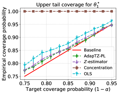
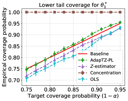
(a)		(b)

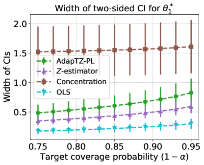
(c)

Figure 2: Average coverage and width of confidence intervals for $\theta^{*}_{1}$ over $T=1000$ repetitions of an adaptive linear model. The errorbars denote $\pm 1$ standard error. Parameters: $d_{T}=2,d_{N}=5,n=500,n_{1}=125$, $C=2$ and $t=0.2$. (a) and (b): Coverage of level $1-\alpha$ one-sided confidence intervals for $\theta^{*}_{1}$. (c): Width of level $1-\alpha$ two-sided confidence intervals for $\theta^{*}_{1}$.

We compare the AdapTZ-PL estimator to three other procedures: (i) ordinary least squares; (ii) a DML $Z$-estimator based on the unweighted score function

$$\phi_{i}(\theta,h):=({x}_{i}-p_{i})(y_{i}-\langle{x}_{i},\,\theta\rangle-h({z}_{i}));$$ (36)

and (iii) a confidence interval derived from a standard concentration inequality (cf. Theorem 8 in Abbasi-Yadkori et al. [1].)  Figure 2 shows the empirical coverage probability and width of confidence intervals obtained from each method. We observe that the AdapTZ-PL method provides appropriate coverage for all confidence levels. However, while the ordinary least squares estimator and the $Z$-estimator provide valid upper tail coverage and have shorter confidence intervals, they are both downward biased [45] and fail to achieve proper lower tail coverage.

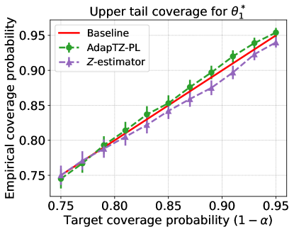
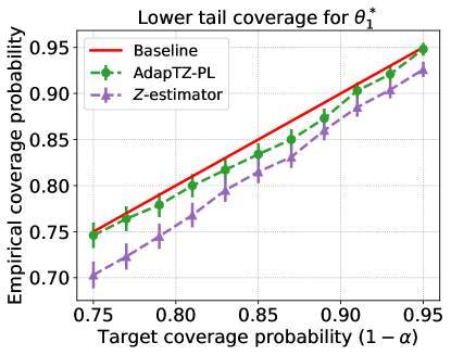
(a)		(b)

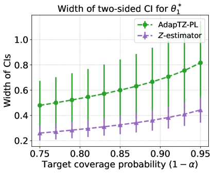
(c)

Figure 3: Average coverage and width of confidence intervals for $\theta^{*}_{1}$ over $1000$ repetitions of an adaptive linear model. The errorbars are $\pm 1$ standard error. Parameters: $d_{T}=2,d_{N}=1000,n=950,n_{1}=475$, $C=16$ and $t=0.2$. Left and Center: coverage of level $1-\alpha$ one-sided confidence intervals for $\theta^{*}_{1}$. Right: width of level $1-\alpha$ two-sided confidence intervals for $\theta^{*}_{1}$.

In the second experiment, we consider a linear model with high-dimensional nuisance. Namely, with the choice $(d_{T},d_{N})=(2,1000)$, we generate $n=950$ samples. Similar to the first experiment, we consider the no margin scenario where $\theta^{*}_{1}=\theta^{*}_{2}=2$. We also assume the linear model is sparse, in the sense that ${\eta}^{*}_{i}=0$ for $i>2$ and the first two coordinates of the nuisance parameter vector ${\eta}^{*}_{1},{\eta}^{*}_{2}$ are generated from $\mathcal{N}(0,\mathbf{I}_{2})$. We generate the samples in the same way as the first experiment, but use the LASSO estimator in both the data generating process and to obtain pilot estimates ${\widehat{\theta}},{\widehat{{\eta}}}$ of the parameters.

Figure 3 compares the coverage probability of AdapTZ and the standard DML $Z$-estimator. We see that the AdapTZ procedure achieves proper empirical coverage probability at most levels. Similar to the low dimensional case, while the $Z$-estimator has lower variance, it is downward biased and does not have proper coverage. We do not provide here the confidence interval derived from the concentration inequalities in Abbasi-Yadkori et al. [1] since the interval is too wide due to a $\sqrt{d/n}$ factor inside the bound.

4.2 Adaptive logistic model

We then demonstrate the usage of AdapTZ-GLM method when applied to a logistic regression model with adaptively collected data. We generate the data via the same procedure as in Section 4.2, but with several differences: (1). we assume ${z}_{i}$ are generated from an autoregressive process ${z}_{i}=\gamma{z}_{i-1}+W_{i}$, where ${z}_{0}:=0$ and $W_{i}$ are i.i.d. random variables following $\mathcal{N}(0,\mathbf{I}_{d_{N}})$. (2). We use the maximum likelihood estimator for logistic regression to estimate $\theta^{*},{\eta}^{*}$ in the data generating process and to obtain pilot estimators ${\widehat{\theta}},{\widehat{{\eta}}}$. (3). The responses $y_{i}$ are Bernoulli random variables with mean $g\big{(}\langle{x}_{i},\,\theta^{*}\rangle+\langle{z}_{i},\,{\eta}^{*}\rangle\big{)}$ given $\mathcal{F}_{i-1},{x}_{i},{z}_{i}$. In this example, we investigate the low-dimensional case where $d_{T}=2,d_{N}=20$ and the number of samples $n=2000$. Again, we choose $\theta^{*}_{1}=\theta^{*}_{2}=2$ and let ${\eta}^{*}$ be a fixed vector generated from $\mathcal{N}(0,\mathbf{I}_{d_{N}})$. Moreover, we use the MLE as the pilot estimator for $\theta^{*},{\eta}^{*}$ using $n_{1}=n/2=1000$ samples. From Figure 4, we observe that both AdapTZ and $Z$-estimator have upper tail coverage over the prespecified level. However, the $Z$-estimator as well as the MLE fail to achieve appropriate lower tail coverage. This is consistent with our previous observations in the linear model. Additionally, it should be noted that the empirical coverage probability of AdapTZ is not perfectly aligned with the baseline, likely due to the relatively small sample size.

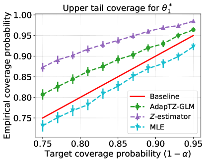
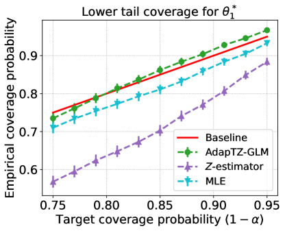
(a)		(b)

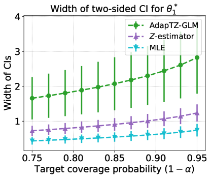
Figure 4: Average coverage and width of confidence intervals for $\theta^{*}_{1}$ over $1000$ repetitions of an adaptive logistic model. The error bars denote $\pm 1$ standard error. Parameters: $d_{T}=2,d_{N}=20,n=2000,n_{1}=1000$, $C=8$ and $t=0.1$. (a) and (b): coverage of level $1-\alpha$ one-sided confidence intervals for $\theta^{*}_{1}$. (c): Width of level $1-\alpha$ two-sided confidence intervals for $\theta^{*}_{1}$.

5 Proofs

We now turn to the proofs of our four general results, with Sections 5.1 through 5.4 devoted to the proofs of 1 through 4 respectively.

5.1 Proof of 1:

Recalling the definition (9) of the score function $\phi_{i}$, note that it is linear in the parameter vectors $\theta$ and $h$, and that we have the convenient decomposition

$$\widehat{\mathbb{E}}_{n_{2}}\phi_{i}(\theta,h)=(\widehat{\mathbb{E}}_{n_{2}}v_{i}{x}_{i}^{\top})(\theta-\theta^{*})+\widehat{\mathbb{E}}_{n_{2}}v_{i}\varepsilon_{i}-\widehat{\mathbb{E}}_{n_{2}}v_{i}(h({z}_{i})-h^{*}({z}_{i})),$$

where $v_{i}:={\mathbf{\Sigma}}_{i}^{-1/2}({x}_{i}-p_{i})$. By the definition of our $Z$-estimator, the pair $({\widetilde{\theta}},\widehat{h})$ satisfies the condition $\widehat{\mathbb{E}}_{n_{2}}\phi_{i}({\widetilde{\theta}},\widehat{h})=0$. Re-arranging this equality and multiplying both sides by $\sqrt{n_{2}}$ yields

$$\sqrt{n_{2}}(\widehat{\mathbb{E}}_{n_{2}}v_{i}{x}_{i}^{\top})({\widetilde{\theta}}-\theta^{*}) =\sqrt{n_{2}}\big{\{}\widehat{\mathbb{E}}_{n_{2}}v_{i}\varepsilon_{i}-\widehat{\mathbb{E}}_{n_{2}}v_{i}(\widehat{h}({z}_{i})-h^{*}({z}_{i}))\big{\}}.$$ (37)

We next analyze equation (37) via the following three results which we prove in 2, 3 and 4 (see details in Section C.1) respectively.

$$\widehat{\mathbb{E}}_{n_{2}}\sqrt{n_{2}}v_{i}\varepsilon_{i}\stackrel{{\scriptstyle d}}{{\rightarrow}}\mathcal{N}(0,\sigma^{2}\mathbf{I}_{d_{T}})$$ (38a)

$$\widehat{\mathbb{E}}_{n_{2}}\sqrt{n_{2}}v_{i}(\widehat{h}({z}_{i})-h^{*}({z}_{i}))\overset{p}{\to}0$$ (38b)

$$|\mkern-2.0mu|\mkern-2.0mu|\widehat{\mathbb{E}}_{n_{2}}v_{i}{x}_{i}^{\top}-\widehat{\mathbb{E}}_{n_{2}}{\mathbf{\Sigma}}_{i}^{1/2}|\mkern-2.0mu|\mkern-2.0mu|_{{\mathrm{op}}}=o_{p}(\sigma_{\min}(\widehat{\mathbb{E}}_{n_{2}}{\mathbf{\Sigma}}_{i}^{1/2}))$$ (38c)

With these three results at hand, the rest of the proof is straightforward. Indeed, substituting the conditions (38a) and  (38b) into equation (37) and applying Slutsky’s theorem yields

$$(\widehat{\mathbb{E}}_{n_{2}}v_{i}{x}_{i}^{\top})\sqrt{n_{2}}({\widetilde{\theta}}-\theta^{*})\stackrel{{\scriptstyle d}}{{\rightarrow}}\mathcal{N}(0,\sigma^{2}\mathbf{I}_{d_{T}}),$$ (39)

and the distributional convergence statement also implies $\|(\widehat{\mathbb{E}}_{n_{2}}v_{i}{x}_{i}^{\top})\sqrt{n_{2}}({\widetilde{\theta}}-\theta^{*})\|_{2}=\mathcal{O}_{p}(1)$ by continuous mapping theorem, definition of weak convergence and boundedness in probability. Combining the last implication with the bound (38c) yields

$$\|(\widehat{\mathbb{E}}_{n_{2}}{\mathbf{\Sigma}}_{i}^{1/2}\sqrt{n_{2}}({\widetilde{\theta}}-\theta^{*})\|_{2} \leq\|(\widehat{\mathbb{E}}_{n_{2}}v_{i}{x}_{i}^{\top})\sqrt{n_{2}}({\widetilde{\theta}}-\theta^{*})\|_{2}+\|(\widehat{\mathbb{E}}_{n_{2}}(v_{i}{x}_{i}^{\top}-{\mathbf{\Sigma}}_{i}^{1/2})\sqrt{n_{2}}({\widetilde{\theta}}-\theta^{*})\|_{2}$$

$$=\mathcal{O}_{p}(1)+o_{p}(\|(\widehat{\mathbb{E}}_{n_{2}}{\mathbf{\Sigma}}_{i}^{1/2}\sqrt{n_{2}}({\widetilde{\theta}}-\theta^{*})\|_{2}).$$

Putting together the pieces we have ${\|(\widehat{\mathbb{E}}_{n_{2}}{\mathbf{\Sigma}}_{i}^{1/2}\sqrt{n_{2}}({\widetilde{\theta}}-\theta^{*})\|_{2}=\mathcal{O}_{p}(1)}$, and consequently we deduce

$$\|(\widehat{\mathbb{E}}_{n_{2}}(v_{i}{x}_{i}^{\top}-{\mathbf{\Sigma}}_{i}^{1/2})\sqrt{n_{2}}({\widetilde{\theta}}-\theta^{*})\|_{2}=o_{p}(1)$$

Finally, combining the last result with the convergence statement (39) and applying the Slusky’s theorem we conclude

$$(\widehat{\mathbb{E}}_{n_{2}}{\mathbf{\Sigma}}_{i}^{1/2})\sqrt{n_{2}}({\widetilde{\theta}}-\theta^{*})\stackrel{{\scriptstyle d}}{{\rightarrow}}\mathcal{N}(0,\sigma^{2}\mathbf{I}_{d_{T}}).$$

This completes the proof of 1.

5.2 Proof of 2

The proof of this theorem is essentially the same as that of 1 but with a different weighting vector. Let us introduce the shorthand

$$w_{i1} :=\langle A_{i1},\,{x}_{i}-p_{i}({z}_{i},\mathcal{F}_{i-1})\rangle\in\real.$$

Following a decomposition similar to equation (37), we have

$$(\widehat{\mathbb{E}}_{n_{2}}w_{i1}\langle{x}_{i},\,u\rangle)\sqrt{n_{2}}({\widetilde{\theta}}_{u}-\theta^{*}_{u})+[\widehat{\mathbb{E}}_{n_{2}}w_{i1}{x}_{i}^{\top}(\mathbf{I}_{d_{T}}-uu^{\top})]\sqrt{n_{2}}({\widehat{\theta}}-\theta^{*})$$

$$=[\widehat{\mathbb{E}}_{n_{2}}\sqrt{n_{2}}w_{i1}\varepsilon_{i}-\widehat{\mathbb{E}}_{n_{2}}\sqrt{n_{2}}w_{i1}(\widehat{h}({z}_{i})-h^{*}({z}_{i}))].$$ (40)

We prove the following three results in 5, 6 and 7 respectively (see details in Section C.2), which analyze the three terms in the last decomposition.

$$\widehat{\mathbb{E}}_{n_{2}}\sqrt{n_{2}}w_{i1}\varepsilon_{i}\stackrel{{\scriptstyle d}}{{\rightarrow}}\mathcal{N}(0,\sigma^{2})$$ (41a)

$$\widehat{\mathbb{E}}_{n_{2}}\sqrt{n_{2}}w_{i1}({\widehat{{\eta}}}({z}_{i})-{\eta}^{*}({z}_{i}))\overset{p}{\to}0$$ (41b)

$$\Big{|}\widehat{\mathbb{E}}_{n_{2}}w_{i1}{x}_{i}^{\top}u-\widehat{\mathbb{E}}_{n_{2}}\frac{1}{\sqrt{u^{\top}{\mathbf{\Sigma}}_{i}^{-1}u}}\Big{|}=o_{p}\Big{(}\Big{|}\widehat{\mathbb{E}}_{n_{2}}\frac{1}{\sqrt{u^{\top}{\mathbf{\Sigma}}_{i}^{-1}u}}\Big{|}\Big{)}.$$ (41c)

Assuming these three results are given at the moment, plugging equation (41a), (41b) into (5.2) we deduce

$$(\widehat{\mathbb{E}}_{n_{2}}w_{i1}{x}_{i}^{\top}u)\sqrt{n_{2}}({\widetilde{\theta}}_{u}-\theta^{*}_{u})+[\widehat{\mathbb{E}}_{n_{2}}w_{i1}{x}_{i}^{\top}(\mathbf{I}_{d_{T}}-uu^{\top})]\sqrt{n_{2}}({\widehat{\theta}}-\theta^{*})\stackrel{{\scriptstyle d}}{{\rightarrow}}\mathcal{N}(0,\sigma^{2}).$$ (42)

Moreover, invoking the bound (41c) we have

$$\Big{(}\widehat{\mathbb{E}}_{n_{2}}w_{i1}{x}_{i}^{\top}u-\widehat{\mathbb{E}}_{n_{2}}\frac{1}{\sqrt{u^{\top}{\mathbf{\Sigma}}_{i}^{-1}u}}\Big{)}\sqrt{n_{2}}({\widetilde{\theta}}_{1}-\theta^{*}_{1}) =o_{p}\Big{(}\widehat{\mathbb{E}}_{n_{2}}\frac{1}{\sqrt{u^{\top}{\mathbf{\Sigma}}_{i}^{-1}u}}\sqrt{n_{2}}({\widetilde{\theta}}_{1}-\theta^{*}_{1})\Big{)}$$ (43)

Putting equation (42), (43) together, it remains to show

$$\widehat{\mathbb{E}}_{n_{2}}w_{i1}{x}_{i}^{\top}(\mathbf{I}_{d_{T}}-uu^{\top})\sqrt{n_{2}}({\widehat{\theta}}-\theta^{*})=o_{p}(1).$$ (44)

Proof of equation (44):

Observe that $\mathbb{E}(w_{i1}{x}_{i}^{\top}\mid\mathcal{F}_{i-1})=0$, which implies that $\{w_{i1}{x}_{i}^{\top}\}_{i\geq 1}$ forms a martingale difference sequence. We have

$$\mathbb{E}\|\sqrt{n_{2}}\widehat{\mathbb{E}}_{n_{2}}w_{i1}{x}_{i}^{\top}\|_{2}^{2} =\frac{1}{n_{2}}\sum_{i=n_{1}+1}^{n}\mathbb{E}\|w_{i1}{x}_{i}^{\top}\|_{2}^{2}$$

$$\leq\frac{1}{n_{2}}\sum_{i=n_{1}+1}^{n}\mathbb{E}w_{i1}^{2}=1,$$

where the last line follows from the bound $\|{x}_{i}^{\top}\|_{2}\leq 1$ and noting that $\mathbb{E}w_{i1}^{2}=1$. Thus, we conclude that ${\sqrt{n_{2}}\widehat{\mathbb{E}}_{n_{2}}w_{i1}{x}_{i}^{\top}=\mathcal{O}_{p}(1)}$. Combining this fact with the assumption that $(\mathbf{I}_{d_{T}}-uu^{\top})({\widehat{\theta}}-\theta^{*})\overset{p}{\to}0$ yields the claim.

5.3 Proof of 3

For notational simplicity, we only prove the result when the nuisance function is linear, i.e., $h^{*}({z})=\langle{z},\,{\eta}^{*}\rangle$ for some ${\eta}^{*}\in\mathcal{H}\in\mathbb{R}^{d_{N}}$. The proof general nuisance function $h$ is essentially the same with $\langle{z},\,{\eta}\rangle$ replaced by $h({z})$. See Section 5.3.3 for more details.

For the linear nuisance function $h^{*}({z})=\langle{z},\,{\eta}^{*}\rangle$, the GLM assumptions and Assumption (NUI^′)10pt can be replaced by the following two simplified versions:

• (Bounded covariates and nuisance) There exist $M_{{\eta}},M_{\omega}>0$ such that $\sup_{{\eta}\in\mathcal{H}}\|{\eta}\|_{2}\leq M_{{\eta}}$ and $\|({x}_{i}^{\top},{z}_{i}^{\top})\|_{2}\leq D_{x}$;

• (Accuracy of pilot estimates) The pilot estimator ${\widehat{{\eta}}}\in\mathcal{H}$ from Step 3 of AdapTZ-GLM satisfies $\|{\widehat{{\eta}}}-{\eta}^{*}\|_{2}=o_{p}(n^{-1/4})$.

5.3.1 Main argument

Substituting the definition of $\phi_{i}$ from equation (18) into the estimating equation (21), we find that

$$\sqrt{n_{2}}\widehat{\mathbb{E}}_{n_{2}}\widehat{}\mathbf{\Omega}_{i}({x}_{i}-\widehat{m}_{i})\varepsilon_{i}$$ (45a)

. $$=\sqrt{n_{2}}\widehat{\mathbb{E}}_{n_{2}}\widehat{}\mathbf{\Omega}_{i}({x}_{i}-\widehat{m}_{i})(g({x}_{i}^{\top}{\widetilde{\theta}}+{z}_{i}^{\top}{\widehat{{\eta}}})-g({x}_{i}^{\top}\theta^{*}+{z}_{i}^{\top}{\eta}^{*})).$$ (45b)

Focusing on the preceding equation, we now perform a second order Taylor series expansion of $g$ around the point $({\widehat{\theta}},{\widehat{{\eta}}})$, thereby obtaining we obtain

$$\sqrt{n_{2}}\widehat{\mathbb{E}}_{n_{2}}\widehat{}\mathbf{\Omega}_{i}({x}_{i}-\widehat{m}_{i})\varepsilon_{i}$$

$$=\sqrt{n_{2}}\widehat{\mathbb{E}}_{n_{2}}\widehat{}\mathbf{\Omega}_{i}({x}_{i}-\widehat{m}_{i})g^{\prime}\big{(}\langle{x}_{i},\,{\widehat{\theta}}\rangle+\langle{z}_{i},\,{\widehat{{\eta}}}\rangle\big{)}({x}_{i}-\widehat{m}_{i})^{\top}({\widetilde{\theta}}-\theta^{*})$$

$$\quad+\sqrt{n_{2}}\widehat{\mathbb{E}}_{n_{2}}\widehat{}\mathbf{\Omega}_{i}({x}_{i}-\widehat{m}_{i})\Big{[}Q_{1}+Q_{2}+Q_{3}+Q_{4}\Big{]},$$ (46)

where

$$Q_{1} :=g^{\prime}(\langle{x}_{i},\,{\widehat{\theta}}\rangle+\langle{z}_{i},\,{\widehat{{\eta}}}\rangle)\langle{z}_{i},\,{\widehat{{\eta}}}-{\eta}^{*}\rangle$$

$$Q_{2} :=g^{\prime}\big{(}\langle{x}_{i},\,{\widehat{\theta}}\rangle+\langle{z}_{i},\,{\widehat{{\eta}}}\rangle\big{)}\widehat{m}_{i}^{\top}({\widetilde{\theta}}-\theta^{*})$$

$$Q_{3} :=\frac{1}{2}\int^{1}_{0}\int^{1}_{0}g^{\prime\prime}\big{(}\langle{x}_{i},\,{\widehat{\theta}}+r_{1}r_{2}({\widetilde{\theta}}-{\widehat{\theta}})\rangle+\langle{z}_{i},\,{\widehat{{\eta}}}\rangle\big{)}|\langle{x}_{i},\,{\widetilde{\theta}}-{\widehat{\theta}}\rangle|^{2}dr_{1}dr_{2},\quad\mbox{and}$$

$$Q_{4} :=-\frac{1}{2}\int^{1}_{0}\int^{1}_{0}g^{\prime\prime}\big{(}\langle{x}_{i},\,{\widehat{\theta}}+r_{1}r_{2}(\theta^{*}-{\widehat{\theta}})\rangle+\langle{z}_{i},\,{\widehat{{\eta}}}+r_{1}r_{2}({\eta}^{*}-{\widehat{{\eta}}})\rangle\big{)}|\langle{x}_{i},\,\theta^{*}-{\widehat{\theta}}\rangle+\langle{z}_{i},\,{\eta}^{*}-{\widehat{{\eta}}}\rangle|^{2}dr_{1}dr_{2}.$$

We complete the proof by establishing the following three results.

$$\sqrt{n_{2}}\widehat{\mathbb{E}}_{n_{2}}\widehat{}\mathbf{\Omega}_{i}({x}_{i}-\widehat{m}_{i})\varepsilon_{i}\stackrel{{\scriptstyle d}}{{\rightarrow}}\mathcal{N}(0,\mathbf{I}_{d_{T}})$$ (48a)

If $${\widetilde{\theta}}-\theta^{*}=o_{p}(1)$$, then we have

$$\sqrt{n_{2}}\widehat{\mathbb{E}}_{n_{2}}\widehat{}\mathbf{\Omega}_{i}({x}_{i}-\widehat{m}_{i})(Q_{1}+Q_{2})\overset{p}{\to}0$$ (48b)

If $${\widetilde{\theta}}-\theta^{*}=o_{p}(n^{-t})$$, then

$$\quad\sqrt{n_{2}}\widehat{\mathbb{E}}_{n_{2}}\widehat{}\mathbf{\Omega}_{i}({x}_{i}-\widehat{m}_{i})(Q_{3}+Q_{4})$$

$$=o_{p}(1)+o_{p}(\|\sqrt{n_{2}}\widehat{\mathbb{E}}_{n_{2}}\widehat{}\mathbf{\Omega}_{i}({x}_{i}-\widehat{m}_{i})g^{\prime}\big{(}\langle{x}_{i},\,{\widehat{\theta}}\rangle+\langle{z}_{i},\,{\widehat{{\eta}}}\rangle\big{)}({x}_{i}-\widehat{m}_{i})^{\top}({\widetilde{\theta}}-\theta^{*})\|_{2}).$$ (48c)

We prove the claims (48a), (48b) and (48c) in Lemmas 9, 10 and 11, respectively (see details in Section C.3). We also verify in a moment that

$${\widetilde{\theta}}-\theta^{*}=o_{p}(n^{-t}).$$ (49)

With the last four results at hand, the proof of 3 is immediate. Indeed, denoting $\sqrt{n_{2}}\widehat{\mathbb{E}}_{n_{2}}\widehat{}\mathbf{\Omega}_{i}({x}_{i}-\widehat{m}_{i})g^{\prime}\big{(}\langle{x}_{i},\,{\widehat{\theta}}\rangle+\langle{z}_{i},\,{\widehat{{\eta}}}\rangle\big{)}({x}_{i}-\widehat{m}_{i})^{\top}({\widetilde{\theta}}-\theta^{*})$ by $Q_{0}$ and substituting results above into (46) and using Slusky’s theorem yields

$$Q_{0}+o_{p}(|\mkern-2.0mu|\mkern-2.0mu|Q_{0}|\mkern-2.0mu|\mkern-2.0mu|_{{\mathrm{op}}})\stackrel{{\scriptstyle d}}{{\rightarrow}}\mathcal{N}(0,\mathbf{I}_{d_{T}}).$$ (50)

Since $\mathcal{N}(0,\mathbf{I}_{d_{T}})=\mathcal{O}_{p}(1)$, we have $Q_{0}=\mathcal{O}_{p}(1)$ and hence $o_{p}(|\mkern-2.0mu|\mkern-2.0mu|Q_{0}|\mkern-2.0mu|\mkern-2.0mu|_{{\mathrm{op}}})=o_{p}(1)$. This together with Slusky’s theorem yields the result as desired. It remains to prove the consistency condition (49).

5.3.2 Proof of consistency condition (49)

We use an inductive argument on $k$. More precisely, we first establish $o_{p}(n^{-(\delta\wedge t)})$-consistency for the base case $k=1$. In the inductive step, we assume that $o_{p}(n^{-(k\delta\wedge t)})$-consistency holds for some $k\geq 1$, and then prove that it holds at step $(k+1)$—that is, $o_{p}(n^{-((k+1)\delta\wedge t)})$-consistency holds.

Base case:

We start by proving $o_{p}(n^{-(\delta\wedge t)})$-consistency.

Introduce the shorthand $\omega:=({\makebox[0.0pt][l]{\hskip 2.08334pt\rule[8.23611pt]{2.48053pt}{0.43057pt}}{\theta}},{\eta})$, $\widehat{\omega}:=({\widehat{\theta}},{\widehat{{\eta}}})$ for the estimator computed in Step 3 of AdapTZ-GLM, and $\omega^{*}:=(\theta^{*},{\eta}^{*})$.

By the triangle inequality, we have

$$\|\widetilde{\mathbb{E}}_{n_{2}}\phi_{i}({\widetilde{\theta}},\omega^{*})\|_{2} \leq\|(\widetilde{\mathbb{E}}_{n_{2}}\phi_{i}({\widetilde{\theta}},\omega^{*})-\widetilde{\mathbb{E}}_{n_{2}}\phi_{i}({\widetilde{\theta}},\widehat{\omega})\|_{2}+\|(\widetilde{\mathbb{E}}_{n_{2}}-\widehat{\mathbb{E}}_{n_{2}})\phi_{i}({\widetilde{\theta}},\widehat{\omega})\|_{2}$$

$$\quad+\|(\widehat{\mathbb{E}}_{n_{2}}\phi_{i}({\widetilde{\theta}},\widehat{\omega})\|_{2}$$

$$\leq\|(\widetilde{\mathbb{E}}_{n_{2}}\phi_{i}({\widetilde{\theta}},\omega^{*})-\widetilde{\mathbb{E}}_{n_{2}}\phi_{i}({\widetilde{\theta}},\widehat{\omega})\|_{2}+\|(\widehat{\mathbb{E}}_{n_{2}}-\widetilde{\mathbb{E}}_{n_{2}})\phi_{i}({\widetilde{\theta}},\widehat{\omega})\|_{2}$$

$$\quad+\|\widehat{\mathbb{E}}_{n_{2}}\phi_{i}(\theta^{*},\widehat{\omega})\|_{2}$$

$$\leq 2\sup_{\theta\in\Theta}\|\widetilde{\mathbb{E}}_{n_{2}}\phi_{i}(\theta,\omega^{*})-\widetilde{\mathbb{E}}_{n_{2}}\phi_{i}(\theta,\widehat{\omega})\|_{2}$$

$$\quad+2\sup_{\theta\in\Theta}\|(\widehat{\mathbb{E}}_{n_{2}}-\widetilde{\mathbb{E}}_{n_{2}})\phi_{i}(\theta,\widehat{\omega})\|_{2},$$

$$=:2\Re_{1}+2\Re_{2},$$ (51)

where the second uses the definition of ${\widetilde{\theta}}$ that $\widehat{\mathbb{E}}_{n_{2}}\phi_{i}({\widetilde{\theta}},\widehat{\omega})=0$, and the third inequality follows from the triangle inequality and the fact that $\widetilde{\mathbb{E}}_{n_{2}}\phi_{i}(\theta^{*},\theta^{*},{\eta}^{*})=0$.

Since $\quad\|\widetilde{\mathbb{E}}_{n_{2}}\phi_{i}(\theta,\omega^{*})-\widetilde{\mathbb{E}}_{n_{2}}\phi_{i}(\theta,\widehat{\omega})\|_{2}\leq L_{\phi,1}\|\widehat{\omega}-\omega^{*}\|_{2}$ for some constant $L_{\phi,1}>0$ by 14, it follows that $\Re_{1}=o_{p}(n^{-1/4}).$ For $\Re_{2}$, it follows from 13 that $\Re_{2}=\mathcal{O}_{p}(\log n/\sqrt{n})$.

Combining the results above, we obtain $\|\widetilde{\mathbb{E}}_{n_{2}}\phi_{i}({\widetilde{\theta}},\omega^{*})\|_{2}=o_{p}(n^{-1/4})$. On the other hand,

$$\|\widetilde{\mathbb{E}}_{n_{2}}\phi_{i}({\widetilde{\theta}},\omega^{*})\|_{2}$$

$$=\|\widetilde{\mathbb{E}}_{n_{2}}(\phi_{i}({\widetilde{\theta}},\omega^{*})-\phi_{i}(\theta^{*},\omega^{*}))\|_{2}$$

$$\geq\frac{1}{2}\|\widetilde{\mathbb{E}}_{n_{2}}\partial_{\theta}\phi_{i}(\theta^{*},\omega^{*})({\widetilde{\theta}}-\theta^{*})\|_{2}\wedge c_{\phi}n^{-1/4}$$

$$\geq\frac{1}{2}\sigma_{\min}(\widetilde{\mathbb{E}}_{n_{2}}\partial_{\theta}\phi_{i}(\theta^{*},\omega^{*}))\|{\widetilde{\theta}}-\theta^{*}\|_{2}\wedge c_{\phi}n^{-1/4}$$

$$\geq\frac{m_{\phi}}{2}n^{\delta-t}\|{\widetilde{\theta}}-\theta^{*}\|_{2}\wedge c_{\phi}n^{-1/4}$$

with probability converging to one. Here the inequalities follows from the identifiability assumption in 3. Therefore,

$$o_{p}(n^{-1/4})=\|\widetilde{\mathbb{E}}_{n_{2}}\phi({\widetilde{\theta}},\omega^{*})\|_{2}\geq m_{\phi}n^{\delta-t}\|{\widetilde{\theta}}-\theta^{*}\|_{2}/2\wedge c_{\phi}n^{-1/4}$$ (52)

with probability converging to one. Since $t\leq 1/4$, it follows directly that $\|{\widetilde{\theta}}-\theta^{*}\|_{2}=o_{p}(n^{-\delta})=o_{p}(n^{-(\delta\wedge t)})$.

Inductive step:

Next we show that given ${\widetilde{\theta}}-\theta^{*}=o_{p}(n^{-(k\delta\wedge t)})$, we have ${\widetilde{\theta}}-\theta^{*}=o_{p}(n^{-((k+1)\delta\wedge t)})$. In fact, it suffices to show that $\|\widetilde{\mathbb{E}}_{n_{2}}\phi_{i}({\widetilde{\theta}},\omega^{*})\|_{2}=o_{p}(n^{-1/4-(k\delta\wedge t)})$ for any $t\in(k\delta,1/4]$. This is because combining it with the high probability lower bound $m_{\phi}n^{-t}\|{\widetilde{\theta}}-\theta^{*}\|_{2}$ from equation (52) directly gives $\|{\widetilde{\theta}}-\theta^{*}\|_{2}=o_{p}(n^{-((k+1)\delta\wedge t)})$ as desired.

Following the same steps as in the upper bound (51) and using the result that $\Re_{2}=\mathcal{O}_{p}(\log n/\sqrt{n})$, we obtain

$$\|\widetilde{\mathbb{E}}_{n_{2}}\phi_{i}({\widetilde{\theta}},\omega^{*})\|_{2} \leq\|(\widetilde{\mathbb{E}}_{n_{2}}\phi_{i}({\widetilde{\theta}},\omega^{*})-\widetilde{\mathbb{E}}_{n_{2}}\phi_{i}({\widetilde{\theta}},\widehat{\omega})\|+\|(\widetilde{\mathbb{E}}_{n_{2}}-\widehat{\mathbb{E}}_{n_{2}})\phi_{i}({\widetilde{\theta}},\widehat{\omega})\|_{2}$$

$$\quad+\|(\widehat{\mathbb{E}}_{n_{2}}\phi_{i}({\widetilde{\theta}},\widehat{\omega})\|_{2}$$

$$\leq\|(\widetilde{\mathbb{E}}_{n_{2}}\phi_{i}({\widetilde{\theta}},\omega^{*})-\widetilde{\mathbb{E}}_{n_{2}}\phi_{i}({\widetilde{\theta}},\widehat{\omega})\|_{2}+\|(\widehat{\mathbb{E}}_{n_{2}}-\widetilde{\mathbb{E}}_{n_{2}})\phi_{i}({\widetilde{\theta}},\widehat{\omega})\|_{2}$$

$$\quad+\|\widehat{\mathbb{E}}_{n_{2}}\phi_{i}(\theta^{*},\widehat{\omega})\|_{2}$$

$$\leq 2\sup_{\theta\in\Theta,\|\theta-\theta^{*}\|\leq n^{-(k\delta\wedge t)}}\|\widetilde{\mathbb{E}}_{n_{2}}\phi_{i}(\theta,\omega^{*})-\widetilde{\mathbb{E}}_{n_{2}}\phi_{i}(\theta,\widehat{\omega})\|$$

$$\quad+2\sup_{\theta\in\Theta}\|(\widehat{\mathbb{E}}_{n_{2}}-\widetilde{\mathbb{E}}_{n_{2}})\phi_{i}(\theta,\widehat{\omega})\|_{2},$$

$$=2\sup_{\theta\in\Theta,\|\theta-\theta^{*}\|_{2}\leq n^{-(k\delta\wedge t)}}\|\widetilde{\mathbb{E}}_{n_{2}}\phi_{i}(\theta,\omega^{*})-\widetilde{\mathbb{E}}_{n_{2}}\phi_{i}(\theta,\widehat{\omega})\|_{2}+\mathcal{O}_{p}(\log n/\sqrt{n}).$$ (53)

Denote $\{\theta\in\Theta,\|\theta-\theta^{*}\|_{2}\leq n^{-(k\delta\wedge t)}\}$ by $\mathcal{C}_{k}$. Then

$$\sup_{\mathcal{C}_{k}}\|\widetilde{\mathbb{E}}_{n_{2}}\phi_{i}(\theta,\omega^{*})-\widetilde{\mathbb{E}}_{n_{2}}\phi_{i}(\theta,\widehat{\omega})\|_{2}$$

$$\leq\sup_{\mathcal{C}_{k}}\|\widetilde{\mathbb{E}}_{n_{2}}\partial_{\omega}\phi_{i}(\theta,\omega^{*})(\widehat{\omega}-\omega^{*})$$

$$+\frac{1}{2}(\widehat{\omega}-\omega^{*})^{\top}\Big{[}\int_{0}^{1}\int_{0}^{1}\widetilde{\mathbb{E}}_{n_{2}}\partial^{2}_{\omega}\phi_{i}(\theta,\omega^{*}+r_{1}r_{2}(\widehat{\omega}-\omega^{*}))dr_{1}dr_{2}\Big{]}(\widehat{\omega}-\omega^{*})\|_{2}$$

$$\lesssim\sup_{\mathcal{C}_{k}}\|[\widetilde{\mathbb{E}}_{n_{2}}\partial_{\omega}\phi_{i}(\theta,\omega^{*})-\widetilde{\mathbb{E}}_{n_{2}}\partial_{\omega}\phi_{i}(\theta^{*},\omega^{*})](\widehat{\omega}-\omega^{*})\|_{2}+L_{\phi,2}\|\widehat{\omega}-\omega^{*}\|_{2}^{2}$$

$$\leq\sup_{\mathcal{C}_{k}}L_{\phi,1}\|{\widetilde{\theta}}-\theta^{*}\|_{2}\|\widehat{\omega}-\omega^{*}\|_{2}+L_{\phi,2}\|\widehat{\omega}-\omega^{*}\|_{2}^{2}=o_{p}(n^{-(k\delta\wedge t)-1/4}),$$ (54)

where $L_{\phi,1},L_{\phi,2}>0$ are some constants introduced in 14. In the second line we use Taylor expansion, the second inequality follows from Neyman orthogonality $\widetilde{\mathbb{E}}_{n_{2}}\partial_{\omega}\phi_{i}(\theta^{*},\omega^{*})=0$ and 14, and the last line is also due to 14 and the assumption that $\widehat{\omega}-\omega^{*}=o_{p}(n^{-1/4})$ and ${\widetilde{\theta}}-\theta^{*}=o_{p}(n^{-(k\delta\wedge t)})$. Since $(k\delta\wedge t)+1/4<1/2$, we conclude by combining (53) and (54) that $\|\widetilde{\mathbb{E}}_{n_{2}}\phi_{i}({\widetilde{\theta}},\omega^{*})\|_{2}=o_{p}(n^{-(k\delta\wedge t)-1/4})$.

5.3.3 Proof for general nuisance function $h$:

We remark that the proof for general nuisance function $h$ is essentially the same with, ${z}^{\top}{\eta}$ replaced by $h({z})$. This is because in the proof we only invoke our assumption on the estimation error $\|\widehat{h}({z})-h^{*}({z})\|_{\infty}$ and does not exploit the specific form of $h$. However, by assuming a linear parameterization on $h$, we can avoid the usage of Gateaux derivative and hence simplify our notation of the gradient of the score function.

5.4 Proof of 4

The proof of this theorem is similar to the proof of 3, and we only prove it for linear nuisance, i.e., $h^{*}({z})=\langle{z},\,{\eta}^{*}\rangle$. We only provide a proof sketch for brevity.

Substituting the definition of $\phi_{i1}$ into the estimating equation (25) yields

$$\sqrt{n_{2}}\widehat{\mathbb{E}}_{n_{2}}\widehat{A}_{i1}({z}_{i},\mathcal{F}_{i-1})({x}_{i}-\widehat{m}_{i}({z}_{i},\mathcal{F}_{i-1}))\varepsilon_{i}$$

$$=\sqrt{n_{2}}\widehat{\mathbb{E}}_{n_{2}}\widehat{A}_{i1}({x}_{i}-\widehat{m}_{i})\cdot$$

$$\quad\Big{[}g\big{(}\langle{x}_{i},\,u\rangle{\widetilde{\theta}}_{u}+{x}_{i}^{\top}(\mathbf{I}_{d_{T}}-uu^{\top}){\widehat{\theta}}+\langle{z}_{i},\,{\widehat{{\eta}}}\rangle\big{)}-g\big{(}\langle{x}_{i},\,u\rangle\theta^{*}_{u}+{x}_{i}^{\top}(\mathbf{I}_{d_{T}}-uu^{\top})\theta^{*}+\langle{z}_{i},\,{\eta}^{*}\rangle\big{)}\Big{]}.$$

Throughout, we use the shorthand ${\widehat{\theta}}_{u}:=\langle u,\,{\widehat{\theta}}\rangle$. Performing a second order Taylor series expansion of $g$ on the right-hand side of the last equation at $({\widehat{\theta}}_{u},{\widehat{\theta}},{\widehat{{\eta}}})$, we obtain

$$\quad\sqrt{n_{2}}\widehat{\mathbb{E}}_{n_{2}}\widehat{A}_{i1}({z}_{i},\mathcal{F}_{i-1})({x}_{i}-\widehat{m}_{i}({z}_{i},\mathcal{F}_{i-1}))\varepsilon_{i}$$ (55)

$$=\sqrt{n_{2}}\widehat{\mathbb{E}}_{n_{2}}\widehat{A}_{i1}({x}_{i}-\widehat{m}_{i})g^{\prime}\big{(}\langle{x}_{i},\,{\widehat{\theta}}\rangle+\langle{z}_{i},\,{\widehat{{\eta}}}\rangle\big{)}({x}_{i}-\widehat{m}_{i})^{\top}u({\widetilde{\theta}}_{u}-\theta^{*}_{u})$$

$$\quad+\sqrt{n_{2}}\widehat{\mathbb{E}}_{n_{2}}\widehat{A}_{i1}({x}_{i}-\widehat{m}_{i})\Big{[}\widetilde{Q}_{1}+\widetilde{Q}_{2}+\widetilde{Q}_{3}+\widetilde{Q}_{4}\Big{]},$$ (56)

where

$$\widetilde{Q}_{1} =g^{\prime}\big{(}\langle{x}_{i},\,{\widehat{\theta}}\rangle+\langle{z}_{i},\,{\widehat{{\eta}}}\rangle\big{)}[{x}_{i}^{\top}(\mathbf{I}_{d_{T}}-uu^{\top})({\widehat{\theta}}-\theta^{*})+\langle{z}_{i},\,{\widehat{{\eta}}}-{\eta}^{*}\rangle],$$

$$\widetilde{Q}_{2} =g^{\prime}\big{(}\langle{x}_{i},\,{\widehat{\theta}}\rangle+\langle{z}_{i},\,{\widehat{{\eta}}}\rangle\big{)}\langle\widehat{m}_{i},\,u\rangle({\widetilde{\theta}}_{u}-\theta^{*}_{u})$$

$$\widetilde{Q}_{3} =\frac{1}{2}\int^{1}_{0}\int^{1}_{0}g^{\prime\prime}\big{(}\langle{x}_{i},\,u\rangle({\widehat{\theta}}_{u}+r_{1}r_{2}({\widetilde{\theta}}_{u}-{\widehat{\theta}}_{u}))+{x}_{i}^{\top}(\mathbf{I}_{d_{T}}-uu^{\top}){\widehat{\theta}}+\langle{z}_{i},\,{\widehat{{\eta}}}\rangle\big{)}\big{|}\langle{x}_{i},\,u\rangle({\widetilde{\theta}}_{u}-{\widehat{\theta}}_{u})\big{|}^{2}dr_{1}dr_{2}$$

$$\widetilde{Q}_{4} =-\frac{1}{2}\int^{1}_{0}\int^{1}_{0}g^{\prime\prime}\big{(}\langle{x}_{i},\,u\rangle({\widehat{\theta}}_{u}+r_{1}r_{2}(\theta^{*}_{u}-{\widehat{\theta}}_{u}))+{x}_{i}^{\top}(\mathbf{I}_{d_{T}}-uu^{\top})({\widehat{\theta}}+r_{1}r_{2}(\theta^{*}-{\widehat{\theta}}))+\langle{z}_{i},\,{\widehat{{\eta}}}+r_{1}r_{2}({\eta}^{*}-{\widehat{{\eta}}})\rangle\big{)}.$$

Following an argument similar to 9, 10 and 11, it can be shown that

$$\sqrt{n_{2}}\widehat{\mathbb{E}}_{n_{2}}\widehat{A}_{i1}({z}_{i},\mathcal{F}_{i-1})({x}_{i}-\widehat{m}_{i}({z}_{i},\mathcal{F}_{i-1}))\varepsilon_{i} \stackrel{{\scriptstyle d}}{{\rightarrow}}\mathcal{N}(0,1),$$ (57a)

$$\sqrt{n_{2}}\widehat{\mathbb{E}}_{n_{2}}\widehat{A}_{i1}({x}_{i}-\widehat{m}_{i})(\widetilde{Q}_{1}+\widetilde{Q}_{2}) \overset{p}{\to}0$$ (57b)

$$\sqrt{n_{2}}\widehat{\mathbb{E}}_{n_{2}}\widehat{A}_{i1}({x}_{i}-\widehat{m}_{i})(\widetilde{Q}_{3}+\widetilde{Q}_{4}) \overset{p}{\to}0$$ (57c)

Here the claim (57c) requires the assumption ${\widetilde{\theta}}_{u}-\theta^{*}_{u}=o_{p}(n^{-t})$. We can prove this $o_{p}(n^{-t})$-consistency following arguments that are similar to those used in the proof of 3. Concretely, the proof is essentially the same except for replacing $\phi_{i}$ with $\phi_{i1}$ and showing $\widetilde{\mathbb{E}}_{n_{2}}\phi_{i1},\widetilde{\mathbb{E}}_{n_{2}}\partial_{\omega}\phi_{i1}$ are bounded and Lipschitz continuous in $(\theta_{u},\omega)$. This completes the proof of 4.

6 Discussion

In this paper, we studied the problem of constructing confidence intervals for a low-dimensional target parameters in presence of high-dimensional or non-parametric nuisance components. The main novelty in our work is tackling the challenge of doing so when the data has been adaptively collected. We proposed a class of procedures, known as AdapTZ methods, that are based on adaptive reweighting of two-stage $Z$-estimators. We developed versions of these procedures for the partially linear model, as well as the more general class of generalized linear models with semi-parametric nuisances. Our main results guarantee that, under certain regularity conditions, there are versions of such estimators that enjoy asymptotic normality. Notable features of our analysis include the fact that (a) we assume only mild “explorability” conditions on the adaptive data collection procedure; and (b) in contrast to prior state-of-the art [35, 36], we do not require any sort of stability condition.

Our work suggests a number of directions for future work. First, the results in this paper provide inferential guarantees for a parameter vector of fixed dimension within a semi-parametric model (in which the nuisance quantities may be high-dimensional or non-parametric). It would interesting to extend our results so as to also allow for the target parameter to be high-dimensional, or more generally to targets with a non-parametric flavor. Second, we have provided asymptotic normality guarantees with certain variances that depend on the problem instance. In the semi-parametric literature with i.i.d. data, there are instance-dependent notions of optimality—in terms of the smallest variance for $\sqrt{n}$-consistent estimators—that have been characterized (e.g., [41, 24]). In the more challenging setting of adaptive data considered here, these notions of optimality are not well-understood. It would be interesting to derive sharp lower bounds for the adaptive models studied here, and to propose estimators that achieve these bounds.

Third, the construction of our adaptively weighted Z-estimator relies on knowing the selection probabilities at each round. In some applications, including experimental design and in bandit experiments, this assumption is reasonable. However, for various of observational studies, this assumption is less realistic, so that designing optimal procedures that can operate without such knowledge is an important direction.

Acknowledgements

This work was partially supported by Office of Naval Research Grant ONR-N00014-21-1-2842, NSF-CCF grant 1955450, and NSF-DMS grant 2015454 to MJW, and funding from the Howard Friesen Chair in Engineering at UC Berkeley.

Appendix A Proofs of the corollaries

Our proofs of the corollaries depend on the following technical lemma:

Lemma 1.

Under Assumption (NOI$(\nu,\sigma^{2})$)10pt– - (NUI)10pt for some $t\in[0,1/4)$ and assume there exists $B>0$ such that $\|{z}_{i}\|_{2}\leq B$, and $\inf_{P\in\mathcal{P}}\sigma_{\min}(\mathbb{E}_{{z}_{i}\sim\mathcal{P}}{z}_{i}{z}_{i}^{\top})\geq c_{P}$ for some $c_{P}>0$. Denote $({x}_{i}^{\top},{z}_{i}^{\top})^{\top}$ by $Q_{i}$ and let ${\bf Q}\equiv\sum_{i=1}^{n_{1}}Q_{i}Q_{i}^{\top}$. Then there exists some constant $c_{{\bf Q}}>0$ such that the minimum eigenvalue satisfies $\lim_{n\to\infty}{\mathbb{P}}(\sigma_{\min}({\bf Q})\geq c_{{\bf Q}}n_{1}^{1-2t})\to 1$.

We come back to the proof of 1 in Section A.4, but let us first complete the proofs of the corollaries using 1.

A.1 Proof of Corollary 1

In light of Theorem 1 it suffices to prove that $\|\widehat{\eta}_{ols}-{\eta}^{*}\|_{2}=o_{p}(1)$, and we invoke the results by Lai and Wei [36] to verify this claim. Specifically, denote the vector $({x}_{i}^{\top},{z}_{i}^{\top})^{\top}$ by $Q_{i}$ and let ${\bf Q}\equiv\sum_{i=1}^{n_{1}}Q_{i}Q_{i}^{\top}$. By Theorem 1 in Lai and Wei [36] it suffices to show $(\log\sigma_{\max}({\bf Q})/\sigma_{\min}({\bf Q}))^{1/2}=o_{p}(1)$. Since the vectors ${x}_{i},{z}_{i}$ are both bounded in $\ell_{2}-$norm, we have $\log\sigma_{\max}({\bf Q})=\mathcal{O}(\log n)$. Invoking 1 we have $1/\sigma_{\min}({\bf Q})=\mathcal{O}_{p}(n^{2t-1})=o_{p}(n^{-\varepsilon})$ for some small $\varepsilon>0$ when $t<1/2$. Putting the pieces together, we conclude $\|\widehat{\eta}_{ols}-{\eta}^{*}\|_{2}=o_{p}(1)$; this completes the proof of Corollary 1.

A.2 Proof of Corollary 2

In light of Theorem 1, it suffices to prove that $\|\widehat{\eta}_{lasso}-{\eta}^{*}\|_{2}=o_{p}(1)$. In order to do so, we exploit results due to Oh et al. [46] to do so. Define the index set $S:=\{1,2,\ldots,d_{T}\}\cup\{i+d_{T}\mid{\eta}^{*}_{i}\neq 0\}$. We introduce the shorthand notation $Q_{i}:=({x}_{i}^{\top},{z}_{i}^{\top})^{\top}$, along with

$${\bf Q}:=\sum_{i=1}^{n_{1}}Q_{i}Q_{i}^{\top},\beta^{*}:=(\theta^{*\top},\qquad{\eta}^{*\top})^{\top},\quad\mbox{and}\quad\widehat{\beta}_{lasso}:=({\widehat{\theta}}^{\top}_{lasso},{\widehat{{\eta}}}^{\top}_{lasso})^{\top}.$$

For any vector $\beta\in\mathbb{R}^{d_{T}+d_{N}}$, we define the vector $\beta_{S}$ with $j$-th entry $\beta_{j,S}:=\beta_{j}1_{j\in S}$. Invoking 1 yields

$$\|\beta_{S}\|_{1}^{2}/n_{1}^{2t}\leq|S|\|\beta_{S}\|_{2}^{2}/n_{1}^{2t}\lesssim\frac{|S|}{n_{1}}\cdot\beta^{\top}{\bf Q}\beta$$

for all $\beta$. Consequently, the compatibility condition in Assumption 3 of the paper [46] is satisfied with $\phi^{2}_{n_{1}}=cn_{1}^{-2t}$ for some constant $c>0$ with probability converging to one. Thus, we may apply Lemma 1 in the paper [46] to assert that

$$\|\widehat{\eta}_{lasso}-{\eta}^{*}\|_{2}\leq\|\widehat{\beta}_{lasso}-\beta^{*}\|_{1} \leq\frac{4(s+d_{T})\lambda_{n_{1}}}{\phi^{2}_{n_{1}}}$$

$$=\frac{8(s+d_{T})n_{1}^{2t}\nu(B+1)}{c}\sqrt{\frac{2[\log(2/\delta_{n_{1}})+\log(d_{T}+d_{N})]}{n_{1}}}$$

$$\lesssim(s+d_{T})n_{1}^{2t-1/2}\sqrt{\log(2/\delta_{n_{1}})+\log(d_{T}+d_{N})}$$

with probability $1-\delta_{n_{1}}-{\mathbb{P}}(\sigma_{\min}({\bf Q})<cn_{1}^{1-2t})$. Plugging in $\delta_{n_{1}}=\min\{(s+d_{T})n_{1}^{2t-1/2},1/(d_{T}+d_{N})\}$ and $(s+d_{T})\sqrt{\log(d_{T}+d_{N})}=o_{p}(n_{1}^{1/2-2t})$, and noting that $d_{T}$ is fixed, we obtain

$$(s+d_{T})n_{1}^{2t-1/2}\sqrt{\log(2/\delta_{n_{1}})+\log(d_{T}+d_{N})}=o_{p}(1).$$

From our choice of $\delta_{n_{1}}$ and 1, it follows that $1-\delta_{n_{1}}-{\mathbb{P}}(\sigma_{\min}({\bf Q})<cn_{1}^{1-2t})\to 1$. Thus, we conclude that $\|\widehat{\eta}_{lasso}-{\eta}^{*}\|_{2}=o_{p}(1)$, and this completes the proof of 2.

A.3 Proof of Corollary 3

The proof is essentially the same as the proof of 2. Recall our notation from the proof of Corollary 2. Invoking 1 yields

$$\|\beta_{S}\|_{1}^{2}/n_{1}^{2t}\leq|S|\|\beta_{S}\|_{2}^{2}/n_{1}^{2t}\lesssim\frac{|S|}{n_{1}}\cdot\beta^{\top}{\bf Q}\beta$$

for all $\beta$. Thus, the compatibility condition in Oh et al. [46] is satisfied with $\phi^{2}_{n_{1}}=cn_{1}^{-2t}$ for some constant $c>0$ with probability converging to one. Invoking Lemma 1 in Oh et al. [46] we deduce that

$$\max\left\{\|\widehat{\theta}_{lasso}-\theta^{*}\|_{2},\|\widehat{\eta}_{lasso}-{\eta}^{*}\|_{2}\right\} \leq\|\widehat{\beta}_{lasso}-\beta^{*}\|_{1}\leq\frac{4(s+d_{T})\lambda_{n_{1}}}{l_{g}\phi^{2}_{n_{1}}}$$

$$=\frac{8(s+d_{T})n_{1}^{2t}\nu D_{x}}{c}\sqrt{\frac{2[\log(2/\delta_{n_{1}})+\log(d_{T}+d_{N})]}{n_{1}}}$$

$$\lesssim(s+d_{T})n_{1}^{2t-1/2}\sqrt{\log(2/\delta_{n_{1}})+\log(d_{T}+d_{N})}$$

with probability at least $1-\delta_{n_{1}}-{\mathbb{P}}(\sigma_{\min}({\bf Q})<cn_{1}^{1-2t})$. Making the substitution $\delta_{n_{1}}:=\min\{(s+d_{T})n_{1}^{2t-1/4},1/(d_{T}+d_{N})\}$ and $(s+d_{T})\sqrt{\log(d_{T}+d_{N})}=o_{p}(n_{1}^{1/4-2t})$, and noting that $d_{T}$ is fixed, we obtain

$$(s+d_{T})n_{1}^{2t-1/2}\sqrt{\log(2/\delta_{n_{1}})+\log(d_{T}+d_{N})}=o_{p}(n_{1}^{-1/4}).$$

From our choice of $\delta_{n_{1}}$ and 1, it follows that $1-\delta_{n_{1}}-{\mathbb{P}}(\sigma_{\min}({\bf Q})<cn_{1}^{1-2t})\to 1$. Putting together the pieces, we conclude that $\max\left\{\|\widehat{\theta}_{lasso}-\theta^{*}\|_{2},\|\widehat{\eta}_{lasso}-{\eta}^{*}\|_{2}\right\}=o_{p}(n_{1}^{-1/4})$; this completes the proof of Corollary 3.

A.4 Proof of Lemma 1

It suffices to show that $\lim_{n_{1}\to\infty}{\mathbb{P}}(\sigma_{\max}({\bf Q}^{-1})\leq n_{1}^{2t-1}/c_{{\bf Q}})\to 1$ for some constant $c_{{\bf Q}}$. Using the Sherman-Woodbury formula for block-partitioned matrix inverses, we have

$${\bf Q}^{-1}\equiv\begin{bmatrix}{\bf Q}_{1}&{\bf Q}_{2}\\ {\bf Q}_{3}&{\bf Q}_{4}\end{bmatrix}=\begin{bmatrix}\mathbf{I}_{d_{T}}&0\\ -{\bf Q}_{4}^{-1}{\bf Q}_{3}&\mathbf{I}_{d_{N}}\end{bmatrix}\begin{bmatrix}\Big{(}{\bf Q}_{1}-{\bf Q}_{2}{\bf Q}_{4}^{-1}{\bf Q}_{3}\Big{)}^{-1}&0\\ 0&{\bf Q}_{4}^{-1}\end{bmatrix}\begin{bmatrix}\mathbf{I}_{d_{T}}&-{\bf Q}_{2}{\bf Q}_{4}^{-1}\\ 0&\mathbf{I}_{d_{N}}\end{bmatrix},$$

where ${\bf Q}_{1}=\sum_{i=1}^{n_{1}}{x}_{i}{x}_{i}^{\top},{\bf Q}_{2}={\bf Q}_{3}^{\top}=\sum_{i=1}^{n_{1}}{x}_{i}{z}_{i}^{\top}$ and ${\bf Q}_{4}=\sum_{i=1}^{n_{1}}{z}_{i}{z}_{i}^{\top}$. Since the vectors ${z}_{i}^{\prime}s$ are i.i.d. with bounded second moment, it follows from the boundedness of ${z}_{i}$ and 17 that $|\mkern-2.0mu|\mkern-2.0mu|{\bf Q}_{4}/n_{1}-\widetilde{\mathbb{E}}_{n_{1}}{z}_{i}{z}_{i}^{\top}|\mkern-2.0mu|\mkern-2.0mu|_{{\mathrm{op}}}=\mathcal{O}_{p}(n_{1}^{-1/2})$. Combining this with

$$\sigma_{\min}(\widetilde{\mathbb{E}}_{n_{1}}{z}_{i}{z}_{i}^{\top})\geq\inf_{P\in\mathcal{P}}\sigma_{\min}(\mathbb{E}_{{z}_{i}\sim\mathcal{P}}{z}_{i}{z}_{i}^{\top})\geq c_{p}>0,$$

we obtain $\lim_{n_{1}\to\infty}{\mathbb{P}}(|\mkern-2.0mu|\mkern-2.0mu|{\bf Q}_{4}/n_{1}|\mkern-2.0mu|\mkern-2.0mu|_{{\mathrm{op}}}\geq c_{P}/2)\to 1$ and hence $|\mkern-2.0mu|\mkern-2.0mu|{\bf Q}_{4}^{-1}|\mkern-2.0mu|\mkern-2.0mu|_{{\mathrm{op}}}=\mathcal{O}_{p}(n^{-1})$. Also, it follows from the boundedness of ${x}_{i}$ and ${z}_{i}$ that $|\mkern-2.0mu|\mkern-2.0mu|{\bf Q}_{3}|\mkern-2.0mu|\mkern-2.0mu|_{{\mathrm{op}}},|\mkern-2.0mu|\mkern-2.0mu|{\bf Q}_{2}|\mkern-2.0mu|\mkern-2.0mu|_{{\mathrm{op}}}=\mathcal{O}_{p}(n)$. Combining the results above we obtain $|\mkern-2.0mu|\mkern-2.0mu|{\bf Q}_{4}^{-1}{\bf Q}_{3}|\mkern-2.0mu|\mkern-2.0mu|_{{\mathrm{op}}}=|\mkern-2.0mu|\mkern-2.0mu|({\bf Q}_{2}{\bf Q}_{4}^{-1})^{\top}|\mkern-2.0mu|\mkern-2.0mu|_{{\mathrm{op}}}=\mathcal{O}_{p}(1)$ and thus

$$\Big{|}\mkern-2.0mu\Big{|}\mkern-2.0mu\Big{|}\begin{bmatrix}\mathbf{I}_{d_{T}}&0\\ -{\bf Q}_{4}^{-1}{\bf Q}_{3}&\mathbf{I}_{d_{N}}\end{bmatrix}\Big{|}\mkern-2.0mu\Big{|}\mkern-2.0mu\Big{|}_{\mathrm{op}},\Big{|}\mkern-2.0mu\Big{|}\mkern-2.0mu\Big{|}\begin{bmatrix}\mathbf{I}_{d_{T}}&-{\bf Q}_{2}{\bf Q}_{4}^{-1}\\ 0&\mathbf{I}_{d_{N}}\end{bmatrix}\Big{|}\mkern-2.0mu\Big{|}\mkern-2.0mu\Big{|}_{\mathrm{op}}=\mathcal{O}_{p}(1).$$

Now, by the submultiplicativity of spectral norm and the fact that $|\mkern-2.0mu|\mkern-2.0mu|{\bf Q}^{-1}_{4}|\mkern-2.0mu|\mkern-2.0mu|_{{\mathrm{op}}}=\mathcal{O}_{p}(n^{-1})=o_{p}(n^{2t-1})$, it remains to show $\lim_{n\to\infty}{\mathbb{P}}(|\mkern-2.0mu|\mkern-2.0mu|\Big{(}{\bf Q}_{1}-{\bf Q}_{2}{\bf Q}_{4}^{-1}{\bf Q}_{3}\Big{)}^{-1}|\mkern-2.0mu|\mkern-2.0mu|_{{\mathrm{op}}}\lesssim n^{2t-1})\to 1$, or equivalently, $\lim_{n\to\infty}{\mathbb{P}}(\sigma_{\min}\Big{(}{\bf Q}_{1}-{\bf Q}_{2}{\bf Q}_{4}^{-1}{\bf Q}_{3}\Big{)}\gtrsim n^{1-2t})\to 1$.

For ${\bf Q}_{1}$, note that by the one-hot property of ${x}_{i}$ we have ${x}_{i}{x}_{i}^{\top}-\operatorname{diag}\{p_{i1},\ldots,p_{id_{T}}\}$ forms a matrix-valued Martingale difference sequence. Since ${x}_{i},p_{i}$ are bounded, it follows from 17 that $\|{\bf Q}_{1}-\operatorname{diag}\{\sum_{i=1}^{n_{1}}p_{i1},\ldots,\sum_{i=1}^{n_{1}}p_{id_{T}}\}\|_{F}=\mathcal{O}_{p}(n_{1}^{1/2})$.

With slight abuse of notation, we denote $({x}_{1},\ldots,{x}_{n_{1}})^{\top}$ by ${\bf{X}}$, $({z}_{1},\ldots,{z}_{n_{1}})^{\top}$ by ${\bf{Z}}$ and $(p_{1},\ldots,p_{n_{1}})^{\top}$ by ${\bf{P}}$. Then ${\bf Q}_{2}{\bf Q}_{4}^{-1}{\bf Q}_{3}={\bf{X}}^{\top}{\bf H}{\bf{X}}$ where the projection matrix ${\bf H}:={\bf{Z}}({\bf{Z}}^{\top}{\bf{Z}})^{-1}{\bf{Z}}^{\top}$. Similarly, $({x}_{i}-p_{i}){z}_{i}^{\top}$ forms a matrix-valued martingale difference sequence and $\mathbb{E}\|({x}_{i}-p_{i}){z}_{i}^{\top}\|^{2}_{F}$ is bounded. It then follows from 17 that $|\mkern-2.0mu|\mkern-2.0mu|({\bf{X}}-{\bf{P}})^{\top}{\bf{Z}}|\mkern-2.0mu|\mkern-2.0mu|_{{F}}=\mathcal{O}_{p}(n_{1}^{1/2})$. Substituting this into ${\bf{X}}^{\top}{\bf H}{\bf{X}}$, we obtain

$$\quad|\mkern-2.0mu|\mkern-2.0mu|{\bf{X}}^{\top}{\bf H}{\bf{X}}-{\bf{P}}^{\top}{\bf{Z}}({\bf{Z}}^{\top}{\bf{Z}})^{-1}{\bf{Z}}^{\top}{\bf{P}}|\mkern-2.0mu|\mkern-2.0mu|_{{\mathrm{op}}}$$

$$=|\mkern-2.0mu|\mkern-2.0mu|{\bf{X}}^{\top}{\bf{Z}}({\bf{Z}}^{\top}{\bf{Z}})^{-1}{\bf{Z}}^{\top}{\bf{X}}-{\bf{P}}^{\top}{\bf{Z}}({\bf{Z}}^{\top}{\bf{Z}})^{-1}{\bf{Z}}^{\top}{\bf{P}}|\mkern-2.0mu|\mkern-2.0mu|_{{\mathrm{op}}}$$

$$=|\mkern-2.0mu|\mkern-2.0mu|{\bf{P}}^{\top}{\bf{Z}}({\bf{Z}}^{\top}{\bf{Z}})^{-1}{\bf{Z}}^{\top}({\bf{X}}-{\bf{P}})+({\bf{X}}-{\bf{P}})^{\top}{\bf{Z}}({\bf{Z}}^{\top}{\bf{Z}})^{-1}{\bf{Z}}^{\top}{\bf{P}}+({\bf{X}}-{\bf{P}})^{\top}{\bf{Z}}({\bf{Z}}^{\top}{\bf{Z}})^{-1}{\bf{Z}}^{\top}({\bf{X}}-{\bf{P}})|\mkern-2.0mu|\mkern-2.0mu|_{{\mathrm{op}}}$$

$$\leq|\mkern-2.0mu|\mkern-2.0mu|{\bf{P}}^{\top}{\bf{Z}}({\bf{Z}}^{\top}{\bf{Z}})^{-1}{\bf{Z}}^{\top}({\bf{X}}-{\bf{P}})|\mkern-2.0mu|\mkern-2.0mu|_{{\mathrm{op}}}+|\mkern-2.0mu|\mkern-2.0mu|({\bf{X}}-{\bf{P}})^{\top}{\bf{Z}}({\bf{Z}}^{\top}{\bf{Z}})^{-1}{\bf{Z}}^{\top}{\bf{P}}|\mkern-2.0mu|\mkern-2.0mu|_{{\mathrm{op}}}+|\mkern-2.0mu|\mkern-2.0mu|({\bf{X}}-{\bf{P}})^{\top}{\bf{Z}}({\bf{Z}}^{\top}{\bf{Z}})^{-1}{\bf{Z}}^{\top}({\bf{X}}-{\bf{P}})|\mkern-2.0mu|\mkern-2.0mu|_{{\mathrm{op}}}$$

$$=\mathcal{O}_{p}\Big{(}n_{1}^{1/2}\Big{)},$$

where the last line uses the relations

$$|\mkern-2.0mu|\mkern-2.0mu|({{\bf{Z}}^{\top}{\bf{Z}}})^{-1}|\mkern-2.0mu|\mkern-2.0mu|_{{\mathrm{op}}}=|\mkern-2.0mu|\mkern-2.0mu|{{\bf Q}}_{4}^{-1}|\mkern-2.0mu|\mkern-2.0mu|_{{\mathrm{op}}}=\mathcal{O}_{p}(n^{-1}),\quad|\mkern-2.0mu|\mkern-2.0mu|{\bf{Z}}^{\top}{\bf{P}}|\mkern-2.0mu|\mkern-2.0mu|_{{\mathrm{op}}}=\mathcal{O}(n),\quad\mbox{and}\quad|\mkern-2.0mu|\mkern-2.0mu|({\bf{X}}-{\bf{P}})^{\top}{\bf{Z}}|\mkern-2.0mu|\mkern-2.0mu|_{{F}}=\mathcal{O}_{p}(n_{1}^{1/2}).$$

Combining the pieces yields

$$|\mkern-2.0mu|\mkern-2.0mu|{\bf Q}_{1}-{\bf Q}_{2}{\bf Q}_{4}^{-1}{\bf Q}_{3}|\mkern-2.0mu|\mkern-2.0mu|_{{\mathrm{op}}} =|\mkern-2.0mu|\mkern-2.0mu|{\bf{X}}^{\top}(\mathbf{I}-{\bf H}){\bf{X}}|\mkern-2.0mu|\mkern-2.0mu|_{{\mathrm{op}}}$$

$$=|\mkern-2.0mu|\mkern-2.0mu|\operatorname{diag}\big{\{}{\sum_{i=1}^{n_{1}}p_{i1}},\ldots,{\sum_{i=1}^{n_{1}}p_{id_{T}}}\big{\}}-{\bf{P}}^{\top}{\bf{Z}}({\bf{Z}}^{\top}{\bf{Z}})^{-1}{\bf{Z}}^{\top}{\bf{P}}|\mkern-2.0mu|\mkern-2.0mu|_{{\mathrm{op}}}+\mathcal{O}_{p}(n^{1/2})$$

$$\geq|\mkern-2.0mu|\mkern-2.0mu|\operatorname{diag}\Big{\{}{\sum_{i=1}^{n_{1}}p_{i1}},\ldots,{\sum_{i=1}^{n_{1}}p_{id_{T}}}\Big{\}}-{\bf{P}}^{\top}{\bf{P}}|\mkern-2.0mu|\mkern-2.0mu|_{{\mathrm{op}}}+\mathcal{O}_{p}(n^{1/2})$$

$$=|\mkern-2.0mu|\mkern-2.0mu|\sum_{i=1}^{n_{1}}{\mathbf{\Sigma}}_{i}|\mkern-2.0mu|\mkern-2.0mu|_{{\mathrm{op}}}+\mathcal{O}_{p}(n^{1/2})\geq c_{0}n^{1-2t}+\mathcal{O}_{p}(n^{1/2}),$$

where the first inequality uses the bound $|\mkern-2.0mu|\mkern-2.0mu|{\bf{Z}}({\bf{Z}}^{\top}{\bf{Z}})^{-1}{\bf{Z}}^{\top}|\mkern-2.0mu|\mkern-2.0mu|_{{\mathrm{op}}}\leq 1$ combined with positive definiteness; the last line follows from Assumption (SEL$(t)$)10pt. Since $t\in(0,1/4)$ by assumption, we have $1-2t>1/2$, so that the proof is complete.

Appendix B Neyman orthogonality

In this section, we verify that the various score functions that we construct satisfy the Neyman orthogonality condition.

B.1 Linear model:

Recalling the definition of $\phi_{i}$ from (9) we have

$$\mathbb{E}(\phi_{i}(\theta^{*},h^{*})\mid\mathcal{F}_{i-1}) =\mathbb{E}_{{x}_{i},{z}_{i},\varepsilon_{i}}[{\mathbf{\Sigma}}_{i}^{-1/2}({x}_{i}-p_{i}({z}_{i},\mathcal{F}_{i-1}))\varepsilon_{i}\mid\mathcal{F}_{i-1}]=0,$$ (58a)

where the second equality uses the fact that $$\mathbb{E}(\varepsilon_{i}\mid{x}_{i},{z}_{i},\mathcal{F}_{i-1})=0$$. Next note that

$$\mathbb{E}(\partial_{h}\phi_{i}(\theta^{*},h^{*})[\makebox[0.0pt][l]{\hskip 2.08334pt\rule[8.23611pt]{3.49431pt}{0.43057pt}}{h}-h^{*}]\mid\mathcal{F}_{i-1})$$

$$=\mathbb{E}_{{x}_{i},{z}_{i}}[-{\mathbf{\Sigma}}_{i}^{-1/2}({x}_{i}-p_{i}({z}_{i},\mathcal{F}_{i-1}))(\makebox[0.0pt][l]{\hskip 2.08334pt\rule[8.23611pt]{3.49431pt}{0.43057pt}}{h}({z}_{i})-h^{*}({z}_{i}))\mid\mathcal{F}_{i-1}]$$

$$=\mathbb{E}_{{z}_{i}}\mathbb{E}_{{x}_{i}}[-{\mathbf{\Sigma}}_{i}^{-1/2}({x}_{i}-p_{i}({z}_{i},\mathcal{F}_{i-1}))\mid\mathcal{F}_{i-1},{z}_{i}](\makebox[0.0pt][l]{\hskip 2.08334pt\rule[8.23611pt]{3.49431pt}{0.43057pt}}{h}({z}_{i})-h^{*}({z}_{i}))=0,$$ (58b)

where the last line follows from $\mathbb{E}[{x}_{i}-p_{i}({z}_{i},\mathcal{F}_{i-1})\mid\mathcal{F}_{i-1},{z}_{i}]=0$. This verifies the condition (10b).

B.2 Generalized linear model:

Recalling the definition of the score function $\phi_{i}$ from equation (18), we have

$$\mathbb{E}(\phi_{i}(\theta^{*},\theta^{*},h^{*})\mid\mathcal{F}_{i-1}) =\mathbb{E}_{{x}_{i},{z}_{i},\varepsilon_{i}}[\mathbf{\Omega}^{*}_{i}({x}_{i}-m^{*}_{i}({z}_{i},\mathcal{F}_{i-1}))\varepsilon_{i}\mid\mathcal{F}_{i-1}]=0$$ (59)

We write $\widetilde{\phi}_{i}(\theta,h^{*},m^{*}_{i},\mathbf{\Omega}^{*}_{i})=\phi_{i}(\theta,\theta^{*},h^{*})$ to represent the explicit dependency of $\phi_{i}$ on $\mathbf{\Omega}_{i}$ and $m_{i}$. To verify the gradient conditions (20b) and (20c) we first compute the partial derivatives of $\widetilde{\phi}_{i}$ wrt $\mathbf{\Omega}_{i},m_{i}$ and $h$. Concretely, for any $\bar{}\mathbf{\Omega}_{i}=\bar{}\mathbf{\Omega}_{i}({z}_{i},\mathcal{F}_{i-1})$,

$$\quad\mathbb{E}(\partial_{\mathbf{\Omega}_{i}}\widetilde{\phi}_{i}(\theta^{*},h^{*},m^{*}_{i},\mathbf{\Omega}^{*}_{i})[\bar{}\mathbf{\Omega}_{i}-\mathbf{\Omega}_{i}^{*}]\mid{z}_{i},\mathcal{F}_{i-1})$$

$$=\mathbb{E}_{{x}_{i},{z}_{i}}[(\bar{}\mathbf{\Omega}_{i}-\mathbf{\Omega}_{i}^{*})({x}_{i}-m^{*}_{i}({z}_{i},\mathcal{F}_{i-1}))(y_{i}-g\big{(}\langle{x}_{i},\,\theta^{*}\rangle+h^{*}({z}_{i})\big{)})\mid{z}_{i},\mathcal{F}_{i-1}]$$

$$=\mathbb{E}_{{x}_{i},{z}_{i}}[(\bar{}\mathbf{\Omega}_{i}-\mathbf{\Omega}_{i}^{*})({x}_{i}-m^{*}_{i}({z}_{i},\mathcal{F}_{i-1}))\varepsilon_{i}\mid{z}_{i},\mathcal{F}_{i-1}]=0.$$ (60)

Similarly, for any $\bar{m}_{i}=\bar{m}_{i}({z}_{i},\mathcal{F}_{i-1})$,

$$\quad\mathbb{E}(\partial_{m_{i}}\widetilde{\phi}_{i}(\theta^{*},h^{*},m^{*}_{i},\mathbf{\Omega}^{*}_{i})[\bar{m}_{i}-m_{i}^{*}]\mid{z}_{i},\mathcal{F}_{i-1})$$

$$=\mathbb{E}_{{x}_{i},{z}_{i}}[-\mathbf{\Omega}_{i}^{*}(\bar{m}_{i}-m^{*}_{i})(y_{i}-g\big{(}\langle{x}_{i},\,\theta^{*}\rangle+h^{*}({z}_{i})\big{)})\mid{z}_{i},\mathcal{F}_{i-1}]$$

$$=\mathbb{E}_{{x}_{i},{z}_{i}}[-\mathbf{\Omega}_{i}^{*}(\bar{m}_{i}-m^{*}_{i})\varepsilon_{i}\mid{z}_{i},\mathcal{F}_{i-1}]=0.$$ (61)

Moreover, holding $\mathbf{\Omega}_{i},m_{i}$ as fixed, for any $\bar{h}=\bar{h}({z}_{i})$

$$\quad\mathbb{E}(\partial_{h}\widetilde{\phi}_{i}(\theta^{*},h^{*},m^{*}_{i},\mathbf{\Omega}^{*}_{i})[\bar{h}-h^{*}]\mid{z}_{i},\mathcal{F}_{i-1})$$

$$=\mathbb{E}[\mathbf{\Omega}^{*}_{i}({x}_{i}-m^{*}_{i}({z}_{i},\mathcal{F}_{i-1}))g^{\prime}\big{(}\langle{x}_{i},\,\theta^{*}\rangle+h^{*}({z}_{i})\big{)}[\bar{h}-h^{*}]\mid{z}_{i},\mathcal{F}_{i-1}]$$

$$=\mathbf{\Omega}^{*}_{i}\mathbb{E}[({x}_{i}-m^{*}_{i}({z}_{i},\mathcal{F}_{i-1}))g^{\prime}\big{(}\langle{x}_{i},\,\theta^{*}\rangle+h^{*}({z}_{i})\big{)}\mid\mathcal{F}_{i-1},{z}_{i}](\bar{h}({z}_{i})-h^{*}({z}_{i}))$$

$$=\mathbf{\Omega}^{*}_{i}\mathbb{E}_{{z}_{i}}(0\mid{z}_{i},\mathcal{F}_{i-1})(\bar{h}({z}_{i})-h^{*}({z}_{i}))=0.$$ (62)

Putting the pieces together and applying the chain rule, we obtain

$$\mathbb{E}(\partial_{{\makebox[0.0pt][l]{\hskip 1.45834pt\rule[5.76527pt]{1.73636pt}{0.3014pt}}{\theta}}}\widetilde{\phi}_{i}(\theta^{*},\theta^{*},h^{*})\mid\mathcal{F}_{i-1})$$

$$=\mathbb{E}(\mathbb{E}(\partial_{\mathbf{\Omega}_{i}}\widetilde{\phi}_{i}\partial_{{\makebox[0.0pt][l]{\hskip 1.45834pt\rule[5.76527pt]{1.73636pt}{0.3014pt}}{\theta}}}\mathbf{\Omega}_{i}+\partial_{m_{i}}\widetilde{\phi}_{i}\partial_{{\makebox[0.0pt][l]{\hskip 1.45834pt\rule[5.76527pt]{1.73636pt}{0.3014pt}}{\theta}}}m_{i}+\partial_{h}\widetilde{\phi}_{i}\partial_{{\makebox[0.0pt][l]{\hskip 1.45834pt\rule[5.76527pt]{1.73636pt}{0.3014pt}}{\theta}}}h\mid{z}_{i},\mathcal{F}_{i-1})\mid\mathcal{F}_{i-1})$$

$$=\mathbb{E}(\mathbb{E}(\partial_{\mathbf{\Omega}_{i}}\widetilde{\phi}_{i}\mid{z}_{i},\mathcal{F}_{i-1})\partial_{{\makebox[0.0pt][l]{\hskip 1.45834pt\rule[5.76527pt]{1.73636pt}{0.3014pt}}{\theta}}}\mathbf{\Omega}_{i}+\mathbb{E}(\partial_{m_{i}}\widetilde{\phi}_{i}\mid{z}_{i},\mathcal{F}_{i-1})\partial_{{\makebox[0.0pt][l]{\hskip 1.45834pt\rule[5.76527pt]{1.73636pt}{0.3014pt}}{\theta}}}m_{i}+\mathbb{E}(\partial_{h}\widetilde{\phi}_{i}\mid{z}_{i},\mathcal{F}_{i-1})\partial_{{\makebox[0.0pt][l]{\hskip 1.45834pt\rule[5.76527pt]{1.73636pt}{0.3014pt}}{\theta}}}h\mid\mathcal{F}_{i-1})$$

$$=0.$$ (63)

Similarly, for any $\bar{h}=\bar{h}({z}_{i})$, we have

$$\mathbb{E}(\partial_{h}\phi_{i}(\theta^{*},\theta^{*},h^{*})[\bar{h}-h^{*}]\mid\mathcal{F}_{i-1}) =0.$$ (64)

Therefore, we conclude that $\phi_{i}(\theta,{\makebox[0.0pt][l]{\hskip 2.08334pt\rule[8.23611pt]{2.48053pt}{0.43057pt}}{\theta}},h^{*})$ is a Neyman orthogonal score function at $(\theta^{*},\theta^{*},h^{*})$ with nuisance $({\makebox[0.0pt][l]{\hskip 2.08334pt\rule[8.23611pt]{2.48053pt}{0.43057pt}}{\theta}},h)$.

Appendix C Auxiliary lemmas

In this section, we collect the proofs of various lemmas that were used in the proof of Theorems 1- - 3.

C.1 Auxiliary lemmas for 1

In this section, we state and prove the auxiliary lemmas used in the proof of 1

Lemma 2.

Under the assumptions of 1 we have $\widehat{\mathbb{E}}_{n_{2}}\sqrt{n_{2}}v_{i}\varepsilon_{i}\stackrel{{\scriptstyle d}}{{\rightarrow}}\mathcal{N}(0,\sigma^{2}\mathbf{I}_{d_{T}})$.

Proof.

Recall that $\mathbb{E}(\varepsilon_{i}\mid\mathcal{F}_{i-1},{x}_{i},{z}_{i})=0$ by our assumption, and we have $\mathbb{E}(v_{i}\varepsilon_{i}\mid\mathcal{F}_{i-1})=\mathbb{E}(v_{i}\mathbb{E}(\varepsilon_{i}\mid{x}_{i},{z}_{i},\mathcal{F}_{i-1})\mid\mathcal{F}_{i-1})=0$, and consequently $\{v_{i}\varepsilon_{i}\}_{i\geq n_{1}}$ is a martingale difference sequence. We prove Lemma 2 by applying the standard martingale central limit theorem on the sequence $\{v_{i}\varepsilon_{i}\}_{i\geq n_{1}}$.

Asymptotic covariance:

Observe that

$$\mathbb{E}(\varepsilon_{i}^{2}v_{i}v_{i}^{\top}\mid\mathcal{F}_{i-1})=\mathbb{E}(v_{i}v_{i}^{\top}\mathbb{E}(\varepsilon_{i}^{2}\mid{x}_{i},{z}_{i},\mathcal{F}_{i-1})\mid\mathcal{F}_{i-1})=\mathbb{E}(\sigma^{2}v_{i}v_{i}^{\top}\mid\mathcal{F}_{i-1})=\sigma^{2}\mathbf{I}_{d},$$

where the last equality follows from

$$\mathbb{E}(v_{i}v_{i}^{\top}\mid\mathcal{F}_{i-1}) =\mathbb{E}({\mathbf{\Sigma}}_{i}^{-1/2}({x}_{i}-p_{i}({z}_{i},\mathcal{F}_{i-1}))({x}_{i}-p_{i}({z}_{i},\mathcal{F}_{i-1}))^{\top}{\mathbf{\Sigma}}_{i}^{-1/2}\mid\mathcal{F}_{i-1})$$

$$=\mathbb{E}({\mathbf{\Sigma}}_{i}^{-1/2}\mathbb{E}(({x}_{i}-p_{i}({z}_{i},\mathcal{F}_{i-1}))({x}_{i}-p_{i}({z}_{i},\mathcal{F}_{i-1}))^{\top}\mid{z}_{i},\mathcal{F}_{i-1}){\mathbf{\Sigma}}_{i}^{-1/2}\mid\mathcal{F}_{i-1})$$

$$=\mathbb{E}({\mathbf{\Sigma}}_{i}^{-1/2}{\mathbf{\Sigma}}_{i}{\mathbf{\Sigma}}_{i}^{-1/2}\mid\mathcal{F}_{i-1})=\mathbf{I}_{d_{T}}.$$

Lindeberg condition:

Note that by Assumption (A2b) we have ${\mathbf{\Sigma}}_{i}\succeq c_{i}\mathbf{I}_{d_{T}}$, and

$$\|v_{i}\|_{2}^{2}=|\mkern-2.0mu|\mkern-2.0mu|v_{i}v_{i}^{\top}|\mkern-2.0mu|\mkern-2.0mu|_{{\mathrm{op}}}\leq|\mkern-2.0mu|\mkern-2.0mu|{\mathbf{\Sigma}}_{i}^{-1/2}|\mkern-2.0mu|\mkern-2.0mu|_{{\mathrm{op}}}\cdot\|{x}_{i}-p_{i}({z}_{i},\mathcal{F}_{i-1}))\|_{2}^{2}\cdot|\mkern-2.0mu|\mkern-2.0mu|{\mathbf{\Sigma}}_{i}^{-1/2}|\mkern-2.0mu|\mkern-2.0mu|_{{\mathrm{op}}}\leq 4/c_{i},$$ (65)

where the second inequality follows from $\|{x}_{i}-p_{i}({z}_{i},\mathcal{F}_{i-1})\|_{2}\leq\|{x}_{i}\|_{2}+\|p_{i}({z}_{i},\mathcal{F}_{i-1})\|_{2}\leq 2$. As a result we have $v_{i}v_{i}^{\top}\preceq 4\mathbf{I}_{d_{T}}/c_{i}$ and we deduce

$$0\preceq\lim_{n\to\infty}\frac{1}{n}\sum_{i=1}^{n}\mathbb{E}(\varepsilon_{i}^{2}v_{i}v_{i}^{\top}{1}_{\{|\mkern-2.0mu|\mkern-2.0mu|\varepsilon_{i}^{2}v_{i}v_{i}^{\top}|\mkern-2.0mu|\mkern-2.0mu|_{{\mathrm{op}}}>\varepsilon{n}\}}\mid\mathcal{F}_{i-1}) \preceq\lim_{n\to\infty}\frac{4}{n}\sum_{i=1}^{n}\frac{1}{c_{i}}\mathbb{E}(\varepsilon_{i}^{2}{1}_{\{\varepsilon_{i}^{2}\geq\varepsilon{n}c_{i}/4\}}\mid\mathcal{F}_{i-1})\mathbf{I}_{d_{T}}=:T_{0}.$$ (66)

Since $\varepsilon_{i}^{\prime}s$ are sub-Gaussian random variables with common parameter $\nu$ almost surely, ${\varepsilon_{i}^{2}}^{\prime}s$ are subexponential random variables with a common parameter. Therefore, there exists some constant $K_{1}>0$ depending on $\nu$ such that ${\mathbb{P}}(\varepsilon_{i}^{2}\geq s)\leq 2\exp(-s/K_{1})$, and hence

$$\mathbb{E}(\varepsilon_{i}^{2}1_{\{\varepsilon_{i}^{2}\geq\varepsilon nc_{i}/4\}})=\int_{\varepsilon nc_{i}/4}^{\infty}{\mathbb{P}}(\varepsilon_{i}^{2}\geq s)ds\leq 2\int_{\varepsilon nc_{i}/4}^{\infty}\exp(-s/K_{1})ds=2K_{1}\exp\Big{(}\frac{-\varepsilon nc_{i}}{4K_{1}}\Big{)}.$$

Substituting this into equation (66), for for $t\in(0,1/2)$, we have

$$T_{0} \lesssim\frac{c_{0}K_{1}}{n}\sum_{i=1}^{n}i^{2t}\exp\Big{(}\frac{-\varepsilon nc_{0}}{4K_{1}i^{2t}}\Big{)}\leq c_{0}K_{1}n^{2t}\exp\Big{(}\frac{-\varepsilon n^{1-2t}c_{0}}{4K_{1}}\Big{)}\to 0.$$

Note that this implies that $\{v_{i}\varepsilon_{i}\}^{n}_{i=n_{1}+1}$ satisfies Lindeberg’s condition.

Putting together the pieces and invoking the martingale central limit theorem, we conclude $\widehat{\mathbb{E}}_{n_{2}}\sqrt{n_{2}}v_{i}\varepsilon_{i}\stackrel{{\scriptstyle d}}{{\rightarrow}}\mathcal{N}(0,\sigma^{2}\mathbf{I}_{d_{T}})$. ∎

Lemma 3.

Under the assumptions of 1 we have $\widehat{\mathbb{E}}_{n_{2}}\sqrt{n_{2}}v_{i}(\widehat{h}({z}_{i})-h^{*}({z}_{i}))\overset{p}{\to}0.$

Proof.

The proof follows from a standard application of Markov’s inequality and utilizes Assumption (NUI)10pt. Note that

$$\mathbb{E}(v_{i}(\widehat{h}({z}_{i})-h^{*}({z}_{i}))\mid\mathcal{F}_{i-1})=\mathbb{E}[\mathbb{E}(v_{i}\mid\mathcal{F}_{i-1},{z}_{i})(\widehat{h}({z}_{i})-h^{*}({z}_{i}))]=0,$$

and it follows that $v_{i}(\widehat{h}({z}_{i})-h^{*}({z}_{i}))$ is a martingale difference sequence. Now, for any $\varepsilon>0$, define the event

$$\mathcal{C}_{n_{1},\varepsilon} :=\{\sup_{P\in\mathcal{P}}(\mathbb{E}_{{z}\sim P}{[\widehat{h}({z})-h^{*}({z})]^{2})^{1/2}}\leq\varepsilon\}.$$

Note that $\mathcal{C}_{n_{1},\varepsilon}\in\mathcal{F}_{n_{1}}$. We have

$$\mathbb{E}\|\widehat{\mathbb{E}}_{n_{2}}n_{2}^{{1/2}}1_{\mathcal{C}_{n_{1},\varepsilon}}v_{i}(\widehat{h}({z}_{i})-h^{*}({z}_{i}))\|_{2}^{2} =\mathbb{E}1_{\mathcal{C}_{n_{1},\varepsilon}}\mathbb{E}(\widehat{\mathbb{E}}_{n_{2}}\|v_{i}(\widehat{h}({z}_{i})-h^{*}({z}_{i}))\|_{2}^{2}\mid\mathcal{F}_{n_{1}})$$

$$=\mathbb{E}1_{\mathcal{C}_{n_{1},\varepsilon}}\widehat{\mathbb{E}}_{n_{2}}\mathbb{E}(\|v_{i}\|_{2}^{2}(\widehat{h}({z}_{i})-h^{*}({z}_{i}))^{2}\mid\mathcal{F}_{n_{1}})$$

$$=d_{T}\mathbb{E}1_{\mathcal{C}_{n_{1},\varepsilon}}\mathbb{E}(\widehat{\mathbb{E}}_{n_{2}}{[\widehat{h}({z}_{i})-h^{*}({z}_{i})]^{2}}\mid\mathcal{F}_{n_{1}})$$

$$\leq d_{T}\varepsilon^{2},$$

where the third line uses the bound $\mathbb{E}(\|v_{i}\|_{2}^{2}\mid{z}_{i},\mathcal{F}_{i-1})=\mathbb{E}(\operatorname{tr}(v_{i}v^{\top}_{i})\mid{z}_{i},\mathcal{F}_{i-1})=d_{T}$, whereas the last line follows from the definition of $\mathcal{C}_{n_{1},\varepsilon}$. Thus, for any $\delta>0$, it follows from Markov’s inequality that

$${\mathbb{P}}(\|\widehat{\mathbb{E}}_{n_{2}}n_{2}^{{1/2}}1_{\mathcal{C}_{n_{1},\varepsilon}}v_{i}(\widehat{h}({z}_{i})-h^{*}({z}_{i}))\|_{2}\geq\sqrt{\frac{d_{T}}{\delta}}\varepsilon)\leq\delta.$$

Since ${\mathbb{P}}({\mathcal{C}_{n_{1},\varepsilon}})\to 1$ as $n_{1}\to\infty$ by Assumption (NUI)10pt, it follows that ${\mathbb{P}}(\|\widehat{\mathbb{E}}_{n_{2}}n_{2}^{{1/2}}v_{i}(\widehat{h}({z}_{i})-h^{*}({z}_{i}))\|_{2}\geq\sqrt{\frac{d_{T}}{\delta}}\varepsilon)\leq 2\delta$ for $n_{2}$ sufficiently large. Putting together the pieces, we conclude $\widehat{\mathbb{E}}_{n_{2}}\sqrt{n_{2}}v_{i}(\widehat{h}({z}_{i})-h^{*}({z}_{i}))\overset{p}{\to}0$. ∎

Lemma 4.

Under the assumptions of 1, we have

$$|\mkern-2.0mu|\mkern-2.0mu|\widehat{\mathbb{E}}_{n_{2}}v_{i}{x}_{i}^{\top}-\widehat{\mathbb{E}}_{n_{2}}{\mathbf{\Sigma}}_{i}^{1/2}|\mkern-2.0mu|\mkern-2.0mu|_{{\mathrm{op}}}=o_{p}(\sigma_{\min}(\widehat{\mathbb{E}}_{n_{2}}{\mathbf{\Sigma}}_{i}^{1/2})).$$

Proof.

Note that

$$|\mkern-2.0mu|\mkern-2.0mu|\widehat{\mathbb{E}}_{n_{2}}v_{i}{x}_{i}^{\top}-\widehat{\mathbb{E}}_{n_{2}}{\mathbf{\Sigma}}_{i}^{1/2}|\mkern-2.0mu|\mkern-2.0mu|_{{\mathrm{op}}} \leq|\mkern-2.0mu|\mkern-2.0mu|\widehat{\mathbb{E}}_{n_{2}}v_{i}{x}_{i}^{\top}-\widetilde{\mathbb{E}}_{n_{2}}{\mathbf{\Sigma}}_{i}^{1/2}|\mkern-2.0mu|\mkern-2.0mu|_{{\mathrm{op}}}+|\mkern-2.0mu|\mkern-2.0mu|\widetilde{\mathbb{E}}_{n_{2}}{\mathbf{\Sigma}}_{i}^{1/2}-\widehat{\mathbb{E}}_{n_{2}}{\mathbf{\Sigma}}_{i}^{1/2}|\mkern-2.0mu|\mkern-2.0mu|_{{\mathrm{op}}}.$$ (67)

We bound the two terms above by proving the following two bounds

$$|\mkern-2.0mu|\mkern-2.0mu|\widehat{\mathbb{E}}_{n_{2}}v_{i}{x}_{i}^{\top}-\widetilde{\mathbb{E}}_{n_{2}}{\mathbf{\Sigma}}_{i}^{1/2}|\mkern-2.0mu|\mkern-2.0mu|_{{\mathrm{op}}} =o_{p}(\sigma_{\min}(\widetilde{\mathbb{E}}_{n_{2}}{\mathbf{\Sigma}}_{i}^{1/2}))$$ (68a)

$$|\mkern-2.0mu|\mkern-2.0mu|\widehat{\mathbb{E}}_{n_{2}}{\mathbf{\Sigma}}_{i}^{1/2}-\widetilde{\mathbb{E}}_{n_{2}}{\mathbf{\Sigma}}_{i}^{1/2}|\mkern-2.0mu|\mkern-2.0mu|_{{\mathrm{op}}} =o_{p}(\sigma_{\min}(\widehat{\mathbb{E}}_{n_{2}}{\mathbf{\Sigma}}_{i}^{1/2}))$$ (68b)

Taking the last two bounds as given for the moment, we substitute them into equation (67), thereby finding that

$$|\mkern-2.0mu|\mkern-2.0mu|\widehat{\mathbb{E}}_{n_{2}}v_{i}{x}_{i}^{\top}-\widehat{\mathbb{E}}_{n_{2}}{\mathbf{\Sigma}}_{i}^{1/2}|\mkern-2.0mu|\mkern-2.0mu|_{{\mathrm{op}}} =o_{p}(\sigma_{\min}(\widetilde{\mathbb{E}}_{n_{2}}{\mathbf{\Sigma}}_{i}^{1/2}))+o_{p}(\sigma_{\min}(\widehat{\mathbb{E}}_{n_{2}}{\mathbf{\Sigma}}_{i}^{1/2}))$$

$$\stackrel{{\scriptstyle(i)}}{{\leq}}o_{p}(\sigma_{\min}(\widehat{\mathbb{E}}_{n_{2}}{\mathbf{\Sigma}}_{i}^{1/2}))+|\mkern-2.0mu|\mkern-2.0mu|\widehat{\mathbb{E}}_{n_{2}}{\mathbf{\Sigma}}_{i}^{1/2}-\widetilde{\mathbb{E}}_{n_{2}}{\mathbf{\Sigma}}_{i}^{1/2}|\mkern-2.0mu|\mkern-2.0mu|_{{\mathrm{op}}}+o_{p}(\sigma_{\min}(\widehat{\mathbb{E}}_{n_{2}}{\mathbf{\Sigma}}_{i}^{1/2}))$$

$$\leq o_{p}(\sigma_{\min}(\widehat{\mathbb{E}}_{n_{2}}{\mathbf{\Sigma}}_{i}^{1/2})),$$

where the inequality (i) follows from Weyl’s theorem (see e.g., Theorem 4.3.1 in Horn and Johnson [25]), and the last inequality follows from the bound (68b). It remains to prove the bounds (68a) and (68b).

Proof of the bound (68a):

Since $\mathbb{E}(v_{i}p_{i}^{\top}\mid{z}_{i}\mathcal{F}_{i-1})=\mathbb{E}({\mathbf{\Sigma}}_{i}^{-1/2}({x}_{i}-p_{i})p_{i}^{\top}\mid{z}_{i},\mathcal{F}_{i-1})=0$, it follows that $\{v_{i}p_{i}^{\top}\}_{i=n_{1}+1}^{n}$ is a martingale difference sequence with respect to the filtration $\mathcal{F}_{i-1}$. Moreover, note that $\mathbb{E}|\mkern-2.0mu|\mkern-2.0mu|v_{i}p_{i}^{\top}|\mkern-2.0mu|\mkern-2.0mu|_{{F}}^{2}=\mathbb{E}\|v_{i}\|_{2}^{2}\|p_{i}\|_{2}^{2}\leq\mathbb{E}\|v_{i}\|_{2}^{2}=d_{T}$. Therefore, we have from 17 that $|\mkern-2.0mu|\mkern-2.0mu|\widehat{\mathbb{E}}_{n_{2}}v_{i}p_{i}^{\top}|\mkern-2.0mu|\mkern-2.0mu|_{{F}}=\mathcal{O}(1)/\sqrt{n}=o_{p}(n^{-t})$ for $0<t<\tfrac{1}{2}$. Observe that

$$\widetilde{\mathbb{E}}_{n_{2}}v_{i}v_{i}^{\top}{\mathbf{\Sigma}}_{i}^{1/2}=\widetilde{\mathbb{E}}_{n_{2}}{\mathbf{\Sigma}}_{i}^{1/2}\succeq\frac{c_{0}}{n^{t}}\mathbf{I}_{d_{T}}.$$ (69)

Moreover, the random vectors $v_{i}v_{i}^{\top}{\mathbf{\Sigma}}_{i}^{1/2}-\mathbb{E}(v_{i}v_{i}^{\top}{\mathbf{\Sigma}}_{i}^{1/2}\mid\mathcal{F}_{i-1})$ define a martingale difference sequence, and hence

$$\mathbb{E}|\mkern-2.0mu|\mkern-2.0mu|v_{i}v_{i}^{\top}{\mathbf{\Sigma}}_{i}^{1/2}-\mathbb{E}(v_{i}v_{i}^{\top}{\mathbf{\Sigma}}_{i}^{1/2}\mid\mathcal{F}_{i-1})|\mkern-2.0mu|\mkern-2.0mu|_{{F}}^{2} \leq\mathbb{E}|\mkern-2.0mu|\mkern-2.0mu|v_{i}v_{i}^{\top}{\mathbf{\Sigma}}_{i}^{1/2}|\mkern-2.0mu|\mkern-2.0mu|_{{F}}^{2}=\mathbb{E}|\mkern-2.0mu|\mkern-2.0mu|v_{i}({x}_{i}-p_{i})^{\top}|\mkern-2.0mu|\mkern-2.0mu|_{{F}}^{2}$$

$$=\mathbb{E}\|v_{i}\|_{2}^{2}\|{x}_{i}-p_{i}\|_{2}^{2}\lesssim\mathbb{E}\|v_{i}\|_{2}^{2}=d_{T}.$$ (70)

Thus, it follows from 17 that $|\mkern-2.0mu|\mkern-2.0mu|(\widehat{\mathbb{E}}_{n_{2}}-\widetilde{\mathbb{E}}_{n_{2}})v_{i}v_{i}^{\top}{\mathbf{\Sigma}}_{i}^{1/2}|\mkern-2.0mu|\mkern-2.0mu|_{{F}}=\mathcal{O}_{p}(n^{-1/2})=o_{p}(n^{-t})$ when $t<1/2$. Combining this with $|\mkern-2.0mu|\mkern-2.0mu|\widehat{\mathbb{E}}_{n_{2}}v_{i}p_{i}^{\top}|\mkern-2.0mu|\mkern-2.0mu|_{{F}}=o_{p}(n^{-t})$, equation (69), and noting that $\widetilde{\mathbb{E}}_{n_{2}}v_{i}v_{i}^{\top}{\mathbf{\Sigma}}_{i}^{1/2}=\widetilde{\mathbb{E}}_{n_{2}}{\mathbf{\Sigma}}_{i}^{1/2}$, we find that

$$|\mkern-2.0mu|\mkern-2.0mu|\widehat{\mathbb{E}}_{n_{2}}v_{i}{x}_{i}^{\top}-\widetilde{\mathbb{E}}_{n_{2}}{\mathbf{\Sigma}}_{i}^{1/2}|\mkern-2.0mu|\mkern-2.0mu|_{{\mathrm{op}}}\leq|\mkern-2.0mu|\mkern-2.0mu|\widehat{\mathbb{E}}_{n_{2}}v_{i}v_{i}^{\top}{\mathbf{\Sigma}}_{i}^{1/2}-\widetilde{\mathbb{E}}_{n_{2}}{\mathbf{\Sigma}}_{i}^{1/2}|\mkern-2.0mu|\mkern-2.0mu|_{{\mathrm{op}}}+|\mkern-2.0mu|\mkern-2.0mu|\widehat{\mathbb{E}}_{n_{2}}v_{i}p_{i}^{\top}|\mkern-2.0mu|\mkern-2.0mu|_{{\mathrm{op}}}=o_{p}(\sigma_{\min}(\widetilde{\mathbb{E}}_{n_{2}}{\mathbf{\Sigma}}_{i}^{1/2})).$$

Proof of bound (68b)

Since ${\mathbf{\Sigma}}_{i}^{1/2}-\mathbb{E}({\mathbf{\Sigma}}_{i}^{1/2}\mid\mathcal{F}_{i-1})$ is a martingale difference sequence and

$$\mathbb{E}|\mkern-2.0mu|\mkern-2.0mu|{\mathbf{\Sigma}}_{i}^{1/2}-\mathbb{E}({\mathbf{\Sigma}}_{i}^{1/2}\mid\mathcal{F}_{i-1})|\mkern-2.0mu|\mkern-2.0mu|_{{F}}^{2} \leq\mathbb{E}|\mkern-2.0mu|\mkern-2.0mu|{\mathbf{\Sigma}}_{i}^{1/2}\||\mkern-2.0mu|\mkern-2.0mu|_{{F}}^{2}=\mathbb{E}\operatorname{tr}({\mathbf{\Sigma}}_{i})\leq d_{T},$$

we have the bound $\mathbb{E}|\mkern-2.0mu|\mkern-2.0mu|(\widehat{\mathbb{E}}_{n_{2}}-\widetilde{\mathbb{E}}_{n_{2}}){\mathbf{\Sigma}}_{i}^{1/2}|\mkern-2.0mu|\mkern-2.0mu|_{{F}}^{2}\leq\frac{d_{T}}{n_{2}}=\mathcal{O}(n^{-1})$.

From equation (69), we have

$$|\mkern-2.0mu|\mkern-2.0mu|\widehat{\mathbb{E}}_{n_{2}}{\mathbf{\Sigma}}_{i}^{1/2}-\widetilde{\mathbb{E}}_{n_{2}}{\mathbf{\Sigma}}_{i}^{1/2}|\mkern-2.0mu|\mkern-2.0mu|_{{\mathrm{op}}}=o_{p}(n^{-1/2})=o_{p}(n^{-t})=o_{p}(\sigma_{\min}(\widetilde{\mathbb{E}}_{n_{2}}{\mathbf{\Sigma}}_{i}^{1/2})).$$

It follows from Weyl’s theorem that $|\mkern-2.0mu|\mkern-2.0mu|\widehat{\mathbb{E}}_{n_{2}}{\mathbf{\Sigma}}_{i}^{1/2}-\widetilde{\mathbb{E}}_{n_{2}}{\mathbf{\Sigma}}_{i}^{1/2}|\mkern-2.0mu|\mkern-2.0mu|_{{\mathrm{op}}}=o_{p}(\sigma_{\min}(\widehat{\mathbb{E}}_{n_{2}}{\mathbf{\Sigma}}_{i}^{1/2}))$. ∎

C.2 Auxiliary lemmas for 2:

This section is devoted to the proofs of the auxiliary lemmas used in the proof of 2.

Lemma 5.

Under the assumptions in 2, we have $\widehat{\mathbb{E}}_{n_{2}}\sqrt{n_{2}}w_{i1}\varepsilon_{i}\stackrel{{\scriptstyle d}}{{\rightarrow}}\mathcal{N}(0,\sigma^{2})$.

Proof.

We follow an argument very similar to that used in proving 2: we show $\{w_{i1}\varepsilon_{i}\}_{i\geq 1}$ is a martingale difference sequence, so that a standard martingale central limit theorem can be applied.

It follows from straightforward calculations that $w_{i1}\varepsilon_{i}$ is a martingale difference sequence. Moreover, we have

$$\mathbb{E}(\varepsilon_{i}^{2}{{w_{i1}}^{2}}\mid\mathcal{F}_{i-1})=\mathbb{E}({w_{i1}}^{2}\mathbb{E}(\varepsilon_{i}^{2}\mid{x}_{i},{z}_{i},\mathcal{F}_{i-1})\mid\mathcal{F}_{i-1})=\mathbb{E}(\sigma^{2}{w_{i1}}^{2}\mid\mathcal{F}_{i-1})=\sigma^{2},$$

where the last equality follows from the relation

$$\mathbb{E}{w_{i1}}^{2} =\mathbb{E}\ \frac{u^{\top}{\mathbf{\Sigma}}_{i}^{-1}({x}_{i}-p_{i})({x}_{i}-p_{i})^{\top}{\mathbf{\Sigma}}_{i}^{-1}u}{{u^{\top}{\mathbf{\Sigma}}_{i}^{-1}u}}=1.$$

We now verify the Lindeberg condition. First observe that $p_{ik}\gtrsim c_{i}$ for all $k\in S_{u}\cup\{0\}$, and hence

$$w_{i1}^{2} \leq\|A_{i1}\|_{2}^{2}\cdot\|{x}_{i}-p_{i}({z}_{i},\mathcal{F}_{i-1})\|_{2}^{2}$$

$$\lesssim\frac{u^{\top}{\mathbf{\Sigma}}_{i}^{-2}u}{{u^{\top}{\mathbf{\Sigma}}_{i}^{-1}u}}$$

$$=\frac{\sum_{j,k=1}^{d_{T}}u_{j}\mathbf{\Sigma}^{-2}_{i,jk}u_{k}}{\sum_{j,k=1}^{d_{T}}u_{j}\mathbf{\Sigma}^{-1}_{i,jk}u_{k}}\lesssim\frac{1}{c_{i}},$$ (71)

where the second inequality follows from $\|{x}_{i}-p_{i}({z}_{i},\mathcal{F}_{i-1})\|_{2}\leq\|{x}_{i}\|_{2}+\|p_{i}({z}_{i},\mathcal{F}_{i-1})\|_{2}\leq 2$ and the definition of $A_{i1}$, the last inequality is due to the fact that for any $j,k\in S_{u}$

$$\frac{\mathbf{\Sigma}^{-2}_{i,jk}}{\mathbf{\Sigma}^{-1}_{i,jk}} =\frac{\sum_{l=1}^{d_{T}}(\gamma_{i}+1_{\{j=l\}}\frac{1}{p_{j}})(\gamma_{i}+1_{\{l=k\}}\frac{1}{p_{k}})}{\gamma_{i}+1_{\{j=k\}}\frac{1}{p_{j}}}\leq d_{T}(\gamma_{i}+\frac{1}{p_{j}}+\frac{1}{p_{k}})\lesssim\frac{1}{c_{i}}$$

by the expression (15b). Therefore, we have the bound $\varepsilon_{i}^{2}w_{i1}^{2}\leq\varepsilon_{i}^{2}/c_{i}$, and for any $\varepsilon>0$,

$$0\leq\lim_{n\to\infty}\frac{1}{n}\sum_{i=1}^{n}\mathbb{E}(\varepsilon_{i}^{2}w_{i1}^{2}{1}_{\{|\varepsilon_{i}^{2}w_{i1}^{2}|>\varepsilon{n}\}}\mid\mathcal{F}_{i-1}) \lesssim\lim_{n\to\infty}\frac{1}{n}\sum_{i=1}^{n}\frac{1}{c_{i}}\mathbb{E}(\varepsilon_{i}^{2}{1}_{\{\varepsilon_{i}^{2}\geq\varepsilon{n}c_{i}\}}\mid\mathcal{F}_{i-1})\to 0,$$ (72)

where the convergence follows from the sub-Gaussianity of $\varepsilon_{i}$, and the same argument used in proving equation (66) in 2. This implies that $\{w_{i1}\varepsilon_{i}\}^{n}_{i=n_{1}+1}$ satisfies Lindeberg’s condition.

Putting together the pieces and applying the martingale central limit theorem, we conclude $\widehat{\mathbb{E}}_{n_{2}}\sqrt{n_{2}}w_{i1}\varepsilon_{i}\stackrel{{\scriptstyle d}}{{\rightarrow}}\mathcal{N}(0,\sigma^{2})$. ∎

Lemma 6.

Under the assumptions of 2, we have

$$\widehat{\mathbb{E}}_{n_{2}}\sqrt{n_{2}}w_{i1}(\widehat{h}({z}_{i})-h^{*}({z}_{i}))\overset{p}{\to}0.$$

Proof.

Note that the proof of 3 only exploits the boundedness condition $\mathbb{E}\|v_{i}\|^{2}=d_{T}$. Moreover, we have shown $\mathbb{E}w_{i1}^{2}=1$ in the proof of 5. Thus, this lemma can be established by following exactly the same argument used to prove 3, with $v_{i}$ replaced by $w_{i1}$. ∎

Lemma 7.

Under the assumptions of 2 we have

$$\Big{|}\widehat{\mathbb{E}}_{n_{2}}w_{i1}{x}_{i}^{\top}u-\widehat{\mathbb{E}}_{n_{2}}\frac{1}{\sqrt{u^{\top}{\mathbf{\Sigma}}_{i}^{-1}u}}\Big{|}=o_{p}\Big{(}\Big{|}\widehat{\mathbb{E}}_{n_{2}}\frac{1}{\sqrt{u^{\top}{\mathbf{\Sigma}}_{i}^{-1}u}}\Big{|}\Big{)}.$$

Proof.

We have

$$\Big{|}\widehat{\mathbb{E}}_{n_{2}}w_{i1}{x}_{i}^{\top}u-\widehat{\mathbb{E}}_{n_{2}}\frac{1}{\sqrt{u^{\top}{\mathbf{\Sigma}}_{i}^{-1}u}}\Big{|}\leq\Big{|}\widehat{\mathbb{E}}_{n_{2}}w_{i1}{x}_{i}^{\top}u-\widetilde{\mathbb{E}}_{n_{2}}\frac{1}{\sqrt{u^{\top}{\mathbf{\Sigma}}_{i}^{-1}u}}\Big{|}\\ +|\widehat{\mathbb{E}}_{n_{2}}\frac{1}{\sqrt{u^{\top}{\mathbf{\Sigma}}_{i}^{-1}u}}-\widetilde{\mathbb{E}}_{n_{2}}\frac{1}{\sqrt{u^{\top}{\mathbf{\Sigma}}_{i}^{-1}u}}|=T_{1}+T_{2}$$

We show that both $T_{1}$ and $T_{2}$ are bounded by $o_{p}\Big{(}\Big{|}\widehat{\mathbb{E}}_{n_{2}}\frac{1}{\sqrt{u^{\top}{\mathbf{\Sigma}}_{i}^{-1}u}}\Big{|}\Big{)}$.

Bound on $T_{1}$:

Since $\mathbb{E}(w_{i1}p_{i}^{\top}\mid{z}_{i},\mathcal{F}_{i-1})=\mathbb{E}(A_{i1}({x}_{i}-p_{i})p_{i}^{\top}\mid{z}_{i},\mathcal{F}_{i-1})=0$, $\{w_{i1}p_{i}^{\top}\}_{i=n_{1}+1}^{n}$ is a martingale difference sequence w.r.t. $\mathcal{F}_{i-1}$. Since $\mathbb{E}|w_{i1}p_{i}^{\top}|^{2}=\mathbb{E}|w_{i1}|^{2}|p_{i}^{\top}|^{2}\leq\mathbb{E}|w_{i1}|^{2}=1$, it follows directly from 17 that $\widehat{\mathbb{E}}_{n_{2}}w_{i1}p_{i}^{\top}=\mathcal{O}_{p}(n^{-1/2})$. Under the assumption $p_{ik}\gtrsim i^{-2t}$ for all $k\in S_{u}\cup\{0\}$, it follows from the expression of ${\mathbf{\Sigma}}_{i}$ from equation (15b) that $\frac{1}{\sqrt{u^{\top}{\mathbf{\Sigma}}_{i}^{-1}u}}\gtrsim n^{-t}$ and thus

$$.\mathcal{O}_{p}(n^{-1/2})=o_{p}(n^{-t})=o_{p}\Big{(}\Big{|}\widehat{\mathbb{E}}_{n_{2}}\frac{1}{\sqrt{u^{\top}{\mathbf{\Sigma}}_{i}^{-1}u}}\Big{|}\Big{)}$$ (73)

Note that

$$\widetilde{\mathbb{E}}_{n_{2}}w_{i1}({x}_{i}-p_{i})^{\top}u=\widetilde{\mathbb{E}}_{n_{2}}\frac{u^{\top}{\mathbf{\Sigma}}_{i}^{-1}({x}_{i}-p_{i})({x}_{i}-p_{i})^{\top}u}{\sqrt{u^{\top}{\mathbf{\Sigma}}_{i}^{-1}u}}=\widetilde{\mathbb{E}}_{n_{2}}\frac{1}{\sqrt{u^{\top}{\mathbf{\Sigma}}_{i}^{-1}u}}.$$ (74)

and $w_{i1}({x}_{i}-p_{i})^{\top}-\mathbb{E}(w_{i1}({x}_{i}-p_{i})^{\top}\mid\mathcal{F}_{i-1})$ is a martingale difference sequence with

$$\mathbb{E}\|w_{i1}({x}_{i}-p_{i})^{\top}-\mathbb{E}(w_{i1}({x}_{i}-p_{i})^{\top}\mid\mathcal{F}_{i-1})\|_{2}^{2} \leq\mathbb{E}\|w_{i1}({x}_{i}-p_{i})^{\top}\|_{2}^{2}$$

$$=\mathbb{E}\|{x}_{i1}-p_{i}\|_{2}^{2}w_{i}^{2}\lesssim 1,$$ (75)

it follows that $\mathbb{E}\|(\widehat{\mathbb{E}}_{n_{2}}-\widetilde{\mathbb{E}}_{n_{2}})w_{i1}({x}_{i}-p_{i})^{\top}\|_{2}^{2}=\mathcal{O}(n^{-1})$ and hence $(\widehat{\mathbb{E}}_{n_{2}}-\widetilde{\mathbb{E}}_{n_{2}})w_{i1}({x}_{i}-p_{i})^{\top}=\mathcal{O}_{p}(n^{-1/2})$. Combining this with $\widehat{\mathbb{E}}_{n_{2}}w_{i1}p_{i}^{\top}=\mathcal{O}_{p}(n^{-1/2})$ and (73), (74) yields

$$|\widehat{\mathbb{E}}_{n_{2}}w_{i1}{x}_{i}^{\top}u-\widetilde{\mathbb{E}}_{n_{2}}\frac{1}{\sqrt{u^{\top}{\mathbf{\Sigma}}_{i}^{-1}u}}|=\mathcal{O}_{p}(n^{-1/2})=o_{p}\Big{(}\widehat{\mathbb{E}}_{n_{2}}\frac{1}{\sqrt{u^{\top}{\mathbf{\Sigma}}_{i}^{-1}u}}\Big{)}.$$

Bound on $T_{2}$:

Since $\frac{1}{\sqrt{u^{\top}{\mathbf{\Sigma}}_{i}^{-1}u}}-\mathbb{E}(\frac{1}{\sqrt{u^{\top}{\mathbf{\Sigma}}_{i}^{-1}u}}\mid\mathcal{F}_{i-1})$ is a martingale difference sequence and

$$\mathbb{E}|\frac{1}{\sqrt{u^{\top}{\mathbf{\Sigma}}_{i}^{-1}u}}-\mathbb{E}(\frac{1}{\sqrt{u^{\top}{\mathbf{\Sigma}}_{i}^{-1}u}}\mid\mathcal{F}_{i-1})|^{2} \leq\mathbb{E}|\frac{1}{\sqrt{u^{\top}{\mathbf{\Sigma}}_{i}^{-1}u}}|^{2}=\mathbb{E}\|u\|_{2}^{2}\|{\mathbf{\Sigma}}_{i}\|_{2}\lesssim 1,$$

we have $\mathbb{E}|(\widehat{\mathbb{E}}_{n_{2}}-\widetilde{\mathbb{E}}_{n_{2}})\frac{1}{\sqrt{u^{\top}{\mathbf{\Sigma}}_{i}^{-1}u}}|^{2}\lesssim\frac{1}{n_{2}}=\mathcal{O}(n^{-1})$. Therefore,

$$|\widehat{\mathbb{E}}_{n_{2}}\frac{1}{\sqrt{u^{\top}{\mathbf{\Sigma}}_{i}^{-1}u}}-\widetilde{\mathbb{E}}_{n_{2}}\frac{1}{\sqrt{u^{\top}{\mathbf{\Sigma}}_{i}^{-1}u}}|=\mathcal{O}_{p}(n^{-1/2})=o_{p}\Big{(}\Big{|}\widehat{\mathbb{E}}_{n_{2}}\frac{1}{\sqrt{u^{\top}{\mathbf{\Sigma}}_{i}^{-1}u}}\Big{|}\Big{)},$$

which concludes the proof.

∎

C.3 Auxiliary lemmas for 3

Lemma 8 (Upper bound on $|\mkern-2.0mu|\mkern-2.0mu|\mathbf{\Omega}_{i}|\mkern-2.0mu|\mkern-2.0mu|_{{\mathrm{op}}}$).

Under the assumptions of 3, we have

$$|\mkern-2.0mu|\mkern-2.0mu|\widehat{}\mathbf{\Omega}_{i}|\mkern-2.0mu|\mkern-2.0mu|_{{\mathrm{op}}}\leq\frac{1}{\sqrt{\widetilde{c}_{i}}}\qquad\text{and}\qquad|\mkern-2.0mu|\mkern-2.0mu|\mathbf{\Omega}^{*}_{i}|\mkern-2.0mu|\mkern-2.0mu|_{{\mathrm{op}}}\leq\frac{1}{\sqrt{\widetilde{c}_{i}}},$$

where $\widetilde{c}_{i}=\widetilde{c}_{0}/i^{2t}$ and $\widetilde{c}_{0}=m_{\varepsilon}c_{0}/(d_{T}+2)$.

Proof.

We only prove the result for $\widehat{}\mathbf{\Omega}_{i}$. The result for $\mathbf{\Omega}_{i}^{*}$ can be shown similarly. Recall

$$\widehat{}\mathbf{\Omega}_{i} =[\mathbb{E}(\mathcal{E}^{2}\big{(}g\big{(}\langle{x}_{i},\,{\widehat{\theta}}\rangle+\langle{z}_{i},\,{\widehat{{\eta}}}\rangle\big{)}\big{)}({x}_{i}-\widehat{m}_{i})({x}_{i}-\widehat{m}_{i})^{\top}\mid{z}_{i},\mathcal{F}_{i-1})]^{-1/2}$$

by definition, and it suffices to show $\mathbb{E}(\mathcal{E}^{2}\big{(}g\big{(}\langle{x}_{i},\,{\widehat{\theta}}\rangle+\langle{z}_{i},\,{\widehat{{\eta}}}\rangle\big{)}\big{)}({x}_{i}-\widehat{m}_{i})({x}_{i}-\widehat{m}_{i})^{\top}\mid{z}_{i},\mathcal{F}_{i-1})\succeq\widetilde{c}_{i}\mathbf{I}_{d_{T}}$. Note that

$$\mathbb{E}(\mathcal{E}^{2}\big{(}g\big{(}\langle{x}_{i},\,{\widehat{\theta}}\rangle+\langle{z}_{i},\,{\widehat{{\eta}}}\rangle\big{)}\big{)}({x}_{i}-\widehat{m}_{i})({x}_{i}-\widehat{m}_{i})^{\top}\mid{z}_{i},\mathcal{F}_{i-1})$$

$$\succeq m_{\varepsilon}\mathbb{E}(({x}_{i}-\widehat{m}_{i})({x}_{i}-\widehat{m}_{i})^{\top}\mid{z}_{i},\mathcal{F}_{i-1})$$

$$\succeq m_{\varepsilon}\mathbb{E}(({x}_{i}-p_{i})({x}_{i}-p_{i})^{\top}\mid{z}_{i},\mathcal{F}_{i-1}),$$

where the first inequality follows from the assumption that $\mathcal{E}^{2}(x)\geq m_{\varepsilon}$ and the second inequality is due to the fact that $\mathbb{E}({x}_{i}\mid{z}_{i},\mathcal{F}_{i-1})=p_{i}$. In 18 we show $\mathbb{E}(({x}_{i}-p_{i})({x}_{i}-p_{i})^{\top}\mid{z}_{i},\mathcal{F}_{i-1})\succeq c_{i}/(d_{T}+2)\mathbf{I}_{d_{T}}$. Putting together the pieces yields

$$\mathbb{E}(\mathcal{E}^{2}\big{(}g\big{(}\langle{x}_{i},\,{\widehat{\theta}}\rangle+\langle{z}_{i},\,{\widehat{{\eta}}}\rangle\big{)}\big{)}({x}_{i}-\widehat{m}_{i})({x}_{i}-\widehat{m}_{i})^{\top}\mid{z}_{i},\mathcal{F}_{i-1})\succeq\widetilde{c}_{i}\mathbf{I}_{d_{T}},$$

where $\widetilde{c}_{i}=m_{\varepsilon}c_{i}/(d_{T}+2)$. This completes the proof. ∎

Lemma 9.

Under the assumptions in 3, we have

$$\sqrt{n_{2}}\widehat{\mathbb{E}}_{n_{2}}\widehat{}\mathbf{\Omega}_{i}({x}_{i}-\widehat{m}_{i})\varepsilon_{i}\stackrel{{\scriptstyle d}}{{\rightarrow}}\mathcal{N}(0,\mathbf{I}_{d_{T}}).$$

Proof.

Similar to 2, the idea of this proof is to apply a Martingale version of the central limit theorem on the sequence $\widehat{}\mathbf{\Omega}_{i}({z}_{i},\mathcal{F}_{i-1})({x}_{i}-\widehat{m}_{i})\varepsilon_{i}$. By definition, in the generalized linear model $Y=g(X^{\top}\omega)+\varepsilon$, the distribution of $\varepsilon$ depends on the value of $X^{\top}\omega$. Since $\mathbb{E}(\varepsilon_{i}\mid{x}_{i},{z}_{i})=0$, $\widehat{}\mathbf{\Omega}_{i}({z}_{i},\mathcal{F}_{i-1})({x}_{i}-\widehat{m}_{i})\varepsilon_{i}$ is a martingale difference sequence.

Asymptotic covariance

Note that

$$\quad\mathbb{E}(\|\widehat{}\mathbf{\Omega}_{i}({x}_{i}-\widehat{m}_{i})\varepsilon_{i}\|_{2}^{2}\mid\mathcal{F}_{i-1})$$

$$=\mathbb{E}(\widehat{}\mathbf{\Omega}_{i}({x}_{i}-\widehat{m}_{i})\mathcal{E}^{2}\big{(}g\big{(}\langle{x}_{i},\,\theta^{*}\rangle+\langle{z}_{i},\,{\eta}^{*}\rangle\big{)}\big{)}({x}_{i}-\widehat{m}_{i})^{\top}\widehat{}\mathbf{\Omega}_{i}^{\top}\mid\mathcal{F}_{i-1})$$

$$=\mathbb{E}(\widehat{}\mathbf{\Omega}_{i}\mathbb{E}(({x}_{i}-\widehat{m}_{i})\mathcal{E}^{2}\big{(}g\big{(}\langle{x}_{i},\,\theta^{*}\rangle+\langle{z}_{i},\,{\eta}^{*}\rangle\big{)}\big{)}({x}_{i}-\widehat{m}_{i})^{\top}\mid{z}_{i},\mathcal{F}_{i-1})\widehat{}\mathbf{\Omega}_{i}^{\top}\mid\mathcal{F}_{i-1})$$

$$=\mathbb{E}(\widehat{}\mathbf{\Omega}_{i}\mathbb{E}(({x}_{i}-\widehat{m}_{i})\mathcal{E}^{2}\big{(}g\big{(}\langle{x}_{i},\,{\widehat{\theta}}\rangle+\langle{z}_{i},\,{\widehat{{\eta}}}\rangle\big{)}\big{)}({x}_{i}-\widehat{m}_{i})^{\top}\mid{z}_{i},\mathcal{F}_{i-1})\widehat{}\mathbf{\Omega}_{i}^{\top}\mid\mathcal{F}_{i-1})$$

$$+\mathcal{O}_{p}(L_{\varepsilon}L_{g}D_{x}\|\omega^{*}-\widehat{\omega}\|_{2}\mathbb{E}(\|\widehat{}\mathbf{\Omega}_{i}({x}_{i}-\widehat{m}_{i})\|_{2}^{2}\mid\mathcal{F}_{i-1}))$$

$$=\mathbf{I}_{d_{T}}+\mathcal{O}_{p}\Big{(}\frac{L_{\varepsilon}L_{g}D_{x}}{m_{\varepsilon}}\|\omega^{*}-\widehat{\omega}\|_{2}\mathbb{E}(\|\widehat{}\mathbf{\Omega}_{i}({x}_{i}-\widehat{m}_{i})\|_{2}^{2}\mathcal{E}^{2}\big{(}g\big{(}\langle{x}_{i},\,{\widehat{\theta}}\rangle+\langle{z}_{i},\,{\widehat{{\eta}}}\rangle\big{)}\big{)}\mid\mathcal{F}_{i-1})\Big{)}$$

$$=\mathbf{I}_{d_{T}}+\mathcal{O}_{p}(d_{T}\|\omega^{*}-\widehat{\omega}\|_{2})=\mathbf{I}_{d_{T}}+o_{p}(1).$$

where the third equation follows from triangle inequality combined with the Lipschitz continuity of $\mathcal{E}^{2},g$, and the boundedness of $\omega$. The fourth equation is due to the definition of $\widehat{}\mathbf{\Omega}_{i}$ and the lower bound assumption, $\mathcal{E}^{2}(x)\geq m_{\varepsilon}.$ The last line uses the definition of $\widehat{}\mathbf{\Omega}_{i}$ and the consistency assumption of ${\widehat{\theta}},{\widehat{{\eta}}}$. Note that $o_{p}(1)$ in the last line are the same for all $i$. It follows from properties of Martingale difference sequences that $\mathbb{E}\|\widehat{\mathbb{E}}_{n_{2}}\widehat{}\mathbf{\Omega}_{i}({x}_{i}-\widehat{m}_{i})\varepsilon_{i}\|_{2}^{2}\to\mathbf{I}_{d_{T}}$. Thus, the lemma is implied by the Martingale central limit theory for $\widehat{\mathbb{E}}_{n_{2}}\sqrt{n_{2}}\widehat{}\mathbf{\Omega}_{i}({x}_{i}-\widehat{m}_{i})\varepsilon_{i}$ and it remains to verify Lindeberg’s condition.

Lindeberg condition

We proceed by first bounding $|\mkern-2.0mu|\mkern-2.0mu|\widehat{}\mathbf{\Omega}_{i}({x}_{i}-\widehat{m}_{i})\varepsilon_{i}^{2}({x}_{i}-\widehat{m}_{i})^{\top}\widehat{}\mathbf{\Omega}_{i}^{\top}|\mkern-2.0mu|\mkern-2.0mu|_{{\mathrm{op}}}$. Specifically,

$$|\mkern-2.0mu|\mkern-2.0mu|\varepsilon_{i}^{2}\widehat{}\mathbf{\Omega}_{i}({x}_{i}-\widehat{m}_{i})({x}_{i}-\widehat{m}_{i})^{\top}\widehat{}\mathbf{\Omega}^{\top}_{i}|\mkern-2.0mu|\mkern-2.0mu|_{{\mathrm{op}}} \leq\varepsilon_{i}^{2}|\mkern-2.0mu|\mkern-2.0mu|\widehat{}\mathbf{\Omega}_{i}|\mkern-2.0mu|\mkern-2.0mu|_{{\mathrm{op}}}^{2}\|({x}_{i}-m^{*}_{i})\|_{2}^{2}\leq\frac{4}{\widetilde{c}_{i}}\varepsilon_{i}^{2},$$

where $\widetilde{c}_{i}=\widetilde{c}_{0}/i^{2t}$ and $\widetilde{c}_{0}=m_{\varepsilon}c_{0}/(d_{T}+2)$. The last inequality follows from 8, and the fact that $\|{x}_{i}-\widehat{m}_{i}\|_{2}\leq\|{x}_{i}\|_{2}+\|\widehat{m}_{i}\|_{2}\leq 2$. Therefore $\widehat{}\mathbf{\Omega}_{i}({x}_{i}-\widehat{m}_{i})\varepsilon_{i}^{2}({x}_{i}-\widehat{m}_{i})^{\top}\widehat{}\mathbf{\Omega}_{i}^{\top}\preceq 4\varepsilon_{i}^{2}\mathbf{I}_{d_{T}}/\widetilde{c}_{i}$ and for any $\varepsilon>0$,

$$0 \preceq\lim_{n\to\infty}\frac{1}{n}\sum_{i=1}^{n}\mathbb{E}(\widehat{}\mathbf{\Omega}_{i}({x}_{i}-\widehat{m}_{i})\varepsilon_{i}^{2}({x}_{i}-\widehat{m}_{i})^{\top}\widehat{}\mathbf{\Omega}_{i}^{\top}{1}_{\{|\mkern-2.0mu|\mkern-2.0mu|\widehat{}\mathbf{\Omega}_{i}({x}_{i}-\widehat{m}_{i})\varepsilon_{i}^{2}({x}_{i}-\widehat{m}_{i})^{\top}\widehat{}\mathbf{\Omega}_{i}^{\top}|\mkern-2.0mu|\mkern-2.0mu|_{{\mathrm{op}}}>\varepsilon{n}\}}\mid\mathcal{F}_{i-1})$$

$$\preceq\lim_{n\to\infty}\frac{4}{n}\sum_{i=1}^{n}\frac{1}{\widetilde{c}_{i}}\mathbb{E}(\varepsilon_{i}^{2}{1}_{\{\varepsilon_{i}^{2}\geq\varepsilon{n}\widetilde{c}_{i}/4\}}\mid\mathcal{F}_{i-1})\mathbf{I}_{d_{T}}.$$ (76)

Since $\varepsilon_{i}$ are sub-Gaussian random variables (conditioned on ${x}_{i},{z}_{i},\mathcal{F}_{i-1}$) with common parameter $\nu$ almost surely, it follows that $\varepsilon_{i}^{2}$ are subexponential random variables with a common parameter. Therefore, there exists some constant $K_{1}>0$ depending on $\nu$ such that ${\mathbb{P}}(\varepsilon_{i}^{2}\geq s)\leq 2\exp(-s/K_{1})$ and hence

$$\mathbb{E}(\varepsilon_{i}^{2}1_{\{\varepsilon_{i}^{2}\geq\varepsilon n\widetilde{c}_{i}/4\}})=\int_{\varepsilon n\widetilde{c}_{i}/4}^{\infty}{\mathbb{P}}(\varepsilon_{i}^{2}\geq s)ds\leq 2\int_{\varepsilon n\widetilde{c}_{i}/4}^{\infty}\exp(-s/K_{1})ds=2K_{1}\exp\Big{(}\frac{-\varepsilon n\widetilde{c}_{i}}{4K_{1}}\Big{)}.$$

Substituting this into equation (76), for any $t\in(0,1/2)$, we have

$$\lim_{n\to\infty}\frac{4}{n}\sum_{i=1}^{n}\frac{1}{\widetilde{c}_{i}}\mathbb{E}(\varepsilon_{i}^{2}{1}_{\{\varepsilon_{i}^{2}\geq\varepsilon{n}\widetilde{c}_{i}/4\}}\mid\mathcal{F}_{i-1})$$

$$\lesssim\frac{\widetilde{c}_{0}K_{1}}{n}\sum_{i=1}^{n}i^{2t}\exp\Big{(}\frac{-\varepsilon n\widetilde{c}_{0}}{4K_{1}i^{2t}}\Big{)}$$

$$\leq\widetilde{c}_{0}K_{1}n^{2t}\exp\Big{(}\frac{-\varepsilon n^{1-2t}\widetilde{c}_{0}}{4K_{1}}\Big{)}\to 0.$$

Thus, Lindeberg’s condition is satisfied, so that the proof is complete. ∎

Lemma 10.

Under the assumptions in 3 and suppose $\|{\widetilde{\theta}}-\theta^{*}\|_{2}=o_{p}(1)$, we have

$$\|\sqrt{n_{2}}\widehat{\mathbb{E}}_{n_{2}}\widehat{}\mathbf{\Omega}_{i}({x}_{i}-\widehat{m}_{i})g^{\prime}\big{(}\langle{x}_{i},\,{\widehat{\theta}}\rangle+\langle{z}_{i},\,{\widehat{{\eta}}}\rangle\big{)}\widehat{m}_{i}^{\top}({\widetilde{\theta}}-\theta^{*})\|_{2} \overset{p}{\to}0$$

$$\|\sqrt{n_{2}}\widehat{\mathbb{E}}_{n_{2}}\widehat{}\mathbf{\Omega}_{i}({x}_{i}-\widehat{m}_{i})g^{\prime}\big{(}\langle{x}_{i},\,{\widehat{\theta}}\rangle+\langle{z}_{i},\,{\widehat{{\eta}}}\rangle\big{)}{z}_{i}^{\top}({\widehat{{\eta}}}-{\eta}^{*})\|_{2} \overset{p}{\to}0$$

Proof.

Since $\|{\widehat{{\eta}}}-{\eta}^{*}\|_{2}=o_{p}(n^{-1/4})$, $\|{\widetilde{\theta}}-\theta^{*}\|_{2}=o_{p}(1)$ are consistent, it suffices to show that

$$|\mkern-2.0mu|\mkern-2.0mu|\sqrt{n_{2}}\widehat{\mathbb{E}}_{n_{2}}\widehat{}\mathbf{\Omega}_{i}({x}_{i}-\widehat{m}_{i})g^{\prime}\big{(}\langle{x}_{i},\,{\widehat{\theta}}\rangle+\langle{z}_{i},\,{\widehat{{\eta}}}\rangle\big{)}\widehat{m}_{i}^{\top}|\mkern-2.0mu|\mkern-2.0mu|_{{F}}=\mathcal{O}_{p}(1)$$ (77)

$$|\mkern-2.0mu|\mkern-2.0mu|\sqrt{n_{2}}\widehat{\mathbb{E}}_{n_{2}}\widehat{}\mathbf{\Omega}_{i}({x}_{i}-\widehat{m}_{i})g^{\prime}\big{(}\langle{x}_{i},\,{\widehat{\theta}}\rangle+\langle{z}_{i},\,{\widehat{{\eta}}}\rangle\big{)}{z}_{i}^{\top}|\mkern-2.0mu|\mkern-2.0mu|_{{F}}=\mathcal{O}_{p}(1).$$ (78)

Since $\mathbb{E}(\widehat{}\mathbf{\Omega}_{i}({x}_{i}-\widehat{m}_{i})g^{\prime}\big{(}\langle{x}_{i},\,{\widehat{\theta}}\rangle+\langle{z}_{i},\,{\widehat{{\eta}}}\rangle\big{)}\mid{z}_{i},\mathcal{F}_{i-1})=0$ by definition of $\widehat{m}_{i}$, it follows directly that $\{\widehat{}\mathbf{\Omega}_{i}({x}_{i}-\widehat{m}_{i})g^{\prime}\big{(}\langle{x}_{i},\,{\widehat{\theta}}\rangle+\langle{z}_{i},\,{\widehat{{\eta}}}\rangle\big{)}\widehat{m}_{i}^{\top}\}_{i=1}^{n}$ is a Martingale difference sequence. Note that

$$\mathbb{E}|\mkern-2.0mu|\mkern-2.0mu|\widehat{}\mathbf{\Omega}_{i}({x}_{i}-\widehat{m}_{i})g^{\prime}\big{(}\langle{x}_{i},\,{\widehat{\theta}}\rangle+\langle{z}_{i},\,{\widehat{{\eta}}}\rangle\big{)}\widehat{m}_{i}^{\top}|\mkern-2.0mu|\mkern-2.0mu|_{{F}}^{2}\leq L^{2}_{g}\mathbb{E}\|\widehat{}\mathbf{\Omega}_{i}({x}_{i}-\widehat{m}_{i})\|_{2}^{2}\|\widehat{m}_{i}^{\top}\|_{2}^{2}\lesssim\frac{L^{2}_{g}d_{T}}{m_{\varepsilon}}=\mathcal{O}(1),$$ (79)

where the first inequality uses the fact that $|g^{\prime}|\leq L_{g}$, which is implied by the standard assmptions on GLM. The second inequality follows from $\|\widehat{m}_{i}\|_{2},\|{x}_{i}\|_{2}\leq 1$ and,

$$\mathbb{E}\|\widehat{}\mathbf{\Omega}_{i}({x}_{i}-\widehat{m}_{i})\|_{2}^{2} =\mathbb{E}\|\widehat{}\mathbf{\Omega}_{i}({x}_{i}-\widehat{m}_{i})\mathcal{E}^{2}\big{(}\langle{x}_{i},\,{\widehat{\theta}}\rangle+\langle{z}_{i},\,{\widehat{{\eta}}}\rangle\big{)}^{1/2}/\mathcal{E}^{2}\big{(}\langle{x}_{i},\,{\widehat{\theta}}\rangle+\langle{z}_{i},\,{\widehat{{\eta}}}\rangle\big{)}^{1/2}\|_{2}^{2}$$

$$\leq\frac{1}{m_{\varepsilon}}\mathbb{E}\|\widehat{}\mathbf{\Omega}_{i}({x}_{i}-\widehat{m}_{i})\mathcal{E}^{2}\big{(}\langle{x}_{i},\,{\widehat{\theta}}\rangle+\langle{z}_{i},\,{\widehat{{\eta}}}\rangle\big{)}^{1/2}\|_{2}^{2}$$

$$=\frac{1}{m_{\varepsilon}}\mathbb{E}\operatorname{tr}(\widehat{}\mathbf{\Omega}_{i}({x}_{i}-\widehat{m}_{i})\mathcal{E}^{2}\big{(}\langle{x}_{i},\,{\widehat{\theta}}\rangle+\langle{z}_{i},\,{\widehat{{\eta}}}\rangle\big{)}({x}_{i}-\widehat{m}_{i})^{\top}\widehat{}\mathbf{\Omega}_{i})=\frac{d_{T}}{m_{\varepsilon}}=\mathcal{O}(1),$$ (80)

where the second line uses the definition of $\widehat{}\mathbf{\Omega}_{i}$ and $\widehat{m}_{i}$. The bound (79) immediately implies the bound (77). Since we assume $\|{z}_{i}\|_{2}$ is bounded, the bound (78) follows from similar arguments as above with $\widehat{m}_{i}^{\top}$ replaced by ${z}_{i}^{\top}$. ∎

Lemma 11.

In addition to the assumptions of 3 suppose that $\|{\widetilde{\theta}}-\theta^{*}\|_{2}=o_{p}(n^{-t})$. Then we have

$$\sqrt{n_{2}}\widehat{\mathbb{E}}_{n_{2}}\widehat{}\mathbf{\Omega}_{i}({x}_{i}-\widehat{m}_{i})(Q_{3}+Q_{4})$$

$$=o_{p}(1)+o_{p}(\|\sqrt{n_{2}}\widehat{\mathbb{E}}_{n_{2}}\widehat{}\mathbf{\Omega}_{i}({x}_{i}-\widehat{m}_{i})g^{\prime}\big{(}\langle{x}_{i},\,{\widehat{\theta}}\rangle+\langle{z}_{i},\,{\widehat{{\eta}}}\rangle\big{)}({x}_{i}-\widehat{m}_{i})^{\top}({\widetilde{\theta}}-\theta^{*})\|_{2}).$$

Proof.

Since $g^{\prime}$ is $L_{g^{\prime}}$-Lipschitz by assumption, it follows that $|g^{{}^{\prime\prime}}|\leq L_{g^{\prime}}$. Thus, we have

$$\sqrt{n_{2}}\widehat{\mathbb{E}}_{n_{2}}\widehat{}\mathbf{\Omega}_{i}({x}_{i}-\widehat{m}_{i})(Q_{3}+Q_{4})$$

$$=\frac{\sqrt{n_{2}}}{2}\widehat{\mathbb{E}}_{n_{2}}\int^{1}_{0}\int^{1}_{0}g^{\prime\prime}\big{(}\langle{x}_{i},\,{\widehat{\theta}}+r_{1}r_{2}({\widetilde{\theta}}-{\widehat{\theta}})\rangle+\langle{z}_{i},\,{\widehat{{\eta}}}\rangle\big{)}\big{|}\langle{x}_{i},\,{\widetilde{\theta}}-{\widehat{\theta}}\rangle|^{2}dr_{1}dr_{2}$$

$$-\frac{\sqrt{n_{2}}}{2}\widehat{\mathbb{E}}_{n_{2}}\int^{1}_{0}\int^{1}_{0}g^{{}^{\prime\prime}}\big{(}\langle{x}_{i},\,{\widehat{\theta}}+r_{1}r_{2}(\theta^{*}-{\widehat{\theta}})\rangle+\langle{z}_{i},\,{\widehat{{\eta}}}+r_{1}r_{2}({\eta}^{*}-{\widehat{{\eta}}})\rangle\big{)}\big{|}\langle{x}_{i},\,\theta^{*}-{\widehat{\theta}}\rangle+\langle{z}_{i},\,{\eta}^{*}-{\widehat{{\eta}}}\rangle\big{|}^{2}dr_{1}dr_{2}]$$

$$=\mathcal{O}(L_{g^{\prime}}\sqrt{n_{2}}\sup_{i}|\langle{x}_{i},\,{\widetilde{\theta}}-{\widehat{\theta}}\rangle|^{2})+\mathcal{O}(L_{g^{\prime}}|\sqrt{n_{2}}\sup_{i}\langle{z}_{i},\,{\widehat{{\eta}}}-{\eta}^{*}\rangle|^{2})+\mathcal{O}(L_{g^{\prime}}|\sqrt{n_{2}}\sup_{i}\langle{x}_{i},\,{\widehat{\theta}}-\theta^{*}\rangle|^{2})$$

$$=\mathcal{O}_{p}(\sqrt{n_{2}}\|{\widetilde{\theta}}-\theta^{*}\|_{2}^{2})+\mathcal{O}_{p}(\sqrt{n_{2}}\|{\widehat{{\eta}}}-{\eta}^{*}\|_{2}^{2})+\mathcal{O}_{p}(\sqrt{n_{2}}\|{\widehat{\theta}}-\theta^{*}\|_{2}^{2})$$

$$=o_{p}(n^{1/2-t}\|{\widetilde{\theta}}-\theta^{*}\|_{2})+o_{p}(1),$$

where the second equation uses $|g^{{}^{\prime\prime}}|\leq L_{g^{\prime}}$, the third equation uses the boundness assumption of ${x}_{i},{z}_{i}$ and the fact that $\|{\widetilde{\theta}}-{\widehat{\theta}}\|_{2}^{2}\leq 2(\|{\widetilde{\theta}}-\theta^{*}\|_{2}^{2}+\|{\widehat{\theta}}-\theta^{*}\|_{2}^{2}$). The last line follows from the $n^{-t}$-consistency of ${\widetilde{\theta}}$ and $n^{-1/4}$-consistency of ${\widehat{\theta}},{\widehat{{\eta}}}$. Denote $\widehat{\mathbb{E}}_{n_{2}}\widehat{}\mathbf{\Omega}_{i}({x}_{i}-\widehat{m}_{i})g^{\prime}({x}_{i}^{\top}{\widehat{\theta}}+{z}_{i}^{\top}{\widehat{{\eta}}})({x}_{i}-\widehat{m}_{i})^{\top}$ by $Z_{0}$, and by 12 we have ${\mathbb{P}}(\sigma_{\min}(Z_{0})\geq c_{\min}n^{\delta-t})\to 1$ for some $c_{\min}>0$. Thus we have ${\mathbb{P}}(\|\sqrt{n_{2}}Z_{0}({\widetilde{\theta}}-\theta^{*})\|_{2}\geq c_{\min}n^{1/2+\delta-t}\|{\widetilde{\theta}}-\theta^{*}\|_{2})\to 1$, and we conclude

$$o_{p}(n^{1/2-t}\|{\widetilde{\theta}}-\theta^{*}\|_{2})=o_{p}(c_{\min}n^{1/2+\delta-t}\|{\widetilde{\theta}}-\theta^{*}\|_{2})=o_{p}(\sqrt{n_{2}}\|Z_{0}({\widetilde{\theta}}-\theta^{*})\|_{2}),$$

which completes the proof. ∎

Lemma 12.

Under the assumptions in 3, we have for some $c_{\min}>0$ that

$$\mathbb{{\mathbb{P}}}(\sigma_{\min}(\widehat{\mathbb{E}}_{n_{2}}\widehat{}\mathbf{\Omega}_{i}({x}_{i}-\widehat{m}_{i})g^{\prime}\big{(}\langle{x}_{i},\,{\widehat{\theta}}\rangle+\langle{z}_{i},\,{\widehat{{\eta}}}\rangle\big{)}({x}_{i}-\widehat{m}_{i})^{\top}) \geq c_{\min}n^{\delta-t})\to 1,$$ (81)

as $n\to\infty$.

Proof.

Since the vectors $y_{i},{x}_{i},{z}_{i}$ are independent of ${\widehat{\theta}},{\widehat{{\eta}}}$ conditioned on $\mathcal{F}_{n_{1}}$, we can without loss of generality treat ${\widehat{\theta}},{\widehat{{\eta}}}$ as nonrandom variables. Next note that $U_{i}:=\widehat{}\mathbf{\Omega}_{i}({x}_{i}-\widehat{m}_{i})g^{\prime}\big{(}\langle{x}_{i},\,{\widehat{\theta}}\rangle+\langle{z}_{i},\,{\widehat{{\eta}}}\rangle\big{)}({x}_{i}-\widehat{m}_{i})^{\top}-\mathbb{E}(\widehat{}\mathbf{\Omega}_{i}({x}_{i}-\widehat{m}_{i})g^{\prime}\big{(}\langle{x}_{i},\,{\widehat{\theta}}\rangle+\langle{z}_{i},\,{\widehat{{\eta}}}\rangle\big{)}({x}_{i}-\widehat{m}_{i})^{\top}\mid\mathcal{F}_{i-1})$ forms a martingale difference sequence, and moreover, we have

$$\mathbb{E}|\mkern-2.0mu|\mkern-2.0mu|U_{i}|\mkern-2.0mu|\mkern-2.0mu|_{{F}}^{2} \leq\mathbb{E}|\mkern-2.0mu|\mkern-2.0mu|\widehat{}\mathbf{\Omega}_{i}({x}_{i}-\widehat{m}_{i})g^{\prime}\big{(}\langle{x}_{i},\,{\widehat{\theta}}\rangle+\langle{z}_{i},\,{\widehat{{\eta}}}\rangle\big{)}({x}_{i}-\widehat{m}_{i})^{\top}|\mkern-2.0mu|\mkern-2.0mu|_{{F}}^{2}\;\leq\;d_{T}\mathbb{E}\|\widehat{}\mathbf{\Omega}_{i}({x}_{i}-\widehat{m}_{i})\|^{2}_{2}g^{\prime}\big{(}\langle{x}_{i},\,{\widehat{\theta}}\rangle+\langle{z}_{i},\,{\widehat{{\eta}}}\rangle\big{)}^{2}\|({x}_{i}-\widehat{m}_{i})^{\top}\|_{2}^{2}$$

$$\lesssim L_{g}^{2}d_{T}\mathbb{E}\|\widehat{}\mathbf{\Omega}_{i}({x}_{i}-\widehat{m}_{i})\|^{2}_{2}=\mathcal{O}(1),$$

where the third line is due to $|g^{\prime}|\leq L_{g}$ and $\|{x}_{i}-\widehat{m}_{i}\|_{2}\leq 2$, and the last line uses equation (80). Thus it follows from 17 that $|\mkern-2.0mu|\mkern-2.0mu|\widehat{\mathbb{E}}_{n_{2}}U_{i}|\mkern-2.0mu|\mkern-2.0mu|_{{F}}=\mathcal{O}_{p}(1/\sqrt{n})$. Using Weyl’s theorem, we have

$$\quad\sigma_{\min}(\widehat{\mathbb{E}}_{n_{2}}\widehat{}\mathbf{\Omega}_{i}({x}_{i}-\widehat{m}_{i})g^{\prime}\big{(}\langle{x}_{i},\,{\widehat{\theta}}\rangle+\langle{z}_{i},\,{\widehat{{\eta}}}\rangle\big{)}({x}_{i}-\widehat{m}_{i})^{\top})$$

$$\geq\sigma_{\min}(\widetilde{\mathbb{E}}_{n_{2}}\widehat{}\mathbf{\Omega}_{i}({x}_{i}-\widehat{m}_{i})g^{\prime}\big{(}\langle{x}_{i},\,{\widehat{\theta}}\rangle+\langle{z}_{i},\,{\widehat{{\eta}}}\rangle\big{)}({x}_{i}-\widehat{m}_{i})^{\top})-|\mkern-2.0mu|\mkern-2.0mu|\widehat{\mathbb{E}}_{n_{2}}U_{i}|\mkern-2.0mu|\mkern-2.0mu|_{{\mathrm{op}}}$$

$$=\sigma_{\min}(\widetilde{\mathbb{E}}_{n_{2}}\widehat{}\mathbf{\Omega}_{i}({x}_{i}-\widehat{m}_{i})g^{\prime}\big{(}\langle{x}_{i},\,{\widehat{\theta}}\rangle+\langle{z}_{i},\,{\widehat{{\eta}}}\rangle\big{)}({x}_{i}-\widehat{m}_{i})^{\top})+\mathcal{O}_{p}(n^{-1/2}).$$

Since $\delta-t>-1/2$, it remains to show there exists some $\widetilde{c}_{\min}$ such that

$$.{\mathbb{P}}(\sigma_{\min}(\widetilde{\mathbb{E}}_{n_{2}}\widehat{}\mathbf{\Omega}_{i}({x}_{i}-\widehat{m}_{i})g^{\prime}\big{(}\langle{x}_{i},\,{\widehat{\theta}}\rangle+\langle{z}_{i},\,{\widehat{{\eta}}}\rangle\big{)}({x}_{i}-\widehat{m}_{i})^{\top}) \geq\widetilde{c}_{\min}n^{\delta-t})\to 1$$ (82)

Recall our notation $\omega=({\makebox[0.0pt][l]{\hskip 2.08334pt\rule[8.23611pt]{2.48053pt}{0.43057pt}}{\theta}},{\eta})$, $\omega^{*}=(\theta^{*},{\eta})$ and $\widehat{\omega}=({\widehat{\theta}},{\widehat{{\eta}}})$. Let ${\bf D}_{p}:=\operatorname{diag}\{p_{i1},\ldots,p_{id_{T}}\}$,

$$U_{i}(\omega) :=\mathbb{E}(\mathbf{\Omega}_{i}({x}_{i}-m_{i})g^{\prime}\big{(}\langle{x}_{i},\,{\makebox[0.0pt][l]{\hskip 2.08334pt\rule[8.23611pt]{2.48053pt}{0.43057pt}}{\theta}}\rangle+\langle{z}_{i},\,{\eta}\rangle\big{)}({x}_{i}-m_{i})^{\top}\mid\mathcal{F}_{i-1}).$$

We claim that $\widehat{\mathbb{E}}_{n_{2}}U_{i}(\omega)$ is Lipschitz in $\omega$ with some constant parameter $L_{U}$ for now, i.e., $|\mkern-2.0mu|\mkern-2.0mu|\widehat{\mathbb{E}}_{n_{2}}U_{i}(\omega^{a})-\widehat{\mathbb{E}}_{n_{2}}U_{i}(\omega^{b})|\mkern-2.0mu|\mkern-2.0mu|_{{\mathrm{op}}}\leq L_{U}\|\omega^{a}-\omega^{b}\|_{2}$ for any $\omega^{a},\omega^{b}\in\Theta\times\mathcal{H}$. Then it follows from Weyl’s theorem (see e.g., Theorem 4.3.1 in Horn and Johnson [25]) again that

$$\quad\sigma_{\min}(\widetilde{\mathbb{E}}_{n_{2}}\widehat{}\mathbf{\Omega}_{i}({x}_{i}-\widehat{m}_{i})g^{\prime}\big{(}\langle{x}_{i},\,{\widehat{\theta}}\rangle+\langle{z}_{i},\,{\widehat{{\eta}}}\rangle\big{)}({x}_{i}-\widehat{m}_{i})^{\top})$$

$$=\sigma_{\min}(\widehat{\mathbb{E}}_{n_{2}}U_{i}(\widehat{\omega}))$$

$$\geq\sigma_{\min}(\widehat{\mathbb{E}}_{n_{2}}U_{i}(\omega^{*}))-|\mkern-2.0mu|\mkern-2.0mu|\widehat{\mathbb{E}}_{n_{2}}U_{i}(\widehat{\omega})-\widehat{\mathbb{E}}_{n_{2}}U_{i}(\omega^{*})|\mkern-2.0mu|\mkern-2.0mu|_{{\mathrm{op}}}$$

$$\geq\sigma_{\min}(\widehat{\mathbb{E}}_{n_{2}}U_{i}(\omega^{*}))-L_{U}\|\widehat{\omega}-\omega^{*}\|_{2}$$

$$\geq m_{\phi,2}n^{\delta-t}+o_{p}(n^{-t})$$

with probability converging to one. Here in the last line we use the assumption on the gradient of the score function (Assumption (EIG)10pt). Therefore, equation (82) holds by choosing $\widetilde{c}_{\min}=m_{\phi,2}/2$ and hence concludes the proof.

Now, it remains to prove $\widehat{\mathbb{E}}_{n_{2}}U_{i}(\omega)$ is Lipschitz in $\omega$. By definition

$$\widehat{\mathbb{E}}_{n_{2}}U_{i}(\omega) =\mathbf{\Omega}_{i}\mathbb{E}(({x}_{i}-m_{i})g^{\prime}\big{(}\langle{x}_{i},\,{\makebox[0.0pt][l]{\hskip 2.08334pt\rule[8.23611pt]{2.48053pt}{0.43057pt}}{\theta}}\rangle+\langle{z}_{i},\,{\eta}\rangle\big{)}({x}_{i}-m_{i})^{\top}\mid\mathcal{F}_{i-1})$$

$$=\mathbf{\Omega}_{i}{\bf D}_{p}\mathbb{E}(\mathbb{E}({\bf D}_{p}^{-1}({x}_{i}-m_{i})g^{\prime}\big{(}\langle{x}_{i},\,{\makebox[0.0pt][l]{\hskip 2.08334pt\rule[8.23611pt]{2.48053pt}{0.43057pt}}{\theta}}\rangle+\langle{z}_{i},\,{\eta}\rangle\big{)}({x}_{i}-m_{i})^{\top}\mid{z}_{i},\mathcal{F}_{i-1})\mid\mathcal{F}_{i-1}).$$

In 15 we will show that $\mathbf{\Omega}_{i}{\bf D}_{p}$ is bounded and Lipschitz in $\omega$. Thus, it suffices to show $\mathbb{E}({\bf D}_{p}^{-1}({x}_{i}-m_{i})g^{\prime}\big{(}\langle{x}_{i},\,{\makebox[0.0pt][l]{\hskip 2.08334pt\rule[8.23611pt]{2.48053pt}{0.43057pt}}{\theta}}\rangle+\langle{z}_{i},\,{\eta}\rangle\big{)}({x}_{i}-m_{i})^{\top}\mid{z}_{i},\mathcal{F}_{i-1})$ is bounded and Lipschitz in $\omega$ since the multiplication of two bounded Lipschitz functions is bounded and Lipschitz. In fact, this quantity can be computed directly. Concretely, we have

$$\quad\mathbb{E}({\bf D}_{p}^{-1}({x}_{i}-m_{i})g^{\prime}\big{(}\langle{x}_{i},\,{\makebox[0.0pt][l]{\hskip 2.08334pt\rule[8.23611pt]{2.48053pt}{0.43057pt}}{\theta}}\rangle+\langle{z}_{i},\,{\eta}\rangle\big{)}({x}_{i}-m_{i})^{\top}\mid{z}_{i},\mathcal{F}_{i-1})$$

$$=\begin{pmatrix}g^{\prime}_{1}&0&0&\cdots&0\\ 0&g^{\prime}_{2}&0&\cdots&0\\ 0&0&g^{\prime}_{3}&\cdots&0\\ \vdots&\vdots&\vdots&\ddots&\vdots\\ 0&0&0&\cdots&g^{\prime}_{d_{T}}\end{pmatrix}-\begin{pmatrix}g^{\prime}_{1}\\ g^{\prime}_{2}\\ \vdots\\ g^{\prime}_{d_{T}}\end{pmatrix}m_{i}^{\top}-\bar{m}_{i}\begin{pmatrix}p_{1}g^{{}^{\prime}}_{1}\\ p_{2}g^{{}^{\prime}}_{2}\\ \vdots\\ p_{d_{T}}g^{{}^{\prime}}_{d_{T}}\end{pmatrix}^{\top}+(\sum_{j=0}^{d_{T}}p_{j}g^{\prime}_{j})\bar{m}_{i}m_{i}^{\top},$$ (83)

where $\bar{m}_{i}:={\bf D}_{p}^{-1}m_{i}$, $g^{\prime}_{j}:=g^{\prime}({\makebox[0.0pt][l]{\hskip 2.08334pt\rule[8.23611pt]{2.48053pt}{0.43057pt}}{\theta}}_{j}+{z}_{i}^{\top}{\eta})$ (here we additionally define ${\makebox[0.0pt][l]{\hskip 2.08334pt\rule[8.23611pt]{2.48053pt}{0.43057pt}}{\theta}}_{0}=0$) and $p_{j}:=p_{ij}$ for $j=0,\ldots,d_{T}$. It follows immediately from our assumptions on $g^{\prime}$, definition of $m_{i}$ and the proof of 14 that the matrix in equation (83) is bounded and Lipschitz in $\omega$. This completes the proof. ∎

Lemma 13 (Empirical error).

Under the assumptions of 3, we have

$$\sup_{\theta\in\Theta}\|(\widehat{\mathbb{E}}_{n_{2}}-\widetilde{\mathbb{E}}_{n_{2}})\phi(\theta,\widehat{\omega})\|_{2}=\mathcal{O}_{p}(\frac{\log n}{\sqrt{n}}).$$

Proof.

Since $\widehat{\omega}\in\mathcal{F}_{n_{1}}$, it is independent of $y_{i},{x}_{i},{z}_{i}$ conditioned on $\mathcal{F}_{n_{1}}$. Therefore, we can view $\widehat{\omega}$ as fixed and prove the desired result for all $\widehat{\omega}$. Since $g$ is Lipschitz and ${x}_{i},{z}_{i},\theta,{\eta}$ are all bounded, it follows that $g$ is also bounded. We denote $\sup_{x\in D_{x},(\theta,{\eta})\in\Theta\times\mathcal{H}}|g|$ by $M_{g}$.

Define $d_{i}(\theta):=\phi(\theta,\widehat{\omega})-\mathbb{E}(\phi(\theta,\widehat{\omega})\mid\mathcal{F}_{i-1})$ and decompose $d_{i}(\theta)$ into $d_{ai}+d_{bi}(\theta)$, where

$$d_{ai} :=\widehat{}\mathbf{\Omega}_{i}({x}_{i}-\widehat{m}_{i})\varepsilon_{i},$$

$$d_{bi}(\theta) :=\widehat{}\mathbf{\Omega}_{i}({x}_{i}-\widehat{m}_{i})[g\big{(}\langle{x}_{i},\,\theta^{*}\rangle+\langle{z}_{i},\,{\eta}^{*}\rangle\big{)}-g\big{(}\langle{x}_{i},\,\theta\rangle+\langle{z}_{i},\,{\widehat{{\eta}}}\rangle\big{)}],$$

$$-\mathbb{E}(\widehat{}\mathbf{\Omega}_{i}({x}_{i}-\widehat{m}_{i})[g\big{(}\langle{x}_{i},\,\theta^{*}\rangle+\langle{z}_{i},\,{\eta}^{*}\rangle\big{)}-g\big{(}\langle{x}_{i},\,\theta\rangle+\langle{z}_{i},\,{\widehat{{\eta}}}\rangle\big{)}]\mid\mathcal{F}_{i-1}).$$

It suffices to show $\|\widehat{\mathbb{E}}_{n_{2}}d_{ai}\|_{2}=\mathcal{O}_{p}(\log n/\sqrt{n})$ and $\sup_{\theta\in\Theta}\|\widehat{\mathbb{E}}_{n_{2}}d_{bi}(\theta)\|_{2}=\mathcal{O}_{p}(\log n/\sqrt{n})$. Note that $d_{i}(\theta),d_{ai},d_{bi}(\theta)$ are all martingale difference sequences for any $\theta\in\Theta$. Moreover,

$$\mathbb{E}(\|d_{ai}\|_{2}^{2}\mid\mathcal{F}_{i-1}) =\mathbb{E}(\|\widehat{}\mathbf{\Omega}_{i}({x}_{i}-\widehat{m}_{i})\varepsilon_{i}\|_{2}^{2}\mid\mathcal{F}_{i-1})$$

$$=\mathbb{E}(\|\widehat{}\mathbf{\Omega}_{i}({x}_{i}-\widehat{m}_{i})\|_{2}^{2}\mathcal{E}^{2}\big{(}g\big{(}\langle{x}_{i},\,\theta^{*}\rangle+\langle{z}_{i},\,{\eta}^{*}\rangle\big{)}\big{)}\mid\mathcal{F}_{i-1})$$

$$\leq\mathbb{E}(\|\widehat{}\mathbf{\Omega}_{i}({x}_{i}-\widehat{m}_{i})\|_{2}^{2}\mid\mathcal{F}_{i-1})M_{\varepsilon}=\mathcal{O}(1),$$

where the second line follows from calculation of the expectation conditional on ${x}_{i},{z}_{i}$, and the last equality uses equation (80). Thus, it follows immediately from 17 that $\|\widehat{\mathbb{E}}_{n_{2}}d_{ai}\|_{2}=\mathcal{O}_{p}(1/\sqrt{n})=\mathcal{O}_{p}(\log n/\sqrt{n})$.

Similarly, we have

$$\mathbb{E}(\|d_{bi}(\theta)\|_{2}^{2}\mid\mathcal{F}_{i-1}) \leq\mathbb{E}(\|\widehat{}\mathbf{\Omega}_{i}({x}_{i}-\widehat{m}_{i})[g\big{(}\langle{x}_{i},\,\theta^{*}\rangle+\langle{z}_{i},\,{\eta}^{*}\rangle\big{)}-g\big{(}\langle{x}_{i},\,\theta\rangle+\langle{z}_{i},\,{\widehat{{\eta}}}\rangle\big{)}]\|_{2}^{2}\mid\mathcal{F}_{i-1})$$

$$\lesssim\mathbb{E}(\|\widehat{}\mathbf{\Omega}_{i}({x}_{i}-\widehat{m}_{i})\|_{2}^{2}\mid\mathcal{F}_{i-1})M_{g}^{2}=\mathcal{O}(1),$$

and

$$\|d_{bi}(\theta)\|_{2} \leq|\mkern-2.0mu|\mkern-2.0mu|\widehat{}\mathbf{\Omega}_{i}|\mkern-2.0mu|\mkern-2.0mu|_{{\mathrm{op}}}\|({x}_{i}-\widehat{m}_{i})\|_{2}|g\big{(}\langle{x}_{i},\,\theta^{*}\rangle+\langle{z}_{i},\,{\eta}^{*}\rangle\big{)}-g\big{(}\langle{x}_{i},\,\theta\rangle+\langle{z}_{i},\,{\widehat{{\eta}}}\rangle\big{)}|$$

$$+\mathbb{E}(|\mkern-2.0mu|\mkern-2.0mu|\widehat{}\mathbf{\Omega}_{i}|\mkern-2.0mu|\mkern-2.0mu|_{{\mathrm{op}}}\|({x}_{i}-\widehat{m}_{i})\|_{2}\big{|}g\big{(}\langle{x}_{i},\,\theta^{*}\rangle+\langle{z}_{i},\,{\eta}^{*}\rangle\big{)}-g\big{(}\langle{x}_{i},\,\theta\rangle+\langle{z}_{i},\,{\widehat{{\eta}}}\rangle\big{)}\big{|}\mid\mathcal{F}_{i-1})$$

$$\lesssim M_{g}i^{t-\delta},$$

where in the last line we used $|g|\leq M_{g}$, $\|{x}_{i}-\widehat{m}_{i}\|_{2}\leq 2$ and 8. Since $\|d_{bi}(\theta)\|_{2}$ is bounded by $i^{t-\delta}$ and have variance bounded by some constant, there exist some constants $\sigma^{2}_{b},b_{b}$ such that $d_{bi}^{j}(\theta)$ is a Bernstein type random variable with parameter $(\sigma^{2}_{b},b_{b}n^{t-\delta})$ for each entry $d_{bi}^{j}(j=1,2,\ldots,d_{T})$. Therefore, it follows from (for example Proposition 2.10 in Wainwright [58]) that $\mathbb{E}(e^{\lambda d_{bi}^{j}(\theta)}\mid\mathcal{F}_{i-1})\leq e^{\frac{\lambda^{2}\sigma^{2}_{b}/2}{1-b_{b}n^{t-\delta}|\lambda|}}$ for all $|\lambda|<1/(b_{b}n^{t-\delta})$. This implies

$$\mathbb{E}e^{\lambda\widehat{\mathbb{E}}_{n_{2}}d_{bi}^{j}(\theta)}\leq\mathbb{E}\prod_{i=n_{1}+1}^{n}\mathbb{E}(e^{\lambda d_{bi}^{j}(\theta)/n_{2}}\mid\mathcal{F}_{i-1})\leq e^{\frac{\lambda^{2}\sigma^{2}_{b}/2}{n_{2}(1-\widetilde{b}_{b}n^{t-\delta-1}|\lambda|)}}$$

for all $|\lambda|<n_{2}^{1+\delta-t}/\widetilde{b}_{b}$, where $\widetilde{b}_{b}$ is some constant depending on $b_{b}$ and the ratio between $n_{2}$ and $n$.

Let $\mathcal{C}(\varepsilon)$ be a $\varepsilon$-covering of $\Theta$ in $\|\cdot\|_{2}$. From standard results, we can find such a set with $|\mathcal{C}(\varepsilon)|\lesssim\frac{1}{\varepsilon^{d_{T}}}$. Choosing $\varepsilon=1/n_{2}$, we get $|\mathcal{C}(1/n_{2})|\lesssim n_{2}^{d_{T}}$. For any $\theta\in\Theta$, let $\pi(\theta)$ denote a point in $\mathcal{C}(1/n_{2})$ such that $\|\theta-\pi(\theta)\|_{2}<1/n_{2}$. Using a discretization argument, we get

$$\sup_{\theta\in\Theta}|\widehat{\mathbb{E}}_{n_{2}}d_{bi}^{j}(\theta)| \leq\sup_{\theta\in\Theta}[|\widehat{\mathbb{E}}_{n_{2}}d_{bi}^{j}(\pi(\theta))|+|\widehat{\mathbb{E}}_{n_{2}}[d_{bi}^{j}(\pi(\theta))-d_{bi}^{j}(\theta)]|]$$

$$\leq\sup_{\theta\in\mathcal{C}(1/n_{2})}|\widehat{\mathbb{E}}_{n_{2}}d_{bi}^{j}(\theta)|+\sup_{\|\theta^{a}-\theta^{b}\|_{2}\leq 1/n_{2}}|\widehat{\mathbb{E}}_{n_{2}}[d_{bi}^{j}(\theta^{a})-d_{bi}^{j}(\theta^{b})]|$$ (84)

For the first term in equation (84), we have

$$\mathbb{E}\sup_{\theta\in\mathcal{C}(1/n_{2})}|\widehat{\mathbb{E}}_{n_{2}}d_{bi}^{j}(\theta)| \leq\log(\mathbb{E}e^{\lambda\sup_{\theta\in\mathcal{C}(1/n_{2})}|\widehat{\mathbb{E}}_{n_{2}}d_{bi}^{j}(\theta)|})/\lambda$$

$$\leq\log(\mathbb{E}e^{\lambda\sup_{\theta\in\mathcal{C}(1/n_{2})}\widehat{\mathbb{E}}_{n_{2}}d_{bi}^{j}(\theta)}+e^{-\lambda\sup_{\theta\in\mathcal{C}(1/n_{2})}\widehat{\mathbb{E}}_{n_{2}}d_{bi}^{j}(\theta)})/\lambda$$

$$\leq\log\Big{(}2|\mathcal{C}(1/n_{2})|e^{\frac{\lambda^{2}\sigma^{2}_{b}/2}{n_{2}(1-\widetilde{b}_{b}n^{t-\delta-1}|\lambda|)}}\Big{)}/\lambda$$

$$\lesssim d_{T}\log n_{2}/\lambda+{\frac{\lambda\sigma^{2}_{b}/2}{n_{2}(1-\widetilde{b}_{b}n^{t-\delta-1}|\lambda|)}}$$

for all $|\lambda|<n_{2}^{1+\delta-t}/\widetilde{b}_{b}$. Choosing $\lambda=\sqrt{n_{2}}<n_{2}^{1+\delta-t}/\widetilde{b}_{b}$ yields

$$\mathbb{E}\sup_{\theta\in\mathcal{C}(1/n_{2})}|\widehat{\mathbb{E}}_{n_{2}}d_{bi}^{j}(\theta)| \lesssim d_{T}\frac{\log n_{2}}{\sqrt{n_{2}}}+\frac{1}{\sqrt{n_{2}}}\lesssim d_{T}\frac{\log n_{2}}{\sqrt{n_{2}}}.$$

Thus, we have shown that $\sup_{\theta\in\mathcal{C}(1/n_{2})}|\widehat{\mathbb{E}}_{n_{2}}d_{bi}^{j}(\theta)|=\mathcal{O}_{p}(\log n/\sqrt{n})$. For the discretization error (the second term in equation (84)), using the definition of $d_{bi}$ we obtain

$$\big{|}\widehat{\mathbb{E}}_{n_{2}}[d_{bi}^{j}(\theta^{a})-d_{bi}^{j}(\theta^{b})]\big{|} =\Big{|}(\widehat{\mathbb{E}}_{n_{2}}-\widetilde{\mathbb{E}}_{n_{2}})\widehat{}\mathbf{\Omega}_{ij\cdot}({x}_{i}-\widehat{m}_{i})\big{[}g\big{(}\langle{x}_{i},\,\omega^{b}_{0}\rangle+\langle{z}_{i},\,{\eta}^{*}\rangle\big{)}-g\big{(}\langle{x}_{i},\,\omega^{a}_{0}\rangle+\langle{z}_{i},\,{\widehat{{\eta}}}\rangle\big{)}\big{]}\Big{|}$$

$$\leq(\widehat{\mathbb{E}}_{n_{2}}+\widetilde{\mathbb{E}}_{n_{2}})|\mkern-2.0mu|\mkern-2.0mu|\widehat{}\mathbf{\Omega}_{i}|\mkern-2.0mu|\mkern-2.0mu|_{{\mathrm{op}}}\|({x}_{i}-\widehat{m}_{i})\|_{2}\big{|}g\big{(}\langle{x}_{i},\,\omega^{b}_{0}\rangle+\langle{z}_{i},\,{\eta}^{*}\rangle\big{)}-g\big{(}\langle{x}_{i},\,\omega^{a}_{0}\rangle+\langle{z}_{i},\,{\widehat{{\eta}}}\rangle\big{)}\big{|}$$

$$\leq(\widehat{\mathbb{E}}_{n_{2}}+\widetilde{\mathbb{E}}_{n_{2}})|\mkern-2.0mu|\mkern-2.0mu|\widehat{}\mathbf{\Omega}_{i}|\mkern-2.0mu|\mkern-2.0mu|_{{\mathrm{op}}}\|({x}_{i}-\widehat{m}_{i})\|_{2}L_{g}D_{x}\|\theta^{a}-\theta^{b}\|_{2}$$

$$\lesssim(\widehat{\mathbb{E}}_{n_{2}}+\widetilde{\mathbb{E}}_{n_{2}})i^{t-\delta}\|\theta^{a}-\theta^{b}\|_{2}\leq n^{t-\delta}\|\theta^{a}-\theta^{b}\|_{2},$$

where the third line uses the Lipschitz continuity of $g$, the fact that $\|{x}_{i}-\widehat{m}_{i}\|_{2}\leq 2$ and $\|\widehat{}\mathbf{\Omega}_{i}\|_{2}\lesssim i^{t-\delta}$. Thus, we have the bound

$$\sup_{\|\theta^{a}-\theta^{b}\|_{2}\leq 1/n_{2}}\big{|}\widehat{\mathbb{E}}_{n_{2}}[d_{bi}^{j}(\theta^{a})-d_{bi}^{j}(\theta^{b})]\big{|}\lesssim n^{t-\delta}\|\theta^{a}-\theta^{b}\|_{2}\leq n^{t-\delta}n_{2}^{-1}=\mathcal{O}(n^{t-\delta-1})=o(n^{-1/2}).$$

Putting together the pieces, we find that $\sup_{\theta\in\Theta}|\widehat{\mathbb{E}}_{n_{2}}d_{bi}^{j}(\theta)|=\mathcal{O}_{p}(\log n/\sqrt{n})$, and thus $\sup_{\theta\in\Theta}|\widehat{\mathbb{E}}_{n_{2}}d_{bi}(\theta)|=\mathcal{O}_{p}(\log n/\sqrt{n})$.

∎

Lemma 14 (Lipschitz continuity of $\widetilde{\mathbb{E}}_{n_{2}}\phi,\widetilde{\mathbb{E}}_{n_{2}}\partial_{\omega}\phi$).

Under the assumptions given in 3, $\widetilde{\mathbb{E}}_{n_{2}}\phi_{i}(\theta,\omega)$ and $\widetilde{\mathbb{E}}_{n_{2}}\partial_{\omega}\phi_{i}(\theta,\omega)$ are Lipschitz in $(\theta,\omega)$ with parameters $L_{\phi,1},L_{\phi,2}>0$ that depend only on the constants from 3.

Proof.

By definition of $\widetilde{\mathbb{E}}_{n_{2}}$, it suffices to show $\mathbb{E}(\phi_{i}(\theta,\omega)\mid\mathcal{F}_{i-1})$ and $\mathbb{E}(\partial_{\omega}\phi_{i}(\theta,\omega)\mid\mathcal{F}_{i-1})$ are uniformly Lipschitz across all $i$.

C.3.1 Lipschitz continuity of $\mathbb{E}(\phi_{i}(\theta,\omega)\mid\mathcal{F}_{i-1})$

Plugging the definition of $\phi_{i}$ into $\mathbb{E}(\phi_{i}(\theta,\omega)\mid\mathcal{F}_{i-1})$, we obtain,

$$\mathbb{E}(\phi_{i}(\theta,\omega)\mid\mathcal{F}_{i-1}) =\mathbb{E}(\mathbf{\Omega}_{i}({x}_{i}-m_{i})\big{(}y_{i}-g\big{(}\langle{x}_{i},\,\theta\rangle+\langle{z}_{i},\,{\eta}\rangle\big{)}\big{)}\mid\mathcal{F}_{i-1}),$$

where

$$m_{i}=m_{i}({z}_{i},\mathcal{F}_{i-1}) \equiv\mathbb{E}({x}_{i}g^{\prime}\big{(}\langle{x}_{i},\,{\makebox[0.0pt][l]{\hskip 2.08334pt\rule[8.23611pt]{2.48053pt}{0.43057pt}}{\theta}}\rangle+\langle{z}_{i},\,{\eta}\rangle\big{)}\mid{z}_{i},\mathcal{F}_{i-1})[\mathbb{E}(g^{\prime}\big{(}\langle{x}_{i},\,{\makebox[0.0pt][l]{\hskip 2.08334pt\rule[8.23611pt]{2.48053pt}{0.43057pt}}{\theta}}\rangle+\langle{z}_{i},\,{\eta}\rangle\big{)}\mid{z}_{i},\mathcal{F}_{i-1})]^{-1},$$

$$\mathbf{\Omega}_{i}=\mathbf{\Omega}_{i}({z}_{i},\mathcal{F}_{i-1}) \equiv{}[\mathbb{E}(\varepsilon_{i}^{2}({x}_{i}-m_{i}({z}_{i},\mathcal{F}_{i-1}))({x}_{i}-m_{i}({z}_{i},\mathcal{F}_{i-1}))^{\top}\mid{z}_{i},\mathcal{F}_{i-1})]^{-1/2}$$

$$=[\mathbb{E}(\mathcal{E}^{2}\big{(}g\big{(}\langle{x}_{i},\,{\makebox[0.0pt][l]{\hskip 2.08334pt\rule[8.23611pt]{2.48053pt}{0.43057pt}}{\theta}}\rangle+\langle{z}_{i},\,{\eta}\rangle\big{)}\big{)}({x}_{i}-m_{i}({z}_{i},\mathcal{F}_{i-1}))({x}_{i}-m_{i}({z}_{i},\mathcal{F}_{i-1}))^{\top}\mid{z}_{i},\mathcal{F}_{i-1})]^{-1/2}.$$

We remark here that $m_{i},\mathbf{\Omega}_{i}$ both depend on $\omega=({\makebox[0.0pt][l]{\hskip 2.08334pt\rule[8.23611pt]{2.48053pt}{0.43057pt}}{\theta}},{\eta})$. Due to the fact that the expectation of $L$-Lipschitz functions is still $L$-Lipschitz, it remains to show $\mathbb{E}(\phi_{i}(\theta,\omega)\mid{z}_{i},\mathcal{F}_{i-1})$ is Lipschitz in $(\theta,\omega)$ with parameter independent of $i$ and ${z}_{i}$. From now on in this proof, we use Lipschitz in $(\theta,\omega)$ to refer to Lipschitz in $(\theta,\omega)$ with parameter which does not depend on $i$. Equivalently, it remains to show

$$\mathbb{E}_{{x}_{i},\varepsilon_{i}}\mathbf{\Omega}_{i}({x}_{i}-m_{i}({z}_{i},\mathcal{F}_{i-1}))\big{(}y_{i}-g\big{(}\langle{x}_{i},\,\theta\rangle+\langle{z}_{i},\,{\eta}\rangle\big{)}\big{)}$$

$$=\mathbf{\Omega}_{i}\mathbb{E}_{{x}_{i}}({x}_{i}-m_{i}({z}_{i},\mathcal{F}_{i-1}))\big{(}g\big{(}\langle{x}_{i},\,\theta^{*}\rangle+\langle{z}_{i},\,{\eta}^{*}\rangle\big{)}-g\big{(}\langle{x}_{i},\,\theta\rangle+\langle{z}_{i},\,{\eta}\rangle\big{)}\big{)}$$

is Lipschitz. Here we abuse the notation $\mathbb{E}_{{x}_{i},\varepsilon_{i}},\mathbb{E}_{{x}_{i}}$ to denote the expectation conditioned on ${z}_{i},\mathcal{F}_{i-1}$. Adopt the shorthand notation $p_{j},m_{j},\bar{\varepsilon}_{j}$ for $p_{ij}({z}_{i},\mathcal{F}_{i-1})$, $m_{ij}({z}_{i},\mathcal{F}_{i-1})$, $\mathcal{E}^{2}(g\big{(}{\makebox[0.0pt][l]{\hskip 2.08334pt\rule[8.23611pt]{2.48053pt}{0.43057pt}}{\theta}}_{j}+\langle{z}_{i},\,{\eta}\rangle\big{)}$ $j=0,1,\ldots,d_{T}$ respectively (we additionally define ${\makebox[0.0pt][l]{\hskip 2.08334pt\rule[8.23611pt]{2.48053pt}{0.43057pt}}{\theta}}_{0}:=0$). Since the conditional expectation is over ${x}_{i}$ and $\varepsilon_{i}$, it follows that $p_{j},m_{j},\bar{\varepsilon}_{j}$ can be viewed as fixed quantities conditioned on ${z}_{i},\mathcal{F}_{i-1}$. Also, $p_{j}$ does not depend on the parameters $(\theta,\omega)$ while $m_{j},\bar{\varepsilon}_{j}$ are functions of $\omega$. Define ${\bf D}_{p}=\operatorname{diag}\{p_{1},p_{2},\ldots,p_{d_{T}}\}$. By some algebraic calculations, we obtain that $m_{i}({z}_{i},\mathcal{F}_{i-1})$ is a vector with the $j$–th entry equals

$$p_{j}g^{\prime}\big{(}{\makebox[0.0pt][l]{\hskip 2.08334pt\rule[8.23611pt]{2.48053pt}{0.43057pt}}{\theta}}_{j}+\langle{z}_{i},\,{\eta}\rangle\big{)}/\sum_{k=0}^{d_{T}}p_{k}g^{\prime}\big{(}{\makebox[0.0pt][l]{\hskip 2.08334pt\rule[8.23611pt]{2.48053pt}{0.43057pt}}{\theta}}_{k}+\langle{z}_{i},\,{\eta}\rangle\big{)}.$$ (85)

Define $\bar{m}_{i}\equiv{\bf D}_{p}^{-1}m_{i}$ be the normalized version of $m_{i}$. Since we have assumed $L_{g}\geq|g^{\prime}|\geq l_{g}>0$, $g^{\prime}$ is $L_{g^{\prime}}$ Lipschitz and $\|({x}_{i}^{\top},{z}_{i}^{\top})\|_{2}\leq D_{x}$, it follows that $g^{\prime}\big{(}{\makebox[0.0pt][l]{\hskip 2.08334pt\rule[8.23611pt]{2.48053pt}{0.43057pt}}{\theta}}_{j}+\langle{z}_{i},\,{\eta}\rangle\big{)},\sum_{k=0}^{d_{T}}p_{k}g^{\prime}\big{(}{\makebox[0.0pt][l]{\hskip 2.08334pt\rule[8.23611pt]{2.48053pt}{0.43057pt}}{\theta}}_{k}+\langle{z}_{i},\,{\eta}\rangle\big{)}$ are both Lipschitz and the second term is also bounded between $l_{g}$ and $L_{g}$. Therefore, it follows that both $m_{j}$ and $\bar{m}_{j}$ are bounded and Lipschitz in $(\theta,\omega)$.

Moreover, it can be verified that the $j$-th entry of $\mathbb{E}_{{x}_{i}}({x}_{i}-m_{i}({z}_{i},\mathcal{F}_{i-1}))\big{[}g\big{(}\langle{x}_{i},\,\theta^{*}\rangle+\langle{z}_{i},\,{\eta}^{*}\rangle\big{)}-g\big{(}\langle{x}_{i},\,\theta\rangle+\langle{z}_{i},\,{\eta}^{*}\rangle\big{)}\big{]}$ equals

$$p_{j}\big{(}g\big{(}\theta^{*}_{j}+\langle{z}_{i},\,{\eta}^{*}\rangle\big{)}-g\big{(}\theta_{j}+\langle{z}_{i},\,{\eta}\rangle\big{)}\big{)}-m_{j}\mathbb{E}_{{x}_{i}}(g\big{(}\langle{x}_{i},\,\theta^{*}\rangle+\langle{z}_{i},\,{\eta}^{*}\rangle\big{)}-g\big{(}\langle{x}_{i},\,\theta\rangle+\langle{z}_{i},\,{\eta}\rangle\big{)})$$

$$=p_{j}\Big{[}g\big{(}\theta^{*}_{j}+\langle{z}_{i},\,{\eta}^{*}\rangle\big{)}-g\big{(}\theta_{j}+\langle{z}_{i},\,{\eta}\rangle\big{)}-\bar{m}_{j}\mathbb{E}_{{x}_{i}}[g\big{(}\langle{x}_{i},\,\theta^{*}\rangle+\langle{z}_{i},\,{\eta}^{*}\rangle\big{)}-g\big{(}\langle{x}_{i},\,\theta\rangle+\langle{z}_{i},\,{\eta}\rangle\big{)}]\Big{]}.$$

Since $g,\bar{m}_{j}$ are both bounded (the boundedness of $g$ follows from the Lipschitz continuity of $g$ and boundedness of $\Theta\times\mathcal{H}$, $({x}_{i},{z}_{i})$) and Lipschitz in $(\theta,\omega)$, it follows directly that the quantity inside the bracket in the second line is bounded and Lipschitz in $(\theta,\omega)$. Therefore, ${\bf D}_{p}^{-1}\mathbb{E}_{{x}_{i}}({x}_{i}-m_{i}({z}_{i},\mathcal{F}_{i-1}))\big{[}g\big{(}\langle{x}_{i},\,\theta^{*}\rangle+\langle{z}_{i},\,{\eta}^{*}\rangle\big{)}-g\big{(}\langle{x}_{i},\,\theta\rangle+\langle{z}_{i},\,{\eta}\rangle\big{)}\big{]}$ is bounded and Lipschitz in $(\theta,\omega)$. Since 15 shows $\mathbf{\Omega}_{i}{\bf D}_{p}$ is bounded and Lipschitz in $(\theta,\omega)$, the desired result follows as the multiplication of two bounded Lipschitz functions is bounded and Lipschitz.

C.3.2 Lipschitz continuity of $\mathbb{E}(\partial_{\omega}\phi_{i}(\theta,\omega)\mid\mathcal{F}_{i-1})$

Define

$$T_{1} :={\bf D}_{p}^{-1}\mathbb{E}_{{x}_{i}}({x}_{i}-m_{i})\big{(}g\big{(}\langle{x}_{i},\,\theta^{*}\rangle+\langle{z}_{i},\,{\eta}^{*}\rangle\big{)}-g\big{(}\langle{x}_{i},\,\theta\rangle+\langle{z}_{i},\,{\eta}\rangle\big{)}\big{)}$$

$$T_{2} :={\bf D}_{p}^{-1}\partial_{\omega}m_{i}\mathbb{E}_{{x}_{i}}\big{(}g\big{(}\langle{x}_{i},\,\theta^{*}\rangle+\langle{z}_{i},\,{\eta}^{*}\rangle\big{)}-g\big{(}\langle{x}_{i},\,\theta\rangle+\langle{z}_{i},\,{\eta}\rangle\big{)}\big{)}$$

$$T_{3} :={\bf D}_{p}^{-1}\mathbb{E}_{{x}_{i}}({x}_{i}-m_{i})g^{\prime}(\langle{x}_{i},\,\theta\rangle+\langle{z}_{i},\,{\eta}\rangle)(0_{d_{T}},{z}_{i}^{\top})\partial_{\omega}{\eta}.$$

Substituting the expression of the partial derivative into $\mathbb{E}(\partial_{\omega}\phi_{i}(\theta,\omega)\mid{z}_{i},\mathcal{F}_{i-1})$, we obtain

$$\qquad\mathbb{E}(\partial_{\omega}\phi_{i}(\theta,\omega)\mid{z}_{i},\mathcal{F}_{i-1})$$

$$=\mathbb{E}(\partial_{\omega}\mathbf{\Omega}_{i}({x}_{i}-m_{i})\big{(}y_{i}-g\big{(}\langle{x}_{i},\,\theta\rangle+\langle{z}_{i},\,{\eta}\rangle\big{)}\big{)}\mid{z}_{i},\mathcal{F}_{i-1})$$

$$\quad-\mathbb{E}(\mathbf{\Omega}_{i}\partial_{\omega}m_{i}\big{(}y_{i}-g\big{(}\langle{x}_{i},\,\theta\rangle+\langle{z}_{i},\,{\eta}\rangle\big{)}\big{)}\mid{z}_{i},\mathcal{F}_{i-1})$$

$$\quad-\mathbb{E}(\mathbf{\Omega}_{i}({x}_{i}-m_{i})g^{\prime}\big{(}\langle{x}_{i},\,\theta\rangle+\langle{z}_{i},\,{\eta}\rangle\big{)}({z}_{i}^{\top},0_{d_{T}})\partial_{\omega}{\eta}\mid{z}_{i},\mathcal{F}_{i-1})$$

$$=\partial_{\omega}\mathbf{\Omega}_{i}{\bf D}_{p}T_{1}-\mathbf{\Omega}_{i}{\bf D}_{p}T_{2}-\mathbf{\Omega}_{i}{\bf D}_{p}T_{3}.$$

Since 15 shows that $\mathbf{\Omega}_{i}{\bf D}_{p},\partial_{\omega}\mathbf{\Omega}_{i}{\bf D}_{p}$ are bounded and Lipschitz in $(\theta,\omega)$, it remains to show that $T_{1},T_{2},T_{3}$ are all bounded and Lipschitz in $(\theta,\omega)$. For $T_{1},T_{3}$, after some basic algebraic calculations we obtain the $j$-th entry of each term

$$T_{1j} =g\big{(}\theta^{*}_{j}+\langle{z}_{i},\,{\eta}^{*}\rangle\big{)}-g\big{(}\theta_{j}+\langle{z}_{i},\,{\eta}\rangle\big{)}-\bar{m}_{ij}\mathbb{E}_{{x}_{i}}(g\big{(}\theta^{*}_{j}+\langle{z}_{i},\,{\eta}^{*}\rangle\big{)}-g\big{(}\theta_{j}+\langle{z}_{i},\,{\eta}\rangle\big{)}),$$

$$T_{3j} =\big{[}g^{\prime}\big{(}\theta_{j}+\langle{z}_{i},\,{\eta}\rangle\big{)}-\bar{m}_{ij}\mathbb{E}_{{x}_{i}}g^{\prime}\big{(}\langle{x}_{i},\,\theta\rangle+\langle{z}_{i},\,{\eta}\rangle)(0_{d_{T}},{z}_{i}^{\top})\big{]}\partial_{\omega}{\eta}.$$

Since the functions $g^{\prime}$ and $\bar{m}_{i}$ are bounded and Lipschitz, ${z}_{i}$ is bounded and $\partial_{\omega}{\eta}=({\bf 0}_{d_{N}\times d_{T}},\mathbf{I}_{d_{N}})^{\top}$, it follows directly that $T_{1j},T_{3j}$ are bounded and Lipschitz in $(\theta,\omega)$. For $T_{2}$, we also consider the $j$-th entry $T_{2j}$. Use shorthand $g^{\prime}_{k},g^{{}^{\prime\prime}}_{k}$ for $g^{\prime}\big{(}{\makebox[0.0pt][l]{\hskip 2.08334pt\rule[8.23611pt]{2.48053pt}{0.43057pt}}{\theta}}_{k}+\langle{z}_{i},\,{\eta}\rangle\big{)},g^{{}^{\prime\prime}}\big{(}{\makebox[0.0pt][l]{\hskip 2.08334pt\rule[8.23611pt]{2.48053pt}{0.43057pt}}{\theta}}_{k}+\langle{z}_{i},\,{\eta}\rangle\big{)}$ respectively. We have from equation (85) and some derivative calculations that the $j$-th entry of ${\bf D}_{p}^{-1}\partial_{{\eta}}m_{i}$

$$\partial_{{\eta}}m_{ij}/p_{j} =\partial_{{\eta}}\bar{m}_{ij}=[(\sum_{k=0}^{d_{T}}p_{k}g^{\prime}_{k})g^{{}^{\prime\prime}}_{j}-g^{\prime}_{j}(\sum_{k=0}^{d_{T}}p_{k}g^{{}^{\prime\prime}}_{k})]{z}_{i}^{\top}/(\sum_{k=0}^{d_{T}}p_{k}g^{\prime}_{k})^{2}.$$

Since $g_{k}^{\prime}\geq l_{g}>0$ for all $k$, it follows that $(\sum_{k=0}^{d_{T}}p_{k}g^{\prime}_{k})^{2}\geq l_{g}^{2}$. Combining this with the assumption that $g^{\prime}_{k}$ is Lipschitz, we have $1/(\sum_{k=0}^{d_{T}}p_{k}g^{\prime}_{k})^{2}$ is bounded and Lipschitz. Moreover, since $g_{k}^{{}^{\prime\prime}}$ is bounded and Lipschitz and ${z}_{i}$ is bounded by our assumption, it follows that $\partial_{{\eta}}\bar{m}_{i}$ is bounded and Lipschitz in $(\theta,\omega)$. Since $\mathbb{E}_{{x}_{i}}\big{(}g\big{(}\langle{x}_{i},\,\theta^{*}\rangle+\langle{z}_{i},\,{\eta}^{*}\rangle\big{)}-g\big{(}\langle{x}_{i},\,\theta\rangle+\langle{z}_{i},\,{\eta}\rangle\big{)}\big{)}$ is also bounded and Lipschitz due to the boundedness and Lipschitz continuity of g, it follows that $T_{2}$ is bounded and Lipschitz in $(\theta,\omega)$. The proof is hence completed.

∎

Lemma 15 (Lipschitz continuity of $\mathbf{\Omega}_{i}{\bf D}_{p},\partial_{\omega}\mathbf{\Omega}_{i}{\bf D}_{p}$).

Under the assumption in 3 and notations in 14, we have $\mathbf{\Omega}_{i}{\bf D}_{p}$ and $\partial_{\omega}\mathbf{\Omega}_{i}{\bf D}_{p}$ are both bounded and Lipschitz continuous in $(\theta,\omega)$.

Proof.

The Lipschitz continuity w.r.t. $\theta$ is obvious, since $\mathbf{\Omega}_{i}$ only depends on $\omega=({\makebox[0.0pt][l]{\hskip 2.08334pt\rule[8.23611pt]{2.48053pt}{0.43057pt}}{\theta}},{\eta})$. It remains to show Lipschitz continuity in $\omega$. Likewise, we say a function is Lipschitz in $\omega$ if the Lipschitz parameter is some constant depending only on the constants defined in 3 but not depending on $i$. Define

$$\mathbf{\Sigma}_{i} :=\mathbb{E}(\varepsilon_{i}^{2}({x}_{i}-m_{i})({x}_{i}-m_{i})^{\top}\mid{z}_{i},\mathcal{F}_{i-1})$$

$$=\mathbb{E}(\mathcal{E}^{2}\big{(}g\big{(}\langle{x}_{i},\,{\makebox[0.0pt][l]{\hskip 2.08334pt\rule[8.23611pt]{2.48053pt}{0.43057pt}}{\theta}}\rangle+\langle{z}_{i},\,{\eta}\rangle\big{)}\big{)}({x}_{i}-m_{i})({x}_{i}-m_{i})^{\top}\mid{z}_{i},\mathcal{F}_{i-1}).$$

Again, we remark that $\mathbf{\Sigma}_{i}$ is implicitly depending on $\omega$. Since $\mathcal{E}^{2}(g({x}_{i}^{\top}{\makebox[0.0pt][l]{\hskip 2.08334pt\rule[8.23611pt]{2.48053pt}{0.43057pt}}{\theta}}+{z}_{i}^{\top}{\eta}))\leq M_{\varepsilon}$, $\|{x}_{i}\|_{2}\leq 1$, $\|m_{i}\|_{2}\leq 1$, it follows that

$$|\mkern-2.0mu|\mkern-2.0mu|\mathbf{\Sigma}_{i}|\mkern-2.0mu|\mkern-2.0mu|_{{\mathrm{op}}}\leq\mathbb{E}(\mathcal{E}^{2}\big{(}g\big{(}\langle{x}_{i},\,{\makebox[0.0pt][l]{\hskip 2.08334pt\rule[8.23611pt]{2.48053pt}{0.43057pt}}{\theta}}\rangle+\langle{z}_{i},\,{\eta}\rangle\big{)}\big{)}\cdot\|{x}_{i}-m_{i}\|_{2}^{2}\mid{z}_{i},\mathcal{F}_{i-1})\leq 4M_{\varepsilon}.$$

By some algebraic calculations, we obtain

$$\mathbf{\Sigma}_{i}=\begin{pmatrix}p_{1}{\bar{\varepsilon}}_{1}&0&0&\cdots&0\\ 0&p_{2}\bar{\varepsilon}_{2}&0&\cdots&0\\ 0&0&p_{3}\bar{\varepsilon}_{3}&\cdots&0\\ \vdots&\vdots&\vdots&\ddots&\vdots\\ 0&0&0&\cdots&p_{d_{T}}\bar{\varepsilon}_{d_{T}}\\ \end{pmatrix}-\begin{pmatrix}p_{1}\bar{\varepsilon}_{1}\\ p_{2}\bar{\varepsilon}_{2}\\ \vdots\\ p_{d_{T}}\bar{\varepsilon}_{d_{T}}\end{pmatrix}m_{i}^{\top}-m_{i}\begin{pmatrix}p_{1}\bar{\varepsilon}_{1}\\ p_{2}\bar{\varepsilon}_{2}\\ \vdots\\ p_{d_{T}}\bar{\varepsilon}_{d_{T}}\end{pmatrix}^{\top}+(\sum_{j=0}^{d_{T}}p_{j}\bar{\varepsilon}_{j})m_{i}m_{i}^{\top}.$$

Moreover, calculating the inverse of $\mathbf{\Sigma}_{i}$ using Woodbury’s identity, we obtain

$$\mathbf{\Omega}_{i}^{2}=\mathbf{\Sigma}_{i}^{-1} ={\bf C}_{i}+{\bf B}_{i}{\bf K}_{i}\frac{\begin{pmatrix}-p_{0}\bar{\varepsilon}_{0}&\bar{m}_{0}p_{0}\\ \bar{m}_{0}p_{0}&\sum_{k=1}^{d_{T}}p_{k}\bar{m}_{k}^{2}/\bar{\varepsilon}_{k}\end{pmatrix}}{(\sum_{k=1}^{d_{T}}p_{k}\bar{m}_{k}^{2}/\bar{\varepsilon}_{k})p_{0}\bar{\varepsilon}_{0}+\bar{m}_{0}^{2}p_{0}^{2}}{\bf K}_{i}^{\top}{\bf B}_{i}$$ (86)

$$=:{\bf C}_{i}(\omega)+{\bf\Delta}_{i}(\omega)$$

where ${\bf B}_{i}=\operatorname{diag}\{1/\bar{\varepsilon}_{1},\ldots,1/\bar{\varepsilon}_{d_{T}}\}$, ${\bf C}_{i}:={\bf D}_{p}^{-1}{\bf B}_{i}=\operatorname{diag}\{1/(p_{1}\bar{\varepsilon}_{1}),\ldots,1/(p_{d_{T}}\bar{\varepsilon}_{d_{T}})\}$, and ${\bf K}_{i}:=\begin{pmatrix}\bar{m}_{1}&\bar{m}_{2}&\cdots&\bar{m}_{d_{T}}\\ \bar{\varepsilon}_{1}&\bar{\varepsilon}_{2}&\cdots&\bar{\varepsilon}_{d_{T}}\\ \end{pmatrix}^{\top}$. Since we assume $p_{0}\geq\widetilde{c}_{0}>0$, it follows that $(\sum_{k=1}^{d_{T}}p_{k}\bar{m}_{k}^{2}/\bar{\varepsilon}_{k})p_{0}\bar{\varepsilon}_{0}+\bar{m}_{0}^{2}p_{0}^{2}\geq\bar{m}_{0}^{2}p_{0}^{2}\geq(l_{g}/L_{g})^{2}\tilde{c}_{0}^{2}$. Therefore, $1/[(\sum_{k=1}^{d_{T}}p_{k}\bar{m}_{k}^{2}/\bar{\varepsilon}_{k})p_{0}\bar{\varepsilon}_{0}+\bar{m}_{0}^{2}p_{0}^{2}]$ is bounded and Lipschitz in $\omega$. Similarly, we can verify that ${\bf B}_{i},{\bf K}_{i},p_{0}\bar{\varepsilon}_{0},\bar{m}_{0}p_{0},\sum_{k=1}^{d_{T}}p_{k}\bar{m}_{k}^{2}/\bar{\varepsilon}_{k}$ are all bounded and Lipschitz. It then follows that ${\bf\Delta}_{i}(\omega)$ is bounded and Lipschitz in $\omega$ . Unfortunately, ${\bf C}_{i}(\omega)$ is not necessarily Lipschitz in $\omega$ since $p_{i}$ may not be lower bounded by some constant. However, it follows from 16 that $\sqrt{{\bf C}_{i}(\omega)+{\bf\Delta}_{i}(\omega)}-\sqrt{{\bf C}_{i}(\omega)}$ is bounded and Lipschitz in $\omega$. Since ${\bf C}_{i}(\omega){\bf D}_{p}={\bf B}_{i}(\omega)$ is bounded and Lipschitz in $\omega$ and $|\mkern-2.0mu|\mkern-2.0mu|{\bf D}_{p}|\mkern-2.0mu|\mkern-2.0mu|_{{\mathrm{op}}}\leq 1$, it follows that $\mathbf{\Omega}_{i}{\bf D}_{p}=\sqrt{{\bf C}_{i}(\omega)+{\bf\Delta}_{i}(\omega)}{\bf D}_{p}=(\sqrt{{\bf C}_{i}(\omega)+{\bf\Delta}_{i}(\omega)}-\sqrt{{\bf C}_{i}(\omega)}){\bf D}_{p}+\sqrt{{\bf C}_{i}(\omega)}{\bf D}_{p}$ is bounded and Lipschitz in $\omega$. Similarly, 16 shows $\partial_{\omega}[\sqrt{{\bf C}_{i}(\omega)+{\bf\Delta}_{i}(\omega)}-\sqrt{{\bf C}_{i}(\omega)}]$ is bounded and Lipschitz in $\omega$. Moreover,

$$\partial_{\omega}\sqrt{{\bf C}_{i}(\omega)}{\bf D}_{p}=\operatorname{diag}\{-\frac{\sqrt{p_{1}}\bar{\varepsilon}_{1}^{{}^{\prime}}(\omega)}{2\sqrt{\bar{\varepsilon}_{1}^{3}}},\cdots,-\frac{\sqrt{p_{d_{T}}}\bar{\varepsilon}_{d_{T}}^{{}^{\prime}}(\omega)}{2\sqrt{\bar{\varepsilon}_{d_{T}}^{3}}}\}.$$

Since $p_{k}\leq 1$, $m_{\varepsilon}\leq\bar{\varepsilon}_{k}\leq M_{\varepsilon}$ and $\bar{\varepsilon}_{k}^{\prime}$ is Lipschitz in $\omega$ for all $k$, it follows that $\partial_{\omega}\sqrt{{\bf C}_{i}(\omega)}{\bf D}_{p}$ is bounded and Lipschitz in $\omega$. Therefore, we obtain $\partial_{\omega}\mathbf{\Omega}_{i}{\bf D}_{p}=\partial_{\omega}[\sqrt{{\bf C}_{i}(\omega)+{\bf\Delta}_{i}(\omega)}-\sqrt{{\bf C}_{i}(\omega)}]{\bf D}_{p}+\partial_{\omega}\sqrt{{\bf C}_{i}(\omega)}{\bf D}_{p}$ is bounded and Lipschitz in $\omega$.∎

The following result uses the notation previously introduced in 14 and 15.

Lemma 16 (Lipschitz continuity).

Under the assumptions of 3, the quantities

$$\sqrt{{\bf C}_{i}(\omega)+{\bf\Delta}_{i}(\omega)}-\sqrt{{\bf C}_{i}(\omega)},\quad\partial_{\omega}[\sqrt{{\bf C}_{i}(\omega)+{\bf\Delta}_{i}(\omega)}-\sqrt{{\bf C}_{i}(\omega)}]$$

are both bounded and Lipschitz in $\omega$.

Proof.

For notational simplicity, we drop the dependence of each quantity on $i$. In this proof, we say a quantity is bounded if it is bounded by some constant only depends on the constants defined in 3 but not on $i$. Similarly, we use $\lesssim$ to denote $\leq$ up to some constant (may or may not) depend on the quantities defined in 3. Also, we say a function is Lipschitz in $\omega$ if the Lipschitz parameter only depends on the constants defined in 3.

C.3.3 Boundedness of $\sqrt{{\bf C}_{i}(\omega)+{\bf\Delta}_{i}(\omega)}-\sqrt{{\bf C}_{i}(\omega)}$ and $\partial_{\omega}[\sqrt{{\bf C}_{i}(\omega)+{\bf\Delta}_{i}(\omega)}-\sqrt{{\bf C}_{i}(\omega)}]$

By definition, $\sigma_{\min}(\mathbf{\Omega}^{2})=|\mkern-2.0mu|\mkern-2.0mu|\mathbf{\Sigma}^{-1}|\mkern-2.0mu|\mkern-2.0mu|_{{\mathrm{op}}}\geq 1/(4M_{\varepsilon})$. Combining this with the fact that $\mathbf{\Omega}^{2}={\bf C}(\omega)+{\bf\Delta}(\omega)$, ${\bf\Delta}(\omega)$ is bounded, the diagonal matrix ${\bf C}(\omega)$ has minimum eigenvalue lower bounded by some constant, it follows that there exists some sufficient large constant $c_{T}>0$ such that $c_{t}\mathbf{I}_{d_{T}}\preceq\mathbf{\Omega}_{i,\text{trun}}^{2}(c_{T})$ for some constant $c_{t}>0$, where $\mathbf{\Omega}_{\text{trun}}^{2}(c_{T})$ is a matrix the same as $\mathbf{\Omega}^{2}$ except for replacing each diagonal term $\mathbf{\Omega}^{2}_{kk}$ with $\mathbf{\Omega}^{2}_{kk}\wedge c_{T}$. W.l.o.g., since the off-diagonal terms of $\mathbf{\Omega}^{2}$ are bounded, we can choose $c_{T}$ sufficiently large such that $|\mkern-2.0mu|\mkern-2.0mu|\mathbf{\Omega}_{\text{trun}}^{2}(c_{T})|\mkern-2.0mu|\mkern-2.0mu|_{{\mathrm{op}}}\leq\tfrac{3}{2}c_{T}$.

Now, define ${\bf\tilde{C}}(\omega):=\operatorname{diag}\{\mathbf{\Omega}_{11}^{2}\vee c_{T},\ldots,\mathbf{\Omega}_{d_{T}d_{T}}^{2}\vee c_{T}\}$ and ${\bf\tilde{\Delta}}(\omega):=\mathbf{\Omega}^{2}_{\text{trun}}(c_{T})-c_{T}\mathbf{I}_{d_{T}}$. Then we have $\mathbf{\Omega}^{2}={\bf\tilde{C}}(\omega)+{\bf\tilde{\Delta}}(\omega)$, and

$$|\mkern-2.0mu|\mkern-2.0mu|{\bf\Delta}(\omega)|\mkern-2.0mu|\mkern-2.0mu|_{{\mathrm{op}}}\leq\max\{0.5c_{T},c_{T}-c_{t}\}\leq\max\{0.5,(c_{T}-c_{t})/c_{T}\}\sigma_{\min}({\bf\tilde{C}}(\omega))=:\gamma\sigma_{\min}({\bf\tilde{C}}(\omega))$$

for some constant $\gamma<1$. Moreover, ${\bf\tilde{C}}(\omega){\bf D}_{p},{\bf\tilde{\Delta}}(\omega)$ are bounded and Lipschitz in $\omega$.

Expanding $\sqrt{{\bf\tilde{C}}(\omega)+{\bf\tilde{\Delta}}(\omega)}$ at ${\bf\tilde{C}}(\omega)$ using Taylor expansion (this can be done since $\sigma_{\min}({\bf C}(\omega))>|\mkern-2.0mu|\mkern-2.0mu|{\bf\tilde{\Delta}}(\omega)|\mkern-2.0mu|\mkern-2.0mu|_{{\mathrm{op}}}$), we obtain

$$\sqrt{{\bf\tilde{C}}(\omega)+{\bf\tilde{\Delta}}(\omega)}-\sqrt{{\bf\tilde{C}}(\omega)} =\sum_{k=1}^{\infty}\frac{1}{k!}[\nabla^{k}{\bf\tilde{C}}(\omega)\cdot{\bf\tilde{\Delta}}_{i}(\omega)],$$

where $[\nabla{\bf\tilde{C}}(\omega)\cdot{\bf\tilde{\Delta}}(\omega)]=\int_{0}^{\infty}e^{-t\sqrt{{\bf\tilde{C}}(\omega)}}{\bf\tilde{\Delta}}(\omega)e^{-t\sqrt{{\bf\tilde{C}}(\omega)}}dt$, and the higher order derivatives are defined iteratively via

$$[\nabla^{k}{\bf\tilde{C}}(\omega)\cdot{\bf\tilde{\Delta}}(\omega)]=-\Big{[}\nabla{\bf\tilde{C}}(\omega)\cdot\Big{(}\sum_{p+q=k-2}\frac{k!}{(p+1)!(q+1)!}[\nabla^{p+1}{\bf\tilde{C}}(\omega)\cdot{\bf\tilde{\Delta}}(\omega)][\nabla^{q+1}{\bf\tilde{C}}(\omega)\cdot{\bf\tilde{\Delta}}(\omega)]\Big{)}\Big{]}.$$

From results due to Moral and Niclas [15] (see, in particular, their equation (4) and the proof of Theorem 1.1), we establish $|\mkern-2.0mu|\mkern-2.0mu|\nabla^{k+1}{\bf\tilde{C}}(\omega)\cdot{\bf\tilde{\Delta}}(\omega)|\mkern-2.0mu|\mkern-2.0mu|_{{\mathrm{op}}}\leq c_{T}^{1/2}k!{2k\choose k}2^{-(2k+1)}\gamma^{k+1/2}$ for $k\geq 0$. Moreover, define

$${\bf H}_{k+1} :=\sum_{p+q=k-1}\frac{(k+1)!}{(p+1)!(q+1)!}[\nabla^{p+1}{\bf\tilde{C}}(\omega)\cdot{\bf\tilde{\Delta}}(\omega)][\nabla^{q+1}{\bf\tilde{C}}(\omega)\cdot{\bf\tilde{\Delta}}(\omega)].$$

Then

$$|\mkern-2.0mu|\mkern-2.0mu|{\bf H}_{k+1}|\mkern-2.0mu|\mkern-2.0mu|_{{\mathrm{op}}} \leq c_{T}(k+1)!\sum_{p+q=k-1}{2p\choose p}{2q\choose q}2^{-2k}\gamma^{k}/[(p+1)(q+1)]$$

$$=c_{T}{2k\choose k}2^{-2k}\gamma^{k}k!,$$

where the second line follows from Segner’s Recurrence Formula of Catalan numbers [34]. Since ${2k\choose k}2^{-(2k+1)}\asymp 1/\sqrt{k}$ by Stirling’s formula and $\gamma<1$, we have

$$|\mkern-2.0mu|\mkern-2.0mu|\sum_{k=1}^{\infty}\frac{1}{k!}[\nabla^{k}{\bf\tilde{C}}(\omega)\cdot{\bf\tilde{\Delta}}(\omega)]|\mkern-2.0mu|\mkern-2.0mu|_{{\mathrm{op}}}\leq\sum_{k=0}^{\infty}\frac{1}{(k+1)!}|\mkern-2.0mu|\mkern-2.0mu|[\nabla^{k+1}{\bf\tilde{C}}(\omega)\cdot{\bf\tilde{\Delta}}(\omega)]|\mkern-2.0mu|\mkern-2.0mu|_{{\mathrm{op}}}\lesssim c_{T}^{1/2}\sum_{k=0}^{\infty}k^{-3/2}\gamma^{k+1/2}$$

is bounded by some constant which does not depend on $i$ and hence $\sqrt{{\bf\tilde{C}}(\omega)+{\bf\tilde{\Delta}}(\omega)}-\sqrt{{\bf\tilde{C}}(\omega)}$ is also bounded. In fact, we have a stronger result. Note that

$$|\mkern-2.0mu|\mkern-2.0mu|\frac{1}{k!}[\nabla^{k}{\bf\tilde{C}}(\omega)\cdot{\bf\tilde{\Delta}}(\omega)]{\bf D}_{p}^{-1/2}|\mkern-2.0mu|\mkern-2.0mu|_{{\mathrm{op}}} =|\mkern-2.0mu|\mkern-2.0mu|\frac{1}{k!}\Big{[}\nabla{\bf\tilde{C}}(\omega)\cdot{\bf H}_{k}\Big{]}{\bf D}_{p}^{-1/2}|\mkern-2.0mu|\mkern-2.0mu|_{{\mathrm{op}}}$$

$$\leq\frac{1}{k!}\int_{0}^{\infty}|\mkern-2.0mu|\mkern-2.0mu|e^{-t\sqrt{{\bf\tilde{C}}(\omega)}}|\mkern-2.0mu|\mkern-2.0mu|_{{\mathrm{op}}}|\mkern-2.0mu|\mkern-2.0mu|{\bf H}_{k}|\mkern-2.0mu|\mkern-2.0mu|_{{\mathrm{op}}}|\mkern-2.0mu|\mkern-2.0mu|e^{-t\sqrt{{\bf\tilde{C}}(\omega)}}{\bf D}_{p}^{-1/2}|\mkern-2.0mu|\mkern-2.0mu|_{{\mathrm{op}}}dt$$

$$\leq\sum_{j=1}^{d_{T}}\frac{1}{k!}\int_{0}^{\infty}|\mkern-2.0mu|\mkern-2.0mu|{\bf H}_{k}|\mkern-2.0mu|\mkern-2.0mu|_{{\mathrm{op}}}e^{-t\sqrt{1/(p_{j}\bar{\varepsilon}_{j})}}(1/p_{j})^{-1/2}dt$$

$$\lesssim\frac{d_{T}|\mkern-2.0mu|\mkern-2.0mu|{\bf H}_{k}|\mkern-2.0mu|\mkern-2.0mu|_{{\mathrm{op}}}}{2k!}\lesssim d_{T}c_{T}\frac{\gamma^{k-1}}{k^{3/2}}.$$

It follows directly from Taylor expansion that $[\sqrt{{\bf\tilde{C}}(\omega)+{\bf\tilde{\Delta}}(\omega)}-\sqrt{{\bf\tilde{C}}(\omega)}]{\bf D}_{p}^{-1/2}$ is bounded. Thus, $[\sqrt{{\bf\tilde{C}}(\omega)+{\bf\tilde{\Delta}}(\omega)}-\sqrt{{\bf\tilde{C}}(\omega)}]{\bf D}_{p}^{-1/2}F(\omega)$ is bounded for any bounded function $F$.

The boundedness of $\partial_{\omega}[\sqrt{{\bf C}_{i}(\omega)+{\bf\Delta}_{i}(\omega)}-\sqrt{{\bf C}_{i}(\omega)}]$ follows directly from the boundedness of $\frac{\partial\omega}{\partial x}$ and from the Lipschitz continuity of $\sqrt{{\bf C}_{i}(\omega)+{\bf\Delta}_{i}(\omega)}-\sqrt{{\bf C}_{i}(\omega)}$ which we prove next.

C.3.4 Lipschitz continuity of $\sqrt{{\bf C}_{i}(\omega)+{\bf\Delta}_{i}(\omega)}-\sqrt{{\bf C}_{i}(\omega)}$ and $\partial_{\omega}[\sqrt{{\bf C}_{i}(\omega)+{\bf\Delta}_{i}(\omega)}-\sqrt{{\bf C}_{i}(\omega)}]$

Note that ${\bf\tilde{C}}(\omega),{\bf\tilde{\Delta}}(\omega)]$ depend on $\omega$ through ${x}_{i}^{\top}{\makebox[0.0pt][l]{\hskip 2.08334pt\rule[8.23611pt]{2.48053pt}{0.43057pt}}{\theta}}+{z}_{i}^{\top}{\eta}$ and we assume $\|({x}_{i}^{\top},{z}_{i}^{\top})\|_{2}\leq D_{x}$. With an abuse of notation, we use $x$ to denote the scalar $\langle{x}_{i},\,{\makebox[0.0pt][l]{\hskip 2.08334pt\rule[8.23611pt]{2.48053pt}{0.43057pt}}{\theta}}\rangle+\langle{z}_{i},\,{\eta}\rangle$, and define the function

$$d(x):=\sqrt{{\bf\tilde{C}}(x)+{\bf\tilde{\Delta}}(x)}-\sqrt{{\bf\tilde{C}}(x)}$$ (87)

In order to prove the claimed Lipschitz properties it now suffices to show that the functions $d^{\prime}(x),d^{{}^{\prime\prime}}(x)$ are both bounded by some constant. (Note that we still have ${\bf\tilde{C}}(x){\bf D}_{p},{\bf\tilde{\Delta}}(x)$ are Lipschitz in $x$ and $|x|\leq M_{\omega}D_{x}$.)

C.3.5 Boundedness of $d^{\prime}(x)$

Using the formula of the first order derivative, we obtain

$$\Big{|}\mkern-2.0mu\Big{|}\mkern-2.0mu\Big{|}[\sqrt{{\bf\tilde{C}}(x)+{\bf\tilde{\Delta}}(x)}-\sqrt{{\bf\tilde{C}}(x)}]^{\prime}\Big{|}\mkern-2.0mu\Big{|}\mkern-2.0mu\Big{|}_{\mathrm{op}}$$

$$=\Big{|}\mkern-2.0mu\Big{|}\mkern-2.0mu\Big{|}\int e^{-t\sqrt{{\bf\tilde{C}}(x)+{\bf\tilde{\Delta}}(x)}}(C^{\prime}(x)+{\bf\tilde{\Delta}}^{\prime}(x))e^{-t\sqrt{{\bf\tilde{C}}(x)+{\bf\tilde{\Delta}}(x)}}dt-\int e^{-t\sqrt{{\bf\tilde{C}}(x)}}C^{\prime}(x)e^{-t\sqrt{{\bf\tilde{C}}(x)}}dt\Big{|}\mkern-2.0mu\Big{|}\mkern-2.0mu\Big{|}_{\mathrm{op}}$$

$$\leq\Big{|}\mkern-2.0mu\Big{|}\mkern-2.0mu\Big{|}\int e^{-t\sqrt{{\bf\tilde{C}}(x)+{\bf\tilde{\Delta}}(x)}}{\bf\tilde{\Delta}}^{\prime}(x)e^{-t\sqrt{{\bf\tilde{C}}(x)+{\bf\tilde{\Delta}}(x)}}dt\Big{|}\mkern-2.0mu\Big{|}\mkern-2.0mu\Big{|}_{\mathrm{op}}+2\Big{|}\mkern-2.0mu\Big{|}\mkern-2.0mu\Big{|}\int(e^{-t\sqrt{{\bf\tilde{C}}(x)+{\bf\tilde{\Delta}}(x)}}-e^{-t\sqrt{{\bf\tilde{C}}(x)}})C^{\prime}(x)e^{-t\sqrt{{\bf\tilde{C}}(x)}}dt\Big{|}\mkern-2.0mu\Big{|}\mkern-2.0mu\Big{|}_{\mathrm{op}}$$

$$+\Big{|}\mkern-2.0mu\Big{|}\mkern-2.0mu\Big{|}\int(e^{-t\sqrt{{\bf\tilde{C}}(x)+{\bf\tilde{\Delta}}(x)}}-e^{-t\sqrt{{\bf\tilde{C}}(x)}})C^{\prime}(x)(e^{-t\sqrt{{\bf\tilde{C}}(x)+{\bf\tilde{\Delta}}(x)}}-e^{-t\sqrt{{\bf\tilde{C}}(x)}})dt\Big{|}\mkern-2.0mu\Big{|}\mkern-2.0mu\Big{|}_{\mathrm{op}}\>=:\>T_{1}+2T_{2}+T_{3}.$$

We now bound the terms $T_{1},T_{2}$ and $T_{3}$ individually. For $T_{1}$, we have,

$$T_{1}\leq\int_{0}^{\infty}|\mkern-2.0mu|\mkern-2.0mu|e^{-t\sqrt{{\bf\tilde{C}}(x)+{\bf\tilde{\Delta}}(x)}}|\mkern-2.0mu|\mkern-2.0mu|_{{\mathrm{op}}}|\mkern-2.0mu|\mkern-2.0mu|{\bf\tilde{\Delta}}^{\prime}(x)|\mkern-2.0mu|\mkern-2.0mu|_{{\mathrm{op}}}|\mkern-2.0mu|\mkern-2.0mu|e^{-t\sqrt{{\bf\tilde{C}}(x)+{\bf\tilde{\Delta}}(x)}}|\mkern-2.0mu|\mkern-2.0mu|_{{\mathrm{op}}}dt\lesssim\frac{|\mkern-2.0mu|\mkern-2.0mu|{\bf\tilde{\Delta}}^{\prime}(x)|\mkern-2.0mu|\mkern-2.0mu|_{{\mathrm{op}}}}{\sigma_{\min}(\mathbf{\Omega}^{2})},$$

which is bounded by our assumption.

For $T_{2}$ and $T_{3}$, note that

$$|\mkern-2.0mu|\mkern-2.0mu|(e^{-t\sqrt{{\bf\tilde{C}}(x)+{\bf\tilde{\Delta}}(x)}}-e^{-t\sqrt{{\bf\tilde{C}}(x)}}){\bf\tilde{C}}^{\prime}(x)^{1/2}|\mkern-2.0mu|\mkern-2.0mu|_{{\mathrm{op}}}$$

$$=|\mkern-2.0mu|\mkern-2.0mu|\int_{0}^{1}e^{-st\sqrt{{\bf\tilde{C}}(x)+{\bf\tilde{\Delta}}(x)}}[\sqrt{{\bf\tilde{C}}(x)+{\bf\tilde{\Delta}}(x)}-\sqrt{{\bf\tilde{C}}(x)}]e^{-(1-s)t\sqrt{{\bf\tilde{C}}(x)}})ds{\bf\tilde{C}}^{\prime}(x)^{1/2}|\mkern-2.0mu|\mkern-2.0mu|_{{\mathrm{op}}}$$

$$\leq\int_{0}^{1}|\mkern-2.0mu|\mkern-2.0mu|e^{-st\sqrt{{\bf\tilde{C}}(x)+{\bf\tilde{\Delta}}(x)}}|\mkern-2.0mu|\mkern-2.0mu|_{{\mathrm{op}}}|\mkern-2.0mu|\mkern-2.0mu|[\sqrt{{\bf\tilde{C}}(x)+{\bf\tilde{\Delta}}(x)}-\sqrt{{\bf\tilde{C}}(x)}]{\bf D}_{p}^{-1/2}|\mkern-2.0mu|\mkern-2.0mu|_{{\mathrm{op}}}|\mkern-2.0mu|\mkern-2.0mu|{\bf D}_{p}^{1/2}e^{-(1-s)t\sqrt{{\bf\tilde{C}}(x)}}{\bf\tilde{C}}^{\prime}(x)^{1/2}|\mkern-2.0mu|\mkern-2.0mu|_{{\mathrm{op}}}ds$$

$$\lesssim|\mkern-2.0mu|\mkern-2.0mu|[\sqrt{{\bf\tilde{C}}(x)+{\bf\tilde{\Delta}}(x)}-\sqrt{{\bf\tilde{C}}(x)}]{\bf D}_{p}^{-1/2}|\mkern-2.0mu|\mkern-2.0mu|_{{\mathrm{op}}}e^{-t\min\{\sqrt{c_{T}},\sqrt{\sigma_{\min}(\mathbf{\Omega}^{2})}\}}=:v_{1}e^{-v_{2}t},$$ (88)

where the first equation is due to the decomposition $e^{-A}-e^{-B}=\int_{0}^{1}e^{-sA}(B-A)e^{-(1-s)B}ds$ and the last line follows from the fact that ${\bf D}_{p}^{1/2}{\bf\tilde{C}}^{\prime}(x)^{1/2}$ is bounded. Also,

$$|\mkern-2.0mu|\mkern-2.0mu|e^{-t\sqrt{{\bf\tilde{C}}(x)}}{\bf\tilde{C}}^{\prime}(x)^{1/2}|\mkern-2.0mu|\mkern-2.0mu|_{{\mathrm{op}}}$$

$$\leq|\mkern-2.0mu|\mkern-2.0mu|e^{-t\sqrt{{\bf\tilde{C}}(x)}}{\bf D}_{p}^{-1/2}|\mkern-2.0mu|\mkern-2.0mu|_{{\mathrm{op}}}|\mkern-2.0mu|\mkern-2.0mu|{\bf D}_{p}^{1/2}{\bf\tilde{C}}^{\prime}(x)^{1/2}|\mkern-2.0mu|\mkern-2.0mu|_{{\mathrm{op}}}$$

$$\lesssim|\mkern-2.0mu|\mkern-2.0mu|e^{-t\sqrt{{\bf\tilde{C}}(x)}}{\bf D}_{p}^{-1/2}|\mkern-2.0mu|\mkern-2.0mu|_{{\mathrm{op}}}$$

$$\lesssim\sum_{j=1}^{d_{T}}e^{-t(1/\sqrt{p_{j}\bar{\varepsilon}_{j}})}/\sqrt{p_{j}}.$$ (89)

Remark. From the derivations we see that results in equations (88) and (89) hold in general with ${\bf\tilde{C}}(x)^{1/2}$ replaced by some diagonal matrix function $F(x)$ which satisfies the property that ${\bf D}_{p}^{1/2}F(x)$ is bounded. For example, we can let $F(x)=[\sqrt{{\bf\tilde{C}}(x)}]^{\prime}$.

Combining the above two results, we obtain

$$T_{2} \leq\int_{0}^{\infty}v_{1}e^{-v_{2}t}\sum_{j=1}^{d_{T}}e^{-t(1/(p_{j}\bar{\varepsilon}_{j}))}/p_{j}dt$$

$$\lesssim\int_{0}^{\infty}\sum_{j=1}^{d_{T}}e^{-t(1/\sqrt{p_{j}\bar{\varepsilon}_{j}})}/\sqrt{p_{j}}dt\leq d_{T}\sqrt{M_{\varepsilon}}=\mathcal{O}(1)$$

$$T_{3} \leq\int_{0}^{\infty}v_{1}^{2}e^{-2v_{2}t}dt=v_{1}^{2}/(2v_{2})=\mathcal{O}(1).$$

Therefore, we conclude that $|\mkern-2.0mu|\mkern-2.0mu|[\sqrt{{\bf\tilde{C}}(x)+{\bf\tilde{\Delta}}(x)}-\sqrt{{\bf\tilde{C}}(x)}]^{\prime}|\mkern-2.0mu|\mkern-2.0mu|_{{\mathrm{op}}}$ is bounded, and therefore $[\sqrt{{\bf\tilde{C}}(x)+{\bf\tilde{\Delta}}(x)}-\sqrt{{\bf\tilde{C}}(x)}]$ is Lipschitz.

C.3.6 Boundedness of $d^{\prime\prime}(x)$

Next, we show that $d^{{}^{\prime\prime}}(x)$ is also bounded. First, for any matrix function ${\bf F}(x)\in\mathcal{S}_{d_{T}}^{+}$, we have

$$\sqrt{{\bf F}(x)}^{{}^{\prime\prime}}=\int_{0}^{\infty}e^{-t\sqrt{{\bf F}(x)}}{\bf F}^{{}^{\prime\prime}}(x)e^{-t\sqrt{{\bf F}(x)}}dt-2\int_{0}^{\infty}e^{-t\sqrt{{\bf F}(x)}}\Big{(}\int_{0}^{\infty}e^{-t\sqrt{{\bf F}(x)}}{\bf F}^{\prime}(x)e^{-t\sqrt{{\bf F}(x)}}dt\Big{)}^{2}e^{-t\sqrt{{\bf F}(x)}}dt$$

Therefore,

$$\Big{|}\mkern-2.0mu\Big{|}\mkern-2.0mu\Big{|}[\sqrt{{\bf\tilde{C}}(x)+{\bf\tilde{\Delta}}(x)}-\sqrt{{\bf\tilde{C}}(x)}]^{{}^{\prime\prime}}\Big{|}\mkern-2.0mu\Big{|}\mkern-2.0mu\Big{|}_{\mathrm{op}}$$

$$\leq\Big{|}\mkern-2.0mu\Big{|}\mkern-2.0mu\Big{|}\int_{0}^{\infty}e^{-t\sqrt{{\bf\tilde{C}}(x)+{\bf\tilde{\Delta}}(x)}}[{\bf\tilde{C}}^{{}^{\prime\prime}}(x)+{\bf\tilde{\Delta}}^{{}^{\prime\prime}}(x)]e^{-t\sqrt{{\bf\tilde{C}}(x)+{\bf\tilde{\Delta}}(x)}}dt-\int_{0}^{\infty}e^{-t\sqrt{{\bf\tilde{C}}(x)}}[{\bf\tilde{C}}^{{}^{\prime\prime}}(x)]e^{-t\sqrt{{\bf\tilde{C}}(x)}}dt\Big{|}\mkern-2.0mu\Big{|}\mkern-2.0mu\Big{|}_{\mathrm{op}}$$

$$+2\Big{|}\mkern-2.0mu\Big{|}\mkern-2.0mu\Big{|}\int_{0}^{\infty}e^{-t\sqrt{{\bf\tilde{C}}(x)+{\bf\tilde{\Delta}}(x)}}\Big{(}\int_{0}^{\infty}e^{-t\sqrt{{\bf\tilde{C}}(x)+{\bf\tilde{\Delta}}(x)}}[{\bf\tilde{C}}^{\prime}(x)+{\bf\tilde{\Delta}}^{\prime}(x)]e^{-t\sqrt{{\bf\tilde{C}}(x)+{\bf\tilde{\Delta}}(x)}}dt\Big{)}^{2}e^{-t\sqrt{{\bf\tilde{C}}(x)+{\bf\tilde{\Delta}}(x)}}dt\Big{.}$$

$$\Big{.}-\int_{0}^{\infty}e^{-t\sqrt{{\bf\tilde{C}}(x)}}\Big{(}\int_{0}^{\infty}e^{-t\sqrt{{\bf\tilde{C}}(x)}}{\bf\tilde{C}}^{\prime}(x)e^{-t\sqrt{{\bf\tilde{C}}(x)}}dt\Big{)}^{2}e^{-t\sqrt{{\bf\tilde{C}}(x)}}dt\Big{|}\mkern-2.0mu\Big{|}\mkern-2.0mu\Big{|}_{\mathrm{op}}\;=:\;T_{4}+2T_{5}.$$

For $T_{4}$, we can prove its boundedness using the same argument we used to show the boundedness of $[\sqrt{{\bf\tilde{C}}(x)+{\bf\tilde{\Delta}}(x)}-\sqrt{{\bf\tilde{C}}(x)}]^{{}^{\prime}}$. The only difference is that we replace ${\bf\tilde{C}}^{{}^{\prime}}(x),{\bf\tilde{\Delta}}^{{}^{\prime}}(x)$ with ${\bf\tilde{C}}^{{}^{\prime\prime}}(x),{\bf\tilde{\Delta}}^{{}^{\prime\prime}}(x)$ respectively. Note that in our proof, we only used the property that ${\bf\tilde{\Delta}}^{{}^{\prime}}(x)$ and ${\bf D}_{p}{\bf\tilde{C}}^{{}^{\prime}}(x)$ are bounded. Thus, the same lines follow because both ${\bf D}_{p}{\bf\tilde{C}}^{{}^{\prime\prime}}(x)$ and ${\bf\tilde{\Delta}}^{{}^{\prime\prime}}(x)$ are bounded.

For simplicity, we drop the dependence of ${\bf\tilde{C}}$ and ${\bf\tilde{\Delta}}$ on $x$ sometimes when the meaning is clear. Define

$$T_{6} :=\Big{|}\mkern-2.0mu\Big{|}\mkern-2.0mu\Big{|}\int_{0}^{\infty}e^{-t\sqrt{{\bf\tilde{C}}+{\bf\tilde{\Delta}}}}\sqrt{{\bf\tilde{C}}}^{\prime}(\sqrt{{\bf\tilde{C}}+{\bf\tilde{\Delta}}}^{\prime}-\sqrt{{\bf\tilde{C}}}^{\prime})e^{-t\sqrt{{\bf\tilde{C}}+{\bf\tilde{\Delta}}}}dt\Big{|}\mkern-2.0mu\Big{|}\mkern-2.0mu\Big{|}_{\mathrm{op}}$$

$$T_{7} :=\Big{|}\mkern-2.0mu\Big{|}\mkern-2.0mu\Big{|}\int_{0}^{\infty}e^{-t\sqrt{{\bf\tilde{C}}+{\bf\tilde{\Delta}}}}(\sqrt{{\bf\tilde{C}}+{\bf\tilde{\Delta}}}^{\prime}-\sqrt{{\bf\tilde{C}}}^{\prime})^{2}e^{-t\sqrt{{\bf\tilde{C}}+{\bf\tilde{\Delta}}}}dt\Big{|}\mkern-2.0mu\Big{|}\mkern-2.0mu\Big{|}_{\mathrm{op}}$$

$$T_{8} :=\Big{|}\mkern-2.0mu\Big{|}\mkern-2.0mu\Big{|}\int_{0}^{\infty}(e^{-t\sqrt{{\bf\tilde{C}}+{\bf\tilde{\Delta}}}}-e^{-t\sqrt{{\bf\tilde{C}}}})[\sqrt{{\bf\tilde{C}}}^{\prime}]^{2}e^{-t\sqrt{{\bf\tilde{C}}}}dt\Big{|}\mkern-2.0mu\Big{|}\mkern-2.0mu\Big{|}_{\mathrm{op}}$$

$$T_{9} :=\Big{|}\mkern-2.0mu\Big{|}\mkern-2.0mu\Big{|}\int_{0}^{\infty}(e^{-t\sqrt{{\bf\tilde{C}}+{\bf\tilde{\Delta}}}}-e^{-t\sqrt{{\bf\tilde{C}}}})[\sqrt{{\bf\tilde{C}}}^{\prime}]^{2}(e^{-t\sqrt{{\bf\tilde{C}}+{\bf\tilde{\Delta}}}}-e^{-t\sqrt{{\bf\tilde{C}}}})dt\Big{|}\mkern-2.0mu\Big{|}\mkern-2.0mu\Big{|}_{\mathrm{op}}.$$

For $T_{5}$, we have from the triangle inequality that

$${T_{5}} =\Big{|}\mkern-2.0mu\Big{|}\mkern-2.0mu\Big{|}\int_{0}^{\infty}e^{-t\sqrt{{\bf\tilde{C}}+{\bf\tilde{\Delta}}}}\Big{[}\sqrt{{\bf\tilde{C}}+{\bf\tilde{\Delta}}}^{\prime}\Big{]}^{2}e^{-t\sqrt{{\bf\tilde{C}}+{\bf\tilde{\Delta}}}}dt-\int_{0}^{\infty}e^{-t\sqrt{{\bf\tilde{C}}}}\Big{[}\sqrt{{\bf\tilde{C}}}^{\prime}\Big{]}^{2}e^{-t\sqrt{{\bf\tilde{C}}}}dt\Big{|}\mkern-2.0mu\Big{|}\mkern-2.0mu\Big{|}_{\mathrm{op}}$$

$$\leq\Big{|}\mkern-2.0mu\Big{|}\mkern-2.0mu\Big{|}\int_{0}^{\infty}e^{-t\sqrt{{\bf\tilde{C}}+{\bf\tilde{\Delta}}}}\sqrt{{\bf\tilde{C}}+{\bf\tilde{\Delta}}}^{\prime}(\sqrt{{\bf\tilde{C}}+{\bf\tilde{\Delta}}}^{\prime}-\sqrt{{\bf\tilde{C}}}^{\prime})e^{-t\sqrt{{\bf\tilde{C}}+{\bf\tilde{\Delta}}}}dt\Big{|}\mkern-2.0mu\Big{|}\mkern-2.0mu\Big{|}_{\mathrm{op}}$$

$$+\Big{|}\mkern-2.0mu\Big{|}\mkern-2.0mu\Big{|}\int_{0}^{\infty}e^{-t\sqrt{{\bf\tilde{C}}+{\bf\tilde{\Delta}}}}(\sqrt{{\bf\tilde{C}}+{\bf\tilde{\Delta}}}^{\prime}-\sqrt{{\bf\tilde{C}}}^{\prime})\sqrt{{\bf\tilde{C}}+{\bf\tilde{\Delta}}}^{\prime}e^{-t\sqrt{{\bf\tilde{C}}+{\bf\tilde{\Delta}}}}dt\Big{|}\mkern-2.0mu\Big{|}\mkern-2.0mu\Big{|}_{\mathrm{op}}$$

$$+\Big{|}\mkern-2.0mu\Big{|}\mkern-2.0mu\Big{|}\int_{0}^{\infty}e^{-t\sqrt{{\bf\tilde{C}}+{\bf\tilde{\Delta}}}}[\sqrt{{\bf\tilde{C}}}^{\prime}]^{2}e^{-t\sqrt{{\bf\tilde{C}}+{\bf\tilde{\Delta}}}}dt-\int_{0}^{\infty}e^{-t\sqrt{{\bf\tilde{C}}}}[\sqrt{{\bf\tilde{C}}}^{\prime}]^{2}e^{-t\sqrt{{\bf\tilde{C}}}}dt\Big{|}\mkern-2.0mu\Big{|}\mkern-2.0mu\Big{|}_{\mathrm{op}}$$

$$\lesssim T_{6}+T_{7}+T_{8}+T_{9}.$$

We now turn to bounding $T_{i}$ for $i\in\{6,7,8,9\}$.

Bounds on $T_{6}$ and $T_{7}$:

Beginning with $T_{6}$, we have

$$T_{6} \leq\int_{0}^{\infty}|\mkern-2.0mu|\mkern-2.0mu|e^{-t\sqrt{{\bf\tilde{C}}+{\bf\tilde{\Delta}}}}\sqrt{{\bf\tilde{C}}}^{\prime}|\mkern-2.0mu|\mkern-2.0mu|_{{\mathrm{op}}}|\mkern-2.0mu|\mkern-2.0mu|(\sqrt{{\bf\tilde{C}}+{\bf\tilde{\Delta}}}^{\prime}-\sqrt{{\bf\tilde{C}}}^{\prime})|\mkern-2.0mu|\mkern-2.0mu|_{{\mathrm{op}}}|\mkern-2.0mu|\mkern-2.0mu|e^{-t\sqrt{{\bf\tilde{C}}+{\bf\tilde{\Delta}}}}|\mkern-2.0mu|\mkern-2.0mu|_{{\mathrm{op}}}dt$$

$$\lesssim\int_{0}^{\infty}|\mkern-2.0mu|\mkern-2.0mu|(e^{-t\sqrt{{\bf\tilde{C}}+{\bf\tilde{\Delta}}}}-e^{-t\sqrt{{\bf\tilde{C}}}})\sqrt{{\bf\tilde{C}}}^{\prime}|\mkern-2.0mu|\mkern-2.0mu|_{{\mathrm{op}}}+|\mkern-2.0mu|\mkern-2.0mu|e^{-t\sqrt{{\bf\tilde{C}}}}\sqrt{{\bf\tilde{C}}}^{\prime}|\mkern-2.0mu|\mkern-2.0mu|_{{\mathrm{op}}}dt$$

$$\lesssim\int_{0}^{\infty}v_{1}e^{-v_{2}t}dt+\sum_{j=1}^{d_{T}}\int_{0}^{\infty}e^{-t(1/\sqrt{p_{j}\bar{\varepsilon}_{j}})}/\sqrt{p_{j}}dt$$

$$=d_{T}\sqrt{M_{\varepsilon}}+\frac{v_{1}}{v_{2}}=\mathcal{O}(1),$$

where in the second line we used the fact that $|\mkern-2.0mu|\mkern-2.0mu|(\sqrt{{\bf\tilde{C}}+{\bf\tilde{\Delta}}}^{\prime}-\sqrt{{\bf\tilde{C}}}^{\prime})|\mkern-2.0mu|\mkern-2.0mu|_{{\mathrm{op}}}$ is bounded, $|\mkern-2.0mu|\mkern-2.0mu|e^{-t\sqrt{{\bf\tilde{C}}+{\bf\tilde{\Delta}}}}|\mkern-2.0mu|\mkern-2.0mu|_{{\mathrm{op}}}\leq e^{-t\sigma_{\min}({\mathbf{\Omega}^{2}})^{1/2}}\leq 1$ and the last line follows from equation (88) and (89), along with the subsequent remarks. Similarly, we have

$$T_{7} \leq\int_{0}^{\infty}|\mkern-2.0mu|\mkern-2.0mu|e^{-t\sqrt{{\bf\tilde{C}}+{\bf\tilde{\Delta}}}}|\mkern-2.0mu|\mkern-2.0mu|_{{\mathrm{op}}}|\mkern-2.0mu|\mkern-2.0mu|(\sqrt{{\bf\tilde{C}}+{\bf\tilde{\Delta}}}^{\prime}-\sqrt{{\bf\tilde{C}}}^{\prime})|\mkern-2.0mu|\mkern-2.0mu|_{{\mathrm{op}}}^{2}|\mkern-2.0mu|\mkern-2.0mu|e^{-t\sqrt{{\bf\tilde{C}}+{\bf\tilde{\Delta}}}}|\mkern-2.0mu|\mkern-2.0mu|_{{\mathrm{op}}}dt$$

$$\lesssim\int_{0}^{\infty}e^{-2t\sigma_{\min}({\mathbf{\Omega}^{2}})^{1/2}}dt=\mathcal{O}(1),$$

where the second line follows from $|\mkern-2.0mu|\mkern-2.0mu|e^{-t\sqrt{{\bf\tilde{C}}+{\bf\tilde{\Delta}}}}|\mkern-2.0mu|\mkern-2.0mu|_{{\mathrm{op}}}\leq e^{-t\sigma_{\min}({\mathbf{\Omega}^{2}})^{1/2}}\leq 1$ and the boundedness of $|\mkern-2.0mu|\mkern-2.0mu|(\sqrt{{\bf\tilde{C}}+{\bf\tilde{\Delta}}}^{\prime}-\sqrt{{\bf\tilde{C}}}^{\prime})|\mkern-2.0mu|\mkern-2.0mu|_{{\mathrm{op}}}$.

Bounds on $T_{8}$ and $T_{9}$:

For $T_{8}$, we have

$$T_{8} \leq\int_{0}^{\infty}|\mkern-2.0mu|\mkern-2.0mu|(e^{-t\sqrt{{\bf\tilde{C}}+{\bf\tilde{\Delta}}}}-e^{-t\sqrt{{\bf\tilde{C}}}})\sqrt{{\bf\tilde{C}}}^{\prime}|\mkern-2.0mu|\mkern-2.0mu|_{{\mathrm{op}}}|\mkern-2.0mu|\mkern-2.0mu|\sqrt{{\bf\tilde{C}}}^{\prime}e^{-t\sqrt{{\bf\tilde{C}}}}|\mkern-2.0mu|\mkern-2.0mu|_{{\mathrm{op}}}dt$$

$$\lesssim\int_{0}^{\infty}(v_{1}e^{-v_{2}t})(\sum_{j=1}^{d_{T}}e^{-t(1/\sqrt{p_{j}\bar{\varepsilon}_{j}})}/\sqrt{p_{j}})dt$$

$$\lesssim\sum_{j=1}^{d_{T}}\int_{0}^{\infty}e^{-t(1/\sqrt{p_{j}\bar{\varepsilon}_{j}})}/\sqrt{p_{j}}dt=\mathcal{O}(1),$$

where the second line follows from equation (88) and (89). Finally, we bound $T_{9}$ as

$$T_{9} \leq\int_{0}^{\infty}|\mkern-2.0mu|\mkern-2.0mu|(e^{-t\sqrt{{\bf\tilde{C}}+{\bf\tilde{\Delta}}}}-e^{-t\sqrt{{\bf\tilde{C}}}})\sqrt{{\bf\tilde{C}}}^{\prime}|\mkern-2.0mu|\mkern-2.0mu|_{{\mathrm{op}}}|\mkern-2.0mu|\mkern-2.0mu|\sqrt{{\bf\tilde{C}}}^{\prime}(e^{-t\sqrt{{\bf\tilde{C}}+{\bf\tilde{\Delta}}}}-e^{-t\sqrt{{\bf\tilde{C}}}})|\mkern-2.0mu|\mkern-2.0mu|_{{\mathrm{op}}}dt$$

$$\lesssim\int_{0}^{\infty}(v_{1}e^{-v_{2}t})^{2}dt=\frac{v_{1}^{2}}{v_{2}}=\mathcal{O}(1),$$

where we again use equation (88) in the second line. Therefore, we have shown that both $T_{4}$ and $T_{5}$ are bounded and hence $|\mkern-2.0mu|\mkern-2.0mu|d^{{}^{\prime\prime}}(x)|\mkern-2.0mu|\mkern-2.0mu|_{{\mathrm{op}}}=|\mkern-2.0mu|\mkern-2.0mu|[\sqrt{{\bf\tilde{C}}(x)+{\bf\tilde{\Delta}}(x)}-\sqrt{{\bf\tilde{C}}(x)}]^{{}^{\prime\prime}}|\mkern-2.0mu|\mkern-2.0mu|_{{\mathrm{op}}}$ is bounded, i.e., $[\sqrt{{\bf\tilde{C}}(x)+{\bf\tilde{\Delta}}(x)}-\sqrt{{\bf\tilde{C}}(x)}]^{{}^{\prime}}$ is Lipschitz in $x$. This completes the proof. ∎

Appendix D Technical lemmas and their proofs

This section is devoted several technical lemmas used in our proofs.

D.1 Martingale difference sequence

We begin with an auxiliary result on martingale difference sequences. It applies to either vectors or matrices, and we use $\|\cdot\|_{F}$ to indicate the Frobenius norm in either case, equivalent to the Euclidean norm in the vector case.

Lemma 17.

Let $\{D_{i}\}_{i\geq 1}$ be a martingale difference sequence with respect to the filtration $\{\mathcal{F}_{i}\}_{i\geq 1}$ (i.e., $\mathbb{E}(D_{i}\mid\mathcal{F}_{i-1})=0$ for all $i\geq 1$). If $\frac{1}{n}\sum_{i=1}^{n}\mathbb{E}\|D_{i}\|_{F}^{2}\stackrel{{\scriptstyle(*)}}{{=}}\mathcal{O}(1)$, then

$$\frac{1}{\sqrt{n}}\sum_{i=1}^{n}D_{i}=\mathcal{O}_{p}(1).$$

As a special case, the assumption (*) in the above statement holds, for example, when the second moments $\mathbb{E}\|D_{i}\|_{F}^{2}$ are uniformly bounded.

Proof.

By properties of boundedness in probability, it suffices to prove that

$$\frac{1}{n}\mathbb{E}\|\sum_{i=1}^{n}D_{i}\|_{F}^{2}=\mathcal{O}(1).$$

Since $\{D_{i}\}_{i\geq 1}$ is a martingale difference sequence, we have

$$\mathbb{E}\operatorname{tr}(D_{i}D_{j}^{\top})=\mathbb{E}\mathbb{E}(\operatorname{tr}(D_{i}D_{j}^{\top}\mid\mathcal{F}_{j-1})=\mathbb{E}\operatorname{tr}(D_{i}\mathbb{E}(D_{j}^{\top}\mid\mathcal{F}_{j-1}))=0.\qquad\mbox{for all $i<j$,}$$

and as a consequence,

$$\mathbb{E}\|\sum_{i=1}^{n}D_{i}\|_{F}^{2}/n=\mathbb{E}\sum_{i,j=1}^{n}\operatorname{tr}(D_{i}D_{j}^{\top})/n=\mathbb{E}\sum_{i=1}^{n}\|D_{i}\|_{F}^{2}/n=\mathcal{O}(1).$$

∎

D.2 Equivalent condition of Assumption (SEL$(t)$)10pt

Item (SEL$(t)$)10pt is equivalent to the following assumption on the minimum singular value of the covariance matrix ${\mathbf{\Sigma}}_{i}$.

1. There exists constants $c_{0}>0$ and $t\in[0,\tfrac{1}{2})$ such that the conditional covariance matrix

   $${\mathbf{\Sigma}}_{i}:=\mathbb{E}\big{[}({x}_{i}-p_{i}({z}_{i},\mathcal{F}_{i-1})({x}_{i}-p_{i}({z}_{i},\mathcal{F}_{i-1})^{\top}\mid\mathcal{F}_{i-1},{z}_{i}\big{]}$$

   satisfies

   $${\mathbf{\Sigma}}_{i}\succeq c_{i}\mathbf{I}_{d_{T}}=\frac{c_{0}}{i^{2t}}\mathbf{I}_{d_{T}}\quad\mbox{for all $i=1,2,\ldots$.}$$ (90)

Specifically, we have

Lemma 18 (Equivalence of Assumption (SEL$(t)$)10pt and (A2b)).

Given $p_{0},p_{1},\ldots,p_{k}>0$ such that $p_{0}+p_{1}+\cdots+p_{k}=1$. Let, $\mathbf{\Sigma}\in\mathbb{R}^{k\times k}$ with $\mathbf{\Sigma}_{ii}=(1-p_{i})p_{i}$ and $\mathbf{\Sigma}_{ij}=-p_{i}p_{j}$ for $i\neq j$.

1. If there exists some constant $c_{0}>0$ such that $\mathbf{\Sigma}\succeq c_{0}\mathbf{I}_{k}$, then $p_{i}\geq c_{0}$ for all $i=0,1,\ldots,k$.

2. If there exists some constant $c_{0}>0$ such that $p_{i}\geq c_{0}$ for $i=0,1,\ldots,k$, then $\mathbf{\Sigma}\succeq c_{0}\mathbf{I}_{k}/(k+2).$

The equivalence of Assumption (SEL$(t)$)10pt and (A2b) follows directly from Lemma 18. Later in the proofs of auxiliary lemmas, we also invoke Assumption (A2b) instead of (SEL$(t)$)10pt.

Proof.

We split our proof into the two parts of the lemma.

Proof of part (a):

Since $\mathbf{\Sigma}_{ii}\geq\lambda_{\min}(\mathbf{\Sigma})\geq c_{0}$, it follows that $p_{i}(1-p_{i})\geq c_{0}$ and therefore $p_{i}>c_{0}$ for $i\geq 1$. Moreover, since $kc_{0}=c_{0}\|\mathbf{1}\|_{2}^{2}\leq\mathbf{1}^{\top}\mathbf{\Sigma}\mathbf{1}=p_{0}(1-p_{0})$, we have $p_{0}>kc_{0}>c_{0}$.

Proof of part (b):

Note that

$$\lambda_{\min}(\mathbf{\Sigma})=\big{(}|\mkern-2.0mu|\mkern-2.0mu|\mathbf{\Sigma}^{-1}|\mkern-2.0mu|\mkern-2.0mu|_{{\mathrm{op}}}\big{)}^{-1} \geq\big{(}|\mkern-2.0mu|\mkern-2.0mu|\mathbf{\Sigma}^{-1}|\mkern-2.0mu|\mkern-2.0mu|_{{F}}\big{)}^{-1}$$

$$\stackrel{{\scriptstyle(i)}}{{=}}\big{(}\sqrt{k(k-1)\frac{1}{p_{0}^{2}}}+\sum_{i=1}^{k}(\frac{1}{p_{0}}+\frac{1}{p_{i}})^{2}\big{)}^{-1}$$

$$>1/\sqrt{k(k+1)\frac{1}{p_{0}^{2}}+2\sum_{i=1}^{k}\frac{1}{p_{i}^{2}}}$$

$$>\frac{c_{0}}{k+2},$$

where step (i) follows from the explicit expression of $\mathbf{\Sigma}^{-1}$ (15b). It then follows that $\mathbf{\Sigma}\succeq c_{1}\mathbf{I}_{k}$ for $c_{1}=c_{0}/(k+2)$. ∎

D.3 Comments on the assumptions of logistic regression

In this section, we show that Assumption (EIG)10pt and (EIG^∗)10pt are satisfied by the logistic regression model.

We first verify Assumption (EIG)10pt. Note that in logistic regression the inversion link function $g(x)=e^{x}/(1+e^{x})$ and $g^{\prime}(x)=e^{x}/(1+e^{x})^{2}=\mathcal{E}^{2}(x)$. Therefore, by definition of $\mathbf{\Omega}_{i}^{*}$,

$$\widetilde{\mathbb{E}}_{n_{2}}\mathbf{\Omega}^{*}_{i}({x}_{i}-m^{*}_{i})g^{\prime}\big{(}\langle{x}_{i},\,\theta^{*}\rangle+h^{*}({z}_{i})\big{)}({x}_{i}-m^{*}_{i})^{\top} =\widetilde{\mathbb{E}}_{n_{2}}\mathbf{\Omega}^{*}_{i}({x}_{i}-m^{*}_{i})\mathcal{E}^{2}\big{(}\langle{x}_{i},\,\theta^{*}\rangle+h^{*}({z}_{i})\big{)}({x}_{i}-m^{*}_{i})^{\top}$$

$$=\widetilde{\mathbb{E}}_{n_{2}}\mathbf{\Omega}^{*-1}_{i}\succeq cn^{\delta-t}\mathbf{I}_{d_{T}}$$

for some $c>0$, where the last inequality follows from 8. Choosing, $m_{\phi,2}=c$ we see that the Assumption (EIG)10pt on the minimum singular value is satisfied. Similarly, for Assumption (EIG^∗)10pt, it follows from the definition of $A_{i1}^{*}$ that

$$\widetilde{\mathbb{E}}_{n_{2}}A^{*}_{i1}({x}_{i}-m^{*}_{i})g^{\prime}\big{(}\langle{x}_{i},\,\theta^{*}\rangle+h^{*}({z}_{i})\big{)}({x}_{i}-m^{*}_{i})^{\top}u =\widetilde{\mathbb{E}}_{n_{2}}A^{*}_{i1}({x}_{i}-m^{*}_{i})\mathcal{E}^{2}\big{(}\langle{x}_{i},\,\theta^{*}\rangle+h^{*}({z}_{i})\big{)}({x}_{i}-m^{*}_{i})^{\top}u$$

$$=\widetilde{\mathbb{E}}_{n_{2}}\frac{1}{u^{\top}\mathbf{\Sigma}_{i}^{-1}u}\geq cn^{\delta-t}$$

for some $c>0$, where the last inequality follows from the explicit formula of $\mathbf{\Sigma}^{-1}_{i}$ in equation (86) and Assumption (SEL${}^{\prime\ast}(t,\delta,S_{u})$)10pt. Choosing $m_{\phi,2}=c$ yields Assumption (EIG^∗)10pt.

References

- [1] Yasin Abbasi-Yadkori, Dávid Pál, and Csaba Szepesvári. Online least squares estimation with self-normalized processes: An application to bandit problems. arXiv preprint arXiv:1102.2670, 2011.
- [2] Chunrong Ai and Xiaohong Chen. Efficient estimation of models with conditional moment restrictions containing unknown functions. Econometrica, 71(6):1795–1843, 2003.
- [3] Donald WK Andrews. Asymptotics for semiparametric econometric models via stochastic equicontinuity. Econometrica: Journal of the Econometric Society, pages 43–72, 1994.
- [4] Susan Athey, Julie Tibshirani, and Stefan Wager. Generalized random forests. The Annals of Statistics, 47(2):1148–1178, 2019.
- [5] Alexandre Belloni, Victor Chernozhukov, and Lie Wang. Pivotal estimation via square-root lasso in nonparametric regression. The Annals of Statistics, 42(2):757–788, 2014.
- [6] Alexandre Belloni, Victor Chernozhukov, and Ying Wei. Post-selection inference for generalized linear models with many controls. Journal of Business & Economic Statistics, 34(4):606–619, 2016.
- [7] Aurélien Bibaut, Maria Dimakopoulou, Nathan Kallus, Antoine Chambaz, and Mark van der Laan. Post-contextual-bandit inference. Advances in Neural Information Processing Systems, 34:28548–28559, 2021.
- [8] Peter J Bickel. On adaptive estimation. The Annals of Statistics, pages 647–671, 1982.
- [9] Peter J Bickel, Chris AJ Klaassen, Peter J Bickel, Ya’acov Ritov, J Klaassen, Jon A Wellner, and Ritov. Efficient and adaptive estimation for semiparametric models, volume 4. Springer, 1993.
- [10] Hugo Bodory, Martin Huber, and Lukáš Lafférs. Evaluating (weighted) dynamic treatment effects by double machine learning. The Econometrics Journal, 2022.
- [11] George EP Box, Gwilym M Jenkins, Gregory C Reinsel, and Greta M Ljung. Time series analysis: forecasting and control. John Wiley & Sons, 2015.
- [12] Victor Chernozhukov, Denis Chetverikov, Mert Demirer, Esther Duflo, Christian Hansen, Whitney Newey, and James Robins. Double/debiased machine learning for treatment and structural parameters. The Econometrics Journal, 21(1):C1–C68, 2018.
- [13] Victor Chernozhukov, Whitney Newey, Rahul Singh, and Vasilis Syrgkanis. Automatic debiased machine learning for dynamic treatment effects and general nested functionals. arXiv preprint arXiv:2203.13887, 2022.
- [14] Kyle Colangelo and Ying-Ying Lee. Double debiased machine learning nonparametric inference with continuous treatments. arXiv preprint arXiv:2004.03036, 2020.
- [15] Pierre Del Moral and Angele Niclas. A Taylor expansion of the square root matrix function. Journal of Mathematical Analysis and Applications, 465(1):259–266, 2018.
- [16] Yash Deshpande, Lester Mackey, Vasilis Syrgkanis, and Matt Taddy. Accurate inference for adaptive linear models. In International Conference on Machine Learning, pages 1194–1203. PMLR, 2018.
- [17] David A. Dickey and Wayne A. Fuller. Distribution of the estimators for autoregressive time series with a unit root. Journal of the American Statistical Association, 74(366):427–431, 1979.
- [18] Jianqing Fan, Shaojun Guo, and Ning Hao. Variance estimation using refitted cross-validation in ultrahigh dimensional regression. Journal of the Royal Statistical Society: Series B (Statistical Methodology), 74(1):37–65, 2012.
- [19] Qingliang Fan, Yu-Chin Hsu, Robert P. Lieli, and Yichong Zhang. Estimation of conditional average treatment effects with high-dimensional data. Journal of Business & Economic Statistics, 40(1):313–327, 2022.
- [20] Caroline A Figueroa, Adrian Aguilera, Bibhas Chakraborty, Arghavan Modiri, Jai Aggarwal, Nina Deliu, Urmimala Sarkar, Joseph Jay Williams, and Courtney R Lyles. Adaptive learning algorithms to optimize mobile applications for behavioral health: guidelines for design decisions. Journal of the American Medical Informatics Association, 28(6):1225–1234, 2021.
- [21] Xavier Fontaine, Pierre Perrault, Michal Valko, and Vianney Perchet. Online a-optimal design and active linear regression. In International Conference on Machine Learning, pages 3374–3383. PMLR, 2021.
- [22] Dylan J Foster and Vasilis Syrgkanis. Orthogonal statistical learning. arXiv preprint arXiv:1901.09036, 2019.
- [23] Vitor Hadad, David A Hirshberg, Ruohan Zhan, Stefan Wager, and Susan Athey. Confidence intervals for policy evaluation in adaptive experiments. Proceedings of the National Academy of Sciences, 118(15):e2014602118, 2021.
- [24] Jinyong Hahn. On the role of the propensity score in efficient semiparametric estimation of average treatment effects. Econometrica, 66(2):315–331, 1998.
- [25] Roger A Horn and Charles R Johnson. Matrix analysis. Cambridge university press, 2012.
- [26] Steven R Howard, Aaditya Ramdas, Jon McAuliffe, and Jasjeet Sekhon. Time-uniform, nonparametric, nonasymptotic confidence sequences. The Annals of Statistics, 49(2):1055–1080, 2021.
- [27] Kevin Jamieson, Matthew Malloy, Robert Nowak, and Sébastien Bubeck. lil’ucb: An optimal exploration algorithm for multi-armed bandits. In Conference on Learning Theory, pages 423–439. PMLR, 2014.
- [28] Adel Javanmard and Andrea Montanari. Confidence intervals and hypothesis testing for high-dimensional regression. The Journal of Machine Learning Research, 15(1):2869–2909, 2014.
- [29] Masahiro Kato, Kenichiro McAlinn, and Shota Yasui. The adaptive doubly robust estimator and a paradox concerning logging policy. In Advances in Neural Information Processing Systems, volume 34, pages 1351–1364, 2021.
- [30] Emilie Kaufmann, Olivier Cappé, and Aurélien Garivier. On the complexity of best-arm identification in multi-armed bandit models. The Journal of Machine Learning Research, 17(1):1–42, 2016.
- [31] Edward H. Kennedy. Towards optimal doubly robust estimation of heterogeneous causal effects. arXiv preprint arXiv:2004.14497, 2020.
- [32] Koulik Khamaru, Yash Deshpande, Lester Mackey, and Martin J Wainwright. Near-optimal inference in adaptive linear regression. arXiv preprint arXiv:2107.02266, 2021.
- [33] Michael C Knaus. Double machine learning-based programme evaluation under unconfoundedness. The Econometrics Journal, 06 2022.
- [34] Thomas Koshy. Catalan numbers with applications. Oxford University Press, 2008.
- [35] Tze Leung Lai. Asymptotic properties of nonlinear least squares estimates in stochastic regression models. The Annals of Statistics, pages 1917–1930, 1994.
- [36] Tze Leung Lai and Ching Zong Wei. Least squares estimates in stochastic regression models with applications to identification and control of dynamic systems. The Annals of Statistics, 10(1):154–166, 1982.
- [37] Tor Lattimore and Csaba Szepesvári. Bandit algorithms. Cambridge University Press, 2020.
- [38] Greg Lewis and Vasilis Syrgkanis. Double/debiased machine learning for dynamic treatment effects. In Advances in Neural Information Processing Systems, volume 34, pages 22695–22707. Curran Associates, Inc., 2021.
- [39] Molei Liu, Yi Zhang, and Doudou Zhou. Double/debiased machine learning for logistic partially linear model. The Econometrics Journal, 24(3):559–588, 2021.
- [40] Shie Mannor and John N Tsitsiklis. The sample complexity of exploration in the multi-armed bandit problem. Journal of Machine Learning Research, 5:623–648, 2004.
- [41] Whitney K. Newey. Semiparametric efficiency bounds. Journal of Applied Econometrics, 5(2):99–135, 1990.
- [42] Whitney K Newey. The asymptotic variance of semiparametric estimators. Econometrica: Journal of the Econometric Society, pages 1349–1382, 1994.
- [43] J. Neyman. Optimal asymptotic tests of composite statistical hypotheses. In U. Grenander (Ed.), Probability and Statistics, pages 416–44, 1959.
- [44] X Nie and S Wager. Quasi-oracle estimation of heterogeneous treatment effects. Biometrika, 108(2):299–319, 09 2020.
- [45] Xinkun Nie, Xiaoying Tian, Jonathan Taylor, and James Zou. Why adaptively collected data have negative bias and how to correct for it. Advances in Neural Information Processing Systems, 84:1261–1269, 2018.
- [46] Min-hwan Oh, Garud Iyengar, and Assaf Zeevi. Sparsity-agnostic lasso bandit. In International Conference on Machine Learning, pages 8271–8280. PMLR, 2021.
- [47] Miruna Oprescu, Vasilis Syrgkanis, and Zhiwei Steven Wu. Orthogonal random forest for causal inference. In International Conference on Machine Learning, pages 4932–4941. PMLR, 2019.
- [48] Johann Pfanzagl. Contributions to a general asymptotic statistical theory, volume 13. Springer Science & Business Media, 2012.
- [49] James M Robins and Andrea Rotnitzky. Semiparametric efficiency in multivariate regression models with missing data. Journal of the American Statistical Association, 90(429):122–129, 1995.
- [50] Peter M Robinson. Root-n-consistent semiparametric regression. Econometrica: Journal of the Econometric Society, pages 931–954, 1988.
- [51] Anton Schick. On asymptotically efficient estimation in semiparametric models. The Annals of Statistics, pages 1139–1151, 1986.
- [52] Vira Semenova and Victor Chernozhukov. Debiased machine learning of conditional average treatment effects and other causal functions. The Econometrics Journal, 24(2):264–289, 2021.
- [53] Vasilis Syrgkanis and Ruohan Zhan. Post-episodic reinforcement learning inference, 2023.
- [54] Ambuj Tewari and Susan A Murphy. From ads to interventions: Contextual bandits in mobile health. Mobile Health: Sensors, Analytic Methods, and Applications, pages 495–517, 2017.
- [55] Anna L Trella, Kelly W Zhang, Inbal Nahum-Shani, Vivek Shetty, Finale Doshi-Velez, and Susan A Murphy. Reward design for an online reinforcement learning algorithm supporting oral self-care. arXiv preprint arXiv:2208.07406, 2022.
- [56] Mark J Van der Laan, Sherri Rose, et al. Targeted learning: causal inference for observational and experimental data, volume 10. Springer, 2011.
- [57] Stefan Wager and Susan Athey. Estimation and inference of heterogeneous treatment effects using random forests. Journal of the American Statistical Association, 113(523):1228–1242, 2018.
- [58] Martin J Wainwright. High-dimensional statistics: A non-asymptotic viewpoint, volume 48. Cambridge University Press, 2019.
- [59] Shihan Wang, Karlijn Sporrel, Herke van Hoof, Monique Simons, Rémi DD de Boer, Dick Ettema, Nicky Nibbeling, Marije Deutekom, and Ben Kröse. Reinforcement learning to send reminders at right moments in smartphone exercise application: A feasibility study. International Journal of Environmental Research and Public Health, 18(11):6059, 2021.
- [60] John S. White. The limiting distribution of the serial correlation coefficient in the explosive case ii. The Annals of Mathematical Statistics, 30(3):831–834, 1959.
- [61] Elad Yom-Tov, Guy Feraru, Mark Kozdoba, Shie Mannor, Moshe Tennenholtz, and Irit Hochberg. Encouraging physical activity in patients with diabetes: intervention using a reinforcement learning system. Journal of medical Internet research, 19(10):e338, 2017.
- [62] Ruohan Zhan, Vitor Hadad, David A Hirshberg, and Susan Athey. Off-policy evaluation via adaptive weighting with data from contextual bandits. In Proceedings of the 27th ACM SIGKDD Conference on Knowledge Discovery & Data Mining, pages 2125–2135, 2021.
- [63] Cun-Hui Zhang and Stephanie S Zhang. Confidence intervals for low dimensional parameters in high dimensional linear models. Journal of the Royal Statistical Society: Series B (Statistical Methodology), 76(1):217–242, 2014.
- [64] Kelly Zhang, Lucas Janson, and Susan Murphy. Inference for batched bandits. Advances in Neural Information Processing Systems, 33:9818–9829, 2020.
- [65] Kelly Zhang, Lucas Janson, and Susan Murphy. Statistical inference with m-estimators on adaptively collected data. Advances in Neural Information Processing Systems, 34:7460–7471, 2021.