Hidden causal loops, macroscopic realism and Einstein-Podolsky-Rosen-Bell correlations: forward-backward stochastic phase-space simulations

Abstract

We analyze a quantum measurement $\hat{x}$ by solving the dynamics of stochastic amplitudes that propagate both forward and backward in the time direction. The dynamics is derived from quantum mechanics: The instantaneous joint density of amplitudes $x$ and $p$ is proved equivalent to the positive $Q(x,p,t)$ phase-space distribution, which establishes causal consistency. We model the measurement $\hat{x}$ as amplification, confirming Born’s rule for a system prepared in a superposition of eigenstates $|x_{j}\rangle$ of $\hat{x}$. The trajectories for the backward-propagating variable $x$ are governed by a future boundary condition determined by the measurement setting, as though the system were prepared in a mixture of $|x_{j}\rangle$. Causal relations are deduced from the simulations. For superpositions and entangled states, we identify causal loops for variables that are not observable. A hybrid causal structure exists that is consistent with macroscopic realism. Further, the model allows forward-backward simulation of Einstein-Podolsky-Rosen and Bell correlations, which addresses a question raised by Schrödinger. The simulations reveal consistency with a weak form of local realism defined for the system after the unitary interactions determining the measurement settings, the Bell violations emerging due to a breakdown of a subset of Bell’s local-realism conditions. Our results elucidate how hidden causal loops can explain Bell nonlocality, without requiring retrocausality at a macroscopic level.

The causal structure associated with violations of Bell inequalities remains a mystery. Bell proved the incompatibility between local causality and quantum mechanics (bell-1964, ; bell-2004, ; clauser-shimony-1978, ). This motivated the question of whether superluminal disturbances were possible, leading to no-signaling theorems (eberhard-1989, ). Wheeler speculated retrocausality may explain quantum paradoxes (wheeler-1978, ), and it was shown how Bell violations can arise from classical fields, using retrocausal solutions from absorber theory (pegg-1980, ; cramer-1980, ). This work inspired much research into causality in quantum mechanics (aharonov-1964, ; araujo-2015, ; barrett-2021, ; allen-2017, ; wharton-2020, ; h-price-2008, ; scully1982, ; chaves-2018, ; giarmatzi-2019, ; costa-2016, ; drummond-2019, ; hall-2020, ). While it is possible to account for Bell nonlocality using retrocausality (cramer-1980, ; h-price-2008, ; pegg-1980, ), superdeterminism (hossenfelder-2020, ), or superluminal disturbance (bohm-1952, ; struyve-2010, ; scarani-2014, ), these solutions are troubled by the lack of evidence of such mechanisms at a macroscopic level. Moreover, it has been shown that classical acyclic causal models would require a “fine-tuning” of parameters to explain statistical independences (wood-2015, ; cavalanti-2018, ; pearl-2021, ). On the other hand, this suggests that Bell nonlocality may be related to hidden cyclic loops (castagnoli-2021, ). It has been recently proved that cyclic loops are not ruled out by no-signaling (vilasini-2021, ). However, so far, no specific theory has been derived from quantum mechanics.

Classical causal models are closely connected with the concept of realism, since properties are defined at a given time, and cause-and-effect studied within that framework. Einstein, Podolsky and Rosen (EPR) gave a criterion sufficient for realism (epr-1935, ), referring to “elements of reality” that are values predetermining a measurement outcome. EPR also assumed locality, that there is no disturbance to one system due to a space-like separated measurement on another. While Bell violations falsify EPR’s local realism, it is not clear whether this is due to failure of locality or realism (or both) (bell-1964, ; bell-2004, ; clauser-shimony-1978, ). It is also unclear whether realism holds macroscopically (leggett-1985, ). Macroscopic realism posits that for a system in a superposition of macroscopically distinct states, there is a predetermined outcome $\lambda$ for a measurement indicating which of the states “the system is in” (leggett-1985, ). Macroscopic realism provides a foundation for causality at a macroscopic level, since the variable $\lambda$ is attributed to the system at a given time, independently of future events, thereby avoiding a manifestation of retrocausality at a macroscopic level.

In this paper, we prove a connection between Bell nonlocality and causal loops involving “hidden” amplitudes. The solutions are based on phase-space theorems derived in the companion paper (companion-paper, ) that lead to simulations of EPR and Bell correlations. A consequence is a causal structure arising from quantum mechanics that involves both backward- and forward-propagating stochastic amplitudes in time, which gives consistency with macroscopic realism. Although EPR’s local realism is not realizable, the solutions identify a weak form of realism that is valid in the presence of Bell violations $-$ the violations arise from a failure of an identifiable subset of the locality-realism conditions.

Our solutions build on a model presented earlier (drummond-2020, ; simon-phi, ). We consider a single-mode field and the simplest measurement procedure for $\hat{x}$$-$ that of amplification of $\hat{x}$, modelled by the Hamiltonian $H=\frac{i\hbar g}{2}(\hat{a}^{\dagger 2}-\hat{a}^{2})\,$ ($g>0$) (yuen-1976, ). In a rotating frame, we define quadrature phase amplitudes $\hat{x}=\hat{a}+\hat{a}^{\dagger}$ and $\hat{p}=(\hat{a}-\hat{a}^{\dagger})/i$ where $\hat{a}$, $\hat{a}^{\dagger}$ are boson operators. We find $\hat{x}\left(t\right)=\hat{x}\left(0\right)e^{gt}$ and $\hat{p}\left(t\right)=\hat{p}\left(0\right)e^{-gt}$.

We first analyze the measurement $\hat{x}$ on a system prepared at time $t_{1}$ in a superposition $|\psi_{sup}\rangle=\sum_{j}c_{j}|x_{j}\rangle$ of eigenstates $|x_{j}\rangle$ of $\hat{x}$. The $Q$ function $Q(x,p,t)=\frac{1}{\pi}\left\langle\alpha\right|\rho\left(t\right)\left|\alpha\right\rangle$ is defined with respect to coherent states $|\alpha\rangle$ (husimi-1940, ), the phase-space coordinates $\bm{\lambda}=(x,p)$ given by $\alpha=(x+ip)/2$. The $Q$ function for $|\psi_{sup}\rangle$ is a sum of Gaussians and sinusoidal terms, denoted by $\mathcal{I}$. Since the $Q$ function of $|x_{j}\rangle$ is not normalizable, we treat the eigenstates $|x_{j}\rangle$ as highly squeezed states in $\hat{x}$, defined by $|\psi\rangle_{sq}=D(x_{j}/2)S(r)|0\rangle$ where $r\rightarrow\infty$. Here, $D(\beta_{0})=e^{\beta_{0}a^{\dagger}-\beta_{0}^{*}a}$ and $S(z)=e^{\frac{1}{2}(z^{*}a^{2}-za^{\dagger 2})}$ (yuen-1976, ), implying $(\Delta\hat{x})^{2}=e^{-2r}$, $(\Delta\hat{p})^{2}=e^{2r}$ and $\langle\hat{x}\rangle=x_{j}$. Without loss of essential features, we consider $|\psi_{sup}\rangle=c_{1}|x_{1}\rangle+c_{2}e^{i\varphi}|x_{2}\rangle$ with $c_{1}$ real and $c_{2}=i|c_{2}|$. The $Q$-function distribution is

$$Q(x,p,t_{1}) = \frac{e^{-p^{2}/2\sigma_{p}^{2}}}{2\pi\sigma_{x}\sigma_{p}}\Bigr{(}\sum_{j=1,2}|c_{j}|^{2}e^{-(x-x_{j})^{2}/2\sigma_{x}^{2}}$$

$$-2c_{1}|c_{2}|e^{-[(x-x_{1})^{2}+(x-x_{2})^{2}]/4\sigma_{x}^{2}}\sin(px_{1}/\sigma_{x}^{2})\Bigl{)}$$

where $\sigma_{x}^{2}=1+e^{-2r}$ and $\sigma_{p}^{2}=1+e^{2r}$. For the eigenstate $|x_{j}\rangle$, the distribution is a Gaussian with mean $x_{j}$ and variance $\sigma_{x}=1$. This indicates a “hidden” vacuum noise level, the Heisenberg relation being $\Delta\hat{x}\Delta\hat{p}\geq 1$.

The time-evolution for the measurement dynamics is obtained from $i\hbar\frac{d\rho}{dt}=\left[H,\rho\right]$: Using operator identities, this is equivalent to a zero-trace diffusion equation for the variables $\bm{\lambda}$, of form: $\dot{Q}\left(\bm{\lambda},t\right)=\mathcal{L}\left(\bm{\lambda}\right)Q\left(\bm{\lambda},t\right)$ where $\mathcal{L}\left(\bm{\lambda}\right)$ is the differential operator for $Q$-function dynamics (drummond-2020, ). We next apply the equivalence theorem derived in the companion paper to determine stochastic equations for $x$ and $p$ [(companion-paper, ). To obtain a mathematically tractable equation for the traceless noise matrix, the sign of $t$ is reversed in the dynamics of $x$. For the amplified variable,

$$\frac{dx}{dt_{-}} =-gx+\xi_{1}(t)$$ (2)

with a boundary condition at a future time $t_{f}$ where $t_{-}=-t$, and for the complementary variable,

$$\frac{dp}{dt}=-gp+\xi_{2}(t)$$ (3)

with a boundary condition at the initial time $t_{1}=0$. The Gaussian random noises $\xi_{\mu}\left(t\right)$ satisfy $\left\langle\xi_{\mu}\left(t\right)\xi_{\nu}\left(t^{\prime}\right)\right\rangle=\frac{g}{2}\delta_{\mu\nu}\delta\left(t-t^{\prime}\right)$. Thus, there is a forward-backward stochastic differential equation, for individual trajectories. The trajectories for $x$ and $p$ decouple. One propagates forward, one backwards in time (Figures 1 and 2). Due to the separation of variables, the marginal distribution $Q(x,t_{f})=\int Q(x,p,t_{f})dp$ determines the sampling distribution at the future boundary. We evaluate at $t_{f}>t_{1}$, using $H$ and the initial state (LABEL:eq:Qsqsup),

$$Q(x,t_{f}) = \frac{1}{\sqrt{2\pi}\sigma_{x}(t_{f})}\sum_{j}|c_{j}|^{2}e^{-[x-Gx_{j}]^{2}/2\sigma_{x}^{2}(t_{f})}.$$ (4)

The function is a sum of Gaussian terms only, with amplified means $Gx_{j}$ ($G=e^{gt}$). By contrast, the variances are $\sigma_{x}^{2}(t)=1+G(\sigma_{x}^{2}-1)$, which for $r\rightarrow\infty$ remain at the hidden vacuum level $\sigma_{x}=1$. For all $\varphi$, $\mathcal{I}$ is not amplified. The marginal (4) and $x$-trajectories are identical to those of a mixture $\rho_{mix}$ of eigenstates $|x_{j}\rangle$, for which interference terms $\mathcal{I}$ vanish, indicating that the reverse nature of the trajectories is not itself a marker of a superposition.

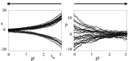
Figure 1: Simulation showing solutions of (2) and (3) for the system prepared in $|\psi_{sup}\rangle$, as approximated by (LABEL:eq:Qsqsup). The amplified $x$ propagates backwards, the $\xi_{1}(t)$ sampled from (4). The deamplified $p$ propagates forwards. $x_{1}=-x_{2}=0.8$, $r=2$.

The cause-and-effect relations for the measurement can be deduced by tracking the amplitudes in the simulation. There is a mapping of the Gaussian with mean $x_{j}$ in (LABEL:eq:Qsqsup) to a Gaussian with amplified mean $Gx_{j}$ in (4). While the eigenvalue $x_{j}$ amplifies, the noise does not. This is clarified by writing (2) as two equations, substituting $x(t)=x_{j}(t)+\delta x(t)$. The $x_{j}(t)$ is the observable part of $x$ that can be measured, given by $\frac{dx_{j}}{dt}=-gx_{j}$, which has a causal, deterministic solution, $x_{j}(t)=x_{j}(0)e^{gt}$. This gives the forward (blue) relation in Figure 2. The other part to $x(t)$ is retrocausal and stochastic: $\frac{d(\delta x)}{dt_{-}}=-g(\delta x)+\xi_{1}(t)$. The solutions give a constant average noise magnitude for $\delta x$ throughout the dynamics, as observed in Figures 1 and 2. The causal structure combines “hidden” microscopic retrocausal relations for amplitudes that are not observed, with causal relations for the amplitudes observable at a macroscopic level (Figure 2). The solutions for the forward-propagating amplitude $p$ depend on the initial boundary condition, with $p$ decaying to the vacuum noise level, $\sigma_{p}\rightarrow 1$ (Figure 1).

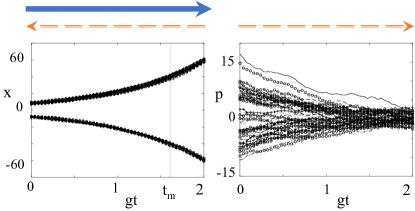
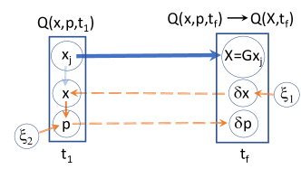
Figure 2: Top left: As for Figure 1, but $x_{1}=-x_{2}=2$ depicting a macroscopic superposition. Top right: The forward-propagating trajectories for $p$ conditioned on the positive outcome $x_{1}$ at $t_{f}$, showing fringes. Lower: The causal structure showing macroscopic forward causal relations (blue solid line) and microscopic “hidden” causal loops (red dashed lines).

There is a connection between trajectories for $x$ and $p$, determined by the conditional $Q(p|x)$ at $t_{1}=0$. We find

$$Q(p|x,t_{1}) = \frac{e^{-p^{2}/2\sigma_{p}^{2}}}{\sigma_{p}\sqrt{2\pi}}\{1-\frac{\sin(2px_{1}/\sigma_{x}^{2})}{\cosh(2xx_{1}/\sigma_{x}^{2})}\}.$$ (5)

For each backward trajectory, $x(t_{f})$ propagates back to a unique value $x(t_{1})$ at $t_{1}=0$. A distribution of $p$ values connected with $x(t_{1})$ is generated by $Q(p|x(t_{1}))$. Each such $p$ propagates forward to a value $p(t_{f})$ (Figure 2). This gives a partial causal loop, indicated by the relation at $t_{1}$, connecting $p$ from $x$. The relation requires $\mathcal{I\neq}0$. Hence, there is no such loop for $\rho_{mix}$. This establishes the link between a causal loop and a superposition.

Causal consistency demands that the joint probability density for $x$ and $p$ created from the forward and backward amplitudes at time $t$ ($t_{1}\leq t\leq t_{f}$) is given by $Q(x,p,t)$ (deutsch-1991, ). This is proved and confirmed by statistical comparisons (companion-paper, ). The correct $Q(x|p,t_{f})$ is established, to complete the loop, although $x$ and $p$ decorrelate for $t_{f}\rightarrow\infty$. The paradox that $Q$ is a function only of the time $t$ in the forward direction, and not the time $t_{f}-t$, is resolved by the causal model (Figure 2), since the retrocausal noise term $\xi_{1}$ has a magnitude independent of $t_{f}$.

The probability density of the amplitudes $x(t_{f})$ is the probability $P(x)=|\langle\psi_{sup}|x\rangle|^{2}$ for detecting the value $x(t_{f})/G$, satisfying Born’s rule as $G\rightarrow\infty$. This is because the eigenvalue $x_{j}$ amplifies to $Gx_{j}$, whereas $\delta x$ and $\mathcal{I}$ do not amplify, and the Gaussian term for $Gx_{j}$ of the marginal (4) is proportional to $|c_{j}|^{2}$. Hence, as $G\rightarrow\infty$, the trajectory value gives the value of the detected outcome. The outcome inferred for $\hat{x}$, based on a readout taking into account the amplification, is $\widetilde{x}(t_{f})=x(t_{f})/G$, which as $G\rightarrow\infty$ is one of the eigenvalues $x_{j}$ (Figure 1).

This leads to conclusions about macroscopic realism. For macroscopic superpositions $|\psi_{sup}\rangle$ ($|x_{1}-x_{2}|\gg 1$), the trajectories appear as a “line” connecting $x_{j}$ at time $t_{1}$ to $Gx_{j}$ at time $t_{f}$, with thickness $\delta x$ (the hidden vacuum noise level) (Figure 2). The final outcome can be deduced from the value of $x$ at time $t_{1}$. In fact, any $|\psi_{sup}\rangle$ becomes a macroscopic superposition, with sufficient amplification $G$ (Figure 1 at $t_{m}$). At time $t_{m}$, the scaled amplitude $\widetilde{x}(t_{m})=x(t_{m})/G$ is the outcome of the measurement $\hat{x}$. The $\widetilde{x}(t_{m})$ is not a single trajectory value, but a band of amplitudes of width $\delta x/G$, so that $\widetilde{x}(t_{m})$ is more precise as $G\rightarrow\infty$. The noise $\delta x$ in $x(t_{m})$ from the future boundary condition does not impact the present reality, defined by $\widetilde{x}(t_{m})$, for $|\psi_{sup}(t_{m})\rangle$. Consider the system in the amplified state $|\psi_{sup}(t_{m})\rangle=e^{-iHt_{m}/\hbar}|\psi_{sup}\rangle$. Prior to a measurement of $\hat{x}$, the system has a predetermined outcome $\widetilde{\lambda}_{x}=\widetilde{x}(t_{m})$ for $\hat{x}$. Recalling the definition in the introduction (leggett-1985, ), we see that macroscopic realism emerges, with sufficient amplification $G$.

Now we examine the EPR paradox (epr-1935, ). Two separated modes $A$ and $B$ prepared in a two-mode squeezed state $|\psi_{epr}\rangle=(1-\eta^{2})^{1/2}\sum_{n=0}^{\infty}\tanh^{n}r\thinspace|n\rangle_{A}|n\rangle_{B}$ at time $t_{0}$ possess EPR correlations (reid-1989, ; epr-rmp, ). Here $\eta=\tanh r$ and $|n\rangle_{A/B}$ are number states. Boson operators $\hat{a}$, $\hat{b}$ and quadrature phase amplitudes $\hat{x}_{A}$, $\hat{p}_{A}$, $\hat{x}_{B}$ and $\hat{p}_{B}$ are defined for each mode. The $Q$ function is

$$Q(\bm{\lambda},t_{0}) = \frac{(1-\eta^{2})}{\pi^{2}}e^{-\frac{1}{2}(x_{A}-x_{B})^{2}(1+\eta)}e^{-\frac{1}{2}(p_{A}+p_{B})^{2}(1+\eta)}$$ (6)

$$\times e^{-\frac{1}{2}(x_{A}+x_{B})^{2}(1-\eta)}e^{-\frac{1}{2}(p_{A}-p_{B})^{2}(1-\eta)}$$

where $\bm{\lambda}=(x_{A},x_{B},p_{A},p_{B})$. As $r\rightarrow\infty$, $|\psi_{epr}\rangle$ is an eigenstate of $\hat{x}_{A}-\hat{x}_{B}$ and $\hat{p}_{A}+\hat{p}_{B}$ (epr-1935, ). A measurement of $\hat{x}_{A}$ or $\hat{p}_{A}$ is made using $H_{A}=i\hbar ge^{2i\theta}(\hat{a}^{\dagger 2}-\hat{a}^{2})/2$ with $\theta=0$ or $\pi/2$ respectively. Similarly, $H_{B}=i\hbar ge^{2i\phi}(\hat{b}^{\dagger 2}-\hat{b}^{2})/2$ with $\phi=0$ or $\pi/2$ allows measurement of $\hat{x}_{B}$ or $\hat{p}_{B}$. The equations for measurements $\hat{x}_{A}$ and $\hat{x}_{B}$ are $\frac{dx_{K}}{dt_{-}}=-gx_{K}+\xi_{1K}\left(t\right)$ and $\frac{dp_{K}}{dt}=-gp_{K}+\xi_{2K}\left(t\right)$. The noises satisfy $\left\langle\xi_{\mu K}\left(t\right)\xi_{\nu K}\left(t^{\prime}\right)\right\rangle=2g\delta_{\mu\nu}\delta\left(t-t^{\prime}\right)$, the noise for $A$ and $B$ being independent. Transforming to $x_{\pm}=x_{A}\pm x_{B}$, $p_{\pm}=p_{A}\pm p_{B}$, the boundary condition for the backward trajectories is determined by the marginal

$$Q(x_{+},x_{-},t_{f}) = \frac{e^{-x_{-}^{2}/2\sigma_{-}^{2}(t_{f})}e^{-x_{+}^{2}/2\sigma_{+}^{2}(t_{f})}}{2\pi\sigma_{+}(t_{f})\sigma_{-}(t_{f})}$$ (7)

where $\sigma_{\pm}^{2}\left(t\right)=2(1+e^{2gt}e^{\pm 2r})$. The equations for measurements of $\hat{p}_{A}$ and $\hat{p}_{B}$ are $\frac{dp_{K}}{dt_{-}}=-gp_{K}+\xi_{1K}\left(t\right)$ and $\frac{dx_{K}}{dt}=-gx_{K}+\xi_{2K}\left(t\right)$. The solutions are identical with $p_{\pm}$ replacing $x_{\mp}$, the marginal being $Q(p_{-},p_{+},t_{f})$.

As before, macroscopic realism emerges as the system amplifies. Considering Figure 3, the outcome inferred for $\hat{x}_{A}$ at time $t_{m}$ is $\widetilde{x}_{A}(t_{m})=x_{A}(t_{m})/G$, which becomes sharp for large $G$. Hence, we identify a variable $\widetilde{\lambda}_{x}^{A}=\widetilde{x}_{A}(t_{m})$ which predetermines the outcome of a measurement $\hat{x}_{A}$ on the amplified state $e^{-iH_{A}t/\hbar}e^{-iH_{B}t/\hbar}|\psi_{epr}\rangle$ at $t=t_{m}$. For large $r$, the correlation between $\widetilde{x}_{A}(t_{m})$ and $\widetilde{x}_{B}(t_{m})$ becomes perfect, so that the outcome for $\hat{x}_{A}$ can be inferred from the measurement $\hat{x}_{B}$. Similarly, after sufficient amplification at time $t_{m}$, the outcome for $\hat{p}_{B}$ is given by $\widetilde{\lambda}_{p}^{B}=\widetilde{p}_{B}(t_{m})=p_{B}(t_{m})/G$. For $r\rightarrow\infty$, there is perfect anticorrelation between $\widetilde{p}_{A}(t)$ and $\widetilde{p}_{B}(t)$, so that the outcome for $\hat{p}_{A}$ can be inferred from $\hat{p}_{B}$.

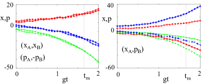
Figure 3: Left: Simulation for measurements $\hat{x}_{A}$ and $\hat{x}_{B}$ on the system $|\psi_{epr}\rangle$ where $r=2$. The paired trajectories $(x_{A},x_{B})$ corresponding to the same run are shown with the same colour/ symbol. The paired trajectories $(p_{A},-p_{B}$) for measurements $\hat{p}_{A}$ and $-\hat{p}_{B}$ are given similarly. Right: Paired trajectories $(x_{A},p_{B})$ for measurements $\hat{x}_{A}$ and $\hat{p}_{B}$. The $x_{A}$ ($p_{B}$) is given by the solid (dashed) line.

We also simulate the paradox where $\hat{x}_{A}$ and $\hat{p}_{B}$ are measured (Figure 3, right). Here, Schrödinger argued, $\hat{x}_{A}$ and $\hat{p}_{A}$ are simultaneously measured, “one by direct, the other by indirect measurement” (schrodinger-1935, ; sch-epr-exp-atom, ). Schrödinger asked whether precise predetermined values for both outcomes could exist consistently with quantum mechanics. Consider the state $e^{-iH_{A}t_{m}/\hbar}e^{-iH_{B}t_{m}/\hbar}|\psi_{epr}\rangle$ ($\theta=0$, $\phi=\pi/2$) prepared at time $t_{m}$ after amplification of $\hat{x}_{A}$ and $\hat{p}_{B}$. Consider in the simulation a given run e.g. the two lines in red at time $t_{m}$. The values given by $\widetilde{\lambda}_{x}^{A}=\widetilde{x}_{A}(t_{m})$ and $\widetilde{\lambda}_{p}^{B}=\widetilde{p}_{B}(t_{m})$ are the outcomes of $\hat{x}_{A}$ and $\hat{p}_{B}$, in that run. The value $\widetilde{\lambda}_{p,inf}^{A}=-\widetilde{\lambda}_{p}^{B}$ inferred from $B$ gives the prediction for $\hat{p}_{A}$. Experimentally, the prediction for $\hat{p}_{A}$ can be verified, by performing the unitary interaction $U_{P}^{A}$ at $A$ corresponding to $H_{A}$ with $\theta=\pi/2$ to reverse the measurement $\hat{x}_{A}$, and then amplifying to measure $\hat{p}_{A}$. This is verified in the simulation: the measurement setting at $B$ is fixed at $\hat{p}_{B}$, which ensures the final boundary condition $Q(p_{+},p_{-},t_{f})$ and hence the result $-\widetilde{p}_{B}(t_{m})$ for $\hat{p}_{A}$. The $\widetilde{\lambda}_{x}^{A}$ and $\widetilde{\lambda}_{p,inf}^{A}$ are realizations of the values sought by Schrödinger.

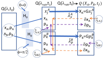
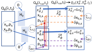
Figure 4: Causal relations associated with the simulation. Top: The system with EPR correlations as in Figure 3, right. The solid vertical arrows depict correlations due to entanglement between $A$ and $B$, leading to nonlocal loops. Lower: The system violating the Bell inequality. Local loops are apparent at both sites, as well as nonlocal loops.

The variables $\widetilde{\lambda}_{x}^{A}$, $\widetilde{\lambda}_{p,inf}^{A}$ (and similarly $\widetilde{\lambda}_{x,inf}^{B}$, $\widetilde{\lambda}_{p}^{B}$) give a simultaneous predetermination of the outcomes of measurements of $\hat{x}_{A}$ and $\hat{p}_{A}$, but do not conflict with known violations of Bell inequalities. This is because they are defined only for systems after the choice of measurement setting: $\widetilde{\lambda}_{x}^{A}$ is defined after choice $\theta=0$; $\widetilde{\lambda}_{p,inf}^{A}$ is defined after choice $\phi=\pi/2$. EPR’s local realism implies predetermined values $\lambda_{x,epr}^{A}$, $\lambda_{p,epr}^{A}$ for $\hat{x}_{A}$ and $\hat{p}_{A}$ $-$ regardless of whether the interactions determining the measurement settings have taken place. This allows multiple “elements of reality” $\lambda_{\theta,epr}^{A}$ and $\lambda_{\phi,epr}^{B}$ to be simultaneously defined for three or more settings (bohm-2012, ), leading to a Bell violation and falsification of local realism (bell-1964, ).

The simulations reveal consistency with a restricted form of local realism (refer (thenabadu-2022, ; philippe-grang-context, ; bell-2004, )). Consider the EPR system with measurement settings $\theta$ and $\phi$ prepared at time $t_{m}$, via amplification, for a readout of outcomes in the future. The associated variables $\widetilde{\lambda}_{\theta}^{A}$ and $\widetilde{\lambda}_{\phi}^{B}$ in the simulation determine those outcomes. The future boundary condition ensures that $\widetilde{\lambda}_{\theta}^{A}$ is the outcome at $A$ independently of any changes of setting $\phi$ at $B$ $-$ provided the setting $\theta$ at $A$ is fixed. This defines a weak form of local realism: the outcome of the measurement is predetermined once the local measurement setting is fixed (by amplification), and there is no disturbance to that value by any change of measurement setting at $B$. Similarly, we see from the boundary conditions of the simulation that the prediction $\widetilde{\lambda}_{\phi,inf}^{A}$ inferred from $B$ for the measurement given by the setting $\phi$ at $A$ is valid, independently of any change of $\theta$ at $A$, provided $\phi$ is fixed.

On the other hand, realization of the prediction for $A$ requires a further unitary interaction $U_{\phi}^{A}$ at $A$. If the setting $\phi$ is changed at $B$ (via a local unitary interaction $U^{B}$), then the boundary condition in the simulation changes. Over both unitary interactions, we cannot validate the full EPR local-realism premise, that the inferred prediction $\widetilde{\lambda}_{\phi,inf}^{A}\equiv\lambda_{\phi,epr}^{A}$ for $A$ is a property retained for that system, independent of $\phi$ at $B$.

We now examine violations of Bell inequalities (Figure 4). The partial relaxation of EPR’s local-realism, consistent with the variables $\widetilde{\lambda}_{\theta}^{A}$, $\widetilde{\lambda}_{\phi}^{B}$ that determine a real property for the amplified system, is sufficient to allow violations. We consider measurements of rotated quadratures $\hat{x}_{\theta,A}=\hat{x}_{A}\cos\theta+\hat{p}_{A}\sin\theta$ and $\hat{x}_{\phi,B}=\hat{x}_{B}\cos\phi+\hat{p}_{B}\sin\phi$ on modes prepared in a state $|\psi_{B}\rangle$ with $Q$ function $Q_{B}(\bm{\lambda},t_{0})$. The outcomes are binned according to sign to give $\pm 1$. For certain $|\psi_{B}\rangle$, it is known that a Bell inequality is violated (gilchrist-prl-bell, ). The simulation begins with the choice of settings $\theta$ and $\phi$. Interactions $H_{\theta/\phi}=\hbar\kappa\hat{n}_{A/B}$ provide phase shifts that determine $\theta$, $\phi$. These give deterministic causal relations: $x_{\theta,A}=x_{A}\cos\theta+p_{A}\sin\theta$, $p_{\theta,A}=-x_{A}\sin\theta+p_{A}\cos\theta$ where $\theta=|\kappa|t$, and similarly at $B$ (thin blue lines in Figure 4). The evolved $Q$ function is $Q_{B}(\bm{\lambda_{rot}},t_{1})$ where $\bm{\lambda_{rot}}=(x_{\theta,A},p_{\theta,A},x_{\phi,B},p_{\phi,B})$. The $\hat{x}_{\theta,A}$ and $\hat{x}_{\phi,B}$ are then amplified at each site, the dynamical equations being identical to those for measurement of $\hat{x}_{A}$ and $\hat{x}_{B}$ on the EPR state, but replacing $\bm{\lambda}$ with $\bm{\lambda_{rot}}$. The density of amplitudes $x_{\theta,A}$, $x_{\phi,B}$ as $G\rightarrow\infty$ coincides with the probabilities of outcomes for $|\psi_{B}\rangle$, which violate a Bell inequality.

Bell’s local causality condition is $P(++|\theta,\phi)=\int d\lambda\rho(\lambda)P_{A}(+|\lambda,\theta)P_{B}(+|\lambda,\phi)$ where $P(++|\theta,\phi)$ is the probability of obtaining $+1$ at both sites with settings $\theta$ and $\phi$; $\rho(\lambda)$ is the distribution for hidden variables $\lambda$, and $P_{A}(+|\lambda,\theta)$ ($P_{B}(+|\lambda,\phi)$) is the probability for $+1$ at $A$ ($B$), given $\lambda$ and $\theta$ ($\phi)$ (bell-2004, ; clauser-shimony-1978, ). The interactions $H_{\theta/\phi}$ are local and the amplitudes $x_{\theta,A}$, $x_{\phi,B}$ if measurable would lead to moments satisfying Bell’s condition, with $\rho(\lambda)\equiv Q_{B}(\bm{\lambda},t_{0})$. However, over both rotations (noting $\theta,\phi\neq 0$), the unobservable $\mathcal{I}$ in $Q_{B}(\bm{\lambda},t_{0})$ contribute to observable probabilities in $Q_{B}(\bm{\lambda_{rot}},t_{1})$ (and vice versa) and the condition fails. From Figure 4, we see there is indeed no causal relation from $x_{\theta,A}$ at $t_{1}$ to a value at $t_{f}$ that depends only on $\bm{\lambda}$ and $\theta$. The solutions reveal hidden causal loops, connecting variables both locally and nonlocally, the backward-propagating amplitudes creating a discontinuity at $t_{1}$. The forward relation for the eigenvalue $x_{\theta,j}^{A}$ (solid blue line) leads to the variable $\widetilde{\lambda}_{\theta}^{A}$, but corresponds to a band of amplitudes, and is subject to $Q_{B}(\bm{\lambda_{rot}},t_{1})$ which depends on both settings. There is no nonlocal influence between $A$ and $B$ after $t_{0}$, the vertical lines connecting $A$ and $B$ representing correlations due to entanglement, quantifiable by $Q_{B}$.

References

• (1) J. S. Bell, Physics 1, 195 (1964).
• (2) J. S. Bell, Speakable and unspeakable in quantum mechanics: Collected papers on quantum philosophy (Cambridge University Press, 2004).
• (3) J. F. Clauser and A. Shimony, Rep. Prog. Phys. 41, 1881 (1978). N. Brunner et al, Rev. Mod. Phys. 86, 419 (2014).
• (4) P. H. Eberhard and R. R. Ross, Found. Phys. Lett. 2, 127 (1989).
• (5) J. A. Wheeler, in Mathematical foundations of quantum theory (Elsevier, 1978) pp. 9–48.
• (6) D. Pegg, Phys. Lett. A 78, 233 (1980).
• (7) J. G. Cramer, Phys. Rev. D 22, 362 (1980).
• (8) Y. Aharonov et al, Phys. Rev. 134, B1410 (1964).
• (9) M. AraΓΊjo, C. Branciard, F. Costa, A. Feix, C. Giarmatzi, Č. Brukner, New Journ. Phys. 17, 102001 (2015).
• (10) J. Barrett, R. Lorenz, and O. Oreshkov, Nature communications 12, 1 (2021).
• (11) J.-M. A. Allen, J. Barrett, D. C. Horsman, C. M. Lee, and R. W. Spekkens, Phys. Rev. X 7, 031021 (2017).
• (12) K. B. Wharton and N. Argaman, Rev. Mod. Phys. 92, 021002 (2020).
• (13) H. Price, Studies in History and Philosophy of Modern Physics 39, 752 (2008).
• (14) M. O. Scully and K. DrΓΌhl, Phys. Rev. A 25, 2208 (1982).
• (15) R. Chaves, G. B. Lemos and J. Pienaar, Phys. Rev. Lett. 120, 190401 (2018).
• (16) C. Giarmatzi, in Rethinking Causality in Quantum Mechanics (Springer, 2019) pp. 125–150.
• (17) F. Costa and S. Shrapnel, New J. Phys. 18, 063032 (2016). S. Shrapnel, The British Journal for the Philosophy of Science 70, 1 (2019).
• (18) P. Drummond, Phys. Rev. Research 3, 013240 (2021).
• (19) M. Hall and C. Branciard, Phys. Rev. A 102, 052228 (2020).
• (20) S. Hossenfelder and T. Palmer, Front. Phys. 8, 139 (2020).
• (21) D. Bohm, Phys. Rev. 85, 166 (1952).
• (22) W. Struyve, Rep. Prog. Phys. 73, 106001 (2010).
• (23) V. Scarani, J.-D. Bancal, A. Suarez, and N. Gisin, Found. Phys. 44, 523 (2014).
• (24) C. J. Wood and R. W. Spekkens, New J. Phys. 17, 033002 (2015).
• (25) E. G. Cavalcanti, Phys. Rev. X 8, 021018 (2018).
• (26) J. Pearl and E. G. Cavalcanti, Quantum 5, 518 (2021).
• (27) G. Castagnoli, Phys. Rev. A 104, 032203 (2021).
• (28) V. Vilasini and R. Colbeck, Phys. Rev. A 106, 032204 (2022); Phys. Rev. Lett. 129, 110401 (2022).
• (29) A. Einstein, B. Podolsky, and N. Rosen, Phys. Rev. 47, 777 (1935).
• (30) A. Leggett and A. Garg, Phys. Rev. Lett. 54, 857 (1985).
• (31) See companion paper for further details and proofs. arXiv 2205.06070Β [quant-ph].
• (32) P. D. Drummond and M. D. Reid, Phys. Rev. Research 2, 033266 (2020); Entropy 23, 749 (2021).
• (33) S. Friederich, The British Journal for the Philosophy of Science, 0, ja (2021), pp null. arXiv 2106.13502 (2021).
• (34) H. P. Yuen, Phys. Rev. A 13, 2226 (1976).
• (35) K. Husimi, Proc. Phys. Math. Soc. Jpn. 22, 264 (1940).
• (36) Similar to the consistency observed in: D. Deutsch, Phys. Rev. D 44, 3197 (1991). J. A. Wheeler and R. Feynman, Rev. Mod. Phys. 17, 157 (1945); 21, 425 (1949).
• (37) M. D. Reid, Phys. Rev. A 40, 913 (1989).
• (38) M. D. Reid et al, Rev. Mod. Phys. 81, 1727 (2009).
• (39) E. SchrΓΆdinger, Naturwissenschaften 23, 844-849 (1935).
• (40) P. Colciaghi, Y. Li, P. Treutlein, and T. Zibold, arXiv:2211.05101v1.
• (41) D. Bohm, Quantum Theory (Prentice-Hall, New York, 1951).
• (42) For similar weak versions of realism see: M. Thenabadu and M. D. Reid, Phys. Rev. A 105, 052207 (2022); Phys. Rev. A 105, 062209 (2022). J. Fulton et al, arXiv:2208.01225, R. Joseph et al, arXiv 2211.02877. See also Bell’s description of ’beables’ in [2] and [43].
• (43) P. Grangier, Entropy 23, 1660 (2021).
• (44) U. Leonhardt and J. Vaccaro, Journ. Mod. Opt. 42, 939 (1995). A. Gilchrist, P. Deuar and M. D. Reid, Phys. Rev. Lett. 80, 3169 (1998); Phys. Rev. A 60, 4259 (1999).