Self-Asymmetric Invertible Network for Compression-Aware Image Rescaling

Abstract

High-resolution (HR) images are usually downscaled to low-resolution (LR) ones for better display and afterward upscaled back to the original size to recover details. Recent work in image rescaling formulates downscaling and upscaling as a unified task and learns a bijective mapping between HR and LR via invertible networks. However, in real-world applications (e.g., social media), most images are compressed for transmission. Lossy compression will lead to irreversible information loss on LR images, hence damaging the inverse upscaling procedure and degrading the reconstruction accuracy. In this paper, we propose the Self-Asymmetric Invertible Network (SAIN) for compression-aware image rescaling. To tackle the distribution shift, we first develop an end-to-end asymmetric framework with two separate bijective mappings for high-quality and compressed LR images, respectively. Then, based on empirical analysis of this framework, we model the distribution of the lost information (including downscaling and compression) using isotropic Gaussian mixtures and propose the Enhanced Invertible Block to derive high-quality/compressed LR images in one forward pass. Besides, we design a set of losses to regularize the learned LR images and enhance the invertibility. Extensive experiments demonstrate the consistent improvements of SAIN across various image rescaling datasets in terms of both quantitative and qualitative evaluation under standard image compression formats (i.e., JPEG and WebP). Code is available at https://github.com/yang-jin-hai/SAIN.

1 Introduction

Figure 1: Image rescaling without or with compression.

Figure 2: Illustration and empirical analysis of the Dual-IRN baseline under the proposed asymmetric framework. The early-layer features of the U-IRN exhibit high similarity to the final output of the D-IRN (i.e., the high-quality LR images). Besides, the latent variables of the U-IRN generally have a multi-modal distribution. Our SAIN model is inspired by these phenomena.

With advances in computational photography and imaging devices, we are facing increasing amounts of high-resolution (HR) visual content nowadays. For better display and storage saving, HR images are often downscaled to low-resolution (LR) counterparts with similar visual appearances. The inverse upscaling is hence indispensable to recover LR images to the original sizes and restore the details. Super-resolution algorithms (Dong et al. 2015; Dai et al. 2019) have been the prevalent solution to increase image resolution, but they commonly assume the downscaling operator is pre-determined and not learnable. To enhance the reconstruction quality, recent works (Kim et al. 2018; Xiao et al. 2020; Guo et al. 2022) have attempted to jointly optimize the downscaling and upscaling process. Especially, IRN (Xiao et al. 2020) firstly model the conversion between HR and LR image pairs as a bijective mapping with invertible neural networks (INN) to preserve as much information as possible and force the high-frequency split to follow a case-agnostic normal distribution, as shown in Fig. 1(a).

However, the LR images are usually compressed (Son et al. 2021) to further reduce the bandwidth and storage in realistic scenarios, especially for transmission on social media with massive users. Worse still, lossy compression (e.g. JPEG and WebP) has become a preference for social networks and websites. Although standard image compression formats (Wallace 1992; Google 2010) take advantage of human visual characteristics and thus produce visually-similar contents, they still lead to inevitable additional information loss, as shown in Fig. 1(b). Due to the bijective nature, the INN-based approaches (Xiao et al. 2020; Liang et al. 2021) perform symmetric rescaling and thus are especially sensitive to the distribution shift caused by these compression artifacts. In this sense, lossy compression can also be utilized as an adversarial attack to poison the upscaling procedure.

In this paper, we tackle compression-aware image rescaling via a Self-Asymmetric Invertible Network (SAIN). Before delving into the details, we start with empirical analyses of a baseline model Dual-IRN. To mitigate the influence of compression artifacts, we instantiate the Dual-IRN with an asymmetric framework, establishing two separate bijective mappings, as shown in Fig. 2(a). Under this framework, we can conduct downscaling with the D-IRN to derive visually-pleasing LR images and then, after compression distortion, use the U-IRN for compression-aware upscaling. To study the behavioral difference between the two branches, we adopt the CKA metric (Kornblith et al. 2019) to measure the representation similarity. As shown in Fig. 2(b), the obtained high-quality LR images (i.e., the final outputs of D-IRN) are highly similar to the anterior-layer features of the U-IRN. Besides, we plot the histograms of the high-frequency splits in Fig. 2(c), which are previously assumed to follow the normal distribution. Interestingly, this assumption does not hold for the latent variables of the compression-aware U-IRN, which exhibits a multi-modal pattern.

Inspired by the analysis above, we inject our SAIN model with inductive bias. First, we inherit the asymmetric framework from Dual-IRN, which can upscale from compression-distorted LR images without sacrificing the downscaling quality. Second, we present a compact network design with Enhanced Invertible Block and decouple the blocks into the downscaling module and the compression simulator, which enables approximating high-quality and compressed LR in one forward pass. Third, we adopt isotropic Gaussian mixtures to model the joint information loss under the entangled effect of downscaling and compression.

Our main contributions are highlighted as follows:

• To our knowledge, this work is the first attempt to study image rescaling under compression distortions. The proposed SAIN model integrates rescaling and compression into one invertible process with decoupled modeling.

• We present a self-asymmetric framework with Enhanced Invertible Block and design a series of losses to enhance the reconstruction quality and regularize the LR features.

• Both quantitative and qualitative results show that SAIN outperforms state-of-the-art approaches by large margins under standard image codecs (i.e., JPEG and WebP).

2 Related Work

Invertible Neural Networks. Invertible neural networks (INNs) originate from flow-based generative models (Dinh, Krueger, and Bengio 2014; Dinh, Sohl-Dickstein, and Bengio 2016). With careful mathematical designs, INNs learn a bijective mapping between the source domain and the target domain with guaranteed invertibility. Normalizing-flow methods (Rezende and Mohamed 2015; Kobyzev, Prince, and Brubaker 2020) map a high-dimensional distribution (e.g. images) to a simple latent distribution (e.g., Gaussian). The invertible transformation allows for tractable Jacobian determinant computation, so the posterior probabilities can be explicitly derived and optimized by maximum likelihood estimation (MLE). Recent works have applied INNs to different visual tasks, including super-resolution (Lugmayr et al. 2020) and image rescaling (Xiao et al. 2020).

Image Rescaling. Super-resolution (SR) (Dong et al. 2015; Lim et al. 2017; Zhang et al. 2018b) aims to reconstruct the HR image given the pre-downscaled one. Traditional image downscaling usually adopts low-pass kernels (e.g., Bicubic) for interpolation sub-sampling, which generates over-smoothed LR images due to high-frequency information loss. Differently, image rescaling (Kim et al. 2018; Li et al. 2018; Sun and Chen 2020) jointly optimize downscaling and upscaling as a unified task in an encoder-decoder paradigm. IRN (Xiao et al. 2020) models image rescaling as a bijective transformation with INN to maintain as much information about the HR images. The residual high-frequency components are embedded into a case-agnostic latent distribution for efficient reconstruction. Recently, HCFlow (Liang et al. 2021) proposes a hierarchical conditional flow to unify image SR and image rescaling tasks in one framework.

However, image downscaling is often accompanied by image compression in applications. Although flow-based methods perform well in ideal image rescaling, they are vulnerable to lossy compression due to the high reliance on reversibility. A subtle interference on the LR images usually causes a considerable performance drop.

Figure 3: Overview of the proposed Self-Asymmetric Invertible Network (SAIN). We decouple the invertible architecture into the downscaling module $f$ to generate visually-appealing LR images and the compression simulator $g$ to mimic standard codecs. Thus, due to the reversible nature of InvBlocks, we can inversely restore the compression distortion via $g^{-1}$ from LR images that are compressed by real codecs (albeit not perfectly), and then upscale to original size via $f^{-1}$. The $\exp(\cdot)$ of $\rho$ is omitted.

3 Methodology

3.1 Preliminaries

Normalizing flow models (Kobyzev, Prince, and Brubaker 2020) usually propagate high-dimensional distribution (e.g. images) through invertible transformation to enforce a simple specified distribution. The Jacobian determinant of such invertible transformation is easy to compute so that we can inversely capture the explicit distribution of input data and minimize the negative log-likelihood in the source domain.

In the image rescaling task, however, the target domain is the LR images, whose distribution is implicit. Therefore, IRN (Xiao et al. 2020) proposes to split HR images $x$ into low-frequency and high-frequency components $[x_{l},x_{h}]$ and learn the invertible mapping $[x_{l},x_{h}]\leftrightarrow[y,a]$, where $y$ is the desired LR image and $a\sim\mathcal{N}(0,1)$ is case-agnostic.

In this work, we establish an asymmetric framework to enhance the robustness against image compression for the rescaling task. In the forward approximation pass, we not only model the downscaling process by $f$ but also simulate the compressor by $g$. The downscaling module $f$ alone can derive the visually-pleasing LR $y$, while the function composition $f\circ g$ maps $[x_{l},x_{h}]\rightarrow[\hat{y},\hat{z}]$, where $\hat{y}$ is the simulated compressed LR. When $y$ suffers from compression distortion $\varepsilon$ and results in $y^{\prime}$, the reverse restoration pass is used to reconstruct the HR contents by $[y^{\prime},z]\rightarrow x^{\prime}$. The forward and inverse pass are asymmetric but share one invertible structure. The ultimate goal is to let $x^{\prime}$ approach the true HR $x$.

3.2 Self-Asymmetric Invertible Network

The difficulty of compression-robust image rescaling lies in designing a model that performs both high-quality downscaling and compression-distorted upscaling. Since we approximate the downscaling and the compression process in one forward pass, and they essentially share large proportions of computations, it is important to avoid confusion in the low-frequency split. In this work, we assume that the information loss caused by compression is conditional on the high-frequency components, and thus devise the Enhanced Invertible Block (E-InvBlock). During upscaling, the latent variable $z$ is sampled from a learnable Gaussian mixture to help recover details from perturbed LR images. The overall framework is illustrated in Fig. 3.

Haar Transformation.

We follow existing works (Xiao et al. 2020; Liang et al. 2021) to split the input image via the Haar transformation. This channel splitting is crucial for the construction of invertible modules (Kingma and Dhariwal 2018; Ho et al. 2019). Haar transformation decomposes an image into a low-pass approximation, the horizontal, vertical, and diagonal high-frequency coefficients (Lienhart and Maydt 2002). The low-frequency (LF) approximation and the high-frequency (HF) components represent the input image as $[x_{l},x_{h}]$. For a scale larger than 2, we adopt successive Haar transformations to split the channels at the first.

Vanilla Invertible Block.

The Vanilla Invertible Block (V-InvBlock) inherits the design in IRN (Xiao et al. 2020). It is a rearrangement of existing coupling layers (Dinh, Krueger, and Bengio 2014; Dinh, Sohl-Dickstein, and Bengio 2016) to fit the image rescaling task. For the $j$-th layer,

$$x_{l}^{j+1} =x_{l}^{j}+\phi\left(x_{h}^{j}\right)~{},$$ (1)

$$x_{h}^{j+1} =x_{h}^{j}\odot\exp\left(\rho\left(x_{l}^{j+1}\right)\right)+\eta\left(x_{l}^{j+1}\right)~{},$$ (2)

where $\odot$ denotes the Hadamard product and in practice, we use a centered Sigmoid function for numerical stability after the exponentiation. The inverse step is easily obtained by

$$x_{h}^{j} =\left(x_{h}^{j+1}-\eta\left(x_{l}^{j+1}\right)\right)\odot\exp\left(-\rho\left(x_{l}^{j+1}\right)\right)~{},$$ (3)

$$x_{l}^{j} =x_{l}^{j+1}-\phi\left(x_{h}^{j}\right)~{}.$$ (4)

Enhanced Invertible Block.

In V-InvBlock, the LF part is polished by a shortcut connection on the HF branch. Since $f$ is cascaded to $g$, simply repeating the V-InvBlock to construct $f$ would cause ambiguity in the LF branch. Therefore, we augment the LF branch and thus make the modeling of the high-quality LR $y$ and the emulated compressed LR $\hat{y}$ separable to some extent. Generally, we let $x_{l}$ help stimulate $\hat{y}$, and let the intermediate representation $y_{i}$ undertake the polishing for $y$. Since there is no information loss inside the block, we assume the compression distortion can be recovered from the HF components. Formally,

$$y_{i} =x_{l}^{i}+\phi\left(x_{h}^{i}\right)~{},$$ (5)

$$x_{l}^{i+1} =y_{i}-\varphi\left(x_{h}^{i}\right)~{}.$$ (6)

It only brings a slight increase in computational overhead but significantly increases the model capacity. Note that $\phi(\cdot)$, $\varphi(\cdot)$, $\eta(\cdot)$, and $\rho(\cdot)$ can be arbitrary functions.

Isotropic Gaussian Mixture.

The case-specific information is expected to be completely embedded into the downscaled image, since preserving the HF components is impractical. IRN (Xiao et al. 2020) forces the case-agnostic HF components to follow $N(0,I)$ and sample from the same distribution for inverse upscaling. However, due to the mismatch between real compression and simulated compression, the distribution of the forwarded latent $\hat{z}$ and the underlying upscaling-optimal latent $z$ are arguably not identical. Besides, as shown in Fig. 2(c), the latent distribution of the compression-aware branch presents a multimodal pattern. Therefore, rather than explicitly modeling the distribution of $\hat{z}$, we choose to optimize a learnable Gaussian mixture to sample for upscaling from compressed LR images. For simplicity, we assume the Gaussian mixture is isotopic (Améndola, Engström, and Haase 2020) and all dimensions of $z$ follow the same univariate marginal distribution. For any $z_{o}\in z$:

$$p(z_{o})=\sum_{k=1}^{K}\pi_{k}\mathcal{N}\left(z_{o}\mid\mu_{k},\sigma_{k}\right)~{},$$ (7)

where the mixture weights $\pi_{k}$, means $\mu_{k}$, and variances $\sigma_{k}$ are learned globally. Since the sampling operation is non-differentiable, enabling end-to-end optimization of the parameters $\{\pi_{k},\mu_{k},\sigma_{k}\}$ is non-trivial. We decompose the sampling from $p(z_{o})$ into two independent steps: (1) discrete sampling $k\sim\text{Categorical}(\pi)$ to select a component; (2) sample $z_{o}$ from the parameterized $\mathcal{N}(\mu_{k},\sigma_{k})$. In this way, we use Gumbel-Softmax (Jang, Gu, and Poole 2017) to approximate the first step and use the reparameterization trick (Kingma and Welling 2013) for the second step, and thus estimate the gradient for backpropagation.

Compression and Quantization.

To jointly optimize the upscaling and the downscaling steps under compression artifacts, we employ a differentiable JPEG simulator (Xing, Qian, and Chen 2021) to serve as a virtual codec $\varepsilon$. It performs discrete cosine transform on each 8$\times$8 block of an image and simulates the rounding function with the Fourier series. For the LR and HR images, we use the Straight-Through Estimator (Bengio, Léonard, and Courville 2013) to calculate the gradients of the quantization module. Moreover, we incorporate real compression distortion $\epsilon$ to provide guidance for network optimization, which extends our model to be also suitable for other image compression formats besides JPEG.

3.3 Training Objectives

The downscaling module, the compression simulator, and the inverse restoration procedure are jointly optimized. The overall loss function is a linear combination of the final reconstruction loss and a set of LR guidance to produce visually-attractive LR images and meanwhile enhance the invertibility:

$$\mathcal{L}=\lambda_{1}\mathcal{L}_{{rec}}+\lambda_{2}\mathcal{L}_{fit}+\lambda_{3}\mathcal{L}^{\prime}_{{fit}}+\lambda_{4}\mathcal{L}_{{reg}}+\lambda_{5}\mathcal{L}_{{rel}}~{}.$$ (8)

HR Reconstruction.

Despite the information loss caused by the downscaling and the compression, we expect that given a model-downscaled LR $y$, the counterpart HR image $x$ can be restored by our model using a random sample of $z$ from the learned distribution $p(z_{o})$:

$$\mathcal{L}_{rec}=\mathcal{L}_{hr}\left(f^{-1}\left(g^{-1}\left(\left[y,z\right]\right)\right),x\right)~{}.$$ (9)

LR Guidance.

First, the model-downscaled LR images should be visually-meaningful. We follow existing image rescaling works (Kim et al. 2018; Xiao et al. 2020) to drive the LR images $y$ to resemble Bicubic interpolated images as a guidance of the downscaling module $f$:

$$\mathcal{L}_{fit}=\mathcal{L}_{lr}\left(\operatorname{Bicubic}\left(x\right),y\right)~{}.$$ (10)

Second, to better simulate the compression distortions and the inverse restoration, we encourage the model-distorted LR image $\hat{y}$ to approximate the compressed version of the Bicubic downscaled LR image which undergoes the distortion $\epsilon$ of a real image compression process:

$$\mathcal{L}_{fit}^{\prime}=\mathcal{L}_{lr}\left(\epsilon\left(\operatorname{Bicubic\left(x\right)}\right),\hat{y}\right)~{}.$$ (11)

Third, we regularize the similarity between the model-downscaled LR image $y$ and the inversely restored LR image $y_{r}$ to enhance reversibility: $\mathcal{L}_{reg}=\mathcal{L}_{lr}\left(y,y_{r}\right)$.

Finally, we further facilitate the compression simulation by enforcing the relation between $y$ and $\hat{y}$: $\mathcal{L}_{rel}=\mathcal{L}_{lr}\left(\epsilon\left(y\right),\hat{y}\right)$. Note that $\epsilon$ can be any image compressor to make our model robust against other compression formats.

4 Experiments

Downscaling & Upscaling	Scale	JPEG QF=30	JPEG QF=50	JPEG QF=70	JPEG QF=80	JPEG QF=90
Bicubic & Bicubic	$\times 2$	29.38 / 0.8081	30.19 / 0.8339	30.91 / 0.8560	31.38 / 0.8703	31.96 / 0.8878
Bicubic & SRCNN (Dong et al. 2015)	$\times 2$	28.01 / 0.7872	28.69 / 0.8154	29.43 / 0.8419	30.01 / 0.8610	30.88 / 0.8878
Bicubic & EDSR (Lim et al. 2017)	$\times 2$	28.92 / 0.7947	29.93 / 0.8257	31.01 / 0.8546	31.91 / 0.8753	33.44 / 0.9052
Bicubic & RDN (Zhang et al. 2018b)	$\times 2$	28.95 / 0.7954	29.96 / 0.8265	31.02 / 0.8549	31.91 / 0.8752	33.41 / 0.9046
Bicubic & RCAN (Zhang et al. 2018a)	$\times 2$	28.84 / 0.7932	29.84 / 0.8245	30.94 / 0.8538	31.87 / 0.8749	33.44 / 0.9052
CAR & EDSR (Sun and Chen 2020)	$\times 2$	27.83 / 0.7602	28.66 / 0.7903	29.44 / 0.8165	30.07 / 0.8347	31.31 / 0.8648
IRN (Xiao et al. 2020)	$\times 2$	29.24 / 0.8051	30.20 / 0.8342	31.14 / 0.8604	31.86 / 0.8783	32.91 / 0.9023
SAIN (Ours)	$\times 2$	31.47 / 0.8747	33.17 / 0.9082	34.73 / 0.9296	35.46 / 0.9374	35.96 / 0.9419
Bicubic & Bicubic	$\times 4$	26.27 / 0.6945	26.81 / 0.7140	27.28 / 0.7326	27.57 / 0.7456	27.90 / 0.7618
Bicubic & SRCNN (Dong et al. 2015)	$\times 4$	25.49 / 0.6819	25.91 / 0.7012	26.30 / 0.7206	26.55 / 0.7344	26.84 / 0.7521
Bicubic & EDSR (Lim et al. 2017)	$\times 4$	25.87 / 0.6793	26.57 / 0.7052	27.31 / 0.7329	27.92 / 0.7550	28.88 / 0.7889
Bicubic & RDN (Zhang et al. 2018b)	$\times 4$	25.92 / 0.6819	26.61 / 0.7075	27.33 / 0.7343	27.92 / 0.7556	28.84 / 0.7884
Bicubic & RCAN (Zhang et al. 2018a)	$\times 4$	25.77 / 0.6772	26.45 / 0.7031	27.21 / 0.7311	27.83 / 0.7537	28.82 / 0.7884
Bicubic & RRDB (Wang et al. 2018)	$\times 4$	25.87 / 0.6803	26.58 / 0.7063	27.36 / 0.7343	27.99 / 0.7568	28.98 / 0.7915
CAR & EDSR (Sun and Chen 2020)	$\times 4$	25.25 / 0.6610	25.76 / 0.6827	26.22 / 0.7037	26.69 / 0.7214	27.91 / 0.7604
IRN (Xiao et al. 2020)	$\times 4$	25.98 / 0.6867	26.62 / 0.7096	27.24 / 0.7328	27.72 / 0.7508	28.42 / 0.7777
HCFlow (Liang et al. 2021)	$\times 4$	25.89 / 0.6838	26.38 / 0.7029	26.79 / 0.7204	27.05 / 0.7328	27.41 / 0.7485
SAIN (Ours)	$\times 4$	27.90 / 0.7745	29.05 / 0.8088	29.83 / 0.8272	30.13 / 0.8331	30.31 / 0.8367

Table 1: Quantitative results (PSNR / SSIM) of image rescaling on DIV2K under distortion at different JPEG QFs.

Figure 4: Cross-dataset evaluation of image rescaling ($\times 2$) over standard benchmarks: Set5, Set14, BSD100, and Urban100.

4.1 Experimental Setup

Datasets and Settings.

We adopt the 800 HR images from the widely-acknowledged DIV2K training set (Agustsson and Timofte 2017) to train our model. Apart from the DIV2K validation set, we also evaluate our model on 4 standard benchmarks: Set5 (Bevilacqua et al. 2012), Set14 (Zeyde, Elad, and Protter 2010), BSD100 (Martin et al. 2001), and Urban100 (Huang, Singh, and Ahuja 2015). Following the convention in image rescaling (Xiao et al. 2020; Liang et al. 2021), the evaluation metrics are Peak Signal-to-Noise Ratio (PSNR) and SSIM (Wang et al. 2004) on the Y channel of the YCbCr color space.

Implementation Details.

For $\times 2$ and $\times 4$ image rescaling, we use a total of 8 and 16 InvBlocks in total, and the downscaling module $f$ has 5 and 10 E-InvBlocks, respectively. The transformation functions $\phi(\cdot)$, $\varphi(\cdot)$, $\eta(\cdot)$, and $\rho(\cdot)$ are implemented with Dense Block (Wang et al. 2018; Xiao et al. 2020). The input images are cropped to 128$\times$128 and augmented via random horizontal and vertical flips. We adopt Adam optimizer (Kingma and Ba 2014) with $\beta_{1}=0.9$ and $\beta_{2}=0.999$, and set the mini-batch size to 16. The model is trained for 500$k$ iterations. The learning rate is initialized as $2\times 10^{-4}$ and reduced by half every $100k$ iterations. We use $\mathcal{L}_{1}$ pixel loss as the LR guidance loss $\mathcal{L}_{lr}$ and $\mathcal{L}_{2}$ pixel loss as the HR reconstruction loss. To balance the losses in LR and HR spaces, we use $\lambda_{1}=1$ and $\lambda_{2}=\lambda_{3}=\lambda_{4}=\lambda_{5}=\frac{1}{4}$. The compression quality factor (QF) is empirically fixed at 75 during training. The Gaussian mixture for upscaling has $K=5$ components.

4.2 Evaluation under JPEG Distortion

JPEG (Wallace 1992) is the most widely-used lossy image compression method in consumer electronic products. As various compression QFs may be used in applications, we expect SAIN to be a one-size-fits-all model. That is, after compression-aware training under a specific format, it can handle compression distortions at different QFs.

Figure 5: Qualitative results of image rescaling ($\times$2) on DIV2K under distortion at different JPEG QFs. Due to space limitation, we only visualize results of the top three methods at each QF. More results can be found in the supplementary material.

Quantitative Evaluation.

We compare our model with three kinds of methods: (1) Bicubic downscaling & super-resolution (Dong et al. 2015; Lim et al. 2017; Zhang et al. 2018a, b); (2) jointly-optimized downscaling and upscaling (Sun and Chen 2020); (3) flow-based invertible rescaling models (Xiao et al. 2020; Liang et al. 2021). We reproduce all the compared methods and get similar performance as claimed in their original papers when tested without compression distortions. Then, for each approach, we apply JPEG distortion to the downscaled LR images at different QFs (i.e., 30, 50, 70, 80, 90), and evaluate the construction quality of the upscaled HR images.

As is evident in Tab. 1, the proposed SAIN outperforms existing methods by a large margin at both scales and across all testing QFs. The reconstruction PSNR of SAIN significantly surpasses the second best results by 1.33-3.59 dB. The performances of previous state-of-the-arts drop severely as JPEG QF descents and are even worse than naïve Bicubic resampling at lower QF and larger scale. HCFlow (Liang et al. 2021) suffers even more from the compression artifacts than IRN (Xiao et al. 2020) since it assumes the HF components are conditional on the LF part.

Cross-Dataset Validation.

In addition to the DIV2K validation set, we further verify our methods on 4 standard benchmarks (Set5, Set14, BSD100, Urban100) to investigate the cross-dataset performance. Similarly, we test all the compared models at different QFs for the $\times 2$ image rescaling task, and plot the corresponding PSNR in Fig. 4.

From these curves, we can clearly observe that the proposed approach SAIN achieves substantial improvements over the state-of-the-arts. SRCNN (Dong et al. 2015) adopts a very shallow convolutional network to increase image resolution and thus is quite fragile to the compression artifacts. CAR & EDSR (Sun and Chen 2020) learns an upscaling-optimal downscaling network in an encoder-decoder framework that is specific to EDSR (Lim et al. 2017), so when the downscaled LR images are distorted by compression, it also fails at restoring high-quality HR images. Interestingly, there exists a trade-off between the tolerance to high QFs and the low QFs for the other methods. Those who perform better at higher QFs seem to be inferior at lower QFs. Differently, our model consistently performs better due to the carefully designed network architecture and training objectives.

Qualitative Evaluation.

Fig. 5 shows the visual details of the top HR reconstruction results at QF=30 and QF=90. The chroma subsampling and quantization in JPEG encoding lead to inevitable information loss, hence the compared methods tend to produce blurred and noisy results. Apparently, SAIN can better restore image details and still generate sharp edges at a low JPEG QF of 30, which is attributed to the proposed compression-aware invertible structure.

Besides, although our model implicitly embeds all HF information into the LR images, they remain similar appearances to the Bicubic interpolated ground-truth. Some downscaled LR results are shown in the supplementary material.

4.3 Ablation Study

Ablation Study on Training Strategy.

To prove the effectiveness and efficiency of our model, we conduct an ablation study on the training strategy. We design a set of alternatives with three training strategies: (1) Vanilla: training without compression-awareness. (2) Fine-tuning: the downscaling process is pre-defined while the upscaling process is finetuned with compression-distorted LR images; (3) Ours: the downscaling and upscaling are jointly optimized with the proposed asymmetric framework (recall Fig 2).

Tab. 2 lists the quantitative results of $\times 2$ image rescaling evaluated at JPEG QF=75. The models following the proposed asymmetric training framework are evidently superior to the two-stage finetuning methods. Compared with IRN (Xiao et al. 2020), our model only increases 0.36M parameters, but significantly boosts the performance by 3.65 dB. Compared with Dual-IRN, SAIN reduces $\sim 40\%$ parameters and still achieves a 0.41 dB gain.

Strategy	CA	AF	Method	Param	PSNR
Vanilla	✗	✗	IRN	$1.66\mathrm{M}$	31.45
Fine-Tuning	✓	✗	IRN	$1.66\mathrm{M}$	32.70
	✓	✗	Bicubic&EDSR	$40.7\mathrm{M}$	32.97
	✓	✗	IRN&EDSR	$42.4\mathrm{M}$	32.92
Ours	✓	✓	IRN&EDSR	$42.4\mathrm{M}$	34.41
	✓	✓	Dual-IRN	$3.34\mathrm{M}$	34.69
	✓	✓	SAIN (Ours)	$2.02\mathrm{M}$	35.10

Table 2: Ablation study on training strategy. “CA”: Training with compression-awareness. “AF”: Training with the proposed asymmetric framework. Refer to Sec. 4.3 for details.

Ablation Study on Training Objective.

In this part, we investigate the effect of the introduction of the Gaussian mixture model (GMM) and the additional training objectives. As presented in Tab. 3, all of them play a positive role in the final performance. The $\mathcal{L}_{fit}^{\prime}$ matters most since it guides the sub-network $g$ on how to simulate real compression. Thanks to the invertibility, it simultaneously learns the $g^{-1}$ for restoration from real compression artifacts. Different from IRN (Xiao et al. 2020) that captures the HF components with a case-agnostic distribution $\mathcal{N}(0,1)$, we utilize a learnable GMM to excavate a universal knowledge about the HF component. Although this distribution is learned on DIV2K, we can see that it also improves the performance on other datasets (e.g., Set5).

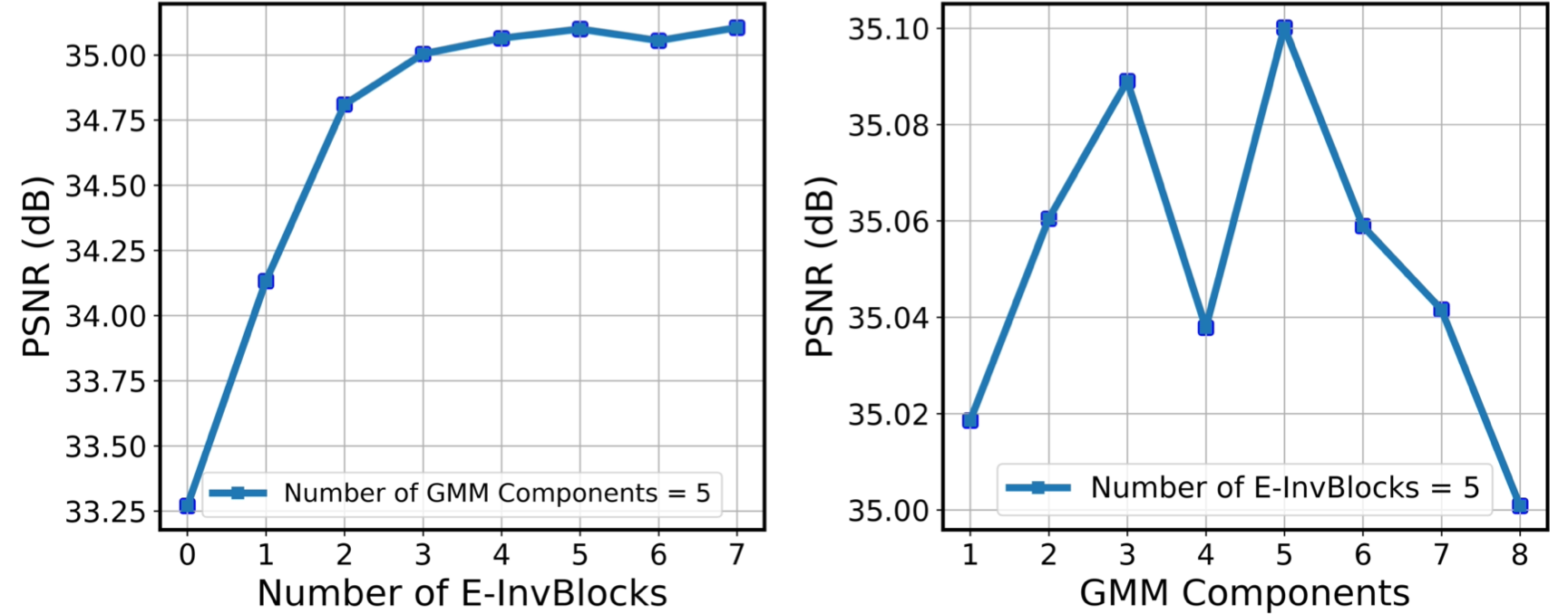
Figure 6: Effect of the number of E-InvBlocks and GMM components. Evaluated at JPEG QF=75 on DIV2K ($\times 2$).

5 Further Analysis

5.1 Hyper-Parameter Selection

We mainly investigate the influence of different settings of the hyper-parameters related to the model structure. We fixed the total number of blocks as 8 (for $\times 2$ task) and search for the best value of the number of E-InvBlocks. It actually searches for a complexity balance between the downscaling module $f$ and the compression simulator $g$. From Fig. 6, we observe that the performance saturates after this value reaches 5. Since adding E-InvBlocks would increase the number of parameters, we use 5 and 10 E-InvBlocks for $\times 2$ and $\times 4$ experiments, respectively. Besides, we can find that the best value of GMM components $K$ is 5. Too large or too small values both degrade the performance. An analysis of the effect of the training QF is in the supplementary.

5.2 Evaluation under WebP Distortion

WebP (Google 2010) is a modern compression format that is widely used for images on the Internet. Therefore, we further validate the tolerance against WebP of the proposed model. To make the optimization end-to-end, we still use the differentiable JPEG simulator as the virtual codec $\varepsilon$ to approximate the gradient but set WebP as the real compression $\epsilon$ to guide the behavior of the invertible compression simulator $g$. We test the image rescaling ($\times 2$) performance at the WebP QF of 30 and 90. Tab. 4 again shows the robustness against real compression artifacts of our model, which demonstrates the potential to extend to other image compression methods.

$\mathcal{N}(0,1)$ $\rightarrow$GMM	$\mathcal{L}_{rel}$	$\mathcal{L}_{fit}^{\prime}$	$\mathcal{L}_{reg}$	Set5	DIV2K
	✓	✓	✓	35.98	35.01
✓		✓	✓	36.02	35.02
✓	✓		✓	35.85	34.95
✓	✓	✓		35.95	34.96
✓	✓	✓	✓	36.04	35.10

Table 3: Ablation study of PSNR under JPEG QF=75.

Downscaling & Upscaling	QF	PSNR / SSIM
Bicubic & Bicubic	90	32.02 / 0.8922
Bicubic & SRCNN (Dong et al. 2015)	90	31.29 / 0.9014
Bicubic & EDSR (Lim et al. 2017)	90	34.32 / 0.9220
Bicubic & RDN (Zhang et al. 2018b)	90	34.26 / 0.9212
Bicubic & RCAN (Zhang et al. 2018a)	90	34.34 / 0.9222
CAR & EDSR (Sun and Chen 2020)	90	32.58 / 0.8918
IRN (Xiao et al. 2020)	90	33.38 / 0.9140
SAIN (Ours)	90	35.83 / 0.9410
Bicubic & Bicubic	30	29.75 / 0.8244
Bicubic & SRCNN (Dong et al. 2015)	30	28.47 / 0.8160
Bicubic & EDSR (Lim et al. 2017)	30	29.62 / 0.8249
Bicubic & RDN (Zhang et al. 2018b)	30	29.64 / 0.8252
Bicubic & RCAN (Zhang et al. 2018a)	30	29.54 / 0.8235
CAR & EDSR (Sun and Chen 2020)	30	28.03 / 0.7800
IRN (Xiao et al. 2020)	30	29.86 / 0.8303
SAIN (Ours)	30	33.15 / 0.9144

Table 4: Quantitative results on DIV2K against WebP.

6 Conclusion

Existing image rescaling models are fragile to compression artifacts. In this work, we present a novel self-asymmetric invertible network (SAIN) that is robust to lossy compression. It approximates the downscaling and compression processes in one forward pass by virtue of the proposed E-InvBlock, and thus can inversely restore the compression distortions for improved upscaling. We leverage a learnable GMM distribution to capture a generic knowledge shared across samples, and carefully design the loss functions to benefit approximations and restorations. Extensive experiments prove that our model performs far better than previous methods under the distortion of standard image codecs and is flexible to be extended to other compression formats.

Figure 7: *

Supplementary Material

Figure 8: Additional qualitative results of image rescaling ($\times 2$) on DIV2K under distortion at different JPEG QFs.

Figure 9: Qualitative results of image rescaling ($\times 4$) on DIV2K under distortion at different JPEG QFs.

Appendix A Log-Jacobian Determinant of E-InvBlock

Flow-based methods usually requires a tractable Jacobian to directly maximize the log-likelihood of the input distribution. Although we optimize our model in a different manner, the proposed E-InvBlock also allows for easy computation of the log-Jacobian determinant.

The forward step of the E-InvBlock consists of 3 steps:

$$y_{i}=x_{l}^{i}+\varphi\left(x_{h}^{i}\right)~{};\\$$ (12)

$$x_{l}^{i+1}=y_{i}-\phi\left(x_{h}^{i}\right)~{};\\$$ (13)

$$x_{h}^{i+1}=x_{h}^{i}\odot e^{\left(\rho\left(x_{l}^{i+1}\right)\right)}+\eta\left(x_{l}^{i+1}\right)~{}.$$ (14)

And the corresponding Jacobians of each step are:

$$J_{1}=\left[\begin{array}[]{ll}1&*\\ 0&1\end{array}\right];J_{2}=\left[\begin{array}[]{ll}1&*\\ 0&1\end{array}\right];J_{3}=\left[\begin{array}[]{ll}1&0\\ &e^{\left(\rho\left(x_{l}^{i+1}\right)\right)}\end{array}\right]~{},$$ (15)

where $*$ denotes the components whose exact forms are unimportant. So the overall log-Jacobian determinant is:

$$\log\left|\operatorname{det}\left(J_{1}*J_{2}*J_{3}\right)\right|$$ (16)

$$= \log\left|\operatorname{det}\left(J_{1}\right)\right|+\log\left|\operatorname{det}\left(J_{2}\right)\right|+\log\left|\operatorname{det}\left(J_{3}\right)\right|$$

$$= ~{}0+0+\rho\left(x_{l}^{i+1}\right)~{}.$$

Appendix B Visual Results under JPEG Distortion

More Image Rescaling ($\times 2$) Results

We demonstrate additional visual results of the top methods in image rescaling ($\times 2$) under JPEG distortions in Fig.8

Image Rescaling ($\times 4$) Results

Due to space limitation, the qualitative results of image rescaling ($\times 4$) are omitted in the manuscript. These results are shown in Fig. 9. Apparently, at a larger scale like $\times 4$, previous methods are even more fragile to the JPEG distortions. In contrast, our model has the ability to obtain rather high-quality reconstructions.

Downscaled LR Results

As shown in Fig. 10, the downscaled results produced by our model is similar to the results of Bicubic downscaling in visual perception.

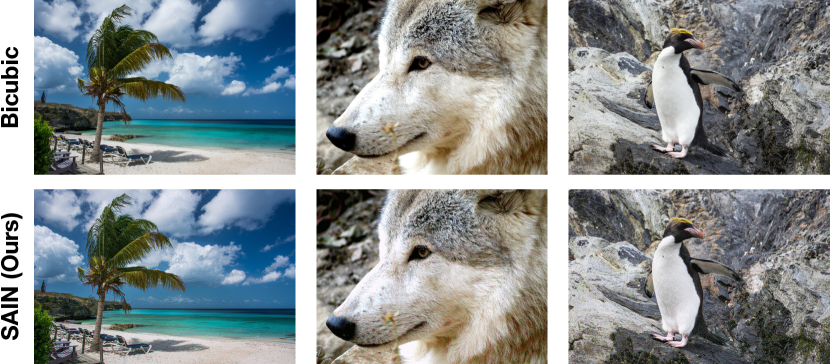
Figure 10: Visual results of downscaled images on DIV2K.

Appendix C Visual Results under WebP Distortion

Since we incorporate real image compression to guide the training objectives, our method can also be easily applied to other compression formats. Some visual demonstrations of image rescaling under WebP distortions are presented in Fig. 11. Although we leverage a differentiable JPEG implementation to surrogate the gradients of real image compression, our method still exhibits satisfactory robustness to the WebP compression.

Appendix D Effect of Training QFs

In the main experiments, we empirically train our model with the compression QF fixed at 75. As shown in Tab. 5, the model trained at QF=75 performs much better in higher QFs like 75 and 50. We hypothesize that training with too low QF such as 25 severely degrades the quality of LR image representations and thus makes distortion recovery too difficult. Given that the compression QF used in real scenarios is usually larger than 50, it is natural to focus more on the reconstruction performance at higher QFs.

Besides, in our experiments, we also find that training with mixed compression QFs is also unfavorable to improve model performance.

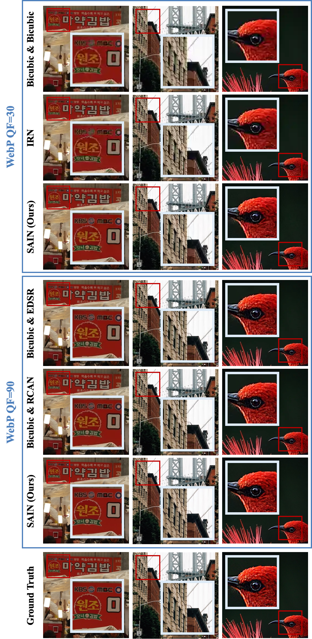
Figure 11: Qualitative results of image rescaling ($\times 2$) on DIV2K under distortion at different WebP QFs.

PSNR (dB)	(Testing QF=) 75	50	25
(Training QF=) 75	35.10	33.17	30.89
50	33.88	32.99	31.23
25	29.37	29.34	29.14

Table 5: Effect of different training QFs. The results are evaluated on DIV2K under JPEG distortion.

References

- Agustsson and Timofte (2017) Agustsson, E.; and Timofte, R. 2017. Ntire 2017 challenge on single image super-resolution: Dataset and study. In Proceedings of the IEEE conference on computer vision and pattern recognition workshops, 126–135.
- Améndola, Engström, and Haase (2020) Améndola, C.; Engström, A.; and Haase, C. 2020. Maximum number of modes of Gaussian mixtures. Information and Inference: A Journal of the IMA, 9(3): 587–600.
- Bengio, Léonard, and Courville (2013) Bengio, Y.; Léonard, N.; and Courville, A. 2013. Estimating or propagating gradients through stochastic neurons for conditional computation. arXiv preprint arXiv:1308.3432.
- Bevilacqua et al. (2012) Bevilacqua, M.; Roumy, A.; Guillemot, C.; and Alberi-Morel, M. L. 2012. Low-complexity single-image super-resolution based on nonnegative neighbor embedding. In Proceedings of the British Machine Vision Conference, 135.1–135.10.
- Dai et al. (2019) Dai, T.; Cai, J.; Zhang, Y.; Xia, S.-T.; and Zhang, L. 2019. Second-order attention network for single image super-resolution. In Proceedings of the IEEE/CVF conference on computer vision and pattern recognition, 11065–11074.
- Dinh, Krueger, and Bengio (2014) Dinh, L.; Krueger, D.; and Bengio, Y. 2014. Nice: Non-linear independent components estimation. arXiv preprint arXiv:1410.8516.
- Dinh, Sohl-Dickstein, and Bengio (2016) Dinh, L.; Sohl-Dickstein, J.; and Bengio, S. 2016. Density estimation using real nvp. arXiv preprint arXiv:1605.08803.
- Dong et al. (2015) Dong, C.; Loy, C. C.; He, K.; and Tang, X. 2015. Image super-resolution using deep convolutional networks. IEEE transactions on pattern analysis and machine intelligence, 38(2): 295–307.
- Google (2010) Google. 2010. Web Picture Format. https://chromium.googlesource.com/webm/libweb, note = Accessed: 2023-03-10.
- Guo et al. (2022) Guo, M.; Zhao, S.; Li, Y.; Li, J.; Zhang, L.; and Wang, Y. 2022. Invertible Single Image Rescaling via Steganography. In 2022 IEEE International Conference on Multimedia and Expo (ICME), 1–6. IEEE.
- Ho et al. (2019) Ho, J.; Chen, X.; Srinivas, A.; Duan, Y.; and Abbeel, P. 2019. Flow++: Improving flow-based generative models with variational dequantization and architecture design. In International Conference on Machine Learning, 2722–2730. PMLR.
- Huang, Singh, and Ahuja (2015) Huang, J.-B.; Singh, A.; and Ahuja, N. 2015. Single image super-resolution from transformed self-exemplars. In Proceedings of the IEEE conference on computer vision and pattern recognition, 5197–5206.
- Jang, Gu, and Poole (2017) Jang, E.; Gu, S.; and Poole, B. 2017. Categorical Reparameterization with Gumbel-Softmax. In International Conference on Learning Representations.
- Kim et al. (2018) Kim, H.; Choi, M.; Lim, B.; and Lee, K. M. 2018. Task-aware image downscaling. In Proceedings of the European Conference on Computer Vision (ECCV), 399–414.
- Kingma and Ba (2014) Kingma, D. P.; and Ba, J. 2014. Adam: A method for stochastic optimization. arXiv preprint arXiv:1412.6980.
- Kingma and Dhariwal (2018) Kingma, D. P.; and Dhariwal, P. 2018. Glow: Generative flow with invertible 1x1 convolutions. Advances in neural information processing systems, 31.
- Kingma and Welling (2013) Kingma, D. P.; and Welling, M. 2013. Auto-encoding variational bayes. arXiv preprint arXiv:1312.6114.
- Kobyzev, Prince, and Brubaker (2020) Kobyzev, I.; Prince, S. J.; and Brubaker, M. A. 2020. Normalizing flows: An introduction and review of current methods. IEEE transactions on pattern analysis and machine intelligence, 43(11): 3964–3979.
- Kornblith et al. (2019) Kornblith, S.; Norouzi, M.; Lee, H.; and Hinton, G. 2019. Similarity of neural network representations revisited. In International Conference on Machine Learning, 3519–3529. PMLR.
- Li et al. (2018) Li, Y.; Liu, D.; Li, H.; Li, L.; Li, Z.; and Wu, F. 2018. Learning a convolutional neural network for image compact-resolution. IEEE Transactions on Image Processing, 28(3): 1092–1107.
- Liang et al. (2021) Liang, J.; Lugmayr, A.; Zhang, K.; Danelljan, M.; Van Gool, L.; and Timofte, R. 2021. Hierarchical conditional flow: A unified framework for image super-resolution and image rescaling. In Proceedings of the IEEE/CVF International Conference on Computer Vision, 4076–4085.
- Lienhart and Maydt (2002) Lienhart, R.; and Maydt, J. 2002. An extended set of haar-like features for rapid object detection. In Proceedings. international conference on image processing, volume 1, I–I. IEEE.
- Lim et al. (2017) Lim, B.; Son, S.; Kim, H.; Nah, S.; and Mu Lee, K. 2017. Enhanced deep residual networks for single image super-resolution. In Proceedings of the IEEE conference on computer vision and pattern recognition workshops, 136–144.
- Lugmayr et al. (2020) Lugmayr, A.; Danelljan, M.; Gool, L. V.; and Timofte, R. 2020. Srflow: Learning the super-resolution space with normalizing flow. In European conference on computer vision, 715–732. Springer.
- Martin et al. (2001) Martin, D.; Fowlkes, C.; Tal, D.; and Malik, J. 2001. A database of human segmented natural images and its application to evaluating segmentation algorithms and measuring ecological statistics. In Proceedings Eighth IEEE International Conference on Computer Vision. ICCV 2001, volume 2, 416–423. IEEE.
- Rezende and Mohamed (2015) Rezende, D.; and Mohamed, S. 2015. Variational inference with normalizing flows. In International conference on machine learning, 1530–1538. PMLR.
- Son et al. (2021) Son, H.; Kim, T.; Lee, H.; and Lee, S. 2021. Enhanced standard compatible image compression framework based on auxiliary codec networks. IEEE Transactions on Image Processing, 31: 664–677.
- Sun and Chen (2020) Sun, W.; and Chen, Z. 2020. Learned image downscaling for upscaling using content adaptive resampler. IEEE Transactions on Image Processing, 29: 4027–4040.
- Wallace (1992) Wallace, G. K. 1992. The JPEG still picture compression standard. IEEE transactions on consumer electronics, 38(1): xviii–xxxiv.
- Wang et al. (2018) Wang, X.; Yu, K.; Wu, S.; Gu, J.; Liu, Y.; Dong, C.; Qiao, Y.; and Change Loy, C. 2018. Esrgan: Enhanced super-resolution generative adversarial networks. In Proceedings of the European conference on computer vision (ECCV) workshops, 0–0.
- Wang et al. (2004) Wang, Z.; Bovik, A. C.; Sheikh, H. R.; and Simoncelli, E. P. 2004. Image quality assessment: from error visibility to structural similarity. IEEE transactions on image processing, 13(4): 600–612.
- Xiao et al. (2020) Xiao, M.; Zheng, S.; Liu, C.; Wang, Y.; He, D.; Ke, G.; Bian, J.; Lin, Z.; and Liu, T.-Y. 2020. Invertible image rescaling. In European Conference on Computer Vision, 126–144. Springer.
- Xing, Qian, and Chen (2021) Xing, Y.; Qian, Z.; and Chen, Q. 2021. Invertible image signal processing. In Proceedings of the IEEE/CVF Conference on Computer Vision and Pattern Recognition, 6287–6296.
- Zeyde, Elad, and Protter (2010) Zeyde, R.; Elad, M.; and Protter, M. 2010. On single image scale-up using sparse-representations. In International conference on curves and surfaces, 711–730. Springer.
- Zhang et al. (2018a) Zhang, Y.; Li, K.; Li, K.; Wang, L.; Zhong, B.; and Fu, Y. 2018a. Image super-resolution using very deep residual channel attention networks. In Proceedings of the European conference on computer vision (ECCV), 286–301.
- Zhang et al. (2018b) Zhang, Y.; Tian, Y.; Kong, Y.; Zhong, B.; and Fu, Y. 2018b. Residual dense network for image super-resolution. In Proceedings of the IEEE conference on computer vision and pattern recognition, 2472–2481.