A Nyström method for scattering by a two-layered medium with a rough boundary

Abstract

This paper presents a study on the integral equation method and the Nystöm method for the scattering of time-harmonic acoustic waves by a two-layered medium with an unbounded perturbed boundary. The medium consists of two layers separated by a plane interface, for which we assume transmission boundary conditions. We assume either Dirichlet or impedance boundary conditions for the rough surface boundary. Unlike classical rough surface scattering problems, the presence of a plane interface makes it difficult to establish the well-posedness of the scattering problem and to find a numerical treatment. We introduce the two-layered Green function and prove that this function has similar asymptotic decay properties to the half-space Green function. By using a similar approach to classical rough surface problems, we establish the uniqueness of the scattering problem. We derive the integral equation formulations using the two-layered Green function as the integral kernel and use them to prove the existence of the scattering problem. Furthermore, we propose the Nystöm method for discretizing the integral equations and establish its convergence. Finally, we perform numerical experiments to demonstrate the effectiveness of the Nystöm method.

Keywords: the two-layered Green function, the two-layered medium, integral equation method, Nyström method.

1 Introduction

This paper focuses on the mathematical analysis of scattering problems of time-harmonic acoustic waves from a two-layered medium with a planar interface. The boundary of the two-layered medium is assumed to be a rough surface, which refers to a non-local perturbation of the planar surface whose height is within a finite distance from the original plane. Scattering problems of this type are of continuous concern in various engineering applications such as ground-penetrating radar, seismic exploration, ocean exploration, photonic crystal, and diffraction by gratings. For an introduction and historical remarks, we refer to [15, 32, 17, 29, 33, 30].

There has been already a vast literature on rough surface scattering problems for acoustic, electromagnetic and elastic waves. We refer the reader to [10, 35, 7, 6] for the integral equation methods applied to the Dirichlet or impedance boundary value problem, which uses layer potential techniques to transfer the scattering problem to equivalent boundary integral equation. The references [34, 9, 11] consider the scattering by penetrable interfaces and inhomogeneous layers. For the variational approach we refer to [4, 3] for the rough surface scattering problem with unpenetrable rough boundary in the non-weighted space and weighted space. The paper [23] extends the method in [4] to the scattering by finite height inhomogeneous layer with the Nuemann and generarized impedance boundary boundary. The papers [18, 19, 21, 26, 22] also consider the scattering by electromagnetic and elastic waves.

In addition to the well-posedness, there have been several numerical methods developed for rough surface scattering problems. Meier established the Nyström method for the unbounded integral equation in [27], which departs from the traditional Nyström method that is only suitable for the bounded integral equation. Chen and Wu come up with an adaptive finite element method with PML for the wave scattering by periodic structures in [14]. The paper [5] introduces the PML method for unbounded rough surface scattering problem and establishes the linear convergence. Recently, the paper [37] proves that exponential convergence holds locally for the scattering problem with periodic surfaces. Lastly, we note that if the rough surface is periodic and is exposed to quasi-periodic incident waves, the scattering problem can be solved by using the quasi-periodic Green function. The [36] provides a competitive algorithm for computing the quasi-periodic Green function based on FFT, which is particularly efficient when a large number of values are required.

The objective of this paper is to establish the well-posedness of the scattering problem with Dirichlet and impedance boundary conditions using the integral equation method and to propose a corresponding numerical method. Since we assume transmission boundary conditions on the planar interface of the two-layered medium, it is natural to use the two-layered Green function, which overcomes the difficulties caused by the presence of the planar interface. We prove that the two-layered Green function has similar asymptotic decay properties to the half-space Dirichlet Green function and the half-space impedance Green function using the methods outlined in [25].

We follow the framework of proofs of the well-posedness of classical rough surface scattering problem for the bounded continuous boundary data as presented in [9, 35]. To prove the uniqueness of Dirichlet and impedance boundary problems, we use the two-layered Green function to construct a Green integral representation to the scattered field with respect to the homogeneous boudnary condition. We then show the density function in the integral repersentaition vanishes. To establish the existence of the scattering problem, we construct boundary integral equations that are equivalent to the scattering problem apply integral equation theory for the real line as estabilshed by [8] to prove the well-posedness of the solutions to integral equations.

To obtain numerical solutions, we establish Nyström methods based on the integral equation used to prove the existence of the scattering problem. Firstly, we discretize the integral equations. The two-layered Green function is the sum of the free space Green function and the perturbation term. We write the integral equation in the form of the Nyström method, as described in [27]. Using the asymptotic decay property and the convergence theory in [27], we prove the convergence of the numerical solution with an error estimate with respect to the smoothness. The numerical results show that the Nyström methods give good approximations to the scattered field for virtual point source incidence and plane wave incidence.

The remaining sections of the paper are organized as follows. Section 2 introduces the scattering problems and their corresponding boundary problems. In Section 3, we focus on introducing the properties of the two-layered Green function, with the proof of the asymptotic property given there. Section 4 demonstrates the well-posedness of the boundary value problems, which includes a prior estimate of the scattered field, the uniqueness results, and the proof of existence. Section 5 constructs the Nyström method of the integral equations, providing a proof of convergence and numerical experiments. Appendix A provides the potential theory, while Appendix B offers integral operator theory on the real line.

2 Mathematical models of the scattering problems

In this section, we introduce the mathematical models of the scattering problems. To this end, we give some notations, which will be used throughout the paper. Let $V\subset\mathbb{R}^{n}$ ($n=1,2$), we denotes by $BC(V)$ the set of functions bounded and continuously on $V$, a Banach space under the norm $\|\phi\|_{\infty,V}:=\sup_{x\in V}|\phi(x)|$. For $0<\alpha\leq 1$, we denote by $C^{0,\alpha}(V)$ the Banach space of functions $\phi\in BC(V)$, which are uniformly Hölder continuously with exponent $\alpha$ and with norm $\|\cdot\|_{C^{0,\alpha}(V)}$ defined by $\|\phi\|_{C^{0,\alpha}(V)}:=\|\phi\|_{\infty,V}+\sup_{x,y\in V,x\neq y}[|\phi(x)-\phi(y)|/|x-y|^{\alpha}]$. We let $C^{1,\alpha}(\mathbb{R}):=\{\phi\in BC(\mathbb{R})\cap C^{1}(\mathbb{R}):\phi^{\prime}\in C^{0,\alpha}(\mathbb{R})\}$, a Banach space under the norm $\|\phi\|_{C^{1,\alpha}(\mathbb{R})}:=\|\phi\|_{\infty,\mathbb{R}}+\|\phi^{\prime}\|_{C^{0,\alpha}(\mathbb{R})}$. For any $a\in\mathbb{R}$, define $\Gamma_{a}:=\{(x,a):x_{1}\in\mathbb{R}\}$ and $U_{a}:=\left\{(x_{1},x_{2}):x_{1}\in\mathbb{R},x_{2}>a\right\}$.

Let $U_{0}$ and $\mathbb{R}\backslash\overline{U_{0}}$ denote the medium in lower and upper half-spaces, respectively. The interface of the two-layered medium is denoted by $\Gamma_{0}$. The wave number of the medium in lower and upper half-spaces are $k_{+}$ and $k_{-}$ respectively. Assume $k_{+}\neq k_{-}$, which means the medium in the sides of $\Gamma_{0}$ are different. There is a rough surface $\Gamma$ in the upper half-space $\mathbb{R}^{2}\backslash\overline{U_{0}}$ (see Figure 2.1). Consider $f\in C^{1,1}(\Gamma)$ with $f_{+}:=\sup_{x\in\mathbb{R}}f(x)<0$. Then the rough surface $\Gamma$ is defined by $\Gamma:=\left\{(x_{1},x_{2}):x_{2}=f(x_{1}),x_{1}\in\mathbb{R}\right\}$, and we further define $D:=\{(x_{1},x_{2}):x_{2}>f(x_{1})\}$, $f_{-}:=\inf_{x\in\mathbb{R}}f(x)$, and $L:=\|f^{\prime}\|_{\infty,\mathbb{R}}$ which will be used later.

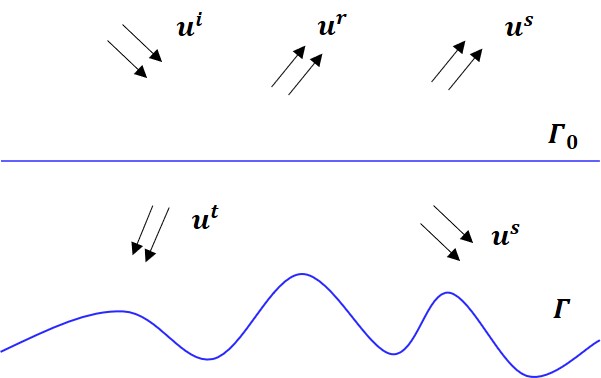
Figure 2.1: Geometry

Consider the scattering problems with time-harmonic incident waves in the domain $D$. The incident wave $u^{i}$ will produce the reference wave $u^{0}$. Then the total field $u=u^{0}+u^{s}$ is the sum of the reference wave and the scattered wave $u^{s}$, satisfies the following Helmholtz equation on both side of the interface $\Gamma_{0}$

$$\left\{\begin{aligned} &\Delta u+k_{+}^{2}u=0&&\text{ in }U_{0},\\ &\Delta u+k_{-}^{2}u=0&&\text{ in }D\backslash\overline{U_{0}}.\end{aligned}\right.$$

Moreover, we assume the total field $u$ satisfies the following boundary conditions on the interface $\Gamma_{0}$.

$$u_{+}=u_{-},\left.\frac{\partial u}{\partial x_{2}}\right|_{+}=\left.\frac{\partial u}{\partial x_{2}}\right|_{-}\text{ on }\Gamma_{0}.$$

Further, the boundary condition need to be imposed on $\Gamma$ which depends on the physical property of the rough surface. We restricts our attention to the following two cases:

(1) The case when the total field vanishes on the boundary, i.e, the total field $u$ the Dirichlet boundary condition $u=0\text{ on }\Gamma$.

(2) The case when the total field satisfies the homogeneous impedance boundary condition $\partial u/\partial\nu-\textrm{i}k_{2}\beta u=0\text{ on }\Gamma$, here $\beta\in BC(\Gamma)$, $\nu(x)$ denotes the unit normal at $x\in\Gamma$ pointing out of $D$ and $\partial u/\partial\nu$ denotes the normal derivative of $u$.

To ensure the uniqueness of the scattering problem, the scattered field $u^{s}$ is required to satisfies a radiation condition. Different from the bounded obstacle scattering problem, here we need to require $u^{s}$ to satisfy so-called upward propagating radiation conditon in $U_{0}$, that is, for some $h>0$, and $\phi\in L^{\infty}(\Gamma_{h})$, there holds

$$u^{s}(x)=2\int_{\Gamma_{h}}\frac{\partial\Phi_{k_{+}}(x,y)}{\partial y_{2}}\phi(y)ds(y),x\in U_{h},$$ (2.1)

where $\Phi_{k_{+}}(x,y):=\frac{i}{4}H_{0}^{1}(k_{+}|x-y|)$, $x,y\in\mathbb{R}^{2}$, with $x\neq y$ is the free-space Green function for Helmholtz equation with wave number $k_{+}$.

Now we describe the reference wave $u^{0}$ more specificly. The reference wave is the total field of the scattering problem in the two-layered medium without the rough surface. The reference wave $u^{0}$ satisfies the following conditions

$$\left\{\begin{aligned} &\Delta u^{0}+k_{+}u^{0}=0&&\text{ in }U_{0},\\ &\Delta u^{0}+k_{-}u^{0}=0&&\text{ in }\mathbb{R}^{2}\backslash\overline{U_{0}},\\ &u^{0}_{+}=u^{0}_{-},\left.\frac{\partial u^{0}}{\partial x_{2}}\right|_{+}=\left.\frac{\partial u^{0}}{\partial x_{2}}\right|_{-}&&\text{ on }\Gamma_{0}.\end{aligned}\right.$$

In this paper, we consider two types of the incident waves: plane wave and point-source wave. Suppose the plane wave $u^{i}(x):=e^{ik_{+}x\cdot d}$ is the incident wave, here $d:=(\cos(\theta_{d}),\sin(\theta_{d})),\theta_{d}\in[0,2\pi)$, $\theta_{d}\in[\pi,2\pi]$. Then the reference wave $u^{0}$ is given by (see, e.g., (2.13a) and (2.13b) in [28] or Section 4 in [25])

$$u^{0}(x)=\left\{\begin{array}[]{ll}u^{i}(x)+u^{r}(x),&\text{ in }U_{0},\\ u^{t}(x),&\text{ in }\mathbb{R}^{2}\backslash\overline{U_{0}},\end{array}\right.$$ (2.2)

with

$$u^{r}(x):=\mathcal{R}(\pi+\theta_{d})e^{ik_{+}x\cdot d^{r}},\quad u^{t}(x):=\mathcal{T}(\pi+\theta_{d})e^{ik_{-}x\cdot d^{t}},$$

where $d^{r}=(\cos(\theta_{d}),-\sin(\theta_{d}))$ is the reflected direction, $d^{t}=n^{-1}(\cos(\theta_{d}^{t}),-\mathrm{i}\mathcal{S}(\cos\theta_{d},n))$. Particularly, if $|n^{-1}\cos(\theta_{d})|\leq 1$, then $d^{t}$ is the transmitted direction with $\theta_{d}^{t}\in[\pi,2\pi]$ satisfying $\cos(\theta_{d}^{t})=n^{-1}\cos(\theta_{d})$. $\mathcal{R}\left(\pi+\theta_{d}\right)$ and $\mathcal{T}\left(\pi+\theta_{d}\right)$ are called reflected coefficient and transmitted coefficient, respectively, with $\mathcal{R}$ and $\mathcal{T}$ are defined by

$$\mathcal{R}(\theta):=\frac{\mathrm{i}\sin\theta+\mathcal{S}(\cos\theta,n)}{\mathrm{i}\sin\theta-\mathcal{S}(\cos\theta,n)},\quad\mathcal{T}(\theta):=\mathcal{R}(\theta)+1\quad\text{ for }\theta\in\mathbb{R},$$

where $S(z,a)$ is a function for $z\in\mathbb{R}$ and $a>0$ defined by

$$\mathcal{S}(z,a):=\left\{\begin{array}[]{ll}-\mathrm{i}\sqrt{a^{2}-z^{2}}&\text{ if }a^{-1}|z|\leq 1,\\ \sqrt{z^{2}-a^{2}}&\text{ if }a^{-1}|z|>1.\end{array}\right.$$ (2.3)

The range of $z$ in $\mathcal{S}$ can be extended to the complex plane. The specific definition of $S$ in the complex plane will be given in Section 3.

Suppose the incident wave is the point source wave propagated at $y$ with $y\in U_{0}$, then $u^{i}$ is given by $u^{i}(x):=\Phi_{k_{+}}(x,y)$ for $y\in U_{0}$. Here, $\Phi_{k_{+}}(x,y):=\frac{\mathrm{i}}{4}H_{0}^{1}(k_{+}|x-y|)$. Then, the reference wave $u^{0}(x)=G(x,y)$, where $G(x,y)$ denotes so-called the two-layered Green function.

For $x\in\mathbb{R}^{2}$, and $y\in\mathbb{R}^{2}\backslash\Gamma_{0}$, the two-layered Green function $G(x,y)$ is the solution of the following scattering problem (see page 17 in [28])

$$\Delta_{x}G(x,y)+k^{2}G(x,y) =-\delta(x-y) \text{ in }\mathbb{R}^{2}\backslash\Gamma_{0},$$

$$G(x,y)|_{+}=G(x,y)|_{-},\partial_{x_{2}}G(x,y)|_{+} =\partial_{x_{2}}G(x,y)|_{-} \text{ on }\Gamma_{0},$$

$$\lim\limits_{|x|\to\infty}\left(\frac{\partial G(x,y)}{\partial|x|}-\mathrm{i}kG(x,y)\right) =0, \text{ uniformly for all }\frac{x}{|x|}\in U_{0}\text{ and }\frac{x}{|x|}\in\mathbb{R}^{2}\backslash\overline{U}_{0},$$ (2.4)

where $k:=k_{+}$ in $U_{0}$ and $k:=k_{-}$ in $\mathbb{R}^{2}\backslash\overline{U}_{0}$, $\delta$ denotes the Dirac delta distribution, (2.4) is called the Sommerfeld radiation condition.

Now the above scattering problems can be formulated as the following two boundary value problems (DBVP) and (IBVP) for the scattered field $u^{s}$.

Definition 2.1 ($\mathscr{R}^{D}(D)$).

Let $\mathscr{R}^{D}(D)$ denotes the set of function $v\in C^{2}(D\backslash\Gamma_{0})\cap C(\overline{D})$, $v|_{\overline{U}_{0}}\in C^{1}(\overline{U}_{0})$ and $v|_{D\backslash U_{0}}\in C^{1}(D\backslash U_{0})$.

Dirichlet Boundary Value Problem (DBVP) Given $g\in BC(\Gamma)$, determine $u^{s}\in\mathscr{R}^{D}(D)$ such that:

(i) $u^{s}$ is a solution of the Helmholtz equation

$$\begin{cases}\Delta u^{s}+k_{+}u^{s}=0\text{ in }U_{0},\\ \Delta u^{s}+k_{-}u^{s}=0\text{ in }\mathbb{R}\backslash\overline{U_{0}};\end{cases}$$

(ii) $u^{s}_{+}=u^{s}_{-}$, $\left.\partial_{x_{2}}u^{s}\right|_{+}=\left.\partial_{x_{2}}u^{s}\right|_{-}\text{ on }\Gamma_{0}$;

(iii) $u=g$ on $\Gamma$;

(iv) For some $\alpha\in\mathbb{R}$

$$\sup_{x\in D}|(x_{2}+|f_{-}|+1)^{\alpha}u^{s}(x)|<\infty;$$ (2.5)

(v) $u^{s}$ satisfies the upward propagating radiation condition (2.1) in $\mathbb{U}_{0}$ with wave number $k_{+}$.

Definition 2.2 ($\mathscr{R}^{I}(D)$).

Let $\mathscr{R}^{I}(D)$ denote the set of functions $v\in C^{2}(D\backslash\Gamma_{0})\cap C(\overline{D})$ satisfies $v|_{\overline{U}_{0}}\in C^{1}(\overline{U}_{0})$, and $v|_{D\backslash U_{0}}\in C^{1}(D\backslash U_{0})$ for which the normal derivative of $v$ defined by $\partial v/\partial\nu(x):=\lim_{h\to 0+}\nu(x)\cdot\Delta(x-h\nu(x))$, with the convergence uniformly in $x$ on every compact subset of $\Gamma$.

Impedance Boundary Value Problem (IBVP) Given $g\in BC(\Gamma),\beta\in BC(\Gamma)$, determine $u\in\mathscr{R}^{I}(D)$, such that:

(i) $u^{s}$ is a solution of the Helmholtz equation

$$\begin{cases}\Delta u^{s}+k_{+}u^{s}=0\text{ in }U_{0},\\ \Delta u^{s}+k_{-}u^{s}=0\text{ in }\mathbb{R}\backslash\overline{U_{0}};\end{cases}$$

(ii) $u^{s}_{+}=u^{s}_{-},\partial u^{s}/\partial x_{2}\left|{}_{+}=\partial u^{s}/\partial x_{2}\right|_{-}$ on $\Gamma_{0}$;

(iii) $\partial u^{s}/\partial\nu-\mathrm{i}k_{-}\beta u^{s}=g$ on $\Gamma$;

(iv) $u^{s}$ satisfies (2.5) for some $a\in\mathbb{R}$;

(v) For some $\theta\in(0,1)$ and some constant $C_{\theta}>0$, there holds

$$\left|\nabla u(x)\right|\leq C_{\theta}[x_{2}-f(x_{1})]^{\theta-1}$$

for $x\in D_{b}$, where $b=f_{+}/2$;

(vi) $u^{s}$ satisfies the upward propagating radiation condition (2.1) in $U_{0}$ with wave number $k_{+}$.

Remark 2.3.

The boundedness condition (2.5) and the condition (v) in the problem (IBVP) are required in the uniqueness proof of the problems (DBVP) and (IBVP).

Remark 2.4.

Plane-wave incidence Suppose that $u^{s}$ is the scattered field of plane-wave incidence with the incident direction $d$ as defined in Section 2, then $u^{s}$ satisfies the problem (DBVP) with $g(x)=-u^{0}(x)=-u^{t}(x)$. Suppose that $u^{s}$ is the scattered field of plane wave incidence, then $u^{s}$ satisfies the problem (IBVP) with $g(x)=-\partial u^{t}(x)/\partial\nu+\mathrm{i}k_{-}\beta u^{t}(x)$. Here we see that $u^{t}\in BC(\Gamma)$, which means the assumptions $g\in BC(\Gamma)$ in the definition of the problems (DBVP) and (IBVP) are resonable.

Point-source incidence Suppose that $u^{s}$ is the scattered field of point-source incidence, then for any source point $y\in D\backslash\Gamma_{0}$, $u^{s}$ satisfies the problem (DBVP) with $g(x)=-G(x,y)$. Suppose that $u^{s}$ is the scattered field of point-source incidence, then $u^{s}$ satisfies the problem (IBVP) with $g(x)=-\partial G(x,y)/\partial\nu+\mathrm{i}k_{-}\beta G(x,y)$.

3 Properties of the two-layered Green function

In order to prove the well-posedness of boundary value problems and the convergence of the Nystr"om methods, we need to introduce some properties of the two-layered Green function.

$G(x,y)$ has the expression (see the reference [28])

$$G(x,y)=\begin{cases}\Phi_{k_{+}}(x,y)+\frac{1}{4\pi}\int_{-\infty}^{\infty}\frac{\mathcal{S}\left(\xi,k_{+}\right)-\mathcal{S}\left(\xi,k_{-}\right)}{\mathcal{S}\left(\xi,k_{+}\right)+\mathcal{S}\left(\xi,k_{-}\right)}\frac{e^{-\mathcal{S}\left(\xi,k_{+}\right)\left|x_{2}+y_{2}\right|}}{\mathcal{S}\left(\xi,k_{+}\right)}e^{\mathrm{i}\xi\left(x_{1}-y_{1}\right)}d\xi,x_{2}\geq 0,y_{2}\geq 0,\\ \frac{1}{2\pi}\int_{-\infty}^{\infty}\frac{e^{\mathcal{S}\left(\xi,k_{-}\right)y_{2}-\mathcal{S}\left(\xi,k_{+}\right)x_{2}}}{\mathcal{S}\left(\xi,k_{+}\right)+\mathcal{S}\left(\xi,k_{-}\right)}e^{\mathrm{i}\xi\left(x_{1}-y_{1}\right)}d\xi,x_{2}\geq 0,y_{2}\leq 0,\\ \frac{1}{2\pi}\int_{-\infty}^{\infty}\frac{e^{-\mathcal{S}\left(\xi,k_{+}\right)y_{2}+\mathcal{S}\left(\xi,k_{-}\right)x_{2}}}{\mathcal{S}\left(\xi,k_{+}\right)+\mathcal{S}\left(\xi,k_{-}\right)}e^{\mathrm{i}\xi\left(x_{1}-y_{1}\right)}d\xi,x_{2}\leq 0,y_{2}\geq 0,\\ \Phi_{k_{-}}(x,y)+\frac{1}{4\pi}\int_{-\infty}^{\infty}\frac{\mathcal{S}\left(\xi,k_{-}\right)-\mathcal{S}\left(\xi,k_{+}\right)}{\mathcal{S}\left(\xi,k_{+}\right)+\mathcal{S}\left(\xi,k_{-}\right)}\frac{e^{-\mathcal{S}(\xi,k-)\left|x_{2}+y_{2}\right|}}{\mathcal{S}\left(\xi,k_{-}\right)}e^{\mathrm{i}\xi\left(x_{1}-y_{1}\right)}d\xi,x_{2},y_{2}\leq 0,\end{cases}$$ (3.1)

where $\Phi_{k_{-}}(x,y):=\frac{\mathrm{i}}{4}H_{0}^{1}(k_{-}|x-y|),x,y\in\mathbb{R}^{2},x\neq y$ is the free-space Green function for Helmholtz equation with wave number $k_{-}$. Further, it is seen from (3.1) that

$$G(x,y)=\frac{\mathrm{i}}{4}H_{0}^{1}(k_{-}|x-y|)+R(x,y)\text{ for }x,y\in\mathbb{R}^{2}\backslash\overline{U}_{0},$$ (3.2)

here $R(x,y)\in C^{\infty}(\mathbb{R}^{2}\backslash\overline{U}_{0},\mathbb{R}^{2}\backslash\overline{U}_{0})$.

From the (3.1), it is seen that $G(x,y)$ has the following symmetry property (see also page 20 of [28])

$$G(x,y)=G(y,x),x\neq y.$$ (3.3)

It is important for this paper that the $G(x,y)$ has the following asymptotic property.

Theorem 3.1.

For $k_{+},k_{-},B>0$ with $k_{+}\neq k_{-}$, let $x=(x_{1},x_{2})$ and $y=(y_{1},y_{2})$, assume $x_{2}>-B$ and $y_{2}>-B$, then $G(x,y)$ and $\nabla_{y}G(x,y)$ satisfy the following estimates

$$\left|G(x,y)\right|,\left|\nabla_{y}G(x,y)\right|\leq C\frac{1+|x_{2}|+|y_{2}|}{|x-y|^{\frac{3}{2}}+|x-y^{\prime}|^{\frac{3}{2}}},\text{ for }|x-y|>1,$$ (3.4)

where the constant $C$ depends only on $k_{+}$, $k_{-}$ and $B$.

Similar properties are founded in the half-plane Dirichlet Green function and the half-plane impedance Green function (see [35, inequalites (8) and (24)]).

The remaining part of this section is devoted to proving Theorem 3.1, using the approach presented in [25]. Our proof follows the following outline: first, we represent the integral in (3.1) as integrals over specific curves, as described in [25]. We apply a similar analysis to [25] to obtain the asymptotic properties of each part. Finally, by combining the results from Lemmas 3.2-3.4, we obtain the proof of Theorem 3.1.

Using the following integral representation of Hankel function (see [15, formula (2.2.11)]),

$$\frac{\mathrm{i}}{4}H_{0}^{1}(k|x-y|)=\frac{1}{4\pi}\int_{-\infty}^{+\infty}\frac{e^{-\mathcal{S}(\xi,k)|x_{2}-y_{2}|}}{\mathcal{S}(\xi,k)}e^{\mathrm{i}\xi(x_{1}-y_{1})}d\xi,$$

the formula (3.1) of $G(x,y)$ can be written as

$$G(x,y)=\begin{cases}G_{D}(x,y,k_{+})+G_{R_{1}}(x,y),x_{2}\geq 0,y_{2}\geq 0,\\ G_{R_{2}}(x,y),x_{2}\geq 0,y_{2}\leq 0,\\ G_{R_{3}}(x,y),x_{2}\leq 0,y_{2}\geq 0,\\ G_{D}(x,y,k_{-})+G_{R_{4}}(x,y),x_{2}\leq 0,y_{2}\leq 0,\end{cases}$$ (3.5)

where

$$G_{D}(x,y,k_{+}):=\frac{\mathrm{i}}{4}H_{0}^{1}(k_{+}|x-y|)-\frac{\mathrm{i}}{4}H_{0}^{1}(k_{+}|x-y|)$$

$$G_{D}(x,y,k_{-}):=\frac{\mathrm{i}}{4}H_{0}^{1}(k_{-}|x-y|)-\frac{\mathrm{i}}{4}H_{0}^{1}(k_{-}|x-y|)$$

$$G_{R_{1}}(x,y):=\frac{1}{2\pi}\int_{-\infty}^{+\infty}\frac{1}{\mathcal{S}(\xi,k_{+})+\mathcal{S}(\xi,k_{1})}e^{-\mathcal{S}(\xi,k_{+})(x_{2}+y_{2})}e^{\mathrm{i}\xi(x_{1}-y_{1})}d\xi$$ (3.6)

$$G_{R_{4}}(x,y):=\frac{1}{2\pi}\int_{-\infty}^{+\infty}\frac{1}{\mathcal{S}(\xi,k_{+})+\mathcal{S}(\xi,k_{1})}e^{\mathcal{S}(\xi,k_{+})(x_{2}+y_{2})}e^{\mathrm{i}\xi(x_{1}-y_{1})}d\xi$$

and $G_{R_{2}}(x,y)$, $G_{R_{3}}(x,y)$ are defined as in formula (3.1).

Let $n:=k_{-}/k_{+}$, define the angle $\theta_{c}:=$ by

$$\theta_{c}:=\left\{\begin{array}[]{lr}\mathrm{arccos}(n),&k_{+}>k_{-},\\ \mathrm{arccos}(1/n),&k_{+}<k_{-}.\end{array}\right.$$

Now we give the definition of $\mathcal{S}(z,a)$ for $z\in\mathbb{D}$ and $a>0$. Firstly, let $\mathbb{C}_{1}$ and $\mathbb{C}_{2}$ defined by

$$\mathbb{C}_{1}:=\mathbb{C}\backslash\{z\in\mathbb{C}:\operatorname{Im}(z)\geq 0,\operatorname{Re}(z)=0\},$$

$$\mathbb{C}_{2}:=\mathbb{C}\backslash\{z\in\mathbb{C}:\operatorname{Im}(z)\leq 0,\operatorname{Re}(z)=0\}.$$

Then, we introduce the function $\mathcal{S}_{1}$ and $\mathcal{S}_{2}$ as follows:

(i) For $z\in\mathbb{C}_{1}$ with $z=|z|e^{\mathrm{i}\theta_{1}}$ and $\theta_{1}\in(-\frac{3\pi}{2},\frac{\pi}{2})$, let $\mathcal{S}_{1}(z):=\sqrt{|z|}e^{\mathrm{i}\theta_{1}/2}$. For $z=0$ define $\mathcal{S}_{1}(z):=0$.

(ii) For $z\in\mathbb{C}_{2}$ with $z=|z|e^{\mathrm{i}\theta_{2}}$ and $\theta_{2}\in(-\frac{\pi}{2},\frac{3\pi}{2})$, let $\mathcal{S}_{2}(z):=\sqrt{|z|}e^{\mathrm{i}\theta_{2}/2}$. For $z=0$ define $\mathcal{S}_{2}(z):=0$.

For $z\in\mathbb{C}$ and $a>0$ such that $z-a\in\mathbb{C}_{1}\cup\{0\}$ and $z+a\in\mathbb{C}_{2}\cup\{0\}$, define $\mathcal{S}(z,a):=\mathcal{S}_{1}(z-a)\mathcal{S}_{2}(z+a)$. It is seen that the definition here of $\mathcal{S}$ is an extention of $S$ defined by (2.3). Let $\mathcal{D}$ and $\mathcal{L}_{o}$ be defined as in [25]. The the following lemmas hold.

Lemma 3.2.

Assume that $k_{+}>k_{-}$. Let $x-y^{\prime}=r^{\prime}(\cos(\theta),\sin(\theta))$ with $\theta\in(0,\pi/2)$ and $r^{\prime}=|x-y^{\prime}|$. Then the following statements (a) and (b) hold.

(a) For $\theta\in[\theta_{c},\pi/2)$, we have

$$G_{R_{1}}(x,y)=G_{R_{1}}^{(1)}(x,y)+G^{(2)}_{R_{1}}(x,y)$$

where $G_{R_{1}}^{(1)}$ and $G^{(2)}_{R_{1}}$ are given by

$$G_{R_{1}}^{(1)}(x,y) :=\frac{-\textrm{i}}{2\pi}\int_{\mathcal{D}}\frac{\sin^{2}(\zeta)}{n^{2}-1}e^{\textrm{i}k_{+}r^{\prime}\cos(\zeta-\theta)}d\zeta,$$ (3.7)

$$G_{R_{1}}^{(2)}(x,y) :=\frac{1}{2\pi}\int_{\mathcal{D}}\frac{\sin\zeta S(\cos\zeta,n)}{n^{2}-1}e^{\textrm{i}k_{+}r^{\prime}cos(\zeta-\theta)}d\zeta.$$

(b) For $\theta\in(0,\theta_{c})$, we have

$$G_{R_{1}}(x,y)=G_{R_{1}}^{(1)}(x,y)+G_{R_{1}}^{(3)}(x,y)+G_{R_{1}}^{(4)}(x,y),$$

where $G_{R_{1}}^{(1)}$ is given by (3.7), and $G_{R_{1}}^{(3)}$ and $G_{R_{1}}^{(3)}$ are given by

$$G_{R_{1}}^{(3)}(x,y) :=\frac{1}{2\pi}\int_{\mathcal{D}}\frac{\sin\zeta S(\cos\zeta,n)}{n^{2}-1}e^{\textrm{i}k_{+}r^{\prime}cos(\zeta-\theta)}d\zeta,$$

$$G_{R_{1}}^{(4)}(x,y) :=\frac{1}{2\pi}\int_{\mathcal{L}_{o}}\frac{\sin\zeta S(\cos\zeta,n)}{n^{2}-1}e^{\textrm{i}k_{+}r^{\prime}cos(\zeta-\theta)}d\zeta.$$

Proof.

When $x_{2},y_{2}>0$, $G_{R_{1}}(x,y)$ has the expression (3.6). Take the variable substitution $\xi=\cos(z),z\in L$, where $L$ is the path $+\infty\mathrm{i}\to 0\to\pi\to\pi-\infty\mathrm{i}$ in the complex plane $\mathbb{C}$. Then

$$G_{R_{1}}(x,y) =\frac{1}{2\pi}\int_{L}\frac{1}{-\mathrm{i}\sin(z)+\mathcal{S}(\cos(z),n)}e^{\mathrm{i}k_{+}|x-y^{\prime}|\cos(z-\theta)}(-1)\sin(z)dz,$$

$$=\frac{1}{2\pi}\int_{L}\frac{-\textrm{i}\sin^{2}(z)+\sin(z)S(\cos(z),n)}{n^{2}-1}e^{\mathrm{i}k_{+}|x-y^{\prime}|\cos(z-\theta)}dz.$$

By setting $y=(0,0)$ and replacing $x$ with $x-y^{\prime}$ in [25, Lemma 2.4], we can see that $G_{\mathcal{R}}^{(j)}(x-y^{\prime},0)$ in [25, Lemma 2.4] has the same value as $G_{R_{1}}^{j}(x,y)$ for $j=2,3,4$. The only difference between Lemma 3.2 and [25, Lemma 2.4] is the expression (3.7) for $G_{R_{1}}^{(1)}(x,y)$, which can also be derived in a similar way as in [25, Lemma 2.4]. ∎

Lemma 3.3.

Assume that $k_{+}>k_{-}$. Suppose that $x-y^{\prime}=r^{\prime}(\cos\theta,\sin\theta)$ with $r^{\prime}=|x-y^{\prime}|$ and $\theta\in[\theta_{c},\pi-\theta_{c}]$, then we have tha asymptotic behaviors

$$G_{R_{1}}^{(1)}(x,y)=-\frac{e^{\textrm{i}k_{+}r^{\prime}}}{\sqrt{r^{\prime}}}\frac{\textrm{i}\sin\theta(1+\cos\theta)}{2\sqrt{\pi}(n^{2}-1)k_{+}}+G_{R_{1},Res}^{(1)}(x,y)$$ (3.8)

and

$$G^{(2)}_{R_{1}}(x,y)=\frac{e^{\textrm{i}k_{+}r^{\prime}}}{\sqrt{r^{\prime}}}\frac{e^{\textrm{i}\frac{\pi}{4}}}{\sqrt{8\pi k_{+}}}\frac{2\textrm{i}\sin\theta S(\cos\theta,n)}{n^{2}-1}+G_{R_{1},Res}^{(2)}(x,y).$$ (3.9)

where $G^{(1)}_{R_{1},Res}(x,y)$ and $G^{(2)}_{R_{1},Res}(x,y)$ satisfy

$$\left|G^{(1)}_{R_{2},Res}(x,y)\right|\leq Cr^{\prime-\frac{3}{2}}, r^{\prime}\to+\infty$$ (3.10)

$$\left|G^{(2)}_{R_{2},Res}(x,y)\right|\leq Cr^{\prime-\frac{3}{4}}, r^{\prime}\to+\infty$$ (3.11)

uniformly for all $\theta\in[\theta_{c},\pi-\theta_{c}]$ and

$$\left|G_{R_{2},Res}^{(2)}(x,y)\right|\leq C\left|\theta_{c}-\theta\right|^{-\frac{3}{2}}r^{\prime-\frac{3}{2}},r^{\prime}\to+\infty,$$ (3.12)

uniformly for all $\theta\in[\theta_{c},\pi-\theta_{c}]$. Here, the constant $C$ is independent of $x$ and $y$.

Proof.

Since Lemma 3.2 is similar to [25, Lemma 2.4], the only term we need to analyze is $G^{(1)}_{R_{1},Res}$. To do that, we follow Step 2 in the proof of Lemma 2.10 in [25]. Firstly, we rewrite $G^{(1)}_{R_{1}}(x,y)$ by

$$G^{(1)}_{R_{1}}(x,y)=\frac{\textrm{i}e^{\textrm{i}k_{+}|x|}}{4\pi}\int_{-\infty}^{+\infty}g_{1}(s)e^{-|x|s^{2}}ds,$$

where

$$g_{1}(s):=\frac{\sin^{2}(\zeta)}{n^{2}-1}\frac{d\zeta(s)}{ds},$$

and $\zeta(s)$ is a bijective from $\mathbb{R}$ to $\mathcal{D}$ defined by $\zeta(s):=2\arcsin(Q(s))+\theta$, and $Q(s)$ is given by $Q(s):=se^{-\mathrm{i}\pi/4}/\sqrt{2k_{+}}$. By Taylor’s expansion of $g_{1}(s)$, we obtain that

$$G^{(1)}_{R_{1}}(x,y) =\frac{\textrm{i}e^{\textrm{i}k_{+}|x|}}{4\pi}\left(\int_{-\infty}^{+\infty}g_{1}(0)e^{-|x|s^{2}}ds+\int_{-\infty}^{+\infty}g^{\prime}_{1}(0)se^{-|x|s^{2}}ds+\frac{\textrm{i}e^{\textrm{i}k_{+}|x|}}{4\pi}G_{R_{1},Res}^{(1)}(x,y)\right)$$

$$=-\frac{e^{\textrm{i}k_{+}r^{\prime}}}{\sqrt{r^{\prime}}}\frac{\textrm{i}\sin\theta(1+\cos\theta)}{2\sqrt{\pi}(n^{2}-1)k_{+}}+G_{R_{1},Res}^{(1)}(x,y)$$ (3.13)

where $G^{(1)}_{R_{1},Res}(x,y):=\int_{-\infty}^{+\infty}g_{1,Res}(s)e^{-|x|s^{2}}ds$ with $g_{1,Res}(s):=g_{1}(s)-g_{1}(0)-g^{\prime}_{1}(0)s$. Analogous to the derivation of (2.46) in [25], we deduce that $|g_{2}(s)|\leq C(1+|s|^{3})e^{C|s|^{2}}$ for any $s\in L_{\tilde{\sigma}}$, where the definition of $L_{\tilde{\sigma}}$ is the same as in [25]. Then it follows from Cauchy inequality (see [31, Corollary 4.3]) that

$$\left|\frac{d^{2}g_{1}}{ds^{2}}(s)\right|\leq C(1+|s|)^{3}e^{C|s|^{2}}\textrm{ for }s\in\mathbb{R}$$

Hence, similar with the discussion in Part I of Step 1 in the proof of Lemma 2.10 in [25, Lemma 2.4], we apply the mean-value theorem for $\textrm{Re}(g_{2,Res})$ and $\textrm{Im}(g_{2,Res})$ to obtain that

$$\left|\frac{g_{1,Res}(s)}{s^{2}}\right|\leq C(1+|s|)^{3}e^{C|s|^{2}}\textrm{ for }s\in\mathbb{R}$$

Then it follows that

$$\left|G_{R_{1},Res}^{(1)}(x,y)\right| \leq C_{1}\int_{-\infty}^{+\infty}(s^{2}+s^{5})e^{-(r^{\prime}-C)s^{2}}ds$$

$$\leq C_{1}\left[(r^{\prime}-C)^{-\frac{3}{2}}+(r^{\prime}-C)^{-3}\right]\leq C_{2}r^{\prime-\frac{3}{2}}$$

holds for $r^{\prime}$ large enough. This, together with the formula (3.13), implies that $G_{R_{1}}$ has the form (3.8) and $G_{R_{1},Res}^{(1)}$ satisfies (3.10) uniformly for all $\theta\in[\theta_{c},\pi-\theta_{c}]\backslash\{\pi/2\}$. For $\theta=\pi/2$, since the direction is fixed, by using a similar arguments as in Theorem 2.1 in [25], we can obtain that $G_{R_{1},Res}(x,y)$ also satisfies (3.10) for all $\theta=\pi/2$. ∎

Lemma 3.4.

Assume that $k_{+}>k_{-}$. Suppose that $x-y^{\prime}=r^{\prime}(\cos\theta,\sin\theta)$ with $r^{\prime}=|x-y^{\prime}|$ and $\theta\in(0,\theta_{c})\cup(\pi-\theta_{c},\pi)$, then we have tha asymptotic behaviors

(a) $G_{R_{1}}^{(1)}(x,y)$ has the asymptotic behavior (2.37) with $G^{(1)}_{R_{1},Res}(x,y)$ satisfying (2.39) uniformly for all $\theta\in(0,\theta_{c})$.

(b) $G^{(3)}_{R}$(x,y) has the asymptotic behavior

$$G_{R_{1}}^{(3)}(x,y)=\frac{e^{\mathrm{i}k_{+}r^{\prime}}}{\sqrt{r^{\prime}}}\frac{e^{\mathrm{i}\frac{\pi}{4}}}{\sqrt{8\pi k_{+}}}\frac{2\mathrm{i}\sin\theta S\left(\cos\theta,n\right)}{n^{2}-1}+G_{R_{1},Res}^{(3)}(x,y)$$

with $G_{R_{1},Res}^{(3)}(x,y)$ satisfying

$$\left|G_{R_{1},Res}^{(3)}(x,y)\right| \leq Cr^{\prime-\frac{3}{4}}, r^{\prime}\to+\infty,$$ (3.14)

$$\left|G_{R_{1},Res}^{(3)}(x,y)\right| \leq C\left|\theta_{c}-\theta\right|^{-\frac{3}{2}}r^{\prime-\frac{3}{2}}, r^{\prime}\to+\infty,$$ (3.15)

uniformly for all $\theta\in(0,\theta_{c})\cup(\pi-\theta_{c},\pi)$.

(c) $G_{R_{1}}^{(4)}(x,y)$ satisfies

$$\left|G_{R_{1}}^{(4)}(x,y)\right| \leq Cr^{\prime-\frac{3}{4}}, r\to+\infty,$$ (3.16)

$$\left|G_{R_{1},Res}^{(4)}(x,y)\right| \leq C|\theta_{c}-\theta|^{-\frac{3}{2}}r^{\prime-\frac{3}{2}} r\to+\infty,$$ (3.17)

uniformly for all $\theta\in(0,\theta_{c})\cup(\pi-\theta_{c},\pi)$.

Here, the constant $C$ is independent of $x$ and $y$.

Now we are ready to give the proof of Theorem 3.1.

Proof of Theorem 3.1 we only consider the case $k_{+}>k_{-}$, the analysis in the case $k_{+}<k_{-}$ is similar. We consider the following cases (a)-(d) respectively.

(a) Suppose $x_{2}=y_{2}=0$, we use the analysis in [28, P38-39, (2.56b)] and get

$$G(x,y)\sim\frac{\textrm{i}\sqrt{n}}{\sqrt{2\pi}\left(1-n^{2}\right)}\frac{\mathrm{e}^{ik_{-}\left|x_{1}-y_{1}\right|+\mathrm{i}\pi/4}}{\left(k_{+}\left|x_{1}-y_{1}\right|\right)^{3/2}}-\frac{\textrm{i}}{\sqrt{2\pi}\left(n^{2}-1\right)}\frac{\mathrm{e}^{ik_{+}\left|x_{1}-y_{1}\right|+\mathrm{i}\pi/4}}{\left(k_{+}\left|x_{1}-y_{1}\right|\right)^{3/2}},$$

as $|x_{1}-y_{1}|\to\infty$, then

$$\left|G(x,y)\right|\leq C\frac{1}{|x_{1}-y_{1}|^{\frac{3}{2}}}$$

as $|x-y|>1$.

Suppose the $x_{2}$ and $y_{2}$ are both not equal to $0$, we consider the following the cases (b) $x_{2},y_{2}\geq 0$, (c) $x_{2}\geq 0,y_{2}\leq 0$ (d) $x_{2}\leq 0,y_{2}\geq 0$ and (e) $x_{2}\leq 0,y_{2}\leq 0$.

(b) Suppose $x_{2},y_{2}\geq 0$, let $x-y^{\prime}=(x_{1}-y_{1},x_{2}+y_{2})=r^{\prime}(\cos(\theta),\sin(\theta))$ with $r^{\prime}=|x-y^{\prime}|$ and $\theta_{c}\in(0,\pi)$. We recall that $G(x,y)=G_{D}(x,y)+G_{R_{1}}(x,y)$. Here $G_{D}$ satisfies the estimate (see the formula $(8)$ in the reference [35])

$$|G(x,y)|,\left|\nabla_{y}G(x,y)\right|\leqslant C\left(1+\left|x_{2}\right|\right)\left(1+\left|y_{2}\right|\right)\left\{|x-y|^{-3/2}+\left|x-y^{\prime}\right|^{-3/2}\right\}.$$

Hence we only need to estimate the remained term $G_{R_{1}}(x,y)$. In view of the Lemma 3.2, Lemma 3.3 and Lemma 3.4, we see, if $\theta\in[\theta_{c},\pi-\theta_{c}]$, then from the formula (3.8, 3.9), we need to estimate the main term and remain term of $G_{R_{1}}^{(1)}$ and $G_{R_{1}}^{(2)}$ and if $\theta\in(0,\theta_{c})\cup(\pi-\theta_{c},\pi)$, we need to estimate the main term and the remain term of $G_{R_{1}}^{(1)}(x,y)$, $G_{R_{1}}^{(3)}(x,y)$ and $G_{R}^{(4)}(x,y)$. Note that $\sin(\theta)=(x_{2}+y_{2})/r^{\prime}$, therefore the norm of the main term of $G_{R_{1}}^{(1)}$, $G_{R_{1}}^{(2)}$, $G_{R_{1}}^{(3)}$, $G_{R_{1}}^{(4)}$ are all less than the right hand side of the formula (3.4).

To estimate the remain term, we need to divide the interval $[0,\pi]$ into two parts.

(i) $\theta\in[\theta_{c}/2,\pi-\theta_{c}/2]$, in this case there holds $|x_{1}-y_{1}|\leq\tan(\theta_{c}/2)(x_{2}+y_{2})$, then from the formula (3.11,3.14, 3.16),

$$|G_{R_{1},Res}^{(2)}(x,y),|G_{R_{1},Res}^{(3)}(x,y)|,|G_{R_{1},Res}^{(3)}(x,y)|\leq Cr^{\prime-\frac{3}{4}}\leq C(x_{2}+y_{2})/r^{\prime\frac{3}{2}}.$$

this together with the formula (3.10), i.e.

$$\left|G_{R_{1},Res}^{(1)}(x,y)\right|\leq r^{\prime-\frac{3}{2}},$$

we obtain that $|G(x,y)|$ is less than the right hand side of (3.4).

(ii) $(0,\theta_{c}/2]\cup[\pi-\theta_{c}/2,\pi)$ then from the formula (3.12, 3.15, 3.17),

$$|G_{R_{1},Res}^{(2)}(x,y),|G_{R_{1},Res}^{(3)}(x,y)|,|G_{R_{1},Res}^{(3)}(x,y)|\leq C|\theta_{c}/2|r^{\prime\frac{3}{2}}.$$

this together with the formula (3.10), i.e.

$$\left|G_{R_{1},Res}^{(1)}(x,y)\right|\leq r^{\prime-\frac{3}{2}},$$

we obtain that $|G(x,y)|$ is less than the right hand side of (3.4).

(c) Suppose $x_{2}\geq 0,y_{2}\leq 0$. By making a variable substitution $\xi=k_{+}\zeta$ we can write $G_{R_{2}}$ in the following form

$$G_{R_{2}}(x,y)=\frac{1}{2\pi}\int_{-\infty}^{+\infty}\frac{e^{k_{+}(S(\zeta,n)-S(\zeta,1))y_{2}}}{S(\zeta,1)+S(\zeta,n)}e^{\textrm{i}k_{+}[\zeta(x_{1}-y_{1})-S(\zeta,1)(x_{2}-y_{2})]}d\zeta.$$

We use this form, and follow the approach of estimate of $G_{\tau}(x,y)$ in [25]. Note that the term $k_{+}(S(\zeta,n)-S(\zeta,1))y_{2}$ does not contain $y_{1}$, then the requirement of $y$ in some ball in [25] can be changed to $|y_{2}|<B$, and the constant $C$ in right hand side of (3.4) depends on $B$.

(d) & (e) In the case of (d) $x_{2}\leq 0,y_{2}\geq 0$ and (e) $x_{2}\leq 0,y_{2}\leq 0$. We use the the symmetry of the two-layered Green fuction in the formula (3.3), i.e.,

$$G(x,y)=G(y,x),x\neq y.$$

This reduces the proofs of (d) and (e) to the proofs of (b) and (c), which completes the proof.

4 The well-posedbess of the boundary value problems

In this section, we focus on the uniqueness of the solution of the problems (DBVP) and (IBVP). Firstly, we give some a piror estimates in subsection 4.1, and then following the approach in the reference [35], we gives the uniqueness proof of the problem (DBVP) in subsection 4.2. The uniqueness proof of (IBVP) is given in subsection 4.3. The existence results of the problem (DBVP) and (IBVP) are given in subsection 4.4 and subsection 4.5, respectively.

4.1 The derivative estimate

Now we show some estimates of the first derivative of solution which will be used in the uniqueness proofs. Suppose $u^{s}\in\mathscr{R}^{D}(D)$ satisfies conditions (i)-(iv) of the problem (DBVP) (with $g\equiv 0$). Then by standard ellipic regularity estimate [20, Thm 8.34], $u^{s}\in C^{1}(\overline{D})$. We also need the boundedness estimate of derivative of scattered fields. Let $L_{\infty}(G)$ denote the essentially bounded function defined on $G$. Then the following lemma can be proved by the gradient estimate of Poisson’s equation (see [9, Lemma 2.7] and the references given there).

Lemma 4.1 (Lemma 2.7, [9]).

If $G\subset\mathbb{R}^{2}$ is open and bounded, $v\in L_{\infty}(G)$, and $\Delta v=f\in L_{\infty}(G)$ (in a distributional sense) then $v\in C^{1}(G)$ and

$$|\nabla v(x)|\leqslant C(d(x))^{-1}\left(\|v\|_{\infty}+\left\|d^{2}f\right\|_{\infty}\right),\quad x\in G,$$

where $C$ is an absolute constant and $d(x)=\operatorname{dist}(x,\partial G)$.

Use Lemma 4.1, we can obtain the estimate of $\nabla u^{s}$ in $D$. In fact, for $x=(x_{1},x_{2})\in D$, take a ball $B$ centered at $x$. Then by using Lemma 4.1 in $B$ for $u^{s}$, together with the formula (2.5), the following Theorem 4.2 holds.

Theorem 4.2.

If $u^{s}\in\mathscr{R}^{D}(D)$ satisfies conditions (i)-(iv) of the problem (DBVP) (with $g\equiv 0$), or $u^{s}\in\mathscr{R}^{I}(D)$ satisfies conditions (i)-(iv) of the problem (IBVP) (with $g\equiv 0$), then there exists some $\alpha\in\mathbb{R}$ such that

$$\sup_{x\in D^{\epsilon}}(|x_{2}|+1)^{\alpha}|\nabla u^{s}(x)|<\infty$$

for all $\epsilon\in(0,|f_{+}|)$, where $D^{\epsilon}=\left\{x=(x_{1},x_{2})|x_{1}\in\mathbb{R},x_{2}>f(x_{1})+\epsilon\right\}$.

The parameter $\epsilon$ in the Theorem 4.2 is chosen since our method do not allow us to get the estimate near the boundary of $D$. In fact, following the proof in [10, Theorem 3.1] which uses the maximum principle of Poisson’s equation in the region of polygon, we can obtain the following estimate of $u^{s}$ and $\nabla u^{s}$ for the problem (DBVP).

Theorem 4.3.

If $u^{s}\in\mathscr{R}^{D}(D)$ satisfies condition (i)-(iii) of the problem (DBVP) with $g\equiv 0$, then for some positive constant C,

(i) $|u^{s}(x)|\leq C[x_{2}-f(x_{1})]^{\alpha}$

(ii) $|\nabla u^{s}(x)|\leq C[x_{2}-f(x_{1})]^{\alpha-1}$

hold for $x\in\{x|x_{1}\in\mathbb{R},f(x_{1})<x_{2}<f(x_{1})+\epsilon\}$ , where $\epsilon:=\frac{|f_{+}|}{2}$ and $\frac{1}{2}<\alpha<\frac{\pi}{(2\pi-\theta)}<1$, $\theta:=\pi-2\arctan(L)$.

Proof.

The theorem here is strongly similar to [10, Theorem 3.1]. The difference between Theorem 4.3 and [10, Theorem 3.1] is the appearance of the interface $\Gamma_{0}$. In fact, in order to give the proof of Theorem 4.3, we only need to make a simple modification of the proof of [10, Theorem 3.1]. We change the definition of $E$ and $\eta(x)$ in the proof the [10, Theorem 3.1] to be $E:=2|f_{+}|/3$ and $\eta:=\min(|f_{+}|/6,d(x))$ respectively. Here, here $|f_{+}|/6$ is chosen so that for $x\in D\backslash\overline{U}_{f_{+}/2}$, the ball centered at $x$ and of radius $|f_{+}|/6$ is contained in $D\backslash U_{f_{+}/3}$. ∎

4.2 The uniqueness reuslt of the problem (DBVP)

With the help of the a piror estimates in subsection 4.1, now we can derive the uniqueness proof of the problem (DBVP). Firstly we use a Rellich’s type identity to obtain the upper bound of $L^{2}$ integral of the normal derivative of $u^{s}$ on $\Gamma$. For this purpose, we define some notations. For $B,A\in\mathbb{R}$ with $B<A$, define $\Gamma_{0}(B,A):=\{(x_{1},0):B<x_{1}<A\}$ and $\Gamma(B,A):=\{(x_{1},x_{2}):B<x_{1}<A,x_{2}=f(x_{1})\}$. For $t\in\mathbb{R}$, define $\gamma(t):=\left\{\left.(x_{1},x_{2})\right|f(x_{1})<x_{2}<0,x_{1}=t\right\}$.

Theorem 4.4.

Assume $k_{+}>k_{-}$. Let $u^{s}\in\mathscr{R}^{D}(D)$ be the solution of the problem (DBVP) with $g=0$ and define $T(B,A):=\left\{x\in D\backslash\overline{U}_{0}:B<x_{1}<A\right\}$. Then we have

$$\int_{\Gamma(B,A)}\left|\frac{\partial u^{s}}{\partial\nu}\right|^{2}ds\leq C\left[I_{1}(B,A)+R_{1}(B,A)\right],$$ (4.1)

where $\nu=(\nu_{1},\nu_{2})$ denotes the outward unit normal to $\partial T(B,A)$, and $I_{1}(B,A)$ and $R_{1}(B,A)$ are given by

$$I_{1}(B,A):= \int_{\Gamma_{0}(B,A)}\left[|\partial_{2}u_{+}^{s}|^{2}-|\partial_{1}u_{+}^{s}|^{2}+k_{+}^{2}|u_{+}^{s}|^{2}\right]ds,$$

$$R_{1}(B,A):= \,2\textrm{Re}\left[\int_{\gamma(A)}-\int_{\gamma(B)}\right]\partial_{2}\overline{u^{s}}\partial_{1}u^{s}ds.$$

Here, $C$ is a constant depending only on $\Gamma$.

Proof.

Note that Rellich’s type identity $2\textrm{Re}[\overline{\partial_{2}u^{s}}(\Delta u^{s}+k_{-}^{2}u^{s})]=2\textrm{Re}[\nabla(\overline{\partial_{2}u^{s}}\nabla u^{s})]-\partial_{2}(|\nabla u^{s}|^{2})+k_{-}^{2}\partial_{2}(|u^{s}|^{2})$ holds on $D$. Thus apply the divergence theorem in $T(A,B)$, we obtain

$$0=\int_{\partial T(A,B)}\left[2\textrm{Re}(\partial_{2}\overline{u^{s}}\nabla u^{s})\cdot\nu-|\nabla u^{s}|^{2}\nu_{2}+k_{-}^{2}|u^{s}|^{2}\nu_{2}\right]ds=I_{1}+I_{2}+I_{3},$$

where $I_{1}$, $I_{2}$ and $I_{3}$ are given by

$$I_{1}: =\int_{\Gamma_{0}(B,A)}\left[|\partial_{2}u_{-}^{s}|^{2}-|\partial_{1}u_{-}^{s}|^{2}+k_{-}^{2}|u_{-}^{s}|^{2}\right]ds,$$

$$I_{2}: =2\textrm{Re}\left[\int_{\gamma(A)}-\int_{\gamma(B)}\right]\partial_{2}\overline{u^{s}}\partial_{1}u^{s}ds,$$

$$I_{3}: =\int_{\Gamma(B,A)}\left[2\textrm{Re}(\partial_{2}\overline{u^{s}}\nabla u^{s})\cdot\nu-|\nabla u^{s}|^{2}\nu_{2}+k_{-}^{2}|u^{s}|^{2}\nu_{2}\right]ds.$$

It follows from Theorems 4.2 and 4.3 that the integral $I_{2}$ is well-defined and thus we have

$$\sup_{t\in\mathbb{R}}\left|2\textrm{Re}\int_{\gamma(t)}\partial_{2}\overline{u^{s}}\partial_{1}u^{s}ds\right|<\infty.$$ (4.2)

Since $\nabla u^{s}(x)=\partial_{\nu}u^{s}\cdot{\nu}(x)$ on $\Gamma$ due to the boundary condition of $u^{s}$, we obtain $|\nabla u^{s}|^{2}=|\partial_{\nu}u^{s}|^{2}$ and $\partial_{2}u^{s}(x)=\partial_{\nu}u^{s}\nu_{2}$ on $\Gamma$. This implies that

$$I_{3}=\int_{\Gamma(B,A)}|\partial_{\nu}u^{s}|^{2}\nu_{2}ds.$$

Note further that $\nu_{2}=-1/\sqrt{1+|f^{\prime}|^{2}}\leq-1/\sqrt{1+L^{2}}$. Therefore, from the above discussions, the transmission boundary condition of $u^{s}$ on $\Gamma_{0}$ and the assumptions $k_{+}>k_{-}$, it follows that

$$\int_{\Gamma(B,A)}|\partial_{\nu}u_{-}^{s}|^{2}ds \leq\sqrt{L^{2}+1}\left(\int_{\Gamma_{0}(B,A)}(|\partial_{2}u_{-}^{s}|^{2}-|\partial_{1}u_{-}^{s}|^{2}+k_{-}^{2}|u_{-}^{s}|^{2})ds+R_{1}(B,A)\right)$$

$$\leq C\left(\int_{\Gamma_{0}(B,A)}\left(|\partial_{2}u_{+}^{s}|^{2}-|\partial_{1}u_{+}^{s}|^{2}+k_{+}^{2}|u_{+}^{s}|^{2}\right)ds+R_{1}(B,A)\right),$$

where $C$ is a constant depending only on $\Gamma$. This completes the proof. ∎

Remark 4.5.

Take $A=j,B=j-1$ and from Theorems 4.2 and Theorem 4.3, formulas (2.5) and (4.2), it follows that $\partial_{n}u\in L_{loc}^{2}(\Gamma)$, and

$$\sup_{j\in\mathbb{Z}}\int_{\Gamma(j-1,j)}|\partial_{\nu}u^{s}|^{2}ds<\infty.$$ (4.3)

In fact, the solution of the problem (DBVP) with $g=0$ can be written as the intgeral of $\partial_{\nu}u^{s}$ on $\Gamma$. And hence, to get the uniqueness result we only need to prove $\partial_{\nu}u^{s}=0$ on $\Gamma$ by the inequality (4.1). To this purpose, we define $\Gamma(A):=\left\{x:x\in\Gamma,|x_{1}|<A\right\}=\Gamma(-A,A)$ for $A>0$.

Theorem 4.6.

Let $u^{s}\in\mathscr{R}^{D}(D)$ be the solution of the problem (DBVP) with $g=0$. Then

$$u^{s}(x)=\int_{\Gamma}\partial_{\nu}u^{s}(y)G(x,y)\,ds(y),\quad x\in D\backslash U_{0},$$ (4.4)

where $\nu$ denotes the unit normal on $\Gamma$ directed to the exterior of $D$.

Proof.

Let $x=(x_{1},x_{2})\in D\backslash\overline{U}_{0}$. Define the domain

$$T_{A}^{\epsilon}:=\{x:|x_{1}|<A\}\cap D\backslash(\overline{U}_{0}\cup\overline{B_{\epsilon}(x)}),$$

where $B_{\epsilon}(x)$ denotes the ball centered at $x$ with radius $\epsilon$ small enough s.t. $\overline{B_{\epsilon}}\subset D$. Since $u^{s}\in C^{1}(\overline{D}\backslash U_{|f_{+}|/2})$ , it follows from Green theorem that

$$0 =\int_{\partial T_{A}^{\epsilon}}\left[u^{s}(y)\frac{\partial G(x,y)}{\partial\nu(y)}-\frac{\partial u^{s}}{\partial\nu}G(x,y)\right]ds(y)$$

$$=\left[\int_{S_{\epsilon}(x)}+\int_{\gamma(-A)}+\int_{\gamma(A)}+\int_{\Gamma_{0}(A)}+\int_{\Gamma(A)}\right]\left[u^{s}(y)\frac{\partial G(x,y)}{\partial\nu(y)}-\frac{\partial u^{s}}{\partial\nu}G(x,y)\right]ds(y)$$

$$=:I_{1}+I_{2}+I_{3}+I_{4}+I_{5},$$

where $\nu$ denotes the exterior unit normal on $\partial T_{A}^{\epsilon}$.

By the mean value theorem and the formula (3.1), we obtain that

$$\lim_{\epsilon\to 0+}I_{1}=\lim_{\epsilon\to 0+}\int_{\partial B_{\epsilon}(x)}\left[u^{s}(y)\frac{\partial G(x,y)}{\partial\nu(y)}-\frac{\partial u^{s}}{\partial\nu}(y)G(x,y)\right]ds(y)=u^{s}(x).$$

By the formula (3.4), Theorems 4.2 and 4.3, it follows that

$$\lim_{A\to\infty}(I_{2}+I_{3})=\lim_{A\to\infty}\left[\int_{\gamma(-A)}+\int_{\gamma(-A)}\right]\left[u^{s}(y)\frac{\partial G(x,y)}{\partial\nu(y)}-\frac{\partial u^{s}}{\partial\nu}(y)G(x,y)\right]ds(y)=0.$$

Using the transmission boundary condition on the interface $\Gamma_{0}(A)$ for $u^{s}(x)$ and $G(x,y)$, we obtain

$$I_{4} =\int_{\Gamma_{0}(A)}\left[u^{s}_{-}(y)\frac{\partial G_{-}(x,y)}{\partial y_{2}}-\frac{\partial u^{s}_{-}}{\partial y_{2}}(y)G_{-}(x,y)\right]ds(y)$$

$$=\int_{\Gamma_{0}(A)}\left[u^{s}_{+}(y)\frac{\partial G_{+}(x,y)}{\partial y_{2}}-\frac{\partial u^{s}_{+}}{\partial y_{2}}(y)G_{+}(x,y)\right]ds(y).$$

Due to formula (3.4) and Theorem 4.2, we can apply Green theorem in the domain $\left\{x:|x_{1}|<A,0<x_{2}<d\right\}$ with $d>0$ and let $A\to+\infty$ to obtain that

$$\lim_{A\to\infty}\int_{\Gamma_{0}(A)}\left[u^{s}_{+}(y)\frac{\partial G_{+}(x,y)}{\partial y_{2}}-\frac{\partial u^{s}_{+}}{\partial y_{2}}(y)G_{+}(x,y)\right]ds(y)$$

$$=\int_{\Gamma_{d}}\left[u^{s}(y)\frac{\partial G(x,y)}{\partial y_{2}}-\frac{\partial u^{s}}{\partial y_{2}}(y)G(x,y)\right]ds(y).$$

From the definition of the two-layered Green function and the formulas (3.3) and (3.4), we have $G(x,.)$ is a radiating solution in $U_{0}$, and $G(x,.)|_{\Gamma_{d}},\partial_{y_{2}}G(x,.)|_{\Gamma_{d}}\in L^{1}(\Gamma_{d})$. Note that $u^{s}$ satisfies the upward propagating radiation condition (2.1) in $U_{0}$. Hence we can employ [10, Lemma 2.1] to obtain

$$\lim_{A\to\infty}I_{4}=\int_{\Gamma_{d}}\left[u^{s}(y)\frac{\partial G(x,y)}{\partial\nu(y)}-\frac{\partial u^{s}}{\partial\nu}(y)G(x,y)\right]ds(y)=0.$$

From $u^{s}=0$ on $\Gamma$, $u^{s}\in C^{1}(\overline{D}\backslash U_{|f_{+}|/2})$, noting that $u\in L^{2}_{loc}(\Gamma)$ and formula (3.4), it follows that

$$\lim_{A\to\infty}I_{5}=-\lim_{A\to\infty}\int_{\Gamma(A)}\frac{\partial u^{s}}{\partial\nu}G(x,y)ds(y)=-\int_{\Gamma}\frac{\partial u^{s}}{\partial\nu}G(x,y)ds(y).$$

Now ultilize the above analyses, first let $\epsilon\to 0$ and then let $A\to\infty$, formula (4.4) is holds for $x\in D\backslash\overline{U}_{0}$. By the dominated convergence theorem, the formula (4.4) is also holds for $x\in\Gamma_{0}$. ∎

In order to estimate the right hand side of the inequality (4.1), we need the following two lemmas. The first one can be found in the reference [10, Lemma A].

Lemma 4.7.

Suppose that $F\in L^{2}_{\text{loc }}(\mathbb{R})$ and that, for some nonnegative constants $M$, $C$, $\epsilon$, and $A_{0}$,

$$\int_{j-1}^{j}\left|F(t)\right|^{2}dt\leq M^{2},\quad j\in\mathbb{Z}$$

and

$$\int_{-A}^{A}|F(t)|^{2}dt\leq C\int_{\mathbb{R}\backslash[-A,A]}G_{A}^{2}(t)dt+C\int_{-A}^{A}\left[G_{\infty}(t)-G_{A}(t)\right]G_{\infty}(t)dt+\epsilon,\quad A>A_{0},$$

where, for $0<A\leq+\infty$,

$$G_{A}(s):=\int_{-A}^{A}(1+|s-t|)^{-3/2}|F(t)|dt,\quad s\in\mathbb{R}.$$

Then $F\in L_{2}(\mathbb{R})$ and

$$\int_{-\infty}^{+\infty}|F(t)|^{2}dt\leq\epsilon.$$

Lemma 4.8.

Suppose $v$ satisfies one of the following two assumptions:

Assumutions (i)

$$v(x)=\int_{\Gamma(A)}\partial_{\nu}u^{s}(y)G(x,y)ds(y),\quad x\in D,$$

where $u^{s}(y)$ is a solution of the problem (DBVP) with $g=0$.

Assumptions (ii)

$$v(x)=-\int_{\Gamma(A)}\left[\frac{G(x,y)}{\partial\nu(y)}-\mathrm{i}k_{+}\beta(y)G(x,y)\right]u^{s}(y)ds(y),\quad x\in D,$$

where $u^{s}$ is a solution of the problem (IBVP) with $g=0$.

Then $v$ satisfies

$$\int_{\Gamma_{0}}\left[\left|\partial_{2}v\right|^{2}-\left|\partial_{1}v\right|^{2}+k_{+}^{2}|v|^{2}\right]ds \leq 2k_{+}\textrm{Im}\int_{\Gamma_{0}}\bar{v}\partial_{2}vds,$$

$$\textrm{Im}\int_{\Gamma_{0}}\overline{v}\partial_{2}vds \geq 0.$$

Proof.

In both assumptions (i) and (ii), there holds $v|_{\Gamma_{0}}\in BC(\Gamma_{0})\cap L^{2}(\Gamma_{0})$, $v$ satisfies Helmholtz equation and the formula (2.5), it follows from [13] that

$$v(x)=2\int_{\Gamma_{0}}\frac{\partial\Phi_{k_{+}}(x,y)}{\partial y_{2}}v(y)ds(y),\quad x\in U_{0},$$

then by [9, Lemma 6.1], for all $h>0$, there holds

$$\int_{\Gamma_{h}}\left[\left|\partial_{2}v\right|^{2}-\left|\partial_{1}v\right|^{2}+k_{+}^{2}|v|^{2}\right]ds \leq 2k_{+}\textrm{Im}\int_{\Gamma_{h}}\bar{v}\partial_{2}vds,$$

$$\mathrm{Im}\int_{\Gamma_{h}}\overline{v}\partial_{2}vds \geq 0.$$

According to the formulas (3.4) and (4.3), we obtain $v|_{\Gamma_{h}}\to v|_{\Gamma_{0}}$ $\partial_{1}v|_{\Gamma_{h}}\to\partial_{1}v|_{\Gamma_{0}}$, $\partial_{2}v|_{\Gamma_{h}}\to\partial_{2}v|_{\Gamma_{0}}$ in $L^{2}$ sense as $h\to 0$. Then let $h\to 0$ in the above inequalites, we will get the desired inequalities.

Let assumption (ii) holds, according to the formulas (2.5) and (4.3), we also obtain $v|_{\Gamma_{h}}\to v|_{\Gamma_{0}}$ $\partial_{1}v|_{\Gamma_{h}}\to\partial_{1}v|_{\Gamma_{0}}$, $\partial_{2}v|_{\Gamma_{h}}\to\partial_{2}v|_{\Gamma_{0}}$ in $L^{2}$ sense as $h\to 0$, then let $h\to 0$ in the above inequalities, we will also get the desired inequalities. ∎

We are now in a position to show $\partial_{\nu}u^{s}$ is vanishes on $\Gamma$.

For $A>0$, set $B=-A$ in formula (4.1), yieds that

$$K_{A}:=\int_{\Gamma(A)}|\partial_{n}u^{s}|^{2}ds\leq C\left[I_{1}(A)+R_{1}(A)\right],$$

where $I_{1}(A):=I(-A,A)$, $R_{1}(A):=R_{1}(-A,A)$.

In order to use Lemma 4.7, define $v$ to be the cutdown of $u$.

$$v(x):=\int_{\Gamma(A)}G(x,y)\partial_{n}u^{s}(y)ds(y)$$ (4.5)

for $x\in D\backslash\overline{U_{0}}$, then by formula (3.4) and estimate of $\partial_{n}u^{s}|_{\Gamma}$ (4.3), we have $v|_{\Gamma_{b}}$ is in $L^{2}(\Gamma_{b})\cap BC(\Gamma_{b})$ for all $0<b<|f_{+}|$. On the other hand $v$ is a radiating solution in $U_{b}$ for $b>0$, hence in the view of the equivalence of (ii) and (iv) in [10, Lemma 2.1], for each $h>0$ with $\phi=v|_{\Gamma_{h}}$. Therefore, by Lemma 4.8, $I^{\prime\prime}(A)\leq 2k_{+}J^{\prime\prime}(A)$, where

$$I^{\prime\prime}(A):=\int_{\Gamma_{a}}\left[|\partial_{2}v|^{2}-|\partial_{1}v|^{2}+k_{+}^{2}|v|^{2}\right]ds,\quad J^{\prime\prime}(A):=\textrm{Im}\int_{\Gamma_{a}}\overline{v}\partial_{2}vds.$$

Using Green theorem in domain $T:=\left\{x:x\in D\backslash\overline{U}_{0},|x_{1}|<A\right\}$, we obtain $J(A)=I_{2}(A)$, where

$$J(A):=\textrm{Im}\int_{\Gamma_{0}}\overline{u}^{s}\partial_{2}u^{s}ds,\quad R_{2}(A):=\textrm{Im}\left[\int_{\gamma_{A}}-\int_{\gamma_{-A}}\right]\overline{u}^{s}\partial_{1}u^{s}ds.$$

Whence,

$$K_{A}\leq C\left\{I_{1}(A)-I_{1}^{\prime\prime}(A)+2k_{+}\left[J^{\prime\prime}(A)-J(A)\right]+R_{1}(A)+2k_{+}R_{2}(A)\right\}.$$

In order to use Theorem 4.7, set

$$I^{\prime\prime}(A):=\int_{\Gamma_{0}(A)}\left[|\partial_{2}v|^{2}-|\partial_{1}v|^{2}+k_{+}^{2}|v|^{2}\right]ds,\quad J^{\prime\prime}(A):=\textrm{Im}\int_{\Gamma_{0}(A)}\overline{v}\partial_{2}vds.$$

Set $w\left(x_{1}\right)=\partial_{\nu}u^{s}\left(\left(x_{1},f\left(x_{1}\right)\right)\right),x_{1}\in\mathbf{R}$, then for all $A>0$,

$$\int_{-A}^{A}\left|w\left(x_{1}\right)\right|^{2}dx_{1}\leq\int_{\Gamma(A)}|\partial_{\nu}u^{s}|^{2}ds\leq\left(1+L^{2}\right)^{1/2}\int_{-A}^{A}\left|w\left(x_{1}\right)\right|^{2}dx_{1}.$$

By formulas (4.4)(4.5) and (3.4)

$$|v(x)|,|\nabla v(x)| \leq C_{a}\left(1+L^{2}\right)^{1/2}W_{A}\left(x_{1}\right),\quad x\in\Gamma_{a},$$

$$|u^{s}(x)-v(x)|,|\nabla u^{s}(x)-\nabla v(x)| \leq C_{a}\left(1+L^{2}\right)^{1/2}\left(W_{\infty}\left(x_{1}\right)-W_{A}\left(x_{1}\right)\right),\quad x\in\Gamma_{a},$$

where, for $0\leq A\leq+\infty$,

$$W_{A}\left(x_{1}\right):=\int_{-A}^{A}\left(1+\left|x_{1}-y_{1}\right|\right)^{-3/2}\left|w\left(y_{1}\right)\right|dy_{1},\quad x_{1}\in\mathbb{R}.$$

It follows that

$$\left|I_{A}^{\prime}-I_{A}^{\prime\prime}\right|,\left|J_{A}^{\prime}-J_{A}^{\prime\prime}\right| \leq C\int_{\mathbf{R}\backslash[-A,A]}\left(W_{A}\left(x_{1}\right)\right)^{2}dx_{1},$$

$$\left|I_{A}-I_{A}^{\prime}\right|,\left|J_{A}-J_{A}^{\prime}\right| \leq 2C\int_{-A}^{A}\left(W_{\infty}\left(x_{1}\right)-W_{A}\left(x_{1}\right)\right)W_{\infty}\left(x_{1}\right)dx_{1},$$

where $C=C_{a}^{2}\left(1+L^{2}\right)\left(2+k_{-}^{2}\right)$, whence for some constant $C>0$ and all $A>0$,

$$\int_{-A}^{A}\left|w\left(x_{1}\right)\right|^{2}dx_{1} \leq C\left\{\int_{\mathbf{R}\backslash[-A,A]}\left(W_{A}\left(x_{1}\right)\right)^{2}dx_{1}\right.$$

$$+\left.\int_{-A}^{A}\left(W_{\infty}\left(x_{1}\right)-W_{A}\left(x_{1}\right)\right)W_{\infty}\left(x_{1}\right)dx_{1}+|R_{1}(A)|+|R_{2}(A)|\right\}.$$

Further, by (4.3), apply Lemma 4.7 in [10, Lemma A], we have $w\in L^{2}(\mathbb{R})$, equivalently $\partial_{n}u\in L^{2}(\Gamma)$ and for all $A_{0}>0$,

$$\left(1+L^{2}\right)^{-1/2}\int_{\Gamma}\left|\partial_{\nu}u^{s}\right|^{2}ds\leq\int_{-\infty}^{\infty}\left|w\left(x_{1}\right)\right|^{2}dx_{1}\leq c\sup_{A>A_{0}}\left|R(A)\right|.$$ (4.6)

For $x\in D\backslash U_{0}$ with $|x_{1}|>1$, we have

$$\left|u^{s}(x)\right|^{2} \leq 2\left[\int_{\Gamma\backslash\Gamma\left(\left|x_{1}\right|/2\right)}\left|\partial_{\nu}u^{s}(y)G(x,y)\right|ds(y)\right]^{2}+2\left[\int_{\Gamma\left(\left|x_{1}\right|/2\right)}\left|\partial_{\nu}u^{s}(y)G(x,y)\right|ds(y)\right]^{2}$$

$$\leq C_{1}\int_{\Gamma\backslash\Gamma\left(\left|x_{1}\right|/2\right)}\left|\partial_{\nu}u\right|^{2}ds+C_{2}\left(\frac{\left|x_{1}\right|}{2}\right)^{-3}\int_{\Gamma}\left|\partial_{\nu}u\right|^{2}ds,$$

where

$$C_{1}=2\sup_{x\in D_{a}}\int_{\Gamma}\left|G(x,y)\right|^{2}ds(y)<\infty.$$

Thus $u^{s}(x)\to 0$ as $x_{1}\to\infty$ with $x\in D\backslash U_{0}$ uniformly in $x_{2}$. By Theorems 4.2 and 4.3, and the formula (2.5), $R_{j}(A)\to 0$ as $A\to\infty$, for $j=1,2$. Thus from (4.6), $\partial_{\nu}u=0$ on $\Gamma$, it follows from (4.4) that $u=0$ in $D$. Now we have proved the following theorem.

Theorem 4.9.

For every $g\in BC(\Gamma)$, there exists at most one solution $u^{s}\in\mathscr{R}^{D}(D)$ satisfies the boundary value probelm (DBVP) under the assumption $k_{+}>k_{-}$.

Remark 4.10.

We mention that for $k_{+}<k_{-}$, it is shown in [24, Example 2.3] that there exist nonuniqueness examples for some specific $k_{+}$ and $k_{-}$.

4.3 The uniqueness result of the problem (IBVP)

Theorem 4.11.

Let $u^{s}\in\mathscr{R}^{I}(D)$ be the solution of the problem (IBVP). Then

$$u^{s}(x)=-\int_{\Gamma}\left[\frac{G(x,y)}{\partial\nu(y)}-\mathrm{i}k_{-}\beta(y)G(x,y)\right]u^{s}(y)ds(y)+\int_{\Gamma}G(x,y)g(y)ds(y),\,x\in D\backslash U_{0}.$$ (4.7)

Proof.

Let $x=(x_{1},x_{2})\in D\backslash\overline{U}_{0}$, define a domain

$$T_{A}^{\epsilon}:=\left\{x:|x_{1}|<A,x\in D\backslash\overline{U}_{0}\right\}\backslash\overline{B_{\epsilon}(x)}$$

, where $B_{\epsilon}(x)$ denotes a ball centered at $x$ with radius $\epsilon$ small enough s.t. $\overline{B_{\epsilon}(x)}\subset\left\{x:|x_{1}|<A,x\in D\backslash\overline{U}_{0}\right\}$. Apply Green theorem in domain $T_{A}^{\epsilon}$, then let $\epsilon\to 0$, it follows that

$$u^{s}(x) =-\int_{\Gamma(A)}\left\{\frac{G(x,y)}{\partial\nu(y)}-\mathrm{i}k_{-}\beta(y)G(x,y)\right\}u^{s}(y)ds(y)+\int_{\Gamma(A)}G(x,y)g(y)ds(y)$$

$$+\int_{\Gamma_{0}(A)}\left\{G(x,y)\frac{\partial u^{s}(y)}{\partial y_{2}}-u^{s}(y)\frac{\partial G(x,y)}{\partial y_{2}}\right\}ds(y)$$

$$+\left[\int_{\gamma(-A)}-\int_{\gamma(A)}\right]\left\{u^{s}(y)\frac{\partial G(x,y)}{\partial y_{1}}-G(x,y)\frac{u^{s}(y)}{\partial y_{1}}\right\}ds(y).$$ (4.8)

Follows the approach in the proof of Theorem 4.6, we obtain

$$\lim_{A\to\infty}\left[\int_{\gamma(-A)}-\int_{\gamma(A)}\right]\left\{u^{s}(y)\frac{\partial G(x,y)}{\partial y_{1}}-G(x,y)\frac{u^{s}(y)}{\partial y_{1}}\right\}ds(y)=0.$$

and

$$\lim_{A\to\infty}\int_{\Gamma_{0}(A)}\left\{G(x,y)\frac{\partial u^{s}(y)}{\partial y_{2}}-u^{s}(y)\frac{\partial G(x,y)}{\partial y_{2}}\right\}ds(y)$$

$$=\int_{\Gamma_{a}}\left\{G(x,y)\frac{\partial u^{s}(y)}{\partial y_{2}}-u^{s}(y)\frac{\partial G(x,y)}{\partial y_{2}}\right\}ds(y)=0.$$

Let $A\to\infty$ in formula (4.8), and the formula (4.7) is proved. Further, by the dominated convergence theorem, the formula (4.7) is also holds for $x\in\Gamma_{0}$. ∎

Apply Green theorem to $u$ and $\nabla u$, then we can immediately deduce the following lemma.

Lemma 4.12.

Let $u^{s}\in\mathscr{R}^{I}(D)$ satisfies the problem (IBVP) with $g=0$, then

$$k_{-}\int_{\Gamma(A)}\mathrm{Re}(\beta)|u^{s}|^{2}ds+J(A)=R_{1}(A)\text{ holds for }A>0,$$

where

$$J(A):=\mathrm{Im}\int_{\Gamma_{0}(A)}\overline{u^{s}}\partial_{2}u^{s}ds,R_{1}(A):=\mathrm{Im}\left[\int_{\gamma(-A)}-\int_{\gamma(A)}\right]\overline{u^{s}}\partial_{1}u^{s}ds.$$

Now we prove the uniquneess of the problem (IBVP).

Theorem 4.13.

Suppose for some $d>0$, $\textrm{Re}(\beta(x))\geq d$ for all $x\in\Gamma$, then the problem (IBVP) has at most one solution for every $g\in BC(\Gamma)$ and $\beta\in BC(\Gamma)$.

Proof.

Let $u^{s}\in\mathscr{R}^{I}(D)$ satifies the problem (IBVP) with $g\equiv 0$, now we show that $u^{s}=0$ in $D$. Define $v$ to be the approximation of $u^{s}$, i.e.,

$$v(x):=-\int_{\Gamma(A)}\left[\frac{\partial G(x,y)}{\partial\nu(y)}-\mathrm{i}k_{-}\beta(y)G(x,y)\right]u^{s}(y)ds(y),x\in D.$$

It follows from Lemma 4.8 that

$$J^{\prime\prime}(A):=\int_{\Gamma_{0}}\overline{v}\partial_{2}vds\geq 0.$$

From $\mathrm{Re}(\beta)\geq d>0$, it follows that

$$K(A):=\int_{\Gamma(A)}|u|^{2}ds\leq(k_{-}d)^{-1}\left[-J(A)+R_{1}(A)\right]\leq(k_{-}d)^{-1}\left[J^{\prime\prime}(A)-J(A)+R_{1}(A)\right].$$

In order to use Theorem 4.7, define

$$J^{\prime}(A):=\mathrm{Im}\int_{\Gamma_{0}(A)}\overline{v}\partial_{2}vds,$$

Set $w(x_{1})=u^{s}(x_{1},f(x_{1}))$, then

$$\int_{-A}^{A}|w(x_{1})|^{2}dx_{1}\leq K(A)\leq C_{0}\int_{-A}^{A}|w(x_{1})|^{2}dx_{1}$$

Let

$$W_{A}(x_{1}):=\int_{-A}^{A}(1+|x_{1}-y_{1}|)^{-\frac{3}{2}}|w(y_{1})|dy_{1},x_{1}\in\mathbb{R}.$$

Then

$$|v(x)|\leq C_{1}W_{A}(x_{1}),x\in U_{-\epsilon}\backslash U_{\epsilon},0<\epsilon<|f_{+}|$$

$$|u^{s}(x)-v(x)|\leq C_{1}(W_{\infty}(x_{1})-W_{A}(x_{1})),x\in U_{-\epsilon}\backslash U_{\epsilon}.$$

It is seen that $|\nabla u^{s}(x)|,|\nabla u^{s}(x)-\nabla v(x)|$ also satisfies then above inequalities, which follows that

$$|J^{\prime}(A)-J^{\prime\prime}(A)| \leq C_{2}\int_{\mathbb{R}\backslash[-A,A]}(W_{A}(x_{1}))^{2}dx_{1}$$

$$|J(A)-J^{\prime}(A)| \leq C_{2}\int_{-A}^{A}(W_{\infty}(x_{1})-W_{A}(x_{1}))dx_{1}$$

Hence,

$$\int_{-A}^{A}|w(x_{1})|^{2}dx_{1}\leq C\left\{\int_{\mathbb{R}\backslash[-A,A]}W_{A}(x_{1})^{2}dx_{1}+\int_{-A}^{A}(W_{\infty}(x_{1})-W_{A}(x_{1}))W_{\infty}(x_{1})dx_{1}+|R_{1}(A)|\right\}$$

Apply Lemma 4.7, we obtain

$$C_{0}^{-1}\int_{\Gamma}|u^{s}|^{2}ds\leq\int_{-\infty}^{\infty}(W(x_{1}))^{2}dx_{1}\leq C\sup_{A>A_{0}}|R_{1}(A)|$$ (4.9)

From Theorem 4.7 and $u^{s}\in BC(\Gamma)$ and (vii) of Theorem A.3, $u^{s}\in C^{0,\lambda}(\Gamma),\forall\lambda\in(0,1)$, then $u^{s}\in BC(\Gamma)\cap L^{2}(\Gamma)$ and $u^{s}$ is uniformly continuous on $\Gamma$, thus $u^{s}(x)\to 0$ as $|x|\to\infty$ for $x\in\Gamma$. Choose a cutoff function $\psi_{A}\in BC(\Gamma)$ such that $|\psi_{A}|_{\infty}=1$ such that $\psi_{A}(x)=1$ for $|x_{1}|\leq A/3$ and $\psi_{A}(x)=0$ for $|x_{1}|\geq 2A/3$. Let $u^{s}(x)=u^{s}_{1}(x)+u^{s}_{2}(x)$, where

$$u^{s}_{2}(x):=-\int_{\Gamma}\left[\frac{G(x,y)}{\partial\nu(y)}-\mathrm{i}k_{-}\beta(y)G(x,y)\right]\psi_{A}(y)u^{s}(y)ds(y).$$

From Theorem A.1(iii) and Theorem A.2(iii), $u^{s}_{1}(x)\leq\|u^{s}(1-\psi_{A})\|_{\infty,\Gamma}\to 0$ as $A\to\infty$. Also,

$$\sup_{x\in\gamma(-A)\cup\gamma(A)}|u^{s}_{2}(x)|\leq C\|u\|_{\infty,\Gamma}\int_{\frac{A}{3}}^{\frac{5A}{3}}t^{-\frac{3}{2}}dt\to 0,\text{ as }A\to\infty.$$

In the view of (4.9), $u=0$ on $\Gamma$, which means $u\equiv 0$ in $D\backslash\overline{U}_{0}$, then by Homogren’s theorem $u=0$ in $D$. ∎

It is time to prove the existence of the (DBVP) and (IBVP) problems.

4.4 The existence result of the problem (DBVP)

For $\varphi\in BC(\Gamma)$, the integrals

$$W(x) :=\int_{\Gamma}\frac{\partial G(x,y)}{\partial\nu(y)}\varphi(y)ds(y),\quad x\in\mathbb{R}^{2}\backslash\Gamma,$$ (4.10)

$$V(x) :=\int_{\Gamma}G(x,y)\varphi(y)ds(y),\quad x\in\mathbb{R}^{2}\backslash\Gamma,$$ (4.11)

are called double-layer potential and single-layer potential, respectively. The properties of double-layer potential (4.10) and single-layered potential (4.11) are summarized in the Appendix A.

Consider a function in the form of a combined double- and single-layer potential

$$u^{s}(x):=\int_{\Gamma}\left[\frac{\partial G}{\partial\nu(y)}(x,y)+\mathrm{i}\eta G(x,y)\right]\psi(y)ds(y),x\in\mathbb{R}^{2}\backslash\Gamma$$ (4.12)

here $\psi\in BC(\Gamma)$, $\eta\neq 0$ is a constant, $\nu$ denotes the unit normal on $\Gamma$ pointing out of $D$.

From (i) (iii) and (v) of Theorem A.1 and (i) (iii) and (iv) of Theorem A.2, the potential $u$ satiefies (i)(ii)(iv)(v) of the problem (DBVP). Furthermore, by (ii) of the Theorem A.1 and (ii) of the Theorem A.2, $u$ satiefies (iii) of the problem (DBVP) only if the following boundary value equation (4.13) has a solution $\psi\in BC(\Gamma)$.

$$\psi(x)=2\int_{\Gamma}\left[\frac{\partial G}{\partial\nu(y)}(x,y)+\mathrm{i}\eta G(x,y)\right]\psi(y)ds(y)-2g(x),\text{ on }\Gamma.$$ (4.13)

Now we get the following results.

Theorem 4.14.

The combined double- and single-layer potential (4.12) satiefies the problem (DBVP) with $a=-1/2$, provided $\psi\in BC(\Gamma)$ satisfies the boundary integral equation (4.13).

Define $\tilde{\psi},\tilde{g}\in BC(\mathbb{R})$ by

$$\tilde{\psi}(s)=\psi(s,f(s)),\quad\tilde{g}(s)=g(s,f(s)),\quad s\in\mathbb{R}.$$

By parameterizing the equation (4.13), we obtain the following integral equation problem: find $\tilde{\psi}\in BC(\mathbb{R})$ such that

$$\tilde{\psi}(s)-2\int_{\mathbb{R}}\left[\frac{\partial G(x,y)}{\partial\nu(y)}+\mathrm{i}\eta G(x,y)\right]\tilde{\psi}(t)\sqrt{1+|f^{\prime}(t)|^{2}}dt=-2\tilde{g}(s),\quad s\in\mathbb{R},$$ (4.14)

where $x=(s,f(s)),y=(t,f(t))$. Define the kernel $\kappa^{D}$ by

$$\kappa^{D}(s,t)=2\left[\frac{\partial G}{\partial\nu(y)}(x,y)+\mathrm{i}\eta G(x,y)\right]\sqrt{1+|f^{\prime}(t)|^{2}},\quad s,t\in\mathbb{R},\quad s\neq t,$$

with $x=(s,f(s)),y=(t,f(t))$. Using this kernel, define the integral operator $K$ for $\phi\in BC(\mathbb{R})$ by

$$(K^{D}\phi)(s):=\int_{\mathbb{R}}\kappa^{D}(s,t)\phi(t)dt,\quad s\in\mathbb{R}.$$

Then the equation (4.13) can be written as

$$(I-K^{D})\tilde{\psi}=\tilde{g},$$ (4.15)

where $I$ denotes the identity opertor on $BC(\mathbb{R})$.

We use subscript $f$ to indicate the dependence of kernel $\kappa$ and operator $K$ on boundary function $f$, i.e., $\kappa^{D}=\kappa^{D}_{f}$ and $K^{D}=K^{D}_{f}$.

If $K$ is compact on $BC(\mathbb{R})$, then use the Riesz-Fredholm theorem of compact operator, the solvability of the integral equation (4.15) can be established by varifing the uniqueness. However, due to the unbounded integral, $K$ is not a compact operator, to overcome this difficulty, we follow the approach of [35]. To this end, we need the following uniqueness result.

Theorem 4.15.

If $\eta>0$ equation (4.13) has at most one solution in $BC(\Gamma)$.

Proof.

Assume $g=0$ in the integral equation (4.13), our aim is to show there exists only trivial solution. Clearly, in the view of the comments before, we need only to show that if $\tilde{\psi}\in BC(\Gamma)$ and

$$(I-K^{D})\tilde{\psi}=0$$ (4.16)

then $\tilde{\psi}=0$.

Suppose $\psi\in BC(\Gamma)$ satisfies (4.16), define $\psi\in BC(\Gamma)$ by $\psi((t,f(t)))=\tilde{\psi}(t),t\in\mathbb{R}$, and define $u$ in $\mathbb{R}\backslash(\Gamma\cup\Gamma_{0})$ to be the combined double- and single-layer potential

$$u^{s}(x):=\int_{\Gamma}\left[\frac{\partial G(x,y)}{\partial\nu(y)}+\textrm{i}\eta G(x,y)\right]\psi(y)ds(y),\quad x\in\mathbb{R}\backslash(\Gamma\cup\Gamma_{0})$$

Then $u^{s}$ satisfies (4.13) with $g=0$, it follows from Theorem 4.14 that $u^{s}$ satisfies the problem (DBVP) with $g=0$, so that, by Theorem 4.9, $u^{s}=0$ in D. Further, define $\partial u^{s}_{\pm}/\partial\nu$ and $u^{s}_{\pm}$ as in (A.4) and (A.1), then by (ii) of the Theorem A.1 and (ii) of the Theorem A.2, it follows that $u^{s}_{+}=\partial u^{s}_{+}/\partial\nu=0$ and further that $u^{s}_{-}$ and $\partial u^{s}_{-}/\partial\nu$ exist and satisfy the following so called jump relation

$$u^{s}_{-}-u^{s}_{+}=\psi,\quad\partial u^{s}_{-}/\partial\nu-\partial u^{s}_{+}/\partial\nu=-\textrm{i}\eta\psi.$$ (4.17)

So that $\psi=u^{s}_{-}$ and $\partial u^{s}_{-}/\partial\nu=-\textrm{i}\eta\psi$, hence

$$\partial u_{-}^{s}/\partial\nu+\mathrm{i}\eta u_{-}^{s}=0.$$ (4.18)

Consider a transform,

$$\tilde{u}^{s}(x):=u^{s}(x_{1},-x_{2}),$$

and define $\tilde{\Gamma}:=\{x:(s,-f(s))\}$, and $\tilde{D}=\{x:x_{1}\in\mathbb{R},x_{2}>-f(x_{1})\}$ and therefore $\tilde{\nu}(x)=(-\nu_{1},\nu_{2})$ denotes the exterior normal of $D$, then define

$$\frac{\partial\tilde{u}^{s}}{\partial\nu}(x):=\lim_{h\to 0+}\nabla\tilde{u}(x-h\tilde{\nu})\cdot\tilde{\nu}(x),\quad\tilde{u}^{s}(x):=\lim_{h\to 0+}\tilde{u}(x-h\nu),\quad x\in\Gamma,$$

then $\partial\tilde{u}^{s}/\partial\nu(\tilde{x})=\partial u^{s}_{-}/\nu(x)$, $\tilde{u}^{s}(\tilde{x})=u_{-}^{s}(x)$ for $x\in\Gamma$.

Then by (4.18), $\frac{\partial\tilde{u}_{-}}{\partial\tilde{\nu}}-i\eta\tilde{u}_{-}=0$ on $\Gamma$, and by $(I-K)\tilde{\psi}=0$, and Theorem A.3, this automatically implies that $\psi\in C^{0,\lambda}(\Gamma)$, further by Theorems A.4 and A.4, $\tilde{u}$ satiefies condition (iv) of impedance boundary value problem(IP) in [35], then combine Theorem A.1 (i) (iii) (v) and Theorem A.2 (i) (iii) (iv), $\tilde{u}$ satiefies condition (i)(iii)(v) of the problem (IBVP) in [35]. Now $\tilde{u}$ satisfies the problem (IBVP) in [35] with $\beta\equiv\eta/k_{+}$ and $g\equiv 0$, choose $\eta>0$, by the uniqueness of impedance boundary value problem in $\tilde{D}$ [35, Theorem 4.7] and $\eta>0$, $\tilde{u}=0$ in $\tilde{D}$, i.e, $u^{s}=0\in\mathbb{R}\backslash D$, by the jump relation (4.17), $\psi\equiv 0$. So far we get the uniequness of integral equation (4.13). ∎

Now we use Theorem B.1 to prove the existence of the integral equation (4.13) and use the notation of Appendix B. To this end, let $W=\{k_{f}:f\in B(c_{1},c_{2})\}$, by Theorem 4.15, $I-K_{f}$ is injective for all $f\in W$. Then $T_{a}(W)=W$ for all $a\in\mathbb{R}$, where $T_{a}l(s,t)=l(s-a,t-a)$. By Lemma B.2(i) in [35], $W\subset BC(\mathbb{R},L^{1}(\mathbb{R}))\subset K$, and for all $s\in\mathbb{R}$ satisfies

$$\sup_{k_{f}\in W}\int_{\mathbb{R}}\left|k_{f}(s,t)-k_{f}\left(s^{\prime},t\right)\right|\mathrm{d}t\rightarrow 0,\quad\text{ as }s^{\prime}\rightarrow s$$

By Lemma B.4, $W$ is $\sigma-$sequentially compact in $K$. Let $l\in W$, $f\in B,l=k_{f}$, choose a periodic function $f_{n}\in B(c_{1},c_{2})$ satisfying $f_{n}(x_{1})=f(x_{1})$,$-n\leq x_{1}\leq n$, let $l_{n}:=k_{f_{n}}\in W$,

$$f_{n}\stackrel{{\scriptstyle s}}{{\longrightarrow}}f,f_{n}^{\prime}\stackrel{{\scriptstyle s}}{{\longrightarrow}}f^{\prime}.$$

By Lemma B.4(ii), $l_{n}\stackrel{{\scriptstyle\sigma}}{{\longrightarrow}}l$, it follows from Theorem 2.10 in [8] that there holds

$$I-\mathscr{K}_{l_{n}}\text{ injective }\Rightarrow I-\mathscr{K}_{l_{n}}\text{ surjective }$$

So far we have verified all the conditions of Theorem B.1 in [35], thus we obtain the following results.

Theorem 4.16.

Let $\eta>0$, then for all $f\in B(c_{1},c_{2})$, $I-K_{f}:BC(\Gamma)\to BC(\Gamma)$ is bijective with

$$\sup_{f\in B(c_{1},c_{2})}\|(I-K_{f})^{-1}\|<\infty$$

Thus (4.13) has exactly one solution for every $f\in B(c_{1},c_{2})$,$g\in BC(\Gamma)$,

$$\|\psi\|_{\infty,\Gamma}\leq C\|g\|_{\infty,\Gamma}$$

for some positive constant $C$ depending only on $k_{-},k_{+}$ and $BC(\Gamma)$.

4.5 The existence result of the problem (IBVP)

In this section we seek a solution in the form of the single-layer potential,

$$u^{s}(x)=\int_{\Gamma}G(x,y)\psi(y)ds(y),\quad x\in D$$ (4.19)

for some $\psi\in BC(\Gamma)$. $u^{s}$ defined in (4.19) satisfies the problem (IBVP). In fact, using Theorem A.2, we obtain $u^{s}$ satisfies the condition (iv) with $a=-1/2$ in the problem (IBVP). With the aid of Theorem A.5, we get $u^{s}$ satisfies (v) with any $\theta\in(0,1)$. Therefore, by Theorem A.1 (ii) and Theorem A.2 (ii), the single-layer potential (4.19) satisfies the boundary condition (iii) provided $\psi$ satisfies the following integral equation

$$\psi(x)+2\int_{\Gamma}\left[\frac{\partial G(x,y)}{\partial\nu(x)}-\textrm{i}k_{-}\beta(x)G(x,y)\right]\psi(y)ds(y)=2g(x),\quad x\in\Gamma.$$ (4.20)

Thus we obtain the following theorem.

Theorem 4.17.

The single-layer potential (4.19) satisfies the problem (IBVP) with $a=-1/2$ and every $\theta\in(0,1)$, provided $\psi\in BC(\Gamma)$ satisfies the boundary integral equation (4.20).

Theorem 4.17 implies that the integral equation (4.20) is equivalent to (IBVP). To prove the existence of the problem (IBVP), we will ultilize the Theorem B.1. To this end, we define $\tilde{\psi}$, $\tilde{g},\tilde{\beta}\in BC(\mathbb{R})$ by

$$\tilde{\psi}:=\psi(s,f(s)),\tilde{g}(s):=g(s,f(s)),\tilde{\beta}(s)=\beta(s,f(s)),\text{ on }s\in\mathbb{R},$$

and parameterizing the integral (4.20), we obtain the following integral equation problem: find $\tilde{\psi}\in BC(\mathbb{R})$ such that

$$\tilde{\psi}(s)-2\int_{\mathbb{R}}\left[\frac{\partial G(x,y)}{\partial\nu(x)}-\textrm{i}k_{-}\tilde{\beta}(s)G(x,y)\right]\sqrt{1+|f^{\prime}(t)|^{2}}\tilde{\psi}(t)dt=-2\tilde{g}(s),\quad s\in\mathbb{R},$$ (4.21)

where $x=(s,f(s))$, $y=(t,f(t))$. Define the kernel $\kappa_{\beta}$ by

$$\kappa_{\beta}(s,t):=2\left[\frac{\partial G(x,y)}{\partial\nu(y)}-\textrm{i}k_{-}\tilde{\beta}(s)G(x,y)\right]\sqrt{1+|f^{\prime}(t)|^{2}}$$

where $x=(s,f(s))$. Using this kernel, define the integral operator $K^{I}_{\beta}$ for $\phi\in BC(\mathbb{R})$ by

$$(K^{I}_{\beta}\phi)(s):=\int_{\mathbb{R}}\kappa_{\beta}(s,t)\phi(t)dt,\quad s\in\mathbb{R},$$

then the equation (4.20) can be written by

$$(I-K^{I}_{\beta})\tilde{\psi}=\tilde{g}$$ (4.22)

where $I$ denotes the identity operator on $BC(\mathbb{R})$.

We also use subscript $f$ to indicate the dependence of kernel $\kappa^{I}_{\beta}$ and operator $K_{\beta}$ on boundary function $f$, i.e., $\kappa^{I}_{\beta}=\kappa^{I}_{\beta,f}$ and $K^{I}_{\beta}=K^{I}_{\beta,f}$.

Using the uniqueness Theorem 4.13 for the impedance probelm (IBVP) we can estabilish the following uniqueness result for the integral equation (4.20).

Theorem 4.18.

If for some $d>0$, $\textrm{Re}\beta(x)\geq d$ for all $x\in\Gamma$, then the boundary integral equation (4.20) has at most one solution in $BC(\Gamma)$.

Proof.

In the view of the comments before (4.22), we only need to show that if $\tilde{\psi}\in BC(\mathbb{R})$ and

$$(I-K^{I}_{\beta})\tilde{\psi}=0$$ (4.23)

then $\tilde{\psi}=0$.

Suppose $\tilde{\psi}\in BC(\mathbb{R})$ satisfies (4.23), define $\psi\in BC(\Gamma)$ by $\psi((t,f(t))):=\tilde{\psi(t)},t\in\mathbb{R}$, and define $v$ in $\mathbb{R}^{2}\backslash(\Gamma\cup\Gamma_{0})$ to be the double-layer potential

$$v(x):=\int_{\Gamma}G(x,y)\psi(y)ds,\quad x\in\mathbb{R}^{2}\backslash(\Gamma\cup\Gamma_{0}).$$

Then $\psi$ satisfies (4.20) with $g=0$, so that, by Theorem 4.13, $v=0$ in $D$. Further, by Theorem A.2 (ii),

$$v_{-}(x)=v_{+}(x),\quad\partial_{\nu}v_{-}(x)-\partial_{\nu}v_{+}(x)=-\psi(x),\quad x\in\Gamma,$$ (4.24)

where $v_{\pm}$ is defined as in (A.1). Therefore $v_{-}=0$ on $\Gamma$. Define $\tilde{v}$ to be

$$\tilde{v}(x_{1},x_{2}):=v(x_{1},-x_{2})$$

and define $\tilde{\Gamma}:=\left.\{x\right|x=(s,-f(s)),s\in\mathbb{R}\}$, and $\tilde{D}:=\left.\{x\right|x_{1}\in\mathbb{R},x_{2}>-f(x_{1})\}$ and therefore $\tilde{\nu}(x)=(-\nu_{1},\nu_{2})$ denotes the unit exterior normal of $D$, then define

$$\tilde{v}(x):=\lim_{h\to 0+}\tilde{v}(x-h\nu),\quad x\in\Gamma,$$

Then $\tilde{v}=0$ on $\tilde{\Gamma}$. Further, by (i)-(iv) of Theorem A.2, $\tilde{v}$ satisfies problem (DP) in [10] with boundary data $\tilde{v}^{s}=0$ on $\tilde{\Gamma}$, hence the uniqunness Theorem 3.4 in [10] implies $\tilde{v}^{s}=0$ in $\tilde{D}$, which follows $v=0$ in $\mathbb{R}^{2}\backslash\overline{D}$, then by (4.24) we obtain $\psi=0$, this complete the proof. ∎

Now we are going to prove the existence of the integral equation (4.20). We use the notations in the Appendix B.

For some $d_{2}>0,d_{1}\geq 0$ and some $\omega:[0,\infty)\to[0,\infty)$ such that $\omega(s)\to 0$ as $s\to 0$, let $E$ be defined by

$$\begin{array}[]{rl}E=E(d_{1},d_{2},\omega):=&\left\{\tilde{\beta}(s)\in Y\left|\mathrm{Re}(\tilde{\beta})\geq d_{1},s\in\mathbb{R},||\tilde{\beta}||_{\infty}\leq d_{2},\text{ and }\right.\right.\\ &\left.\left|\tilde{\beta}(s)-\tilde{\beta}(t)\right|\leq\omega(|s-t|),s,t\in\mathbb{R}\right\}\end{array}$$ (4.25)

We have the following existence results for the integral equation (4.20) and (4.22).

Theorem 4.19.

Suppose that, for some $d\geq 0$, $\textrm{Re}\beta(x)\geq d$ holds for all $x\in\Gamma$, then the integral equation (4.20) has exactly one solution for every $f\in B$, $g\in BC(\Gamma)$, and $\beta\in BC(\Gamma)$ with $\beta$ uniformly continuously on $\Gamma$. Moreover, if $d_{1}>0$, then there exists some constant $C>0$ depending on $B$, $E$ and $k_{-}$, such that $\|\psi\|_{\infty,\Gamma}\leq C\|g\|_{\infty,\Gamma}$ for all $f\in B$, $g\in BC(\Gamma)$, $\tilde{\beta}\in E$, with $\beta$ defined in terms of $\tilde{\beta}$ by (4.25).

Proof.

Let $W:=\{\kappa_{\beta}:\beta\in E\}$. It follows from Theorem 4.18 that $I-K_{l}$ is injective for all $l\in W$. Also $T_{a}(W)=W$ for all $a\in\mathbb{R}$, and by Lemma B.2(ii), $W\subset BC(\mathbb{R},L^{1}(\mathbb{R}))\subset\mathbf{K}$ and $W$ satisfies (B.3). It also follows from Lemmas B.5 that $W$ is $\sigma$-$sequentially$ compact in $K$.

To apply Theorem B.1 we need also to show that, for every $l\in W$, there exists a sequence $(l_{n})\subset W$ such that $l_{n}\xrightarrow{\sigma}l$ and (B5) holds. Let $l\in W$ and let $f\in B$ and $\tilde{\beta}\in E$ be such that $l=\kappa_{\beta,f}$. For each $n\in\mathbb{N}$ choose $f_{n}\in B$ and $\beta\in E$ so that $f_{n}$ and $\beta_{n}$ are periodic with same period and $f_{n}(x_{1})=f(x_{1})$, $\beta_{n}\in E$ so that $f_{n}$ and $\beta$ are periodic with the same period of $f_{n}$ and $f_{n}(x_{1})=f(x_{1})$, $\beta_{n}(x_{1})=\tilde{\beta}(x_{1})$, $-n\leq x_{1}\leq n$. Then $l_{n}:=\kappa_{\beta,f_{n}}\in W$ and $f_{n}\xrightarrow{s}f$, $f_{n}^{\prime}\xrightarrow{s}f^{\prime}$, $\tilde{\beta}_{n}\xrightarrow{s}\tilde{\beta}$, so that, by Lemma B.5(ii), $l_{n}\xrightarrow{\sigma}l$.

Since $T_{a_{n}}l_{n}=l_{n}$, where $a_{n}>0$ is the period of $f_{n}$ and $\beta_{n}$, and $l_{n}\in BC(\mathbb{R},L^{1}(\mathbb{R}))$, it follows from [8, Theorem 2.10] that condition (B.4) holds. Thus $W$ satisfies all the conditions of Theorem B.1 and hence Theorem 4.19 floows from Theorem B.1. ∎

5 Nystöm Methods based on the integral equations

5.1 Nyström method for the problem (DBVP)

In this section, we give the numerical discretization of intrgal equation (4.13). We are going to use Nyström method introduced by Meier in the referrence [27]. This method is widely used in computation of bounded domain integral equation which appears in the bounded obstacle scattering problem [16], Meier extended traditional Nyström method to unbounded domain integral equation which appears in unbounded rough scattering problem.

To fit the form of Nyström method, we need to rewrite the equation (4.14) as following form

$$\tilde{\psi}(s)=-2\tilde{g}(s)+\int_{-\infty}^{+\infty}\left\{L^{D}(s,t)+\textrm{i}\eta M^{D}(s,t)\right\}\tilde{\psi}(t)dt,\quad s\in\mathbb{R}$$

where $M^{D}$ and $L^{D}$ are given by

$$L^{D}(s,t) =2\frac{\partial G(x,y)}{\partial\nu(y)}\sqrt{1+|f^{\prime}(t)|^{2}}$$

$$M^{D}(s,t) =2G(x,y)\sqrt{1+|f^{\prime}(t)|^{2}}$$

According to (3.2) and the expansion (3.98) in [16] for the Neumann functions. $M^{D}$ has the representation

$$M^{D}(s,t)=M^{D}_{1}(s,t)\ln|s-t|+M^{D}_{2}(s,t)+M^{D}_{3}(s,t)$$

where $M^{D}_{1}$, $M^{D}_{2}$ and $M^{D}_{3}$ given by

$$M^{D}_{1}(s,t) :=-\frac{1}{\pi}J_{0}(k_{-}|x-y|)\sqrt{1+|f^{\prime}(t)|^{2}}$$

$$M^{D}_{2}(s,t) :=\frac{\textrm{i}}{2}H_{0}^{1}(k_{-}|x-y|)\sqrt{1+|f^{\prime}(t)|^{2}}-M_{1}(s,t)\ln|s-t|$$

$$M^{D}_{3}(s,t) :=2R(x,y)\sqrt{1+|f^{\prime}(t)|^{2}}$$

From $(\textrm{H}_{0}^{1}(t))^{\prime}=-\textrm{H}_{1}^{1}(t)$, and $H_{j}^{1}(t)=J_{j}+\textrm{i}Y_{j}(t)$ for $j=0,1,...$, $L$ has the representation

$$L^{D}(s,t)=L^{D}_{1}(s,t)\ln|s-t|+L^{D}_{2}(s,t)+L^{D}_{3}(s,t)$$

where $L^{D}_{1}$, $L^{D}_{2}$ and $L^{D}_{3}$ are given by

$$L^{D}_{1}(s,t) :=\frac{k_{-}}{\pi}(y-x)\nu(y)\frac{J_{1}(k_{-}|x-y|)}{|x-y|}\sqrt{1+|f^{\prime}(t)|^{2}},$$

$$L^{D}_{2}(s,t) :=2\frac{\partial\Phi(x,y)}{\partial\nu(y)}\sqrt{1+|f^{\prime}(t)|^{2}}-L_{1}(s,t)\ln|s-t|,$$

$$L^{D}_{3}(s,t) :=2\frac{\partial R}{\partial\nu(y)}(x,y)\sqrt{1+|f^{\prime}(t)|^{2}}.$$

The kernel $L^{D}_{i}$ and $M^{D}_{i}$ turn out to be smooth, $i=1,2,3$.

Using the formula (3.97) and (3.98) in the reference [16], we can deduce the diagonal terms

$$L^{D}_{2}(s,s) =\frac{-f^{\prime\prime}(s)}{2\pi(1+|f^{\prime}(s)|^{2})}$$

$$M^{D}_{2}(s,s) =\left(\frac{\textrm{i}}{2}-\frac{C}{\pi}-\frac{1}{\pi}\ln\left(\frac{k_{-}}{2}|f^{\prime}(s)|\right)\right)\sqrt{1+|f^{\prime}(s)|^{2}}$$

From the above analysis, the kernel $\kappa_{f}^{D}$ can be written as

$$\kappa_{f}^{D}(s,t)=a^{D}(s,t)\ln|s-t|+b^{D}(s,t),\quad s,t\in\mathbb{R},s\neq t$$ (5.1)

where

$$a^{D}(s,t) :=M^{D}_{1}(s,t)+L^{D}_{1}(s,t),$$ (5.2)

$$b^{D}(s,t) :=M^{D}_{2}(s,t)+M^{D}_{3}(s,t)+\textrm{i}\eta\left\{L^{D}_{2}(s,t)+L^{D}_{3}(s,t)\right\}.$$ (5.3)

Therefore it is easily to see that $\kappa_{f}$ satisfies the condition $\textbf{C}_{\textbf{n}}$ in the reference[27]. Further from Theorem 2.1 in [27], a kernel satisfies $\textbf{C}_{\textbf{n}}$ can also satisfies $\textbf{C}_{\textbf{n}}^{\prime\prime}$, i.e., set

$$A^{D}(s,t) :=\pi a^{D}(s,t)\chi(s-t),$$

$$B^{D}(s,t) :=a^{D}(s,t)\left[\ln|s-t|(1-\chi(s-t))-\chi(s-t)\ln\left(\frac{\sin((s-t)/2)}{(s-t)/2}\right)\right]+b^{D}(s,t),$$

where $\chi\in C_{0}^{\infty}(\mathbb{R})$ denotes cut-off function, satisfying that $0\leq\chi(s)\leq 1$, $s\in\mathbb{R}$, $\chi(s)=0$, $|s|\geq\pi$, $\chi=1$, $|s|\leq 1$, $\chi(-s)=\chi(s)$, $s\in\mathbb{R}$, then

$$\kappa^{D}_{f}(s,t)=\frac{1}{2\pi}A^{D}(s,t)\ln\left(4\sin^{2}\left(\frac{s-t}{2}\right)\right)+B^{D}(s,t)$$

Now we establish Nyström method.

Let the step length $h:=\pi/N$, and $t_{j}:=-\textrm{A}+j\cdot h$, $j=0,1,2,...,2\textrm{A}/h$ with $A/h\in\mathbb{Z}$, we approximate the integral equation (4.15) by

$$(I-K^{D}_{N})\psi^{D}_{N}=\tilde{g}$$ (5.4)

here $K^{D}_{N}$ are given by

$$K^{D}_{N}\psi^{D}(s):=\sum_{j\in\mathbb{Z}}\alpha^{N}_{j}(s)\psi^{D}(t_{j}),\quad s\in\mathbb{R},$$

with

$$\alpha^{N}_{j}(s) :=R_{j}^{N}(s)A^{D}(s,t_{j})+\frac{\pi}{N}B^{D}(s,t_{j}),\quad s\in\mathbb{R}$$

$$R_{j}^{N}(s) :=-\frac{1}{N}\left\{\sum_{m=1}^{N-1}\frac{1}{m}\cos m(s-t_{j})+\frac{1}{2N}\cos(N(s-t_{j}))\right\}.$$

5.2 Nyström method for the problem (IBVP)

We rewrite the integral equation (4.21) in the following form

$$\tilde{\psi}(s)=2\tilde{g}(s)+\int_{-\infty}^{+\infty}\left\{M^{I}(s,t)+L^{I}(s,t)\right\}\tilde{\psi}(t)dt$$

where

$$M^{I}(s,t)=2\textrm{i}k_{-}\beta G(x,y)\sqrt{1+|f^{\prime}(t)|^{2}},$$

$$L^{I}(s,t)=-2\frac{\partial G(x,y)}{\partial\nu(x)}\sqrt{1+|f^{\prime}(t)|^{2}}.$$

According to the formula (3.2) and the expansion (3.98) in [16] for the Neumann functions. $M^{I}$ and $L^{I}$ has the representation

$$M^{I}(s,t)=M^{I}_{1}(s,t)\ln|s-t|+M^{I}_{2}(s,t)+M^{I}_{3}(s,t),$$

$$L^{I}(s,t)=L^{I}_{1}(s,t)\ln|s-t|+L^{I}_{2}(s,t)+L^{I}_{3}(s,t),$$

where

$$M^{I}_{1}(s,t)=2\textrm{i}k_{-}\beta\Phi_{k_{-}}(x,y)\sqrt{1+|f^{\prime}(t)|^{2}},$$

$$M^{I}_{2}(s,t)=2\textrm{i}k_{-}\beta\Phi_{k_{-}}(x,y)\sqrt{1+|f^{\prime}(t)|^{2}}-M_{1}(s,t)\ln|s-t|,$$

$$M^{I}_{3}(s,t)=2\textrm{i}k_{-}\beta R(x,y),$$

and use $(H_{0}^{1})^{\prime}=-H_{1}^{1}$

$$L^{I}_{1}(s,t)=\frac{k_{-}}{\pi}J_{1}(k_{-}|x-y|)\frac{x-y}{|x-y|}\cdot{\nu}(x)\sqrt{1+|f^{\prime}(t)|^{2}},$$

$$L^{I}_{2}(s,t)=-\frac{\textrm{i}k_{-}}{2}H_{1}^{1}(k_{-}|x-y|)\frac{x-y}{|x-y|}\cdot{\nu}(x)\sqrt{1+|f^{\prime}(t)|^{2}}-L_{1}(s,t)\ln|s-t|,$$

$$L^{I}_{3}(s,t)=-2\frac{\partial R(x,y)}{\partial\nu(x)}\sqrt{1+|f^{\prime}(t)|^{2}},$$

hence we can rewrite (4.22) as

$$\tilde{\psi}(s)=\tilde{g}(s)+\int_{-\infty}^{+\infty}k^{I}(s,t)\tilde{\psi}(t)dt,$$

where

$$k^{I}(s,t)=a^{I}(s,t)\ln|s-t|+b^{I}(s,t),$$ (5.5)

$$a^{I}(s,t)=M^{I}_{1}(s,t)+L^{I}_{1}(s,t),$$ (5.6)

$$b^{I}(s,t)=M^{I}_{2}(s,t)+L^{I}_{2}(s,t)+M^{I}_{3}(s,t)+L^{I}_{3}(s,t).$$ (5.7)

Using the formula (3.97) and (3.98) in the reference [16], we can deduce the diagonal terms

$$M^{D}_{2}(s,s)=2\textrm{i}k_{-}\beta\left(\frac{\mathrm{i}}{4}-\frac{1}{2\pi}\ln\frac{k_{-}}{2}-\frac{C}{2\pi}-\frac{1}{2\pi}\ln|x^{\prime}(s)|\right)\sqrt{1+|f^{\prime}(s)|^{2}},$$

$$L^{D}_{2}(s,s)=\frac{1}{2\pi}\frac{1}{1+|f^{\prime}(s)|^{2}}f^{\prime\prime}(s).$$

where $C$ is Euler constant.

Further from Theorem 2.1 in [27], a kernel satisfies $\textbf{C}_{\textbf{n}}$ can also satisfies $\textbf{C}_{\textbf{n}}^{\prime\prime}$, i.e., set

$$A(s,t) :=\pi a^{D}(s,t)\chi(s-t),$$

$$B(s,t) :=a^{D}(s,t)\left[\ln|s-t|(1-\chi(s-t))-\chi(s-t)\ln\left(\frac{\sin((s-t)/2)}{(s-t)/2}\right)\right]+b^{D}(s,t),$$

where $\chi\in C_{0}^{\infty}(\mathbb{R})$ denotes cut-off function, satisfying that $0\leq\chi(s)\leq 1$, $s\in\mathbb{R}$, $\chi(s)=0$, $|s|\geq\pi$, $\chi=1$, $|s|\leq 1$, $\chi(-s)=\chi(s)$, $s\in\mathbb{R}$, then

$$\kappa^{D}_{f}(s,t)=\frac{1}{2\pi}A^{D}(s,t)\ln\left(4\sin^{2}\left(\frac{s-t}{2}\right)\right)+B^{D}(s,t).$$

Now we establish Nyström method.

Let the step length $h:=\pi/N$, and $t_{j}:=-\textrm{cut}+j\cdot h$, $j=0,1,2,...,2\textrm{cut}/h$, we approximate the integral equation (4.22) by

$$(I-K^{I}_{N})\tilde{\psi}^{I}_{N}=\tilde{g},$$ (5.8)

here $K^{I}_{N}$ are given by

$$K^{I}_{N}\tilde{\psi}_{N}^{I}(s):=\sum_{j\in\mathbb{Z}}\alpha^{N}_{j}(s)\tilde{\psi}_{N}^{I}(t_{j}),\quad s\in\mathbb{R},$$

with

$$\alpha^{N}_{j}(s) :=R_{j}^{N}(s)A(s,t_{j})+\frac{\pi}{N}B(s,t_{j}),\quad s\in\mathbb{R},$$

$$R_{j}^{N}(s) :=-\frac{1}{N}\left\{\sum_{m=1}^{N-1}\frac{1}{m}\cos m(s-t_{j})+\frac{1}{2N}\cos(N(s-t_{j}))\right\}.$$

5.3 Convergence analysis

In this section, we estimate the error of $||\psi^{D}_{N}-\psi^{D}||_{\infty,\mathbb{R}}$ and $||\psi^{I}_{N}-\psi^{I}||_{\infty,\mathbb{R}}$, where $\psi^{D}$, $\psi^{D}_{N}$, $\psi^{I}$, $\psi^{I}_{N}$ solve the equations (4.15), (5.4), (4.22) (5.8) respectively. We are going to use Theorem 3.12 in [27], to this end, we firstly define the assumption $\mathbf{C_{n}}$ of the kernel function $k(s,t)$.

$\mathbf{C_{n}}$. $\quad\kappa(s,t)=a^{*}(s,t)\ln|s-t|+b^{*}(s,t),\quad s,t\in\mathbb{R},s\neq t$, where $a^{*}$, $b^{*}$ $\in C^{n}(\mathbb{R}^{2})$, and there exists constants $C>0$ and $p>1$ such that for all $j,l\in\mathbb{N}\cup\{0\}$, with $j+l\leq n$, we have

$$\left|\frac{\partial^{j+l}a^{*}(s,t)}{\partial s^{j}\partial t^{l}}\right|\leq C,\quad\left|\frac{\partial^{j+l}b^{*}(s,t)}{\partial s^{j}\partial t^{l}}\right|\leq C,\quad s,t\in\mathbb{R},|s-t|\leq\pi,$$ (5.9)

and

$$\left|\frac{\partial^{j+l}\kappa(s,t)}{\partial s^{j}\partial t^{l}}\right|\leq C(1+|s-t|)^{-p},\quad s,t\in\mathbb{R},|s-t|\geq\pi.$$

Then, for $c<0$ and $M>0$, we define the function spaces:

$$B_{c,M}:=\left\{f\in BC^{n+2}(\mathbb{R}):c_{1}\leq\inf f,\|f\|_{BC^{n+2}(\mathbb{R})}\leq M\right\}.$$

The function space $C_{0,\pi}^{n}(\mathbb{R}^{2})$ and $BC_{p}^{n}(\mathbb{R}^{2})$ are defined as

$$C_{0,\pi}^{n}\left(\mathbb{R}^{2}\right) :=\left\{a\in BC^{n}\left(\mathbb{R}^{2}\right):a(s,t)=0,|s-t|\geq\pi\right\},$$

$$BC_{p}^{n}\left(\mathbb{R}^{2}\right) :=\left\{a\in BC^{n}\left(\mathbb{R}^{2}\right):\|a\|_{BC_{p}^{n}\left(\mathbb{R}^{2}\right)}:=\sup_{j,k=0,\ldots,n,j+k\leq n}\left\|\widetilde{w}_{p}\partial_{1}^{j}\partial_{2}^{k}a\right\|_{\infty}<\infty\right\},$$

with the weight $\tilde{w}_{p}(s,t):=(1+|s-t|)^{p}$ for some $p>1$.

Using the above definitions, we obtain the following theorem.

Theorem 5.1.

For any give $n\in\mathbb{N}\cup\{0\}$, $c<0$, $M>0$, we have $A^{D},A^{I}\in C^{n}_{0,\pi}(\mathbb{R}^{2})$ and $B^{D},B^{I}\in BC_{p}^{n}(\mathbb{R}^{2})$ for all $f\in B_{c,M}$.

Proof.

From the proof of the Theorem 2.1 in [27], it is sufficient to prove $\kappa^{D}$ and $\kappa^{I}$ satisfy the assumption $C_{n}$, in view of the formulas (5.1) and (5.5), the representation of $\kappa^{D}$ and $\kappa^{I}$ are in $C_{n}$ is satisfies. We are proceed to show that $a^{D}$, $b^{D}$ and $a^{I}$, $b^{I}$ satisfy the conditions (5.9) in assumptions $C_{n}$. Since $f\in B^{n+2}(\mathbb{R})$, there holds $\left(\nu(y)\cdot(x-y)/|x-y|^{2}\right)\in BC^{n}(\mathbb{R}^{2})$ [2, Section 7.1.3] and therefore, combining the equations (5.2, 5.3) and (5.6, 5.7) and using the ascending series expansions of Bessel functions [1, Equations 9.1.10 and 9.1.11], we have shown that $a^{*}$, $b^{*}$ $\in BC(\mathbb{R}^{2})$. Further, $a^{D}$, $b^{D}$ and $a^{I}$, $b^{I}$ satisfies

$$\left|\frac{\partial^{m+l}a^{W}(s,t)}{\partial s^{m}\partial t^{l}}\right|\leq C,\quad\left|\frac{\partial^{m+l}b^{W}(s,t)}{\partial s^{m}\partial t^{l}}\right|\leq C,\quad s,t\in\mathbb{R},|s-t|\leq\pi,$$

for all $m+l\leq n$ and $W=D,I$.

The kernel $\kappa^{I}$,$\kappa^{D}$ can be written as

$$\kappa^{D}(s,t)=\left(2\frac{\partial G(x,y)}{\partial\nu(y)}\sqrt{1+|f^{\prime}(t)|^{2}}+\mathrm{i}\eta 2G(x,y)\right)\sqrt{1+|f^{\prime}(t)|^{2}},$$

$$\kappa^{I}(s,t)=\left(2\textrm{i}k_{-}\beta G(x,y)-2\frac{\partial G(x,y)}{\partial\nu(x)}\right)\sqrt{1+|f^{\prime}(t)|^{2}},$$

It is seen from the formula (3.4) that for $|x-y|\geq\epsilon>0$, there holds

$$\left|G(x,y)\right|\leq C\frac{(1+x_{2})(1+y_{2})}{|x-y|^{3/2}},$$

and from the regularity estimates for solutions to ellipic partial differrential equations [20, Theorem 3.9], such estimates also hold for partial derivative of G(x,y) of any order. On the other hand, since $f\in BC^{n+2}(\mathbb{R})$ with $||f||_{BC^{n}(\mathbb{R})}\leq M$, we have that $\sqrt{1+f^{\prime}}$, $\nu((\cdot,f(\cdot)))\in BC^{n}(\mathbb{R})$ and are bounded with the norm by a constant only dependent on $M$. Thus we conclude that

$$\left|\frac{\partial^{j+l}\kappa^{W}(s,t)}{\partial s^{j}\partial t^{l}}\right|\leq C(1+|s-t|)^{-\frac{3}{2}},\quad s,t\in\mathbb{R},|s-t|\geq\pi,$$

for any $j+l\leq n$ and W=D,I, where $C>0$ depends only on $M$. So far, we have prove that $\kappa^{D}$, $\kappa^{I}$ satisfies $C_{n}$, which completes the proof. ∎

Now we are ready to state the following two convergence results which are direct consequences of Theorem 4.16, Theorem 4.19, Theorem 5.1 and [27, Theorem 3.12].

Theorem 5.2.

If the equation (4.13) has exactly one solution $\psi\in BC(\Gamma)$ for every $g\in BC(\Gamma)$, then for $f\in B_{c,M}$ with $n\in\mathbb{N}$, there exist $\tilde{N}\in\mathbb{N}$ and $C>0$ such that, for $N\geq\tilde{N}$, a uniquely determined numerical solution $\tilde{\psi}^{D}_{N}$ exists for the equation (5.4) and satisfies

$$||\tilde{\psi}^{D}-\tilde{\psi}^{D}_{N}||_{\infty,\mathbb{R}}\leq CN^{-n}\left(||g||_{BC^{n}(\mathbb{R})}\right),$$

where $\tilde{\psi}^{D}$ the parameterizing of $\psi^{D}$.

Theorem 5.3.

If the equation (4.20) has exactly one solution $\psi\in BC(\Gamma)$ for every $g\in BC(\Gamma)$, then for $f\in B_{c,M}$ with $n\in\mathbb{N}$, there exist $\tilde{N}\in\mathbb{N}$ and $C>0$ such that, for $N\geq\tilde{N}$, a uniquely determined numerical solution $\tilde{\psi}^{D}_{N}$ exists for the equation (5.8) and satisfies

$$||\tilde{\psi}^{I}-\tilde{\psi}^{I}_{N}||_{\infty,\mathbb{R}}\leq CN^{-n}\left(||g||_{BC^{n}(\mathbb{R})}\right),$$

where $\tilde{\psi}^{I}$ the parameterizing of $\psi^{I}$.

5.4 Numerical results

This section illustrates the effectiveness of Nystrom method for the problems (DBVP) and (IBVP) in the Section 2. Seting $\textrm{cut}=10\pi$, $s=t_{j}=-\textrm{cut}+j\cdot h$, $j=0,1,2,...,2\textrm{cut}/h$, in the equation (5.4) and (5.8) which leads to a linear system which can be solved to obtain the densities $\psi_{N}^{D}$ and $\psi_{N}^{D}$, then by using the formula (4.12) and (4.19) we can get the numerical approximation of the scattered field. In all of the following examples, we chose $\eta=\sqrt{k_{1}k_{2}}$ in the integral equation (4.13) for the computation of the problem (DBVP).

Example 1 Consider the rough surface $\Gamma_{1}$ defined by the following parameter representation (see Figure 5.1 (a) ).

$$\Gamma_{1}:\quad f(t)=-1+0.3\sin(0.7\pi t)e^{-0.4t^{2}}$$

And let $v$ is the Green funtion at the point $y$, i.e., $v(x)=G(x,y)$, here we require $y$ is a fixed point under the rough surface $\Gamma$, i.e., $y\in\mathbb{R}^{2}\backslash\overline{D}$. For the problem (DBVP), we set the boundary data $g=v(x)$ on $\Gamma$. Then, it is easy to verify that the $v(x)$ is the solution of the problem (DBVP). For the problem (IBVP), we set $\beta\equiv 1$ and boundary data $g(x)=\partial v/\partial\nu-\mathrm{i}k_{-}\beta v$ on $\Gamma$. Then, it is easy to verify that $v(x)$ is the solution of the problem (IBVP).

Since the two-layered Green function has the closed form, we can use the method in [28, Section 2.3.5] to evaluate the $G(x,y)$ to be the exact value of $G(x,y)$. Table 5.1 shows the relative errorr between the numerical approximation and the exact solution, here we set $y:=(1,-1.3)$, and $x:=(0.6,0.56)$.

		(DBVP)	(IBVP)
	N	$|u-u_{\textrm{exact}}|/|u_{\textrm{exact}}|$	$|u-u_{\textrm{exact}}|/|u_{\textrm{exact}}|$
$k_{+}=2.7$	8	0.0013	0.0290
$k_{-}=3.5$	16	2.4557e-4	0.0266
	32	2.4031e-4	0.0264
	64	2.3790e-4	0.0263
$k_{+}=3.5$	8	7.9017e-04	0.0360
$k_{-}=2.7$	16	3.1924e-6	0.0326
	32	1.8574e-6	0.0324
	64	2.5633e-6	0.0303

Table 5.1: Table 1

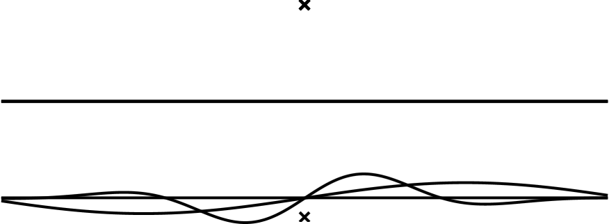
Figure 5.1: fig2

Example 2 We consider the rough surface $\Gamma_{2}$ is the flat plane $x_{2}=-1$ and the incident wave is the plane wave $u^{i}=e^{\textrm{i}kx\cdot d}$ with $d$ defined as in Section 2. Then the reference wave $u^{0}$ is defined by the formula (2.2). The total wave $u^{tol}$ is sum of the reference wave $u^{0}$ and the scattered wave $u^{s}$. Then from the discuss in the Remark 2.4, for the problem (DBVP), $u^{s}$ satisfies the Dirichlet boundary value condition $g=-u^{0}$ on $\Gamma$. For the problem (IBVP), $u^{s}$ satisfies the Impedance boundary value condition $g=-\partial u^{0}/\partial\nu+\textrm{i}k_{+}\beta u^{0}$ on $\Gamma$. Then by using Nystrom in Section 2, we can obtain the approximation of $u^{s}$.

On the other hand, the accurate total wave $u^{tol}$ can be written in the form

$$u^{0}=\begin{cases}Ae^{\textrm{i}k_{+}x\cdot d}+Be^{\textrm{i}k_{+}x\cdot d_{r}}\\ Ce^{\textrm{i}k_{-}x\cdot d_{t}}+De^{\textrm{i}k_{-}x\cdot d_{n}}\end{cases}$$ (5.10)

where $d$, $d_{r}$, $d_{t}$ are same as the Section 2 and $d_{n}=(\cos(\theta_{d}^{t}),-\sin(\theta_{d}^{t}))$ is the reflection direction of $d_{t}$.

Since $u^{tol}$ satisfies the transimssion conditon on $\Gamma_{0}$, it’s easy to solve a linear system to get the constant $A$-$D$ for specific paramater $d$. Here for the problem (IBVP), we assume $\beta\equiv 1$ on $\Gamma$.

Table 5.2 shows the value of the approximate solution of $u^{tol}$ and the exact solution evaluated by the formula (5.10). Here, we choose $\theta_{d}=\frac{4}{3}\pi$, and $x:=(1,-0.2)$.

		(DBVP)		(IBVP)
	N	Re $u^{\textrm{tol}}$	Im $u^{\textrm{tol}}$	Re $u^{\textrm{tol}}$	Im $u^{\textrm{tol}}$
$k_{+}=2.7$	8	0.798109644166213	0.326336476653307	0.643877186700853	- 0.508519378489220
$k_{-}=3.5$	16	0.806295320418223	0.329575947260149	0.643896922822836	- 0.508572132027577
	32	0.811952831200669	0.330754262490546	0.643903707281504	- 0.508608036987967
	64	0.815222519546375	0.331236659922522	0.643905536399589	- 0.508628683150847
Exact		0.737691867188743	0.215552888696214	0.643898669829883	- 0.508543039062194
$k_{+}=3.5$	8	0.346239782516876	- 2.095515135920716	0.301529983113976	- 1.297271330308942
$k_{-}=2.7$	16	0.346621218288497	- 2.095064810178228	0.301574627463057	- 1.297140425006730
	32	0.346891654083068	- 2.094828894438263	0.301608307352035	- 1.297069447803316
	64	0.347045771782107	- 2.094711378197268	0.301628429757971	- 1.297032687185948
Exact		0.347332742418633	- 2.094506667524657	0.301680817549291	- 1.296995588516340

Table 5.2: Table 2

Example 3 This example considers the periodic rough surface $\Gamma_{3}$ (see Figure 5.1 (b) ).

$$\Gamma_{3}:\quad f_{3}(t)=-1+0.16\sin(0.3\pi t);$$

The incident wave is $u^{i}=e^{\textrm{i}k_{+}x\cdot d}$ with $d$ defined as in Section 2. Like Example 2, $u^{tol}=u^{0}+u^{s}$ with $u^{0}$ defined by the formula 2.2. $u^{s}$ satisfies the Dirichlet boundary condition $g=-u^{0}$ for the problem (DBVP). $u^{s}$ satisfies the Impedance boundary condition $g=-\partial u^{0}/\partial\nu+\textrm{i}k_{-}\beta u^{0}$ on $\Gamma$ for the problem (IBVP). Here we assume $\beta\equiv 1$ on $\Gamma$. Then use the Nystrom method in Section 2 can get the approximate solution of $u^{s}$.

Table 5.3 shows the apporximate total field. The ‘exact’ solution is evaluated by using PML method (see reference [14]). Here, we choose $\theta_{d}=\frac{17}{12}\pi$, $x=(1,0.3)$.

		(DBVP)		(IBVP)
	N	Re $u^{tol}$	Im $u^{tol}$	Re $u^{tol}$	Im $u^{tol}$
$k_{+}=3$	8	-0.954594642646012	- 1.349995713793794	-0.237849526789411	- 1.015326348371200
$k_{-}=4$	16	-0.949486976255795	- 1.339216139467032	-0.237858074439157	- 1.015319402276932
	32	-0.946546398542667	- 1.333738346780402	-0.237863290074965	- 1.015315197658311
	64	-0.944852841566305	- 1.331091527595565	-0.237865914715627	- 1.015312589980869
Exact		-0.922795667915031	- 1.322211146389372	-0.247148842579830	- 1.014655415145620
$k_{+}=4$	8	-0.489478526794014	0.043905668522523	-0.434321920755574	- 0.761634578756699
$k_{-}=3$	16	-0.490441440386364	0.043990327178264	-0.434365414640936	- 0.761642059345937
	32	-0.491030962438580	0.044031752635781	-0.434392176639214	- 0.761644227331032
	64	-0.491357758704568	0.044076306711977	-0.434406993647630	- 0.761644567519472
Exact		-0.546835650859585	0.070282309134534	-0.469396042540813	- 0.732309495290609

Table 5.3: Table 3

Appendix A Potential theory

In this section, we always assume $f$ belongs to

$$B(c_{1},c_{2}):=\left\{f\in C^{1,1}(\mathbb{R}):f(s)\geq-c_{1},s\in\mathbb{R},\|f\|_{C^{1,1}(\mathbb{R})}\leq c_{2}\right\}$$

here $c_{1},c_{2}>0$.

In view of the definition and properties of the two-layered Green funciton (3.4) and (3.5), we can prove the following Theorems A.1–A.5 similarly as the reference [35, Appendix A].

Theorem A.1.

Let $W$ be the double-layer potential with density $\psi\in BC(\Gamma)$, that is

$$W(x):=\int_{\Gamma}\frac{\partial G}{\partial\nu}(x,y)\psi(y)ds(y)$$

where $\nu$ denotes the unit normal of $\Gamma$ pointing to the exterior of D. Then the following results hold.

(i) $W\in C^{2}(\mathbb{R}^{2}\backslash(\Gamma_{0}\cup\Gamma))$ and satisfies the Helmholtz equation equation and transmission boundary condition on $\Gamma_{0}$, i.e.,

$$\begin{cases}\Delta W+k_{+}^{2}W=0,\text{ in }U_{0},\\ \Delta W+k_{-}^{2}W=0,\text{ in }\mathbb{R}\backslash(\overline{U}_{0}\cap\Gamma),\\ W_{+}=W_{-},\partial_{2}W\left|{}_{+}=\partial_{2}W\right|_{-}\text{ on }\Gamma_{0}\end{cases}$$

(ii) $W$ can be continuously extended from $D$ to $\overline{D}$ and from $\mathbb{R}^{2}\backslash\overline{D}$ to $\mathbb{R}^{2}\backslash D$ with limiting values

$$W_{\pm}(x)=\int_{\Gamma}\frac{\partial G}{\partial\nu(y)}(x,y)\psi(y)ds(y)\mp\frac{1}{2}\psi(x),\quad x\in\Gamma,$$

where

$$W_{\pm}(x):=\lim_{h\to 0+}W(x\mp h\nu(x)),\quad x\in\Gamma.$$ (A.1)

The integral exists in the sense of improper integral.

(iii) $W$ satisfies

$$\sup_{\mathbb{R}^{2}\backslash\Gamma}\left|(|x_{2}|+1)^{-\frac{1}{2}}W(x)\right|<\infty.$$

(iv) There holds

$$(\nabla W(x+h\nu(x))-\nabla W(x-h\nu(x)))\cdot\nu(x)\to 0$$

as $h\to 0$, uniformly in compact subsets of $\Gamma$.

(v) $W$ satisfies UPRC (2.1) with wave number $k_{+}$ in $U_{0}$, and DPRC with wave number $k_{-}$ in $\mathbb{R}^{2}\backslash\overline{U}_{f_{-}}$, that is, there exists some $h<f_{-}$, and $\phi\in L^{\infty}(\Gamma_{h})$, such that

$$v(x)=-2\int_{\Gamma_{h}}\frac{\partial\Phi_{k_{-}}(x,y)}{\partial y_{2}}\phi(y)ds(y),x\in\mathbb{R}^{2}\backslash\overline{U}_{h}.$$

Theorem A.2.

Let $V$ be the single-layer potential with density $\psi\in BC(\Gamma)$, that is

$$V(x):=\int_{\Gamma}G(x,y)\psi(y)ds(y)$$

Then the following results hold.

(i) $V\in C^{2}(\mathbb{R}^{2}\backslash(\Gamma_{0}\cup\Gamma))$ and satisfies the Helmholtz equation equation and transmission boundary condition on $\Gamma_{0}$, i.e.,

$$\begin{cases}\Delta V+k_{+}^{2}V=0,\text{ in }U_{0},\\ \Delta V+k_{-}^{2}V=0,\text{ in }\mathbb{R}\backslash(\overline{U}_{0}\cap\Gamma),\\ V_{+}=V_{-},\partial_{2}V\left|{}_{+}=\partial_{2}V\right|_{-}\text{ on }\Gamma_{0}.\end{cases}$$

(ii) $V$ is continuous in $\mathbb{R}^{2}$, and

$$V(x) =\int_{\Gamma}G(x,y)\psi(y)ds(y),\quad x\in\Gamma,$$ (A.2)

$$\frac{\partial V_{\pm}}{\partial\nu}(x) =\int_{\Gamma}\frac{\partial G}{\partial\nu(x)}(x,y)\psi(y)ds(y)\pm\frac{1}{2}\psi(y),\quad x\in\Gamma,$$ (A.3)

where

$$\frac{\partial V_{\pm}}{\partial\nu}(x):=\lim_{h\to 0+}\nu(x)\cdot\nabla V(x\mp h\nu(x))$$ (A.4)

and this limit uniformly exists on any compact subset of $\Gamma$, and the integrals in (A.2) and (A.3) exist as improper integrals.

(iii) $V$ satisfies

$$\sup_{\mathbb{R}^{2}\backslash\Gamma}\left|(|x_{2}|+1)^{-\frac{1}{2}}v(x)\right|<\infty.$$

(iv) $V$ satisfies UPRC (2.1) with wave number $k_{+}$ in $U_{0}$, and DPRC with wave number $k_{-}$ in $\mathbb{R}^{2}\backslash\overline{U}_{f_{-}}$, that is, there exists some $h<f_{-}$, and $\phi\in L^{\infty}(\Gamma_{h})$, such that

$$v(x)=-2\int_{\Gamma_{h}}\frac{\partial\Phi_{k_{-}}(x,y)}{\partial y_{2}}\phi(y)ds(y),x\in\mathbb{R}^{2}\backslash\overline{U}_{h}.$$

Theorem A.3.

Let $\psi\in BC(\Gamma)$, then the direct values of the single-layer potential

$$V(x):=\int_{\Gamma}\frac{\partial G}{\partial\nu(y)}(x,y)\psi(y)ds(y),\quad x\in\Gamma$$

and the single-layer potential

$$V(x):=\int_{\Gamma}G(x,y)\psi(y)ds(y),\quad x\in\Gamma$$

represent uniformly Hölder functions on $\Gamma$ with

$$\|V\|_{C^{0,\lambda}},\|W\|_{C^{0,\lambda}}\leq C\|\psi\|_{\infty,\Gamma},$$

for $\psi\in BC(\Gamma)$.

Theorem A.4.

Let $\psi\in C^{0,1}(\Gamma)$ with $0<\lambda<1$, then

$$|\nabla W(X)|\leq C|f(x_{1})-x_{2}|^{\lambda-1},\quad x\in U_{b_{1}}\backslash(\overline{U}_{b_{2}}\cup\Gamma)$$

where $C$ is a positive constant and $b_{1}=-f_{-}-1$, $b_{2}=f_{+}/2$.

Theorem A.5.

Let $\psi\in BC(\Gamma)$, then for $0<\lambda<1$, there exists a positive constant $C$ such that

$$|\nabla V(x)|\leq C|f(x_{1})-x_{2}|^{\lambda-1},\quad x\in U_{b_{1}}\backslash(\overline{U}_{b_{2}}\cup\Gamma)$$

where $C$ is a positive constant and $b_{1}=f_{-}-1$, $b_{2}=f_{+}/2$.

Appendix B Integral operators on the real line

Define the integral equation operator $\mathscr{K}_{l}$ with kernel $l:\mathbb{R}^{2}\to\mathbb{C}$ by

$$\mathscr{K}_{l}\psi(s):=\int_{\mathbb{R}}l(s,t)\psi(t)dt,\quad s\in\mathbb{R}$$ (B.1)

It is seen that the integral (B.1) exists in a Lebesgue sense for every $\psi\in X:=L^{\infty}(\mathbb{R})$ and $s\in\mathbb{R}$ iff $l(s,\cdot)\in L^{1}(\mathbb{R}),s\in\mathbb{R}$. $\mathscr{K}_{l}:X\to Y:=BC(\mathbb{R})$ and is bounded iff $l(s,\cdot)\in L^{1}(\mathbb{R}),s\in\mathbb{R}$ and

$$|\|l\||:=\textrm{ess}\sup_{s\in\mathbb{R}}\|l(s,\cdot)\|_{1}<\infty$$ (B.2)

and $\mathscr{K}_{l}\psi\in C(\mathbb{R})$ for every $\psi\in X$.

In the case that (B.2) holds, we identity $l:\mathbb{R}^{2}\to\mathbb{C}$ with the mapping $s\to l(s,\cdot)$ in $Z:=L^{\infty}(\mathbb{R},L^{1}(\mathbb{R}))$, which mapping is essentially bounded with norm $|\|l\||$. Let $K$ denote the set of those functions $l\in Z$ having the property that $\mathscr{K}_{l}\psi\in C(\mathbb{R})$ for every $\psi\in X$, where $\mathscr{K}_{l}$ is the integral operator (B.1). $Z$ is a Banach space with the norm $|\|\cdot\||$ and $K$ is a closed subspace of $Z$. $\mathscr{K}_{l}:X\to Y$ and is bounded iff $l\in K$. Let $BC(\mathbb{R},L^{1}(\mathbb{R}))$ denote the set of those functions $l\in Z$ having the property that for all $s\in\mathbb{R}$,

$$\|l(s,\cdot)-l(s^{\prime},\cdot)\|\to 0,\textrm{ as }s^{\prime}\to s.$$

Then it is easy to be seen that that $BC(\mathbb{R},L^{1}(\mathbb{R}))\subset K$.

For $\phi_{n}\subset Y$ and $\phi\in Y$, we say that $(\phi_{n})$ converges strictly to $\phi$ and write $\phi_{n}\stackrel{{\scriptstyle s}}{{\rightarrow}}\phi$ if $\sup_{n\in\mathbf{N}}$ $\left\|\phi_{n}\right\|_{\infty}<\infty$ and $\phi_{n}(t)\rightarrow\phi(t)$ uniformly on every compact subset of $\mathbb{R}$. For $l_{n}\subset K$, $l\in K$, we say that $(l_{n})$ is $\sigma$-convergence to $l$ and write $l_{n}\stackrel{{\scriptstyle\sigma}}{{\to}}$ if $\sup_{n\in\mathbb{N}}|\|l_{n}\||<\infty$ and for all $\psi\in X$,

$$\int_{\mathbb{R}}l_{n}(s,t)\psi(t)dt\to\int_{\mathbb{R}}l(s,t)\psi(t)dt$$

as $n\to\infty$, unifromly on every compact subset of $\mathbb{R}$.

For $a\in\mathbb{R}$, define the translation operator $T:\textbf{Z}\to\textbf{Z}$ by

$$T_{a}l(s,t)=l(s-a,t-a),\quad s,t\in\mathbb{R}$$

We say that a subset $W\subset K$ is $\sigma$-sequentially compact in $K$ if each sequence in $W$ has a $\sigma$-convergent subsequence with limit in $W$. Let $B(Y)$ denote the bounded the Banach space of bounded linear operators on $Y$. Let $I$ denote the identity operator on $Y$.

The following result on the invertibility of $I-\mathscr{K}_{l}$ is proved in the reference [12].

Lemma B.1.

Suppose that $W\subset\mathbf{K}$ is $\sigma$-sequentially compact and satisfies that, for all $s\in\mathbb{R}$,

$$\sup_{l\in W}\int_{\mathbb{R}}\left|l(s,t)-l\left(s^{\prime},t\right)\right|\mathrm{d}t\rightarrow 0,\quad\text{ as }s^{\prime}\rightarrow s$$ (B.3)

that $T_{a}(W)=W$ for some $a\in\mathbb{R}$, and that $I-\mathscr{K}_{l}$ is injective for all $l\in W$. Then $\left(I-\mathscr{K}_{l}\right)^{-1}$ exists as an operator on the range space $\left(I-\mathscr{K}_{l}\right)(Y)$ for all $l\in W$ and

$$\sup_{l\in W}\left\|\left(I-\mathscr{K}_{l}\right)^{-1}\right\|<\infty$$

If also, for every $l\in W$, there exists a sequence $\left(l_{n}\right)\subset W$ such that $l_{n}\stackrel{{\scriptstyle\sigma}}{{\rightarrow}}l$ and, for each $n$, it holds that

$$I-\mathscr{K}_{l_{n}}\text{ injective }\Rightarrow I-\mathscr{K}_{l_{n}}\text{ surjective }$$ (B.4)

then also $I-\mathscr{K}_{l}$ is surjective for each $l\in W$ so that $\left(I-\mathscr{K}_{l}\right)^{-1}\in B(Y)$.

With the help of the properties of the two-layered Green function $G(x,y)=G_{D}(x,y)+G_{R}(x,y)$ for $x_{2},y_{2}<0$ and the estimate (3.4). The following Lemmas B.2, B.4 and B.5 can be proved similarly as the reference [35, Lemma B.2, B.3, B.4].

Lemma B.2.

Let $\kappa\in L^{1}(\mathbb{R})$ be defined by

$$\kappa(s):=\begin{cases}1-\textrm{log}|s|,\quad 0<|s|\leq 1,\\ |s|^{-3/2},\quad|s|>1.\end{cases}$$

(i) For all $f\in B$,

$$\left|\kappa_{f}(s,t)\right|\leq C\left|\kappa(s-t)\right|,\quad s,t\in\mathbb{R},\;s\neq t$$

for some constant $C>0$ depending only on $c_{1}$, $c_{2}$, $\eta$, and $\kappa$, and

$$\sup_{|s_{1}-s_{2}|\leq h,f\in B}\int_{\mathbb{R}}\left|k_{f}(s_{1},t)-\kappa_{f}(s_{2},t)\right|dt\to 0$$

as $h\to 0$.

(ii) For all $f\in B,\tilde{\beta}\in E$, there holds

$$\left|\kappa_{\tilde{\beta},f}(s,t)\right|\leqslant C\left|\kappa(s-t)\right|,\quad s,t\in\mathbb{R},\quad s\neq t$$

for some constant $C>0$ depending only on $c_{1},c_{2},d_{2}$, and $\kappa$, and

$$\sup_{\left|s_{1}-s_{2}\right|\leqslant h,f\in B,\tilde{\beta}\in E}\int_{\mathbb{R}}\left|\kappa_{\tilde{\beta},f}\left(s_{1},t\right)-\kappa_{\tilde{\beta},f}\left(s_{2},t\right)\right|\mathrm{d}t\rightarrow 0$$

as $h\rightarrow 0$.

Definition B.3.

$$B =B\left(c_{1},c_{2}\right):=\left\{f\in C^{1,1}(\mathbb{R}):f(s)\geqslant c_{1},s\in\mathbb{R}\text{ and }\|f\|_{C^{1,1}(\mathbb{R})}\leqslant c_{2}\right\}$$

$$E =E\left(d_{1},d_{2},\omega\right):=\left\{\tilde{\beta}\in Y:\Re(\tilde{\beta}(s))\geqslant d_{1},s\in\mathbb{R},\|\tilde{\beta}\|_{\infty}\leqslant d_{2},\right.\text{ and }|\tilde{\beta}(s)-\tilde{\beta}(t)|\leqslant\omega(|s-t|),s,t\in\mathbb{R}\}$$

Lemma B.4.

(i) Every sequence $\left(f_{n}\right)\subset B$ has a subsequence $\left(f_{n_{m}}\right)$ such that $f_{n_{m}}\stackrel{{\scriptstyle s}}{{\rightarrow}}f$, $f_{n_{m}}^{\prime}\stackrel{{\scriptstyle s}}{{\rightarrow}}f^{\prime}$, with $f\in B$.

(ii) Suppose that $\left(f_{n}\right)\subset B$ and that $f_{n}\stackrel{{\scriptstyle s}}{{\rightarrow}}f$, $f_{n}^{\prime}\stackrel{{\scriptstyle s}}{{\rightarrow}}f^{\prime}$, with $f\in B$. Then $\kappa_{f_{n}}\stackrel{{\scriptstyle\sigma}}{{\rightarrow}}\kappa_{f}$.

Lemma B.5.

(i) Every sequence $\left(\tilde{\beta}_{n}\right)\subset E$ has a subsequence $\left(\tilde{\beta}_{n_{m}}\right)$ such that $\tilde{\beta}_{n_{m}}\stackrel{{\scriptstyle s}}{{\rightarrow}}\tilde{\beta}$ with $\tilde{\beta}\in E$.

(ii) If $\left(f_{n}\right)\subset B$, $\left(\tilde{\beta}_{n}\right)\subset E$ and $f_{n}\stackrel{{\scriptstyle s}}{{\rightarrow}}f$, $f_{n}^{\prime}\stackrel{{\scriptstyle s}}{{\rightarrow}}f^{\prime}$, $\tilde{\beta}_{n_{m}}\stackrel{{\scriptstyle s}}{{\rightarrow}}\tilde{\beta}$, with $f\in B$ and $\tilde{\beta}\in E$, then $\kappa_{\tilde{\beta_{n}},f_{n}}\stackrel{{\scriptstyle\sigma}}{{\rightarrow}}\kappa_{\tilde{\beta},f}$.

References

• [1] M. Abramowitz and I. A. Stegun, Handbook of mathematical functions with formulas, graphs, and mathematical tables, National Bureau of Standards Applied Mathematics Series, No. 55, Washington, D.C., 1964.
• [2] K. E. Atkinson, The Numerical Solution of Integral Equations of the Second Kind, Cambridge University Press, 1997.
• [3] S. N. Chandler-Wilde and J. Elschner, Variational approach in weighted sobolev spaces to scattering by unbounded rough surfaces, SIAM J. Math. Anal., 42 (2010), 2554–2580.
• [4] S. N. Chandler-Wilde and P. Monk, Existence, uniqueness, and variational methods for scattering by unbounded rough surfaces, SIAM J. Math. Anal., 37 (2005), 598–618.
• [5] S. N. Chandler-Wilde and P. Monk, The pml for rough surface scattering, Appl. Numer. Math., 59 (2009), 2131–2154.
• [6] S. N. Chandler-Wilde, C. R. Ross and B. Zhang, Scattering by infinite one-dimensional rough surfaces, R. Soc. Lond. Proc., A 455 (1999), 3767–3787.
• [7] S. N. Chandler-Wilde and C. R. Ross, Scattering by rough surfaces: the Dirichlet problem for the Helmholtz equation in a non-locally perturbed half-plane, Math. Methods Appl. Sci., 19 (1996), 959–976.
• [8] S. N. Chandler-Wilde and B. Zhang, On the solvability of a class of second kind integral equations on unbounded domains, J. Math. Anal. Appl., 214 (1997), 482–502.
• [9] S. N. Chandler-Wilde and B. Zhang, Electromagnetic scattering by an inhomogeneous conducting or dielectric layer on a perfectly conducting plate, R. Soc. Lond. Proc., A 454 (1998), 519–542.
• [10] S. N. Chandler-Wilde and B. Zhang, A uniqueness result for scattering by infinite rough surfaces, SIAM J. Appl. Math., 58 (1998), 1774–1790.
• [11] S. N. Chandler-Wilde and B. Zhang, Scattering of electromagnetic waves by rough interfaces and inhomogeneous layers, SIAM J. Math. Anal., 30 (1999), 559–583.
• [12] S. N. Chandler-Wilde, B. Zhang and C. R. Ross, On the solvability of second kind integral equations on the real line, J. Math. Anal. Appl., 245 (2000), 28–51.
• [13] S. Chandler-Wilde, Boundary value problems for the helmholtz equation in a half-plane, in Third International Conference on Mathematical and Numerical Aspects of Wave Propagation, vol. 77, SIAM, 1995, 188.
• [14] Z. Chen and H. Wu, An adaptive finite element method with perfectly matched absorbing layers for the wave scattering by periodic structures, SIAM J. Numer. Anal., 41 (2003), 799–826.
• [15] W. C. Chew, Waves and fields in inhomogenous media, vol. 16, John Wiley & Sons, 1999.
• [16] D. Colton and R. Kress, Inverse acoustic and electromagnetic scattering theory, 4th edition, Applied Mathematical Sciences, Springer, New York, 2019.
• [17] J. DeSanto, Scattering by rough surfaces, in Scattering, Elsevier, 2002, 15–36.
• [18] J. Elschner and G. Hu, Elastic scattering by unbounded rough surfaces, SIAM J. Math. Anal., 44 (2012), 4101–4127.
• [19] J. Elschner and G. Hu, Elastic scattering by unbounded rough surfaces: solvability in weighted sobolev spaces, Appl. Anal., 94 (2015), 251–278.
• [20] D. Gilbarg and N. S. Trudinger, Elliptic partial differential equations of second order, 2nd edition, Springer, Berlin, 1983.
• [21] H. Haddar and A. Lechleiter, Electromagnetic wave scattering from rough penetrable layers, SIAM J. Math. Anal., 43 (2011), 2418–2443.
• [22] G. Hu, P. Li and Y. Zhao, Elastic scattering from rough surfaces in three dimensions, J. Differential Equations, 269 (2020), 4045–4078.
• [23] G. Hu, X. Liu, F. Qu and B. Zhang, Variational approach to scattering by unbounded rough surfaces with Neumann and generalized impedance boundary conditions, Commun. Math. Sci., 13 (2015), 511–537.
• [24] A. Kirsch and A. Lechleiter, The limiting absorption principle and a radiation condition for the scattering by a periodic layer, SIAM J. Math. Anal., 50 (2018), 2536–2565.
• [25] L. Li, J. Yang, B. Zhang and H. Zhang, Uniform far-field asymptotics of the two-layered green function in 2d and application to wave scattering in a two-layered medium, arXiv preprint arXiv:2208.00456.
• [26] P. Li, H. Wu and W. Zheng, Electromagnetic scattering by unbounded rough surfaces, SIAM J. Math. Anal., 43 (2011), 1205–1231.
• [27] A. Meier, T. Arens, S. N. Chandler-Wilde and A. Kirsch, A Nyström method for a class of integral equations on the real line with applications to scattering by diffraction gratings and rough surfaces, J. Integral Equations Appl., 12 (2000), 281–321.
• [28] C. A. Pérez Arancibia, Windowed integral equation methods for problems of scattering by defects and obstacles in layered media, PhD thesis, California Institute of Technology, 2017.
• [29] R. Petit (ed.), Electromagnetic theory of grating, Springer, 1980.
• [30] M. Saillard and A. Sentenac, Rigorous solutions for electromagnetic scattering from rough surfaces, Waves in random media, 11 (2001), 103–137.
• [31] E. M. Stein and R. Shakarchi, Princeton lectures in analysis, Princeton University Press Princeton, 2003.
• [32] A. G. Voronovich, Wave scattering from rough surfaces, Springer, New York, 1999.
• [33] K. F. Warnick and W. C. Chew, Numerical simulation methods for rough surface scattering, Waves in Random Media, 11 (2001), R1–R30.
• [34] B. Zhang and S. N. Chandler-Wilde, Acoustic scattering by an inhomogeneous layer on a rigid plate, SIAM J. Appl. Math., 58 (1998), 1931–1950.
• [35] B. Zhang and S. N. Chandler-Wilde, Integral equation methods for scattering by infinite rough surfaces, Math. Methods Appl. Sci., 26 (2003), 463–488.
• [36] B. Zhang and R. Zhang, An FFT-based algorithm for efficient computation of Green’s functions for the Helmholtz and Maxwell’s equations in periodic domains, SIAM J. Sci. Comput., 40 (2018), B915–B941.
• [37] R. Zhang, High order complex contour discretization methods to simulate scattering problems in locally perturbed periodic waveguides, SIAM J. Sci. Comput., 44 (2022), B1257–B1281.